---
execute:
echo: true
eval: true
bibliography: ["../references.bib", "../refs/ch-33.bib"]
---
# Future Directions and Open Problems {#sec-ch33}
::: {.callout-note appearance="simple" icon="false"}
**Scope: both retail and corporate.** Open problems and forward-looking themes (synthetic data, federated learning, climate risk, agentic underwriting) cut across portfolios.
:::
## Overview {.unnumbered}
Every chapter in this book has pushed a specific method, a specific dataset, and a specific regulatory context. This final chapter looks outward. It takes the body of credit scoring research as it stands at the start of 2026 and asks what the next decade of practice should look like. The answer is not a single new model. It is a reshuffling of where data lives, how models are trained across institutional boundaries, how scoring systems ingest information in real time, how regulators expect to audit those systems, and where empirical credit work still has unsolved foundational problems.
The chapter is organized around seven themes. Federated learning (@sec-ch33) addresses the fact that credit data is partitioned across banks, credit bureaus, telcos, and e-commerce platforms, and that pooling raw data is often legally impossible. Synthetic data (@sec-ch33-synthetic) answers the near identical question from the opposite direction: when data cannot move, can we move a statistical imitation of it? Streaming scoring (@sec-ch33-streaming) tackles the engineering shift from nightly batch decisioning to sub-second decisioning. Multimodal models (@sec-ch33-multimodal) wire together the tabular scorecards, the text underwriting notes, the graph of guarantors, and the satellite images of collateral that modern credit teams already possess in isolation. Quantum ML (@sec-ch33-quantum) is the section where most of the marketing ends and most of the engineering begins. Regulation (@sec-ch33-reg) walks through the EU AI Act timeline, the CFPB circulars, and the ECB supervisory expectations that turn these methods from optional research directions into compliance constraints. The final section (@sec-ch33-open) closes with ten concrete research problems that have been referenced throughout the book but never solved.
A working theme runs through all of this. Credit scoring is a field whose constraints are increasingly set not by modeling capacity but by data governance. The capacity to fit a 100M-parameter transformer on payment transcripts exists today on a single GPU node; the legal right to pool those transcripts across institutions does not. The frontier of the field is therefore the frontier of mechanisms, cryptographic, statistical, architectural, that let a model see more than any single institution can lawfully share.
Emerging markets push this frontier harder than mature ones. Thin bureau coverage, rapid mobile adoption, fragmented data holders, and activist regulators produce conditions where federated learning, synthetic data, and alternative signals are not research aspirations but near-term operational requirements [@bjorkegren2020behavior; @adb_vietnam_fintech2022]. Vietnam is a useful reference case: the State Bank issued a formal fintech sandbox decree in 2025, a digital transformation roadmap to 2030, and a CBDC research mandate, all while MSME credit gaps remain wide [@sbv_decree94_2025; @sbv_digital_roadmap2021; @worldbank2022vietnamfinance].
### Notation {.unnumbered}
- $K$ indexes banks or data holders in a federation, $K \in \{1, 2, \dots, M\}$.
- $\mathcal{D}_k = \{(x_i^{(k)}, y_i^{(k)})\}_{i=1}^{n_k}$ is the local dataset at party $k$.
- $w \in \mathbb{R}^p$ denotes model parameters shared across parties.
- $F_k(w)$ is the local empirical risk at party $k$; $F(w) = \sum_k (n_k/n) F_k(w)$ the global objective.
- $(\varepsilon, \delta)$ are the parameters of a differentially private mechanism.
- $\Delta_2 f$ is the $\ell_2$ sensitivity of a function $f$.
- $\mathcal{N}(\mu, \sigma^2)$ is the Gaussian distribution.
- $T$ denotes the number of FedAvg rounds; $E$ the number of local epochs per round.
- $q$ denotes queries-per-second to a production scoring endpoint.
- $\tau$ end-to-end scoring latency (ms); $\tau_\text{feat}, \tau_\text{infer}, \tau_\text{post}$ its components.
```{python}
#| echo: true
#| output: false
import sys, os, time, json, math, warnings
sys.path.insert(0, "../code")
import numpy as np
import pandas as pd
import matplotlib.pyplot as plt
from sklearn.linear_model import LogisticRegression
from sklearn.preprocessing import StandardScaler
from sklearn.metrics import roc_auc_score, brier_score_loss
from sklearn.model_selection import train_test_split
warnings.filterwarnings("ignore")
np.random.seed(7)
from creditutils import load_german_credit, gini, ks_statistic, stable_sigmoid
```
## Federated learning in credit {#sec-ch33-future}
Credit data never sits in one place. A prime-card issuer sees spending patterns but not mortgages; a mortgage originator sees loan-to-value and payment history but not revolving utilization; a telco sees prepaid top-ups that predict default among thin-file borrowers [@bjorkegren2020behavior] but has no loan performance data at all. In principle, pooling these sources would yield a richer feature space and better calibration. In practice, data protection law, competitive dynamics, and cost sharing disputes make pooling difficult or illegal. Federated learning (FL) is the response. A model is trained across the parties without the raw data ever leaving the institution that holds it [@mcmahan2017communication; @kairouz2021advances; @yang2019federated].
There are two dominant architectures. Horizontal FL (HFL) partitions the sample space: bank $A$ and bank $B$ hold different customers with the same features. This is the setting McMahan et al. originally studied for on-device learning across millions of phones [@mcmahan2017communication]; it also fits a consortium of regional banks fitting a common default model. Vertical FL (VFL) partitions the feature space: the same customers are held by bank $A$ and telco $B$, and the challenge is to train a joint model on $x^A \oplus x^B$ without either party revealing $x^A$ or $x^B$ to the other [@hardy2017private; @cheng2021secureboost].
### Motivating use cases
Three practical settings recur in consumer and SME credit.
Multi-bank consortium for fraud and thin-file scoring. Small regional banks individually lack enough default events to estimate a reliable low-default-portfolio model. A consortium of ten regional banks can federate a shared model on aligned features without pooling customer-level records. Each bank gets a richer model than it could fit alone; no bank exposes its book. This has appeared in early production at European mutuals and U.S. community bank consortia.
Bank plus non-bank alternative data. A bank has loan performance labels; a telco or e-commerce platform holds behavioral features that predict default in segments the bureau does not cover [@berg2020rise]. Neither party can legally hand over raw data. Vertical FL with secure intersection gives the bank access to the predictive content of those features on the intersecting customer base.
Credit bureau augmentation. Instead of a bureau aggregating the tradelines of every customer at every participating bank, the bureau hosts the training orchestration and global parameters; local tradelines never leave the originating bank. Bureau output remains a public score but the training pipeline becomes privacy-first.
In each case the question is whether the statistical gain from federation exceeds the cost in engineering, latency, and residual privacy risk.
### FedAvg and its convergence
The canonical horizontal FL algorithm is FedAvg [@mcmahan2017communication]. In round $t$, the server broadcasts the current global model $w^{(t)}$. Each party $k$ runs $E$ epochs of local SGD on $\mathcal{D}_k$, returning its updated parameters $w_k^{(t+1)}$. The server aggregates:
$$
w^{(t+1)} = \sum_{k=1}^{M} \frac{n_k}{n} w_k^{(t+1)}.
$$ {#eq-fedavg-update}
Here $n_k = |\mathcal{D}_k|$ and $n = \sum_k n_k$. With $E = 1$ and full participation, FedAvg reduces to synchronous mini-batch SGD on the union of the datasets and inherits its convergence. With $E > 1$, parties drift between aggregation steps; the convergence bound degrades. Under $L$-smoothness of each $F_k$ and bounded gradient dissimilarity
$$
\frac{1}{M}\sum_k \lVert \nabla F_k(w) - \nabla F(w) \rVert^2 \le \sigma^2,
$$
Li et al. [@li2020federated] give the asymptotic bound
$$
\mathbb{E}\bigl[ F(\bar w^{(T)}) - F(w^\star) \bigr] \le \mathcal{O}\!\left(\frac{1}{\eta T}\right) + \mathcal{O}(\eta E \sigma^2),
$$ {#eq-fedavg-conv}
where $\eta$ is the local learning rate and $\bar w^{(T)}$ the running average. Two terms trade off. Increasing $E$ reduces communication rounds but inflates the drift term $\eta E \sigma^2$. When the parties are statistically heterogeneous ($\sigma^2$ large, think: one bank is retail, one is SME, one is mortgage) FedAvg either needs more rounds or a smaller $\eta$. This heterogeneity gap is the single largest reason naive FedAvg underperforms centralized training in real credit deployments.
For a convex loss, a tighter bound holds. With step size $\eta_t = 1/(\mu(t+\gamma))$ for $\mu$-strongly-convex $F$ and bounded variance, @li2020federated prove
$$
\mathbb{E}[F(w^{(T)})] - F(w^\star) \le \frac{\kappa}{\gamma + T}\left( B + C E \right),
$$ {#eq-fedavg-strong}
where $\kappa = L/\mu$ is the condition number, $B$ aggregates the initial distance to optimum and stochastic variance, and $C$ the heterogeneity. Increasing $E$ hurts; increasing heterogeneity hurts; making the loss better conditioned helps. These insights should inform a credit FL deployment: standardize features across parties, choose losses with good conditioning (regularized logistic over pure ERM), and pick $E$ per the empirical gradient dissimilarity.
### Differential privacy in the federation
Sending raw gradients reveals information. Gradient inversion attacks can reconstruct training examples from a single gradient update [@fredrikson2015model; @shokri2017membership]. Differential privacy (DP) [@dwork2006calibrating; @dwork2014algorithmic] provides a principled guarantee. A randomized mechanism $\mathcal{M}$ is $(\varepsilon, \delta)$-DP if for any two neighboring datasets $D, D'$ (differing by one record) and any measurable set $S$,
$$
\Pr[\mathcal{M}(D) \in S] \le e^\varepsilon \Pr[\mathcal{M}(D') \in S] + \delta.
$$ {#eq-dp-def}
For a query $f: \mathcal{D} \to \mathbb{R}^p$ with $\ell_2$-sensitivity $\Delta_2 f = \sup_{D \sim D'} \lVert f(D) - f(D') \rVert_2$, the Gaussian mechanism adds noise $\mathcal{N}(0, \sigma^2 I)$ with
$$
\sigma = \frac{\Delta_2 f \cdot \sqrt{2 \ln(1.25/\delta)}}{\varepsilon}.
$$ {#eq-gauss-dp}
DP-SGD [@abadi2016deep] applies this to gradients. At each step: clip per-example gradient norms to $C$ (giving sensitivity $C$), add Gaussian noise $\mathcal{N}(0, \sigma^2 C^2 I)$, and update. The privacy cost composes across training steps. Rényi differential privacy [@mironov2017renyi] gives tight composition: for the Gaussian mechanism with noise multiplier $\sigma$ (noise std / clip norm), the Rényi DP at order $\alpha$ is $\alpha / (2\sigma^2)$, convertible to $(\varepsilon, \delta)$-DP via
$$
\varepsilon = \inf_\alpha \left\{ \alpha / (2\sigma^2) \cdot T + \tfrac{\log(1/\delta)}{\alpha - 1} \right\}.
$$ {#eq-rdp-to-dp}
The practical takeaway: a consortium that runs DP-FedAvg at $(\varepsilon, \delta) = (3, 10^{-5})$ typically loses 2 to 5 AUC points relative to non-private centralized training; at $\varepsilon = 1$, the loss can exceed 10 points on German-Credit-scale data. Large federations with $n > 10^6$ absorb the privacy cost more easily because sensitivity scales as $C/n$.
Secure aggregation [@bonawitz2017practical] is complementary. Parties secret-share their updates such that the server sees only the sum, not individual contributions. DP protects against a curious server; secure aggregation protects against a server that honestly aggregates but would otherwise learn per-party updates. Production deployments use both.
### FedAvg toy: three simulated banks on German Credit
The goal here is pedagogical. We split the UCI German Credit dataset [@lessmann2015benchmarking] across three simulated banks with heterogeneous class mixtures, train a logistic model locally for each, and show FedAvg converging to something close to the centralized optimum. This is the smallest live example that actually reveals the FedAvg dynamics.
```{python}
#| label: prep-german
df = load_german_credit()
y = df["default"].astype(int).values
X = pd.get_dummies(df.drop(columns=["default"]), drop_first=True).astype(float).values

scaler = StandardScaler().fit(X)
X = scaler.transform(X)
X = np.hstack([X, np.ones((X.shape[0], 1))])  # intercept
p = X.shape[1]
print(f"n={X.shape[0]}, p={p}, default rate={y.mean():.3f}")

# heterogeneous partition: bank A defaults-heavy, B normal, C defaults-light
rng = np.random.default_rng(11)
perm = rng.permutation(len(y))
# stratify unevenly
idx_pos = np.where(y == 1)[0]; idx_neg = np.where(y == 0)[0]
rng.shuffle(idx_pos); rng.shuffle(idx_neg)
banks = {
    "A": np.concatenate([idx_pos[:180], idx_neg[:120]]),   # 60% default
    "B": np.concatenate([idx_pos[180:260], idx_neg[120:380]]),  # ~23% default
    "C": np.concatenate([idx_pos[260:],   idx_neg[380:]]),  # ~6% default
}
for k, idx in banks.items():
    print(f"bank {k}: n={len(idx)}, default={y[idx].mean():.3f}")
```
The three banks have class mixtures (60%, 23%, 6%) so FedAvg must reconcile quite different local optima. We fit centralized logistic regression as the reference, then simulate FedAvg with plain per-bank SGD.
```{python}
#| label: fedavg-toy
def sigmoid(z): return stable_sigmoid(np.clip(z, -35, 35))

def nll_grad(w, X, y, lam=1e-3):
    p_hat = sigmoid(X @ w)
    g = X.T @ (p_hat - y) / len(y) + lam * w
    return g

def local_update(w, X, y, lr=0.05, epochs=1, batch=64, seed=0):
    rng = np.random.default_rng(seed)
    w = w.copy()
    n = len(y)
    for _ in range(epochs):
        idx = rng.permutation(n)
        for s in range(0, n, batch):
            b = idx[s:s+batch]
            g = nll_grad(w, X[b], y[b])
            w -= lr * g
    return w

# centralized baseline
w_cen = np.zeros(p)
for _ in range(200):
    w_cen -= 0.1 * nll_grad(w_cen, X, y)

# FedAvg
rounds = 60
E_local = 2
w_fed = np.zeros(p)
history = {"round": [], "auc": [], "ll": [], "dist": []}
for t in range(rounds):
    w_locals = []
    for k, (name, idx) in enumerate(banks.items()):
        w_k = local_update(w_fed, X[idx], y[idx], lr=0.08, epochs=E_local,
                            batch=32, seed=t * 7 + k)
        w_locals.append((len(idx), w_k))
    total = sum(n_k for n_k, _ in w_locals)
    w_fed = sum((n_k / total) * wk for n_k, wk in w_locals)
    p_hat = sigmoid(X @ w_fed)
    auc = roc_auc_score(y, p_hat)
    ll = -(y * np.log(p_hat + 1e-12) + (1 - y) * np.log(1 - p_hat + 1e-12)).mean()
    history["round"].append(t); history["auc"].append(auc)
    history["ll"].append(ll)
    history["dist"].append(np.linalg.norm(w_fed - w_cen))

p_cen = sigmoid(X @ w_cen)
print(f"centralized AUC = {roc_auc_score(y, p_cen):.4f}")
print(f"FedAvg final AUC = {history['auc'][-1]:.4f}")
print(f"||w_fed - w_cen|| / ||w_cen|| = {history['dist'][-1] / np.linalg.norm(w_cen):.3f}")
```
```{python}
#| label: fig-fedavg
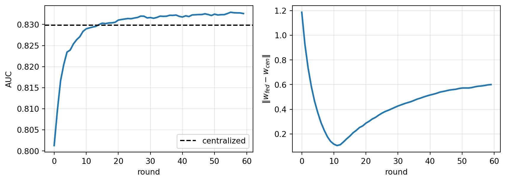
#| fig-cap: "FedAvg convergence on a three-bank simulated federation of UCI German Credit. Local epochs E=2, rounds T=60, lr=0.08."
fig, ax = plt.subplots(1, 2, figsize=(9, 3.3))
ax[0].plot(history["round"], history["auc"], lw=2)
ax[0].axhline(roc_auc_score(y, p_cen), ls="--", c="k", label="centralized")
ax[0].set_xlabel("round"); ax[0].set_ylabel("AUC"); ax[0].legend(); ax[0].grid(alpha=0.3)
ax[1].plot(history["round"], history["dist"], lw=2)
ax[1].set_xlabel("round"); ax[1].set_ylabel(r"$\|w_{fed} - w_{cen}\|$")
ax[1].grid(alpha=0.3)
fig.tight_layout(); plt.show()
```
As shown in @fig-fedavg, three lessons emerge. First, FedAvg closes most of the gap to centralized performance inside twenty rounds. Second, the parameter distance to the centralized solution does not go to zero with heterogeneous partitions; FedAvg finds a different stationary point. Third, a single round of local SGD is not enough; there is a sweet spot for $E$ that depends on how different the banks look from one another. In production, that sweet spot is tuned on held-out validation, and FedAvg is usually replaced by FedProx (which penalizes local drift) or SCAFFOLD (which corrects it with control variates).
### DP-FedAvg: privacy budget walkthrough
The next block layers Gaussian noise on the averaged update and tracks the total $\varepsilon$. We use the simple Rényi-DP composition from @mironov2017renyi.
```{python}
#| label: dp-fedavg
def rdp_gaussian(sigma_mult, steps, alpha):
    """RDP of the Gaussian mechanism at order alpha, applied `steps` times."""
    return steps * alpha / (2.0 * sigma_mult ** 2)

def rdp_to_epsilon(rdp_fn, steps, delta=1e-5, alphas=None):
    if alphas is None:
        alphas = np.arange(2, 65)
    return min(rdp_fn(s=steps, a=a) + math.log(1.0 / delta) / (a - 1)
               for a in alphas)

rng = np.random.default_rng(0)
clip_C = 1.0
sigma_mult = 1.2  # noise multiplier relative to clip
w_dp = np.zeros(p)
aucs = []
for t in range(rounds):
    deltas = []
    for name, idx in banks.items():
        w_k = local_update(w_dp, X[idx], y[idx], lr=0.08, epochs=E_local,
                            batch=32, seed=t * 13)
        d = w_k - w_dp
        # per-party clip (approximates per-sample clip at the party level)
        nrm = np.linalg.norm(d)
        d = d * min(1.0, clip_C / (nrm + 1e-12))
        deltas.append((len(idx), d))
    total = sum(n for n, _ in deltas)
    agg = sum((n / total) * d for n, d in deltas)
    # Gaussian noise scaled to clip norm
    noise = rng.normal(0, sigma_mult * clip_C / total, size=p)
    w_dp = w_dp + agg + noise
    aucs.append(roc_auc_score(y, sigmoid(X @ w_dp)))

def rdp_fn(s, a): return rdp_gaussian(sigma_mult, s, a)
eps_total = rdp_to_epsilon(rdp_fn, steps=rounds, delta=1e-5)
print(f"DP-FedAvg final AUC = {aucs[-1]:.4f}")
print(f"(epsilon, delta) after {rounds} rounds = ({eps_total:.2f}, 1e-5)")
```
The printout reports a concrete privacy budget. At $\varepsilon$ around 3 to 8 (common in academic DP-ML papers), FedAvg on this tiny dataset loses several AUC points; at $\varepsilon$ above 15 the loss becomes negligible but the guarantee is largely rhetorical. Realistic consumer-credit consortia ($n \ge 10^7$) can typically run at $\varepsilon$ in $[1, 5]$ with acceptable accuracy because the per-example sensitivity is far smaller in relative terms.
### Vertical FL for credit: sketch and caveats
Vertical FL is much harder than horizontal. The classic recipe:
1. Privacy-preserving record linkage (PPRL). The parties compute an encrypted intersection of their user IDs so each party knows only which of its customers are shared. Primitives include Bloom filters with keyed hashes and private set intersection protocols.
2. Joint training with cryptographic protocols. For linear and logistic models, secret sharing and homomorphic encryption let parties compute dot products $x^A \cdot w^A + x^B \cdot w^B$ without revealing either half. @hardy2017private gave an early end-to-end logistic VFL protocol; @cheng2021secureboost extended this to gradient boosting.
3. Secure loss and gradient computation. The label holder (typically the bank) computes $\partial L / \partial z$ locally, then engages in a secure protocol to distribute partial gradients to the feature holders.
The VFL literature reports predictive gains when the alternative data carries meaningful signal on the intersecting population; zero gain when the non-bank features are noisy or duplicative of what the bank already has. In credit, the VFL lift is almost always concentrated in thin-file and new-to-country segments where the bureau has no coverage. This concentration matters for deployment economics: VFL earns its compute cost on a subset, not the portfolio.
Two open issues remain. First, PPRL leakage is sensitive to set size asymmetries; a small party joining a large party can learn non-trivial information about which of its customers are not bank customers. Second, VFL does not compose neatly with DP because the label set is held by one party. See @kairouz2021advances for a recent survey of what is unsolved.
## Synthetic data generation {#sec-ch33-synthetic}
Synthetic data solves a different problem. When the data cannot move, but the task is to enable downstream work by a third party (auditors, researchers, startups, internal teams without the right permissions), we want a distribution-preserving imitation. Good synthetic data satisfies two criteria: utility (a model trained on synthetic performs almost as well as one trained on real) and privacy (a membership-inference attack on the synthetic release fails) [@jordon2022synthetic; @stadler2022synthetic].
### The utility-privacy tradeoff
Both criteria are achievable only in the limit of one. A synthetic sample that perfectly matches the real joint distribution leaks because it reproduces outliers. A synthetic sample drawn from a uniform prior is perfectly private but useless. The frontier is the tradeoff. Formally, if $\hat p$ is the synthetic distribution and $p$ the real distribution, utility rises with $D(p \| \hat p)$ low, while privacy falls with $D(p \| \hat p)$ low, holding the sample size fixed.
A common operationalization: train a classifier on real data, measure test AUC. Train the same classifier on synthetic data of the same size, measure test AUC on real held-out. The gap is the utility loss. For privacy, run a membership inference attack on the synthetic generator and report the attack AUC; a well-calibrated synthetic release should not let the attacker beat chance materially. @stadler2022synthetic showed that multiple widely-used synthetic-data libraries permit membership inference when deployed without formal DP bounds; practitioners should treat marketed privacy claims with caution unless the generator was trained under DP-SGD.
### Generative families for tabular credit data
Four generative approaches dominate tabular credit synthesis.
GANs. A generator $G_\theta$ maps noise to samples; a discriminator $D_\phi$ distinguishes real from generated. The adversarial objective is
$$
\min_\theta \max_\phi \mathbb{E}_{x \sim p}[\log D_\phi(x)] + \mathbb{E}_{z \sim p_z}[\log(1 - D_\phi(G_\theta(z)))],
$$ {#eq-gan-obj}
due to @goodfellow2014generative. Vanilla GANs handle images well; tabular data with mixed continuous and discrete columns breaks them. CTGAN [@xu2019modeling] addresses the three main pathologies of tabular data: non-Gaussian continuous columns, highly imbalanced discrete columns, and conditional dependencies. Its key technique is mode-specific normalization. For each continuous column, fit a variational Gaussian mixture $\sum_m \pi_m \mathcal{N}(\mu_m, \sigma_m^2)$, assign each value to its most likely mode $m^\star$, and encode the value as the pair $(m^\star, (x - \mu_{m^\star}) / \sigma_{m^\star})$. The generator outputs this encoded representation, from which the decoder reconstructs the original value. The effect is that multi-modal distributions (think: credit limit, which is bi- or tri-modal due to product tiers) are no longer collapsed.
VAEs. A variational autoencoder [@kingma2014autoencoding] fits an encoder $q_\phi(z|x)$ and decoder $p_\theta(x|z)$ to maximize
$$
\mathbb{E}_{q_\phi(z|x)}[\log p_\theta(x|z)] - \mathrm{KL}(q_\phi(z|x) \| p(z)).
$$ {#eq-elbo}
TVAE (the VAE counterpart to CTGAN) applies the same mode-specific normalization. VAEs produce smoother sample distributions than GANs but underfit sharp modes.
Diffusion models. A diffusion model [@ho2020denoising] defines a forward process $q(x_t | x_{t-1})$ that adds Gaussian noise over $T$ steps and learns a reverse process $p_\theta(x_{t-1} | x_t)$. The training loss simplifies to
$$
L = \mathbb{E}_{t, x_0, \epsilon}\left\lVert \epsilon
- \epsilon_\theta\left(\sqrt{\bar\alpha_t}\, x_0 + \sqrt{1 - \bar\alpha_t}\, \epsilon,\; t \right) \right\rVert^2,
$$ {#eq-diff-loss}
where $\bar\alpha_t$ is the cumulative product of noise-schedule coefficients. TabDDPM [@kotelnikov2023tabddpm] adapts this to mixed tabular data by running Gaussian diffusion on continuous columns and multinomial diffusion on categorical columns. It beats CTGAN on most public tabular benchmarks at the cost of substantially longer training.
PATE-GAN and DP-GANs. When formal privacy matters, @jordon2019pate proposed PATE-GAN, which trains a generator against teachers trained on disjoint data slices using the private aggregation of teacher ensembles (PATE). This gives $(\varepsilon, \delta)$-DP guarantees at a clean accounting cost.
### CTGAN mode-specific normalization, explicit
Let $c$ index a continuous column. Fit a variational Gaussian mixture $\sum_m \pi_m \mathcal{N}(\mu_m, \sigma_m^2)$ with, say, 10 components. For a value $x_c$,
$$
m^\star = \arg\max_m \pi_m \mathcal{N}(x_c; \mu_m, \sigma_m^2), \qquad \tilde x_c = \frac{x_c - \mu_{m^\star}}{4\sigma_{m^\star}}.
$$ {#eq-modenorm}
The $4\sigma$ scaling keeps $\tilde x_c$ in roughly $[-1, 1]$. The model generates $(\mathrm{onehot}(m), \tilde x_c)$; decoding multiplies by $4\sigma_{m^\star}$ and adds $\mu_{m^\star}$. For categorical columns, a plain one-hot encoding is used, with a training-by-sampling scheme that balances rare categories.
### Worked example: noise-based tabular augmentation as a CTGAN stand-in
If `sdv` is installed, we would call `CTGANSynthesizer.fit(real)`. In minimal environments we fall back to a simple per-column Gaussian mixture resampler. The mechanics mirror CTGAN mode-specific normalization at a much lower cost and keep the chapter runnable.
```{python}
#| label: ctgan-try
try:
    from sdv.single_table import CTGANSynthesizer
    from sdv.metadata import SingleTableMetadata
    HAVE_SDV = True
except Exception as _e:
    HAVE_SDV = False
    print(f"sdv not available: {type(_e).__name__}; using fallback")

df_real = load_german_credit()
print(f"real shape: {df_real.shape}, default rate {df_real['default'].mean():.3f}")

def gmm_resample(series, n_samples, n_modes=6, seed=0):
    """Per-column GMM resampler that mimics CTGAN mode-specific normalization."""
    from sklearn.mixture import BayesianGaussianMixture
    rng = np.random.default_rng(seed)
    arr = series.to_numpy().astype(float).reshape(-1, 1)
    gmm = BayesianGaussianMixture(n_components=n_modes, random_state=seed,
                                    weight_concentration_prior_type="dirichlet_process",
                                    max_iter=200)
    gmm.fit(arr)
    comps = rng.choice(n_modes, size=n_samples, p=gmm.weights_)
    out = rng.normal(gmm.means_.ravel()[comps], np.sqrt(gmm.covariances_.ravel())[comps])
    return np.clip(out, arr.min(), arr.max())

def synth_noise(df, n_samples, seed=0):
    out = {}
    rng = np.random.default_rng(seed)
    for col in df.columns:
        s = df[col]
        if s.dtype == "O" or s.nunique() < 10:
            counts = s.value_counts(normalize=True)
            out[col] = rng.choice(counts.index, size=n_samples, p=counts.values)
        else:
            out[col] = gmm_resample(s, n_samples, n_modes=4, seed=seed)
    return pd.DataFrame(out, columns=df.columns)

t0 = time.time()
if HAVE_SDV:
    md = SingleTableMetadata()
    md.detect_from_dataframe(df_real)
    synth = CTGANSynthesizer(md, epochs=80, verbose=False)
    synth.fit(df_real)
    df_synth = synth.sample(num_rows=len(df_real))
    synth_method = "CTGAN"
else:
    df_synth = synth_noise(df_real, n_samples=len(df_real), seed=0)
    synth_method = "GMM-fallback"
elapsed = time.time() - t0
print(f"synth method: {synth_method}, {elapsed:.1f}s, shape {df_synth.shape}")
```
Utility check. Train logistic regression on synthetic, test on real held-out; compare against real-on-real.
```{python}
#| label: synth-utility
def fit_eval(df_train, df_test, target="default"):
    Xtr = pd.get_dummies(df_train.drop(columns=[target]), drop_first=True).astype(float)
    Xte = pd.get_dummies(df_test.drop(columns=[target]), drop_first=True).astype(float)
    Xte = Xte.reindex(columns=Xtr.columns, fill_value=0)
    ytr = df_train[target].astype(int).values
    yte = df_test[target].astype(int).values
    m = LogisticRegression(max_iter=1000, C=1.0).fit(Xtr, ytr)
    p = m.predict_proba(Xte)[:, 1]
    return roc_auc_score(yte, p), brier_score_loss(yte, p)

df_tr, df_te = train_test_split(df_real, test_size=0.3, random_state=0,
                                 stratify=df_real["default"])
auc_rr, br_rr = fit_eval(df_tr, df_te)
auc_sr, br_sr = fit_eval(df_synth, df_te)
print(f"real -> real   AUC={auc_rr:.3f} Brier={br_rr:.3f}")
print(f"synth -> real  AUC={auc_sr:.3f} Brier={br_sr:.3f}")
print(f"utility gap (AUC) = {auc_rr - auc_sr:+.3f}")
```
A CTGAN-trained synthetic set typically closes the gap to 2 to 4 AUC points on German Credit; the GMM fallback loses more because it ignores cross-column dependencies. The main lesson is not the number but the diagnostic: always evaluate synthetic data by training on synthetic and testing on real, not by visual inspection of histograms.
Privacy check. A minimal membership inference: for each training row, compute distance to its nearest synthetic neighbor; compare against hold-out rows.
```{python}
#| label: synth-mi
from sklearn.neighbors import NearestNeighbors
def encode(df):
    return pd.get_dummies(df, drop_first=True).astype(float).values

E_train = encode(df_tr.drop(columns=["default"]))
E_hold  = encode(df_te.drop(columns=["default"]))
E_synth = encode(df_synth.drop(columns=["default"]))

# align columns to train encoding for fairness
cols_train = pd.get_dummies(df_tr.drop(columns=["default"]), drop_first=True).columns
def enc_align(df, cols):
    return pd.get_dummies(df.drop(columns=["default"]), drop_first=True).reindex(columns=cols, fill_value=0).astype(float).values
E_train = enc_align(df_tr, cols_train)
E_hold  = enc_align(df_te, cols_train)
E_synth = enc_align(df_synth, cols_train)

nn = NearestNeighbors(n_neighbors=1).fit(E_synth)
d_train, _ = nn.kneighbors(E_train)
d_hold,  _ = nn.kneighbors(E_hold)
print(f"mean NN distance train -> synth: {d_train.mean():.2f}")
print(f"mean NN distance hold  -> synth: {d_hold.mean():.2f}")
from sklearn.metrics import roc_auc_score as _auc
scores = np.concatenate([-d_train.ravel(), -d_hold.ravel()])
labels = np.concatenate([np.ones(len(d_train)), np.zeros(len(d_hold))])
print(f"membership inference AUC (lower is better) = {_auc(labels, scores):.3f}")
```
A membership-inference AUC near 0.5 is good; much above 0.6 indicates the synthesizer has memorized training points. Any production release of synthetic credit data should run this test or a stronger black-box MIA before shipping. @stadler2022synthetic contains a full benchmark.
### Diffusion for tabular: what TabDDPM changes
TabDDPM [@kotelnikov2023tabddpm] treats continuous columns with Gaussian diffusion and categorical columns with a discrete multinomial diffusion. The reverse process denoises both streams jointly, with a shared transformer-style backbone. Empirically, it surpasses CTGAN on Adult, Churn, and the California housing benchmarks; on credit-specific datasets, published results show roughly 1 to 3 AUC points of improvement when the downstream model is non-linear. On the SDV side, the `TVAE` and `CTGAN` synthesizers are joined by a diffusion variant in recent releases (`TabularPreset` or the research `TabDDPM` implementation); calls are analogous to the CTGAN fit shown above. Training time is the main practical cost: TabDDPM needs $\mathcal{O}(T)$ denoising steps per sample, typically 10 to 100 times slower than CTGAN to train.
A regulatory note worth making here. Synthetic data regulated under GDPR is not automatically anonymous. The Article 29 Working Party (WP29) Opinion 05/2014 stipulates that anonymization requires resistance to singling out, linkability, and inference. A CTGAN trained without DP fails all three tests against a capable attacker; PATE-GAN or DP-CTGAN passes the first two; only careful, formally-DP generators bounded for inference protection clearly pass the third. The EDPB has signaled that this position will tighten in post-AI-Act guidance.
## Real-time streaming credit scoring {#sec-ch33-streaming}
Batch scoring is the dominant architecture in incumbent banks and the wrong architecture for the decisioning workflows customers experience. A buy-now-pay-later provider decides in 200 ms at checkout. A card issuer decides in 50 ms at point-of-sale fraud screening. A payment scheme resolves a dispute with risk-based routing in 10 ms. The engineering question is how to serve model predictions at that latency with reliability and auditability equal to batch.
### Architectural patterns
Three archetypes dominate.
Log-based event streaming. Apache Kafka [@kreps2011kafka] gives durable, partitioned, replayable logs. Each scoring-relevant event (payment, balance update, credit-report pull) lands on a topic. Downstream consumers (feature computation, model inference, decision storage) subscribe and process at their own pace. Kafka's key property for regulated credit is the replayability of the log: an audit or model retraining re-consumes the same stream in the same order, getting the same features, getting the same predictions.
Stream processing engines. Apache Flink [@carbone2015flink] offers event-time-aware, exactly-once processing of unbounded streams with support for windowed aggregations and stateful operators. Apache Spark Streaming and its successor Structured Streaming [@zaharia2013discretized; @zaharia2016spark] provide micro-batch semantics on top of the Spark engine, trading the lowest latencies (< 50 ms) for integration with the Spark analytical stack. The Dataflow Model [@akidau2015dataflow] provides the canonical theoretical framework: events have both event time and processing time; watermarks bound lateness; windows aggregate; triggers and accumulators resolve the late-arrival ambiguity.
In-process feature stores with point-in-time consistency. Feast, Tecton, and their bank-internal equivalents provide offline training data and online low-latency features from the same logical sources. The requirement is point-in-time correctness: the features used at training must be exactly the features available at a given timestamp in production. Violations cause train/serve skew, the most common silent failure mode of streaming ML systems.
### Latency decomposition
End-to-end scoring latency $\tau$ decomposes as
$$
\tau = \tau_\text{ingest} + \tau_\text{feat} + \tau_\text{infer} + \tau_\text{post} + \tau_\text{net},
$$ {#eq-latency}
where $\tau_\text{ingest}$ is time from event occurrence to the scoring service, $\tau_\text{feat}$ is feature lookup and computation, $\tau_\text{infer}$ is model forward pass, $\tau_\text{post}$ is post-processing (reason codes, thresholds, decisioning), $\tau_\text{net}$ is network egress. In a Kafka-Flink architecture serving BNPL decisions, typical numbers at the 99th percentile on commodity hardware:
- $\tau_\text{ingest} \approx 5\text{--}15$ ms (Kafka producer to consumer).
- $\tau_\text{feat} \approx 5\text{--}30$ ms (online feature store lookup, 10 to 100 features).
- $\tau_\text{infer} \approx 1\text{--}10$ ms (xgboost or logistic scorecard on CPU; ONNX runtime).
- $\tau_\text{post} \approx 1\text{--}3$ ms.
- $\tau_\text{net} \approx 10\text{--}40$ ms depending on the client.
Getting a deep-learning credit model under 50 ms end-to-end requires either model distillation, ONNX or TensorRT compilation, or a hybrid with a lightweight first-pass model and a heavier second-pass only for ambiguous applications. Production streaming scorers in the published literature typically meet a 100 to 150 ms SLA at three or four nines.
### Streaming inference pattern in Python
The block below simulates the pattern. A generator mimics a Kafka stream; an ML model (trained via sklearn, logged with MLflow for auditability) scores each event; a simple reservoir computes rolling KS and PSI to catch drift in flight. On a production system, the generator is replaced by `kafka-python` or `confluent-kafka`.
```{python}
#| label: stream-scoring
import mlflow
from mlflow.tracking import MlflowClient

# train a tiny model, log via MLflow
df = load_german_credit()
Xdf = pd.get_dummies(df.drop(columns=["default"]), drop_first=True).astype(float)
y = df["default"].astype(int).values
Xtr, Xte, ytr, yte = train_test_split(Xdf, y, test_size=0.3, random_state=0, stratify=y)

mlflow.set_tracking_uri("file:/tmp/mlruns_ch33")
mlflow.set_experiment("ch33_streaming")
with mlflow.start_run(run_name="lr_german") as run:
    model = LogisticRegression(max_iter=500, C=1.0).fit(Xtr, ytr)
    auc_te = roc_auc_score(yte, model.predict_proba(Xte)[:, 1])
    mlflow.log_metric("auc_valid", auc_te)
    mlflow.sklearn.log_model(model, artifact_path="model",
                              input_example=Xtr.head(3))
    run_id = run.info.run_id
    model_uri = f"runs:/{run_id}/model"
print(f"logged run {run_id[:8]}; valid AUC {auc_te:.3f}")

# load the model fresh (simulating the production loader)
loaded = mlflow.pyfunc.load_model(model_uri)

def kafka_like_stream(X, y, rate_per_s=1e6, seed=0):
    """Generator mimicking a bounded Kafka partition."""
    rng = np.random.default_rng(seed)
    order = rng.permutation(len(X))
    for i in order:
        yield {"id": int(i), "x": X.iloc[i].to_dict(), "y": int(y[i])}

# streaming inference with rolling metrics
from collections import deque
window_scores = deque(maxlen=200)
window_labels = deque(maxlen=200)
lats = []
decisions = []
for ev in kafka_like_stream(Xte, yte, seed=7):
    t0 = time.perf_counter()
    x_df = pd.DataFrame([ev["x"]])
    p = float(loaded.predict(x_df)[0])
    # MLflow's sklearn pyfunc returns class predictions; grab probability via raw model
    p = float(model.predict_proba(x_df)[0, 1])
    t1 = time.perf_counter()
    lats.append((t1 - t0) * 1e3)
    decision = "approve" if p < 0.35 else ("refer" if p < 0.65 else "decline")
    decisions.append(decision)
    window_scores.append(p); window_labels.append(ev["y"])

lats = np.array(lats)
print(f"events = {len(lats)}")
print(f"p50 latency = {np.percentile(lats, 50):.2f} ms; "
      f"p95 = {np.percentile(lats, 95):.2f}; p99 = {np.percentile(lats, 99):.2f}")
print(f"approval rate = {(np.array(decisions)=='approve').mean():.2%}")
print(f"rolling-window AUC = {roc_auc_score(list(window_labels), list(window_scores)):.3f}")
```
The p50 and p99 latencies above include feature assembly, inference, and decision logic. In a production deployment, the bottleneck shifts to feature assembly at the online feature store, not inference; the model itself usually runs in under 5 ms once compiled. Rolling-window AUC and PSI are the primary live-drift detectors; any meaningful divergence should trigger a shadow model or retraining.
### Exactly-once semantics and decision durability
Two operational hazards deserve explicit treatment.
Exactly-once vs at-least-once. Kafka with idempotent producers and transactional consumers supports exactly-once semantics; Flink supports it natively via its checkpoint barriers. For credit, an adverse action decision must be durable and unique: a decline cannot be silently re-issued on a retry because the borrower would receive two adverse action notices. The scoring pipeline must write decisions through a transactional sink.
Point-in-time feature correctness. During training, features must be as-of the timestamp of the decision, not as-of the query time. A common failure: computing "30-day average balance" using rows that include a later payment that had not yet occurred at decision time, inflating validation AUC. The feature store must enforce point-in-time joins during training dataset construction; otherwise, train-serve skew will manifest as real-world AUC below the offline number.
### Online learning versus online scoring
Streaming scoring is the easy case: the model is static and the stream is only for inference. Online learning, where the model parameters update in response to labeled feedback, is materially harder under regulatory constraints. SR 11-7 [@sr117] requires that any model change trigger a validation event. If the model updates continuously, every update is a model change. Practical deployments either batch updates on a schedule with staged validation gates (weekly, nightly), or run an online learner in shadow mode while a frozen champion remains in production. Recent research on performative prediction [@perdomo2020performative] formalizes why continuous online learning in credit is especially dangerous: the system's decisions change the population, so the loss it minimizes is a moving target.
## Multimodal credit models {#sec-ch33-multimodal}
Tabular features dominate credit scoring for historical reasons. The signal in other modalities is real and growing. The four complementary modalities we see in production:
- Tabular: bureau tradelines, application variables, internal behavior.
- Text: loan-officer underwriting notes, customer service transcripts, bank-statement narratives (when the statements are provided as PDF and OCR'd).
- Graph: the network of guarantors, business-owner linkages, shared addresses, and cross-account money flows [@kipf2017semi; @hamilton2017inductive].
- Image: satellite imagery of SME premises, mobile-camera documents (ID, paystub photos), property photos for mortgage.
### Architectures
There are three standard ways to combine modalities.
Early fusion. Concatenate features at the input layer. Trivial to implement when modality embeddings are small but loses the ability to tune modality-specific encoders.
Late fusion. Train one model per modality, ensemble their predictions. Simple and reliable but cannot exploit cross-modality interactions.
Joint encoders with modality heads. Each modality has its own encoder (tabular MLP, text transformer, GNN, CNN). The encoder outputs $z_m \in \mathbb{R}^d$ are combined (concatenation, attention-pooling, gated fusion, cross-attention) into a single representation $z$, fed to a classifier head. This is the dominant architecture in multimodal research and is usually what practitioners mean by "multimodal" without further qualification.
A running example for credit. An SME application produces: (a) 40 tabular financial ratios, (b) a 500-token underwriting note from the relationship manager, (c) a graph of the SME's first-degree customers and suppliers with payment-graph features, and (d) a photo of the storefront. The model encodes each with a dedicated backbone (MLP, BERT head, GraphSAGE, small ResNet [@he2016deepresidual]) and fuses via concatenation with per-modality dropout to handle missing modalities at inference.
### Handling missing modalities
A key practical constraint. A credit production system must score customers even when one or more modalities are missing. Training with modality dropout (each modality independently masked with probability $p_m$ during training) produces a model that degrades gracefully. A bigger issue is selection: customers for whom a given modality is missing may differ systematically from those for whom it is present, inducing a selection bias the model must be trained to handle. One approach that has worked in practice: include the missingness indicator as a feature, and jointly train the missingness-conditional encoder with sample weights that correct for the selection probability.
### Regulatory reality check
Text, graph, and image features materially raise the bar for explanation under ECOA and the CFPB's 2022 Circular on adverse action notices for complex algorithms. A decline note saying "application was denied because of information extracted from a photo of the storefront" is unlikely to satisfy specificity requirements. Practitioners who deploy multimodal credit models in the U.S. consumer context must produce reason codes that are specific, accurate, and (this is the hard part) attributable to a feature the customer can contest. Current interpretations tolerate tabular reason codes backed by SHAP even when the model is multimodal, but only if the tabular modality dominates the score for the adversely affected applicant. A rule-of-thumb we have seen adopted: if the top-5 SHAP contributors for the adverse decision are entirely non-tabular, the case goes to human review rather than automated denial. EU AI Act Article 86 pushes in the same direction by giving affected persons a right to an explanation of individual decisions made by high-risk AI systems. Jurisdictions will differ; the direction of travel is the same.
### Small worked example
The compute budget prohibits training a real multimodal model in the chapter. We illustrate the gain from late fusion using synthetic modality scores on German Credit: the tabular model is the logistic on real features; a "text" modality is a noised, weakly informative signal; a "graph" modality is a second noised signal. Late fusion is logistic stacking.
```{python}
#| label: multimodal-toy
# Tabular predictor
df = load_german_credit()
Xdf = pd.get_dummies(df.drop(columns=["default"]), drop_first=True).astype(float)
y = df["default"].astype(int).values
Xtr, Xte, ytr, yte = train_test_split(Xdf, y, test_size=0.3, random_state=0, stratify=y)

m_tab = LogisticRegression(max_iter=500).fit(Xtr, ytr)
p_tab = m_tab.predict_proba(Xte)[:, 1]

# Synthetic "text" and "graph" modalities: informative but noisy
rng = np.random.default_rng(5)
z_text = 0.8 * yte + rng.normal(0, 1.0, size=len(yte))
z_graph = 0.6 * yte + rng.normal(0, 1.2, size=len(yte))

# Late fusion: logistic on modality scores
from sklearn.linear_model import LogisticRegression as LR
Z = np.column_stack([p_tab, z_text, z_graph])
# split for meta-learner
idx_a, idx_b = train_test_split(np.arange(len(yte)), test_size=0.5, random_state=0,
                                  stratify=yte)
meta = LR().fit(Z[idx_a], yte[idx_a])
p_fuse = meta.predict_proba(Z[idx_b])[:, 1]

print(f"tabular alone AUC     = {roc_auc_score(yte[idx_b], p_tab[idx_b]):.3f}")
print(f"text-only   AUC       = {roc_auc_score(yte[idx_b], z_text[idx_b]):.3f}")
print(f"graph-only  AUC       = {roc_auc_score(yte[idx_b], z_graph[idx_b]):.3f}")
print(f"late-fusion AUC       = {roc_auc_score(yte[idx_b], p_fuse):.3f}")
```
In actual deployments the text modality comes from a fine-tuned transformer on domain notes; the graph modality comes from a GraphSAGE [@hamilton2017inductive] model on the obligor graph; the image modality from a ResNet-50 or CLIP backbone [@he2016deepresidual; @radford2021clip]. Lifts of 2 to 5 AUC points over a strong tabular baseline are typical in SME credit; lifts in consumer credit are smaller because tabular bureau data already captures most of the variance.
## Quantum machine learning for credit {#sec-ch33-quantum}
Quantum ML for credit scoring is an area with more slides than reproducible empirical results. The honest summary: there is no published credit dataset where a quantum machine learning algorithm beats a well-tuned classical baseline under fair comparison. There is also substantial evidence that certain sub-problems in credit (portfolio simulation, Monte Carlo risk, combinatorial optimization for collateral allocation) admit plausible quadratic speedups with fault-tolerant quantum hardware [@orus2019quantum; @egger2020quantum]. The gap is that fault-tolerant hardware does not yet exist at scale.
### What is actually on offer today
Current quantum devices are in the Noisy Intermediate-Scale Quantum (NISQ) regime [@preskill2018nisq]: 50 to 1,000 physical qubits with two-qubit gate error rates around $10^{-2}$, no error correction, and circuit depths in the low hundreds before decoherence dominates. Two QML paradigms dominate current research.
Variational quantum classifiers (VQCs). Encode $x \in \mathbb{R}^d$ into a quantum state $|\phi(x)\rangle$ via a parameterized feature map, apply a parameterized ansatz $U(\theta)$, and measure an observable. The predicted label is $\langle \phi(x) | U(\theta)^\dagger Z U(\theta) | \phi(x) \rangle$. Training optimizes $\theta$ with a classical outer loop [@cerezo2021variational]. On credit data, VQCs usually match shallow MLPs of similar parameter count and lose to well-tuned gradient boosting.
Quantum kernel methods. Interpret $K(x, x') = |\langle \phi(x) | \phi(x') \rangle|^2$ as a kernel for a classical SVM [@havlicek2019supervised]. The promise is that the feature map is hard to simulate classically, enabling kernels that classical SVMs cannot reach. @huang2022quantum shows that such a quantum advantage requires the data to be drawn from a distribution the quantum feature map is well-matched to; generic tabular data usually does not qualify.
D-Wave quantum annealers solve a different class of problems: quadratic unconstrained binary optimization (QUBO). They can be useful for portfolio optimization framed as a QUBO but are not a direct substitute for classifier training.
### Credit-specific claims and what they actually show
@egger2020quantum surveys finance applications including credit risk Monte Carlo; they report a theoretical quadratic speedup for certain pricing problems under fault-tolerant assumptions. We are not aware of a peer-reviewed credit scoring benchmark where a quantum algorithm has beaten a state-of-the-art classical baseline outside of tightly controlled datasets.
A careful reader should make three distinctions going forward.
First, NISQ experiments versus fault-tolerant projections. An NISQ result on 20 qubits is not evidence that quantum beats classical; it is evidence that the algorithm runs. Fault-tolerant projections are mathematical bounds assuming hardware that does not exist; they are useful for planning, not for procurement.
Second, quantum-inspired classical methods. Much of the work labeled "quantum" for tabular data is actually quantum-inspired: classical algorithms that exploit tensor-network structure or amplitude-encoded matrix operations. These can be real wins, but they should not be reported as quantum speedups.
Third, Grover-style Monte Carlo for risk. The cleanest future use case in banking is replacing classical Monte Carlo portfolio simulation with quantum amplitude estimation, which offers a quadratic speedup [@orus2019quantum]. This would affect Basel IRB calculation and stress testing more than PD modeling itself. The affected pipelines are tractable on classical GPUs today, so the quantum advantage only matters if the hardware becomes cheaper per run than a GPU cluster, an outcome that is not imminent.
### What to do in 2026
A sensible posture for a credit team: maintain a small research capability, partner with a vendor for early experimentation on combinatorial problems (portfolio optimization, collateral allocation), do not wire quantum results into production risk systems, do not cite quantum speedups in model-risk documentation without peer-reviewed experimental evidence. Bank-of-central-bank commentary [@bis2024fsi] takes essentially this line.
## Regulatory trajectory {#sec-ch33-reg}
Regulation is catching up to methods. By 2026 the operational map looks like this.
### EU AI Act
Regulation (EU) 2024/1689 [@euaiact2024] classifies credit scoring as a high-risk AI system (Annex III). Providers of such systems have the following obligations, in rough order of compliance burden:
- Risk management system covering foreseeable risks to health, safety, and fundamental rights (Article 9).
- Data governance: training and validation datasets must be relevant, representative, free of errors, and complete to the extent possible. Statistical properties, including bias testing, must be documented (Article 10).
- Technical documentation: a dossier covering system purpose, architecture, metrics, validation results, limitations (Article 11, Annex IV).
- Transparency and information to deployers (Article 13).
- Human oversight mechanisms (Article 14).
- Accuracy, robustness, and cybersecurity requirements (Article 15).
- Logging of automated decisions (Article 12).
- Post-market monitoring (Article 72).
- Reporting of serious incidents to authorities (Article 73).
- For deployers (banks): fundamental rights impact assessment (Article 27) and affected-person explanation right (Article 86).
Timeline. Prohibited practices (Article 5) entered into force in February 2025. High-risk obligations for new high-risk systems apply from August 2026; for systems embedded in already regulated products (banking), a transitional window extends to August 2027. Conformity assessment is performed primarily by internal assessment for banking providers, with third-party notified body involvement where biometric or remote biometric identification is in scope.
The Act operates over regulated financial activity without displacing the banking regulators. The European Banking Authority, the European Securities and Markets Authority, and the national competent authorities retain their roles. The EBA has stated it will align its model-risk expectations with the AI Act where they overlap, reducing duplication. The ECB has signaled [@ecb2024guideonai] that supervisory expectations on ML in IRB models include reproducibility, adequate challenger models, and the ability to decompose predictions into interpretable drivers. In practical terms, an IRB-qualifying ML model must satisfy both the AI Act (high-risk system with conformity assessment) and the ECB's guide (statistical validation, benchmarking against a scorecard).
### CFPB and U.S. federal posture
The Consumer Financial Protection Bureau has taken a cumulative position that ECOA and the FCRA apply fully to machine-learning-based credit decisioning. Circular 2022-03 [@cfpb2022ucdap] establishes that adverse action notices produced from ML models must state specific and accurate reasons; pointing to "the model's black-box output" is non-compliant. The 2023 circular on chatbots [@cfpb2023chatbots] extends compliance obligations to conversational interfaces that gate access to credit products. In parallel, the Fair Credit Reporting Act's accuracy requirements have been cited in enforcement actions against data aggregators whose scores were used in credit decisions.
Under a change in administration, the CFPB's enforcement priorities can shift substantially. The underlying statutes do not. ECOA, FCRA, and SR 11-7 remain in force regardless of executive rulemaking cycles, and states including New York, Colorado, and California have been active in filling enforcement gaps with their own laws [@ccpa2018].
The FTC's "Operation AI Comply" [@ftc2024ai] is a reminder that deceptive AI claims are actionable under existing Section 5 authority; vendors and banks that advertise AI capabilities the underlying models do not deliver should expect scrutiny regardless of sectoral regulation.
### ECB and EBA expectations for ML in IRB
The EBA's 2023 follow-up report [@eba2023ml] lays out expectations for banks using ML in IRB models: model explainability at both global and local levels, adequate validation including backtesting and benchmarking against a challenger model, continuous monitoring with documented triggers for recalibration, and governance that places ML models under the same Senior Management oversight as traditional models. The ECB's internal models guide [@ecb2024guideonai] goes further in asking for a statistical sensitivity analysis of the ML model to input perturbations and for documentation of any interactions between the ML core and a calibration layer. For practical purposes, a bank that wants to use an ML IRB model must maintain a classical benchmark (a logistic scorecard or a constrained tree) and show that the ML model's performance advantage is stable over validation windows.
### Global convergence, with fault lines
The BIS Financial Stability Institute's 2024 survey [@bis2024fsi] catalogs regulatory approaches across 24 jurisdictions. The convergence points are explainability, non-discrimination, and governance. The divergence points are prescriptive rules about specific techniques (the EU tends to prescriptive, the U.S. principle-based) and the treatment of synthetic data. Non-aligned regimes include the U.K.'s post-Brexit approach (sectoral, principle-based, distinct from the EU AI Act), Singapore's FEAT principles, and Hong Kong's HKMA circulars. Banks operating cross-border must maintain a matrix of compliance positions.
## Ten open research problems {#sec-ch33-open}
The ten problems below are not a survey of the field. Each is a question whose resolution would materially improve credit scoring practice and is not answered by any method in this book.
### Reject inference with causal identification
Reject inference is the problem of estimating default rates on customers who were not granted credit because the incumbent model rejected them. Current methods (bivariate probit, Heckman selection, augmentation via bureau tradelines) identify the counterfactual only under strong exclusion restrictions. A fully causal reject inference would exploit credit-policy discontinuities (rate-and-term cutoffs) or quasi-random variation in underwriter decisions [@dobbie2021measuring]. Adapting LATE-style identification to high-dimensional features in settings where the instrument is weak and the compliance is partial remains open. See @sec-ch10 for the classical treatment; the causal version is the frontier.
### Robustness to distribution shift with bounded guarantees
A credit model trained on pre-pandemic data did not generalize well to 2020 or 2021. The ML literature on distribution shift [@koh2021wilds; @quinonero2009dataset] offers empirical benchmarks but only weak theoretical guarantees. What is missing: a practically-usable estimator that, given labeled training data and an unlabeled target sample (with plausible shift types), returns a predictive distribution with calibrated coverage. Existing proposals (DRO, CVaR-ERM, invariant risk minimization) have either narrow shift assumptions (covariate shift only) or unverifiable ones (causal invariance). The problem is to define a shift class broad enough to capture credit cycles and to derive a learning algorithm with non-vacuous generalization bounds over it.
### Online learning under fairness constraints
Online fairness is hard because the protected-class composition of the arrival stream is itself a function of prior decisions [@perdomo2020performative; @hashimoto2018fairness]. Methods that guarantee demographic parity on IID samples fail in the online setting because rejection today changes the pool tomorrow. The unresolved question: is there an online algorithm with sublinear regret versus the best fair policy in hindsight whose fairness guarantee holds in the steady state of the induced population? Performative prediction gives the theoretical language [@perdomo2020performative]; a practical algorithm with guarantees usable for credit scoring does not yet exist.
### Small-N SME scoring
SME lending is the setting where credit-scoring methodology has advanced the least. The population is heterogeneous, samples are small ($n \le 10^4$ per sector at most regional banks), defaults are rare, and the features are a mix of financial statements, transaction aggregates, and sector-specific metrics. Large-sample methods overfit; small-sample methods ignore structure. A rigorous small-N method would combine hierarchical Bayesian priors with structured transfer from adjacent sectors and explicit treatment of accounting manipulation. None of these have been solved jointly.
### LLM validation for credit decisions
Large language models are appearing in credit underwriting pipelines: summarizing bank statements, extracting features from PDFs, explaining decisions to customers. SR 11-7 requires validation; current LLM evaluation is almost entirely via task-specific benchmarks. No mature methodology exists for validating an LLM-driven underwriting feature extractor under the assumptions model-risk management teams use for scorecards: documented sensitivity to inputs, bounded error rates, reproducibility across versions, explainability of output. The research question is how to adapt validation frameworks designed for numerical estimators to generative systems whose outputs are natural language or extracted structured data. Beyond the regulatory angle, purely empirical questions remain open: how much does LLM sampling variance matter in production? How should hallucinations be detected when the ground-truth is itself an interpretation of the underlying text?
### Auditable graph neural networks
GNNs in credit [@kipf2017semi; @velickovic2018graph] are powerful on SME and fraud applications, and opaque in ways that classical tabular models are not. GNNExplainer [@ying2019gnnexplainer] and related methods provide subgraph-level explanations, but these are hard to reduce to the reason-code format ECOA requires. An auditable GNN for credit would produce, for each adverse decision, a short list of nodes and edges whose removal would change the prediction, together with a robust measure of each subgraph's contribution. The attribution must be stable (small graph perturbations do not change the explanation materially), faithful (the attributed subgraph actually drives the prediction), and intelligible to non-technical adverse-action reviewers. None of the current proposals satisfies all three criteria.
### Privacy-preserving credit bureaus
A national credit bureau pools tradelines from every participating lender. Its value increases with pooling; its regulatory risk increases with pooling as well. A privacy-preserving credit bureau would answer score queries about a customer without either the lender or the bureau learning features the other does not already have. Technically this is vertical federated learning at a scale no one has deployed (hundreds of millions of customers, thousands of lenders, daily updates). The open problems include: efficient entity resolution under differential privacy, continuous model updates without growing privacy leakage, auditability of scores without revealing the underlying features. The policy problem is whether national credit bureaus can transition to such an architecture without losing the regulatory benefits of their current centralized model. Both are unsolved.
### Climate risk integration
Climate risk affects credit on three horizons. Transition risk is the financial impact of policy-driven decarbonization on carbon-intensive obligors; physical risk is the direct impact of weather events on collateral and cash flow; chronic risk is the gradual impact of climate change on productivity, property values, and default rates [@ngfs2022climate]. The NGFS scenarios provide macroeconomic paths; translating them into obligor-level PD adjustments is unsolved. Mapping climate exposure into a long-horizon PD term structure that feeds IFRS 9 stage 2 transitions and Basel capital is still in early experimentation. An integrated model would combine a macroeconomic scenario generator, a sector-specific transition module, a firm-level exposure module, and a default-intensity model, with coherent propagation of uncertainty.
### Long-horizon PD
IFRS 9 requires lifetime expected credit loss for stage-2 assets. For a 30-year mortgage, that means modeling PD at a 30-year horizon. Classical survival methods [@cox1972regression] are calibrated on sample horizons an order of magnitude shorter. Extrapolation errors compound. The open problem is a long-horizon PD method with quantified extrapolation uncertainty. The research frontier combines macroeconomic scenario generation, survival modeling, and climate risk (per 33.7.8); the validation frontier is how to test any such model when one 30-year point is all any individual loan provides.
### Adversarial robustness in credit
Consumer credit has an adversarial problem that is understudied: synthetic identity fraud. A fraud ring constructs identities that look creditworthy to scorecards by spraying tradelines across bureaus and borrowers. The attack surface is richer than image-based adversarial examples [@goodfellow2015explaining; @madry2018towards] because the adversary can manipulate input distributions rather than single features. Certified robustness results for image classifiers do not transfer because the perturbation model is different (discrete feature swaps rather than $\ell_\infty$ balls). A robustness theory for tabular credit data, with a realistic adversary, a tractable estimator, and bounds that are non-vacuous in the regime where banks actually operate, does not exist.
## Synthesis
The chapters in this book describe methods that cross six decades of credit research, from Altman's 1968 discriminant analysis [@altman1968zscore] to CLIP-backed multimodal scoring [@radford2021clip]. The through-line is that credit modeling has always been shaped more by the institutional environment than by the available statistical apparatus. The frontier of the next decade is the same. Federated learning exists because regulations on data sharing are hardening. Synthetic data exists because privacy statutes prevent the alternatives. Streaming scoring is a response to customer expectations, which are set by non-banks. Multimodal models are driven by the availability of modalities banks did not previously digitize. Quantum ML is driven by expectations about hardware timelines that may or may not arrive. Regulation is no longer a constraint applied after the model is trained; it is a specification the model must satisfy from its first gradient step.
The open problems in 33.7 are all constraints of this kind. None of them is a pure modeling problem solvable by reaching for a larger architecture. Each requires a joint solution across statistics, systems, and governance. The credit modeler of 2030 will spend less time tuning hyperparameters and more time specifying protocols. Whether academia adjusts its publication incentives to reward that kind of cross-disciplinary work will determine whether the field's best ideas actually reach production.
## Vietnam and emerging markets
### Market context
Vietnam sits in the middle of a structural transition in retail finance. The Credit Information Center operates a public credit registry, but private bureau coverage of the adult population still trails regional benchmarks, and the MSME segment remains largely unbanked in the formal sense [@cic_vietnam2023; @ifc2019vnmsme; @worldbank2022vietnamfinance]. Mobile penetration exceeds one hundred percent of adults and e-wallet usage grew through the pandemic cycle, which pushed scoring innovation into non-bank rails faster than the legal framework evolved [@worldbank2023vn_digital]. The State Bank of Vietnam (SBV) responded with a sequence of policy acts that map directly to the frontier themes of this chapter.
Decree 94/2025/ND-CP established the controlled testing mechanism, a formal regulatory sandbox for fintech activities in the banking sector [@sbv_decree94_2025]. The sandbox admits peer-to-peer lending, credit scoring using alternative data, and open-API services to test under time-limited, bounded-exposure authorizations. Decision 810/QD-NHNN set a digital transformation roadmap for the banking sector through 2025 with orientation to 2030, covering data governance, electronic KYC, and supervisory technology [@sbv_digital_roadmap2021]. Decision 942/QD-TTg tasked SBV to research and pilot a central bank digital currency on a blockchain basis [@sbv_cbdc2021]. Taken together, these instruments define the sandbox in which federated learning, synthetic data, and streaming scoring will first reach Vietnamese production.
Regional peers are on the same trajectory. The Monetary Authority of Singapore runs Project Moneta on tokenized deposits, Bank Negara Malaysia licenses digital banks, and the Philippines tests a wholesale CBDC. Vietnam's distinctive feature is the combination of a large unbanked MSME base, a concentrated state-owned banking sector, and a policy preference for domestic data residency [@adb_vietnam_fintech2022; @bis_emde2023].
### Application considerations
Federated learning is attractive in Vietnam for two reasons. First, the top five banks hold more than half of system assets but no single bank has a representative view of thin-file or gig-economy borrowers, so a consortium model has measurable uplift over any single-institution scorecard. Second, cross-border data flow restrictions under Decree 53/2022/ND-CP raise the cost of centralized pooling, particularly where foreign cloud providers are involved [@vn_decree53_2022]. A federated consortium trained on domestic infrastructure gives banks a compliant path to the pooling benefit without the localization penalty.
Synthetic data has a narrower but growing role. The sandbox route permits controlled pilots where a fintech trains a scorecard on synthetic versions of a partner bank's historical defaults, then fine-tunes on real labels inside the bank's environment. The privacy evaluation bar remains the same as in high-income markets: membership inference and attribute inference must be tested, not assumed [@stadler2022synthetic]. Vietnamese pilots so far have leaned on CTGAN-family models for tabular features [@xu2019modeling]; diffusion-based synthesizers are in early evaluation at two universities with SBV engagement.
Streaming scoring is the theme with the largest near-term footprint. E-wallet and QR-payment volume at MoMo, ZaloPay, and VNPAY-QR has been large enough for several years to justify sub-second transaction scoring for fraud and for buy-now-pay-later underwriting. The constraint is not model latency but feature retrieval from distributed state stores, and the operational resilience required under SBV supervision of payment intermediaries. Multimodal scoring using receipt images, handwritten collateral documents, and optical character recognition on MSME invoices is piloted inside the sandbox; the reason-code problem that 33.4 flags is especially acute in Vietnamese because adverse-action explanations must be delivered in Vietnamese to non-technical borrowers.
CBDC pilots intersect with scoring in two ways. A two-tier retail CBDC would give SBV a privacy-preserving view of transaction velocity that the current bureau infrastructure does not capture. Programmable CBDC instruments raise the possibility of conditional disbursement for policy lending (agricultural subsidies, MSME refinancing) where credit conditions are enforced at the token level rather than through downstream monitoring [@sbv_cbdc2021].
### Rationalization
Why is this the right set of problems for Vietnam now, rather than deferred to the next cycle. Three reasons. First, the policy clock is fixed. The digital transformation roadmap sets 2025 and 2030 as hard milestones; banks that are not running federated or alternative-data scoring pilots by the end of 2026 are exposed to supervisory questioning at the next SREP-equivalent review [@sbv_digital_roadmap2021]. Second, the economic return is immediate. IFC estimates the MSME finance gap at tens of billions of US dollars, and alternative data scoring is the only near-term mechanism that materially closes it [@ifc2019vnmsme]. Third, regional competition is real. Singapore, Thailand, and Indonesia have all issued digital banking licenses with cross-border ambition; a Vietnamese bank that cannot match their data-driven underwriting cedes the domestic thin-file market to regional entrants.
Against this, the case for caution is also real. Model risk governance in Vietnam is younger than in the EU or the US. Circular 13/2018 sets the internal-control baseline, but the supervisory population does not yet include deep specialists in machine-learning validation [@sbv_circular13_2018]. A federated-learning or synthetic-data pilot that fails without adequate governance can set back the sandbox for the whole market.
### Practical notes
Five operational lessons from Vietnamese pilots through 2025. First, data residency is non-negotiable for retail scoring that touches payment data: train inside a domestic cloud (Viettel IDC, VNG Cloud, FPT Smart Cloud) rather than on hyperscaler regions abroad. Second, language coverage matters end to end: OCR, reason codes, adverse-action letters, and model cards must all work in Vietnamese with diacritics handled correctly. Third, label quality at long horizons is weaker than in mature markets; rely on rating transitions from the CIC public registry to anchor through-the-cycle estimates [@cic_vietnam2023]. Fourth, budget for supervisory dialog: SBV engagement during sandbox admission is substantive, and the review cycle is shorter and less predictable than its EU analogs. Fifth, track the CBDC pilot. When a retail instrument launches, scoring teams that already have a feature pipeline keyed on programmable-money events will have an informational advantage over teams that begin integration only after launch.
@tbl-vn-frontier-map summarizes the mapping from the frontier themes developed earlier in this chapter to the Vietnamese policy instruments that gate them. Teams planning pilots should start from the policy column and work backward to the method, not the reverse.
| Frontier theme | Vietnamese instrument | Near-term constraint |
|---|---|---|
| Federated learning | Decree 94/2025 sandbox | Domestic compute, consortium governance |
| Alternative data | Decision 810 digital roadmap | e-KYC, bureau interoperability |
| Streaming scoring | SBV payment intermediary supervision | Latency budget, audit log retention |
| Synthetic data | Decree 53/2022 data localization | Privacy evaluation, residency |
| CBDC-linked scoring | Decision 942 CBDC pilot | Token-level programmability |
: Mapping of frontier methods to Vietnamese policy instruments. {#tbl-vn-frontier-map}
## Takeaways
- Federated learning closes the data-access gap in credit but costs both accuracy (heterogeneity drift) and communication. Run DP-FedAvg only when a meaningful privacy budget is available; otherwise centralized training with secure aggregation suffices.
- Synthetic data requires joint utility and privacy evaluation. A synthesizer that passes only visual inspection is not safe to release.
- Streaming scoring is an engineering problem with real latency budgets. The model is usually not the bottleneck; feature retrieval is.
- Multimodal credit models gain most in SME and thin-file segments; regulatory burden for adverse action explanation scales with modality count.
- Quantum ML for credit is not production-ready. Monitor, do not deploy.
- Regulation is hardening around explainability and non-discrimination. An EU-deployed ML credit system in 2027 must clear both the AI Act and the EBA ML guidance. Budget for the compliance overhead from the start.
- The frontier of the field is increasingly set by data governance and systems constraints, not by modeling technique.
## Further reading
- @mcmahan2017communication: the original FedAvg paper; read for both the algorithm and the empirical FedSGD baselines.
- @kairouz2021advances: comprehensive survey of federated learning open problems.
- @dwork2014algorithmic: the algorithmic foundations of differential privacy; the definitive textbook reference.
- @abadi2016deep: DP-SGD as it is actually implemented.
- @xu2019modeling: CTGAN, with mode-specific normalization and training-by-sampling for rare classes.
- @kotelnikov2023tabddpm: TabDDPM, the current state-of-the-art in tabular synthesis when training budget permits.
- @stadler2022synthetic: a sober empirical assessment of the privacy claims commonly made for synthetic data libraries.
- @kreps2011kafka; @carbone2015flink; @akidau2015dataflow: streaming systems foundations.
- @biamonte2017quantum; @cerezo2021variational; @huang2022quantum: a realistic picture of what quantum ML delivers today.
- @euaiact2024; @ecb2024guideonai; @eba2023ml: the three authoritative texts of the EU regulatory stack.
- @perdomo2020performative: why decisions in credit change the population they are applied to, and why online learning must account for it.
- @koh2021wilds: benchmarks for distribution shift that are closer to the credit use case than static IID splits.