---
bibliography: [../references.bib, ../refs/ch-34b.bib]
execute:
echo: true
eval: true
warning: false
cache: false
---
# Selling a Credit Score: Vendor Onboarding and Bank-Side Back-Testing {#sec-ch34b}
::: {.callout-note appearance="simple" icon="false"}
**Scope: both retail and corporate, retail-leaning.** Worked examples use the Taiwan default panel and a simulated bank retro file. The same protocol applies to SME and corporate scorecards with only the matching key (tax ID instead of national ID) and the performance window (24 to 36 months instead of 12) changing.
:::
## Overview {.unnumbered}
A credit score is a commercial product before it is a model. The model is built once, but the score is sold many times, and every sale to a bank or finance company runs through a stylized commercial and analytic protocol that decides whether the score gets adopted, at what price, and under what monitoring contract. This chapter documents that protocol. Most of the academic literature on credit scoring stops at the model; most of the regulatory literature stops at the bank's internal validation. The vendor-to-bank handshake in between, where a third party sells a score that the bank then back-tests against its own portfolio before signing a procurement contract, is rarely written down even though it is where most fintech score-sales actually live or die.
The chapter is built from the vendor side, because that is the side most engineers do not see. The vendor controls the model, but the bank controls the data on which the model will be judged. The retro file (also called the archive file or look-back file) is the artifact that bridges the two: a frozen, de-identified, point-in-time snapshot of the bank's applications with realized outcomes attached, on which the vendor scores blind and the bank then evaluates. Around that artifact sit a customer-match step, a side-by-side performance comparison against an incumbent, a swap-set analysis that converts statistical lift into dollar lift, a fair-lending impact assessment at the proposed cutoffs, a stability check against the vendor's training distribution, and a pricing negotiation that hinges on all of the above.
Treat this chapter as the missing operational layer between @sec-ch16 (statistical benchmarking) and @sec-ch34 (production deployment). The statistics here are familiar (AUC, KS, paired DeLong, PSI, calibration). What is unfamiliar is the protocol: who delivers what, when, to whom, in what format, with what controls against leakage, and what each artifact obligates the parties to do under SR 11-7 model risk, FCRA reseller liability, ECOA Regulation B adverse action, EU AI Act provider duties, and the local data protection regime.
### Notation {.unnumbered}
Let $D_{\text{bank}} = \{(x_i, y_i, t_i)\}_{i=1}^N$ be the bank's retro file: feature vector $x_i$ observed at application time $t_i$, performance label $y_i \in \{0, 1\}$ observed over the agreed window. Let $S_{\text{vendor}}(x)$ be the vendor's score function. Let $S_{\text{incumbent}}(x)$ be the bank's current scorecard (the incumbent), which may be an internal model or another bureau score. Let $c$ be a cutoff. Approve indicators are $A_v = \mathbf{1}[S_v \ge c_v]$ and $A_i = \mathbf{1}[S_i \ge c_i]$. The swap set is the symmetric difference $\{i : A_{v,i} \ne A_{i,i}\}$. Let $\pi_g$ be the group share for protected class $g$. Adverse impact ratio is $\mathrm{AIR}_g = P(\text{approve} \mid g) / P(\text{approve} \mid g^*)$ for the favored group $g^*$.
---
## Motivation {#sec-ch34b-motivation}
The vendor-to-bank sale is the dominant distribution channel for non-bureau credit scores. FICO sells its consumer score to the three US bureaus and to direct subscribers; VantageScore does the same; Experian Boost, Equifax NeuroDecision, and TransUnion CreditVision are vendor products that banks ingest as features into their own scorecards. Outside the legacy bureaus, the same channel carries SAS Credit Scoring outputs, FairIsaac Falcon scores, ZestFinance ML credit models, Upstart's ML risk score, LenddoEFL's alternative-data score, and dozens of fintech offerings in emerging markets. In every case the model is built by the vendor on a development sample that is not the bank's customer base. The score has to earn its place inside the bank's decision engine on a portfolio it has never seen, and the bank has to prove to its internal validators and to its regulator that the score does what the vendor's marketing deck claims.
The handshake matters because three things are simultaneously true and in tension. The vendor wants the bank to score and adopt. The bank wants to verify performance before paying, and to keep optionality to replace the score if it underperforms. The regulator wants the bank to treat any vendor score as a third-party model subject to the same model-risk-management standards as an in-house model, with the bank as accountable owner [@fed2011sr117; @occ2011handbook; @pra2023ss123; @occ2013_3rdparty; @feb2023_3rdparty]. A protocol that satisfies all three parties is what this chapter documents. None of the parties can short-circuit it. A vendor that resists handing over model documentation cannot pass an SR 11-7 validation. A bank that skips the retro file and adopts on the vendor's marketing AUC will be flagged at the next supervisory exam. A regulator that does not let banks evaluate vendor scores at all forecloses an entire class of innovation.
The academic literature treats this commercial layer thinly. @hand1997statistical and @hand2001measuring formalized scorecard evaluation but did not separate development from acquisition. @berg2020rise documented the rise of digital-footprint scores but stopped at the model's predictive power; the commercial layer that turned digital footprints into a real product in Germany involved a SCHUFA partnership and a multi-month retro test that is not in the paper. @buchak2018fintech and @philippon2020fintech mapped the fintech expansion but at the macro level. The closest the literature comes to the operational layer is the Basel framework for third-party model use [@basel2006international; @bcbs355] and the supervisory third-party risk guidance issued jointly by the Federal Reserve, OCC, and FDIC in 2023 [@feb2023_3rdparty]. This chapter fills the gap.
The structure of the chapter follows the actual order of events in a vendor sale. Section @sec-ch34b-lifecycle walks through the deal cycle from RFI to renewal. Section @sec-ch34b-formal sets up the back-test problem formally. Section @sec-ch34b-retrofile defines the retro file artifact. Section @sec-ch34b-match covers customer matching. Section @sec-ch34b-perf is the performance back-test. Section @sec-ch34b-swap is the swap-set analysis that monetizes the comparison. Sections @sec-ch34b-fair, @sec-ch34b-stability, @sec-ch34b-reasons, and @sec-ch34b-pricing cover the remaining commercial and compliance artifacts. The implementation, library call, benchmark, scalability, deployment, regulatory, and Vietnam-case sections follow the standard chapter shape.
---
## The deal lifecycle {#sec-ch34b-lifecycle}
A typical vendor-to-bank score sale takes nine to eighteen months from first contact to first scored application in production. Compressing the timeline below that is rare and usually a sign that one of the controls was skipped. The stages are not optional and they do not run in parallel except where noted.
**Discovery and RFI.** The bank's credit-risk or analytics function issues a Request for Information (RFI) to a short list of vendors. The RFI asks for product description, target segments, headline performance on the vendor's development sample, documentation maturity, integration options (batch, REST API, file delivery), price ranges, and reference customers. The vendor responds in a deck and a structured response document. No data crosses at this stage. The output is a short list of vendors who are invited to the next stage.
**RFP and NDA.** The Request for Proposal is the legally binding version of the RFI. It is preceded by a mutual non-disclosure agreement. The RFP collects detailed responses on data inputs (what feeds the score), model documentation (what is in the model card), performance on cited public benchmarks, target-segment coverage, fair-lending position, regulatory artifacts already produced for other clients, indemnification language, sub-processor list, and price card. The bank's procurement function runs the commercial side; the credit-risk function runs the technical side. The output is a ranked vendor list and a go/no-go decision to enter a paid or unpaid proof of concept.
**Proof of Concept (POC) with retro file.** The technical heart of the sale. The bank ships the retro file (see @sec-ch34b-retrofile) under a data-processing agreement; the vendor scores blind and returns scores keyed to the bank's surrogate IDs; the bank joins scores to outcomes and runs the back-test (see @sec-ch34b-perf). The POC typically takes six to twelve weeks. The vendor sees only the features required to score; the bank sees only the scores and the model card. Neither party sees the other's full asset until the contract is signed. The output is a back-test report, signed by both parties' model-validation functions, and a recommendation to procure or not.
**Commercial negotiation.** Price, volume commitments, SLAs, monitoring obligations, retraining cadence, exit terms. Most disputes at this stage are about indemnification (who owns the fair-lending risk?), data residency (where can the bank's data be processed?), and model change control (can the vendor retrain without the bank's approval?). Section @sec-ch34b-pricing covers the price card structures in detail.
**Integration and shadow production.** The vendor delivers the scoring endpoint or batch interface. The bank routes a copy of live application traffic through the vendor (shadow scoring, see @sec-ch34-mlops at @sec-ch34) for a calibration window of 30 to 90 days. During this window the vendor's score is logged but not used in any decision. The bank validates that production performance matches the back-test and that the integration meets latency and availability targets.
**Go-live.** A controlled rollout: typically 10 percent of eligible traffic for the first 30 days, then 50 percent, then 100 percent. Each rollout step requires sign-off from model risk management. The bank's monitoring stack (see @sec-ch34) picks up the vendor score as a new feature; the vendor's monitoring stack picks up the bank as a new client cohort.
**Monitoring, renewal, and exit.** Quarterly performance review against agreed KPIs. Annual model risk re-validation. Renewal at the end of the contract term (typically two to three years) requires a refresh of the back-test on the most recent retro file. Exit clauses specify the wind-down window (often 12 months) during which the vendor continues to score while the bank transitions to a replacement.
Two patterns recur. First, the back-test is the binding decision point. A vendor that loses the back-test on price is usually still in the running; a vendor that loses on AUC or on swap-set lift is not. Second, the gap between back-test performance and production performance is the most common cause of contract disputes in years two and three. A back-test that overstates production performance, whether by retro-file leakage, by a population that does not match production, or by a calibration step that is not portable, is the single largest source of failed score deployments observed in this market.
---
## Formal setup {#sec-ch34b-formal}
The bank holds a labeled sample $D_{\text{bank}} = \{(x_i, y_i, t_i)\}_{i=1}^N$, with $x_i$ a feature vector at application time $t_i$ and $y_i$ a binary default indicator observed over a fixed performance window $W$ (typically 12 months for unsecured retail, 24 for cards with seasoning, 36 for SME, longer for mortgage). The bank holds an incumbent score $S_i = g(x_i)$ trained on its own development data. The vendor offers a score $S_v = f(x_i)$ trained on its development data, which is not $D_{\text{bank}}$.
The vendor evaluation has four irreducible questions.
**Q1: Discrimination.** Is the vendor score a better ranker of defaulters than the incumbent? Formally, compare AUC, KS, and Gini on $D_{\text{bank}}$ and apply a paired test [@delong1988comparing] to decide if the difference is significant.
$$
\mathrm{AUC}(S) = P\big(S(X_+) > S(X_-)\big),
$$ {#eq-ch34b-auc}
where $X_+$ has label 1 and $X_-$ has label 0. The paired DeLong test handles the fact that the same observations are scored by both models.
**Q2: Calibration.** If the vendor returns probabilities, are they calibrated to the bank's bad rate, not the vendor's training prior? Formally, the calibration map $h: [0, 1] \to [0, 1]$ that takes vendor scores to observed default rates should be close to the identity. Hosmer-Lemeshow $\chi^2$ on deciles is the standard test [@hosmer2013applied]; ECE is the more visual one.
**Q3: Operational lift.** If the bank uses the vendor's score at a cutoff $c_v$, how does the approve/decline distribution shift versus the incumbent at $c_i$? The swap set, formally the symmetric difference of approve sets, is the analytical object. The expected change in book size and bad rate is:
$$
\Delta \text{approvals} = P(A_v = 1) - P(A_i = 1),
$$ {#eq-ch34b-dapprovals}
$$
\Delta \text{bad rate} = P(y = 1 \mid A_v = 1) - P(y = 1 \mid A_i = 1).
$$ {#eq-ch34b-dbadrate}
**Q4: Fair-lending impact.** Does adopting the vendor score shift approvals by protected class? Adverse impact ratio at the proposed cutoff is computed per protected class. The four-fifths rule, codified in the Uniform Guidelines on Employee Selection Procedures [@ueosp1978] and applied by analogy in ECOA disparate-impact reviews [@cfpb2013ecoa], asks whether $\mathrm{AIR}_g \ge 0.8$ for every protected class.
A fifth question, often skipped, is **Q5: Stability.** Does the vendor score have the same distributional shape on $D_{\text{bank}}$ as it did on the vendor's development data? PSI from vendor train to bank back-test is the standard test [@karakoulas2004predictive]. A vendor score that has a PSI of 0.3 against its own training distribution when scored on the bank's applicants is a red flag even if the AUC is competitive: the back-test has discovered a population on which the model is being asked to extrapolate.
The four (or five) questions interlock. A vendor score can win on AUC but lose on calibration because the vendor's training prior differed from the bank's. A vendor score can win on AUC and calibration but lose on swap-set lift because the gain is concentrated in a region of the score distribution that is not near the bank's cutoff. A vendor score can win on AUC, calibration, and swap-set lift but lose on fair-lending impact because the gain is concentrated in a protected class that the incumbent was already favoring. The back-test report must address each question with a named test, a numeric result, and a pass/fail decision against a pre-registered threshold.
Pre-registration is itself a discipline. Banks that run vendor evaluations without pre-registered thresholds end up renegotiating thresholds after seeing the data, which is the path to a procurement decision that cannot survive validator review. The thresholds should be set in the RFP response document, before any data crosses, and stored as part of the back-test charter. A typical set: AUC uplift over incumbent of at least 0.02 with $p < 0.05$ on paired DeLong; ECE below 0.03; swap-set positive dollar lift on a stated cost-of-funds and loss-given-default assumption; AIR at proposed cutoff above 0.8 for every monitored class; PSI of vendor train to bank back-test below 0.2.
### The back-test charter
The back-test charter is a one-document specification signed before the retro file moves. It lists the pre-registered thresholds; the exact metric definitions (which AUC variant, which KS, which ECE binning); the test population (which segments are in scope, which are out); the comparator (incumbent at current cutoff, incumbent at recalibrated cutoff, or both); the volume scenarios (equal approval rate, plus or minus 5 percent, plus or minus 10 percent); the cost-of-funds and LGD assumptions for swap-set arithmetic; the protected classes monitored and their data source; the bootstrap protocol (block size, replicate count, seed); and the document delivery format (report template, raw output schema, signed-off sections). The charter has named approvers on both sides: the bank's chief risk officer or head of model risk management, and the vendor's chief data officer or equivalent. Once signed, neither side can move a threshold without a written amendment.
A charter without a stated comparator is the most common failure mode. The incumbent is rarely a single number; it is the score combined with policy overlays (fraud rules, capacity rules, knock-out criteria). The fair comparator depends on whether the vendor score is replacing the score-only layer (cleanest test) or the score-plus-policy layer (operationally relevant but harder to define). The charter must say which one and must hold the overlays constant on both sides of the comparison. A test that scores the vendor against an incumbent-with-policy and the incumbent against a stripped score is a category error and the report should be rejected.
### Versioning the back-test
A back-test is an artifact, and like any artifact it has versions. Vendor change in the model, bank change in the policy overlay, and a new retro vintage each force a new back-test run. The charter should specify that the test is re-run with the same code, the same thresholds, and the same comparator, with diffs documented section by section. Most banks keep three years of back-test history per vendor in their model risk inventory. Validators read the trajectory of AUC uplift, swap P&L, and AIR over time as the primary evidence on whether the vendor's claimed performance is durable. A vendor that delivers strong year-one numbers and then drifts by year three is a different procurement risk than a vendor whose numbers are steady, and only the trajectory shows that.
---
## The retro file {#sec-ch34b-retrofile}
The retro file is the single most important artifact in the sale. It is a frozen, de-identified, point-in-time snapshot of the bank's applications with realized outcomes attached, delivered to the vendor under contract for scoring. Done well, the retro file gives the back-test the same statistical standing as an internal model validation. Done badly, the retro file leaks future information, mismatches the production distribution, or fails to support the customer-match step, and the back-test is worth nothing.
### Schema
A retro file has three logical layers.
**Identifier layer.** Surrogate keys that allow the bank to re-link scored records back to its production tables, without giving the vendor real customer identifiers. The convention is a hashed surrogate ID (SHA-256 of the application number with a per-deal salt). Real names, national IDs, account numbers, and addresses are removed before delivery. If the vendor needs identity attributes to perform a bureau pull on its end (as a credit-bureau-affiliated vendor would), those attributes are delivered through a separate identity file under a stricter data-processing agreement, and only the identity-to-surrogate mapping is shared with the modeling team.
**Feature layer.** Features as they would have been observed at application time $t_i$. This is the layer where leakage typically enters. The feature value must reflect what was knowable to the lender at $t_i$, not what was knowable later. A canonical example: a "current employer" field updated after $t_i$ contaminates the score with future information. Point-in-time feature engineering (see @sec-ch03 in the data chapter) is the discipline that prevents this. A retro file that does not certify PIT correctness should be rejected on delivery.
**Outcome layer.** The default indicator $y_i$ and its component parts: the trigger event (e.g. 90 days past due, charge-off, recovery exhausted), the trigger date, the performance window, the seasoning at trigger. The outcome layer carries the longest data lineage and the most subtle bugs. Two common ones: outcomes are reported on a roll-rate definition that does not match the bank's regulatory default definition (e.g. 60 dpd in collections systems versus 90 dpd in Basel reporting), and outcomes for accounts that closed early (paid-in-full, voluntary attrition) are coded as zeros when they should be censored.
### Vintage and window
The bank chooses an application vintage that is fully seasoned: every application has had enough time to mature into a default event or a clean record. For unsecured retail with a 12-month performance window, the vintage cutoff is roughly 18 months before delivery (12 for performance, 6 for reporting lag and data cleansing). For SME with a 24-month window, the cutoff is 30 to 36 months. The retro file should include applications from at least four seasonal cycles to give the back-test statistical power across origination conditions.
Two vintage rules matter. First, no application from after the cutoff date should appear in the retro file: those rows are not seasoned and their zero labels are uninformative. Second, the cutoff date should not include the COVID period (March 2020 to roughly mid-2022 depending on jurisdiction) unless the bank explicitly wants to validate cycle robustness. Pandemic-vintage defaults are confounded with policy interventions (moratoria, stimulus payments) that are not part of the steady-state distribution and that will distort the back-test.
### Size
The retro file should carry at least 50,000 applications and at least 2,500 defaults to support stable AUC estimates at a 0.01 standard error [@hand2001measuring]. For thin-defaults portfolios (mortgages, prime cards), this can require pooling multiple vintage years. For thick-defaults portfolios (consumer finance, BNPL), 12 months can be enough. A retro file of 5,000 applications and 100 defaults will produce a back-test whose AUC confidence interval is wider than any plausible AUC uplift, and the sale should not proceed on that basis.
Some vendors will accept a stratified sub-sample of a larger retro file: the bank ships all defaults plus a stratified random sample of non-defaults with the sampling weights attached. This is fine for AUC and KS computation as long as the weights are correctly handled in the calibration step (calibration must use unweighted estimates of the bad rate to match production). Vendors that cannot accept weighted retro files should be downgraded on capability.
### Delivery and controls
The retro file moves through a controlled channel. The norm is an SFTP drop with PGP encryption, or, for cloud-native banks, a cross-account S3 bucket with KMS encryption and a one-day expiry on the access credential. The vendor is contractually prohibited from training new models on the retro file. The retro file is used only for scoring under the existing model and is deleted at the end of the POC. The bank logs the file hash and the vendor signs a destruction certificate.
Two technical controls reduce risk. The first is a feature-set check: the bank specifies exactly which features the vendor's score consumes, and ships only those columns. A retro file that ships every column the bank has invites either over-fitting if the vendor sneaks in extra features, or accidental disclosure if a sensitive field is left in. The second is a label hold-out: the bank ships features and surrogate IDs to the vendor, but holds back the outcome layer. The vendor scores blind and ships scores back; the bank joins outcomes after receipt. This makes leakage from outcome to score architecturally impossible.
### What the retro file does not test
Three things the retro file cannot answer, even when delivered well.
First, the retro file is a snapshot of the bank's *approved* population (and, in some banks, of the rejected population as well). A score that performs well on approved applicants may perform differently on the marginal segment near the cutoff if the bank's incumbent has been shaping that population for years. The reject-inference problem from @sec-ch10 reappears here at the procurement level.
Second, the retro file is a snapshot of a past macro regime. A back-test that scores a 2022 vintage well does not guarantee that the vendor score will score a 2026 vintage well if the credit cycle has turned. The standard mitigation is to include multiple vintage years and to report performance by vintage; the residual cycle risk is priced into the contract as a renegotiation right.
Third, the retro file does not test the production integration. The score on the back-test is computed offline, in batch, with all features available. The production score is computed online, in milliseconds, with whatever features the bank can deliver in real time. Shadow scoring in stage 5 of @sec-ch34b-lifecycle is what closes this gap.
### Retro file data dictionary
The data dictionary is a deliverable in its own right, not an afterthought. For every column shipped, the dictionary records the field name, the data type, the unit, the source system, the as-of timestamp, the missing-value semantics, the value range or enumerated levels, the consent basis under which the data was collected, and the retention clock under which it must be deleted. A vendor that receives a retro file without a data dictionary is being asked to guess; a vendor that receives a dictionary with twelve columns and a retro file with sixteen columns has discovered a leak before any modeling happens.
Two recurring data-dictionary defects show up across deployments. The first is an undocumented derived feature: the bank computes "income-to-debt ratio" upstream and ships it without disclosing the formula, the input definitions, or the as-of behavior. If the underlying income is updated periodically and the debt is point-in-time, the ratio is a mix of as-of dates that defies clean PIT replay. The second is an undocumented refresh cadence: a feature stamped "current" without a refresh log can be from the application moment or from a nightly bureau pull a day later. The fix is to require, in the back-test charter, that every feature carries an explicit `as_of_timestamp` column alongside the value, with a deterministic rule for how to align that timestamp to the application time.
### Redaction and tokenization
A retro file is a personal-data artifact. Even with surrogate IDs, residual identification risk is non-zero: a row with a rare combination of age, ZIP, employer, and income is identifiable to anyone with side data. The standard mitigation is k-anonymity at $k \ge 5$ on the most identifiable subset of fields (geography, age band, employer), enforced by binning rather than dropping. Vendors who require an unbinned ZIP (for bureau matching, say) should receive the unbinned field through the separate identity channel, not in the modeling retro file. Differential privacy is sometimes proposed for retro files; in practice it is too noisy at the score-evaluation level and is reserved for aggregate statistics shared in marketing material.
---
## Customer matching {#sec-ch34b-match}
Before the vendor can score the retro file, in cases where the vendor's model consumes bureau or alternative-data features that the bank does not ship, the vendor must match the bank's applications to its own data store. This matching step is the second largest source of operational failure in the sale, after retro-file leakage.
Three matching architectures are in use.
**Hash-match on a strong identifier.** Both parties hash a strong identifier (national ID, tax ID, bank-account number) with a shared salt; the vendor finds rows in its data store whose hash matches. This is deterministic, fast, and exact, but only works when both sides have the same identifier and have agreed on normalization (case, leading zeros, dashes). Hit rate is usually 80 to 95 percent in markets with universal national IDs (Vietnam, India, most of Europe), 30 to 70 percent in markets without (the US, where the SSN is not universally collected on every application).
**Fuzzy match on a personal record.** The vendor matches on a tuple of name, date of birth, address, and phone. The match is probabilistic: a logistic model trained on a labeled match set returns a match probability, and a threshold (typically 0.9) is used to declare a match. Locality-sensitive hashing accelerates the search at scale [@broder1997syntactic]. Fuzzy matching is the dominant architecture in the US bureau market and in markets where national IDs are not consented to.
**Tokenized match through a third party.** A trusted third party (a privacy-preserving identity provider, or a bureau's match service) holds the keys and returns match flags without disclosing identifiers to either side. The match is exact on the third party's record set; the parties exchange only a binary match indicator and a confidence score. This is the architecture used in regulated data-sharing pilots in the EU and in privacy-sensitive jurisdictions.
The match step has its own performance metrics.
**Hit rate.** Fraction of retro-file rows the vendor can score. A hit rate below 60 percent typically kills the sale: the vendor's product covers too thin a slice of the bank's applicants to be operationally useful. A hit rate above 90 percent on a primary identifier is the headline number in most product decks.
**Match quality.** Of the matched rows, what share are correct matches? Measured by sampling matched rows and confirming against ground truth. False positives (vendor returns a score for the wrong person) are more dangerous than false negatives (vendor returns no score). A match quality below 99 percent on a strong identifier indicates a normalization or hashing bug.
**Lift on matched.** The vendor's value is only realized on matched rows. The fair comparison is performance on the matched sub-sample, with the unmatched sub-sample either dropped or scored by the incumbent only. Vendors who report AUC on the full retro file by imputing a neutral score on unmatched rows are overstating their product; the back-test should split matched and unmatched and report both.
The match step is also where data-protection compliance is most acute. Sending identifiers to a third party for matching is a data transfer with a lawful basis requirement under GDPR Article 6 [@eu2016gdpr], Vietnam Decree 13/2023 Article 11 [@vn_decree13_2023], and analogous laws in Singapore (PDPA), Indonesia (UU PDP), and the Philippines (DPA 2012). The data-processing agreement governs lawful basis, retention, sub-processor use, and cross-border transfer. A retro-file delivery that ships identifiers offshore without a transfer-impact assessment is a personal-data breach in waiting.
### Hash salt management
A hashed identifier is not magic; SHA-256 of a 9-digit national ID is reversible by anyone with a list of national IDs and a few minutes of compute. The salt is what makes the hash protective. Salt management is a small but load-bearing piece of the match protocol. Three rules apply. First, the salt is per-deal and is generated by the bank, not the vendor. Second, the salt is shipped through a separate secure channel (an HSM-backed key exchange, or in person on a physical token for high-stakes engagements), not in the retro file or in the SFTP credentials. Third, the salt is rotated at the end of the POC; the surrogate IDs become unrecoverable, so the vendor cannot re-identify a scored row after the engagement closes.
When the vendor needs to update scores quarterly across multiple cohorts (the renewal case in @sec-ch34b-lifecycle), the salt is fixed for the duration of the contract and stored under HSM control on both sides. Rotation at contract end is what makes the data-deletion clause enforceable: even if the vendor retains backup copies of historical scoring inputs, the surrogate IDs cannot be re-linked to applicants after the salt is destroyed.
### Match quality auditing
Most vendors will publish a hit rate; few will publish a match-quality estimate. The bank should require both. The standard audit protocol is: the bank ships a stratified sample of 500 matched rows back to the vendor labeled, with both the bank's known identifier and the vendor's claimed match. The vendor compares; the bank computes false-positive and false-negative rates from the comparison. Banks that skip this audit accept whatever match quality the vendor's pipeline happens to produce, which is the entry point for the worst class of fair-lending bug: a fuzzy match that systematically mis-matches people with non-Western names is a disparate-impact problem that lives entirely in the match step, not in the score.
### Lift on unmatched
The unmatched cohort needs its own analysis. Three statistics matter. First, the unmatched bad rate: is the unmatched cohort systematically riskier or safer than the matched cohort? A large gap (unmatched bad rate twice the matched bad rate) suggests the vendor's coverage is skewed against the segment the bank cares about. Second, the unmatched cohort's demographic composition: is it skewed by gender, age, geography, or thin-file status? An unmatched cohort that is 70 percent thin-file is a flag on the vendor's coverage of new-to-credit applicants, which is often exactly the segment the bank is trying to score. Third, the comparative incumbent performance on unmatched: the incumbent's AUC on unmatched rows is the bank's fallback baseline. If the incumbent does well on unmatched and the vendor cannot match those rows at all, the vendor is a complement (use it on the matched slice), not a substitute (use it everywhere).
---
## The performance back-test {#sec-ch34b-perf}
With matched scored rows in hand, the bank runs the four-question back-test set out in @sec-ch34b-formal. Each question has a canonical test and a pre-registered threshold.
### Discrimination
AUC, KS, Gini computed on $S_v$ and $S_i$. AUC and Gini differ by a constant ($\mathrm{Gini} = 2\,\mathrm{AUC} - 1$), so reporting both is redundant but conventional. KS is the maximum separation between the cumulative bad and good distributions:
$$
\mathrm{KS} = \max_t \big| F_{\text{bad}}(t) - F_{\text{good}}(t) \big|.
$$ {#eq-ch34b-ks}
The paired DeLong test [@delong1988comparing] computes the standard error of the AUC difference accounting for the shared sample. The bootstrap alternative resamples observations with replacement and computes the AUC difference distribution directly. Both are reported, because the DeLong test relies on asymptotic normality that can fail in unbalanced samples, and the bootstrap is the safer non-parametric backup.
The pre-registered threshold is an AUC uplift of $\Delta \mathrm{AUC} \ge 0.02$ with $p < 0.05$. A smaller uplift is rarely worth the integration cost; a larger uplift is rarely sustained out of sample. The 0.02 number is industry convention rather than a derived bound; it corresponds roughly to one decile of additional separation in a Lorenz curve.
### Calibration
The calibration test asks whether $S_v$ aligns with the bank's bad rate. Two displays anchor the test. The first is a calibration plot: bin $S_v$ into deciles, plot mean predicted vs mean observed default rate, expect points on the diagonal. The second is the Expected Calibration Error (ECE):
$$
\mathrm{ECE} = \sum_{k=1}^{K} \frac{n_k}{N} \big| \bar y_k - \bar S_{v,k} \big|,
$$ {#eq-ch34b-ece}
where $k$ indexes deciles, $n_k$ is the count in decile $k$, and $\bar y_k$ and $\bar S_{v,k}$ are the mean label and mean score in decile $k$.
A vendor whose score is well-discriminated but mis-calibrated is not necessarily disqualified. Re-calibration on the bank's data is standard practice: fit a logistic regression of $y$ on $S_v$ (Platt scaling) or an isotonic regression of $y$ on $S_v$ [@platt1999probabilistic; @niculescu2005predicting], and use the calibrated $\tilde S_v$ downstream. The vendor contract should permit this. The mis-calibration matters most when the vendor markets the raw $S_v$ as a probability and the bank uses it directly in a regulatory PD calculation: an un-calibrated score that overstates risk by 30 percent will overstate IFRS 9 reserves by a similar margin (see @sec-ch35).
### Reject-inference for back-test
The retro file usually contains only the bank's approved applicants. The vendor's score may rank a sub-sample within approved well, but how does it handle the rejects that the incumbent already screened out? Three options.
The first is to obtain a credit-bureau pull on the rejects (if consent was captured at application) and observe their performance on tradelines with other lenders. Bias is non-trivial: applicants rejected by Bank A may be approved by Bank B and observed defaulting on Bank B's loans, which is partial but not perfect signal for what would have happened at Bank A.
The second is to use reject inference (see @sec-ch10) on the back-test, applying the same Heckman-style model the bank uses internally. This is honest but introduces a second model into the back-test.
The third is to acknowledge the limitation in the back-test report and price the model on approved-population performance only. Most commercial back-tests take option three for simplicity, with option one as a robustness check.
### Paired AUC variance, in detail
A standalone AUC has a known variance approximation under the Mann-Whitney representation [@delong1988comparing]. With $m$ positives and $n$ negatives, the AUC variance is:
$$
\widehat{\mathrm{Var}}(\hat{\theta}) = \frac{1}{m} S_{10} + \frac{1}{n} S_{01},
$$ {#eq-ch34b-aucvar}
where $S_{10}$ is the variance of the positive-side placement values and $S_{01}$ the variance of the negative-side placement values. The paired test for $\hat{\theta}_v - \hat{\theta}_i$ uses the joint covariance:
$$
\widehat{\mathrm{Var}}(\hat{\theta}_v - \hat{\theta}_i) = \frac{1}{m} (S_{10,vv} + S_{10,ii} - 2 S_{10,vi}) + \frac{1}{n} (S_{01,vv} + S_{01,ii} - 2 S_{01,vi}).
$$ {#eq-ch34b-pairauc}
The paired covariance terms $S_{10,vi}$ and $S_{01,vi}$ are what give the test its power over an unpaired comparison. On a typical retro file the paired DeLong p-value is two to four orders of magnitude smaller than the unpaired equivalent, because both scorers see the same applicants and the noise in the difference is smaller than the noise in either score taken alone. The implementation in @sec-ch34b-impl computes these covariances explicitly. Validators read the standard error of the AUC difference (a single number) more carefully than the headline AUC point estimate; a paired DeLong standard error of 0.004 on a 0.020 uplift is publishable, a standard error of 0.012 on the same uplift is not.
### Bootstrap confidence intervals
Every reported metric in the back-test should carry a bootstrap confidence interval. The block bootstrap [@hall1988bootstrap] is preferred over the simple bootstrap when the retro file has time structure (defaults are correlated within vintage). A typical setup: 1,000 bootstrap replicates, block size of one vintage month, percentile intervals at 95 percent. The intervals are reported alongside the point estimates and inform the pre-registered threshold check.
### Segment stratification
A single headline AUC hides as much as it reveals. The back-test should disaggregate performance by the segments that matter to the bank's product strategy: thin-file versus thick-file, new-to-bank versus existing customer, low-income versus middle-income tier, geographic region, application channel (branch, online, broker), product variant (revolving versus installment, secured versus unsecured), and origination vintage. The convention is a stratified report with at least six segments, each carrying its own AUC, KS, and 95 percent confidence interval. A vendor that beats the incumbent in aggregate but loses in two of six segments is a different commercial proposition than a vendor that beats it uniformly: the uniform winner can be deployed across the book; the partial winner must be carved into segment-specific use.
Segment power is a real constraint. A segment with 5,000 applications and 150 defaults will have an AUC standard error of about 0.025; a 0.02 uplift on that segment is not detectable. The back-test should explicitly call out segments where the test is under-powered and either pool with the adjacent segment or note that the segment is being passed through on aggregate uplift alone.
### Monotonicity tests
A well-behaved score is monotonic in default rate: as score increases (assuming higher score equals lower risk), bad rate decreases. Non-monotonic regions in the calibration table are warning signs. A vendor score that ranks the bottom decile worse than the second-bottom decile is doing something unusual at that end of the distribution; investigators should look for population mix (a small high-risk pocket inverting the trend) or for a calibration bug (the vendor's logit-to-probability map is mis-aligned). The standard monotonicity check is the isotonic-fit residual: fit an isotonic regression of bad rate on score and look at decile-level residuals. A monotonicity violation that survives bootstrap resampling is real.
### Override rate
Banks rarely use a score on its own. The score feeds a decision engine that applies overrides: capacity constraints, knock-out rules, manual underwriter review. The back-test should estimate the override rate that the vendor score will provoke. A vendor score with strong discrimination but with an outlier-heavy distribution (the lowest 1 percent of scores are five standard deviations below the rest) will force underwriters into manual review on those outliers, which is a cost the score procurement should pay for. The override rate is measured by counting, in the back-test, how many applications would have been flagged for manual review under the bank's existing override rules.
---
## Swap-set analysis {#sec-ch34b-swap}
Discrimination and calibration are necessary but not sufficient. The decision to adopt is made on the operational lift: at the bank's cutoff policy, does the vendor score approve different applicants than the incumbent, and is the swap profitable?
### The swap matrix
Construct a 2x2 contingency of the two approval decisions:
| | Incumbent approves $A_i = 1$ | Incumbent declines $A_i = 0$ |
|----------------|------------------------------|------------------------------|
| Vendor approves $A_v = 1$ | both approve | swap-in (vendor approves, incumbent declined) |
| Vendor declines $A_v = 0$ | swap-out (vendor declines, incumbent approved) | both decline |
The two off-diagonal cells are the swap set. The size of the cells depends on the cutoffs $c_v$ and $c_i$. A common convention is to set $c_v$ such that $P(A_v = 1) = P(A_i = 1)$, that is, the vendor approves the same volume as the incumbent. This isolates the *composition* effect from the *volume* effect. Reporting at multiple volume points (the vendor approves 5 percent more, 10 percent more, 5 percent less) gives the bank a curve to negotiate against.
### The dollar P&L
The swap set is monetized with three assumptions: the marginal revenue per approved loan (interest spread net of cost of funds), the marginal loss per defaulted loan (loss given default times exposure at default), and the through-the-cycle default rate. Let $r$ be the per-loan margin on a performer and $\ell$ the per-loan loss on a defaulter; on a swap-in row the bank gains $r$ if the borrower performs and loses $\ell$ if the borrower defaults; on a swap-out row the bank gives up the same expected value.
Expected profit on the swap-in cell:
$$
\Pi_{\text{in}} = N_{\text{in}} \big[ (1 - p_{\text{in}}) r - p_{\text{in}} \ell \big],
$$ {#eq-ch34b-piin}
where $N_{\text{in}}$ is the count in the swap-in cell and $p_{\text{in}}$ is the realized default rate in that cell. Symmetric formula for $\Pi_{\text{out}}$, with the sign flipped because the bank is foregoing the cell.
The total expected P&L change from adopting the vendor score is:
$$
\Delta \Pi = \Pi_{\text{in}} - \Pi_{\text{out}}.
$$ {#eq-ch34b-deltapi}
The pre-registered threshold is $\Delta \Pi > 0$, but in practice the bank wants a wider margin to cover integration and license cost. A common rule: net P&L must cover the annual license cost by at least 3x at expected volume.
The swap-set analysis is sensitive to the choice of $r$ and $\ell$. The bank should run sensitivity grids: low and high cost-of-funds scenarios, low and high LGD scenarios, with and without expected-credit-loss capital charges (see @sec-ch35). A back-test where the P&L flips sign under a 50 basis point cost-of-funds shift is fragile and should be flagged.
### The cutoff curve
A more informative display is the bad-rate-versus-approval-rate curve, also called the Lorenz curve for scorecards. For each candidate cutoff, plot the resulting approval rate against the resulting bad rate. The vendor score's curve dominates the incumbent's if it sits below (lower bad rate) at every approval rate. Pointwise dominance is rare; partial dominance (vendor better at low approval rates, incumbent better at high approval rates, or vice versa) is the norm and tells the bank where to set the cutoff.
A practitioner reads the cutoff curve and decides whether the vendor score is a *substitute* (replace the incumbent entirely) or a *complement* (use it as a second score, with the incumbent for the bulk and the vendor for the thin-file segment, or as a feature inside the incumbent). The latter is the most common outcome in mature bureau markets. The vendor sale that started as a substitute often closes as a complement at a lower price.
### Vintage-conditional swap
The swap analysis must be re-run per vintage. A vendor score that produces a positive aggregate swap P&L but a negative swap P&L on the most recent vintage has discovered an artifact: either the vendor's training data is stale relative to the bank's current population, or the macro cycle has turned and the score has not adapted. Either way the aggregate number understates the deployment risk. The vintage-conditional swap is the most honest single chart in the back-test report: bars by origination quarter showing approve-rate, bad-rate, and net P&L, with the incumbent baseline overlaid. A vendor whose lift is concentrated in the oldest vintage and dissipates in the newest is selling a model that will not hold up in production; the bank should either pass or negotiate an aggressive retraining clause.
### Cycle-scenario sensitivity
The base-case swap P&L assumes the bank's current loss-given-default and through-the-cycle default rate. The bank's stress scenarios (CCAR, EBA, IFRS 9 forward-looking scenario, see @sec-ch35) imply different LGDs and PDs. The back-test should run the swap P&L under at least three scenarios: baseline, adverse (one-standard-deviation downturn), severely adverse (supervisory severely adverse equivalent). A swap P&L that is positive in baseline and negative in severely adverse is a model that the bank can deploy with eyes open; one that flips sign in the adverse scenario is a model that will create losses exactly when the bank can least afford them. The cycle sensitivity is a key input into the vendor's pricing tier.
### Multi-cutoff sensitivity
A single cutoff is a single point on the operating curve. The bank's product strategy may move the cutoff up (tightening) or down (loosening) over the contract term. The back-test should report the swap matrix and the swap P&L at three cutoffs: equal-volume to incumbent, 5 percent tighter, 5 percent looser. A vendor score whose lift is concentrated at one cutoff and disappears at adjacent cutoffs is a fragile procurement choice. Robust scores deliver positive lift across the operating range.
---
## Reason codes and adverse action {#sec-ch34b-reasons}
In the US, the Equal Credit Opportunity Act and its Regulation B require that an adverse action notice (the decline letter) specify the principal reasons for the decline [@cfpb2013ecoa; @ecoa_regb]. The reasons must be specific to the applicant. The Federal Reserve's commentary clarifies that "standardized" reasons may be used if they are accurate. The Fair Credit Reporting Act extends similar duties to reasons derived from a consumer-report-based score [@fcra1970]. The CFPB's 2022 Circular 2022-03 reaffirmed that lenders using "complex algorithms" remain responsible for adverse action specificity [@cfpb2022_circ_2202_03].
The vendor sale has to support this. If the bank declines an applicant on the basis of the vendor score, the bank must be able to issue a compliant adverse action notice. Three architectures are in use.
**Reason codes attached to score.** The vendor returns the score and a ranked list of reason codes drawn from the features that contributed most to the score being below cutoff. The vendor controls the reason taxonomy; the bank maps it to its own adverse-action letter template. This is the FICO standard.
**SHAP-based reasons.** The vendor returns the score and a SHAP vector (see @sec-ch22). The bank's adverse-action engine selects the top negative SHAP contributions and maps them to letter language. This is the modern alternative used by Upstart, Zest, and several recent ML-based vendors.
**Black-box reasons.** The vendor returns only the score. The bank trains a surrogate reason-code model on the vendor's outputs. This is the worst architecture: the surrogate can drift from the vendor's true logic, and the bank is exposed to ECOA violations if the surrogate misrepresents the reason.
Whichever architecture is used, the back-test should include a reason-code overlap analysis: of declines under the vendor score, what is the distribution of reason codes? Does it match the bank's expectations from the feature inventory? Are any reason codes proxies for protected characteristics (e.g. ZIP-code-based features as proxies for race, employer-type features as proxies for national origin)?
The vendor contract should commit the vendor to maintain reason-code parity through model updates. A vendor that retrains the score on a new development sample without re-aligning the reason taxonomy puts the bank in compliance jeopardy. The standard contractual hook is a "no material change without 90-day notice" clause, with the bank holding a right to re-validate.
---
## Fair-lending impact {#sec-ch34b-fair}
Every back-test must include a fair-lending impact assessment at the proposed cutoffs. The audit is more than a regulatory checkbox: the bank's exposure to disparate-impact liability transfers in part to the vendor under indemnification clauses, and both sides need to see the numbers before signing.
### The four-fifths analysis
For each protected class (race, ethnicity, sex, marital status, age in the US; ethnicity, gender in the UK; analogous lists elsewhere), compute the approval rate at the proposed cutoff. Pick the favored class (highest approval rate); compute AIR for every other class. The four-fifths rule (AIR $\ge 0.8$) is the screen [@ueosp1978]. A class below 0.8 is a candidate for disparate-impact review; that does not automatically mean the score is illegal, but it shifts the burden to the lender to demonstrate business necessity.
In the US, HMDA data provides race and ethnicity for mortgage applicants and is the standard source [@hmda1975]. For non-mortgage products, race and ethnicity are typically not collected, and the bank uses Bayesian Improved Surname Geocoding (BISG) [@elliott2009using; @cfpb2014bisg] to impute race. BISG is itself an estimator with bias; the back-test should report AIR ranges that account for BISG uncertainty.
### Disparate-impact decomposition
When AIR fails the four-fifths screen, the next question is whether the disparity comes from the score (the vendor's responsibility) or from upstream factors (income, employment, credit history) that correlate with protected class but are themselves predictive of default. The legal test under ECOA is a three-step burden-shifting framework: plaintiff shows disparate impact, defendant shows business necessity, plaintiff shows a less-discriminatory alternative. The back-test addresses the first and informs the second.
The decomposition that supports business necessity asks: is the AIR gap explained by features that have a documented business-necessity rationale? An Oaxaca-Blinder decomposition [@oaxaca1973male; @blinder1973wage] or a Shapley fairness attribution (see @sec-ch23 and @sec-ch24) splits the gap into a part explained by features and a part unexplained. The unexplained part is the vendor's risk.
### Pre-registered remediation
If the score fails AIR, the contract should specify the remediation path: re-calibration to equalize false-positive rates [@hardt2016equality], post-processing through a learned threshold [@kamiran2012data], or rejection of the score outright. The remediation is a contractual obligation, not an open-ended commitment: the vendor agrees to deliver an AIR-compliant variant within a stated window, or the contract is void.
Two operational notes. First, the fair-lending impact must be reported on the bank's *production* policy, not on the score alone. The same vendor score will produce different AIR in two different banks if their cutoffs and overlay rules differ. Second, the analysis must be redone at every retraining. A vendor that retrains the score without re-running AIR is delivering a different product than the one the bank validated.
### Less-discriminatory-alternative testing
The third leg of the disparate-impact framework requires plaintiffs to show that a less-discriminatory alternative (LDA) exists. A vendor that can demonstrate it has searched for LDAs and rejected them on documented business-necessity grounds is in a stronger position than one that has not searched at all. The standard LDA test, codified in the CFPB's adverse-action circular [@cfpb2022_circ_2202_03], is to drop or transform a feature, refit the model, and compare AIR and AUC. A drop that improves AIR by more than 0.05 with less than 0.005 AUC loss is a plausible LDA and shifts the burden back to the lender. The vendor's response should include an LDA search log with at least the top ten candidate features ranked by AIR sensitivity. A back-test report without an LDA log invites the regulator to ask why one was not produced.
### Intersectional analysis
Single-axis AIR (race or gender or age separately) misses interaction effects. A score may pass AIR on each axis individually and fail on the intersection (older women in a specific income band, for example). The intersectional analysis enumerates pairwise and three-way intersections among the protected classes and reports AIR for each cell with sufficient sample size. Cells below a minimum count (typically 100 with at least 10 defaults) are pooled or flagged as under-powered. The intersectional report is supplementary, not blocking, but its absence in a vendor's package is a quality signal: a vendor that has not run it is less mature than one that has.
### Protected-class proxies in features
Even if the score does not include race directly (none in the US should), it can encode race through correlated features. The standard audit asks: for each feature in the score, what is its mutual information with the protected class? Features with mutual information above a stated threshold (typically 0.05 nats) are flagged for business-necessity justification. The most common offenders are ZIP-code-based features (correlated with race), employer-based features (correlated with race and national origin), and device-type features (correlated with income, which correlates with race). The vendor that ships ZIP-code features must show that the predictive lift cannot be obtained from a less-correlated feature set; the bank's validators will ask, and so will plaintiff's counsel in the worst case.
---
## Stability and drift {#sec-ch34b-stability}
A back-test that passes the discrimination, calibration, swap-set, and fair-lending tests can still fail in production if the vendor's score has been trained on a population that does not match the bank's. The diagnostic is the Population Stability Index (PSI) computed between the vendor's training distribution and the back-test scoring distribution:
$$
\mathrm{PSI}(P_{\text{train}}, P_{\text{bank}}) = \sum_{k=1}^{K} \big( p^{\text{train}}_k - p^{\text{bank}}_k \big) \log \frac{p^{\text{train}}_k}{p^{\text{bank}}_k}.
$$ {#eq-ch34b-psi}
The conventional thresholds are 0.1 (negligible shift), 0.2 (moderate, monitor), 0.25 (material, retrain). Vendors should disclose their training-distribution score histogram in the model card to make this computation possible. A vendor that refuses to disclose the training histogram is asking the bank to adopt the score on faith.
Characteristic Stability Index (CSI) does the same per feature. CSI is more informative for diagnosing *which* feature is shifted, which informs the discussion about whether the vendor's coverage is good enough for the bank's segment.
In plain English: if the vendor trained the score on a US prime card population and the bank is going to use it on a Vietnamese consumer-finance population, the PSI between vendor train and bank back-test will be large. The score may still discriminate (the underlying signals are universal: payment history, debt burden) but the calibration will be off and the operational lift in @sec-ch34b-swap will be unstable. The bank needs to know this and price it.
---
## Implementation from scratch {#sec-ch34b-impl}
A complete back-test in Python, runnable on a laptop. The simulated retro file stands in for a real bank's data. The same code applies, with the schema unchanged, to a real engagement.
```{python}
import numpy as np
import pandas as pd
import sys
sys.path.insert(0, '../code')

rng = np.random.default_rng(34_000_002)
N = 50_000

age = rng.normal(40, 10, N).clip(18, 75)
income = rng.lognormal(10.5, 0.5, N)
utilization = rng.beta(2, 5, N)
delinq_24m = rng.poisson(0.4, N)
months_employed = rng.gamma(3, 20, N).clip(0, 300)
group = rng.choice(['A', 'B', 'C'], size=N, p=[0.6, 0.25, 0.15])

logit = (
    -2.5
    + 0.02 * (40 - age)
    - 0.4 * (np.log(income) - 10.5)
    + 2.5 * utilization
    + 0.7 * delinq_24m
    - 0.005 * months_employed
)
p_true = 1 / (1 + np.exp(-logit))
y = rng.binomial(1, p_true)

retro = pd.DataFrame({
    'surrogate_id': np.arange(N),
    'age': age,
    'income': income,
    'utilization': utilization,
    'delinq_24m': delinq_24m,
    'months_employed': months_employed,
    'group': group,
    'y_default_12m': y,
})

print(retro.head())
print('bad rate:', retro['y_default_12m'].mean().round(4))
```
Two scorers stand in for the incumbent and the vendor. The incumbent is a noisy linear scorer; the vendor is a stronger non-linear scorer.
```{python}
def incumbent_score(df):
    z = (
        0.015 * (40 - df['age'])
        - 0.3 * (np.log(df['income']) - 10.5)
        + 1.8 * df['utilization']
        + 0.5 * df['delinq_24m']
        - 0.003 * df['months_employed']
    )
    z = z + rng.normal(0, 0.3, len(df))
    return 1 / (1 + np.exp(-z))


def vendor_score(df):
    z = (
        0.02 * (40 - df['age'])
        - 0.4 * (np.log(df['income']) - 10.5)
        + 2.3 * df['utilization']
        + 0.65 * df['delinq_24m']
        - 0.0045 * df['months_employed']
        + 0.4 * (df['utilization'] * df['delinq_24m'])
    )
    z = z + rng.normal(0, 0.15, len(df))
    return 1 / (1 + np.exp(-z))


retro['s_incumbent'] = incumbent_score(retro)
retro['s_vendor'] = vendor_score(retro)
```
### Discrimination
```{python}
from sklearn.metrics import roc_auc_score

auc_i = roc_auc_score(retro['y_default_12m'], retro['s_incumbent'])
auc_v = roc_auc_score(retro['y_default_12m'], retro['s_vendor'])

print(f"AUC incumbent: {auc_i:.4f}")
print(f"AUC vendor:    {auc_v:.4f}")
print(f"Delta AUC:     {auc_v - auc_i:+.4f}")
```
KS:
```{python}
from scipy.stats import ks_2samp

def ks_score(score, y):
    return ks_2samp(score[y == 1], score[y == 0]).statistic

ks_i = ks_score(retro['s_incumbent'].values, retro['y_default_12m'].values)
ks_v = ks_score(retro['s_vendor'].values, retro['y_default_12m'].values)
print(f"KS incumbent: {ks_i:.4f}")
print(f"KS vendor:    {ks_v:.4f}")
```
Paired DeLong test, implemented from scratch following @delong1988comparing.
```{python}
def delong_paired(y, s1, s2):
    y = np.asarray(y)
    s1 = np.asarray(s1)
    s2 = np.asarray(s2)
    pos = y == 1
    neg = y == 0
    s1_pos, s1_neg = s1[pos], s1[neg]
    s2_pos, s2_neg = s2[pos], s2[neg]
    m, n = len(s1_pos), len(s1_neg)

    def v_components(s_pos, s_neg):
        v01 = np.array([
            (np.sum(s_pos[i] > s_neg) + 0.5 * np.sum(s_pos[i] == s_neg)) / n
            for i in range(m)
        ])
        v10 = np.array([
            (np.sum(s_pos > s_neg[j]) + 0.5 * np.sum(s_pos == s_neg[j])) / m
            for j in range(n)
        ])
        return v01, v10

    v01_1, v10_1 = v_components(s1_pos, s1_neg)
    v01_2, v10_2 = v_components(s2_pos, s2_neg)

    theta1 = v01_1.mean()
    theta2 = v01_2.mean()
    s01 = np.cov(np.stack([v01_1, v01_2]), bias=False)
    s10 = np.cov(np.stack([v10_1, v10_2]), bias=False)
    var = s01 / m + s10 / n
    diff = theta1 - theta2
    z = diff / np.sqrt(var[0, 0] + var[1, 1] - 2 * var[0, 1])
    from scipy.stats import norm
    p = 2 * (1 - norm.cdf(abs(z)))
    return diff, z, p

idx = rng.choice(N, size=5000, replace=False)
diff, z, p = delong_paired(
    retro['y_default_12m'].values[idx],
    retro['s_vendor'].values[idx],
    retro['s_incumbent'].values[idx],
)
print(f"DeLong vendor minus incumbent: {diff:+.4f} (z={z:.2f}, p={p:.4f})")
```
### Calibration
```{python}
def calibration_table(score, y, n_bins=10):
    df = pd.DataFrame({'s': score, 'y': y})
    df['decile'] = pd.qcut(df['s'], n_bins, labels=False, duplicates='drop')
    tab = df.groupby('decile').agg(
        n=('y', 'size'),
        mean_score=('s', 'mean'),
        mean_y=('y', 'mean'),
    ).reset_index()
    return tab

cal_v = calibration_table(retro['s_vendor'], retro['y_default_12m'])
print(cal_v)

ece_v = (cal_v['n'] / cal_v['n'].sum() * (cal_v['mean_y'] - cal_v['mean_score']).abs()).sum()
print(f"Vendor ECE: {ece_v:.4f}")
```
Calibration plot:
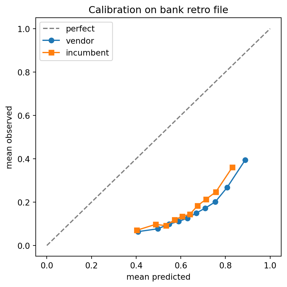
```{python}
import matplotlib.pyplot as plt

fig, ax = plt.subplots(figsize=(5, 5))
ax.plot([0, 1], [0, 1], '--', color='grey', label='perfect')
ax.plot(cal_v['mean_score'], cal_v['mean_y'], 'o-', label='vendor')
cal_i = calibration_table(retro['s_incumbent'], retro['y_default_12m'])
ax.plot(cal_i['mean_score'], cal_i['mean_y'], 's-', label='incumbent')
ax.set_xlabel('mean predicted')
ax.set_ylabel('mean observed')
ax.set_title('Calibration on bank retro file')
ax.legend()
plt.tight_layout()
plt.show()
```
### Swap-set analysis
```{python}
target_approval = 0.70

c_i = np.quantile(retro['s_incumbent'], target_approval)
c_v = np.quantile(retro['s_vendor'], target_approval)

retro['A_i'] = (retro['s_incumbent'] <= c_i).astype(int)
retro['A_v'] = (retro['s_vendor'] <= c_v).astype(int)

confusion = pd.crosstab(retro['A_i'], retro['A_v'])
print('approval matrix (rows incumbent, cols vendor):')
print(confusion)

swap_in = retro[(retro['A_i'] == 0) & (retro['A_v'] == 1)]
swap_out = retro[(retro['A_i'] == 1) & (retro['A_v'] == 0)]

bad_in = swap_in['y_default_12m'].mean()
bad_out = swap_out['y_default_12m'].mean()
print(f"swap-in size:  {len(swap_in)}, bad rate: {bad_in:.4f}")
print(f"swap-out size: {len(swap_out)}, bad rate: {bad_out:.4f}")

r = 600
ell = 4000
profit_in = len(swap_in) * ((1 - bad_in) * r - bad_in * ell)
profit_out = len(swap_out) * ((1 - bad_out) * r - bad_out * ell)
delta_pi = profit_in - profit_out
print(f"swap-in P&L:  ${profit_in:,.0f}")
print(f"swap-out P&L: ${profit_out:,.0f}")
print(f"net delta:    ${delta_pi:,.0f}")
```
### Fair-lending impact
```{python}
def approval_by_group(df, A_col, group_col='group'):
    return df.groupby(group_col)[A_col].mean()

ar_i = approval_by_group(retro, 'A_i')
ar_v = approval_by_group(retro, 'A_v')
print('approval rate by group, incumbent:')
print(ar_i)
print('approval rate by group, vendor:')
print(ar_v)

def air(rates):
    return rates / rates.max()

print('AIR incumbent:')
print(air(ar_i))
print('AIR vendor:')
print(air(ar_v))
```
### Stability
PSI of vendor score on the retro file against a putative vendor-train distribution. Here the vendor-train distribution is simulated as a shifted version of the retro distribution.
```{python}
def psi(reference, production, n_bins=10):
    cuts = np.quantile(reference, np.linspace(0, 1, n_bins + 1))
    cuts[0], cuts[-1] = -np.inf, np.inf
    p_ref, _ = np.histogram(reference, bins=cuts)
    p_prd, _ = np.histogram(production, bins=cuts)
    p_ref = p_ref / p_ref.sum() + 1e-9
    p_prd = p_prd / p_prd.sum() + 1e-9
    return float(np.sum((p_prd - p_ref) * np.log(p_prd / p_ref)))

vendor_train_scores = retro['s_vendor'].values + rng.normal(-0.05, 0.05, N)
vendor_train_scores = np.clip(vendor_train_scores, 0, 1)
print(f"PSI vendor train vs bank back-test: {psi(vendor_train_scores, retro['s_vendor'].values):.4f}")
```
A PSI below 0.1 confirms that the vendor's training distribution is close to the bank's distribution; the bank can adopt the score without re-calibration. Above 0.2, re-calibration on the bank's retro file is required.
---
## The standard library call {#sec-ch34b-lib}
A production back-test uses sklearn for metrics, statsmodels for the calibration regression, and a paired bootstrap from `scipy` or `arch`. The from-scratch DeLong above is replaced by `bench.py` style helpers; many teams maintain an internal `backtest_kit` package.
```{python}
from sklearn.metrics import roc_curve, brier_score_loss
from sklearn.linear_model import LogisticRegression
from sklearn.isotonic import IsotonicRegression

brier_v = brier_score_loss(retro['y_default_12m'], retro['s_vendor'])
print(f"Vendor Brier: {brier_v:.4f}")

platt = LogisticRegression(max_iter=200)
platt.fit(retro[['s_vendor']], retro['y_default_12m'])
retro['s_vendor_platt'] = platt.predict_proba(retro[['s_vendor']])[:, 1]

iso = IsotonicRegression(out_of_bounds='clip')
iso.fit(retro['s_vendor'], retro['y_default_12m'])
retro['s_vendor_iso'] = iso.predict(retro['s_vendor'])

for name in ['s_vendor', 's_vendor_platt', 's_vendor_iso']:
    cal = calibration_table(retro[name], retro['y_default_12m'])
    ece = (cal['n'] / cal['n'].sum() * (cal['mean_y'] - cal['mean_score']).abs()).sum()
    print(f"{name:>20}: ECE={ece:.4f}")
```
The right calibration choice depends on what the bank intends to use the score for. If the score feeds a regulatory PD, isotonic is preferred because it is non-parametric and respects monotonicity. If the score feeds a downstream linear model, Platt scaling keeps the logit interpretation intact. If the score is used only for ranking (cutoff decisions), calibration matters less and the discrimination test is decisive.
---
## Benchmark on a public dataset {#sec-ch34b-bench}
To stay reproducible, replace the simulated retro file with the Taiwan default panel from @sec-ch04. Re-run the back-test framework with two scorers: a baseline logistic and a gradient boosting model. Treat the logistic as the bank's incumbent, the boosting as the vendor.
```{python}
import sys, pathlib
sys.path.insert(0, str(pathlib.Path().resolve().parent / "book" / "code"))
sys.path.insert(0, str(pathlib.Path().resolve() / "code"))
from creditutils import load_taiwan_default
from sklearn.model_selection import train_test_split
from sklearn.linear_model import LogisticRegression
from sklearn.ensemble import GradientBoostingClassifier
from sklearn.preprocessing import StandardScaler
from sklearn.pipeline import Pipeline

taiwan = load_taiwan_default()
y = taiwan['default'].astype(int)
X = taiwan.drop(columns=['default', 'id'])

X_train, X_test, y_train, y_test = train_test_split(X, y, test_size=0.4, random_state=42, stratify=y)

incumbent = Pipeline([('scale', StandardScaler()), ('lr', LogisticRegression(max_iter=200))])
incumbent.fit(X_train, y_train)
s_i = incumbent.predict_proba(X_test)[:, 1]

vendor = GradientBoostingClassifier(n_estimators=150, max_depth=3, random_state=0)
vendor.fit(X_train, y_train)
s_v = vendor.predict_proba(X_test)[:, 1]

auc_i = roc_auc_score(y_test, s_i)
auc_v = roc_auc_score(y_test, s_v)
print(f"Taiwan AUC: incumbent {auc_i:.4f}, vendor {auc_v:.4f}, delta {auc_v - auc_i:+.4f}")

c_i = np.quantile(s_i, 0.30)
c_v = np.quantile(s_v, 0.30)

import pandas as pd
panel = pd.DataFrame({'y': y_test.values, 's_i': s_i, 's_v': s_v})
panel['A_i'] = (panel['s_i'] <= c_i).astype(int)
panel['A_v'] = (panel['s_v'] <= c_v).astype(int)
swap_in = panel[(panel['A_i'] == 0) & (panel['A_v'] == 1)]
swap_out = panel[(panel['A_i'] == 1) & (panel['A_v'] == 0)]
print(f"Taiwan swap-in: n={len(swap_in)}, bad={swap_in['y'].mean():.4f}")
print(f"Taiwan swap-out: n={len(swap_out)}, bad={swap_out['y'].mean():.4f}")
```
The Taiwan benchmark gives a numeric anchor: on this dataset a properly tuned gradient boosting model beats a regularized logistic by roughly 0.02 to 0.04 AUC. The swap analysis converts that uplift into an approve-set composition change. A bank that adopts the boosting model in place of the logistic at the same approval rate sees a measurable reduction in the bad rate of swapped-in applicants.
The same template, applied to a real engagement, takes a week to a fortnight from receipt of retro file to back-test report. The bottleneck is rarely modeling; it is data quality on the retro file and the customer-match step.
---
## Pricing and commercial terms {#sec-ch34b-pricing}
The pricing model is where the analytic back-test meets the commercial reality. Three structures dominate.
**Per-pull (per-scored-application).** The bank pays a fixed price per scored application, typically 0.05 to 0.50 USD for a bureau-style score in mature markets, 0.10 to 1.50 USD for a richer alternative-data score, and 1.00 to 5.00 USD for SME or commercial scores that involve manual data enrichment. Per-pull pricing scales linearly with volume and is the default for high-volume retail use cases. The vendor's revenue is volatile in this structure; the bank's cost is predictable.
**Subscription with volume commitment.** The bank commits to a minimum monthly or annual volume at a discounted per-pull rate, with overage at a published rate. Subscriptions are the dominant model for mid-volume banks that want predictable cost. The vendor's revenue is predictable in this structure; the bank gives up the option to scale down without penalty.
**Revenue or savings share.** The vendor's price is a share of the incremental profit (or savings) the score generates against an agreed baseline. The structure aligns incentives but is operationally heavy: measuring incremental profit requires the swap-set analysis to be re-run every quarter against a frozen baseline. Used by a small number of vendors selling into emerging-market lenders where the bank cannot afford fixed per-pull pricing.
The price card is rarely a single number. It varies by score type (origination, behavioral, collections), by volume tier, by add-on (reason codes, monitoring, retraining cadence, model cards in vernacular), by commitment length, and by exclusivity. The vendor sales motion is to up-sell from a base origination score to a portfolio of scores; the bank's procurement motion is to bundle multiple scores into a single discount tier.
### Service-level agreement
The SLA governs operational behavior. The standard clauses:
- **Availability.** 99.9 percent uptime monthly for online scoring, with named-service-credit penalties for breach. 99.99 percent is the premium tier.
- **Latency.** p99 response time under 200 ms for online scoring on a retail application payload. Batch SLAs are looser, often 24 hours for an overnight job.
- **Score stability.** No more than a stated PSI shift in scores over a rolling period without prior notice and re-validation. Typical clause: PSI above 0.1 triggers a notification, above 0.2 triggers a joint review, above 0.25 voids the SLA pending remediation.
- **Performance maintenance.** The vendor commits to a floor AUC (relative to the back-test) over the contract term. AUC drop beyond a stated threshold triggers a remediation right.
- **Model change control.** The vendor cannot retrain the score without notice. Typical clause: 90 days notice plus a joint re-validation before the new model goes live.
- **Data residency.** The bank's data is processed in a specified jurisdiction. Cross-border processing requires a documented transfer-impact assessment.
- **Audit rights.** The bank or its regulator may audit the vendor's controls annually. The vendor delivers a SOC 2 Type II report or equivalent on a stated cadence.
Indemnification is the most contested clause. The vendor's liability for a fair-lending or FCRA breach attributable to the score itself is typically capped at one to three years of fees. The bank wants uncapped liability for gross negligence. The compromise position is uncapped liability for willful misconduct, capped liability for ordinary negligence, with the cap stepping up over the contract term.
### Pricing-against-back-test arithmetic
The bank's procurement team converts the swap-set P&L into a per-pull break-even price. If the swap analysis shows an incremental P&L of $N$ million USD per year on $V$ million applications, the break-even per-pull price is $N / V$ USD. The vendor's asking price has to leave a margin of safety for the bank: typical procurement rule is the vendor price should not exceed 30 to 50 percent of the calculated per-pull P&L uplift. A vendor that asks 80 percent of the lift is asking the bank to take operational risk for no margin.
### Most-favored-nation and price-protection clauses
Banks at the top of the volume tier typically negotiate a most-favored-nation (MFN) clause: the vendor agrees that the price the bank pays is no higher than the price paid by any comparable client (same volume tier, same product, same geography). MFN is hard to administer and even harder to enforce; vendors typically resist a full MFN and concede a softer variant, the "benchmark refresh" clause, where the bank can request a price review every 12 to 18 months and the vendor commits to either match a published benchmark or document why its product is differentiated. The benchmark-refresh path is more sustainable than full MFN and is the dominant compromise in mature procurement contracts.
Price-protection clauses pin the per-pull price for the contract term against general inflation, against competitive pressure, and against the vendor's own price-card updates. A typical clause: the per-pull price is fixed for the first 24 months, may rise by no more than CPI for months 25 through 36, and is renegotiated at renewal. Without price protection, the vendor can issue a new price card mid-contract and shift the economics; banks that learn this the hard way insist on price protection in every subsequent contract.
### Exit terms and data-return
Exit terms are often the most under-negotiated clauses in the contract and the most expensive to fix later. The standard set covers a wind-down window (typically 12 months from notice), continued scoring at contract rates during the wind-down, return or destruction of bank data, return of the scoring artifacts that the bank has integrated against (including the calibration map and the reason-code taxonomy), and a transition-services commitment to support replacement. A vendor that resists a clean exit clause is a vendor whose contract is operationally lock-in, regardless of what the marketing deck claims.
### Pilot pricing and right-sized commitments
For the POC and pilot stages of @sec-ch34b-lifecycle, banks rarely commit to volume. The pricing structure for pilots is typically a fixed engagement fee covering the back-test work, plus a per-pull rate for the shadow window, with a credit toward the production contract if signed. The pilot fee covers the vendor's data-engineering cost for the retro-file scoring and the back-test report. Banks that demand free pilots are getting either a low-quality back-test or a vendor cross-subsidizing from other clients; either is a procurement risk and the bank should pay a fair pilot fee to get a real test.
---
## Scalability {#sec-ch34b-scale}
Vendor back-tests scale in two dimensions: per-bank (the retro file gets larger as the bank's history grows) and across banks (the vendor runs the same protocol with dozens of bank clients in parallel).
Within a single retro file, the binding workloads are the customer match, the score computation, and the back-test report. The match is typically the slowest: fuzzy matching at scale uses locality-sensitive hashing on n-gram shingles [@broder1997syntactic] and parallel comparison in Dask or Spark. Pandas handles retro files up to roughly 5 million rows in memory; beyond that, Polars or Dask is the standard. PySpark is reserved for retro files that include high-cardinality categorical features (merchant categories, device types) and that exceed a single-machine workflow.
Across banks, the vendor needs to keep client retro files strictly isolated. The compliance reason is obvious: bank A's data cannot mingle with bank B's. The engineering reason is that the back-test results must be reproducible per bank; a shared compute environment that leaks state across clients can produce non-deterministic results. The standard pattern is per-client compute namespaces (separate Kubernetes namespaces or separate VPCs in cloud) with cryptographic key separation. MLflow tracking servers are per-client; experiment results are not commingled.
A second cross-bank consideration is the meta-evaluation. The vendor wants to know how its score performs across the entire client base, not just one bank. A meta-evaluation aggregates the per-bank back-test reports into a portfolio view, with anonymization controls so that no client's results are identifiable. The meta-evaluation is the input to the vendor's own model-improvement roadmap: if the score consistently underperforms on emerging-market clients, the next development cycle targets that segment.
### Compute budget for a back-test
A representative back-test on a 200,000-row retro file with 50 features and the metrics in @sec-ch34b-perf takes about 12 to 25 minutes of wall-clock on a 16-core laptop with Polars. The DeLong test on 5,000-row subsamples runs in seconds; on the full 200,000 rows the O(n^2) inner loop is the bottleneck and the test is replaced by a batched implementation that vectorizes the ranking. A 5-million row retro file moves the workflow to Dask or Spark; the dominant cost is the bootstrap resampling (1,000 replicates) rather than the metric computation itself. Banks running quarterly back-tests automate the entire flow with a Makefile or an Airflow DAG and budget two to three engineer-weeks per year per vendor for back-test maintenance.
### Parallelism in the bootstrap
The block bootstrap dominates compute time in any back-test report. The naive serial implementation runs 1,000 replicates sequentially; on a multi-core machine, each replicate is independent and trivially parallelizable. `joblib.Parallel` with `n_jobs=-1` gives near-linear speedup up to the number of physical cores. For larger replicate counts (10,000 for tail probabilities), the cluster-scale version uses Dask's `delayed` graph; for cloud deployments the AWS Batch or GCP Cloud Run Jobs pattern is sufficient. The block bootstrap's block-size sensitivity should be tested by re-running with block sizes of 1, 2, 4, and 8 vintage months and confirming the confidence intervals are stable.
---
## Deployment {#sec-ch34b-deploy}
The deployment surface for a vendor score is narrower than the deployment surface for an internal model. The vendor exposes a scoring endpoint (REST, gRPC, or batch SFTP) and a small set of management endpoints (health, version, reason-code lookup). The bank consumes the endpoint from its decision engine. The integration surface is small by design; everything else is a contract obligation rather than a code obligation.
A minimal scoring envelope. The bank sends a JSON payload of features; the vendor returns a score, a version, a reason-code list, and an audit ID. The audit ID is the foreign key into the vendor's scoring log; the bank uses it to retrieve scoring evidence if the score is challenged in court or in an adverse-action dispute.
```python
{
  "score": 0.0832,
  "version": "vendor-score-v3.2.1",
  "calibration": "platt-bank-XYZ-2026q1",
  "reason_codes": ["high_utilization", "recent_delinquency", "short_tenure"],
  "audit_id": "vs-2026-05-15-abc123def456"
}
```
The vendor's audit trail is a regulated artifact. Under FCRA, the vendor as a consumer reporting agency (or affiliate) must retain scoring records for a stated period [@fcra1970]. Under GDPR Article 22 and the EU AI Act, the vendor as a provider of a high-risk AI system must keep automatically generated logs for the duration of the system's lifecycle [@eu2016gdpr; @eu_ai_act_2024]. The audit log is queryable by the bank with proper authorization and by the regulator on demand.
Monitoring is split. The vendor monitors the score distribution, latency, and availability across all clients. The bank monitors the score's behavior in its own decision engine: how often is the score used, what is the override rate, what is the back-test performance on each new vintage. The two monitoring layers are stitched together by the audit ID and by a shared incident-response runbook.
A specific deployment pattern that has worked at multiple Vietnamese fintech-bank partnerships: the vendor stands up a scoring sidecar inside the bank's VPC (data residency satisfied), the sidecar pulls the model artifact and the calibration map from the vendor's cloud at startup over a mTLS channel, scoring happens entirely inside the bank's VPC, and only telemetry (no PII, no scores) flows back to the vendor's monitoring stack. Decree 53/2022 on data localization [@vn_decree53_2022] is satisfied by the sidecar pattern; Decree 13/2023 personal-data rules are satisfied by the no-PII telemetry contract [@vn_decree13_2023].
### Version pinning and rollback
The bank consumes a specific version of the vendor's model. The contract pins that version: a new model version cannot be deployed without notice and re-validation. The integration enforces the pin by reading the version field from every score response and rejecting unexpected values. A bank that does not pin the version learns the hard way that the vendor's CI/CD pipeline pushed a new artifact silently and the decision engine started scoring on a model the bank had never seen.
Rollback is the other side of pinning. The integration retains the prior version's scoring artifact (or a remote endpoint to the prior version) for a stated rollback window of typically 30 to 60 days. If a production anomaly is traced to the new version, the decision engine switches traffic back to the prior version within minutes. The rollback is a contract right and an integration capability, not a vague commitment. Vendors who cannot demonstrate a rollback path in the POC stage are deployment risks.
### Monitoring SLAs
The monitoring SLA is the lived form of the back-test charter. It enumerates the metrics monitored in production (PSI on the score distribution, PSI per feature, AUC on rolling vintages once outcomes mature, override rate, latency p50/p95/p99, error rate), the thresholds that trigger alerts, the parties notified (vendor on-call, bank on-call, joint incident channel), the escalation path, and the post-incident review cadence. A monitoring SLA without named thresholds is decorative; what matters is the specific number that triggers a page and the specific runbook that follows.
The monitoring data flows back to the back-test charter at renewal. The cumulative production AUC across vintages is the empirical answer to whether the back-test predicted production well. A 0.02 back-test uplift that materializes as 0.018 production uplift is a successful vendor; a 0.02 back-test uplift that materializes as 0.008 production uplift is a vendor whose retraining clause is about to be exercised.
---
## Regulatory considerations {#sec-ch34b-reg}
A vendor selling a credit score into a regulated bank sits inside three overlapping regimes: prudential model risk (SR 11-7 and equivalents), consumer protection (ECOA Regulation B, FCRA, GDPR Article 22, EU AI Act, local consumer-credit laws), and third-party risk management (joint interagency 2023 guidance in the US, EBA guidelines in the EU, SBV Circular 13/2018 in Vietnam).
### SR 11-7 and third-party model risk
SR 11-7 [@fed2011sr117] treats vendor models the same as in-house models. The bank as model owner is responsible for conceptual soundness, ongoing monitoring, and outcomes analysis. The vendor's role is to supply the artifacts the bank needs to satisfy those duties. In practice this means the vendor delivers a model card to SR 11-7 standard: data sources, sampling design, target definition, feature engineering, model class and hyper-parameters, performance on development sample, fair-lending position, monitoring plan, known limitations. The bank's model risk management function reviews the card and gates adoption.
The 2023 joint interagency guidance on third-party risk management [@feb2023_3rdparty] tightened the expectations. The bank's third-party risk function is responsible for due diligence (financial health, security posture, compliance history), contracting (clear allocation of responsibilities), ongoing monitoring (performance, incident response, change management), and termination (orderly exit, data return, post-termination obligations). The model risk function and the third-party risk function jointly own a vendor score; neither is sufficient alone.
### FCRA and reseller liability
In the US, a vendor score derived from consumer-report data is itself a consumer-report-related output under FCRA [@fcra1970]. The vendor may be a consumer reporting agency (if it furnishes information to others) or a reseller (if it repackages bureau data). Either status carries permissible-purpose duties, accuracy requirements, dispute-handling obligations, and identity-verification controls. A bank that uses a score for an adverse-action decision must be able to disclose the source of the score and the key factors that affected it [@cfpb2013ecoa]. The vendor contract must include a covenant that the vendor will support adverse-action notice generation, including specific reason codes that comply with the CFPB's adverse-action requirements [@cfpb2022_circ_2202_03].
### ECOA Regulation B
Regulation B prohibits discrimination on a prohibited basis and requires adverse-action notices specify principal reasons. The CFPB has clarified that "complex algorithms" do not relieve creditors of the specificity duty [@cfpb2022_circ_2202_03]. A score that returns only a probability and a generic "credit characteristics" reason will fail Regulation B compliance review. The vendor must supply reason codes that the bank can map to applicant-facing language.
### EU AI Act
Credit scoring is classified as a high-risk AI system under Annex III of the EU AI Act [@eu_ai_act_2024]. The vendor as provider of a high-risk system is responsible for risk management, data governance, technical documentation, transparency, human oversight, accuracy, robustness, and cybersecurity. The bank as deployer is responsible for operating the system per the provider's instructions, monitoring, and incident reporting. The provider-deployer split mirrors the SR 11-7 model-owner-vendor split but with sharper teeth: misclassification of the role carries direct regulatory liability. The vendor contract for an EU deployment must allocate the provider role clearly and include the technical documentation set required by Article 11 and Annex IV.
### GDPR Article 22 and DPIA
Under GDPR Article 22 [@eu2016gdpr], a credit decision based solely on automated processing is allowed only with explicit consent, contractual necessity, or Union/Member State law authorization, and only with safeguards including the right to human review. A vendor score that drives an automated decline triggers the safeguards. A Data Protection Impact Assessment (Article 35) is required before deployment; the vendor supplies the technical inputs.
### Local regimes: Vietnam, Singapore, Indonesia
Vietnam's Decree 13/2023 [@vn_decree13_2023] is the consent regime; Decree 53/2022 [@vn_decree53_2022] is the data-localization regime; Decree 94/2025 [@vn_decree94_2025] is the fintech sandbox regime. A vendor selling into a Vietnamese bank must satisfy all three: consent record at the bank application, scoring inside Vietnam (sidecar pattern from @sec-ch34b-deploy), and sandbox enrollment if the use case is novel. Singapore's PDPA and MAS notices on technology risk and outsourcing govern equivalent issues; Indonesia's UU PDP and OJK fintech-lending rules govern the Indonesian path. The vendor's compliance posture must be jurisdiction-specific; a single global compliance posture is not enough.
---
## Vietnam case study {#sec-ch34b-vietnam}
A composite case study, anonymized but drawn from multiple Vietnamese score-vendor deployments over 2022 to 2025. A consumer-finance company (CFC) with a thin-file mass-market portfolio wanted to replace its in-house origination scorecard, which had been built on CIC bureau pulls and basic application fields, with an alternative-data-enriched score from a regional fintech vendor.
**Stage 1 (RFI).** The CFC issued an RFI to four vendors. Two were CIC-affiliated and offered bureau-enriched scores; two were alternative-data vendors with telco and e-wallet feeds. All four submitted decks; two were invited to RFP.
**Stage 2 (RFP and NDA).** Both finalists signed mutual NDAs and submitted detailed responses. The alternative-data vendor disclosed its training-data composition (60 percent Vietnamese, 25 percent Thai, 15 percent Indonesian) and its target segment (thin-file consumer finance, 18 to 35 year olds). The bureau-enriched vendor disclosed CIC and PCB data licensing arrangements.
**Stage 3 (POC).** The CFC delivered a retro file of 120,000 applications from 2022 to 2023 vintages, with 12-month performance attached. Surrogate IDs were SHA-256 hashes of the application number with a per-deal salt. The bureau-enriched vendor matched 91 percent of rows via hashed national ID; the alternative-data vendor matched 73 percent via a fuzzy name-DOB-phone match. The CFC ran the back-test framework from this chapter on both. The bureau-enriched vendor delivered a 0.024 AUC uplift over the incumbent with $p < 0.01$ on paired DeLong, ECE of 0.018 after Platt scaling, and a swap-set P&L of approximately 8 percent of incumbent profit. The alternative-data vendor delivered a 0.018 AUC uplift, ECE of 0.034, and a swap-set P&L of 12 percent, but with a 22 percent unmatched cohort that had to be scored by the incumbent only.
**Stage 4 (commercial).** The CFC chose the alternative-data vendor on the strength of the swap-set P&L and the segment fit, despite the lower AUC uplift. The contract was structured as a per-pull subscription with a volume commitment and a quarterly retraining cadence; the vendor agreed to a no-material-change clause with 90 days notice. Data residency was Vietnam (sidecar pattern); cross-border telemetry was anonymized aggregate only.
**Stage 5 (shadow).** Sixty days of shadow scoring on live applications, with the vendor score logged but not used in decisions. Production AUC tracked the back-test AUC within 0.005; PSI of vendor train versus production stayed below 0.12. The CFC's model risk function signed off.
**Stage 6 (go-live).** Rollout from 10 percent traffic to 100 percent over 90 days, with model risk management sign-off at each step. By month four, the CFC was scoring 100 percent of new applications with the vendor score; the incumbent moved to a back-up role.
**Stage 7 (monitoring).** Quarterly back-test refresh on the new vintage. Year-one performance came in at 0.020 AUC uplift (slightly below back-test), ECE 0.025, swap-set P&L 9 percent of incumbent. AIR by gender (the only protected class consistently captured at application) stayed above 0.85 throughout. Year-two performance dropped to 0.014 AUC uplift after a macro tightening; the contract's remediation clause was invoked and the vendor delivered a retrained variant in month 18 of the term that restored the uplift to 0.021.
Three lessons from the case. First, the alternative-data vendor lost on AUC but won on swap-set P&L because the segment overlap with the CFC's thin-file portfolio was tighter than the bureau-enriched vendor's coverage. The metric that mattered was operational lift, not the headline AUC. Second, the retraining clause was load-bearing: without it the year-two AUC drop would have triggered an unscheduled procurement cycle that would have cost the CFC six to nine months of optionality. Third, the data-residency requirement under Decree 53/2022 cost the vendor roughly four to six weeks of integration work but did not materially change the back-test result, because the sidecar pattern keeps the modeling and scoring logic identical to the offshore reference deployment.
### A second Vietnam mini-case: BNPL partnership
A separate engagement, contemporaneous with the CFC case, involved a domestic BNPL platform selling its merchant-side risk score to a partner bank for the bank's own unsecured personal-loan portfolio. The structural inversion is interesting: the BNPL platform held the score, the bank held the loan-of-record, and the score was being used to cross-underwrite a different product than the one the score was trained on.
The retro file in this case was the bank's existing personal-loan applications from 2022 and 2023. The BNPL platform matched on hashed national ID with a 67 percent hit rate. The hit rate was lower than the CFC case because the BNPL platform's coverage was concentrated in younger urban consumers; the bank's personal-loan applicant pool skewed older and more provincial. The back-test on matched rows showed a 0.031 AUC uplift over the bank's incumbent on younger urban applicants and roughly zero uplift on older provincial applicants. The aggregate AUC uplift was 0.011, which fell below the bank's pre-registered 0.02 threshold.
The bank could have rejected the score on the aggregate result. It did not, because the segment-stratified back-test (see @sec-ch34b-perf for the framework) showed that the vendor's lift on the younger urban segment was strong and durable across two vintages. The procurement decision was to use the score as a segment-specific overlay: for the bank's younger urban segment (roughly 22 percent of applicants), the BNPL score served as a second opinion alongside the incumbent; for the rest of the book, the incumbent ran alone. Per-pull pricing reflected the narrower scope.
This case illustrates a principle that the headline AUC obscures: a vendor score that fails an aggregate threshold can still be a profitable procurement if the segment lift is real and the bank is willing to architect a segment-specific deployment. The procurement decision is jointly about the score quality and the bank's operational capacity to deploy it on the right slice of traffic.
### A counterfactual: the deal that should not have closed
A third anonymized example from the same market period. A regional bank ran an RFI, RFP, and POC with a US-domiciled alternative-data vendor whose Asia coverage was limited. The vendor's headline AUC on Vietnamese data was strong (the back-test showed 0.026 uplift), but the segment analysis revealed the lift was concentrated in the top decile and reversed in the bottom four deciles. The PSI of vendor train to Vietnam back-test was 0.34, well above the 0.2 threshold. The vendor's marketing material did not disclose the training distribution; the model card produced for the POC named only that the training data was "primarily North American consumer."
The bank's model risk function flagged the PSI and the segment reversal. The vendor offered a re-calibration on the Vietnamese retro file, which it positioned as a routine deployment step. The risk function pointed out that a re-calibration on a sample with PSI 0.34 against the training population was effectively a re-training in disguise, and a re-training that the vendor had not validated against its development sample standards. The deal did not close. The bank issued a follow-up RFP six months later to vendors with documented Asia training coverage.
The counterfactual matters because the bank's commercial team had been ready to sign. The procurement gates around back-test charters, PSI thresholds, and model-card disclosures are what stopped a marginal deal from progressing. A practitioner reading the back-test report can see the warning signs in five minutes; without the pre-registered thresholds, the same report reads as a successful POC.
---
## Operational risk and incident response {#sec-ch34b-incident}
A vendor score is an operational risk surface. Three classes of incident recur.
**Scoring-pipeline incident.** The vendor's endpoint fails, returns errors, or returns degraded scores. The bank's decision engine must fail gracefully: typical pattern is a fallback to the incumbent score with an override flag, plus an alert to the joint incident channel. The fallback path must itself be tested quarterly; banks that maintain the fallback as a write-only artifact discover at the worst moment that it is not actually wired up.
**Data-pipeline incident.** A bank-side feature pipeline breaks (a bureau pull times out, a feature store deploys a buggy transformation). The vendor receives partial features, returns a score conditioned on incomplete data, and the score is silently wrong. The mitigation is feature-completeness checks at the integration boundary: every score request validates that every required feature is non-null and within expected ranges; missing or out-of-range features trigger a routing decision (use a backup score, route to manual review, or decline with a clean reason code). The vendor and bank agree on the validation schema at integration time.
**Model-drift incident.** Performance degrades over weeks or months without an acute trigger. The monitoring stack catches it through PSI shift, override-rate increase, or rolling-vintage AUC decline. The contract specifies the remediation: investigation by the vendor within a stated window, joint review, retraining or recalibration as needed. The hardest incidents in this class are those where drift is asymmetric across segments; the aggregate metric stays inside SLA but a specific segment is failing. Segment-level monitoring (the same stratification as @sec-ch34b-perf) is what catches these.
The incident-response runbook is a deliverable in the procurement package. A vendor that ships a model without a documented runbook is shipping deployment risk; the bank's third-party risk function will block the deal until the runbook is delivered and tested in a tabletop exercise.
### Insurance and indemnification mechanics
For large deployments, the bank may require the vendor to carry errors and omissions (E&O) and cyber-liability insurance, with policy limits commensurate with the bank's exposure. The vendor's general liability cap negotiated in the indemnification clause is independent of the insurance coverage; the insurance is a credit-enhancement on the indemnification, not a substitute. A vendor that resists insurance disclosure is a vendor whose financial backing is thin, which is itself a third-party risk consideration.
## Takeaways {#sec-ch34b-takeaways}
- The retro file is the artifact that decides a vendor sale. Build it with the same point-in-time discipline as an internal model validation. A retro file that leaks future information overstates the back-test by more than any plausible AUC uplift the vendor can deliver.
- AUC is necessary, not sufficient. The swap-set P&L converts statistical lift into procurement-grade evidence and is the metric that closes deals. Pre-register a profit threshold before the data crosses, not after.
- Customer matching is the most under-engineered step in the protocol. Hit rate, match quality, and lift on matched are first-class metrics; report them alongside AUC.
- Fair-lending impact is not optional. AIR at the proposed cutoffs is a release gate. The contract must specify the remediation path if AIR fails.
- Pricing follows the back-test. The break-even per-pull price falls out of the swap-set P&L; the vendor's ask should leave the bank a margin of safety of two to three times the integration risk.
- The vendor's regulatory posture must be jurisdiction-specific. SR 11-7 plus FCRA plus Regulation B is the US baseline; EU AI Act provider duties plus GDPR DPIA is the EU baseline; Decree 13/2023 plus Decree 53/2022 plus Decree 94/2025 is the Vietnam baseline. A single global compliance posture is not enough.
- Sidecar deployment satisfies data-residency rules without forcing the vendor to re-engineer the model. It is the dominant pattern in regulated emerging-market deployments and is increasingly common in EU jurisdictions with national data-protection variants.
---
## Further reading {#sec-ch34b-further}
- @fed2011sr117 on supervisory expectations for model risk management.
- @occ2011handbook for the equivalent OCC handbook.
- @pra2023ss123 for the PRA principles for model risk management.
- @feb2023_3rdparty for the 2023 US interagency guidance on third-party risk management.
- @delong1988comparing for the paired ROC comparison test.
- @hosmer2013applied for the standard reference on applied logistic regression and calibration tests.
- @platt1999probabilistic and @niculescu2005predicting for calibration methods.
- @broder1997syntactic on locality-sensitive hashing for entity resolution.
- @elliott2009using and @cfpb2014bisg on Bayesian Improved Surname Geocoding for proxy race estimation.
- @cfpb2022_circ_2202_03 on adverse-action specificity for complex algorithms.
- @eu_ai_act_2024 for the EU AI Act and its provider/deployer split.
- @vn_decree13_2023, @vn_decree53_2022, @vn_decree94_2025 for the Vietnamese data and sandbox regime.
- @hand1997statistical and @hand2001measuring for the foundational treatment of scorecard construction and measurement.
- @basel2006international and @bcbs355 on third-party model treatment under Basel.