---
execute:
echo: true
eval: true
bibliography: ["../references.bib", "../refs/ch-05.bib"]
---
# Regulatory and Legal Framework {#sec-ch05}
::: {.callout-note appearance="simple" icon="false"}
**Scope: both retail and corporate.** SR 11-7 model risk and Basel IRB apply across portfolios. ECOA, FCRA, GDPR Article 22, and EU AI Act provisions on automated decisions are consumer-specific; ECOA Regulation B also covers small-business credit.
:::
## Overview {.unnumbered}
A credit model is not a mathematical object that merely happens to sit inside a bank. It is a regulated object. Its inputs, training regime, internal parameters, calibration, monitoring, and every adverse decision it issues are bound by overlapping statutes: prudential (Basel, SR 11-7), consumer (ECOA, FCRA), data protection (GDPR), and sectoral AI law (the EU AI Act). A model that earns a higher AUC, but cannot produce a lawful adverse action notice is a model a bank cannot deploy.
This chapter frames the regulatory framework as a set of constraints on the estimator. Each regime maps to precise artifacts: a Pillar I capital number, a reason code string on a notice, a record of an automated decision, a conformity dossier. The methods and code that produce those artifacts sit alongside the estimators that produce the probability of default. Treating them as separable is a common failure mode. We build them jointly.
Why spend an entire chapter on regulation before the first serious estimator? Two reasons. The first is that the constraints are binding. A scorecard architect who does not know that Regulation B §1002.9(b)(2) forbids a generic "failed our internal screening" reason will build a pipeline that cannot be deployed. A modeler who does not know that Basel III §9 imposes an output floor will overestimate the marginal capital benefit of a sophisticated IRB model. A data scientist who does not know that Annex III §5(b) of Regulation (EU) 2024/1689 classifies credit scoring as high-risk will ship a model that requires a conformity assessment and a fundamental-rights impact assessment that have not been built. The failure modes are not statistical; they are legal and operational, and they crystallize the week before launch.
The second is that the regulations shape what is measurable. The Basel IRB definition of default (90 days past due or unlikeliness to pay) is the dependent variable for most PD models at banks. The FCRA definition of a "consumer report" constrains which features enter the model at origination. The GDPR Article 22(3) right to contest means the pipeline must support human review. The EU AI Act Article 14 human oversight requirement means the model is not stand-alone; it is embedded in a workflow that a person can intervene in. Build the estimator without these constraints in mind, and the retrofit is expensive.
The chapter has two halves. The first (@sec-ch05) walks through the Basel IRB capital formula, derives it from the Vasicek asymptotic single-risk-factor (ASRF) model, and implements it in NumPy. The second half covers the law and policy that govern a credit decision once PD is estimated. It includes the Equal Credit Opportunity Act (ECOA) and Regulation B (@sec-ch05-ecoa), the Fair Credit Reporting Act (FCRA) (@sec-ch05-fcra), GDPR Article 22 (@sec-ch05-gdpr), the EU AI Act classification of credit scoring as high-risk (@sec-ch05-euaia), and the U.S. model-risk supervisory guidance SR 11-7 and OCC 2011-12 (@sec-sr117). Adverse action notices, reason-code generation from logistic regression and gradient boosted trees (@sec-adverse-action), and a worked model card complete the chapter.
A word to the emerging-market reader. The Basel, ECOA, FCRA, GDPR, and EU AI Act anchors below are Anglo-American and European, but the substance transplants unevenly. A Vietnamese, Indonesian, Indian, or Nigerian lender operates under a local prudential regime (in Vietnam, SBV Circular 41/2016 for Basel II capital as amended by Circular 22/2023 on capital adequacy ratios, Circular 43/2016 for consumer lending by finance companies, Decree 94/2025 for the fintech sandbox) and a local data-protection regime (in Vietnam, Decree 13/2023 on personal data) that mirror the Western framework in substance while differing in scope, definitions of sensitive data, and adverse-action obligations. The architecture of the chapter, capital formula plus reason codes plus documentation artifacts, is the right architecture anywhere. The specific statutory triggers and the drafting of the reason-code strings are local and are where a cross-border lender has to invest.
One note on scope. The chapter is written from the perspective of a U.S. or EU regulated lender. Many jurisdictions have parallel structures: the UK PRA's SS3/18 on model risk management, the Monetary Authority of Singapore's FEAT principles, the Bank of Canada's E-23 guideline, the Reserve Bank of Australia's CPG 235. These tend to converge on the same substance: IRB-style capital, effective challenge, adverse action or reason-for-decision notices, and an emerging AI-specific overlay. A practitioner in one of those jurisdictions should read the citations here and substitute the local equivalent.
### Notation {.unnumbered}
- $PD$: one-year probability of default for an obligor or facility, expressed as a real number in $[0,1]$.
- $LGD$: loss given default as a fraction of EAD, in $[0,1]$.
- $EAD$: exposure at default, in monetary units.
- $M$: effective maturity of the facility in years (IRB corporate).
- $R$ or $\rho$: asset value correlation.
- $\Phi$ and $\Phi^{-1}$: the standard normal CDF and its inverse.
- $K$: regulatory capital requirement per unit of EAD.
- $RWA$: risk-weighted assets.
- $\mathrm{MoC}$: margin of conservatism.
```{python}
#| echo: true
#| output: false
import sys, json, warnings, time
sys.path.insert(0, "../code")
import numpy as np
import pandas as pd
import matplotlib.pyplot as plt
from scipy.stats import norm
warnings.filterwarnings("ignore")
np.random.seed(7)
from creditutils import load_german_credit
```
## Basel II and III IRB: PD, LGD, EAD, and the ASRF capital formula {#sec-ch05-regulation}
The Internal Ratings Based (IRB) approach under Basel II and its Basel III revisions [@basel2006international; @basel2017finalising] lets a bank use its own estimates of risk parameters to compute regulatory capital. The parameters are $PD$, $LGD$, $EAD$, and (for non-retail exposures) $M$. The capital formula is not a regression fit to data; it is a closed-form consequence of the Vasicek [@vasicek2002loan] asymptotic single-risk-factor (ASRF) model, made portfolio-invariant by Gordy [@gordy2003risk].
### Formal definitions of the IRB parameters
Basel II (paragraphs 452 to 468 of the Comprehensive Version) defines $PD$ as the one-year probability that an obligor will default, conditional on survival to the start of the year. Default itself (paragraph 452) is the later of a 90-days-past-due trigger or a "unlikeliness to pay" assessment. Formally,
$$
PD_i = \Pr\!\left(D_i^{t+1} = 1 \mid \mathcal{F}_t \right),
$$ {#eq-pd-def}
where $D_i^{t+1}$ indicates default of obligor $i$ over the horizon $(t, t+1]$ and $\mathcal{F}_t$ the information set at time $t$. IRB estimates must be long-run averages. Basel II paragraph 447 sets the PD floor for non-retail exposures at 3 basis points (3bps), retained in Basel III [@basel2017finalising §36].
$LGD$ is the facility-level economic loss conditional on default:
$$
LGD_i = \mathbb{E}\!\left[ 1 - \frac{\text{discounted net recoveries}_i}{\text{EAD}_i} \big| D_i = 1 \right].
$$ {#eq-lgd-def}
Economic loss includes direct workout costs, indirect costs, and a discount rate that reflects funding and risk. Basel III caps the retail floor at 25% or less and introduces output floors on LGD; the EBA operationalizes the estimation steps in @eba2017gl.
$EAD$ is the expected exposure at the moment of default. For on-balance-sheet exposures, $EAD$ equals the drawn amount plus a supervisor-set or bank-estimated credit conversion factor (CCF) applied to the undrawn commitment:
$$
EAD_i = \text{Drawn}_i + CCF_i \cdot \text{Undrawn}_i .
$$ {#eq-ead-def}
The effective maturity $M$ for corporate, sovereign, and bank exposures is the cash-flow-weighted average:
$$
M = \frac{\sum_t t \cdot CF_t}{\sum_t CF_t},\qquad 1 \le M \le 5 \text{ years}.
$$ {#eq-maturity}
Retail IRB does not use $M$. Retail exposures are assumed short-term and not subject to maturity mismatch charges. Retail IRB splits into three sub-segments: (i) residential mortgages, (ii) qualifying revolving retail exposures (QRRE, principally credit cards and similar revolving lines), and (iii) "other retail" (auto loans, personal loans, small business loans below the retail threshold). Each sub-segment uses a different asset-value correlation function. The three retail functions are the consequence of Basel II's empirical calibration against observed default correlations; corporate exposures, by contrast, use a PD-dependent correlation that ranges from 0.12 to 0.24.
#### The default definition in practice
Paragraph 452 of Basel II defines default as occurring when at least one of two events has taken place:
1. The bank considers that the obligor is unlikely to pay its credit obligations in full, without recourse to actions such as realizing security.
2. The obligor is past due more than 90 days on any material credit obligation.
The "unlikeliness to pay" (UTP) leg is qualitative and leaves room for supervisory disagreement. Basel II Annex 7 lists indicators: restructuring with economic loss, distressed sale of assets, payment holidays to prevent arrears, bankruptcy filing, specific provisions booked. The EBA guidelines on the application of the default definition (EBA/GL/2016/07) harmonize these indicators across EU banks and introduce a materiality threshold: an absolute materiality threshold (100 EUR retail, 500 EUR non-retail) and a relative threshold (1% of on-balance-sheet exposure).
Counting days past due seems mechanical but is not. The clock starts the day the obligation becomes due and unpaid; it restarts only after the arrears are cured. Technical past-due items (e.g., a payment held in suspense due to processing error, or a disputed charge under FCRA) do not start the clock. The default status must persist for a minimum probation period (EBA: three months for retail, 12 months for unsecured non-retail) after the cure before the obligor can be re-classified as performing. Data pipelines that miss the probation requirement tend to underestimate long-run PDs.
#### LGD: the work beyond the mean
Equation @eq-lgd-def hides considerable operational complexity. The discount rate must reflect the risk of the recovery cash flows, not the risk-free rate. A common practice is to use the original contract rate plus a risk premium; some jurisdictions require the risk-adjusted rate from the bank's internal funds transfer pricing. Workout costs include the salary of the collections staff allocated to the facility, legal fees, and indirect overhead. Indirect costs are typically the hardest to pin down; EBA's 2017 guidelines require that they be included, estimated as a percentage of direct costs if no better measure exists.
Recovery rates on retail loans are often bimodal: a high mass near zero (obligors who repay quickly under hardship programs) and a second mass near one (obligors who charge off fully). Bastos [@bastos2010forecasting] documents this for bank loans; Calabrese and Zenga [@calabrese2014fractional] for Italian consumer loans. A beta regression is a defensible default if the modeler accepts that the mean LGD is a poor summary of the recovery distribution. For downturn LGD the tail of the distribution matters more than the mean, because downturn conditions shift mass from the "recovered" mode to the "charge-off" mode.
#### EAD and off-balance-sheet exposures
For revolving lines, equation @eq-ead-def requires estimating $CCF$ for the undrawn commitment. A CCF of 50% on an undrawn credit card balance means the bank expects half of the available headroom to be drawn between the reporting date and default. For non-retail exposures Basel II provides supervisor-set CCFs (paragraph 311): 75% for commitments with an original maturity over one year, 20% for short-term trade-related contingencies. For advanced IRB retail and non-retail exposures the bank estimates its own CCF or EAD conversion factor.
The Basel III revision [@basel2017finalising §31] removes CCF estimation for retail revolving exposures under the advanced IRB approach and replaces it with supervisor-set numbers for some facilities. This is part of the broader Basel III narrowing of advanced IRB scope; the framework's authors judged that banks' CCF estimates were too optimistic.
### The ASRF model and the capital formula
The Vasicek single-factor structural model takes obligor $i$'s standardized asset return as
$$
A_i = \sqrt{\rho} Y + \sqrt{1 - \rho} \varepsilon_i,\qquad Y,\varepsilon_i \sim \mathcal{N}(0,1) \text{ i.i.d.}
$$ {#eq-asrf-asset}
The obligor defaults when $A_i$ falls below a threshold $c_i = \Phi^{-1}(PD_i)$. Conditional on the systematic factor $Y = y$, the default probability is
$$
p_i(y) = \Phi\!\left(\frac{\Phi^{-1}(PD_i) - \sqrt{\rho} y}{\sqrt{1 - \rho}}\right).
$$ {#eq-asrf-cond}
Gordy [@gordy2003risk] shows that in an infinitely fine-grained, single-factor portfolio the 99.9% VaR of loss is attained by fixing $Y$ at the one-sided 0.1% quantile, $y = -\Phi^{-1}(0.999) = \Phi^{-1}(0.001)$. Substituting,
$$
p_i^{\text{worst}} = \Phi\!\left(\frac{\Phi^{-1}(PD_i) + \sqrt{\rho} \Phi^{-1}(0.999)}{\sqrt{1 - \rho}}\right).
$$ {#eq-asrf-worst}
The unexpected loss per unit of $EAD$, on which IRB capital is charged, is $LGD \cdot (p_i^{\text{worst}} - PD_i)$. For corporate exposures Basel II introduces a maturity adjustment that inflates the charge with $M > 1$:
$$
b(PD) = \bigl(0.11852 - 0.05478 \ln PD\bigr)^2,
$$ {#eq-b-pd}
$$
MA(PD, M) = \frac{1 + (M - 2.5) b(PD)}{1 - 1.5 b(PD)}.
$$ {#eq-maturity-adj}
The Basel II asset value correlation for corporate, sovereign, and bank exposures is
$$
\rho_{\text{corp}}(PD) = 0.12 \cdot \frac{1 - e^{-50 PD}}{1 - e^{-50}} + 0.24 \cdot \left(1 - \frac{1 - e^{-50 PD}}{1 - e^{-50}}\right).
$$ {#eq-rho-corp}
For residential mortgages Basel uses a flat $\rho = 0.15$. For qualifying revolving retail exposures (QRRE, typically credit cards) $\rho = 0.04$. For "other retail" the formula mirrors corporate with a decay constant of 35:
$$
\rho_{\text{other retail}}(PD) = 0.03 \cdot \frac{1 - e^{-35 PD}}{1 - e^{-35}} + 0.16 \cdot \left(1 - \frac{1 - e^{-35 PD}}{1 - e^{-35}}\right).
$$ {#eq-rho-other}
The IRB capital requirement per unit of EAD is then
$$
K(PD, LGD, M) = \left[ LGD \cdot \Phi\!\left(\frac{\Phi^{-1}(PD) + \sqrt{\rho}\, \Phi^{-1}(0.999)}{\sqrt{1 - \rho}}\right) - LGD \cdot PD \right]
\cdot MA(PD, M).
$$ {#eq-irb-k}
Risk-weighted assets are $RWA = K \cdot 12.5 \cdot EAD$, with the $12.5 = 1/0.08$ factor embedding the 8% Basel total-capital ratio. The @bcbs128 explanatory note derives each element of this formula from the Vasicek model.
Three properties of the formula deserve attention.
**Portfolio invariance**. Gordy's key theoretical contribution [@gordy2003risk] is that in the infinitely fine-grained limit the 99.9% VaR is a sum of contributions, each of which depends only on the obligor's own parameters ($PD_i$, $LGD_i$, $M_i$, $EAD_i$) and the systematic factor. No cross-obligor interaction term survives. This is what lets Basel set capital per facility rather than per portfolio. The trade-off is that idiosyncratic concentration risk, sectoral concentration risk, and double default risk are lost; they re-enter through Pillar II add-ons.
**Inelasticity at the extremes**. Because $\rho$ is a convex combination of two constants as a function of $PD$ (through the weighting function $w$), the correlation approaches $0.24$ as $PD \to 0$ and $0.12$ as $PD \to 1$ for corporate exposures. In the retail formulas the analogous limits are 0.16 and 0.03. The effect is that low-$PD$ obligors have higher correlation and therefore disproportionately higher capital per unit of expected loss. The Basel committee's rationale is that a small shock to a highly-rated obligor (a downgrade that moves $PD$ from 10bps to 100bps) is likely to be systemic; obligors already rated as high-risk have default probabilities driven more by idiosyncratic stress.
**No cycle dependence in the formula itself**. The IRB formula takes $PD$ as given; the cycle dependence enters through the bank's choice of rating philosophy. A "through-the-cycle" (TTC) PD is designed to be stable across the business cycle; a "point-in-time" (PIT) PD reflects current economic conditions and moves with the cycle. A TTC PD plugged into the IRB formula yields stable capital charges; a PIT PD yields capital that rises in recessions. The Basel framework permits either, but supervisors scrutinize the stability of capital under stress. In practice many banks use a hybrid rating philosophy, and the rating philosophy must be disclosed and documented under SR 11-7.
### Implementation from scratch and retail vs corporate comparison
```{python}
#| label: fig-irb-capital
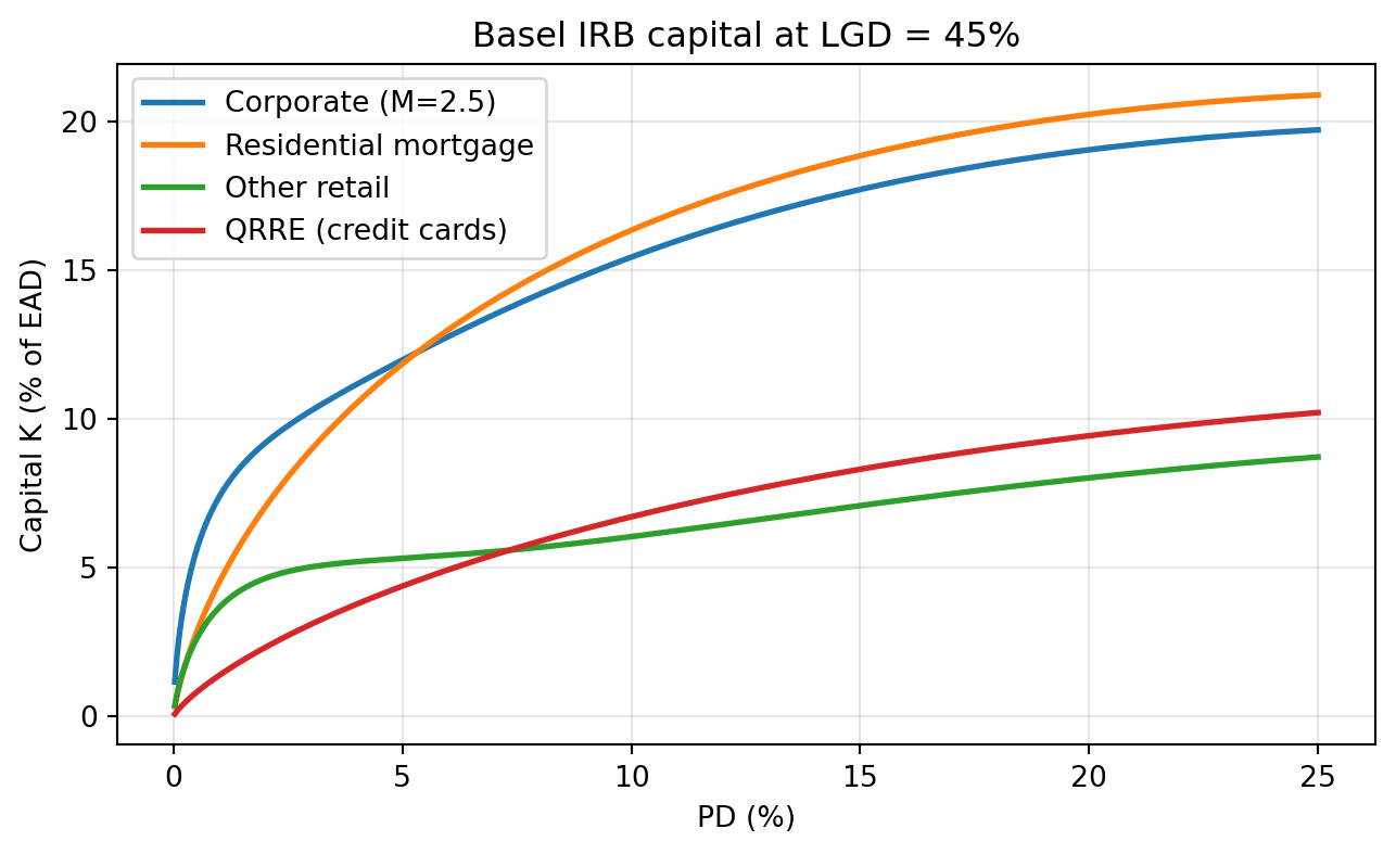
#| fig-cap: "IRB capital K(PD) at LGD=45% for corporate (M=2.5), residential mortgage (rho=0.15), and other retail exposures."
def rho_corporate(pd_):
    """Basel II corporate/sovereign/bank asset-value correlation."""
    pd_ = np.clip(np.asarray(pd_, float), 1e-6, 0.9999)
    w = (1.0 - np.exp(-50.0 * pd_)) / (1.0 - np.exp(-50.0))
    return 0.12 * w + 0.24 * (1.0 - w)

def rho_other_retail(pd_):
    pd_ = np.clip(np.asarray(pd_, float), 1e-6, 0.9999)
    w = (1.0 - np.exp(-35.0 * pd_)) / (1.0 - np.exp(-35.0))
    return 0.03 * w + 0.16 * (1.0 - w)

def rho_qrre(pd_):
    return np.full_like(np.asarray(pd_, float), 0.04)

def rho_mortgage(pd_):
    return np.full_like(np.asarray(pd_, float), 0.15)

def maturity_adjustment(pd_, M=2.5):
    pd_ = np.clip(np.asarray(pd_, float), 1e-6, 0.9999)
    b = (0.11852 - 0.05478 * np.log(pd_)) ** 2
    return (1.0 + (M - 2.5) * b) / (1.0 - 1.5 * b)

def K_irb(pd_, lgd=0.45, rho_fn=rho_corporate, M=None):
    """Capital per unit EAD under the Basel IRB formula."""
    pd_ = np.clip(np.asarray(pd_, float), 1e-6, 0.9999)
    rho = rho_fn(pd_)
    q = norm.ppf(0.999)
    worst = norm.cdf((norm.ppf(pd_) + np.sqrt(rho) * q) / np.sqrt(1.0 - rho))
    k = lgd * (worst - pd_)
    if M is not None:
        k = k * maturity_adjustment(pd_, M)
    return k

pds = np.geomspace(3e-4, 0.25, 200)
K_corp = K_irb(pds, 0.45, rho_corporate, M=2.5)
K_mort = K_irb(pds, 0.45, rho_mortgage)
K_oret = K_irb(pds, 0.45, rho_other_retail)
K_qrre = K_irb(pds, 0.45, rho_qrre)

fig, ax = plt.subplots(figsize=(6.8, 4.2))
ax.plot(pds * 100, K_corp * 100, label="Corporate (M=2.5)", lw=2)
ax.plot(pds * 100, K_mort * 100, label="Residential mortgage", lw=2)
ax.plot(pds * 100, K_oret * 100, label="Other retail", lw=2)
ax.plot(pds * 100, K_qrre * 100, label="QRRE (credit cards)", lw=2)
ax.set_xlabel("PD (%)"); ax.set_ylabel("Capital K (% of EAD)")
ax.set_title("Basel IRB capital at LGD = 45%")
ax.legend(); ax.grid(alpha=0.3)
fig.tight_layout(); plt.show()
```
Three practical takeaways from @fig-irb-capital. The corporate curve lies well above the retail curves at low $PD$, because a corporate exposure is assumed more correlated with a single systematic factor ($\rho \in [0.12, 0.24]$) than a retail obligor ($\rho \in [0.03, 0.16]$). The QRRE curve is the flattest because $\rho = 0.04$ is the lowest fixed correlation in the framework; credit card portfolios diversify systemic risk. The mortgage curve's steepness at small $PD$ follows from a flat but higher correlation $\rho = 0.15$ combined with the inverse Mills shape of $\Phi^{-1}$.
```{python}
#| label: tbl-irb
grid = np.array([0.0025, 0.005, 0.01, 0.02, 0.05, 0.10])
out = pd.DataFrame({
    "PD": grid,
    "K corp (M=2.5)": K_irb(grid, 0.45, rho_corporate, M=2.5),
    "K mortgage":     K_irb(grid, 0.45, rho_mortgage),
    "K other retail": K_irb(grid, 0.45, rho_other_retail),
    "K QRRE":         K_irb(grid, 0.45, rho_qrre),
})
out["RWA/EAD corp"] = out["K corp (M=2.5)"] * 12.5
print(out.round(4).to_string(index=False))
```
Table @tbl-irb reports the capital numbers across representative PDs. At $PD = 1\%$, $LGD = 45\%$, and $M = 2.5$ the IRB capital requirement for a corporate exposure is about 7.4% of $EAD$; an "other retail" exposure is about 3.7%; a QRRE (credit card) exposure is about 1.4%. This is not an approximation; it is what Pillar I demands. Bank holding companies under Collins Amendment floors and the Basel III output floor of 72.5% [@basel2017finalising §9] must also compute the standardized charge, and a bank can use the IRB number only to the extent that it does not drop below the floor multiplied by the standardized number.
### Margin of conservatism
Basel III [@basel2017finalising §32.12] and the EBA PD/LGD guidelines [@eba2017gl] require that risk parameter estimates include a *margin of conservatism* (MoC) to compensate for identified weaknesses. The EBA framework decomposes MoC into three categories:
- **Category A**: data and methodological deficiencies. Missing data periods, small portfolio subsegments, rating philosophy drift.
- **Category B**: model changes and changes in regulatory definition. A new default definition, a restructuring of the rating system, or a change in reporting segment.
- **Category C**: general estimation error. Quantifiable statistical uncertainty in the estimators, including finite-sample bias.
A common operationalization sums the three components, floored at zero:
$$
PD^{\text{applied}} = PD^{\text{best}} + \mathrm{MoC}_A + \mathrm{MoC}_B + \mathrm{MoC}_C.
$$ {#eq-moc}
Category C is often estimated by a bootstrap of the PD calibration sample: compute the PD point estimate on each resample, take the upper one-sided confidence bound at 75% or 90%, and subtract the point estimate. Categories A and B are supervisory judgment anchored in documented data issues. The MoC applies at the grade or pool level, not at the obligor level, because IRB capital is computed on calibrated grade averages, not raw model output.
A worked example clarifies the bootstrap for Category C. Suppose a rating grade has 400 observations over a 10-year window, with 12 defaults. The point estimate of the long-run PD is $12/400 = 3\%$. A non-parametric bootstrap with 10,000 resamples on the calibration window yields a one-sided 90% upper confidence bound of, say, 4.2%. The Category C MoC is then $4.2\% - 3.0\% = 1.2\%$. The applied PD for the grade is $3.0\% + \mathrm{MoC}_A + \mathrm{MoC}_B + 1.2\%$. The cross-resample variation captures statistical noise but does not capture model misspecification; Category A components do that.
There is a temptation, in conservative model development, to double-count MoC. A modeler who holds out a stressed validation period, fits the PD there, and takes the stressed PD as the long-run value is effectively adding a cycle-based conservatism to the point estimate. If the Category B MoC then also adds for the same cycle risk, the final PD is over-conservative. The EBA guidelines are explicit: the MoC components must be distinct and non-overlapping. Supervisory review checks for both under- and over-conservatism. A persistently excessive MoC triggers questions about the underlying model's quality.
### LGD downturn
LGD must reflect "economic downturn" conditions [@basel2006international §468; @eba2019downturn]. The EBA 2019 guidelines define a downturn using two steps: identify a downturn period from macro variables (typically GDP, unemployment, and default rate cycles), then compute the LGD that would obtain under that period. The applied LGD is the maximum of the long-run average LGD, the downturn LGD estimated from historical data, and a downturn LGD estimated via a macroeconomic mapping if downturn data are scarce:
$$
LGD^{\text{applied}} = \max\!\left( LGD^{\text{long-run}}, LGD^{\text{dt, historical}}, LGD^{\text{dt, estimated}} \right) + \mathrm{MoC}_{LGD}.
$$ {#eq-lgd-downturn}
Calabrese [@calabrese2014downturn] shows that mixture distributions for recoveries fit downturn tails better than beta regressions. Bastos [@bastos2010forecasting] documents that secured retail recoveries are bimodal and state-dependent, so a naive long-run mean understates downturn losses. Practitioners typically estimate an additive or multiplicative downturn add-on on top of the long-run LGD; the additive version is easier to reconcile to reference data, the multiplicative version scales more realistically with LGD level.
#### How the downturn period is identified
The EBA 2019 guidelines detail the identification procedure. The bank selects a set of economic indicators relevant to the loss drivers of the portfolio: GDP growth, unemployment, the bank's own default rate, and a portfolio-specific indicator such as house prices for mortgages or car prices for auto loans. For each indicator the bank identifies the trough over the reference period of at least 20 years (or the longest available series for newer portfolios). The union of the troughs defines the downturn period. If the reference period is shorter than 20 years the MoC compensates for the shortfall.
A mortgage portfolio in the United States faces a natural reference period: 2007 to 2011, when the combined collapse of house prices, rise in unemployment, and surge in defaults produced the worst retail credit losses in post-war data. A mortgage LGD model calibrated on the 2001 to 2023 period must include this window and typically assigns the downturn LGD to it. A corporate LGD model faces a more diffuse set of candidates: 2001 (dot-com and Enron-era restructurings), 2008 to 2009 (general distress), 2020 (COVID, partially offset by government support for corporates). The bank must justify its chosen reference period with quantitative evidence and obtain supervisory approval.
#### The LGD floor
Basel III introduces LGD floors for bank-estimated parameters, documented in the Basel III finalization paper and implemented through jurisdictional rulebooks (for example, Commission Delegated Regulation (EU) 2017/2358 in the European Union, and the Federal Reserve's Final Rule on Basel III Endgame in the United States, issued 2023). For unsecured retail mortgages the floor is 5%; for secured retail mortgages after application of the collateral haircut the floor is 5% as well; for corporate exposures the floor is 25% on unsecured senior claims. The floors are calibrated to prevent banks from publishing implausibly low LGDs and should be applied at the exposure level before the EAD weighting.
The combination of MoC, downturn LGD, and the LGD floor can produce an applied LGD that is substantially above the observed average recovery. This is by design. The Basel framework's premise is that capital requirements must be robust to stress, and Pillar I LGD is not a best estimate; it is a conservative long-run downturn estimate.
### Where IRB sits in the rest of the chapter
The IRB parameters map onto every downstream artifact. The PD model feeds @sec-adverse-action reason codes. The IRB rating system triggers the @sec-sr117 model risk controls on development, validation, and ongoing monitoring. The LGD downturn methodology is, in regulatory view, another "model" with its own validation. Basel III introduces output floors that limit the benefit of sophisticated estimators; this is why a bank cannot deploy a deep learning PD model and use its number directly for Pillar I capital. The EBA discussion paper on machine learning for IRB [@eba2020mlrr] enumerates the obstacles: lack of interpretability, lack of stability, and incompatibility with the rating philosophy.
## ECOA and Regulation B {#sec-ch05-ecoa}
The Equal Credit Opportunity Act (ECOA) of 1974 [@ecoa1974] prohibits credit discrimination. The implementing regulation, Regulation B at 12 CFR Part 1002 [@regb1002], is administered by the Consumer Financial Protection Bureau (CFPB). Regulation B binds any "creditor" that "regularly participates in a credit decision, including setting the terms of the credit." This is broad. It covers banks, credit unions, fintech lenders, merchant lenders, and any algorithm-driven underwriter that touches a U.S. consumer or small business credit application.
### Prohibited bases
Section 1002.2(z) lists the prohibited bases:
- race,
- color,
- religion,
- national origin,
- sex (including sexual orientation and gender identity, per CFPB interpretive guidance),
- marital status,
- age (provided the applicant has the capacity to contract),
- receipt of income from any public assistance program,
- exercise in good faith of a right under the Consumer Credit Protection Act.
ECOA forbids any credit decision that is based on a prohibited basis. Regulation B operationalizes this through two distinct legal theories: **disparate treatment** and **disparate impact (effects test)**.
### Disparate treatment vs effects test
**Disparate treatment** is the use of a prohibited basis, or a deliberate proxy for one, as a decision input. Demonstrating disparate treatment requires evidence that the creditor considered the protected attribute. Intentional use is the classic form; "facial" disparate treatment includes using a protected attribute as a feature. Under 12 CFR 1002.6(b)(1), a creditor shall not consider a prohibited basis in any aspect of a credit transaction. There are narrow exceptions: a creditor may inquire about age to verify contractual capacity, may inquire about marital status in community-property states, and must collect monitoring information for Regulation B §1002.13 (for home-secured credit) and HMDA reporting.
**Disparate impact** (effects test) applies even absent intent. Regulation B §1002.6(a) adopts the effects test standard articulated in *Griggs v. Duke Power Co.*: a facially neutral policy that has a disproportionate adverse impact on a prohibited class is unlawful unless justified by business necessity, and even then the claimant can prevail by showing a less discriminatory alternative. HUD's parallel standard for the Fair Housing Act [@hud2013disparate] formalizes the three-step burden-shifting framework:
1. the plaintiff shows a facially neutral practice causes a disparate impact on a protected class,
2. the defendant shows the practice is necessary to achieve a substantial, legitimate, nondiscriminatory business interest,
3. the plaintiff shows the interest can be served by a less discriminatory alternative.
For credit models, the operational question is whether a feature, or the model as a whole, causes disparate impact. This is where the four-fifths rule (selection rate for a protected group below 80% of the reference group's rate) and statistical tests such as the adverse-impact ratio enter practice. But Regulation B's text anchors the standard in judicial doctrine, not in a bright-line statistical test.
Bartlett et al. [@bartlett2022consumer] show that algorithmic pricing in fintech mortgage platforms reduces but does not eliminate disparities relative to face-to-face lending. Howell et al. [@howell2024lender] demonstrate that increased lender automation expands minority credit access by removing discretionary loan officer bias, a mirror-image finding. Both papers make the point that an automated model can reduce disparate treatment while still producing disparate impact.
#### Proxies and the effects test
A recurring question in fair-lending enforcement is whether a feature operates as a proxy for a prohibited basis. ZIP code is the archetypal example: it is not a protected attribute, but it correlates with race. If a model uses ZIP code and the ZIP-code coefficient produces an adverse impact on a racial group, a plaintiff can argue disparate impact. The defendant's burden under step 2 of the effects test is to show business necessity, typically through an econometric argument that ZIP code carries predictive information beyond what is captured in bureau data and personal financials. The plaintiff's step 3 burden is then to propose a less discriminatory alternative, such as restricting the model to non-ZIP features at the cost of some predictive power.
@barocas2016big discuss the general problem that any sufficiently rich model will pick up features that are proxies for protected attributes, even when the modeler intends neutrality. This is the core of the "disparate impact" theory. The empirical literature [@bhutta2021how; @bartlett2022consumer; @dobbie2021measuring] provides quantitative estimates of disparity under various modeling regimes.
#### Operational controls
A compliant fair-lending program typically includes:
- a documented list of prohibited bases and their operationalization in the bank's data,
- a disparate-impact test run on every new model before deployment, at each material change, and on a defined monitoring cadence,
- a documented "less discriminatory alternative" analysis that evaluates candidate alternative models or feature sets and records the selection criteria,
- a governance owner in the second line of defense (compliance or a dedicated fair-lending team) with authority to block deployment,
- a periodic audit by the third line of defense (internal audit).
The fair-lending analysis draws on @sec-ch23 and @sec-ch24 of this book. Here we only fix the legal framing; the statistical apparatus comes later.
#### Applicant characteristic inference (BISG)
Regulation B §1002.5(b) prohibits creditors from asking about race in most credit transactions (with exceptions for HMDA-reportable home loans), so fair-lending analysts typically do not have the protected attribute on the application file. For fair-lending testing they use the Bayesian Improved Surname Geocoding (BISG) method, originally developed by the RAND Corporation and adopted by the CFPB. BISG combines a Bayesian prior from the 2010 U.S. Census surname distribution with a geographic update from the Census block-group race distribution. It produces a probability that an applicant belongs to each racial group. Fair-lending tests then weight the outcomes by the BISG probabilities.
BISG has known flaws. It performs poorly on mixed-race applicants and on minority groups outside the surname database. The CFPB's 2014 Proxy Methodology White Paper acknowledges these limits. For ECOA enforcement, BISG-derived disparities are probative but not dispositive; the Bureau looks for convergent evidence.
### Adverse action notice requirements (Reg B §1002.9)
An adverse action under ECOA is, per §1002.2(c), "a refusal to grant credit in substantially the amount or on substantially the terms requested" or "a termination of an account or an unfavorable change in the terms of an account." If the creditor takes adverse action, §1002.9 [@regb10029] imposes:
1. **Notice within 30 days** of receiving a completed application. For accounts already existing, the notice must be provided within 30 days of the action.
2. **Content**: a statement of the action taken; the name and address of the creditor; the ECOA notice text (§1002.9(b)(1)); a statement of the specific reasons for the adverse action, or a statement that the applicant has the right to request the specific reasons within 60 days and the address to which the request must be sent.
3. **Specific reasons must be specific**. §1002.9(b)(2) provides that the statement of reasons "must be specific and indicate the principal reason(s) for the adverse action." A statement that the adverse action was based on the creditor's internal standards or policies, or that the applicant failed to achieve a qualifying score, is insufficient.
The CFPB has issued two recent circulars clarifying how §1002.9 applies to algorithmic models. Circular 2022-03 [@cfpbecoa2022] states that ECOA's adverse action requirements apply even when a creditor relies on a complex algorithm, such as one incorporating machine learning, that operates as a "black box." A creditor that cannot accurately identify the principal reasons for the adverse action cannot use that algorithm to deny credit. Circular 2023-03 [@cfpbsection1033] reiterates that the official sample form is not a safe harbor for overly generic reasons; the creditor must tailor reasons to the actual basis of the decision.
The implication for this book is concrete: if a lender uses XGBoost, LightGBM, or a deep neural network to score applicants, the lender must also deploy a mechanism that extracts a specific, principal-reason adverse action notice for every denial. @sec-adverse-action derives such mechanisms.
#### "Principal reasons" in practice
How many reasons is "specific"? Regulation B §1002.9(b)(2) and @sec-app-C-data do not fix a number, but industry practice is four reasons on the standard adverse action notice, matching the FCRA §615(a) disclosure of "key factors" on a credit score. The four reasons are not arbitrary. They represent the four factors with the largest adverse contribution to the score, in rank order. A lender that reports four reasons but has ten features contributing materially must have a documented rule for the selection.
The Bureau's sample adverse action notices (@sec-app-C-data to Regulation B) list common reasons: credit application incomplete, temporary or irregular employment, insufficient credit references, income insufficient for amount of credit requested, length of residence, number of recent inquiries on credit bureau report, and so on. A lender can use the sample reasons verbatim or tailor them. Tailored reasons must still be specific: "your income was below the threshold we use for this product" is specific; "you did not meet our standards" is not.
#### Adverse action on counteroffers and pricing
An adverse action is not only a denial. §1002.2(c) covers a refusal to grant credit in substantially the amount or on substantially the terms requested. A pricing tier that is higher than the requested rate, a credit limit that is lower than requested, or a term that is shorter than requested can all trigger the notice obligation if the gap is "substantial." In practice, risk-based pricing that places an applicant into a tier other than the prime tier may trigger a §1002.9 notice or, alternatively, a risk-based pricing notice under FCRA §615(h).
The FCRA risk-based pricing notice is a parallel, narrower obligation. If a creditor grants credit on terms materially less favorable than the most favorable terms available to a substantial proportion of consumers, and the determination was based in whole or in part on a consumer report, the creditor must provide the risk-based pricing notice. A lender can often choose between the two regimes (the ECOA notice or the FCRA notice) but typically defaults to the more stringent ECOA notice to avoid compliance error.
## FCRA: credit bureau regulation and dispute rights {#sec-ch05-fcra}
The Fair Credit Reporting Act of 1970 [@fcra1970] governs "consumer reporting agencies" (CRAs, the credit bureaus) and "users" of consumer reports. The statute is codified at 15 U.S.C. §§ 1681 et seq. Four provisions are central for credit modeling.
**Permissible purposes (§1681b)**. A consumer report may be obtained only for a permissible purpose: in connection with a credit transaction, an employment decision, insurance underwriting, legitimate business need, a court order, or with the consumer's written instructions. A model pipeline that pulls bureau data for a population not covered by a permissible purpose is unlawful regardless of the downstream use.
**Adverse action triggers and disclosure (§1681m)**. If a user takes adverse action "based in whole or in part on any information contained in a consumer report," the user must provide the consumer a notice with the name, address, and telephone number of the CRA that furnished the report; a statement that the CRA did not make the decision and is not able to provide specific reasons; notice of the consumer's right to a free copy of the report; and notice of the right to dispute inaccuracies. §615(a) also requires disclosure of the numerical credit score used, the range of possible scores, and the key factors that adversely affected the score. This is the origin of the term "reason codes": each bureau score (FICO, VantageScore) is accompanied by four reason codes that identify the main factors pushing the score downward.
**Accuracy and dispute rights (§1681i, §1681s-2)**. A consumer may dispute the accuracy or completeness of any item in their file. On dispute, the CRA must conduct a reasonable investigation within 30 days, and furnishers (creditors who reported the information) must themselves investigate and correct if warranted. This is not a cosmetic right; the statute creates a private right of action with actual and punitive damages.
**Pre-screening (§1681b(c))**. A creditor may use bureau data for pre-approved credit offers subject to firm offer of credit requirements and opt-out mechanisms.
Two FCRA items constrain modeling practice directly. First, a model that uses bureau information as inputs is, for §1681m purposes, treated as using the report. Second, many features commonly used in credit scoring (trade-line age, utilization, number of recent inquiries) must be traceable back to a bureau record because the adverse action notice must identify bureau-sourced factors among the "key factors."
#### Alternative data and FCRA
A growing share of lenders use alternative data: cashflow from bank-account aggregation, rent payments, utilities, telecom, and in some cases behavioral signals such as device fingerprints or browsing history. The FCRA's reach depends on whether the data aggregator is a "consumer reporting agency," defined at §1681a(f) as any person who, for monetary fees, dues, or on a cooperative nonprofit basis, regularly engages in whole or in part in the practice of assembling or evaluating consumer credit information or other information on consumers for the purpose of furnishing consumer reports to third parties. Many bank-account aggregators (Plaid, MX, Finicity) assert that they are not CRAs because the consumer initiates the data-sharing and directs the aggregator to transmit the data to the lender. The CFPB and state regulators have scrutinized this position; under Dodd-Frank Section 1033 and the CFPB's 2024 Personal Financial Data Rights Rule (codifying consumer access to financial data), the regulatory boundary is shifting.
The operational point for modelers is simple: before including a feature in a production model, document the source, the permissible purpose on which it was obtained, and whether the source is a CRA. If the source is a CRA, the FCRA §615(a) disclosure of key factors must reach through to that source.
#### Dispute pipelines and retraining
A borrower who disputes an item in their credit report and prevails forces the bureau to correct the record. A model trained on stale bureau data will embed the uncorrected item until retraining. Regulatory practice tolerates a retraining cadence (quarterly for most bureau-driven models), but it does not tolerate systematic use of known-inaccurate data. A model that scored an applicant on an item that was subsequently disputed and corrected must, on re-application, use the corrected item. This forces a dependency: the bureau pull at application time must use the current file.
#### FCRA and adverse action from pure bureau scores
For a pure bureau-score decision (e.g., a credit card cross-sell that uses only the applicant's FICO score), §615(a) requires the creditor to disclose the numerical score, the range of possible scores, the date, the name of the scoring entity, and up to four key factors that adversely affected the score. The four key factors are produced by the scoring entity (FICO, VantageScore) at the time the score is pulled and are included in the credit bureau response. The creditor does not have to re-derive them; the creditor just has to include them in the notice.
For a proprietary model that uses bureau inputs alongside internal data, the creditor must derive its own principal reasons from its own model. The bureau-provided "key factors" are not sufficient, because they reflect the bureau score, not the creditor's model.
## GDPR Article 22 and automated decision-making {#sec-ch05-gdpr}
The General Data Protection Regulation [@gdpr2016] applies to processing of personal data of data subjects in the European Union. Credit scoring of EU residents is in scope even when the controller is established outside the EU, per Article 3(2). Article 22 is the critical provision for automated credit decisions.
### The text of Article 22
Article 22(1) provides a qualified right:
> The data subject shall have the right not to be subject to a decision based solely on automated processing, including profiling, which produces legal effects concerning him or her or similarly significantly affects him or her.
Article 22(2) lists exceptions: the automated decision is necessary for entering into or performance of a contract with the data subject, authorized by Union or Member State law, or based on the data subject's explicit consent.
Article 22(3) then requires, even when an exception applies, that "the data controller shall implement suitable measures to safeguard the data subject's rights and freedoms and legitimate interests, at least the right to obtain human intervention on the part of the controller, to express his or her point of view and to contest the decision."
Credit scoring plainly is a decision with legal or similarly significant effects. A fully automated credit denial is covered. The contract exception (22(2)(a)) typically applies because the automated decision is taken in the context of contract formation, but the 22(3) safeguards still bind.
### Meaningful information about the logic
Articles 13(2)(f), 14(2)(g), and 15(1)(h) require the controller to provide the data subject with "meaningful information about the logic involved, as well as the significance and the envisaged consequences of such processing for the data subject" whenever automated decision-making under Article 22(1) takes place.
The precise content of "meaningful information about the logic" is debated. Wachter, Mittelstadt, and Floridi [@wachter2017right] argue that the GDPR does not create a right to a specific explanation of an individual decision; the recitals are non-binding and Article 22 references "the logic involved" in the general sense. Selbst and Powles [@selbst2017meaningful] push back, reading the provision as a right to information sufficient to understand the individual decision. Malgieri and Commandé [@malgieri2017right] sit between: not a right to the full algorithm, but a right to legibility of the factors that drove the decision.
Operational practice has converged on providing at least: (i) the categories of data used, (ii) the model class (logistic regression, gradient boosted trees, neural network), (iii) the main factors that influenced the individual decision, and (iv) a mechanism to contest. The ECOA adverse action notice mechanism, when ported to EU credit, largely satisfies these demands. The Court of Justice of the European Union's 2023 *SCHUFA* ruling (Case C-634/21) held that the computation of a probability value constitutes a "decision" for Article 22 purposes when the value is used by a third party as a substantial determinant of a credit decision. This extends Article 22 obligations to bureau scoring, not just the downstream lender.
### Contest provisions
Article 22(3) requires an avenue to "contest the decision." Practice involves three components:
1. A non-automated review channel with a named human reviewer.
2. The data subject's ability to submit additional evidence (payment history, error correction, hardship documentation) that the reviewer considers.
3. A documented outcome with a separate notice if the contested decision is maintained.
For a lender using a machine learning model this implies shadow human decision capacity. A pipeline with 99% automated denials that cannot absorb a 1% contest rate into a human queue is not compliant.
#### GDPR fairness and data minimization
Article 5 of the GDPR imposes general principles: lawfulness, fairness, and transparency (5(1)(a)); purpose limitation (5(1)(b)); data minimization (5(1)(c)); accuracy (5(1)(d)); storage limitation (5(1)(e)); integrity and confidentiality (5(1)(f)); and accountability (5(2)). For a credit model these translate to concrete constraints.
- **Purpose limitation**. Personal data collected for one purpose cannot be re-used for another incompatible purpose without a fresh legal basis. A bank that collected transaction data for payment processing cannot freely re-use it to train a credit model without assessing compatibility or obtaining consent.
- **Data minimization**. The model must use only data that is adequate, relevant, and limited to what is necessary. A modeler who adds a device-fingerprint feature that provides 0.1 point of AUC on a 0.80 base must justify the marginal benefit against the marginal privacy cost. Courts and data protection authorities have read this requirement strictly in the credit-scoring context.
- **Accuracy**. Inaccurate personal data must be rectified or erased without delay. If a feature in the model is based on a data point the data subject successfully rectified under Article 16, the rectified value must feed the model on next use.
- **Storage limitation**. Training data must be kept no longer than necessary. A common practice is to retain training data for a documented period tied to the model refresh cycle and the statute-of-limitations period for regulatory audit.
#### Special category data
Article 9 of the GDPR prohibits the processing of "special category data" (racial or ethnic origin, political opinions, religious or philosophical beliefs, trade union membership, genetic data, biometric data, data concerning health, or data concerning a natural person's sex life or sexual orientation) unless an exception applies. A credit model cannot use race, religion, or health as a feature. This is stricter than ECOA (which forbids use of protected attributes in decisions) because GDPR Article 9 reaches to *processing*, not only the decision.
A subtle question arises with fair-lending audits. Under Article 9(2)(g), processing can be lawful if it is necessary for reasons of substantial public interest, on the basis of Union or Member State law. A bank performing a fair-lending test on its model using BISG-inferred race probabilities is processing a special-category variable. Most EU data protection authorities treat this as lawful under Article 9(2)(g) when a statutory fair-lending framework is in place, but the legal basis must be documented.
## EU AI Act: credit scoring as a high-risk AI system {#sec-ch05-euaia}
Regulation (EU) 2024/1689 [@aiact2024], the EU AI Act, entered into force 1 August 2024, with tiered application dates (obligations for high-risk systems apply from 2 August 2026 for most Annex III systems; the prohibited-practices provisions and general-purpose AI chapters apply earlier). Credit scoring is in scope.
### Annex III classification
Annex III of the AI Act lists the use cases classified as "high-risk." Point 5(b) covers:
> AI systems intended to be used to evaluate the creditworthiness of natural persons or establish their credit score, with the exception of AI systems used for the purpose of detecting financial fraud.
Consumer and SME credit scoring systems fall squarely within Annex III §5(b). The scope exclusion for fraud detection is narrow: a system that uses credit-related signals to prevent fraud may be out of scope, but a system that determines creditworthiness for origination is in.
### Obligations on providers of high-risk systems
Chapter III, Section 2 of the AI Act (Articles 8 to 15) imposes substantive obligations on providers:
- **Risk management system (Article 9)**. A continuous, iterative process spanning the entire lifecycle of the system, including identification of known and reasonably foreseeable risks, adoption of risk-management measures, and monitoring.
- **Data and data governance (Article 10)**. Training, validation, and testing datasets must be relevant, representative, free of errors to the extent feasible, and examined for possible biases likely to affect fundamental rights.
- **Technical documentation (Article 11 and Annex IV)**. A dossier including general description of the system, detailed description of its elements and development process, monitoring, functioning and control, and performance metrics.
- **Record keeping (Article 12)**. Automatic logging of events over the lifetime of the system.
- **Transparency and provision of information to deployers (Article 13)**. Instructions for use that are clear on intended purpose, accuracy, robustness, and known limitations.
- **Human oversight (Article 14)**. The system must be designed so that it can be effectively overseen by natural persons, including the ability to intervene, override, or stop operation.
- **Accuracy, robustness, and cybersecurity (Article 15)**. Appropriate levels of accuracy and robustness, including against adversarial attempts to manipulate outputs.
### Fundamental Rights Impact Assessment (FRIA)
Article 27 of the AI Act introduces the Fundamental Rights Impact Assessment for deployers that are either public bodies or private entities providing public services, and specifically for deployers of Annex III §5(b) (credit scoring) and §5(c) (life and health insurance) systems. Before first use, the deployer must conduct an assessment containing:
- a description of the processes in which the system will be used,
- the period and frequency of use,
- the categories of natural persons likely to be affected,
- the specific risks of harm likely to have an impact on the affected groups,
- a description of the implementation of human oversight measures,
- the measures to be taken in the case of materialization of those risks, including internal governance and complaint mechanisms.
The FRIA must be notified to the national market-surveillance authority. A standardized template is to be issued by the AI Office under Article 27(5).
### Practical consequence
A U.S. bank that serves EU residents, a fintech in the European Economic Area, and a large model vendor providing a credit scoring service are all within scope. Deployments using open-source or internally built models are not exempt. The high-risk regime layers on top of GDPR (which continues to apply to the personal-data aspects), the Consumer Credit Directive 2023/2225 (which addresses creditworthiness assessment under consumer protection law), and national banking regulation. The AI Act does not preempt those regimes; it adds.
#### Provider vs deployer
The AI Act distinguishes a "provider" (Article 3(3)) from a "deployer" (Article 3(4)). The provider develops or has developed an AI system with a view to placing it on the market or putting it into service under its own name or trademark. The deployer is any natural or legal person using the AI system under its authority. A bank that builds its own credit model in-house is both provider and deployer. A bank that licenses a model from a vendor and uses it is a deployer; the vendor is the provider. A bank that builds a model, fine-tunes a vendor's model, or modifies a system enough to change its intended purpose can become a provider, even when it did not author the original system.
The provider has the heavier obligations: conformity assessment (Article 43), CE marking (Article 48), registration in the EU database (Article 49), and post-market monitoring (Article 72). The deployer has the human-oversight obligation (Article 26), the FRIA obligation (Article 27), and an obligation to use the system in accordance with the provider's instructions.
#### Conformity assessment and CE marking
Before placing a high-risk AI system on the EU market, the provider must carry out a conformity assessment. For Annex III §5(b) credit scoring systems the assessment is an internal control procedure: the provider verifies that the system meets the Chapter III Section 2 requirements, prepares the technical documentation (Article 11 and Annex IV), and issues an EU declaration of conformity. The declaration is retained for 10 years and made available on request.
CE marking signals conformity. Registration in the EU AI database (Article 71) includes a public-facing record of the provider, the system's intended purpose, and the deployer (for deployers that are public bodies or EU institutions). The database is maintained by the Commission; as of this writing (2024 into 2025) the registration system is under development.
#### Substantial modification
Article 25 addresses what happens when a deployer modifies a high-risk AI system. A "substantial modification" (Article 3(23)) turns the deployer into a provider for that modification. A bank that retrains a licensed model on its own data, changes the input feature set materially, or adjusts the model to score a new population (e.g., small business instead of consumer) risks crossing the substantial-modification threshold. The Commission guidance on Article 25 (anticipated 2025) will clarify the threshold; in the meantime, prudent practice treats any retraining that materially changes model outputs on the relevant evaluation population as substantial.
#### Overlap with IRB
For IRB PD models, the AI Act stacks on top of the Basel framework. The EBA's 2021 discussion paper on machine learning for IRB [@eba2020mlrr] anticipated this: any ML-based IRB model must satisfy the IRB framework (through-the-cycle stability, interpretability for supervisory review, MoC documentation) and, if it processes natural-person data, the AI Act. The dual regime is why many large banks continue to prefer logistic regression scorecards for retail IRB: simplicity is a compliance asset.
## SR 11-7 and OCC 2011-12: model risk management {#sec-sr117}
SR 11-7 [@sr117] and the parallel OCC Bulletin 2011-12 [@occ201112] are the U.S. supervisory guidance on model risk management. They apply to national banks (OCC) and bank holding companies and state member banks (Federal Reserve). Together with the FDIC's adoption of the same guidance (FIL-22-2017), they set the baseline expectation for any U.S. bank that develops, purchases, or uses a credit model.
### What SR 11-7 requires
SR 11-7 defines a model as a "quantitative method, system, or approach that applies statistical, economic, financial, or mathematical theories, techniques, and assumptions to process input data into quantitative estimates." This is deliberately broad and covers:
- scorecards and logistic regression credit models,
- tree ensembles and deep networks used for underwriting,
- economic capital models,
- CCAR/DFAST stress-test engines,
- CECL/IFRS 9 expected-credit-loss models,
- pricing models and ALM models.
The guidance is organized around three elements: development, validation, and governance.
**Model development**. The guidance requires robust model development aligned with the business purpose, comprehensive testing (including out-of-sample and out-of-time), and full documentation sufficient that a third party could replicate the model.
**Model validation**. Validation is an independent effective-challenge function, structured around three components:
1. Conceptual soundness (theory, inputs, methodology, implementation review).
2. Ongoing monitoring (process verification, benchmarking, outcome analysis, sensitivity analysis).
3. Outcomes analysis (backtesting, stability tests, benchmarking against alternative models and challenger models).
SR 11-7 explicitly requires that validation be conducted by staff with no stake in the model's use. For a challenger model, validation runs the same analyzes on a different structure.
**Model governance**. An inventory of all models with risk tiering, a model risk policy signed off by the board, a documented process for model changes, and exception and limitation tracking. The policy must define roles for model owner, developer, validator, and user.
### Effective challenge
The phrase "effective challenge" is a SR 11-7 term of art. It means "critical analysis by objective, informed parties who can identify model limitations and assumptions and produce appropriate changes." Effective challenge is not merely a review for process adherence; it probes the model's assumptions. In credit, effective challenge on a PD model typically involves:
- replicating calibration on a held-out time period,
- stress-testing rating migration under adverse macro scenarios,
- comparing PD rankings against a naive external benchmark (bureau score, altman Z, rating agency default rate table),
- running sensitivity analyzes on included features (removing any single feature and measuring the performance drop),
- constructing a challenger model of a different class (for example, logistic regression as a challenger to XGBoost).
### Model inventory and tiering
Institutions run hundreds to thousands of models. SR 11-7 requires an inventory and a risk tier for each. A typical scheme:
- **Tier 1**: critical regulatory models (IRB PD, stress test, CECL). Annual independent validation, documented effective challenge, board reporting.
- **Tier 2**: important decision models (underwriting scorecards, pricing). Full validation at implementation plus re-validation on a defined cycle (18 to 24 months).
- **Tier 3**: lower-impact models (utilization forecasters, marketing propensity). Lighter validation, streamlined documentation.
Adverse action reason-code generators are themselves often treated as tier 2 models because a faulty reason code is a compliance exposure.
### How SR 11-7 reads on machine learning
SR 11-7 (2011) predates deep learning in banking. The guidance applies, however, to any model. The Fed, OCC, and FDIC issued the 2021 interagency RFI on AI/ML in banking, signaling that the SR 11-7 framework is the governance lens through which ML models are supervised. The specific additional concerns for ML are model opacity, feature engineering stability, hyperparameter governance, and data leakage. The EBA report on machine learning for IRB [@eba2020mlrr] lists parallel concerns on the European side.
#### Hyperparameter governance
A single XGBoost model for credit scoring can be configured along dozens of hyperparameters: number of trees, maximum depth, learning rate, subsample and colsample fractions, L1 and L2 regularization weights, minimum child weight, gamma, number of parallel threads, monotonicity constraints on individual features, and so on. Each of these choices affects the out-of-sample error and the fairness profile. SR 11-7 requires that the selection be documented, justified, and controlled.
In practice that means: a defined hyperparameter search space, a defined search algorithm (grid, random, Bayesian optimization), a defined selection criterion (out-of-sample AUC, calibration, or a multi-objective score that includes fairness), and a defined test data set that was held out from the search. The cross-validation folds must be locked before the search; a modeler who retunes on a fold after seeing the test result is leaking information and must reset.
#### Data leakage and feature lineage
Data leakage is the modeler's recurrent failure mode. A feature that appears in training data but is not available at the moment of decision is leaked. Examples from credit modeling:
- a feature that includes payment behavior from the month after the scoring date,
- a target-encoded categorical where the encoding used the full dataset rather than just the training partition,
- a feature that aggregates counterparty information updated after the loan originated.
SR 11-7's process-verification requirement is the primary control: the validation team traces each feature's definition back to its source system and verifies that it could have been computed at the moment of decision. A production pipeline that computes features on a historical snapshot (a "feature-time-travel" system) is easier to audit than one that computes features on the latest data at retraining time.
#### Ongoing monitoring and backtesting
SR 11-7 requires ongoing monitoring. For a PD model this typically includes:
- **Discrimination metrics**: AUC or Gini on new vintages, tracked quarterly.
- **Calibration**: Hosmer-Lemeshow, Brier score, or binomial backtests at each grade. For IRB, the BCBS 2005 paper on backtesting [@bcbs193] lays out the approach.
- **Stability**: Population Stability Index (PSI) on the score distribution and feature distributions. A threshold of 0.10 for yellow and 0.25 for red is common but arbitrary; what matters is that the threshold is documented.
- **Override rate**: the share of model outputs overridden by human review, tracked by override reason.
When any of these breach the defined threshold, a remediation is triggered: re-calibration if stability is fine but calibration is off, re-fit if discrimination has drifted, rebuild if the feature distribution has materially changed.
#### The three lines of defense
SR 11-7 does not mandate the "three lines of defense" structure by name but is typically operationalized through it:
- **First line**: the business and model development team. Owns the model, submits documentation, responds to findings.
- **Second line**: the model risk management function (validation) and compliance. Runs effective challenge, approves or rejects, reports to senior management.
- **Third line**: internal audit. Tests whether the first and second lines are fulfilling their defined responsibilities. Does not re-run validation; audits the process.
The structure puts the model developer at arm's length from the approver. This arm's length is what the regulator checks.
#### The OCC 2011-12 overlay
OCC Bulletin 2011-12 [@occ201112] is substantively the same as SR 11-7 in intent, with some wording differences. OCC applies it to national banks. The OCC's examination manual drills in more deeply on scorecards and vendor models; the OCC has a long history of examining credit scoring at the portfolio level through the Uniform Retail Credit Classification system. A national bank supervised by the OCC will typically see OCC examiners review its credit scoring models on-site every 12 to 18 months, while state member banks supervised by the Federal Reserve will see their examiners operate off a comparable cadence.
#### Vendor models
Vendor-supplied models are not exempt from SR 11-7. The guidance explicitly requires the same validation rigor for vendor models as for internal ones. The vendor must provide sufficient documentation for the bank to conduct validation; if the vendor will not share the model internals, the bank must negotiate contractual protection or not use the model for material decisions. This is the governance dimension of the build-vs-buy decision, and it is the reason why many banks keep core underwriting models internal even when vendor models are cheaper.
## Adverse action notices and reason-code generation {#sec-adverse-action}
Given the regulatory setup above, generating a compliant adverse action notice from a modern credit model is the critical operational task. The task factors into three components:
1. Decide that the applicant would be adversely actioned under the model.
2. Identify the principal reasons, in specific, factor-level terms, that drove the adverse action.
3. Translate the factor labels into consumer-readable reason statements.
We focus on (2), which is the interesting algorithmic step. We run the exercise on the German credit dataset, training both a logistic regression and an XGBoost model, and extracting reason codes from each.
### Reason codes from a logistic regression
For a logistic regression model with standardized features, the score for applicant $i$ is
$$
\text{logit}(PD_i) = \beta_0 + \sum_j \beta_j z_{ij},
$$ {#eq-lr-logit}
where $z_{ij}$ is the standardized feature value. The contribution of feature $j$ to the logit is $\beta_j z_{ij}$. The features that drive an adverse decision are those with the largest positive contribution.
A subtle point: the "reference" for reason codes is not the population mean. Hurlin, Périgon, and Saurin [@hurlin2026fairness] discuss this in the context of fairness, and the same logic applies here. If the baseline is an average applicant, the contribution $\beta_j z_{ij}$ measures distance from the mean. For ECOA purposes, that is typically what the regulator expects: "your amount was higher than typical," "your credit history was shorter than typical." If the baseline is instead a "reference approved applicant," then the contributions measure distance from approval. We use the first convention below.
```{python}
#| label: lr-reason-codes
from sklearn.linear_model import LogisticRegression
from sklearn.preprocessing import StandardScaler
from sklearn.model_selection import train_test_split

df = load_german_credit()
cat_cols = df.select_dtypes("object").columns.tolist()
X = pd.get_dummies(df.drop(columns=["default"]), drop_first=True).astype(float)
y = df["default"].values

Xtr, Xte, ytr, yte = train_test_split(X, y, test_size=0.25, random_state=42, stratify=y)
scaler = StandardScaler().fit(Xtr)
Xtr_s = pd.DataFrame(scaler.transform(Xtr), columns=X.columns)
Xte_s = pd.DataFrame(scaler.transform(Xte), columns=X.columns)

lr = LogisticRegression(max_iter=2000, C=1.0, solver="lbfgs")
lr.fit(Xtr_s, ytr)
coef = pd.Series(lr.coef_[0], index=X.columns)

def parent_feature(col, originals):
    for c in originals:
        if col == c or col.startswith(c + "_"):
            return c
    return col

orig = [c for c in df.columns if c != "default"]
parents = np.array([parent_feature(c, orig) for c in X.columns])
uniq_parents = pd.Index(pd.unique(parents))

def lr_reason_codes(x_row_std, k=3):
    """Return top-k parent features by positive contribution to logit."""
    contrib = x_row_std.values * coef.values
    parent_scores = {p: contrib[parents == p].sum() for p in uniq_parents}
    ordered = sorted(parent_scores.items(), key=lambda kv: -kv[1])
    return [(p, float(s)) for p, s in ordered[:k]]

probs_te = lr.predict_proba(Xte_s)[:, 1]
adverse_mask = probs_te >= 0.40
adverse_idx = np.where(adverse_mask)[0]
print(f"Adverse share in test: {adverse_mask.mean():.1%}")
print()
for i in adverse_idx[:5]:
    reasons = lr_reason_codes(Xte_s.iloc[i], k=3)
    print(f"Applicant idx={Xte.index[i]}  PD={probs_te[i]:.3f}")
    for p, s in reasons:
        print(f"   reason: {p:<20s} contrib_logit={s:+.3f}")
    print()
```
The output shows, for a set of adversely actioned applicants, the three features with the largest positive contribution to the logit. The `status` feature is the German dataset's checking account status; `purpose` is the loan purpose; `credit_history` is the credit history string. These are mapped to consumer-readable labels in a reason-code table (not shown) that translates, for example, `status` to "Your checking account balance was low or the account is absent" and `amount` to "The requested loan amount was high relative to typical applicants."
### Reason codes from tree ensembles via TreeSHAP
Gradient boosted trees require a more general attribution. The *Shapley Additive Explanation* of Lundberg and Lee [@lundberg2017unified] decomposes a model's prediction for an individual into per-feature contributions that satisfy efficiency (contributions sum to prediction minus expected prediction), symmetry, and additivity. For tree ensembles the exact TreeSHAP algorithm runs in polynomial time and is implemented in XGBoost as `pred_contribs=True`.
```{python}
#| label: shap-reason-codes
import xgboost as xgb

dtrain = xgb.DMatrix(Xtr, label=ytr)
dtest = xgb.DMatrix(Xte, label=yte)
params = dict(
    objective="binary:logistic", tree_method="hist",
    max_depth=4, eta=0.05, subsample=0.9, colsample_bytree=0.9,
    eval_metric="logloss", seed=0,
)
booster = xgb.train(params, dtrain, num_boost_round=200,
                    evals=[(dtrain, "tr"), (dtest, "te")], verbose_eval=False)
xgb_probs_te = booster.predict(dtest)
xgb_contribs = booster.predict(dtest, pred_contribs=True)   # (N, F+1)
xgb_shap = xgb_contribs[:, :-1]
feat_names = X.columns.to_numpy()

def xgb_reason_codes(row_shap, k=3):
    """Top-k most positive SHAP values (driving toward default)."""
    order = np.argsort(-row_shap)[:k]
    parents_here = [parent_feature(feat_names[j], orig) for j in order]
    values = [float(row_shap[j]) for j in order]
    return list(zip(parents_here, values))

mask2 = xgb_probs_te >= 0.40
for i in np.where(mask2)[0][:5]:
    codes = xgb_reason_codes(xgb_shap[i], k=3)
    print(f"Applicant idx={Xte.index[i]}  PD={xgb_probs_te[i]:.3f}")
    for p, v in codes:
        print(f"   reason: {p:<20s} shap={v:+.3f}")
    print()
```
The output mirrors the logistic regression reason codes in structure: for each applicant with a PD above the denial threshold, the three most adverse features are reported. Some observations carry through.
First, SHAP values are on the logit scale for the XGBoost binary classifier. They are therefore directly comparable to the logistic regression contributions. The unit is "log-odds deviation from the dataset mean prediction."
Second, one-hot-encoded categorical features produce one reason per level. A reasonable aggregation rolls per-level SHAP up to the parent feature before taking the top-$k$. The code above reports the raw per-level feature name; a production system would aggregate and translate.
Third, interaction effects get split across main effects by TreeSHAP. If the regulator requires that an applicant sees a single "reason," and the underlying model contains a `purpose x duration` interaction, the top-$k$ SHAP algorithm may surface `purpose` and `duration` separately. This is acceptable under §1002.9 as long as each reason is specific and accurate.
Barocas, Selbst, and Raghavan [@barocas2020hidden] point out two hidden assumptions in this approach: the choice of reference point (what "baseline applicant" are we explaining against?) and the granularity of the feature (is `credit_history` a single feature, or four categorical levels?). Both choices affect which reasons surface. For ECOA compliance, the documented convention must be deliberate and consistent across applicants.
### A production reason-code service
The TreeSHAP call above returns raw per-column contributions. A production adverse-action service wraps that array in a function that (a) aggregates one-hot columns back to the parent feature, (b) excludes or flags age contributions per Regulation B §1002.6(b)(2), (c) breaks ties deterministically so identical inputs always return the same reason order, (d) maps parent names to consumer-readable strings, and (e) emits an audit record so the lender can reproduce the notice on demand.
```{python}
#| label: production-reason-service
from dataclasses import dataclass, asdict
from datetime import datetime, timezone
import hashlib, json

REASON_TEXT = {
    "status":            "The balance or status of your checking account did not meet our criteria.",
    "duration":          "The requested loan term was longer than typical for this product.",
    "amount":            "The requested loan amount was higher than we typically extend to applicants with your profile.",
    "credit_history":    "Your credit history showed items that indicated elevated risk.",
    "purpose":           "The stated purpose of the loan placed the application in a higher-risk category.",
    "savings":           "The balance of your reported savings was low relative to the requested loan size.",
    "employment":        "Your length of employment was short relative to the requested loan size.",
    "installment_rate":  "The payment-to-income ratio on this loan would be high relative to similar applicants.",
    "personal_status":   "Information on household status placed the application outside our standard profile.",
    "other_debtors":     "Co-signer or guarantor information did not offset the measured risk.",
    "residence_since":   "The length of time at your current address was short relative to typical applicants.",
    "property":          "The value of property you hold as security or evidence of stability was low.",
    "age":               "Your reported age fell into a category we use under an empirically derived scoring system.",
    "other_installment": "You have other active installment obligations at another institution.",
    "housing":           "Your reported housing status placed the application outside our standard profile.",
    "existing_credits":  "The number of existing credits at this bank was high.",
    "job":               "Your reported job category was associated with higher observed risk.",
    "people_liable":     "The number of dependents you support was high relative to the requested loan size.",
    "telephone":         "Information on contact details was incomplete.",
    "foreign_worker":    "Employment-documentation status placed the application outside our standard profile.",
}

EXCLUDED_FROM_NOTICE = set()          # add parents to suppress; age stays eligible under EDDSSS
MODEL_VERSION = "xgb_german_v3.2"
CODE_VERSION  = "reason_service_v1.4"

@dataclass(frozen=True)
class ReasonRecord:
    applicant_id:   str
    decision:       str               # "adverse" or "approved"
    pd:             float
    baseline_logit: float
    reasons:        list              # list of (parent, contrib_logit, consumer_text)
    model_version:  str
    code_version:   str
    baseline_kind:  str               # "population_mean" or "reference_approved"
    generated_at:   str
    input_hash:     str

def _aggregate_to_parent(shap_row, feat_names, originals):
    agg = {}
    for j, col in enumerate(feat_names):
        p = parent_feature(col, originals)
        agg[p] = agg.get(p, 0.0) + float(shap_row[j])
    return agg

def build_reason_record(
    applicant_id, x_row, shap_row, pd_value, baseline_logit,
    feat_names, originals, k=4,
    decision_threshold=0.40, baseline_kind="population_mean",
):
    decision = "adverse" if pd_value >= decision_threshold else "approved"
    parent_contribs = _aggregate_to_parent(shap_row, feat_names, originals)
    for p in EXCLUDED_FROM_NOTICE:
        parent_contribs.pop(p, None)
    # Deterministic ordering: positive contribution descending, then parent name ascending.
    ranked = sorted(parent_contribs.items(), key=lambda kv: (-kv[1], kv[0]))
    top = [(p, c, REASON_TEXT.get(p, f"Factor: {p}"))
           for p, c in ranked[:k] if c > 0]
    payload = json.dumps(np.asarray(x_row, dtype=float).round(6).tolist())
    return ReasonRecord(
        applicant_id=str(applicant_id),
        decision=decision,
        pd=float(pd_value),
        baseline_logit=float(baseline_logit),
        reasons=top,
        model_version=MODEL_VERSION,
        code_version=CODE_VERSION,
        baseline_kind=baseline_kind,
        generated_at=datetime.now(timezone.utc).isoformat(timespec="seconds"),
        input_hash=hashlib.sha256(payload.encode()).hexdigest()[:16],
    )

baseline_logit = float(xgb_contribs[0, -1])             # booster bias, constant across rows
for i in np.where(xgb_probs_te >= 0.40)[0][:2]:
    rec = build_reason_record(
        applicant_id=int(Xte.index[i]),
        x_row=Xte.iloc[i].values,
        shap_row=xgb_shap[i],
        pd_value=xgb_probs_te[i],
        baseline_logit=baseline_logit,
        feat_names=feat_names, originals=orig, k=4,
    )
    print(json.dumps(asdict(rec), indent=2, default=str))
    print()
```
The emitted JSON is the audit artifact. A compliance query reproduces the reasons from `input_hash`, `model_version`, and `code_version` alone: load the pinned model checkpoint, replay the input through the same code path, and confirm the hash and reason list match. The `baseline_kind` field records the reference convention (population mean versus reference-approved applicant) so a dispute can be reviewed against the correct counterfactual.
The service treats the decision threshold, the baseline convention, the excluded features, and the consumer-text table as configuration, not code. A change in any of them is a versioned deployment. This is the minimum structure needed to satisfy SR 11-7 process verification for the adverse-action pipeline.
### Reason codes from deep and model-agnostic explainers
For a neural network, kernel machine, stacking ensemble, or any scorer without a native SHAP solver, the adverse-action pipeline falls back to model-agnostic attribution. Four methods dominate the literature:
- **Integrated Gradients** [@sundararajan2017axiomatic]. Path integral of the gradient from a baseline input to the observed input. Satisfies completeness (attributions sum to $f(x) - f(x^\text{ref})$) and implementation invariance.
- **DeepLIFT** [@shrikumar2017learning]. Per-feature contribution relative to a reference activation. The Rescale rule attributes $(x_j - x_j^\text{ref}) \cdot m_j$, where $m_j$ is a chain-rule multiplier through the network that coincides with the gradient when activations are linear.
- **Kernel SHAP** [@lundberg2017unified]. Model-agnostic sampling-based Shapley estimation. Works on any callable that maps $x$ to a scalar score.
- **LIME** [@ribeiro2016why]. Local linear surrogate fit to perturbed samples around the instance; the surrogate coefficients are the reasons.
The code below trains a multi-layer perceptron on the German credit features and extracts reason codes with each method. The MLP is chosen not because it is the right model for this dataset (it is not) but because it is neither a linear model nor a tree ensemble, so it exercises the model-agnostic path. The same code works on a stacking ensemble, a calibrated random forest, a kernel SVM, or any `sklearn`-style estimator that exposes `predict_proba`.
```{python}
#| label: mlp-model-agnostic-setup
from sklearn.neural_network import MLPClassifier

mlp = MLPClassifier(hidden_layer_sizes=(32, 16), activation="relu",
                    max_iter=600, random_state=0).fit(Xtr_s, ytr)

def logit_mlp(Xin):
    """Return log-odds for class 1, on the same scale as XGBoost and LR."""
    p = np.clip(mlp.predict_proba(np.asarray(Xin, float))[:, 1], 1e-6, 1 - 1e-6)
    return np.log(p / (1 - p))

background = Xtr_s.sample(100, random_state=0).values    # shared reference pool
x_ref      = background.mean(axis=0)                     # population-mean baseline
mlp_probs  = mlp.predict_proba(Xte_s.values)[:, 1]
adverse_ix = np.where(mlp_probs >= 0.40)[0][:3]
print(f"MLP adverse share: {(mlp_probs >= 0.40).mean():.1%}")
```
#### Integrated Gradients (black-box, finite-difference)
Integrated Gradients is defined as $\phi_j = (x_j - x_j^\text{ref}) \int_0^1 \partial_j f(x^\text{ref} + \alpha (x - x^\text{ref})) \, d\alpha$. For a black-box scorer we approximate the path integral with the midpoint rule and the per-step gradient with vectorised central finite differences. The result satisfies completeness up to numerical error.
```{python}
#| label: integrated-gradients
def integrated_gradients(f, x, x_ref, steps=50, eps=1e-4):
    x, x_ref = np.asarray(x, float), np.asarray(x_ref, float)
    F = x.shape[0]
    d = x - x_ref
    E = np.eye(F) * eps
    grad_sum = np.zeros(F)
    for s in range(steps):
        alpha = (s + 0.5) / steps
        xs = x_ref + alpha * d
        g  = (f(xs[None] + E) - f(xs[None] - E)) / (2 * eps)
        grad_sum += g
    return d * (grad_sum / steps)

feat_arr = X.columns.to_numpy()
for i in adverse_ix:
    phi = integrated_gradients(logit_mlp, Xte_s.iloc[i].values, x_ref)
    delta = float(logit_mlp(Xte_s.iloc[i:i+1].values)[0] - logit_mlp(x_ref[None])[0])
    resid = phi.sum() - delta
    top = sorted(_aggregate_to_parent(phi, feat_arr, orig).items(),
                 key=lambda kv: (-kv[1], kv[0]))[:3]
    print(f"IG   applicant={Xte.index[i]}  delta_logit={delta:+.3f}  resid={resid:+.2e}")
    for p, v in top:
        print(f"     {p:<20s} phi_logit={v:+.3f}")
```
#### DeepLIFT Rescale (exact, exploiting MLP weights)
`MLPClassifier` exposes `coefs_` and `intercepts_`, so we can walk the network by hand and apply the DeepLIFT Rescale rule exactly. Completeness holds to machine precision.
```{python}
#| label: deeplift-rescale
def deeplift_rescale(clf, x, x_ref):
    """DeepLIFT Rescale attribution for a sklearn MLPClassifier with ReLU hidden
    layers and a single logistic output. Returns (phi, delta_logit) with
    sum(phi) == delta_logit to machine precision."""
    x     = np.asarray(x, float).reshape(1, -1)
    x_ref = np.asarray(x_ref, float).reshape(1, -1)
    W, b  = clf.coefs_, clf.intercepts_
    K     = len(W)
    def forward(z):
        h = [z]; a = []
        for k in range(K - 1):
            ak = h[-1] @ W[k] + b[k]
            a.append(ak); h.append(np.maximum(ak, 0.0))
        a.append(h[-1] @ W[-1] + b[-1])
        return h, a
    h,   a   = forward(x)
    h_r, a_r = forward(x_ref)
    back = W[-1][:, 0].copy()
    for k in range(K - 2, -1, -1):
        da = (a[k] - a_r[k]).ravel()
        dh = (h[k + 1] - h_r[k + 1]).ravel()
        safe = np.where(np.abs(da) > 1e-9, da, 1.0)
        m    = np.where(np.abs(da) > 1e-9, dh / safe, (a[k].ravel() > 0).astype(float))
        back = W[k] @ (m * back)
    phi   = (x - x_ref).ravel() * back
    delta = float(a[-1].ravel()[0] - a_r[-1].ravel()[0])
    return phi, delta

for i in adverse_ix:
    phi, delta = deeplift_rescale(mlp, Xte_s.iloc[i].values, x_ref)
    resid = phi.sum() - delta
    top = sorted(_aggregate_to_parent(phi, feat_arr, orig).items(),
                 key=lambda kv: (-kv[1], kv[0]))[:3]
    print(f"DLFT applicant={Xte.index[i]}  delta_logit={delta:+.3f}  resid={resid:+.2e}")
    for p, v in top:
        print(f"     {p:<20s} phi_logit={v:+.3f}")
```
#### Kernel SHAP (model-agnostic, any callable)
Kernel SHAP needs only a scalar-output function and a background sample. By explaining `logit_mlp` directly, the attributions land on the logit scale, directly comparable to IG and DeepLIFT.
```{python}
#| label: kernel-shap-mlp
import shap
kexp = shap.KernelExplainer(logit_mlp, background)
phi_matrix = np.asarray(
    kexp.shap_values(Xte_s.iloc[adverse_ix].values, nsamples=500, silent=True)
)
for row_i, i in enumerate(adverse_ix):
    phi = phi_matrix[row_i]
    top = sorted(_aggregate_to_parent(phi, feat_arr, orig).items(),
                 key=lambda kv: (-kv[1], kv[0]))[:3]
    print(f"KSHAP applicant={Xte.index[i]}")
    for p, v in top:
        print(f"      {p:<20s} phi_logit={v:+.3f}")
```
#### LIME (local linear surrogate)
LIME fits a weighted linear model to perturbed samples around the instance. The surrogate coefficients are the reasons. LIME weights live on the surrogate's scale, not the logit scale, so they should not be compared numerically to IG, DeepLIFT, or Kernel SHAP. They can still be ranked.
```{python}
#| label: lime-mlp
import lime.lime_tabular

lime_explainer = lime.lime_tabular.LimeTabularExplainer(
    training_data=Xtr_s.values,
    feature_names=list(X.columns),
    class_names=["approved", "default"],
    discretize_continuous=False,
    random_state=0,
)

for i in adverse_ix:
    exp = lime_explainer.explain_instance(
        Xte_s.iloc[i].values, mlp.predict_proba,
        num_features=len(X.columns), num_samples=1000,
    )
    phi = np.zeros(len(X.columns))
    for j, w in exp.as_map()[1]:
        phi[j] = w
    top = sorted(_aggregate_to_parent(phi, feat_arr, orig).items(),
                 key=lambda kv: (-kv[1], kv[0]))[:3]
    print(f"LIME applicant={Xte.index[i]}")
    for p, v in top:
        print(f"     {p:<20s} surrogate_w={v:+.3f}")
```
#### Method comparison and governance
The four outputs rank the same handful of parent features for most applicants (`status`, `duration`, and `credit_history` dominate on this dataset) but the magnitudes and scales differ. Integrated Gradients and DeepLIFT are both on the logit scale, complete with respect to the chosen reference, and deterministic for a fixed baseline. Kernel SHAP lands on the logit scale here because we explained log-odds directly; it carries Monte Carlo variance that shrinks as `nsamples` grows. LIME's coefficients live on the surrogate's scale and should not be compared numerically to the other three. A production pipeline that mixes model families therefore fixes one attribution method per family and documents the scale, not a single method across all models.
The `resid` diagnostic printed for IG and DeepLIFT is the numerical gap between the sum of attributions and the model's logit change from baseline to observed input. For the IG implementation above it is bounded by the finite-difference step size and the number of path steps; for DeepLIFT Rescale it is machine precision. An adverse-action audit that finds a material residual (say, more than 1% of `delta_logit`) should treat the attribution as unreliable and either tighten the numerical scheme, switch to a gradient-exact implementation for the specific model family, or fall back to Kernel SHAP with higher `nsamples`.
Rudin [@rudin2019stop; @rudin2022interpretable] argues that in high-stakes credit one should start with an interpretable model rather than an opaque one plus post-hoc explanation. That is a defensible position; the adverse-action-notice mechanism here does not excuse deploying a model whose reasons cannot be audited. The code above demonstrates that the mechanics are available for any model; the governance question is whether the explanation is faithful enough for ECOA, which turns on the choice of baseline, the aggregation to parent features, and the stability of the reason set under small input perturbations.
For completeness, a Kernel SHAP run on the XGBoost model produces nearly identical answers to TreeSHAP on most applicants because both target the same Shapley decomposition. Exact TreeSHAP remains strictly preferred when available because it is deterministic and has no Monte Carlo variance.
### From reasons to reason codes
The top-$k$ features are not the adverse action notice. The notice is consumer-readable text. The bank maintains a reason code table that maps a raw feature name to a consumer-readable statement, and an optional secondary mapping that adjusts the statement based on the direction and magnitude of the contribution. A minimal example for the German dataset:
| Feature | Consumer-readable reason |
|------------------|------------------------------------------------------|
| `status` | "The balance or status of your checking account did not meet our criteria." |
| `duration` | "The requested loan term was longer than typical for this product." |
| `amount` | "The requested loan amount was higher than we typically extend to applicants with your profile." |
| `credit_history` | "Your credit history showed items that indicated elevated risk." |
| `purpose` | "The stated purpose of the loan placed the application in a higher-risk category." |
| `savings` | "The balance of your reported savings was low relative to the requested loan size." |
| `employment` | "Your length of employment was short relative to the requested loan size." |
| `other_installment` | "You have other active installment obligations at another institution." |
| `property` | "The value of property you hold as security or evidence of stability was low." |
| `age` | "Your reported age fell into a category we use as one of several factors in our decision." (subject to ECOA age exceptions) |
The last row illustrates a trap. Age is a partial prohibited basis under ECOA: a creditor may not consider age except in limited circumstances, including that the applicant is a minor or that age is used as a predictive factor in an empirically derived, demonstrably and statistically sound credit scoring system that does not assign a negative factor or value to the age of any applicant 62 or older. The Regulation B §1002.6(b)(2) and §1002.2(w) provisions set the boundary. A lender using age as a feature must maintain documentation that satisfies the "empirically derived, demonstrably and statistically sound" (EDDSSS) requirement.
### Reason codes for embeddings and opaque features
Modern credit models increasingly consume features whose coordinates are not directly consumer-readable: text embeddings of a free-form loan-purpose field, graph embeddings summarising the applicant's transaction counterparties, image embeddings of an uploaded ID document, learned representations from a pretrained tabular foundation model. A SHAP value on "embedding coordinate 37" is not a reason a regulator will accept. "Your value on latent dimension 37 was high" fails the ECOA specificity test.
Three patterns reduce an arbitrary feature space back to something the bank can print on a notice.
1. **Concept grouping.** Name a small set of concepts (for example, "unsecured discretionary purpose", "auto purchase", "business use") and learn a direction in embedding space for each concept, either by training a linear probe on labelled examples or by computing a Concept Activation Vector [@kim2018interpretability]. Project the embedding-space attribution onto the concept directions and report the top-$k$ concepts.
2. **Prototype matching.** Precompute a set of prototype applicants with labelled archetypes ("thin-file self-employed", "young first-car borrower"). At scoring time, report the prototype nearest in embedding space and use its reason-code template. This is the mechanism of prototype-based deep nets [@li2018deep] reused at attribution time.
3. **Structural aggregation.** When the embedding has a natural decomposition (image tiles, text spans, transaction merchant categories, graph neighbours), run SHAP or Integrated Gradients at that decomposition level and aggregate attribution by a human-readable grouping. The notice then names the group, not the coordinate.
In all three patterns the reason-code table maps *concept* or *prototype* or *region* to consumer-readable text. The regulator accepts the notice as long as the entity named is a real, auditable function of the applicant's data. What fails is "coordinate 37"; what succeeds is "a high share of gambling merchants in your recent transactions" or "loan-purpose text matched patterns associated with unsecured discretionary spending".
The code below implements concept grouping on a synthetic opaque-embedding block derived from the German purpose field. The same pattern applies to a real transformer embedding: only the embedding tensor changes.
```{python}
#| label: concept-grouping
from sklearn.linear_model import LogisticRegression

rng = np.random.default_rng(0)
purpose_cols = [c for c in X.columns if c.startswith("purpose_")]
P = X[purpose_cols].values.astype(float)
proj = rng.normal(size=(P.shape[1], 16)) / np.sqrt(P.shape[1])
embedding = P @ proj                                    # (N, 16) opaque feature block

# UCI Statlog codes -> human-readable concept names. The `drop_first=True`
# call in pd.get_dummies removed purpose_A40 (alphabetically first), so rows
# with no active purpose dummy are actually A40 ("car_new").
PURPOSE_NAME = {
    "A40": "car_new",  "A41":  "car_used",    "A42": "furniture",
    "A43": "radio_tv", "A44":  "appliances",  "A45": "repairs",
    "A46": "education","A48":  "retraining",  "A49": "business",
    "A410":"other",
}
raw_codes = X[purpose_cols].idxmax(axis=1).str.replace("purpose_", "", regex=False)
raw_codes = raw_codes.where(P.sum(axis=1) > 0, other="A40")  # restore dropped baseline
concept_labels = raw_codes.map(PURPOSE_NAME).fillna("other").values

# Linear probe: row j of probe.coef_ is a direction in embedding space for concept j.
probe = LogisticRegression(max_iter=1000, random_state=0).fit(embedding, concept_labels)
CAV = {c: probe.coef_[i] / (np.linalg.norm(probe.coef_[i]) + 1e-12)
       for i, c in enumerate(probe.classes_)}

CONCEPT_TEXT = {
    "car_new":    "Loan purpose matched patterns associated with financing a new vehicle.",
    "car_used":   "Loan purpose matched patterns associated with financing a used vehicle.",
    "furniture":  "Loan purpose matched patterns associated with household furnishing.",
    "radio_tv":   "Loan purpose matched patterns associated with discretionary electronics.",
    "appliances": "Loan purpose matched patterns associated with domestic appliances.",
    "repairs":    "Loan purpose matched patterns associated with home repair.",
    "education":  "Loan purpose matched patterns associated with education financing.",
    "retraining": "Loan purpose matched patterns associated with occupational retraining.",
    "business":   "Loan purpose matched patterns associated with small-business use.",
    "other":      "Loan purpose matched patterns that place the application in a higher-risk group.",
}

def concept_reasons(phi_embedding, cav, text_table, k=3):
    scores = {concept: float(phi_embedding @ direction)
              for concept, direction in cav.items()}
    ranked = sorted(scores.items(), key=lambda kv: (-kv[1], kv[0]))
    return [(c, v, text_table.get(c, f"Factor: {c}")) for c, v in ranked[:k] if v > 0]

# Fit a scorer on the opaque embedding block only, then attribute with Integrated Gradients.
mlp_emb = MLPClassifier(hidden_layer_sizes=(32,), activation="relu",
                        max_iter=400, random_state=0).fit(embedding, y)
def logit_emb(z):
    p = np.clip(mlp_emb.predict_proba(np.asarray(z, float))[:, 1], 1e-6, 1 - 1e-6)
    return np.log(p / (1 - p))

emb_ref = embedding.mean(axis=0)
for i in range(3):
    phi_e = integrated_gradients(logit_emb, embedding[i], emb_ref, steps=32)
    reasons = concept_reasons(phi_e, CAV, CONCEPT_TEXT, k=3)
    print(f"applicant={i}  true_concept={concept_labels[i]}")
    for concept, v, txt in reasons:
        print(f"   concept={concept:<12s} phi_proj={v:+.3f}  -> {txt}")
    print()
```
The reason a regulator sees is still a sentence about the applicant's behaviour, not a number on a latent axis. The attribution math is identical to the tabular case; only the last mile (mapping attribution to consumer text) changes.
### Grouping one-hot levels for reasons
The XGBoost model above was trained on one-hot-encoded categoricals. SHAP then attributes contribution to each one-hot column, not to the parent categorical. Adverse action notices expect the parent name. Two approaches handle the grouping.
1. The first approach trains directly on label-encoded or native categorical columns. XGBoost 1.5+ and LightGBM support native categorical handling. SHAP then attributes to the parent feature natively. This is cleaner, but loses some expressiveness in the tree structure.
2. The second approach (used in the code above) trains on one-hot and aggregates SHAP across levels to get a per-parent-feature contribution. The aggregation is additive because TreeSHAP is additive. Two details matter. First, "zero-valued" one-hot dummies can still carry SHAP contribution if the tree's path includes a split on that dummy; SHAP attributes the contribution to the absence of the category, which is still information. Second, for a parent with $L$ levels and reference level absorbed by drop-first, the summed SHAP across the $L-1$ dummies is the full parent contribution relative to the reference.
In the code above, the `parent_feature` function and the `parent_scores` dictionary implement this aggregation in the logistic regression path. For the XGBoost path the first snippet merely relabels the top-$k$ one-hot columns with their parent name. A production implementation sums SHAP per parent and then ranks parents. The production reason-code service defined earlier (`_aggregate_to_parent` and `build_reason_record`) already does this. Factored into a single pure function for reuse:
```{python}
#| label: rank-parents-by-shap
def rank_parents_by_shap(shap_row, feat_names, originals, k=3):
    """Sum SHAP across one-hot levels for each parent feature and return the
    top-k parents by total positive contribution to the logit. Deterministic
    tie-break on parent name."""
    parents = np.array([parent_feature(c, originals) for c in feat_names])
    totals  = (pd.Series(shap_row, index=parents)
                 .groupby(level=0).sum())
    ranked  = sorted(totals.items(), key=lambda kv: (-kv[1], kv[0]))
    return ranked[:k]

# Compare: column-level top-3 (old behaviour) vs parent-level top-3 (production).
for i in np.where(xgb_probs_te >= 0.40)[0][:3]:
    col_top = [(feat_names[j], float(xgb_shap[i, j]))
               for j in np.argsort(-xgb_shap[i])[:3]]
    par_top = rank_parents_by_shap(xgb_shap[i], feat_names, orig, k=3)
    print(f"applicant={Xte.index[i]}  pd={xgb_probs_te[i]:.3f}")
    print("  column-level top-3:", [(c, round(v, 3)) for c, v in col_top])
    print("  parent-level top-3:", [(p, round(v, 3)) for p, v in par_top])
    print()
```
The two orderings often disagree. A categorical parent with four one-hot levels that each contribute $+0.15$ sums to $+0.60$ at the parent level, dominating any single column that contributed $+0.40$ but whose siblings contributed near zero. The column-level ranking would hide the parent; the parent-level ranking surfaces it. For ECOA purposes, the parent is the correct unit of attribution: a denial reason is a feature of the applicant, not a value of a dummy column.
### Stability of reason codes across model refreshes
A quiet failure mode of reason-code pipelines is instability across model refreshes. If the model is retrained every quarter and the feature importances shift materially, applicants who receive identical decisions on two applications can see different reasons across them. The regulator does not require stability, but consumers notice.
A simple stability check: after each refresh, compute the reason codes for a fixed panel of applicants (a "regression test set"), and measure the share of applicants whose top-three reasons changed. A threshold of 10% change without underlying data change triggers a review. A persistent instability suggests the model is overfitting to nuisance variation and the training regimen needs review.
The code below implements the check against the XGBoost model trained above. The panel is the set of adverse applicants in the test fold. "Refreshes" are perturbed retrains: same data, different seeds and subsampling rates, standing in for the small amount of stochastic variation any production retrain introduces.
```{python}
#| label: reason-code-stability
def reason_set(shap_matrix, feat_names, originals, k=3):
    """Return a list of frozensets, one per row, of the top-k parents by SHAP."""
    return [frozenset(p for p, _ in rank_parents_by_shap(row, feat_names, originals, k=k))
            for row in shap_matrix]

def train_and_attribute(seed, subsample):
    p = {**params, "seed": int(seed), "subsample": float(subsample)}
    b = xgb.train(p, dtrain, num_boost_round=200)
    return b.predict(dtest, pred_contribs=True)[:, :-1]

panel = np.where(xgb_probs_te >= 0.40)[0]
reference = reason_set(xgb_shap[panel], feat_names, orig, k=3)

changes = []
for seed, sub in [(1, 0.90), (2, 0.80), (3, 0.95), (4, 0.85), (5, 0.90)]:
    shap_refresh = train_and_attribute(seed, sub)
    refreshed    = reason_set(shap_refresh[panel], feat_names, orig, k=3)
    share_changed = float(np.mean([r != s for r, s in zip(reference, refreshed)]))
    changes.append(share_changed)
    print(f"seed={seed} sub={sub}  share with changed top-3 reasons: {share_changed:.1%}")

avg = float(np.mean(changes))
alert = "ALERT: investigate retraining regimen" if avg > 0.10 else "within tolerance"
print(f"\nmean reason-set change rate across 5 refreshes: {avg:.1%}  ({alert})")
```
In a production pipeline, the reference panel is pinned (stored with its SHAP matrix and reason sets), the threshold is part of the model-governance configuration, and the check runs in CI as a gate on the retrained artifact. A breach does not automatically block the deploy, but it does force second-line review: is the shift explained by a deliberate feature change, a distribution shift in the training data, or is it nuisance variation that the retraining regimen should be tightened to suppress?
### Reason codes under monotone constraints
Modern boosting implementations support monotonicity constraints: force the model's output to be monotonically increasing or decreasing in a specific feature. This is valuable for reason codes. A lender can enforce that higher utilization never decreases the PD, which precludes cases where the model, counterintuitively, penalizes low utilization due to interaction effects with other features. The monotone-constrained model is easier to explain because every feature-level contribution has a consistent sign.
For ECOA purposes, monotonicity constraints are a defensible business-necessity design. A model that violates monotonicity on a feature the business expects to be monotone (debt-to-income, for example) is harder to justify to a regulator. The cost is a small AUC reduction, typically 0.5% to 2% depending on the number of constraints and the flexibility of the underlying data.
## Documentation artifacts
SR 11-7, the EU AI Act, ECOA, and IRB all demand documentation. Four artifacts carry most of the weight.
### Validation report
Produced by the second-line validation function. Covers conceptual soundness, process verification, backtesting, benchmarking, and a documented sign-off. Typical length: 40 to 120 pages for a tier 1 model. A validation report does not report on the business case for the model; it reports on whether the model does what it claims, works as implemented, and remains fit for purpose.
### Datasheet for the dataset
Gebru et al. [@gebru2021datasheets] introduce "Datasheets for Datasets," a structured template for disclosing dataset provenance, composition, collection process, preprocessing, labeling, intended use, distribution, and maintenance. For a credit dataset, the datasheet includes: who and what the records represent, the sampling frame (approved applicants only, all applicants including declines, rejected applicants with inferred outcomes), temporal coverage, labeling rules for default, protected-attribute coverage, and any reweighting applied.
The datasheet is not a nice-to-have. Under EU AI Act Article 10, the dataset used for training a high-risk system must be examined for biases and characterized in the technical documentation. A datasheet satisfies that requirement.
### Model card {#sec-ch05-modelcard}
Mitchell et al. [@mitchell2019model] introduce the *model card*, a short document describing a trained model. A well-formed model card is one to three pages that covers intended use, out-of-scope uses, factors (relevant demographic, phenotypic, and environmental factors), metrics, evaluation data, training data, quantitative analyzes disaggregated by factor, ethical considerations, and caveats.
Below is a worked model card for the XGBoost PD model fit above, in JSON so it can be parsed by downstream tooling (an MLflow registry, a model inventory database, an AI Act conformity system). We compute the quantitative fields from the data we just fit.
```{python}
#| label: model-card
from sklearn.metrics import roc_auc_score, brier_score_loss
from creditutils import ks_statistic

auc = roc_auc_score(yte, xgb_probs_te)
ks  = ks_statistic(yte, xgb_probs_te)
brier = brier_score_loss(yte, xgb_probs_te)
base_rate = float(yte.mean())

card = {
    "model_details": {
        "name": "german-credit-xgb-v1",
        "version": "1.0.0",
        "date": "2024-01-15",
        "owner": "Retail Credit Risk Modeling",
        "contact": "model-risk@example.com",
        "model_type": "XGBoost gradient boosted trees",
        "framework": "xgboost 3.x",
        "input_schema": list(X.columns)[:10] + [f"... ({len(X.columns)} features total)"],
        "output": "probability of default at one year",
    },
    "intended_use": {
        "primary": "Pricing and limit-setting for unsecured retail loans",
        "primary_users": "Retail underwriting operations",
        "out_of_scope": [
            "Corporate or commercial credit",
            "Any EU resident without an Article 27 FRIA on file",
            "Fraud detection",
        ],
    },
    "factors": {
        "relevant": ["loan purpose", "loan duration", "credit history", "savings"],
        "evaluation_groupings": [
            "age band", "foreign worker flag", "loan purpose", "requested amount band"
        ],
    },
    "metrics": {
        "auc": round(float(auc), 4),
        "ks": round(float(ks), 4),
        "brier": round(float(brier), 4),
        "base_rate": round(base_rate, 4),
        "threshold_for_adverse_action": 0.40,
        "samples_in_eval": int(len(yte)),
    },
    "training_data": {
        "source": "UCI Statlog German Credit, public benchmark dataset",
        "rows": int(len(Xtr)),
        "period": "1994 (synthetic/benchmark use only)",
        "caveats": "Dataset is small and historical. Production models should refit on representative current applicant population.",
    },
    "evaluation_data": {
        "split": "25% random, stratified on default",
        "rows": int(len(yte)),
    },
    "ethical_considerations": [
        "Model is used only for illustrative purposes in this book.",
        "Any production use must undergo ECOA fair lending review.",
        "Deployment in the EU requires a fundamental-rights impact assessment under Article 27 of Regulation (EU) 2024/1689.",
    ],
    "caveats_and_recommendations": [
        "Reason codes must be extracted via TreeSHAP pred_contribs=True and mapped to consumer-readable labels.",
        "Adverse action threshold of 0.40 is illustrative, not calibrated.",
        "Model assumes the UCI encoding of the German dataset; mapping to a production feature store requires a documented crosswalk.",
    ],
}
print(json.dumps(card, indent=2)[:2500])
```
The JSON card is machine-readable. A bank's model inventory can ingest it and attach it to the governance ledger. An AI Act conformity assessment can use it as the starting point for the Article 11 technical documentation.
### Validation report skeleton
The fourth artifact is the validation report. Unlike the three above, the validation report is authored by an independent team. Its skeleton, at minimum:
- Executive summary and conclusion.
- Conceptual soundness assessment (theory, methodology, data).
- Process verification (code review, environment, data lineage, feature pipelines).
- Outcomes analysis (backtesting, benchmarking, sensitivity, stability, calibration).
- Monitoring plan (metrics, triggers, frequency).
- Limitations, assumptions, and compensating controls.
- Approval, exceptions, and re-validation schedule.
The validation report cites the model card, the datasheet, and the development report; it does not reproduce them. Every limitation surfaces in the risk tiering and monitoring plan.
## Regulatory implications for the rest of this book
The chapters that follow rarely return to the full apparatus of this chapter, but every method intersects with it.
The discriminant analysis of @sec-ch06 and the logistic scorecard of @sec-ch07 produce the simplest reason codes: a linear contribution per feature. That interpretability is why they remain the workhorses of origination scoring.
The survival models of @sec-ch09 and the reject-inference methods of @sec-ch10 touch directly on IRB PD estimation: survival calibrates the time-to-default horizon properly, and reject inference addresses the selection bias in the training data that the Basel framework acknowledges as a risk.
The trees (@sec-ch11), ensembles (@sec-ch12), SVMs (@sec-ch13), and deep networks (@sec-ch14-nn) force the reason-code apparatus of this chapter into play. Without a compliant reason-code pipeline and a model card, a gradient boosted model cannot be used for U.S. retail origination.
The fairness chapters (@sec-ch23 and @sec-ch24) pick up the disparate-treatment and effects-test framework of @sec-adverse-action and make it operational.
The MLOps chapter (@sec-ch34) operationalizes the SR 11-7 controls: logging, ongoing monitoring, champion-challenger pipelines, retraining governance. The IFRS 9 and CECL chapter (@sec-ch35) takes the IRB PD formula of @sec-ch05 and embeds it into an accounting-based expected-credit-loss estimator.
## IRB capital applied to a small synthetic portfolio
To close the chapter, apply the IRB formula to a synthetic retail portfolio that mirrors what a U.S. lender would face.
```{python}
#| label: portfolio-capital
rng = np.random.default_rng(7)
n = 20_000
# Mix retail portfolio: 70% other retail, 30% QRRE, LGD drawn from a realistic distribution.
portfolio = pd.DataFrame({
    "ead": rng.gamma(shape=3.0, scale=2_500, size=n).round(2),
    "pd":  np.clip(rng.beta(a=2, b=80, size=n), 1e-4, 0.30),
    "lgd": np.clip(rng.beta(a=5, b=6, size=n), 0.05, 0.95),
    "segment": rng.choice(["other_retail", "qrre"], size=n, p=[0.7, 0.3]),
})

def k_row(row):
    rho_fn = rho_other_retail if row["segment"] == "other_retail" else rho_qrre
    return float(K_irb(row["pd"], row["lgd"], rho_fn=rho_fn))

portfolio["K"] = portfolio.apply(k_row, axis=1)
portfolio["RWA"] = 12.5 * portfolio["K"] * portfolio["ead"]
portfolio["capital"] = 0.08 * portfolio["RWA"]

summary = portfolio.groupby("segment").agg(
    n=("ead", "size"),
    ead_total=("ead", "sum"),
    pd_mean=("pd", "mean"),
    lgd_mean=("lgd", "mean"),
    rwa_total=("RWA", "sum"),
    capital_total=("capital", "sum"),
).round(2)
summary["rwa_density"] = (summary["rwa_total"] / summary["ead_total"]).round(4)
print(summary.to_string())
```
Two supervisory points drop out of the numbers. First, the RWA density (total RWA divided by total EAD) is markedly different across segments. QRRE density sits well below other-retail density at the same PD and LGD mix, because the fixed $\rho = 0.04$ mutes the Vasicek tail. A portfolio rotation from other-retail to QRRE, holding PD and LGD means fixed, reduces RWA without doing anything to the underlying credit risk. This is regulatory arbitrage and a key supervisory concern. Basel III's output floor [@basel2017finalising §9] is designed to reduce the scope for such arbitrage.
Second, the portfolio's capital is not just a sum of individual $K$s; it is the expectation that fast-growing QRRE, despite low $\rho$, generates unexpected losses systemically correlated across obligors. The ASRF model is a first-order approximation that ignores granularity and sectoral concentration. Pillar II, Pillar III, and concentration add-ons pick up what Pillar I misses.
## Emerging markets {#sec-ch05-em}
The five regulatory pillars developed in this chapter, including Basel IRB capital in @sec-ch05-regulation, ECOA adverse action in @sec-ch05-ecoa, FCRA bureau regulation in @sec-ch05-fcra, GDPR Article 22 automated-decision rights in @sec-ch05-gdpr, and the EU AI Act high-risk regime in @sec-ch05-euaia, each have direct statutory analogs in the major emerging markets. Mapping them is not cosmetic: circular numbers, filing obligations, regulator contact lines, and dispute timelines differ. But the decomposition is the same one a US or EU scorecard team would recognize, and the internal artifacts (model card, datasheet, validation report, reason codes, Article 27-style impact assessment) transfer with minor relabeling. This section does for India, Brazil, Indonesia, Mexico, and Kenya what the rest of the chapter does for the US and EU: name the instrument, say what it requires, and state how it lands on the scorecard team.
### Cross-jurisdictional mapping
@tbl-em-pillars lines up the local instrument against each of the five chapter pillars. The table is indicative (i.e., the jurisdictions differ in how tightly each pillar binds), but the point is that a practitioner moving from a New York or Frankfurt desk to São Paulo, Mumbai, Jakarta, Mexico City, Nairobi, or Hanoi should expect to find all five pillars already in local law, usually under an older statute than the equivalent US or EU version. The gaps are where an AI-specific regime has not yet been enacted (Indonesia, Mexico, Kenya, Vietnam) and where IRB access is effectively closed (Kenya, most of Indonesia, the Vietnamese pilot aside); in these cases the standardized approach plus a domestic Pillar II overlay is the binding capital channel.
| Pillar | India | Brazil | Indonesia | Mexico | Kenya | Vietnam |
|:--|:--|:--|:--|:--|:--|:--|
| IRB / capital | RBI Basel III Master Circular; NBFC SBR [@rbi2023basel_master] | BCB Circ. 3648/2013 [@bcb_circ3648_2013] | OJK POJK 11/03/2016 KPMM [@ojk_kpmm_2016] | CNBV CUB [@cnbv_cub2023] | CBK PG/02 (Basel II standardized) [@cbk_risk2013] | SBV Circ. 41/2016 and 22/2023 [@sbv_circular41_2016; @sbv_circular22_2023] |
| Adverse action | RBI Fair Practices Code; Digital Lending KFS [@rbi2022digitallending] | CDC Art. 43; Cadastro Positivo [@brazil_cadpositivo2011] | POJK 22/2023 [@ojk_pojk22_2023] | Fintech Law; LFPDPPP ARCO [@mexico_fintech2018; @mexico_lfpdppp2010] | Consumer Protection Act 2012; CRB pre-listing notice [@kenya_cis2020] | Circ. 43/2016; Decree 13/2023 Art. 14 [@vn_decree13_2023] |
| Bureau / FCRA | CICRA 2005; four RBI-licensed CICs [@india_crica2005] | LC 166/2019 Cadastro Positivo opt-out [@brazil_cadpositivo2011] | OJK SLIK; POJK 15/2022 LPIP [@ojk2022fintech] | LRSIC 2002; Buró, Círculo [@mexico_sic2002] | CBK CRB Regulations 2013/2020 [@kenya_cis2020] | SBV CIC; PCB; Circ. 03/2013 [@cic_vietnam2023] |
| Data protection / Art. 22 | DPDP Act 2023 [@india_dpdp2023] | LGPD Art. 20 (explicit) [@lgpd2018] | UU PDP Art. 10 [@indonesia_pdp2022] | LFPDPPP Art. 16 [@mexico_lfpdppp2010] | DPA 2019 s. 35 (explicit) [@kenya_dpa2019] | Decree 13/2023 Art. 11, 14 [@vn_decree13_2023] |
| High-risk AI | MeitY advisory; RBI FREE-AI committee | PL 2338/2023 (pending, EU-style tiers) | OJK fintech sandbox POJK 13/2018 [@ojk2022fintech] | No binding AI law; INAI drafting | DPA Part V automated-decision rights [@kenya_dpa2019] | Decree 94/2025 sandbox [@vn_decree94_2025] |
| Open / consent data | RBI Account Aggregator [@rbi2023aa] | BCB Open Finance Joint Res. 1 [@bcb_openfinance_2020] | OJK open-API roadmap | Fintech Law Art. 76 open APIs [@mexico_fintech2018] | (in consultation) | Decree 94/2025 sandbox [@vn_decree94_2025] |
: Five regulatory pillars across six emerging markets. Rows correspond to the chapter sections (@sec-ch05-regulation, @sec-ch05-ecoa, @sec-ch05-fcra, @sec-ch05-gdpr, @sec-ch05-euaia) plus an open-banking row because alternative-data scoring depends on it in every one of these markets. {#tbl-em-pillars}
### India
The Reserve Bank of India runs both the prudential and the consumer-conduct regime for banks; the Securities and Exchange Board of India (SEBI) and the insurance regulator (IRDAI) are outside the credit-scoring perimeter. Capital is set by the Master Circular on Basel III Capital Regulations [@rbi2023basel_master]. IRB access requires supervisory pre-approval and in practice Indian banks operate on the standardized approach with RBI-set risk weights; unsecured consumer credit risk weights were raised from 100% to 125% in late 2023 in response to the rapid growth of the segment. Non-bank finance companies (NBFCs) sit under the Scale-Based Regulation (SBR) framework, which imposes bank-equivalent capital obligations on the top tier. The adverse-action analog is the RBI Fair Practices Code, which requires lenders to communicate rejection reasons in writing, and the Digital Lending Guidelines 2022 [@rbi2022digitallending], which mandate a Key Fact Statement disclosing APR and a cooling-off period; the Default Loss Guarantee circular of June 2023 [@rbi2023fldg] caps first-loss cover at 5% of loan portfolio for regulated-lender/fintech tie-ups and is the operative constraint on co-lending scorecards. Bureau regulation runs through the Credit Information Companies (Regulation) Act 2005 [@india_crica2005]; the four licensed CICs are CIBIL (TransUnion), Experian, Equifax, and CRIF High Mark. CICRA and its regulations give a consumer the right to access the credit information file and to seek correction of inaccurate data (the functional analog of FCRA §611 dispute rights) with the operational timeline set by the CIC Regulations.
The Article 22 analog is the Digital Personal Data Protection Act 2023 [@india_dpdp2023], notified but not yet in full force as of 2026-04; it is narrower than GDPR (no explicit right against solely automated decisions, no data-portability right), but its rights chapter gives consent, grievance, and correction rights that collectively pin down an appeal pathway. The AI-specific regime is still non-statutory: MeitY's 2024 advisories on generative AI and the RBI committee on Responsible and Ethical Enablement of AI (FREE-AI), constituted in late 2024, signal that guidance is in progress, but there is no Annex III analog yet. The practical substitute for open banking is the RBI NBFC-Account Aggregator framework [@rbi2023aa], a consent-based financial-data-sharing layer that sits between banks and lenders; an Indian credit-scoring team building alternative-data features goes through an Account Aggregator rather than through bank-by-bank API deals. The scorecard-team takeaways: standardized capital is the binding channel; Digital Lending KFS strings are the adverse-action artifact; CICRA dispute rights are the FCRA-equivalent pipeline; the Account Aggregator is the consent log; DPDP grievance redressal is the Article-22-equivalent appeal route.
### Brazil
The Banco Central do Brasil (BCB) and the Conselho Monetário Nacional (CMN) are the prudential authorities; consumer conduct is shared with Senacon (the federal consumer-defense secretariat) and data protection with the ANPD. Brazil has the deepest IRB adoption in Latin America: BCB Circular 3648/2013 [@bcb_circ3648_2013] sets out the foundation and advanced IRB approaches, with Basel III buffers layered through subsequent CMN resolutions. Several of the largest Brazilian banks operate approved IRB models on retail portfolios, and the integrated risk-management obligation under CMN Resolution 4557/2017 [@cmn_res4557_2017] is the Brazilian operational analog to SR 11-7: it requires a documented model-risk framework covering development, validation, implementation, monitoring, and governance (i.e., the same five headings a US bank would list). The adverse-action analog is Article 43 of the Code of Consumer Protection (CDC, Law 8078/1990), which entitles the consumer to access and correct any credit data used against them; the Cadastro Positivo regime in Law 12.414/2011, amended by Complementary Law 166/2019 [@brazil_cadpositivo2011], switched positive-data inclusion from opt-in to opt-out and materially changed the thin-file Brazilian subprime segment by making positive behavior visible by default.
The bureau regime runs through Serasa Experian, Boa Vista SCPC, SPC Brasil, and Quod, all licensed under Law 12.414. The Article 22 analog is the LGPD [@lgpd2018], which in Article 20 gives an explicit, named right to request review of decisions taken solely on the basis of automated processing, including credit scoring and personality profiling. Article 20 is the closest any emerging-market data-protection law comes to reproducing GDPR Article 22 verbatim; a Brazilian scorecard team should treat it as operationally identical to the GDPR obligation. The AI-specific regime is in motion: PL 2338/2023, the Brazilian AI bill, was approved by the Senate in December 2024 and copies the EU risk-tier structure, including a "high-risk" class that will capture credit scoring; the House vote is pending as of 2026-04, so a Brazilian deployment should expect an Annex-III-equivalent obligation to bind within the planning horizon. Open Finance Brazil, launched by the CMN-BCB Joint Resolution No. 1/2020 [@bcb_openfinance_2020] and rolled out in four phases from 2021 into 2022, is the consent-based data-sharing rail for alternative-data scoring; its scope has been extended beyond banking into investments, insurance, and pensions.
### Indonesia
The OJK (Otoritas Jasa Keuangan) is the integrated prudential and conduct regulator; Bank Indonesia retains monetary and payments authority. The Basel III capital regime sits in POJK 11/POJK.03/2016 on minimum capital adequacy for commercial banks (KPMM), as amended [@ojk_kpmm_2016]; IRB is not operational in Indonesia, so the binding calculation is standardized risk weights with an OJK add-on for concentration and macro-prudential buffers. The adverse-action analog is POJK 22/2023 on consumer and community protection in the financial services sector [@ojk_pojk22_2023], which requires transparent disclosure of credit-decision reasons, timely complaint handling, and an escalation path to OJK consumer protection. The bureau regime is a hybrid: the public SLIK (Sistem Layanan Informasi Keuangan), run by OJK, succeeded BI Checking in 2018 and contains all regulated-lender data; private bureaus (LPIPs, Lembaga Pengelola Informasi Perkreditan) operate under a separate OJK licensing regime and add telco, utility, and e-commerce data. The Article 22 analog is the Personal Data Protection Law (UU PDP) 27/2022 [@indonesia_pdp2022], which gives the data subject a right to object to decisions based solely on automated processing that carry legal or significant effect --- close to GDPR Article 22 in scope. The enforcement body under the PDP Law is still being stood up as of 2026-04, so the practical compliance pressure today comes from OJK rather than from the PDP authority.
The digital-lending channel is the dominant consumer-credit surface in Indonesia and sits under POJK 10/POJK.05/2022 [@ojk2022fintech], which licenses information-technology-based lending services (LPBBTI, formerly known as P2P lending), caps daily effective interest through subsequent OJK circulars, prohibits collection harassment, and requires blacklist disclosure. OJK's regulatory sandbox for digital financial innovation is the channel for novel scoring approaches, including alternative-data and ML-based models, that sit outside POJK 10. There is no Indonesian AI Act, and OJK guidance on AI in financial services is still advisory rather than Annex-III-equivalent. Indonesian practice: SLIK pull + POJK 22/2023 reason-code strings + UU PDP consent log + OJK sandbox admission if the model is ML-based.
### Mexico
CNBV (Comisión Nacional Bancaria y de Valores) is the banking supervisor; Banxico runs payments and monetary policy; CONDUSEF handles consumer complaints. Capital rules are in the Circular Única de Bancos (CUB) [@cnbv_cub2023], which implements Basel III with Mexican calibrations; internal-model approvals for credit risk exist in principle under CUB but are case-by-case, so the standardized approach is the default. Model-risk governance obligations inside the CUB require independent validation and board-level oversight of internal models (i.e., an SR 11-7-shape obligation with different numbering). The adverse-action analog is the Fintech Law [@mexico_fintech2018] for regulated fintechs (Institutions of Financial Technology, IFTs) and the ARCO rights under the LFPDPPP [@mexico_lfpdppp2010] for banks: access, rectification, cancellation, and opposition. The "opposition" right is the closest ARCO gets to an Article 22 appeal; a Mexican lender that cannot produce a natural-language rationale for a denial is exposed to both a CONDUSEF complaint and an ARCO opposition claim. The bureau regime is the Law to Regulate Credit Information Companies of 2002 [@mexico_sic2002]; two licensed SICs (Buró de Crédito and Círculo de Crédito) share coverage, and the law sets out consumer dispute and rectification rights against SIC files.
There is no binding AI law in Mexico; INAI, the federal data-protection authority, published guidance on personal data and AI in 2023, and a legislative restructuring of INAI has been under way since 2024 as part of the broader transparency-agency reform. The Fintech Law's open-API mandate has produced slow progress (Mexico's open-banking rollout is well behind Brazil's), but it is the statutory basis for consent-based data sharing that alternative-data scorecards rely on. Mexican takeaways for a scorecard team: CUB-governed capital with a high procedural bar for internal models, CONDUSEF-visible reason codes as the adverse-action artifact, SIC data pulls through Buró or Círculo, LFPDPPP ARCO logs as the Article-22 substitute, and no AI-specific regime today.
### Kenya
The Central Bank of Kenya (CBK) supervises banks and, following amendments to the CBK Act that brought digital credit providers under its remit, also licenses the digital-credit segment. Capital follows CBK Prudential Guideline PG/02 (Basel II standardized); IRB is not open to Kenyan banks. PG/04 on Risk Management [@cbk_risk2013] is the model-governance document. It's narrower than SR 11-7 but covering the same three pillars (development, validation, independent review). The adverse-action analog is a split between the Consumer Protection Act 2012 (generic) and the CBK Banking (Credit Reference Bureau) Regulations [@kenya_cis2020], which require a lender to give prior written notice to a borrower before reporting a default to a CRB; amendments in 2020 responded to the digital-lender listing explosion by tightening consent requirements, unwinding small-value negative listings, and narrowing the data-use perimeter. Three CRBs are licensed in Kenya: Metropol, TransUnion Kenya, and Creditinfo.
The Article 22 analog is the Kenya Data Protection Act 2019 [@kenya_dpa2019], and specifically Section 35, which grants a data subject the right not to be subject to a decision based solely on automated processing that produces legal or significant effects, which is close to a verbatim copy of GDPR Article 22. Kenya has one of the strongest automated-decision rights in Sub-Saharan Africa and an active Office of the Data Protection Commissioner. The digital-credit segment sits under the Digital Credit Providers Regulations 2022 [@cbk2023digital], which licensed the sector for the first time and imposed rate caps, collection rules, and data-use limits; the initial licensing round saw only a fraction of applicants licensed, which reshaped the market. The Kenyan scorecard team lands on: standardized capital with a CBK Pillar II overlay, CRB Regulations pre-listing notice as the adverse-action strong form, DPA §35 as a GDPR-strength Article-22 substitute, and the DCP Regulations as the digital-credit conduct perimeter.
### Vietnam: worked example
### Market context
Vietnam's prudential and consumer-credit framework is a good worked example for the emerging-market practitioner because the legal sources map cleanly onto the five pillars of this chapter. The Basel II capital regime is implemented through SBV Circular 41/2016/TT-NHNN, which prescribes the standardized approach for most domestic banks and opens a limited IRB pilot pathway for systemically important institutions [@sbv_circular41_2016]. Consumer lending conduct is governed by Circular 43/2016/TT-NHNN on consumer lending by finance companies, which sets fee disclosure, collection, and cash-lending-ratio rules. Separately, Circular 22/2023/TT-NHNN (29 Dec 2023) amends Circular 41/2016 on capital adequacy ratios and refines the Basel II standardized capital calculation for banks [@sbv_circular22_2023]. The State Bank of Vietnam (SBV) is the principal prudential supervisor. The Credit Information Center (CIC), a public bureau operated under the SBV, and the private Vietnam Credit Information Joint Stock Company (PCB) between them reach roughly 50 to 55 percent of the adult population [@cic_vietnam2023; @worldbank_findex2021]. Mobile penetration above 140 percent of adults and smartphone adoption above 80 percent of urban adults underpin an eKYC onboarding channel codified by Circular 16/2020/TT-NHNN [@sbv_circular16_2020]. Personal data protection is governed by Decree 13/2023/ND-CP, the first comprehensive Vietnamese data-protection instrument [@vn_decree13_2023]. Regulatory-sandbox experimentation with credit scoring, peer-to-peer lending, and open banking is framed by Decree 94/2025/ND-CP, which supersedes earlier draft circulars and establishes the SBV-run controlled testing mechanism [@vn_decree94_2025; @sbv2023vietnam].
### Application considerations
Mapping the chapter's regulatory surface onto Vietnam produces five concrete adjustments. First, the IRB capital derivation in @sec-ch05 survives unchanged, but the jurisdictional wrapper is Circular 41/2016 rather than the Basel text itself. Most Vietnamese banks today run the Circular 41 standardized approach; a handful of state-owned and joint-stock banks are in the IRB pilot. The ASRF formula, the 99.9 percent confidence level, the 12.5 RWA multiplier, and the 8 percent minimum capital ratio all carry through directly. The $\rho$ supervisory functions are set identically to the Basel defaults. What differs is the output floor: Basel III's 72.5 percent floor is not yet binding in the Vietnamese transposition, so the capital saving from a successful IRB pilot is larger in Vietnam than in a EU or US bank, which changes the economics of the pilot investment. Second, the adverse-action analog in Vietnam is thinner than ECOA Regulation B §1002.9 but is tightening. Circular 43/2016 on consumer lending by finance companies requires clear fee and rate disclosure and a lawful reason for collection actions, and Decree 13/2023 Article 14 gives a data subject the right to know the purpose and legal basis of processing and to contest an automated decision. The practical drafting obligation on a Vietnamese scorecard team is close to the ECOA reason-code obligation even though the statutory trigger is different.
Third, FCRA-style bureau regulation is embedded in the CIC and PCB subscriber agreements plus the SBV credit-reporting regulations (Circular 03/2013/TT-NHNN and its successors). Consumer access to the CIC file is enabled through the CIC Credit Connect app, which is the nearest local analog to the US annualcreditreport disclosure. Dispute rights exist in practice, but are less heavily litigated than in the US. Fourth, the GDPR Article 22 analog in Vietnam is Decree 13/2023 Article 11 (consent) and Article 14 (rights of the data subject), which together require a human-review pathway for automated decisions producing significant legal or financial effects. The scope is narrower than GDPR Article 22 but the practical design constraint is similar: the pipeline must support an appeal channel and must log the automated decision. Fifth, the EU AI Act analog is nascent. Decree 94/2025 establishes a sandbox for fintech including credit scoring, and the Ministry of Science and Technology has published draft AI-governance principles aligned with the ASEAN AI Governance Framework, but there is no Vietnamese counterpart to Annex III of the AI Act as of the drafting date [@vn_decree94_2025].
Two crosscutting issues deserve attention. Real-estate collateral concentration on Vietnamese bank balance sheets is large enough that the Pillar II concentration add-on to Pillar I capital is often the binding constraint, not the IRB formula itself. The 2022 corporate-bond episode and recurrent property-sector stress mean that downturn-LGD estimation under Circular 41 has to rely on conservative floors rather than empirical recession averages. Macro volatility and FX pressure on the dong mean that PIT PDs are unstable across two-year windows, so the supervisory expectation is effectively TTC for capital and PIT for IFRS-9-style provisioning.
### Rationalization
The regulatory architecture of this chapter (IRB capital, adverse-action notices, model-risk management, documentation artifacts) is a good fit for Vietnam because the local regime is moving toward the same substance under different labels. Teams that build to the chapter's surface (Circular 41 capital, Circular 22 disclosure strings, Decree 13 consent and subject-rights logging, SR 11-7-style model cards and validation reports) will satisfy SBV expectations today and will absorb the expected tightening of the fintech sandbox and data-protection rules with modest incremental effort. Where simpler methods dominate: adverse-action reason codes from a logistic scorecard with WoE bins are more defensible in a Vietnamese adverse-notice dispute than TreeSHAP explanations from a gradient-boosted model, because the linear decomposition is inspectable by a supervisor who has not seen SHAP and because the reason-code strings map onto the field-level disclosures in Circular 22. The more elaborate reason-code machinery in @sec-sr117 is worth building only for the subset of Vietnamese lenders that have already moved to ensemble models in production. Documentation artifacts, particularly the datasheet, the model card, and the validation report, are under-built in Vietnamese practice today and are the highest-leverage addition a risk team can make.
### Practical notes
Reporting lines for a Vietnamese credit-risk team run to the SBV Banking Supervision Agency for commercial banks, to the SBV Department of Credit for licensed finance companies, to the SBV Payment Department for e-wallet and payment-related data flows, and to the Ministry of Public Security for Decree 13/2023 personal-data compliance, including the annual personal-data processing impact assessment. The CIC contribution and subscription agreements are a separate reporting line inside the SBV umbrella. Model-risk governance is codified partly through Circular 13/2018/TT-NHNN on internal control systems and partly through the Circular 41/2016 approval process for internal-model pilots; there is no single document with the scope of SR 11-7, so most top-tier banks write internal model-risk policies that lift the SR 11-7 structure. The sandbox pathway under Decree 94/2025 is the realistic entry point for novel credit-scoring approaches that sit outside Circular 41, including alternative-data scorecards and AI-driven underwriting. Cross-border banks in Vietnam should expect to maintain parallel documentation packages: a Basel II Pillar III disclosure aligned with SBV Circular 41, a home-jurisdiction SR 11-7 or PRA SS3/18 package, and a Decree 13 data-processing register. The chapter's @fig-irb-capital capital curve and the documentation templates in @sec-adverse-action are the same in Ho Chi Minh City and in New York; the statutory wrappers are not.
## Takeaways
- Basel IRB's capital formula is a direct consequence of the Vasicek ASRF model at 99.9% VaR. It is deterministic given PD, LGD, EAD, M, and the segment. The differences across segments are entirely driven by the asset-value correlation parameter and the retail/corporate split.
- Regulation B §1002.9 requires specific, principal reasons for any ECOA adverse action, including those generated by complex algorithms. The CFPB's 2022-03 circular removes any ambiguity: "black box" is not a safe harbor.
- GDPR Article 22, the EU AI Act Annex III §5(b), and the Article 27 FRIA are three overlapping obligations that together govern credit scoring in the EU. A U.S. lender serving EU residents is in scope.
- SR 11-7 and OCC 2011-12 structure model risk management around development, validation, and governance. "Effective challenge" is the test that a model survived adversarial internal review.
- Reason codes from logistic regression follow from the decomposition of the logit. Reason codes from gradient boosted trees follow from TreeSHAP. Both approaches preserve the property that per-feature contributions sum to the prediction minus a baseline.
- The documentation artifacts (model card, datasheet, validation report) are not optional. Under the EU AI Act they form the Article 11 technical documentation; under SR 11-7 they are the governance record; under ECOA they underpin the adverse action notice.
## Further reading
- The IRB foundations in @basel2006international and @basel2017finalising, with the @bcbs128 explanatory note.
- @gordy2003risk for the risk-factor model foundation.
- @vasicek2002loan for the original loan portfolio value model.
- @calabrese2014downturn on downturn LGD modeling and @bastos2010forecasting on recovery rates.
- @hurlin2026fairness for fairness in credit scoring.
- @wachter2017right, @selbst2017meaningful, @malgieri2017right for the GDPR Article 22 debate.
- @aiact2024 (the AI Act text) and @gdpr2016 (the GDPR text).
- @sr117 and @occ201112 for U.S. model risk management.
- @mitchell2019model (model cards) and @gebru2021datasheets (datasheets for datasets).
- @rudin2019stop and @rudin2022interpretable for the interpretability-first position.
- @bartlett2022consumer and @howell2024lender for empirical evidence on algorithmic fair lending.