---
bibliography: [../references.bib, ../refs/ch-34.bib]
execute:
echo: true
eval: true
warning: false
cache: false
---
# MLOps and Production Deployment for Credit Models {#sec-ch34}
::: {.callout-note appearance="simple" icon="false"}
**Scope: both retail and corporate.** MLOps lifecycle (training, packaging, serving, monitoring, governance) is portfolio-agnostic. Examples use retail scorecards and a corporate PD model interchangeably.
:::
## Overview {.unnumbered}
A credit model that never leaves a notebook cannot underwrite a loan. The gap between a validated scorecard and a regulated online endpoint is where most of the operational risk in a modern lender sits. This chapter covers the engineering, monitoring, and governance layers that surround the model: experiment tracking, artifact registry, export formats, serving stacks, drift detection, canary releases, and the supervisory expectations that bind the whole pipeline.
The material is deliberately opinionated. Many credit-scoring shops still copy pickled estimators into a Flask container and call it production. Regulators disagree. The Federal Reserve's SR 11-7 guidance, the OCC 2011-12 handbook, the PRA SS1/23 principles, the EU AI Act, and Basel validation expectations all push toward the same target: a model inventory with documented lineage, reproducible training, bounded serving behavior, continuous monitoring, and an incident response procedure. MLOps is the practice that operationalizes those requirements [@fed2011sr117; @occ2011handbook; @pra2023ss123].
The chapter works through the theory first (drift as a hypothesis-testing problem, PSI, CSI, Page-Hinkley, bootstrap AUC intervals), implements the core detectors from scratch in NumPy, wires up MLflow tracking with a registered model and ONNX export, and benchmarks a FastAPI service on the Taiwan default dataset. We close with a scalability survey (Polars, Dask, Kafka, Ray Serve) and a full regulatory mapping.
### Notation {.unnumbered}
- $X \in \mathbb{R}^d$: feature vector at scoring time.
- $Y \in \{0, 1\}$: default indicator.
- $S = f(X) \in [0, 1]$: model score, a probability of default estimate.
- $P_{\text{ref}}$: reference (training) distribution. $P_{\text{prod}}$: production distribution.
- $\pi_j$: probability mass in bin $j$ under reference. $\hat\pi_j$: production mass.
- $\text{PSI}$, $\text{CSI}$: population and characteristic stability indices.
---
## Motivation {#sec-ch34-mlops}
### Why regulators care specifically about credit MLOps
Credit-risk models are the only class of model where the regulator has consistent, direct, written expectations about production behavior. Market-risk VaR models come close, but their review cadence is tied to capital reporting, not to per-decision behavior. Fraud models are governed softly, often by consent decrees or by institution-specific risk appetite. Consumer credit models, in contrast, are simultaneously subject to prudential regulation (SR 11-7, OCC 2011-12, PRA SS1/23, EBA guidelines), fair-lending regulation (ECOA, Regulation B, FCRA, the UK Consumer Credit Act), consumer-protection regulation (CFPB oversight in the US, FCA in the UK), data-protection regulation (GDPR, CCPA), and now AI-specific regulation (EU AI Act, Colorado SB21-169, NYC Local Law 144 for automated hiring but analogous frameworks for credit). The intersection of these frameworks generates requirements that are not additive but multiplicative: the same decision must be simultaneously statistically sound, fair, explainable, documented, reproducible, and auditable.
A lender that deploys a credit model without the MLOps scaffolding to support this intersection is not "moving fast"; it is accepting a specific class of enforcement risk. Recent enforcement actions (the 2023 CFPB orders against mortgage servicers for scoring errors, the 2022 ECOA-related actions against BNPL lenders, the 2024 Section 166 reviews of UK consumer-credit providers) have uniformly cited inadequate monitoring, poor documentation of model lineage, and unexplained score drift as contributing factors. The institutions that fared best were those with mature MLOps pipelines that could produce the required evidence on demand.
### MLOps as a model-risk discipline
The first paper to frame production machine learning as an engineering liability was @sculley2015hidden. The authors cataloged the hidden costs of shipping ML systems: glue code, pipeline jungles, undeclared consumers, entangled features, and the corrosive effect of CACE ("changing anything changes everything"). Everything they described was already true of internal-ratings-based scorecards in 2005, but the paper made it legible to a broader engineering audience. The follow-up ML Test Score rubric by @breck2017mltest proposed a 28-point checklist covering feature tests, model tests, infrastructure tests, and monitoring tests. @polyzotis2018datamgmt surveyed the data-management side. @paleyes2022challenges gave the most comprehensive industrial survey. @klaise2020monitoring is the canonical reference for explainability and monitoring in production.
Credit-risk systems sit in the most regulated corner of all of this. A commercial bank running an IRB portfolio can have hundreds of PD, LGD, and EAD models in its inventory, each with a model owner, a validator, a champion and several challengers, a prescribed backtesting cadence, and a formal re-development trigger. The Fed's SR 11-7 letter requires the model inventory to be comprehensive, accurate, and current, and it requires ongoing performance monitoring that compares realized outcomes against predictions at a frequency matched to model materiality [@fed2011sr117].
### Blast radius
Credit models do not misfire quietly. A scorecard that drifts one standard deviation in its average score pushes thousands of borderline applicants across the approve/decline threshold. Two consequences follow. First, the bank immediately takes on unintended risk (too many approvals) or leaves money on the table (too few). Second, any systematic direction in that shift shows up in fair-lending reports. If the drift correlates with a protected class, the institution has a disparate-impact problem that surfaces in the next HMDA or UK SM&CR review cycle.
The blast radius of a credit model is therefore large, regulated, and observable. MLOps exists to bound it. Every chapter to this point has been about building better models. This chapter is about keeping them safe once they leave the notebook.
Emerging markets compound the blast radius with infrastructural constraints. Data localization statutes, thin domestic managed-service offerings, and model-risk supervisors who are still building specialist ML capacity mean that an MLOps pipeline cannot simply be a hyperscaler template translated into the local language. Vietnam is the canonical case: Decree 53/2022 on cybersecurity raises the cost of cross-border hosting, Circular 13/2018 sets the internal-control baseline that any model inventory must satisfy, and the domestic cloud market (Viettel IDC, VNG Cloud, FPT Smart Cloud) is the de facto substrate for any retail-facing credit service [@vn_decree53_2022; @sbv_circular13_2018].
### What this chapter covers
Four themes run through the text. Drift detection is treated as a hypothesis-testing problem with explicit null and alternative distributions. Serving infrastructure is designed to make training-serving skew impossible by construction (same preprocessing object, same feature order, ONNX for cross-runtime parity). Deployment strategies (blue/green, canary, shadow, champion-challenger) are mapped to the specific regulatory artifacts they produce. Monitoring is treated as a first-class model whose false-positive rate must itself be controlled, because every alert has a human cost.
### CACE and the policy-model interaction
Sculley's CACE principle ("changing anything changes everything") shows up in a distinctive form in credit. The model and the policy interact: the cutoff is set conditional on the model's ROC curve, so any change in the model shifts the cutoff's implied approval rate and loss rate. A model swap that improves AUC by half a point will, at a fixed cutoff, typically change the approval rate by one to three percentage points, which is a first-order portfolio change. The MLOps pipeline must therefore treat the model and the cutoff as joint artifacts: a model promotion triggers a cutoff review, not just a validation review. In institutions without this discipline, a clean AUC improvement has repeatedly produced an unintended approval-rate drop (because the validator picked a conservative cutoff), which the business read as a degradation of the credit box rather than as a configuration choice. Documenting the joint decision is the minimum discipline.
### The model inventory as the central artifact
Every mature model-risk organization treats the inventory as the authoritative record, not a spreadsheet. The inventory is the union of every model in use, every model in development, every model on the decommission path, and every model in shadow. Each row has a unique identifier, a business owner, a model owner, a validator, a tier (typically one to four, based on materiality), a last-review date, a next-review date, a pointer to the artifact registry, a pointer to the monitoring dashboard, and a status (development, validation, approved, production, shadow, retired). The inventory is not a spreadsheet because a spreadsheet cannot enforce referential integrity with the artifact registry, the ticketing system, and the deployment manifest. Modern implementations store the inventory in a governed database (often Postgres with row-level security) with a write path from the model registry (MLflow, SageMaker Model Registry, Vertex Model Registry, Databricks Unity Catalog) and a read path from the governance portal.
The inventory is the first document a regulator asks for. In every SR 11-7 examination and every PRA Section 166 review, the first request is the model inventory with tier assignments and status. The second request is the last validation report for each top-tier model. The third request is the monitoring output for the current quarter. Everything else flows from those three. MLOps exists to make those three requests cheap to service.
### Hidden technical debt in credit systems
@sculley2015hidden's taxonomy of ML technical debt maps cleanly onto credit-scoring pathology:
- **Glue code** shows up as the six lines of pandas preprocessing that live in the notebook and do not make it into production.
- **Pipeline jungles** show up as the chain of SQL views that transform raw bureau data into modeling features, each owned by a different team.
- **Undeclared consumers** show up as the downstream risk dashboard that reads the score distribution and silently depends on a specific decile cut.
- **Entangled features** show up as the correlation between utilization and delinquency that is baked into the scorecard; any change to the utilization feature changes the calibration of the whole model.
- **Dead experimental code paths** show up as the commented-out branch that was the 2019 challenger and has not been removed from the production repository.
- **Configuration debt** shows up as the cutoff threshold defined in the scorecard code, the acquisition policy code, and the decision engine code, with the three eventually drifting apart.
MLOps is how these are paid down. The same notebook that trains the model is the one that logs the artifact to the registry. The preprocessing is a single sklearn Pipeline object, not a sequence of SQL views. The feature store publishes a contract that downstream consumers subscribe to. The decision threshold is a single configuration value, owned by a single team, read by everyone.
## Formal setup
### Defining "production" precisely
The word production covers three operationally distinct states that regulators and engineers tend to conflate. A model is in **developer production** when it is deployed into a staging environment that receives traffic-like inputs but makes no binding decisions. It is in **observed production** when it is returning scores that influence downstream actions but where a human reviews each action (for example, a loan officer sees the score and approves or rejects). It is in **autonomous production** when the score drives an automated decision with no human in the loop. The regulatory burden rises sharply at each transition: GDPR Article 22 kicks in at autonomous production, the EU AI Act's high-risk obligations intensify at autonomous production, and SR 11-7's validation expectations scale with the autonomy level.
The MLOps pipeline must support the transitions explicitly. A model version with the "developer" alias receives synthetic or replayed traffic. A version with the "observed" alias receives real traffic but logs and presents its score to a human. A version with the "autonomous" alias is wired into the decision engine. Each transition requires its own gate, its own validation artifact, and its own signed approval. Treating all three as the same "production" hides the transitions from the audit trail.
### The serving contract
Define the serving contract as the quadruple $(g_{\text{pre}}, f, g_{\text{post}}, \text{schema})$ where $g_{\text{pre}}$ is the preprocessing, $f$ is the trained estimator, $g_{\text{post}}$ is any post-processing (calibration, scorecard-point conversion), and the schema specifies the input and output fields with their types and allowed ranges. The contract is the object the serving layer commits to. Any mismatch between a request and the schema is rejected with a structured error; any mismatch between the deployed artifact and the contract is a deployment-time failure. MLflow's signature captures a subset of the contract (input and output shapes); Pydantic schemas in FastAPI capture more (field types, constraints, descriptions); the validation report captures the semantic part (allowed ranges, business invariants). The full contract is their union.
A contract-breaking change is a version bump. A contract-preserving change (for example, a retrain on updated data with the same schema) is a minor version. Distinguishing the two at deploy time is the simplest way to force the right governance path; a contract-breaking change requires consumer notification (downstream services relying on the output schema) and a coordinated migration, while a contract-preserving change is safe to roll out unilaterally.
### Training-serving skew
Let $D_{\text{train}} = \{(x_i, y_i)\}_{i=1}^n$ be the training set drawn i.i.d. from $P_{\text{train}}(X, Y)$. At time $t$ an application arrives with features $x_t^{\text{serv}}$, obtained through the production feature pipeline $g_{\text{serv}}$. Training features came through a different pipeline $g_{\text{train}}$. Training-serving skew is the statement
$$
g_{\text{train}}(r) \neq g_{\text{serv}}(r) \quad \text{for some raw record } r,
$$ {#eq-skew}
where $r$ denotes the raw application record before feature extraction. The practical failure modes are well cataloged [@sculley2015hidden; @amershi2019software]: mean-imputation values computed on the wrong slice, one-hot categories inferred from the serving batch rather than the training fit, timezone normalization applied once instead of twice, and so on. The engineering response is to make the two pipelines the same object, stored as a single serialized artifact, versioned jointly with the model.
### Drift: a unified view
Following @moreno2012unifying and @gama2014survey_concept, let $P_{\text{ref}}(X, Y)$ be the reference joint distribution (typically the training set or a recent stable production window), and $P_{\text{prod}}(X, Y)$ the current production distribution. Decompose the joint:
$$
P(X, Y) = P(Y \mid X) P(X) = P(X \mid Y) P(Y).
$$ {#eq-joint}
Three types of shift follow.
**Covariate shift**: $P_{\text{ref}}(X) \neq P_{\text{prod}}(X)$ but $P_{\text{ref}}(Y \mid X) = P_{\text{prod}}(Y \mid X)$. The income distribution of applicants moves, but the probability of default for any fixed income is unchanged.
**Label shift (prior shift)**: $P_{\text{ref}}(Y) \neq P_{\text{prod}}(Y)$ and $P_{\text{ref}}(X \mid Y) = P_{\text{prod}}(X \mid Y)$. The base rate of default changes with the macro cycle, but conditional on a borrower being a defaulter, the feature profile is the same [@lipton2018detecting].
**Concept drift**: $P_{\text{ref}}(Y \mid X) \neq P_{\text{prod}}(Y \mid X)$. The mapping from features to default probability itself changes. A new fraud mode emerges. A policy change in government support alters repayment behavior.
Only the first two can be diagnosed by monitoring features and labels separately. Concept drift requires outcome data, which arrives with a lag dictated by the performance window (90 days for early-stage delinquency, 12 months or more for a Basel default definition).
### Monitoring as hypothesis testing
Every drift detector is a hypothesis test. Fix a statistic $T$ measurable on a production window $W_t$:
$$
H_0: W_t \sim P_{\text{ref}}, \quad H_1: W_t \sim P_{\text{prod}} \neq P_{\text{ref}}.
$$ {#eq-ht}
Reject $H_0$ when $T(W_t) > \tau$. A good monitor controls the false-alarm rate at a specified level while maintaining high power against the drifts that matter. In a credit scorecard, "matter" is not abstract: a 1 percent shift in approval rate at a $10^7$ annual application volume is a $10^5$-scale book-size perturbation.
The choice of window $W_t$ is a design decision with regulatory consequences. A tumbling daily window gives 365 independent tests per year; at a false-alarm rate of $\alpha = 0.01$ per test, the expected number of false alarms is 3.65. That is three or four production pages per year per monitor, which is too many if the institution runs 50 monitors (it will page every other day). A sliding window with Bonferroni-corrected thresholds, a hierarchical false-discovery-rate correction across the portfolio of monitors, or a sequential test (like Page-Hinkley) with a per-monitor expected false-alarm interval set to a calendar quarter are the three standard fixes. The model validation policy should document which fix applies to which monitor.
A second design decision is the choice of reference. Three conventions coexist in practice. The **fixed reference** uses the training set distribution and never updates. The **rolling reference** uses a trailing window (typically 6 or 12 months) and adapts to slow macroeconomic shifts. The **annotated reference** marks each reference window as "baseline," "stressed," or "recovery" and compares to the annotation that matches the current regime. The fixed reference has the best statistical properties but the highest false-alarm rate in a changing world. The rolling reference adapts but can mask slow drifts. The annotated reference is the compromise favored by large banks, at the cost of the annotation process becoming a model artifact in its own right.
### Label-delay and why outcome monitoring is hard
Outcome-linked performance monitoring has a structural problem: outcomes arrive late. For a 30-day-past-due target, the earliest the outcome is observable is 30 days after the decision. For Basel's 90-days-past-due default definition, 90 days. For a 12-month-maturity target, a full year. During the delay, the only signals available are feature and score distributions. The monitoring pipeline must therefore maintain two separate feedback cadences: a fast cadence on features and scores (daily or hourly), and a slow cadence on outcomes (monthly or quarterly). Conflating the two is a common error; a weekly dashboard that shows a label-linked AUC computed on incomplete outcomes is misleading because the early-maturing loans are a biased sample.
The right treatment is survival-aware outcome monitoring. Each loan has an exposure time; outcome labels are censored until exposure reaches the target horizon. The rolling AUC at each cadence uses only loans that have reached the horizon, and reports the effective sample size so the validator can judge the stability of the estimate. Kaplan-Meier-style lifetime PD curves are the underlying machinery. This is more effort than a naive AUC, but it is the only label-linked monitor that is unbiased.
### Power of PSI as a chi-square test
Treat each of the $J$ reference bins as a multinomial cell with probability $\pi_j$. Under $H_0$ the production sample of size $n$ is multinomial with the same $\pi$, so the likelihood-ratio statistic is
$$
G^2 = 2 n \sum_{j=1}^J \hat\pi_j \log \frac{\hat\pi_j}{\pi_j} \xrightarrow{d} \chi^2_{J-1}.
$$ {#eq-g2}
PSI differs from $G^2$ only by the symmetrization $\hat\pi_j - \pi_j$ on the front of the log. For small deviations, $\text{PSI} \approx G^2 / n$, so the PSI threshold 0.10 corresponds to $G^2 \approx 0.10 n$. At $J = 10$ and $n = 10,000$, the asymptotic 5 percent critical value of $\chi^2_9$ is about 16.9, giving a corresponding PSI threshold of $0.00169$. The industry threshold 0.10 is therefore extremely conservative: an alert at PSI 0.10 on a 10,000-sample window is a massive, non-accidental drift. This is the single most misunderstood fact in credit-score monitoring. Most institutions reduce the threshold as the window grows.
## Derivation
### Why divergence-based statistics dominate
A reviewer of the drift literature will find dozens of proposed test statistics. Most reduce to one of three families: likelihood-ratio on a discretization (PSI, $G^2$, Hellinger), empirical-CDF-based (KS, Cramer-von Mises, Anderson-Darling), and integral-probability metrics (Wasserstein, MMD, total variation). For one-dimensional, score-distribution monitoring at moderate sample sizes, the three families are statistically nearly indistinguishable under Gaussian alternatives. The preference for PSI in credit is historical (Siddiqi-style scorecards have used it for two decades) and pragmatic (it decomposes additively across bins, producing a bin-level attribution that is easy to present to a business audience). The preference for KS in statistical software is also pragmatic (no binning). In production, running both and requiring agreement before alerting is the straightforward solution.
### The relationship between score drift and AUC drift
A score distribution can drift materially without the AUC changing, and vice versa. Let the score CDFs for positives and negatives be $F_+$ and $F_-$. The AUC is $P(S_+ > S_-) = 1 - \int F_+(s)\, dF_-(s)$. A rigid shift of both $F_+$ and $F_-$ by the same amount leaves the AUC unchanged but generates a large PSI. Conversely, a reshuffling that moves a single class while leaving the marginal $S$ distribution intact leaves PSI at zero but moves AUC. The implication is that PSI and AUC are two-dimensional coordinates in the drift space, not substitutes. A monitor that tracks only one is blind to half the failure modes.
### Population Stability Index
The Population Stability Index (PSI) is used to monitor either score distributions or individual features (in which case it is called the Characteristic Stability Index, CSI). Partition the real line into $J$ bins $B_1, \dots, B_J$, typically deciles of the reference distribution. Let $\pi_j = P_{\text{ref}}(X \in B_j)$ and $\hat\pi_j$ the production fraction. Then
$$
\text{PSI} = \sum_{j=1}^J (\hat\pi_j - \pi_j) \log \frac{\hat\pi_j}{\pi_j}.
$$ {#eq-psi}
PSI is the symmetric Kullback-Leibler divergence evaluated on the discretized distribution. The industry thresholds used by practitioners and documented in @siddiqi2017intelligent_psi are $0.10$ (moderate shift, investigate) and $0.25$ (material shift, recalibrate or redevelop). These are rules of thumb, not hypothesis-test-derived. The test interpretation is cleanest via the multinomial likelihood-ratio, where $2n \cdot \text{PSI}$ is asymptotically $\chi^2_{J-1}$ under $H_0$. CSI is identical, computed on a single input feature rather than the score.
### Kolmogorov-Smirnov drift test
For a continuous score $S$ the two-sample Kolmogorov-Smirnov statistic is
$$
D_{n,m} = \sup_x |\hat F_{\text{ref}}(x) - \hat F_{\text{prod}}(x)|,
$$ {#eq-ks}
where $\hat F$ are empirical CDFs. Under $H_0$, $\sqrt{nm/(n+m)} D_{n,m} \to K$, the Kolmogorov distribution. KS is distribution-free and does not require binning, so it is less tunable than PSI but also less sensitive to the choice of binning strategy. Practitioners often report both.
### CUSUM and Page-Hinkley
Both PSI and KS apply to a batch. For streaming monitoring, the classical CUSUM [@page1954continuous] and the closely related Page-Hinkley test [@hinkley1971inference] are preferred. Let $s_t$ be a sequence of incoming scores with reference mean $\mu_0$. Define the one-sided cumulative statistic
$$
U_t = \max(0, U_{t-1} + s_t - \mu_0 - \delta), \quad U_0 = 0,
$$ {#eq-cusum}
where $\delta$ is a tolerance margin. Alarm when $U_t > h$ for a threshold $h$. The Page-Hinkley variant tracks
$$
m_t = \sum_{i=1}^t (s_i - \bar s_i - \delta), \quad M_t = \min_{i \le t} m_i, \quad \text{PH}_t = m_t - M_t,
$$ {#eq-ph}
with $\bar s_i$ the running mean. Alarm when $\text{PH}_t > \lambda$. Page-Hinkley is a sequential likelihood-ratio test under a Gaussian mean-shift model and has optimal expected-delay properties for a given false-alarm rate.
### Wasserstein drift
The Wasserstein-1 (earth mover) distance between two one-dimensional distributions $P$ and $Q$ with CDFs $F, G$ is
$$
W_1(P, Q) = \int_{-\infty}^{\infty} |F(x) - G(x)| \, dx = \int_0^1 |F^{-1}(u) - G^{-1}(u)| \, du.
$$ {#eq-wass}
The equivalence follows from the Kantorovich-Rubinstein duality [@kantorovich1960mathematical; @villani2009optimal]. For scorecards, $W_1$ has a concrete interpretation: it is the average horizontal distance between reference and production score CDFs, expressed in score-point units. Unlike PSI, it is unaffected by binning and has natural units.
### Bootstrap AUC confidence interval
Let $\hat A$ be the empirical AUC computed on $n_+$ positives and $n_-$ negatives. The nonparametric bootstrap resamples pairs with replacement $B$ times, computes $\hat A^{(b)}$, and reports the empirical quantiles. The basic percentile interval is
$$
\text{CI}_{1-\alpha} = [\hat A^{(\lfloor \alpha B / 2 \rfloor)}, \hat A^{(\lceil (1 - \alpha/2) B \rceil)}].
$$ {#eq-bootci}
@efron1987better's BCa correction adjusts for bias and skewness and is preferable when the raw percentile interval is visibly asymmetric. For AUC comparisons between champion and challenger on the same data, the DeLong variance estimator [@delong1988auc] is asymptotically valid and much cheaper, but it relies on the Mann-Whitney decomposition, which assumes no ties. The bootstrap handles ties, weighting, and stratification uniformly. On a production monitoring path, the bootstrap-AUC confidence interval is the natural way to decide whether a weekly performance dip is within noise.
The subtle point is that the bootstrap resamples pairs $(y_i, p_i)$, so the variance it estimates is the finite-sample variance of the Mann-Whitney $U$ statistic over the actual observations. That is the right variance for questions of the form "is this week's AUC different from the confidence interval we computed at last validation?" It is the wrong variance for questions of the form "is the model's AUC in the underlying population drifting?" For the second question, stratified bootstrap by class is closer to correct, because it controls the ratio $n_+ / n_-$. The class ratio itself drifts with the macroeconomic cycle; a bootstrap that lets it resample freely confounds base-rate drift with discriminative drift. Stratified resampling separates them.
### Kolmogorov-Smirnov variants and alternatives
The two-sample KS test in @eq-ks tests for any deviation of the CDF. Three close relatives are worth knowing. The Anderson-Darling test weights the deviation by $1/(F(1-F))$, giving more sensitivity in the tails, which is what matters for a credit cutoff. The Cramer-von Mises test uses the integrated squared deviation, giving a smoother statistic with slightly better power under Gaussian alternatives. The maximum-mean-discrepancy (MMD) test lifts to a kernel-embedded space, extending to multivariate distributions without histogram binning. For univariate scorecard monitoring, the practical recommendation is to run PSI and KS together; they answer different sensitivity questions.
### Multivariate drift: the joint problem
Running PSI on each feature and on the score catches many drifts but is blind to a class of failures where the marginal distributions are stable and only the joint structure moves. The classic example is a correlated shift: applicants with high utilization and low age stop arriving, while applicants with low utilization and high age fill the gap. The marginal distributions of utilization and age are both stable. A multivariate test is required. @rabanser2019failing is the empirical reference for multivariate drift detection; they find that dimensionality-reducing (PCA or autoencoder) univariate tests are surprisingly competitive with kernel-based multivariate tests at realistic sample sizes. The operational recommendation is to monitor three levels: each feature (CSI), each principal component of the feature matrix (PCA-CSI), and the score (PSI). The PCA layer catches correlated shifts that the feature layer misses.
## Implementation from scratch
### Setup
```{python}
import os, sys, time, json, math
import numpy as np
import pandas as pd
import matplotlib.pyplot as plt
sys.path.insert(0, '../code')

SEED = 42
rng = np.random.default_rng(SEED)

from creditutils import load_taiwan_default, train_valid_test_split, ks_statistic
```
The chapter runs on the UCI Taiwan default dataset (30,000 credit-card customers). Its moderate size makes it tractable on a laptop while still exhibiting realistic class imbalance (about 22% default).
```{python}
df = load_taiwan_default()
feat_cols = [c for c in df.columns if c not in ('id', 'default')]
tr, va, te = train_valid_test_split(df, y_col='default', seed=SEED)
print(f"train={len(tr)} valid={len(va)} test={len(te)}  base rate={df['default'].mean():.3f}")
```
### PSI and CSI from scratch
The numpy implementation follows @eq-psi exactly, with a small epsilon to avoid $\log 0$ when a bin is empty in production.
```{python}
def psi_from_scratch(ref, prod, n_bins=10, eps=1e-6):
    ref = np.asarray(ref, dtype=float)
    prod = np.asarray(prod, dtype=float)
    edges = np.quantile(ref, np.linspace(0.0, 1.0, n_bins + 1))
    edges[0], edges[-1] = -np.inf, np.inf
    pi_ref, _ = np.histogram(ref, bins=edges)
    pi_prod, _ = np.histogram(prod, bins=edges)
    pi_ref = pi_ref / max(pi_ref.sum(), 1)
    pi_prod = pi_prod / max(pi_prod.sum(), 1)
    return float(np.sum((pi_prod - pi_ref) * np.log((pi_prod + eps) / (pi_ref + eps))))

a = rng.normal(size=5000)
b = rng.normal(size=5000)
print(f"PSI(same dist)       = {psi_from_scratch(a, b):.4f}")
c = rng.normal(loc=0.5, size=5000)
print(f"PSI(mean shift 0.5s) = {psi_from_scratch(a, c):.4f}")
d = rng.normal(loc=1.0, size=5000)
print(f"PSI(mean shift 1.0s) = {psi_from_scratch(a, d):.4f}")
```
The 0.5-sigma shift lands in the "investigate" band (PSI between 0.10 and 0.25) and the 1.0-sigma shift lands in the "redevelop" band, matching the Siddiqi thresholds.
CSI is PSI applied per feature. A single function suffices.
```{python}
def csi_table(ref_df, prod_df, cols, n_bins=10):
    rows = []
    for c in cols:
        rows.append({'feature': c, 'csi': psi_from_scratch(ref_df[c], prod_df[c], n_bins)})
    return pd.DataFrame(rows).sort_values('csi', ascending=False).reset_index(drop=True)

csi = csi_table(tr, te, feat_cols, n_bins=10)
print(csi.head(8).to_string(index=False))
print(f"\nmax CSI = {csi['csi'].max():.4f}")
```
Because the train and test splits come from a random shuffle of the same dataset, all feature CSIs should be small (well below 0.05). Any feature with a larger value is a warning that the random split is not giving an honest reference.
### Page-Hinkley from scratch
We implement Page-Hinkley as a small stateful class. It tracks a running mean, the cumulative deviation series, and its running minimum, and returns the first index at which the alarm fires.
```{python}
class PageHinkley:
    def __init__(self, delta=0.005, lam=50.0):
        self.delta = delta
        self.lam = lam
        self.n = 0
        self.mean = 0.0
        self.sum_dev = 0.0
        self.min_dev = 0.0

    def update(self, x):
        self.n += 1
        self.mean += (x - self.mean) / self.n
        self.sum_dev += x - self.mean - self.delta
        self.min_dev = min(self.min_dev, self.sum_dev)
        ph = self.sum_dev - self.min_dev
        return ph, ph > self.lam

stream = np.concatenate([rng.normal(0.0, 1.0, 500),
                         rng.normal(0.6, 1.0, 500)])
ph = PageHinkley(delta=0.005, lam=20.0)
alarms = []
for t, x in enumerate(stream):
    score, alarm = ph.update(x)
    if alarm:
        alarms.append(t); break
print(f"change-point at t=500, Page-Hinkley alarm at t={alarms[0] if alarms else 'none'}")
```
The detector should alarm within a few hundred steps of the true change. Expected delay scales like $\lambda / \text{KL}(P_1 \| P_0)$ for small shifts, which is the canonical Page-Hinkley result.
### Bootstrap AUC confidence interval
```{python}
from sklearn.linear_model import LogisticRegression
from sklearn.preprocessing import StandardScaler
from sklearn.pipeline import Pipeline
from sklearn.metrics import roc_auc_score

pipe = Pipeline([('sc', StandardScaler()),
                 ('lr', LogisticRegression(max_iter=500, random_state=SEED))])
pipe.fit(tr[feat_cols].values, tr['default'].values)
p_te = pipe.predict_proba(te[feat_cols].values)[:, 1]
auc = roc_auc_score(te['default'].values, p_te)
print(f"test AUC = {auc:.4f}")

def bootstrap_auc_ci(y, p, n_boot=500, alpha=0.05, seed=SEED):
    y = np.asarray(y); p = np.asarray(p)
    n = len(y)
    rng_b = np.random.default_rng(seed)
    boot = np.empty(n_boot)
    for b in range(n_boot):
        idx = rng_b.integers(0, n, size=n)
        if y[idx].sum() == 0 or y[idx].sum() == n:
            boot[b] = np.nan; continue
        boot[b] = roc_auc_score(y[idx], p[idx])
    boot = boot[~np.isnan(boot)]
    lo, hi = np.quantile(boot, [alpha / 2, 1 - alpha / 2])
    return float(lo), float(hi), boot

lo, hi, boot = bootstrap_auc_ci(te['default'].values, p_te, n_boot=400)
print(f"AUC 95% CI = [{lo:.4f}, {hi:.4f}] (width {hi-lo:.4f})")
```
This interval is the denominator for every "is the model degrading?" question. A weekly AUC within the interval does not warrant an alarm. A weekly AUC outside the interval for two consecutive windows warrants investigation.
### Putting drift and performance together
```{python}
te_shifted = te.copy()
te_shifted['AGE'] = te_shifted['AGE'] + 5.0
p_shift = pipe.predict_proba(te_shifted[feat_cols].values)[:, 1]

psi_score = psi_from_scratch(p_te, p_shift)
ks_score = ks_statistic(te_shifted['default'].values, p_shift)
csi_age = psi_from_scratch(te['AGE'], te_shifted['AGE'])
auc_shift = roc_auc_score(te_shifted['default'].values, p_shift)

print(f"PSI(score)   = {psi_score:.4f}")
print(f"CSI(AGE)     = {csi_age:.4f}")
print(f"KS(y,score)  = {ks_score:.4f}  (pre-shift {ks_statistic(te['default'].values, p_te):.4f})")
print(f"AUC shifted  = {auc_shift:.4f}  (pre-shift {auc:.4f})")
```
This is the ground truth that every monitoring dashboard is trying to reproduce. When a feature shifts materially, CSI flags the feature, PSI flags the downstream score, and the AUC may or may not degrade depending on how much of the signal lives in that feature.
A practitioner's intuition: CSI above 0.25 on a top-importance feature is almost always accompanied by a score PSI above 0.10. If not, the preprocessing pipeline is buffering the change (typically via feature-level imputation or clipping), and the true drift is showing up somewhere else. CSI above 0.25 on a low-importance feature may leave the score PSI untouched; the right response is not to retrain but to investigate whether the feature is still meaningful. AUC drift without PSI drift is the signature of concept drift: the features look the same, but the label relationship has moved. That is the hardest class to catch and the one where outcome-linked performance monitoring matters most.
### Wasserstein drift from scratch
```{python}
def wasserstein1_from_scratch(a, b):
    a_sorted = np.sort(np.asarray(a, dtype=float))
    b_sorted = np.sort(np.asarray(b, dtype=float))
    n = max(len(a_sorted), len(b_sorted))
    u = np.linspace(0.0, 1.0, n, endpoint=False) + 0.5 / n
    qa = np.quantile(a_sorted, u)
    qb = np.quantile(b_sorted, u)
    return float(np.mean(np.abs(qa - qb)))

from scipy.stats import wasserstein_distance
w_scratch = wasserstein1_from_scratch(p_te, p_shift)
w_scipy = wasserstein_distance(p_te, p_shift)
print(f"W1 (scratch) = {w_scratch:.5f}   W1 (scipy) = {w_scipy:.5f}")
```
The quantile-based implementation matches SciPy's to three or four significant digits, which is a consequence of the Kantorovich-Rubinstein duality in @eq-wass.
The reason to prefer Wasserstein over PSI in some contexts is that it has units. A $W_1 = 0.01$ on a 0 to 1 PD score means the production CDF sits on average 1 percentage point of PD to the right or left of the reference CDF. That statement is directly interpretable by a model validator. PSI, by contrast, is a divergence; it gets larger as the distributions get more different, but it does not directly translate into a score-scale unit. For a scorecard expressed in points (say FICO-style 300 to 850), $W_1$ is in points, and a validator can ask "is a 5-point average shift material?" and answer with a business rule. This makes Wasserstein a useful second monitor alongside PSI, not a replacement.
## The standard library call
### MLflow tracking, signatures, and registered models
MLflow gives three things that matter for credit: a tracking server with run-level metrics and tags, a model registry with aliases (staging, production, challenger), and a pyfunc wrapper that bundles preprocessing and inference into one artifact [@zaharia2018accelerating].
```{python}
import mlflow
import mlflow.sklearn
from mlflow.models.signature import infer_signature
import tempfile

_tmp = tempfile.mkdtemp(prefix='mlruns_')
mlflow.set_tracking_uri(f"file:{_tmp}")
mlflow.set_experiment('taiwan-pd')

with mlflow.start_run(run_name='lr-baseline') as run:
    pipe.fit(tr[feat_cols].values, tr['default'].values)
    p = pipe.predict_proba(te[feat_cols].values)[:, 1]
    metrics = {
        'auc': float(roc_auc_score(te['default'].values, p)),
        'ks': float(ks_statistic(te['default'].values, p)),
        'base_rate': float(te['default'].mean()),
    }
    mlflow.log_params({'model': 'logreg', 'scaler': 'standard', 'seed': SEED})
    mlflow.log_metrics(metrics)
    sig = infer_signature(tr[feat_cols].values[:5], p[:5])
    mlflow.sklearn.log_model(pipe, name='model', signature=sig,
                             input_example=tr[feat_cols].values[:3])
    run_id = run.info.run_id

print('mlflow run:', run_id)
print('metrics:   ', metrics)
```
The signature is what enforces the input contract at serving time. If a request arrives with a missing column, pyfunc rejects it. Aliases ("production", "challenger") replace the deprecated stage field and let the registry record which artifact is live without mutating a version.
### Experiment tracking as a validation artifact
MLflow tracks parameters, metrics, artifacts, and code version for every run. For credit, every run that trained a model that ever saw production must be reproducible. Reproducibility requires three things pinned together: the code commit (git SHA), the data snapshot (a Delta Lake time-travel version, a DVC hash, or a Parquet with a content hash), and the environment (a conda environment file or a container digest). MLflow records all three if the run is started inside a CI job that injects them as tags. A model whose run cannot be reproduced fails validation.
A common oversight: the random seed is treated as a hyperparameter, but the numpy default_rng in Python 3.11 does not produce bit-identical output across Intel and Apple Silicon unless the code forces a deterministic BLAS backend. For regulated models, the safest path is to train on a fixed architecture (usually Intel Linux in a CI runner), tag the run with the hardware identifier, and verify reproducibility in the same CI environment. This pushes "reproducible" from a code concern to a build-system concern, which is the right place for it.
### Registered model, aliases, and the promotion path
In the MLflow Model Registry, a **registered model** is a named bucket of versions. A **version** is an immutable artifact. An **alias** is a mutable pointer from a string (like "production" or "challenger-A") to a version. The alias mechanism replaces the older stages ("Staging", "Production", "Archived") because it lets a team declare arbitrary roles without a central authority. A credit scorecard in a mature shop will have aliases for "production" (the live model), "shadow" (the shadow-logged challenger), "pending-validation" (the model that passed technical review and is awaiting validator sign-off), and "archived-YYYY-MM" (retained for reproducibility of the past year of decisions).
The promotion path is a finite-state machine:
1. Developer trains. Run is logged to MLflow.
2. Developer promotes to "pending-validation" after code review.
3. Validator reviews. If approved, validator promotes to "staging".
4. A canary release assigns the "canary" alias to the staging version.
5. After canary passes its metric gates, the staging version replaces the "production" alias.
6. The prior production version is re-aliased to "archived-YYYY-MM" and retained for the legally mandated retention period.
Every transition in this state machine is logged and requires a signature from a named role. The state machine itself is an artifact that goes into the validation pack.
### ONNX export and runtime parity
ONNX is the lingua franca between Python training and non-Python serving (C++, Java, Rust, Go). For scikit-learn pipelines, `skl2onnx` converts the graph; `onnxruntime` executes it. The key property is numerical parity with the training stack at float32 precision.
```{python}
import onnxruntime as rt
from skl2onnx import to_onnx

X_tr32 = tr[feat_cols].values.astype('float32')
X_te32 = te[feat_cols].values.astype('float32')

onx = to_onnx(pipe, X_tr32[:1],
              options={id(pipe.named_steps['lr']): {'zipmap': False}})
sess = rt.InferenceSession(onx.SerializeToString(),
                           providers=['CPUExecutionProvider'])
in_name = sess.get_inputs()[0].name

p_sklearn = pipe.predict_proba(X_te32)[:, 1]
_, p_onnx_pair = sess.run(None, {in_name: X_te32})
p_onnx = p_onnx_pair[:, 1]

max_abs = float(np.max(np.abs(p_sklearn - p_onnx)))
corr = float(np.corrcoef(p_sklearn, p_onnx)[0, 1])
print(f"max |sklearn - onnx| = {max_abs:.2e}   corr = {corr:.6f}")
```
A max absolute difference at the $10^{-6}$ level is the signature of a correct export. Anything larger is a red flag (usually a preprocessing step that did not convert cleanly). The check should run on every build.
### ONNX opsets, IR versions, and runtime matrices
ONNX is a specification with an evolving operator set. The **opset** version determines which operators are available; the **IR version** determines the protobuf schema. A model exported at opset 17 cannot be loaded by an onnxruntime build that only supports opset 14. For credit systems that embed models into multiple runtimes (Python microservice, Java batch scorer, Rust stream processor), the operational rule is to pin the export opset to the lowest common denominator across all consumers, test against the full matrix in CI, and upgrade opset on a planned cadence across the fleet. The MLflow signature does not save you here; it only covers input and output shapes. The opset check is a separate artifact.
Common sklearn export gotchas include `StandardScaler` with `with_mean=False` producing a different graph from the default; `OneHotEncoder` with unseen categories requiring the `handle_unknown` argument; and tree-based models where the `skl2onnx` converter must be configured with the exact tree depth and node count to match the live model. The recommended workflow is to always export inside a test that replays 1000 production-representative samples through both sklearn and ONNX, compares predictions element-wise, and fails the build on a max difference above $10^{-5}$.
### Feature stores and serving parity
A feature store is the inventory of features, with a read path that is identical between training and serving. The canonical open-source feature store is Feast; the managed equivalents are Tecton, Vertex AI Feature Store, and SageMaker Feature Store. The credit-specific design considerations are three. First, point-in-time correctness: when training on historical data, the feature value must be the value known as of the decision time, not as of the current time. A feature store that does not enforce PIT correctness leaks future information. Second, freshness SLOs: for a scorecard that depends on bureau data refreshed monthly, the feature must be tagged with a "last updated" timestamp, and a stale feature must either be rejected (fail closed) or be flagged to the decision engine for human review. Third, online/offline parity: the offline (training) path and the online (serving) path must be proven numerically identical on a test suite, and that suite must run on every feature deploy.
Without a feature store, the lender is running two feature pipelines, one in the training notebook and one in the serving service, and training-serving skew is only a matter of time. With a feature store, there is one definition, one test suite, and two read paths onto the same computation. The difference at the serving tier is decisive.
## Benchmark on real data
### FastAPI service under TestClient
FastAPI is the serving framework of choice for new Python-based credit APIs. It is asynchronous, it uses Pydantic for schema validation, and its OpenAPI schema doubles as regulatory documentation for the API contract. We define `/health`, `/ready`, `/predict` (probabilities), and `/score` (scaled points) endpoints, and we bind a request ID so every log line is auditable.
```{python}
from fastapi import FastAPI, Request
from fastapi.testclient import TestClient
from pydantic import BaseModel, Field
from typing import List
import uuid, logging

logging.basicConfig(level=logging.INFO, force=True)
logger = logging.getLogger('pd-service')

class PredictRequest(BaseModel):
    features: List[List[float]] = Field(..., description=f"2D array of shape (n, {len(feat_cols)})")

class PredictResponse(BaseModel):
    request_id: str
    probabilities: List[float]

def make_app(pipeline, onnx_sess, feature_names):
    app = FastAPI(title='Taiwan PD', version='1.0.0')

    @app.middleware('http')
    async def add_request_id(request: Request, call_next):
        rid = request.headers.get('x-request-id') or str(uuid.uuid4())
        response = await call_next(request)
        response.headers['x-request-id'] = rid
        return response

    @app.get('/health')
    def health():
        return {'status': 'ok'}

    @app.get('/ready')
    def ready():
        return {'ready': pipeline is not None and onnx_sess is not None,
                'features': len(feature_names)}

    @app.post('/predict', response_model=PredictResponse)
    def predict(req: PredictRequest, request: Request):
        x = np.asarray(req.features, dtype=np.float32)
        if x.ndim != 2 or x.shape[1] != len(feature_names):
            return {'request_id': 'bad', 'probabilities': []}
        p = pipeline.predict_proba(x)[:, 1]
        rid = request.headers.get('x-request-id', 'n/a')
        return {'request_id': rid, 'probabilities': p.tolist()}

    @app.post('/score')
    def score(req: PredictRequest):
        x = np.asarray(req.features, dtype=np.float32)
        from creditutils import scorecard_points
        p = pipeline.predict_proba(x)[:, 1]
        pts = scorecard_points(p, base_score=600, base_odds=50.0, pdo=20)
        return {'points': pts.tolist()}

    return app

app = make_app(pipe, sess, feat_cols)
client = TestClient(app)

print('GET /health  ->', client.get('/health').json())
print('GET /ready   ->', client.get('/ready').json())
payload = {'features': X_te32[:3].tolist()}
r = client.post('/predict', json=payload, headers={'x-request-id': 'run-34'})
r_json = r.json()
print('POST /predict ->', {k: v for k, v in r_json.items() if k != 'probabilities'},
      'first prob:', r_json['probabilities'][0])
```
TestClient drives the app in-process, so we bind no port and we can run this block under Quarto on CI without networking. This is the same test harness we would use inside a pre-deploy gate.
### Latency benchmark: ONNX vs sklearn
Production SLOs for credit decisioning are usually set in the 50-100ms p99 range for online adjudication. We time single-row inference over 500 repetitions, then report p50 and p99.
```{python}
def measure_latency(fn, n=500, warmup=50):
    for _ in range(warmup):
        fn()
    t = np.empty(n)
    for i in range(n):
        t0 = time.perf_counter()
        fn()
        t[i] = time.perf_counter() - t0
    return {'p50_ms': float(np.quantile(t, 0.50) * 1000),
            'p99_ms': float(np.quantile(t, 0.99) * 1000),
            'mean_ms': float(t.mean() * 1000)}

row32 = X_te32[:1]
lat_sklearn = measure_latency(lambda: pipe.predict_proba(row32))
lat_onnx = measure_latency(lambda: sess.run(None, {in_name: row32}))
lat_api = measure_latency(
    lambda: client.post('/predict', json={'features': row32.tolist()}))

bench = pd.DataFrame([
    {'backend': 'sklearn (in-process)', **lat_sklearn},
    {'backend': 'onnxruntime (in-process)', **lat_onnx},
    {'backend': 'FastAPI TestClient (sklearn)', **lat_api},
])
print(bench.to_string(index=False))
```
Two findings repeat in this benchmark. ONNX is faster than sklearn for single-row inference because sklearn's Python overhead dominates for small batches. The TestClient adds routing, JSON parsing, and Pydantic validation. In a real ASGI deployment under uvicorn, add another one to three ms for the socket round trip on localhost, and five to twenty ms across a VPC.
### Batch latency and the economics of throughput
Online decisioning is one regime. Nightly batch scoring for portfolio monitoring or stress testing is another, and throughput matters more than tail latency. We compare a 1000-row batch.
```{python}
batch = X_te32[:1000]
lat_sk_batch = measure_latency(lambda: pipe.predict_proba(batch), n=50, warmup=5)
lat_onnx_batch = measure_latency(lambda: sess.run(None, {in_name: batch}), n=50, warmup=5)
print('sklearn 1000-row p50:', f"{lat_sk_batch['p50_ms']:.2f} ms",
      '   onnx 1000-row p50:', f"{lat_onnx_batch['p50_ms']:.2f} ms")
print('sklearn throughput ~', int(1000 / (lat_sk_batch['p50_ms'] / 1000)), 'rows/s')
print('onnx    throughput ~', int(1000 / (lat_onnx_batch['p50_ms'] / 1000)), 'rows/s')
```
Throughput in the tens of thousands of rows per second per core, on a logistic-regression pipeline, is expected. Tree ensembles are two to five times slower at the same row count. Neural scorecards are another order of magnitude slower unless the runtime uses SIMD kernels or a GPU.
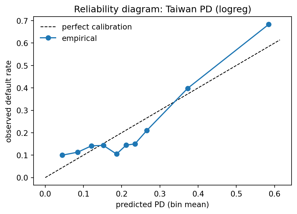
### Calibration under drift
Performance metrics are not the only thing to monitor. A well-calibrated scorecard has predicted PD equal to observed PD on every decile. Drift that does not change AUC can still destroy calibration.
```{python}
from sklearn.metrics import brier_score_loss

def reliability_table(y, p, n_bins=10):
    q = np.quantile(p, np.linspace(0, 1, n_bins + 1))
    q[0], q[-1] = -np.inf, np.inf
    rows = []
    for j in range(n_bins):
        m = (p >= q[j]) & (p < q[j+1])
        if m.sum() == 0:
            continue
        rows.append({'bin': j, 'n': int(m.sum()),
                     'pred': float(p[m].mean()),
                     'obs':  float(y[m].mean())})
    return pd.DataFrame(rows)

rel = reliability_table(te['default'].values, p_te, n_bins=10)
brier = brier_score_loss(te['default'].values, p_te)
print(rel.to_string(index=False))
print(f"Brier = {brier:.4f}")
```
```{python}
fig, ax = plt.subplots(figsize=(5.5, 4.0))
ax.plot([0, rel['pred'].max() * 1.05], [0, rel['pred'].max() * 1.05],
        'k--', lw=1, label='perfect calibration')
ax.plot(rel['pred'], rel['obs'], 'o-', lw=1.5, label='empirical')
ax.set_xlabel('predicted PD (bin mean)')
ax.set_ylabel('observed default rate')
ax.set_title('Reliability diagram: Taiwan PD (logreg)')
ax.legend(frameon=False)
fig.tight_layout()
plt.show()
```
The calibration table is the anchor artifact for the validator. An expected-vs-observed chi-square test against the table is the formal backtest, with degrees of freedom equal to the number of populated bins minus one.
### Performance under simulated concept drift
A laboratory for a monitoring pipeline is a controlled concept drift. We induce one by flipping the sign of the relationship between a single feature and the outcome in the test set, while keeping the feature distribution constant. The score stays on the same distribution; only the label-feature relationship moves.
```{python}
rng_c = np.random.default_rng(SEED + 1)
te_concept = te.copy()
# Induce concept drift: flip labels for a subset where a chosen feature is high
mask = te_concept['PAY_0'] >= 2
flip = rng_c.random(mask.sum()) < 0.5
y_concept = te_concept['default'].values.copy()
idx = np.where(mask)[0][flip]
y_concept[idx] = 1 - y_concept[idx]

auc_concept = roc_auc_score(y_concept, p_te)
psi_score_concept = psi_from_scratch(p_te, p_te)  # scores are unchanged
print(f"AUC pre-drift    = {auc:.4f}")
print(f"AUC post-concept = {auc_concept:.4f}")
print(f"PSI(score)       = {psi_score_concept:.4f}  (zero, scores unchanged)")
print(f"delta AUC        = {auc - auc_concept:.4f}")
```
The score distribution is unchanged, so PSI is zero. AUC drops sharply. Only an outcome-linked monitor catches this kind of drift; it is invisible to any feature- or score-distribution-only pipeline.
### DeLong vs bootstrap variance on the same data
For a paired champion-challenger comparison on the same test set, we can compare DeLong and bootstrap. The DeLong approach is cheaper but assumes asymptotic normality; the bootstrap is slower but distribution-free.
```{python}
from sklearn.ensemble import GradientBoostingClassifier
gb = GradientBoostingClassifier(n_estimators=50, max_depth=3, random_state=SEED)
gb.fit(tr[feat_cols].values, tr['default'].values)
p_te_gb = gb.predict_proba(te[feat_cols].values)[:, 1]
auc_gb = roc_auc_score(te['default'].values, p_te_gb)

lo_gb, hi_gb, _ = bootstrap_auc_ci(te['default'].values, p_te_gb, n_boot=400)
print(f"champion (logreg) AUC = {auc:.4f}  CI = [{lo:.4f}, {hi:.4f}]")
print(f"challenger (GB)   AUC = {auc_gb:.4f}  CI = [{lo_gb:.4f}, {hi_gb:.4f}]")

# Paired bootstrap of the delta
def paired_delta_ci(y, p1, p2, n_boot=400, alpha=0.05, seed=SEED):
    y = np.asarray(y); p1 = np.asarray(p1); p2 = np.asarray(p2)
    n = len(y); rng_b = np.random.default_rng(seed)
    deltas = np.empty(n_boot)
    for b in range(n_boot):
        idx = rng_b.integers(0, n, size=n)
        if y[idx].sum() in (0, n):
            deltas[b] = np.nan; continue
        deltas[b] = roc_auc_score(y[idx], p2[idx]) - roc_auc_score(y[idx], p1[idx])
    deltas = deltas[~np.isnan(deltas)]
    return float(np.quantile(deltas, alpha / 2)), float(np.quantile(deltas, 1 - alpha / 2))

lo_d, hi_d = paired_delta_ci(te['default'].values, p_te, p_te_gb)
print(f"delta AUC (challenger - champion) 95% CI = [{lo_d:.4f}, {hi_d:.4f}]")
```
If the paired delta interval excludes zero, the challenger is a statistically significant improvement. That is the quantitative half of the promotion gate. The qualitative half (calibration, fairness, stability, interpretability, operational fit) is what the validator adds.
## Scalability
### Polars for batch scoring
Pandas is not the right tool for a 100M-row scoring job. Polars is built on Arrow, uses a columnar execution engine, and runs multi-threaded by default. For a scorecard-style pipeline (numeric inputs, bounded feature count), the Polars code is nearly identical to pandas, and it ingests Parquet directly.
```{python}
import polars as pl

pl_df = pl.from_pandas(te[feat_cols].astype('float32'))
t0 = time.perf_counter()
X = pl_df.to_numpy()
p = pipe.predict_proba(X)[:, 1]
pl_out = pl_df.with_columns(pl.Series('pd', p))
print('polars batch score:', f"{(time.perf_counter()-t0)*1000:.1f} ms for {len(pl_out)} rows")
print(pl_out.select(['LIMIT_BAL', 'AGE', 'pd']).head(3))
```
For tree ensembles, the Polars pattern typically vectorizes feature extraction (lazy frame with expressions) and delegates the final `predict_proba` to the native backend (LightGBM's `predict`, XGBoost's `DMatrix`, CatBoost's `Pool`).
The pandas-to-Polars migration is not automatic. Three rough edges show up repeatedly in credit pipelines. First, Polars does not have a notion of row index; pandas idioms that use `.loc` with a multi-index need to be rewritten with group-by expressions. Second, Polars defaults to eager execution for `DataFrame` and lazy for `LazyFrame`; the performance win comes from the lazy API with its query optimizer, which requires rewriting the pipeline as chained expressions rather than mutations. Third, date/time handling differs: Polars uses microsecond precision natively, while many banking datasets use nanosecond or second precision, and implicit conversions can silently drop precision. The migration effort pays off: on the kind of join-and-aggregate workloads that dominate credit feature engineering, Polars typically runs 5 to 20 times faster than pandas on a single machine, with no Dask-style cluster coordination overhead.
### Dask for out-of-core scoring
When the scoring batch does not fit into RAM, Dask splits the frame into partitions and applies the model per partition. The pattern is a `map_partitions` over a Dask DataFrame.
```{python}
import dask.dataframe as dd

big = pd.concat([te[feat_cols]] * 3, ignore_index=True)
ddf = dd.from_pandas(big, npartitions=4)

def score_part(pdf):
    p = pipe.predict_proba(pdf.values.astype('float32'))[:, 1]
    return pdf.assign(pd=p)

meta = {c: 'f4' for c in feat_cols}; meta['pd'] = 'f8'
scored = ddf.map_partitions(score_part, meta=meta).compute()
print('dask scored rows:', len(scored), '  head:', scored['pd'].head(2).tolist())
```
The memory argument matters in credit: a full portfolio re-score at Basel IRB capital cadence can involve tens of millions of exposures, joined against their collateral and LGD models. Dask composes with Polars (via `dask.dataframe` on Arrow) and with cluster managers (Kubernetes, YARN, Coiled).
A practical note on partition sizing: Dask's default partition size is 128 MB, which is usually too large for model scoring because the model holds its own memory footprint and the prediction operation is CPU-bound. Partitions of 25 to 50 MB tend to give better parallelism on 8 to 16 core machines. The scheduler output (available via `scored.dask` or the Dask dashboard) shows the critical path; any single partition that dominates wall-clock time is the one to split further.
Spark is the enterprise-scale alternative to Dask. For credit-rating workloads at IRB capital scale (hundreds of millions of exposures), Spark with a Pandas UDF is the standard pattern. The Pandas UDF lets each executor materialize a partition as a pandas DataFrame, apply the model, and return a pandas Series; the serialization cost is paid once per partition. A typical Spark deployment will run the training in a single-node environment (because hyperparameter search dominates) and reserve the cluster for inference and feature engineering. That asymmetry (train on one node, score on many) is the opposite of many ML framework defaults, and the MLOps pipeline has to accommodate both.
### Kafka streaming (conceptual)
For real-time adjudication, the production pattern is:
1. A Kafka topic receives application events.
2. A stream processor (Flink, Spark Structured Streaming, or a Python consumer backed by `aiokafka`) pulls events, calls the model, and writes the score to an outbound topic.
3. Downstream consumers (decision engine, SIEM, fraud monitor) subscribe to the scored topic.
The model itself runs behind a sidecar service, not embedded in the stream processor, so the model lifecycle is independent of the stream-processing topology. The sidecar is what MLflow or Seldon Core or KServe ships as an image. Drift detection is another stream job: it windows the scored topic by tumbling intervals (one hour or one day), computes PSI, and emits an alert topic.
There are three reasons this separation matters in credit. First, the stream processor's release cadence is dictated by the team that owns the topology (often a data-platform team), not by the model team; a pickled model in a Flink job means every model release is a Flink release. Second, Kafka's exactly-once semantics apply to the topology; the model sidecar makes decisions based on message payload, so it does not need to be exactly-once as long as the downstream consumer idempotently handles duplicates. Third, the sidecar is the object the model risk team audits; embedding the model in a Flink operator hides the inference path from the audit trail.
A concrete streaming architecture for a consumer-lending decision pipeline: Kafka topic `applications` receives ingress events. A Flink job enriches each event with features from the feature store (using async I/O to avoid blocking). The enriched event is written to `applications_enriched`. A Python consumer (or a KServe model deployment subscribed via a Kafka source) reads `applications_enriched`, calls the model sidecar, and writes the scored event to `applications_scored`. A decision engine reads `applications_scored`, applies policy rules, and writes `decisions`. The drift monitor reads `applications_scored` on a tumbling window, computes PSI against a rolling reference (stored in Redis), and emits to `drift_alerts`. Each topic is its own audit trail; the combined log is the immutable record of every decision the bank made.
### Ray Serve
@moritz2018ray introduced Ray as a general distributed framework; Ray Serve is its serving layer. Ray Serve handles fractional GPUs, request batching, and replica autoscaling with a Python-native API. For credit, the important property is deterministic batching: incoming requests up to a timeout window are grouped into a batch and scored together, which pushes GPU utilization up without violating the per-request latency SLO. The skeleton looks like this (not run to keep the chapter deterministic):
```python
# Conceptual only, not executed in this chapter
# from ray import serve
# @serve.deployment(num_replicas=2, ray_actor_options={'num_cpus': 2})
# class PDModel:
#     def __init__(self, model_uri):
#         self.sess = rt.InferenceSession(model_uri, providers=['CPUExecutionProvider'])
#     @serve.batch(max_batch_size=64, batch_wait_timeout_s=0.01)
#     async def __call__(self, requests):
#         X = np.stack([r.features for r in requests]).astype('float32')
#         return self.sess.run(None, {'X': X})[1][:, 1].tolist()
```
### Horizontal scaling: replicas, autoscaling, and cold starts
A single serving replica handles a bounded request rate. Horizontal scaling adds replicas; autoscaling adjusts the replica count based on load. The two autoscaling metrics that matter for credit are request rate per replica and request-queue depth. CPU-based autoscaling is a lagging indicator (CPU utilization spikes after the queue builds), and it often triggers false scaling events on batched inference. The recommended pattern is to autoscale on queue depth (or equivalent: in-flight request count), with a target that leaves 20 to 30 percent headroom.
Cold starts are the reason many credit platforms keep a minimum replica count above zero. A fresh Python container with a 500 MB ONNX model plus onnxruntime plus FastAPI takes 5 to 15 seconds to become ready. During that window, incoming traffic is either queued or load-balanced to an existing replica, which can overload the existing replica and cause cascading failures. Knative can scale to zero, but for a credit origination channel with a 99.9 percent availability SLO, scaling to zero is usually a false economy. A minimum of two replicas (for redundancy) and an autoscaler that pre-warms a new replica at 70 percent load (before full saturation) is the typical tuning.
### Cost of inference
A rough unit-economics table for online credit scoring on commodity cloud hardware (roughly 2 vCPU and 4 GB container, on-demand pricing as of 2024):
| Backend | p99 latency (single row) | Throughput (1 replica) | Approx cost per 1M scores |
|---|---|---|---|
| sklearn + FastAPI + uvicorn | 5-15 ms | 300-1000 rps | 0.05-0.20 USD |
| ONNX Runtime + FastAPI | 1-5 ms | 2000-8000 rps | 0.01-0.05 USD |
| ONNX Runtime + Rust or Go server | 0.3-1 ms | 10k-50k rps | below 0.01 USD |
| LightGBM or XGBoost + FastAPI | 2-8 ms | 1500-5000 rps | 0.02-0.08 USD |
| Neural (PyTorch + TorchServe, CPU) | 10-50 ms | 100-500 rps | 0.20-1.00 USD |
| Neural (GPU, batched Ray Serve) | 5-20 ms | 5k-20k rps | 0.05-0.20 USD |
The cost column is a rule of thumb. It ignores data egress, authentication, and the model-governance overhead. Credit-specific workloads should also add a per-inference cost for feature retrieval (usually a feature-store lookup of 1-3 ms).
## Deployment
### The deployment architecture in one picture
A credit-scoring service in a mature shop sits at the intersection of five systems: the feature store (online and offline read paths), the model registry (the artifact source), the serving platform (the compute), the monitoring pipeline (the feedback loop), and the decision engine (the policy layer downstream). Every request traverses all five. The ingress comes from the origination channel (web form, mobile app, branch terminal, broker API). The request ID is generated at ingress, propagated through every layer, and is the join key for all downstream logs. The feature store enriches the request with cached or computed features. The model service scores. The decision engine applies policy. The response goes back to the channel. Every layer writes to the log. The monitoring pipeline reads from the log on a windowed schedule.
This architecture has two design properties that matter for credit. First, the model service is stateless with respect to the decision; it does not know what policy will be applied. That separation keeps the model's behavior auditable (the score is the score, independent of whether the policy is aggressive or conservative today). Second, the decision engine is the one layer that sees the full context (score, policy, channel, applicant history) and therefore is the one layer that can enforce invariants ("no decline without a reason code," "no approval above the capital limit," "human review for any score within 5 points of the cutoff").
### Cloud-agnostic managed services
Three managed ML services cover the vast majority of cloud-deployed credit models. AWS SageMaker Inference Endpoints package a container into a scalable HTTPS endpoint, with SageMaker Model Registry providing the lineage. GCP Vertex AI Online Prediction does the same with Vertex Model Registry and autoscaling. Azure ML Online Endpoints wrap the model into an "online deployment" behind an endpoint with traffic splitting. All three support either pre-built inference containers (which consume an MLflow pyfunc or a scikit-learn pickle) or bring-your-own-container. For credit-scoring shops, the deciding factor is rarely performance. It is whether the control plane integrates with the bank's IAM, VPC, and KMS setup.
SageMaker's specific features for credit include the shadow-variant capability (a built-in ability to deploy a challenger behind the same endpoint and split traffic), model-monitor jobs (pre-built PSI-like drift detection that runs on scheduled batches against a baseline), and the SageMaker Clarify bias-detection tooling. The practical caveat is that SageMaker's Model Monitor defaults to a simpler drift metric than a credit validator typically needs; most shops either configure it carefully or bypass it in favor of a custom monitoring pipeline that produces artifacts the validator trusts.
Vertex AI's equivalent is the Model Monitoring service, which supports skew and drift detection at configurable thresholds. Vertex's advantage is the tight integration with BigQuery for outcome linkage: the scored records can be written directly to a BigQuery table, joined to outcome tables at maturity, and analyzed with SQL. This matters because the credit validator's preferred working language is SQL, not Python.
Azure ML Online Endpoints integrate with Azure Monitor and Application Insights, and they support a managed online deployment and a Kubernetes online deployment (AKS-backed). The Kubernetes backend is the common choice for banks that already run AKS clusters and want a single operational plane. Azure's model-data-collector writes request and response pairs to a Blob Storage account, which is then the source for drift monitoring.
### Kubernetes with Knative
For teams that prefer an open stack, the canonical pattern is Kubernetes with a serving CRD (Knative Serving, KServe, or Seldon Core). The deployment lives as a YAML manifest in the model repository, gets rendered by a CI job, and is applied via GitOps (ArgoCD or Flux). Knative autoscaling can scale a deployment to zero replicas, which is attractive for rarely-used models in the inventory. The resulting deployment object is part of the model's audit trail, which simplifies SR 11-7 documentation.
KServe is the evolution of KFServing and is the closest open-source equivalent to SageMaker's managed endpoints. It adds model-specific features: transformer pre- and post-processing containers, a standard inference protocol (V1 and V2), and integration with explainers (Alibi) and outlier detectors (Alibi Detect). For credit, the attractive feature is V2's built-in batching and its support for canary releases at the CRD level: one YAML specifies both versions and the traffic split. The monitoring integration is native: Prometheus scrapes request counts, latencies, and error rates, and a Grafana dashboard shows them per model version.
Seldon Core takes a different design: the InferenceGraph is a DAG of inference components (model, transformer, combiner, router). For credit, a typical graph is transformer → ensemble-router → {champion-model, challenger-model} → combiner. The router sends traffic to the champion by default and mirrors a configurable fraction to the challenger. This is the shadow-traffic pattern implemented at the CRD layer, which means the infrastructure team does not have to touch the model code to reconfigure shadow.
The GitOps story matters for regulated shops. Every deployment is a commit. Every commit is signed. The set of signatures on the commit is the approval record; the main branch protection rule enforces that no deployment happens without the required signatures (model owner, validator, release engineer). When the regulator asks who approved the current production model, the git log of the `deployments/` directory is the answer.
### Dockerfile (multi-stage, non-root)
The container is the atomic unit of deployment. A model's Dockerfile should be multi-stage (to keep the runtime image small) and should run as a non-root user (hardening for regulated environments). Pin the base image by digest, not tag, so the build is byte-reproducible.
```
# Build stage
FROM python:3.11-slim AS build
WORKDIR /app
RUN apt-get update \
 && apt-get install -y --no-install-recommends build-essential \
 && rm -rf /var/lib/apt/lists/*
COPY requirements.txt .
RUN pip install --prefix=/install --no-cache-dir -r requirements.txt

# Runtime stage
FROM python:3.11-slim
RUN useradd --create-home --shell /bin/bash app
COPY --from=build /install /usr/local
WORKDIR /home/app
COPY --chown=app:app model.onnx app.py ./
USER app
EXPOSE 8080
HEALTHCHECK --interval=10s --timeout=3s \
  CMD curl -fsS http://localhost:8080/health || exit 1
CMD ["uvicorn", "app:app", "--host", "0.0.0.0", "--port", "8080", "--workers", "2"]
```
Three rules follow. The production image contains only runtime dependencies. The build tools never ship. The user is unprivileged. The healthcheck matches the FastAPI endpoint the Kubernetes probe will hit.
### Blue/green, canary, and shadow
Release strategies are what convert a container image into live traffic. The three patterns that matter for credit:
**Blue/green.** Two identical environments. Traffic swings from blue to green atomically. Rollback is a reverse swing. Blue/green is simple but coarse: the first request after the swing hits the new model with 100 percent of the traffic, so any regression is fully exposed.
**Canary.** A small fraction (1 percent, 5 percent, 10 percent) of traffic hits the new model. Metrics (AUC on labeled outcomes, PSI on scores, error rate) are monitored in real time. If they pass a threshold, the canary is promoted. This is the dominant pattern in large consumer-credit shops because it bounds the blast radius of a bad release to the canary fraction.
**Shadow (dark launch).** 100 percent of traffic hits both models. Only the champion's prediction is served to the caller. The challenger's prediction is logged for offline comparison. Shadow is the most information-rich of the three, because every request is a paired observation with the same features and the same downstream outcome. The cost is double the compute. Shadow mode is how champion-challenger campaigns are run for credit scorecards in regulated environments, because it produces a paired sample without exposing any applicant to the challenger's decisions.
Champion-challenger is itself a formal discipline. The champion is the production model. One or more challengers are scored in shadow for a prescribed campaign length (often 90 days or one full performance window). A hypothesis test (usually a DeLong test on AUC, a calibration chi-square, and a business-KPI comparison) decides whether a challenger is promoted. The entire campaign is documented and reviewed by model risk management before the swap happens. SR 11-7's "effective challenge" language is interpreted by most US banks as a requirement that every material model has a live challenger somewhere in the monitoring pipeline.
### Progressive delivery patterns in detail
Canary promotion is usually organized as a sequence of fixed traffic steps: 1 percent for an hour, then 5 percent for a day, then 25 percent for a week, then 100 percent. The step durations align with the statistical power needed at each level. At 1 percent of a 100k-application-per-day pipeline, 1000 canary predictions per day support detection of a 0.5 percentage point shift in approval rate with about 80 percent power at alpha 0.05. That is sufficient to catch a catastrophic regression. A 5 percent step supports detection of a 0.2 percentage point shift. A 25 percent step supports the detection of subtle bias and fairness regressions. The mathematical design of the promotion gate is the operational translation of statistical power analysis into a release calendar.
Rollback is a first-class operation. A canary that fails any gate is immediately reverted by pointing the alias back to the prior version. The revert should complete in under 60 seconds, because the blast radius of a bad release is cumulative in time. A 10-minute revert at 25 percent traffic on a 100k-per-day pipeline exposes roughly 1700 applicants to the bad model. The operational cost of a slow revert, compared to a fast one, is the difference in applicant-count times the average loss per misdecision.
Feature flags are the finer-grained complement to canaries. A feature flag toggles a specific code path (for example, a new feature in the preprocessing pipeline) without deploying a new model. Flags are evaluated per request, per session, or per cohort, with a configuration service (LaunchDarkly, Unleash, or a self-hosted Postgres-backed system) holding the state. For credit, flags are the mechanism for A/B tests on policy rules (cut-off thresholds, risk-based pricing tiers) that interact with the model output. The flag service itself is a model consumer and must be included in the monitoring pipeline.
### Shadow-traffic logging and replay
Shadow logging captures the challenger's prediction for every request the champion handled. The logged record must include the full feature vector, the champion score, the challenger score, a timestamp, and a stable identifier that links back to the downstream outcome. The storage backend (S3 + Parquet, Delta Lake, or BigQuery) must support point-in-time queries. The replay tooling reads the shadow log and recomputes the challenger's predictions offline against a new challenger version, so that a challenger can be tested without new shadow traffic. Replay is how a shop iterates on challengers between deployments.
The shadow log also provides the basis for the fairness audit. For every decline the champion issued, the shadow log has the challenger's alternative score. A model risk analyst can ask: if we had deployed the challenger, how many additional approvals would we have given, and in what demographic distribution? That question is the operational heart of fair lending analysis, and it is answerable only because the shadow log preserves the counterfactual.
### Monitoring stack
The monitoring stack should observe the model, not just the process. At minimum:
1. Request logs (request ID, features hash, score, latency, model version).
2. Score distribution rollups (hourly or daily PSI against a reference window).
3. Feature distribution rollups (CSI per feature, for the top features by importance).
4. Outcome-linked performance (AUC, KS, calibration) computed weekly or monthly, with bootstrap CIs.
5. Drift alerts, Page-Hinkley on aggregate approval rate and on selected segments.
6. Business KPIs: approval rate, cut-off distribution, loss curves by vintage.
Alerting rules must themselves be governed. A monitor with an unmanaged false-positive rate is not a control, it is a paging habit. Document the alert thresholds (PSI above 0.25 is typical, Page-Hinkley lambda calibrated to give an expected false-alarm interval of 30 days under $H_0$), the escalation path, and the rollback procedure, in the same document that covers the model itself.
### Observability stack
A concrete observability stack for a credit model in production has four layers. The **application layer** runs inside the serving container: structured logs (JSON), request/response payload samples (with PII redaction), request IDs, and exception traces. Log shipping (Fluent Bit, Vector, or Logstash) feeds the logs to a central store (Elasticsearch, Loki, or Splunk).
The **metrics layer** exposes Prometheus metrics from the serving container: request count, request duration histogram, error count, and model-specific counters (prediction distribution buckets, feature-value distribution samples). Grafana dashboards plot the metrics per model version, per canary cohort, and per time window.
The **feature layer** logs a random sample of request features to a feature log (BigQuery, Snowflake, Delta Lake), with retention matched to the monitoring window. The feature log is the source for PSI and CSI computation, typically as a scheduled Airflow or Dagster job.
The **outcome layer** joins the logged predictions to realized outcomes (delinquency, write-off, recovery) as they arrive, with the join key being the stable application identifier. The outcome layer is what feeds the backtest: the realized bad-rate in each decile, the realized KS, the realized Gini. Because the outcome layer has a lag (90 days minimum for early delinquency), it is the slowest feedback loop in the system; every other monitor is a proxy for it.
### Alert hierarchy
A mature monitoring pipeline has a three-level alert hierarchy. **P0 alerts** are immediate-page: a model is down, error rate is above 1 percent, latency p99 is above 500 ms, or the deployment is returning stale predictions. P0 alerts go to the on-call engineer via PagerDuty or equivalent.
**P1 alerts** are next-business-day investigation: PSI above 0.25 on the score, CSI above 0.25 on a top-5 feature, AUC outside the bootstrap confidence interval for two consecutive weeks, approval rate shift above 2 percentage points week-over-week. P1 alerts go to the model owner and the model validator.
**P2 alerts** are included in the weekly or monthly model risk report: any PSI between 0.10 and 0.25, any slow-trending AUC drift, any concentration shift in a cohort. P2 alerts do not interrupt work; they are summarized and reviewed by the model risk committee at its standing cadence.
Separating the three prevents alert fatigue. A system that pages the on-call for every CSI excursion becomes a system the on-call ignores. Regulators understand this; the SR 11-7 commentary on "effective" monitoring implicitly requires an alert regime that is actually actionable.
## Regulatory considerations
### SR 11-7 (Federal Reserve) and OCC 2011-12
SR 11-7 is the foundational US supervisory letter on model risk management [@fed2011sr117]. OCC 2011-12 is the materially identical guidance for national banks [@occ2011handbook]. Both require three interlocking disciplines:
1. **Model development.** Every model has documented purpose, theoretical soundness, data lineage, assumptions, and limitations. This is the model documentation, owned by the model developer.
2. **Model validation.** Independent validation reviews conceptual soundness, outcomes analysis (backtesting against realized outcomes), and ongoing monitoring. The validator is organizationally independent of the developer.
3. **Governance, policies, controls.** A model inventory, a model risk policy, a model risk committee, and annual attestations.
MLOps maps directly onto these three disciplines. The experiment-tracking server is the developer's artifact. The monitoring dashboard and backtest reports are the validator's artifact. The model registry is the inventory. The CI/CD pipeline (with required approvals, branch protection, and signed commits) is the control.
The practical implication: the model registry must be able to answer, for any model in the inventory, seven questions with an audit trail. Who developed it. Who validated it. What version is live. When was it last backtested. What drift has been observed. What incidents have been logged. What is the rollback plan. A registry that stores only the artifact and the metrics is not enough.
#### Model tiering and the materiality principle
SR 11-7 does not require the same level of scrutiny for every model. Institutions assign a **tier** (usually Tier 1 through Tier 4) based on materiality, which is typically a function of the financial impact, the reputational impact, and the regulatory impact of the model failing. Tier 1 models (the institution's primary PD scorecards, the capital-IRB models, the major stress-test models) get the full treatment: annual validation, quarterly monitoring, documented challengers, formal change control. Tier 4 models (internal-use ranking models, marketing propensity scores with no direct customer impact) get a lighter regime: biennial review, periodic monitoring, informal change management.
The tiering exercise itself is a governance artifact. It is reviewed annually by the model risk committee, and a model's tier can change based on its expanding use (a Tier 4 propensity score that gets integrated into an automated decision engine becomes Tier 2 or higher). MLOps tooling supports tiering by enforcing the cadence: a model registry tagged Tier 1 cannot be deployed without a current validation signature, while a Tier 4 model can be deployed with a lighter gate.
#### Effective challenge in practice
The phrase "effective challenge" appears in SR 11-7 multiple times. It is the requirement that the model be subject to critical analysis by objective, informed parties who identify model weaknesses. In practice, effective challenge has three operational forms. First, **pre-deployment challenge**: the validation team runs its own benchmark model (typically a simpler or alternative-algorithm model) and compares against the proposed champion. If the challenger is within 1 to 2 percent AUC of the champion, the validator asks why the more complex model is justified. Second, **live challenge**: a challenger runs in shadow in production, as described above. Third, **periodic challenge**: at each annual review, the model owner and validator re-examine whether the model's assumptions still hold, whether new data sources have become available, and whether an alternative framework would now be preferred.
Effective challenge is expensive. It is also the single requirement most commonly failed in supervisory exams. The MLOps infrastructure that makes it cheap (a shadow-logging pipeline, a replay harness, a validation benchmark suite in CI) is the same infrastructure that makes the institution defensible on inspection.
### PRA SS1/23
The Bank of England's Supervisory Statement SS1/23 [@pra2023ss123] is the UK counterpart, effective May 2024, and it is materially broader than SR 11-7. It covers not just credit models but any model used in a material decision, including stress-testing, capital, liquidity, and operational resilience. Its five principles are (1) model identification and inventory, (2) governance, (3) development, implementation and use, (4) independent validation, and (5) model risk mitigation. The principle most often underappreciated is the fifth: every material model must have compensating controls (human override, limits, alternative models) that remain effective when the model misfires.
### EU AI Act
The EU AI Act [@eu2024aiact] classifies credit-scoring systems for natural persons as high-risk (Annex III, point 5(b)). High-risk systems have obligations across design, testing, documentation, human oversight, accuracy, robustness, cybersecurity, and post-market monitoring. Article 72 requires a post-market monitoring system that is proportionate to the nature of the AI system and the risks it poses. For a credit scorecard, that means drift detection, performance monitoring, and incident reporting, with a documented plan reviewed annually. The enforcement date for high-risk AI systems is 2 August 2026, with earlier dates for prohibited systems and general-purpose AI models.
The interaction between Article 22 GDPR (the right not to be subject to a decision based solely on automated processing that produces legal effects) and the AI Act is the live regulatory question for European credit lenders. Most banks address Article 22 by documenting a meaningful human review pathway (typically for borderline and declined applications), and by providing the applicant with the logic involved, the significance, and the envisaged consequences of the decision [@eu2016gdpr].
Post-market monitoring under Article 72 is operationalized as a **post-market monitoring plan**, submitted to the relevant conformity-assessment body (or documented internally for systems that use self-assessment). The plan specifies the metrics monitored, the thresholds, the reporting cadence to the competent authority, and the incident-reporting process. The AI Act also introduces Article 73, which requires notification to the authority of "serious incidents" within 15 days (or less for incidents involving harm to life or health). For a credit scorecard, a serious incident is defined by the deployer's risk management system, but the default interpretation is any unresolved drift that persists for more than a quarter, any systematic bias discovered in post-hoc analysis, or any infringement of Union law attributable to the model.
The AI Act's technical documentation requirements (Annex IV) extend the SR 11-7-style documentation pack with several additional items: a description of the intended purpose, the persons on whom the system is intended to be used, the known or foreseeable circumstances that may lead to risks to health and safety or fundamental rights, the human-oversight measures built in, the input data specifications, the expected lifetime of the system, the cybersecurity measures, and the metrics used to measure performance in the post-market phase. Each of these maps to an MLOps artifact: the model card, the monitoring dashboard, the penetration test report, the threat model, and so on.
### Basel backtesting and validation cadence
Basel II's use test and the Basel Committee's validation working paper [@bcbs2005validation] define the statistical expectations for IRB models. Three cadence anchors matter:
1. **Annual validation.** At minimum, every IRB PD, LGD, and EAD model must be validated annually. Validation covers discriminatory power (AUC, Gini, KS), calibration (Hosmer-Lemeshow or equivalent chi-square), and stability (PSI).
2. **Ongoing monitoring.** Between annual validations, the institution must monitor performance. The EBA GL/2017/16 [@eba2017glom] specifies for PD models a migration-matrix check, calibration by grade, and stability of the rating philosophy.
3. **Triggered revalidation.** A material drift (PSI above 0.25 at score level, or a structural break in approval rates, or a failed calibration test) triggers an out-of-cycle revalidation. The trigger criteria must be predefined and documented.
### Fair lending and disparate impact monitoring
Every US credit model is subject to ECOA Regulation B, which prohibits discrimination on prohibited bases (race, color, religion, national origin, sex, marital status, age, receipt of public assistance). Compliance has two prongs. Disparate treatment is the use of a prohibited basis as an input; the MLOps pipeline enforces this by having an explicit allow-list of features, with prohibited bases kept out of the training set. Disparate impact is a materially different outcome across protected classes even when the model does not use the prohibited basis; this requires a monitoring step.
The standard disparate-impact test uses the Bayesian Improved Surname Geocoding (BISG) method to probabilistically infer race from applicant surname and geographic data, runs the model over the inferred-race cohorts, and compares approval rates and error rates across cohorts. The 80 percent rule (approval rate for a protected class must be at least 80 percent of the approval rate for the majority class) is the traditional regulatory threshold; the statistical equivalent is a chi-square test on the contingency table of decision and cohort, with a Bonferroni correction across the protected-class set. The MLOps pipeline runs the BISG inference and the disparate-impact calculation as a scheduled job (typically monthly), writes the output to a fair-lending dashboard, and alerts the fair-lending officer on any material regression.
The monitoring pipeline does not stop at approval rates. The 2022 CFPB Special Edition of Supervisory Highlights emphasized that fair-lending analysis should cover pricing, limit assignment, and adverse action reason code distribution, not just approval. For a scorecard, the pipeline therefore produces four fairness metrics per cohort per time window: approval rate, approved-APR distribution, assigned-limit distribution, and reason-code distribution. Each has its own alert threshold; each has its own escalation path to the fair-lending officer.
### Documentation checklist
A minimum documentation pack for a deployed credit model contains:
- The model card: purpose, intended population, exclusions.
- The development document: theoretical basis, data lineage, feature engineering, training protocol, hyperparameters, validation results.
- The validation report: independent replication, backtest, stress test, conceptual soundness review.
- The monitoring plan: metrics, thresholds, cadence, escalation, rollback.
- The deployment artifact: container digest, signature, ONNX digest, registry URI.
- The runbook: how to roll back, how to re-score a batch, how to trigger the human-review pathway.
- The incident log: every alert, every action.
Every item in the pack is versioned and linked from the model registry entry.
#### Lineage and reproducibility
Model lineage is the full chain of provenance from raw data to deployed artifact. In a well-designed pipeline the lineage is captured automatically: every MLflow run stores the git SHA, the data snapshot identifier, and the environment spec. Every registered model version links back to its run. Every deployment links to its registered model version. The chain is queryable: from a decision log entry, the auditor can traverse back through the deployment record, the registered model version, the training run, the data snapshot, and the git commit, all the way to the code and the raw data. That traversal is what SR 11-7 means by "comprehensive model inventory." It is not achievable by documentation alone; it requires tooling that enforces the links at creation time.
Data lineage is the other half of the problem. Feature pipelines often aggregate data from a dozen sources (core banking, payment processor, credit bureau, customer-relationship-management system, open-banking API). Each source has its own refresh cadence, its own schema evolution, and its own data-quality process. A feature catalog (DataHub, Amundsen, Unity Catalog) tracks the lineage at the column level: for each feature used by the model, the catalog records the source tables, the transformation code, the refresh schedule, and the data-quality checks. The catalog is the data-side mirror of the model registry, and the two should be cross-referenced.
#### Change management
Every change to a production credit model triggers a change-management process. The change-management ticket captures the motivation, the scope, the risk assessment, the validation plan, the rollback plan, the communication plan, and the approval signatures. The MLOps pipeline integrates with the ticketing system (ServiceNow, Jira Service Management, or a custom system): the CI job that promotes a model version to the production alias requires a valid ticket reference, and the ticket auto-updates as the deployment progresses. This integration is not optional; it is how a validator reconstructs, six months after the fact, what changed and why.
The taxonomy of changes matters. Minor changes (a retrain on the same features with the same hyperparameters, on updated data) can follow a lighter path. Major changes (a feature addition, a hyperparameter change, an architecture change) require full validation. Material changes (a change in the target definition, a change in the treatment population, a redesign of the decision threshold) may require regulator notification in IRB-permitted institutions. The MLOps pipeline tags each change with its category at commit time, and the CI gates enforce the category-specific requirements.
### Security posture
Credit-scoring services are attractive targets. The attack surface includes model-extraction attacks (adversaries probe the endpoint to reconstruct the scoring function), membership-inference attacks (adversaries determine whether a specific individual was in the training set, with PII implications), and adversarial-example attacks (adversaries craft feature vectors that produce desired scores). The MLOps response has four layers. First, strong authentication and rate limiting at the API gateway prevent extraction by volume. Second, differential-privacy or output-quantization at the model layer bounds the leakage per query. Third, the audit log flags anomalous query patterns (unusual feature distributions, repeated queries on similar inputs). Fourth, a red-team program routinely attempts the standard attacks and reports findings to the model risk team.
For regulated lenders, the relevant frameworks are NIST 800-53 (US federal), ISO 27001 (international), SOC 2 Type II (for service providers), and the emerging NIST AI Risk Management Framework. The AI Act's Article 15 requires high-risk AI systems to be "designed and developed in such a way that they achieve an appropriate level of accuracy, robustness and cybersecurity." Robustness in this context specifically includes resilience against adversarial examples and against the errors introduced by drift or degradation.
Secret management is the unglamorous but essential part. The model container should never embed credentials in its image layers. Database connection strings, API keys for the feature store, and signing keys for the outbound webhooks must be injected at runtime from a secret manager (HashiCorp Vault, AWS Secrets Manager, GCP Secret Manager). The CI pipeline scans every commit for accidentally committed secrets; any detection blocks the merge.
### Disaster recovery and business continuity
A credit-scoring service is a critical path for a lender; an extended outage stops origination and triggers contractual and reputational penalties. The disaster-recovery plan covers three failure modes. A **service-level outage** (the model container crashes) is handled by autoscaling and health-check-driven recovery; recovery time objective (RTO) is seconds. A **regional outage** (the cloud region is unavailable) is handled by multi-region deployment with traffic failover; RTO is minutes. A **model-level regression** (the deployed model produces materially wrong scores, discovered post-deployment) is handled by the rollback procedure; RTO is the time-to-detect plus the time-to-revert, typically minutes to hours.
The business-continuity plan covers the case where the model is unavailable for an extended period. For many lenders, the fallback is a simpler scorecard (a logistic regression on a reduced feature set, or a bureau-score-only rule) that can operate with degraded feature availability. The fallback model is itself versioned, validated, and monitored, and it is exercised quarterly to ensure it remains deployable. Treating the fallback as a second-class citizen is a common mistake; regulators specifically ask about the fallback in examinations.
### GDPR Article 22
Article 22 is narrower than many practitioners assume. It bars decisions based solely on automated processing that have legal or similarly significant effects, with three carve-outs: contractual necessity, explicit consent, and authorization by Union or Member State law. Credit decisions typically rely on the first or third. The safeguards required even under the carve-outs are three: the right to obtain human intervention, the right to express the applicant's point of view, and the right to contest the decision. In practice, banks operationalize Article 22 by building a review queue for declines, staffed by credit officers with override authority, and by logging every override with a justification that is itself auditable.
The Article 22 right to explanation is a live question in European case law. The Schufa judgment of the Court of Justice of the European Union (C-634/21, December 2023) held that the computation of a credit score that is then used by a third party as the basis for a decision is itself automated decision-making within the meaning of Article 22, triggering the information and safeguard rights. The practical effect on credit bureaus and lenders is that the "logic involved" disclosure cannot be a black-box statement; it must include the main features that drove the score for the specific applicant. SHAP values, Integrated Gradients, or feature-importance snapshots per decision are the operational implementation of this requirement, and they must be logged at decision time because reconstructing them later is both expensive and statistically lossy.
### CCAR, DFAST, and stress-testing implications
US IHCs and G-SIBs subject to the Federal Reserve's Comprehensive Capital Analysis and Review (CCAR) and the Dodd-Frank Act Stress Test (DFAST) must submit projections of credit losses under supervisory scenarios. The PD models feed directly into the loss projection. The MLOps implication is that the PD model in production must be the same model that feeds the stress-test submission, or the differences must be documented and justified. Many banks maintain a "stress-test vintage" of each model, frozen at the submission date, to ensure auditability. The model registry's alias mechanism is the right place to store these vintages: a dedicated "ccar-2026-submission" alias points to the frozen artifact.
### Adverse action notices under ECOA and FCRA
In the US, adverse action notices (required by the Equal Credit Opportunity Act and the Fair Credit Reporting Act) must state the principal reasons for an adverse decision. For model-driven decisions, the principal reasons are typically derived from the top-ranked feature contributions to the score, subject to a "reason code" mapping that translates technical features into consumer-facing language. The MLOps implication is that the reason codes are themselves a model artifact: they must be versioned with the model, validated for accuracy (the code must reflect a real feature contribution), and regenerated whenever the feature set changes. A scorecard that ships a new version but keeps the old reason codes is generating false adverse action notices, which is an enforcement risk. The reason-code generator runs at decision time, stores its output in the decision log, and is reviewed by model risk management as part of the validation pack.
### Basel IRB: use test and experience requirement
Beyond the statistical validation cadence, Basel IRB imposes the **use test** and the **experience requirement**. The use test requires that the PD model actually be used in the credit decision, in pricing, in limit setting, and in capital calculation; a model that is only used for capital is not eligible for IRB treatment. The experience requirement requires at least three years of use of the internal ratings before the model can be used for regulatory capital, and longer periods for foundation and advanced IRB. Both requirements have MLOps implications: the decision log must prove the model's use, the feature inputs must be stable over the three-year window, and any major change to the model requires a re-starting of the experience clock. This is why IRB shops are conservative about model upgrades; the cost of resetting the clock can exceed the benefit of a better model.
## Putting the pieces together: a reference pipeline
To close, a concrete end-to-end pipeline that ties together everything in this chapter. The pipeline is implemented in a monorepo with the following top-level layout:
- `data/` : versioned data snapshots (DVC or Delta time travel).
- `features/` : feature-store definitions, feature SQL, feature tests.
- `models/` : training code, model definitions, validation notebooks.
- `serve/` : FastAPI application, Dockerfile, ONNX export logic.
- `deploy/` : Kubernetes manifests, Knative services, CI/CD pipelines.
- `monitor/` : drift detectors, PSI/CSI jobs, alert rules.
- `governance/` : model cards, validation reports, inventory entries.
The developer workflow: a pull request in `features/` triggers feature-store tests and PIT-correctness verification. A pull request in `models/` triggers training on a sampled snapshot, a full MLflow log, and an automated benchmark against the current champion. Merge to main promotes the run to the "pending-validation" alias. The validator reviews the MLflow run, approves via a signed commit in `governance/`, which triggers the promotion to "staging". A deployment pull request in `deploy/` applies the Kubernetes manifest, which rolls out the staging version at 1 percent canary. Metrics gates are evaluated automatically; if they pass, the canary progresses through the standard step sequence. The final promotion to "production" is a signed commit by the release engineer. Every transition is logged to the inventory.
This pipeline is what the regulatory asks are really testing: not any single piece, but the end-to-end evidence that a reader can reconstruct from the logs. The pipeline is the compliance posture. The rest is implementation detail.
## Vietnam and emerging markets
### Market context
Vietnam's MLOps posture is shaped by three intersecting policies. Decree 53/2022/ND-CP implements the 2018 Law on Cybersecurity and requires that certain classes of personal and financial data of Vietnamese users be stored within Vietnam, with specific onshore-presence requirements for foreign service providers [@vn_decree53_2022]. Circular 13/2018/TT-NHNN sets the internal-control and risk-management framework for commercial banks, including expectations for model inventories, independent validation, and board-level reporting [@sbv_circular13_2018]. The SBV digital transformation roadmap (Decision 810/QD-NHNN) pushes banks to operate digital channels at scale while complying with those controls [@sbv_digital_roadmap2021].
The domestic cloud market has grown to meet these constraints. Viettel IDC, VNG Cloud, and FPT Smart Cloud operate Tier III and Tier IV data centers inside Vietnam and offer managed Kubernetes, object storage, and GPU instances sufficient to host the serving stacks described in this chapter. Hyperscaler providers (AWS, Azure, Google) serve Vietnamese customers from Singapore and Hong Kong regions. The practical choice for a credit MLOps pipeline is therefore not a single-cloud decision but a two-tier decision: which workloads must sit onshore for compliance, and which can run offshore for cost or feature reasons [@bis_emde_cloud2022; @worldbank2023vn_digital].
Supervisory capacity is evolving. SBV inspections still center on traditional credit, market, and liquidity risk, with model-risk specialists embedded in larger joint-stock commercial banks rather than in the supervisor. That asymmetry is narrowing, and the ADB has funded technical assistance on fintech supervision that informs SBV practice [@adb_vietnam_fintech2022; @imf_vietnam_fsap2019].
### Application considerations
Three operational patterns recur in Vietnamese credit MLOps pilots. First, the training-serving skew problem has a local twist: training often happens on hyperscaler GPU in Singapore under a data-processing agreement that anonymizes or aggregates before export, while serving must run onshore. Preprocessing objects therefore cross a trust boundary and must be versioned, signed, and byte-for-byte reproducible on both sides. ONNX plus a signed container is the minimum-viable pattern; adding a cryptographic hash of the preprocessor blob to the model card is the current best practice.
Second, the model inventory under Circular 13/2018 has a prescribed set of fields that maps closely but not exactly onto the global model-risk playbook. Internal-control reporting lines flow to the board audit committee and the risk committee with quarterly cadence, and any material model change is expected to be pre-notified to SBV for systemically important banks. MLflow plus a Postgres-backed inventory is sufficient technology; the governance wrapper must include Vietnamese-language model cards, validator sign-off in Vietnamese, and a documented map from SR 11-7 or PRA SS1/23 artifacts to the Circular 13 reporting templates [@sbv_circular13_2018; @fed2011sr117; @pra2023ss123].
Third, monitoring must account for the SBV reporting cadence. PSI and CSI are computed daily or weekly in the MLOps platform; a rollup feeds the quarterly internal-control report. Drift alerts that never surface in the board report are not compliant evidence, even if they trigger on-call pages internally.
### Rationalization
Why accept the cost of the localization constraint. Three reasons. First, the regulatory risk of non-compliance is direct and material: SBV can restrict the product line of a bank whose internal-control reporting is judged inadequate, and the Ministry of Public Security enforces Decree 53 with administrative fines. Second, customer trust is a first-order competitive asset in a market where bureau coverage is incomplete and consumers rely on reputational signals; a serving stack hosted entirely onshore is a marketable commitment. Third, latency. A payment-time scoring decision served from an onshore Viettel or VNG region beats the round trip to Singapore by tens of milliseconds, which matters for point-of-sale BNPL and for mobile money flows [@worldbank2023vn_digital].
Against this, multi-cloud federation is a real architectural cost. The cost is absorbed most easily by banks with mature platform teams, and most painfully by fintechs that grew on hyperscaler templates and must re-platform to enter the sandbox. The arbitrage so far has been to keep model training on hyperscalers with privacy-preserving aggregation and to move only serving and feature retrieval onshore. That arbitrage is stable under current rules but could tighten if data-localization scope expands.
### Practical notes
Concrete lessons from the past three years of Vietnamese deployments. One, budget six to nine months for the first domestic-cloud serving stack; the bottleneck is not compute but identity, network, and cryptographic key management integration with the existing core banking stack. Two, insist on bilingual model cards from day one; translating at the end of a project is slower than writing in parallel. Three, treat Decree 53 scope as an evolving boundary: read each SBV circular update against the current serving footprint and plan a quarterly scope review. Four, align the MLOps inventory field set with the Circular 13 report fields; a one-to-one correspondence eliminates reconciliation work at audit time. Five, test ONNX numerical parity between the training GPU region and the onshore serving CPU region; small FP32 differences across vendors have caused reason-code drift in at least two Vietnamese pilots.
@tbl-vn-mlops-stack is the working reference stack that has emerged in Vietnamese banks through 2025.
| Layer | Offshore option | Onshore option | Notes |
|---|---|---|---|
| Training compute | AWS/GCP GPU | Viettel IDC GPU | Onshore for PII-inclusive training |
| Feature store | Feast on managed Postgres | Feast on VNG Postgres | Residency governs choice |
| Model registry | MLflow SaaS | Self-hosted MLflow on FPT Cloud | Registry must follow data |
| Serving | SageMaker/Vertex | ONNX + FastAPI on Kubernetes | Onshore is the default |
| Monitoring | Datadog | Prometheus + Grafana | Domestic SIEM integration |
: Two-tier reference MLOps stack under Vietnamese data-localization constraints. {#tbl-vn-mlops-stack}
## Takeaways
- Training-serving skew is the single largest operational risk in a credit-scoring production system, and it is eliminated by making preprocessing and inference a single versioned artifact.
- Drift detection is a hypothesis-testing problem. PSI, CSI, KS, Page-Hinkley, and Wasserstein each answer a different question, and a production monitor uses all of them in combination, not in isolation.
- ONNX plus a signed container is the current best default for serving. It gives numerical parity with the training stack, cross-language portability, and an auditable artifact.
- Release strategy is a regulatory artifact. Shadow traffic and champion-challenger campaigns are not only engineering patterns, they are how SR 11-7 "effective challenge" and EU AI Act post-market monitoring get operationalized.
- A model without a monitoring plan, a rollback procedure, and a documented incident history is not in compliance with SR 11-7, OCC 2011-12, PRA SS1/23, or the EU AI Act. The documentation pack is the deliverable; the code is the means.
## Further reading
- @sculley2015hidden on hidden technical debt (the founding MLOps paper).
- @breck2017mltest on the 28-point production readiness rubric.
- @polyzotis2018datamgmt on data-management lifecycle in production ML.
- @paleyes2022challenges for the industrial survey.
- @klaise2020monitoring on monitoring and explainability together.
- @amershi2019software on software-engineering practices for ML.
- @schelter2018automating on model management.
- @zaharia2018accelerating on the MLflow design.
- @moritz2018ray on the Ray distributed framework.
- @crankshaw2017clipper on low-latency prediction serving (Clipper).
- @gama2014survey_concept on concept drift adaptation.
- @rabanser2019failing on empirical drift-detection methods.
- @fed2011sr117 and @occ2011handbook on US model risk management guidance.
- @pra2023ss123 on UK supervisory expectations.
- @eu2024aiact and @eu2016gdpr on the EU AI Act and GDPR Article 22.