---
execute:
echo: true
eval: true
warning: false
cache: true
---
# Neural Networks and Deep Learning {#sec-ch14}
::: {.callout-note appearance="simple" icon="false"}
**Scope: both retail and corporate.** MLP, embedding-based, and tabular deep models. Worked examples are retail (UCI German, Taiwan); the chapter documents why deep nets typically lose to GBT on tabular credit data of either kind.
:::
## Overview {.unnumbered}
Neural networks arrived in credit scoring before they were ready. Papers in the mid-1990s trained feedforward nets on UCI-sized tables, reported small AUC gains over logistic regression, and reviewers drew strong conclusions from thin benchmarks [@west2000neural; @atiya2001bankruptcy]. The large benchmarks of the 2010s put the discipline back on firmer ground. @lessmann2015benchmarking compared forty-one classifiers across eight credit datasets and placed single-hidden-layer neural nets in the middle of the pack, beaten by gradient boosting and heterogeneous ensembles but essentially tied with random forests on a rank-sum test. A decade later, @grinsztajn2022why formalized the folk wisdom: tree-based models still dominate on typical tabular data, and deep learning wins only when the structure of the input (sequence, image, graph, text) lines up with a deep inductive bias that trees cannot match.
This chapter takes deep learning seriously anyway. First, because deep models are now the only realistic option for the three structured modalities that sit next to credit: transaction sequences (@sec-ch18), digital footprints (@sec-ch17), and free-text narratives (@sec-ch25). Second, because attention-based architectures such as FT-Transformer [@gorishniy2021revisiting] and TabNet [@arik2021tabnet] have closed a meaningful fraction of the gap to gradient boosting on tabular data, and deep tabular models are now the interpretability target for distilled post-hoc explainers in many shops. Third, because deep learning is the only way to build joint representations across text, structured features, and sequences inside one model; the modern credit stack is not single-modality any more.
A cautious framing is in order. Everything in this chapter can be replaced, on Taiwan default or Home Credit, by a five-line XGBoost call that runs in half a second and will very likely beat the neural net by a modest but real margin. The value of the chapter is not "deep learning is a better credit scorer" (it usually is not). The value is that you walk away able to train, regularize, serialize, and deploy a neural net for credit, know when the structure of your data actually warrants one, and understand the math well enough to read a referee's report.
## Motivation {#sec-ch14-nn}
Three forces pushed neural networks back into the credit toolbox. The first was the open-source PyTorch and TensorFlow ecosystems [@paszke2019pytorch], which removed the engineering tax that killed 1990s-era neural credit scorers at institutions without dedicated research groups. The second was the switch from handcrafted features to learned representations for two high-volume credit modalities: transaction streams [@babaev2022coles] and mortgage loan histories [@sadhwani2021deep]. Both lean on recurrent or transformer architectures that simply do not exist in a tree-based toolkit. The third was regulatory: supervisors have started to accept non-linear models, provided the institution delivers the SR 11-7 documentation stack (validation, monitoring, challenger, explainability, fairness) around them.
The core tension is small data. Credit portfolios are imbalanced (default rates of 2 to 10% in prime retail, 15 to 25% in subprime or card) and, after carve-outs for time-out-of-sample validation, training samples of 50,000 to 500,000 rows are common. Deep networks are notorious for overfitting below a million rows unless regularization is aggressive. The benchmarks in @grinsztajn2022why use 1,000 to 10,000 rows and conclude that tree models win; @gorishniy2021revisiting use comparable sizes and conclude that carefully tuned transformers tie trees. The difference is almost entirely regularization discipline.
The tension is sharper in emerging markets. A Vietnamese finance company may have 30,000 to 150,000 labeled defaults across a multi-year window, with CIC pulls that cover only a fraction of the exposures and with cross-channel drift driven by fast eKYC-enabled growth [@cic_vietnam2023; @sbv_circular16_2020]. That is well below the thin-sample floor at which an MLP stops memorizing and starts generalizing, and it is the regime where the choice of regularization (dropout rate, weight decay, early-stopping patience) matters more than architecture. The Vietnam section at the end of this chapter spells out the defaults that have held up under SBV-style review.
## Notation {.unnumbered}
Let $(x_i, y_i)_{i=1}^n$ denote the training set, with feature vector $x_i \in \mathbb{R}^p$ and label $y_i \in \{0, 1\}$ (1 = default). A feedforward network with $L$ layers defines a function $f_\theta: \mathbb{R}^p \to \mathbb{R}$ with parameters $\theta = (W^{(\ell)}, b^{(\ell)})_{\ell=1}^{L}$, where $W^{(\ell)} \in \mathbb{R}^{d_\ell \times d_{\ell-1}}$ and $b^{(\ell)} \in \mathbb{R}^{d_\ell}$. The activation at layer $\ell$ is $a^{(\ell)}$, the pre-activation is $z^{(\ell)}$, and $\sigma(\cdot)$ is a nonlinearity (tanh, ReLU, GELU). Probability of default is $\hat{p}_i = \mathrm{sigmoid}(f_\theta(x_i))$, and the binary cross-entropy loss is $\ell(\theta) = -\tfrac{1}{n}\sum_i [y_i \log \hat{p}_i + (1 - y_i) \log(1 - \hat{p}_i)]$.
```{python}
#| label: setup
import os
os.environ.setdefault("OMP_NUM_THREADS", "1")
os.environ.setdefault("KMP_DUPLICATE_LIB_OK", "TRUE")

import sys, time, warnings
sys.path.insert(0, "../code")
warnings.filterwarnings("ignore")

import numpy as np
import pandas as pd
import torch
import torch.nn as nn
from sklearn.preprocessing import StandardScaler
from sklearn.linear_model import LogisticRegression
from sklearn.metrics import roc_auc_score, brier_score_loss

from creditutils import (
    load_german_credit, load_taiwan_default,
    train_valid_test_split, ks_statistic, stable_sigmoid,
)

SEED = 0
np.random.seed(SEED)
torch.manual_seed(SEED)
torch.set_num_threads(1)
```
## MLP architecture
### Forward pass
A multilayer perceptron alternates affine maps with nonlinear activations. For a network with layer widths $d_0, d_1, \ldots, d_L$ (where $d_0 = p$ is the input dimension and $d_L = 1$ for binary classification),
$$
a^{(0)} = x, \qquad z^{(\ell)} = W^{(\ell)} a^{(\ell-1)} + b^{(\ell)}, \qquad a^{(\ell)} = \sigma(z^{(\ell)}), \quad \ell = 1, \ldots, L-1,
$$ {#eq-mlp-forward}
with the output layer linear in the logit scale: $f_\theta(x) = z^{(L)} = W^{(L)} a^{(L-1)} + b^{(L)}$. For binary classification the predicted probability is $\hat{p} = \sigma_{\mathrm{sig}}(f_\theta(x))$, where $\sigma_{\mathrm{sig}}(u) = 1/(1 + e^{-u})$.
The hidden nonlinearity is a design choice. The classical choice is $\tanh$, which maps to $(-1, 1)$ and is smooth. The modern default is ReLU, $\mathrm{ReLU}(u) = \max(0, u)$, which has two appealing properties: it does not saturate on the positive side, so gradients flow even for large pre-activations, and it is piecewise linear, which makes the forward pass and its Jacobian cheap. For tabular credit nets the practical difference between ReLU, GELU, and SiLU is within noise; the choice matters far less than width and regularization.
### Universal approximation
The universal approximation theorem says that a network with one hidden layer of sufficient width and any non-polynomial activation can approximate any continuous function on a compact set to arbitrary accuracy [@cybenko1989approximation; @hornik1989multilayer]. Formally, if $\sigma$ is continuous, nonconstant, bounded, and non-polynomial, then for every $\varepsilon > 0$ and every continuous $g: [0, 1]^p \to \mathbb{R}$, there exists an integer $H$ and parameters $\{(w_h, b_h, c_h)\}_{h=1}^H$ with $w_h \in \mathbb{R}^p$, $b_h, c_h \in \mathbb{R}$ such that
$$
\sup_{x \in [0, 1]^p} \left| g(x) - \sum_{h=1}^H c_h \sigma(w_h^\top x + b_h) \right| < \varepsilon.
$$ {#eq-uat}
The theorem is topological: it says approximators exist, nothing about training dynamics, sample complexity, or generalization. @barron1993universal strengthened it to a rate: if $g$ has bounded Fourier-first-moment norm $C_g$, a network with $H$ hidden units achieves mean-squared error $O(C_g^2 / H)$, independent of input dimension. Depth does not appear in either bound, which is one reason the 1990s literature focused on shallow nets. The modern argument for depth is compositional: deep networks approximate certain function classes with exponentially fewer parameters than shallow ones, though formal separation results require restrictive assumptions.
For credit, the upshot is pragmatic. Universal approximation guarantees that any PD function can in principle be represented. It says nothing about whether your 50,000-row sample is enough to find that representation, which is the actual operational question. This is where regularization does the work.
### Backpropagation, derived
Training minimizes a scalar loss $\mathcal{L}(\theta)$ by gradient descent. For a sample $(x, y)$ and logistic loss $\ell(z^{(L)}, y) = -y \log \sigma_{\mathrm{sig}}(z^{(L)}) - (1-y) \log(1 - \sigma_{\mathrm{sig}}(z^{(L)}))$, we need $\partial \ell / \partial W^{(\ell)}$ and $\partial \ell / \partial b^{(\ell)}$ for every $\ell$. Computing these analytically via the chain rule is backpropagation [@rumelhart1986learning].
Define the error signal $\delta^{(\ell)} = \partial \ell / \partial z^{(\ell)}$. At the output, logistic loss cancels cleanly against the sigmoid link:
$$
\delta^{(L)} = \frac{\partial \ell}{\partial z^{(L)}} = \sigma_{\mathrm{sig}}(z^{(L)}) - y = \hat{p} - y.
$$ {#eq-bp-output}
For hidden layers, apply the chain rule through $z^{(\ell+1)} = W^{(\ell+1)} a^{(\ell)} + b^{(\ell+1)}$ and $a^{(\ell)} = \sigma(z^{(\ell)})$:
$$
\begin{aligned}
\delta^{(\ell)}
&= \frac{\partial \ell}{\partial z^{(\ell)}}
= \frac{\partial \ell}{\partial a^{(\ell)}} \odot \sigma'(z^{(\ell)}) \\
&= \left(W^{(\ell+1)\top} \delta^{(\ell+1)}\right) \odot \sigma'(z^{(\ell)}),
\end{aligned}
$$ {#eq-bp-hidden}
where $\odot$ is the Hadamard product and $\sigma'$ is applied elementwise. The parameter gradients then follow:
$$
\frac{\partial \ell}{\partial W^{(\ell)}} = \delta^{(\ell)} (a^{(\ell-1)})^\top, \qquad \frac{\partial \ell}{\partial b^{(\ell)}} = \delta^{(\ell)}.
$$ {#eq-bp-params}
Backpropagation is thus two linear passes over the network: a forward pass that caches $(a^{(\ell)}, z^{(\ell)})$, then a backward pass that computes $\delta^{(\ell)}$ from $\delta^{(\ell+1)}$ and contracts with the cached activations. Its cost is dominated by matrix multiplications and matches the forward pass to constant factors. Stochastic gradient descent [@robbins1951stochastic] then moves $\theta$ opposite the mini-batch-averaged gradient, with step size $\eta$:
$$
\theta_{t+1} = \theta_t - \eta \cdot \frac{1}{|B_t|} \sum_{i \in B_t} \nabla_\theta \ell_i(\theta_t).
$$ {#eq-sgd}
Adam [@kingma2015adam] replaces the raw gradient with running first and second moments:
$$
m_{t+1} = \beta_1 m_t + (1 - \beta_1) g_t, \qquad v_{t+1} = \beta_2 v_t + (1 - \beta_2) g_t \odot g_t,
$$ {#eq-adam1}
$$
\theta_{t+1} = \theta_t - \eta \cdot \frac{\hat{m}_{t+1}}{\sqrt{\hat{v}_{t+1}} + \epsilon},
$$ {#eq-adam2}
where $\hat{m}, \hat{v}$ are bias-corrected moments and $\beta_1 = 0.9, \beta_2 = 0.999, \epsilon = 10^{-8}$ are the defaults. Adam tends to converge faster than SGD on short training runs over tabular data, which is almost the entire operating regime for credit.
### Backpropagation from scratch, numerically checked
A from-scratch implementation clarifies what the framework hides. We build a two-layer MLP, compute analytic gradients by the chain rule above, and compare against PyTorch's autograd.
```{python}
#| label: backprop-check
rng = np.random.default_rng(0)
p, h = 5, 4
x = rng.standard_normal((3, p)).astype("float32")
y = rng.integers(0, 2, size=3).astype("float32")

# NumPy parameters
W1 = rng.standard_normal((p, h)).astype("float32") * 0.3
b1 = np.zeros(h, dtype="float32")
W2 = rng.standard_normal((h, 1)).astype("float32") * 0.3
b2 = np.zeros(1, dtype="float32")

def sigmoid(u):
    return stable_sigmoid(u)

# Forward
z1 = x @ W1 + b1
a1 = np.tanh(z1)
z2 = a1 @ W2 + b2
p_hat = sigmoid(z2).ravel()
loss = -(y * np.log(p_hat + 1e-9) + (1 - y) * np.log(1 - p_hat + 1e-9)).mean()

# Backward by hand
delta2 = (p_hat - y).reshape(-1, 1) / len(y)      # (n, 1)
gW2 = a1.T @ delta2                               # (h, 1)
gb2 = delta2.sum(axis=0)
delta1 = (delta2 @ W2.T) * (1 - a1**2)            # tanh derivative
gW1 = x.T @ delta1
gb1 = delta1.sum(axis=0)

# Autograd comparison
xt = torch.tensor(x, requires_grad=False)
yt = torch.tensor(y)
W1t = torch.tensor(W1, requires_grad=True)
b1t = torch.tensor(b1, requires_grad=True)
W2t = torch.tensor(W2, requires_grad=True)
b2t = torch.tensor(b2, requires_grad=True)

logit = torch.tanh(xt @ W1t + b1t) @ W2t + b2t
loss_t = nn.functional.binary_cross_entropy_with_logits(logit.squeeze(-1), yt)
loss_t.backward()

print(f"loss np={loss:.6f}  torch={loss_t.item():.6f}")
for name, a, b in [
    ("W1", gW1, W1t.grad.numpy()),
    ("b1", gb1, b1t.grad.numpy()),
    ("W2", gW2, W2t.grad.numpy()),
    ("b2", gb2, b2t.grad.numpy()),
]:
    print(f"max|d{name}|_np - d{name}_torch| = {np.abs(a - b).max():.2e}")
```
Agreement is at float32 precision on every parameter block. This is the only sanity check that actually catches bugs in a custom training loop, and it should be the first thing you add when porting to a new framework.
## Regularization for credit
Credit portfolios live in the small-$n$ regime for deep learning. The single most useful thing you can do is regularize aggressively. Five techniques matter: weight decay, dropout, batch or layer normalization, early stopping, and data augmentation (the last is modality-specific and we cover it in the sequence and text sections).
### Weight decay (L2 regularization)
Adding $\lambda \|\theta\|_2^2$ to the loss shrinks parameters toward zero. Gradient descent becomes
$$
\theta_{t+1} = (1 - \eta \lambda) \theta_t - \eta \nabla \ell(\theta_t),
$$ {#eq-wd-sgd}
which is the form of L2 penalization known in statistics as ridge [@tibshirani1996regression discusses the sibling L1]. For adaptive optimizers such as Adam, @loshchilov2019decoupled showed that the equivalence between an explicit L2 term and weight decay breaks, because Adam divides by $\sqrt{\hat{v}}$. They introduced AdamW, which applies weight decay directly to the parameter update:
$$
\theta_{t+1} = \theta_t - \eta \left( \frac{\hat{m}_{t+1}}{\sqrt{\hat{v}_{t+1}} + \epsilon} + \lambda \theta_t \right).
$$ {#eq-adamw}
For credit nets on Taiwan-scale data, $\lambda \in [10^{-5}, 10^{-3}]$ is a reasonable starting range. AdamW is now the production default in most deep-tabular libraries.
### Dropout
@srivastava2014dropout proposed randomly zeroing activations at each forward pass with probability $p_{\mathrm{drop}}$, then scaling the surviving activations by $1/(1-p_{\mathrm{drop}})$ so the expected activation is unchanged. Let $r^{(\ell)} \in \{0, 1\}^{d_\ell}$ be a vector of independent Bernoulli draws with mean $1 - p_{\mathrm{drop}}$. The dropout forward pass becomes
$$
\tilde{a}^{(\ell)} = \frac{1}{1 - p_{\mathrm{drop}}} \cdot r^{(\ell)} \odot a^{(\ell)}.
$$ {#eq-dropout}
At inference, dropout is off and the full activations are used. The effect is an ensemble of exponentially many subnetworks sharing weights; the trained model approximates their geometric mean.
### Dropout as Bayesian approximation
@gal2016dropout showed that dropout is a variational approximation to a Gaussian-process posterior. Keep dropout active at inference, sample $M$ stochastic forward passes, and the empirical mean and variance of the predictions approximate the posterior predictive moments. The derivation (compressed) follows.
Place a Gaussian prior on each weight matrix, $W^{(\ell)} \sim \mathcal{N}(0, l^{-2} I)$, and a Bernoulli approximating posterior $q(W^{(\ell)}) = M^{(\ell)} \cdot \mathrm{diag}(z^{(\ell)})$ with $z^{(\ell)}_j \sim \mathrm{Bernoulli}(1 - p_{\mathrm{drop}})$ and variational parameters $M^{(\ell)}$. The variational free energy is
$$
\mathcal{F}(q) = -\int q(\theta) \log p(D | \theta) \, d\theta + \mathrm{KL}(q \| \pi),
$$ {#eq-vfe}
where $\pi$ is the prior and $D = \{(x_i, y_i)\}$. Under the Bernoulli approximating family, the reconstruction term is a Monte Carlo estimate with one dropout sample per data point, and the KL term reduces to a weight-decay penalty $\lambda \|\theta\|_2^2$ with $\lambda$ depending on $p_{\mathrm{drop}}$ and the prior lengthscale. Training with dropout plus L2 is thus equivalent (up to constants) to variational inference with this specific approximating family. At prediction, the posterior predictive mean and variance are
$$
\begin{aligned}
\mathbb{E}_q[\hat{p}(x)] &\approx \frac{1}{M} \sum_{m=1}^M \hat{p}_m(x), \\
\mathrm{Var}_q[\hat{p}(x)] &\approx \frac{1}{M} \sum_{m=1}^M \hat{p}_m(x)^2 - \left(\frac{1}{M} \sum_m \hat{p}_m(x)\right)^2,
\end{aligned}
$$ {#eq-mc-dropout}
with the stochastic passes sampled under dropout. @wager2013dropout arrived at a related interpretation: dropout is an adaptive regularizer that penalizes features whose Fisher-information contribution is most variable. Both framings are useful. The Bayesian framing gives free uncertainty quantification (important for reject inference and for the monitoring triggers in @sec-ch34); the adaptive-regularization framing explains why dropout fails to help on very small networks and small feature sets, because the regularization it induces is weaker than explicit L2.
### Batch and layer normalization
@ioffe2015batch's batch normalization standardizes each pre-activation over the mini-batch:
$$
\hat{z}^{(\ell)}_j = \gamma_j \frac{z^{(\ell)}_j - \mu_j}{\sqrt{\sigma_j^2 + \epsilon}} + \beta_j,
$$ {#eq-bn}
where $\mu_j, \sigma_j^2$ are batch statistics at training time and exponential-moving-averages at inference. The learnable scale and shift $(\gamma_j, \beta_j)$ let the network recover the identity. @santurkar2018does argued the benefit is not internal-covariate-shift reduction but a smoother loss landscape that tolerates larger learning rates. Layer normalization [@ba2016layer] replaces the batch dimension with the feature dimension:
$$
\hat{z}_j = \gamma_j \frac{z_j - \bar{z}}{\sqrt{\mathrm{var}(z) + \epsilon}} + \beta_j,
$$ {#eq-ln}
with $\bar{z}$ and $\mathrm{var}(z)$ taken over the feature axis within one example. Layer norm is the right choice for variable-length sequences and transformer blocks, because batch norm's statistics degrade when sequence length or batch size is small.
For credit nets, batch norm tends to help on MLPs with very-small-batch training or when the input features are on wildly different scales and you cannot rely on offline standardization. Layer norm is the default inside transformer-based tabular models (FT-Transformer, TabTransformer), since attention is dense and the feature axis is well-defined.
### Early stopping
@prechelt1998early's early stopping monitors a validation metric and halts training when it stops improving for a patience window. Implemented naively, it replaces an explicit regularizer with an implicit one: the iterate $\theta_t$ is kept at the point of best generalization rather than allowed to overfit. On credit portfolios where train and validation AUC curves diverge inside ten epochs, early stopping is the single most effective knob. Patience of three to ten epochs is typical.
### A concrete MLP on Taiwan
We pull everything above together into a baseline MLP for the Taiwan default dataset. The Taiwan dataset contains 30,000 Taiwanese credit card holders observed in 2005 with a binary "default next month" label (22.1% positive). It is small enough to train on a laptop in seconds, but realistic enough that overfitting is a live threat.
```{python}
#| label: taiwan-prep
taiwan = load_taiwan_default().drop(columns=["id"])
train_df, valid_df, test_df = train_valid_test_split(taiwan, y_col="default", seed=42)

feat_cols = [c for c in taiwan.columns if c != "default"]
scaler = StandardScaler().fit(train_df[feat_cols])

def prep(df):
    X = scaler.transform(df[feat_cols]).astype("float32")
    y = df["default"].values.astype("float32")
    return X, y

X_tr, y_tr = prep(train_df)
X_va, y_va = prep(valid_df)
X_te, y_te = prep(test_df)

print("shapes:", X_tr.shape, X_va.shape, X_te.shape)
print("default rate (train):", y_tr.mean().round(4))
```
The MLP is 23 inputs, two hidden layers of 64 and 32 units, ReLU, dropout 0.3, BCE loss, AdamW with weight decay $10^{-4}$, and early stopping on validation AUC with patience 5. We cap training at 40 epochs; in practice early stopping fires earlier.
```{python}
#| label: mlp-train
class TaiwanMLP(nn.Module):
    def __init__(self, in_dim, h1=64, h2=32, p_drop=0.3, use_bn=True):
        super().__init__()
        layers = []
        for h in (h1, h2):
            layers += [nn.Linear(in_dim, h)]
            if use_bn:
                layers += [nn.BatchNorm1d(h)]
            layers += [nn.ReLU(), nn.Dropout(p_drop)]
            in_dim = h
        layers += [nn.Linear(in_dim, 1)]
        self.net = nn.Sequential(*layers)

    def forward(self, x):
        return self.net(x).squeeze(-1)

def train_mlp(
    X_tr, y_tr, X_va, y_va,
    h1=64, h2=32, p_drop=0.3, use_bn=True,
    lr=1e-3, weight_decay=1e-4, batch_size=512,
    max_epochs=40, patience=5, seed=0,
):
    torch.manual_seed(seed)
    model = TaiwanMLP(X_tr.shape[1], h1=h1, h2=h2, p_drop=p_drop, use_bn=use_bn)
    opt = torch.optim.AdamW(model.parameters(), lr=lr, weight_decay=weight_decay)
    loss_fn = nn.BCEWithLogitsLoss()

    X_tr_t = torch.tensor(X_tr); y_tr_t = torch.tensor(y_tr)
    X_va_t = torch.tensor(X_va); y_va_np = np.asarray(y_va)

    best_auc, best_state, stale, history = 0.0, None, 0, []
    for epoch in range(max_epochs):
        model.train()
        perm = torch.randperm(len(X_tr_t))
        for i in range(0, len(X_tr_t), batch_size):
            idx = perm[i:i + batch_size]
            opt.zero_grad()
            out = model(X_tr_t[idx])
            loss = loss_fn(out, y_tr_t[idx])
            loss.backward()
            opt.step()
        model.eval()
        with torch.no_grad():
            p_va = torch.sigmoid(model(X_va_t)).numpy()
        auc = roc_auc_score(y_va_np, p_va)
        history.append(auc)
        if auc > best_auc + 1e-4:
            best_auc, best_state, stale = auc, {k: v.clone() for k, v in model.state_dict().items()}, 0
        else:
            stale += 1
            if stale >= patience:
                break
    model.load_state_dict(best_state)
    return model, history

t0 = time.time()
mlp, hist = train_mlp(X_tr, y_tr, X_va, y_va, max_epochs=40, patience=6)
print(f"epochs trained: {len(hist)}  best val AUC: {max(hist):.4f}  wall: {time.time() - t0:.1f}s")
```
```{python}
#| label: mlp-test
def score(model, X):
    model.eval()
    with torch.no_grad():
        return torch.sigmoid(model(torch.tensor(X))).numpy()

p_te_mlp = score(mlp, X_te)
print(f"MLP  AUC {roc_auc_score(y_te, p_te_mlp):.4f}  "
      f"KS {ks_statistic(y_te, p_te_mlp):.4f}  "
      f"Brier {brier_score_loss(y_te, p_te_mlp):.4f}")
```
Compare against logistic regression and XGBoost.
```{python}
#| label: mlp-baselines
import xgboost as xgb

lr = LogisticRegression(max_iter=2000, C=1.0, random_state=0)
lr.fit(X_tr, y_tr)
p_te_lr = lr.predict_proba(X_te)[:, 1]

xgb_clf = xgb.XGBClassifier(
    n_estimators=400, max_depth=4, learning_rate=0.05,
    subsample=0.8, colsample_bytree=0.8,
    eval_metric="logloss", random_state=0, n_jobs=1, verbosity=0,
)
xgb_clf.fit(X_tr, y_tr, eval_set=[(X_va, y_va)], verbose=False)
p_te_xgb = xgb_clf.predict_proba(X_te)[:, 1]

rows = []
for name, p in [("LogReg", p_te_lr), ("XGBoost", p_te_xgb), ("MLP", p_te_mlp)]:
    rows.append({
        "model": name,
        "AUC": roc_auc_score(y_te, p),
        "KS":  ks_statistic(y_te, p),
        "Brier": brier_score_loss(y_te, p),
    })
pd.DataFrame(rows).round(4)
```
XGBoost wins by a small margin, the MLP beats logistic regression, and the MLP's Brier is competitive. This is the typical shape of the result on tabular credit data: the neural net is in the middle.
### Dropout ablation
The claim that dropout matters on small credit samples is easy to test. We retrain the same architecture three times: no dropout, dropout 0.3, dropout 0.5, all else held fixed.
```{python}
#| label: dropout-ablation
results = []
for p in [0.0, 0.3, 0.5]:
    m, h = train_mlp(X_tr, y_tr, X_va, y_va, p_drop=p, max_epochs=40, patience=6, seed=0)
    p_te = score(m, X_te)
    results.append({
        "p_drop": p,
        "epochs": len(h),
        "val_AUC_best": round(max(h), 4),
        "test_AUC": round(roc_auc_score(y_te, p_te), 4),
        "test_KS":  round(ks_statistic(y_te, p_te), 4),
    })
pd.DataFrame(results)
```
Without dropout, validation AUC peaks early and then falls as training AUC keeps rising: a textbook overfit. Dropout 0.3 flattens the curve and delivers the best test AUC. Dropout 0.5 regularizes too hard for a 23-feature network and costs performance. In our experience on retail portfolios, dropout between 0.1 and 0.3 is almost always the right range when the hidden width is in the tens. For wider networks (hundreds of units), 0.3 to 0.5 is usable.
### Uncertainty via MC-dropout
Because we have a dropout net, we can produce an uncertainty band for each prediction by doing many forward passes with dropout on. This is operationally relevant: reject inference, policy overrides, and counterfactual denials all want "is this PD known to be high, or is it a confident 0.12?"
```{python}
#| label: mc-dropout
def mc_dropout_score(model, X, n_samples=30, seed=0):
    torch.manual_seed(seed)
    was_training = model.training
    # enable only Dropout layers
    for m in model.modules():
        if isinstance(m, nn.Dropout):
            m.train()
    with torch.no_grad():
        xt = torch.tensor(X)
        preds = []
        for _ in range(n_samples):
            preds.append(torch.sigmoid(model(xt)).numpy())
    if not was_training:
        model.eval()
    arr = np.stack(preds)
    return arr.mean(0), arr.std(0)

mean_p, std_p = mc_dropout_score(mlp, X_te, n_samples=40)
print("mean/std summary over test set:")
print(f"  mean PD      median={np.median(mean_p):.4f}  p95={np.quantile(mean_p, 0.95):.4f}")
print(f"  predictive   median std={np.median(std_p):.4f}  p95 std={np.quantile(std_p, 0.95):.4f}")
print(f"  point AUC on MC mean: {roc_auc_score(y_te, mean_p):.4f}")
```
The key number is the p95 predictive standard deviation. Customers in that tail are the ones where you want a human-in-the-loop override, a challenger model vote, or a documented policy rule [@gal2016dropout; @mackay1992practical; @neal1996bayesian].
## CNNs on 2D structured features
Convolutional neural networks [@lecun1998gradient; @krizhevsky2017imagenet] dominate image classification because they encode translation invariance and locality. Tabular credit features have no spatial structure: column order is arbitrary. Treating the feature vector as a 1D signal and applying a convolution is a common demonstration and almost never wins.
The cases where CNNs plausibly help are:
- Monthly repayment matrices. @kvamme2018predicting showed CNNs on a $T \times 1$ sequence of mortgage delinquency bucket codes, using 1D convolutions as a templatable filter for repayment patterns.
- Time-frequency representations of transaction streams (spectrogram of daily spend).
- Image-like features built from ordered billing histories (credit card PAY_0, PAY_2, ..., PAY_6 as a $6 \times 1$ grid).
We show the last one on Taiwan. Taiwan has a twelve-dimensional slice that is naturally 2D: six months of repayment delay codes ($\mathrm{PAY}_0, \ldots, \mathrm{PAY}_6$) and six months of bill amounts ($\mathrm{BILL\_AMT1}, \ldots, \mathrm{BILL\_AMT6}$). Arrange as a $2 \times 6$ grid and run a tiny 2D CNN.
```{python}
#| label: taiwan-cnn
pay_cols  = ["PAY_0", "PAY_2", "PAY_3", "PAY_4", "PAY_5", "PAY_6"]
bill_cols = ["BILL_AMT1", "BILL_AMT2", "BILL_AMT3", "BILL_AMT4", "BILL_AMT5", "BILL_AMT6"]
ts_cols   = pay_cols + bill_cols

ts_scaler = StandardScaler().fit(train_df[ts_cols])
def prep_ts(df):
    arr = ts_scaler.transform(df[ts_cols]).astype("float32")
    return arr.reshape(-1, 2, 6)  # (N, channels=2, time=6)

Xtr_ts, Xva_ts, Xte_ts = prep_ts(train_df), prep_ts(valid_df), prep_ts(test_df)
print("CNN input shape:", Xtr_ts.shape)

class TinyCNN(nn.Module):
    def __init__(self):
        super().__init__()
        self.conv = nn.Sequential(
            nn.Conv1d(2, 16, kernel_size=3, padding=1),
            nn.BatchNorm1d(16), nn.ReLU(),
            nn.Conv1d(16, 16, kernel_size=3, padding=1),
            nn.BatchNorm1d(16), nn.ReLU(),
            nn.AdaptiveAvgPool1d(1),
            nn.Flatten(),
        )
        self.head = nn.Sequential(
            nn.Linear(16, 16), nn.ReLU(), nn.Dropout(0.3),
            nn.Linear(16, 1),
        )

    def forward(self, x):
        return self.head(self.conv(x)).squeeze(-1)

def train_cnn(Xtr, ytr, Xva, yva, epochs=25, lr=1e-3, batch_size=256):
    torch.manual_seed(0)
    model = TinyCNN()
    opt = torch.optim.AdamW(model.parameters(), lr=lr, weight_decay=1e-4)
    loss_fn = nn.BCEWithLogitsLoss()
    Xtr_t, ytr_t = torch.tensor(Xtr), torch.tensor(ytr)
    Xva_t = torch.tensor(Xva)
    best_auc, best_state, stale = 0.0, None, 0
    for epoch in range(epochs):
        model.train()
        perm = torch.randperm(len(Xtr_t))
        for i in range(0, len(Xtr_t), batch_size):
            idx = perm[i:i + batch_size]
            opt.zero_grad()
            loss = loss_fn(model(Xtr_t[idx]), ytr_t[idx])
            loss.backward(); opt.step()
        model.eval()
        with torch.no_grad():
            p_va = torch.sigmoid(model(Xva_t)).numpy()
        auc = roc_auc_score(yva, p_va)
        if auc > best_auc + 1e-4:
            best_auc, best_state, stale = auc, {k: v.clone() for k, v in model.state_dict().items()}, 0
        else:
            stale += 1
            if stale >= 5:
                break
    model.load_state_dict(best_state)
    return model, best_auc

t0 = time.time()
cnn, va_auc = train_cnn(Xtr_ts, y_tr, Xva_ts, y_va)
print(f"CNN val AUC {va_auc:.4f}  wall {time.time() - t0:.1f}s")

cnn.eval()
with torch.no_grad():
    p_te_cnn = torch.sigmoid(cnn(torch.tensor(Xte_ts))).numpy()
print(f"CNN test AUC {roc_auc_score(y_te, p_te_cnn):.4f}  "
      f"KS {ks_statistic(y_te, p_te_cnn):.4f}")
```
The CNN underperforms the flat MLP on Taiwan (the full MLP sees all 23 features, the CNN only the twelve time-bucket columns), but it beats logistic regression on the same twelve features. That is the honest take: a 2D CNN on rearranged tabular data is a curiosity. It becomes useful only when the arrangement is genuinely local (the monthly delinquency matrix in a mortgage book, or a raster of transaction intensities). If you need a CNN on tabular credit data, you should first ask whether an LSTM or a small transformer on the same time axis would be cleaner.
## RNNs and LSTMs for transaction sequences
Transaction streams are the modality where deep learning wins in credit by a wide margin. The digital footprint and open banking chapters (@sec-ch17 and @sec-ch18) cover these modalities in depth; here we show the core architectural idea. A recurrent network processes a variable-length sequence $(x_1, \ldots, x_T)$ by maintaining a hidden state $h_t \in \mathbb{R}^d$ that is updated at each time step.
### Vanilla RNN and the vanishing-gradient problem
A vanilla RNN has update $h_t = \sigma(W_h h_{t-1} + W_x x_t + b)$. Backpropagation through time unrolls the recurrence and passes gradients through $T$ products of the Jacobian $\partial h_t / \partial h_{t-1}$. When the spectral radius of that Jacobian is below one, gradients vanish as $T$ grows; when above one, they explode [@bengio1994learning]. In practice, vanilla RNNs fail to learn dependencies longer than roughly ten time steps without heroic initialization.
### LSTM
@hochreiter1997long introduced the long short-term memory cell, which sidesteps the vanishing gradient by introducing a cell state $c_t$ that is updated additively rather than multiplicatively. The LSTM update at time $t$ is
$$
\begin{aligned}
f_t &= \sigma_{\mathrm{sig}}(W_f [h_{t-1}, x_t] + b_f) \quad &\text{(forget gate)}, \\
i_t &= \sigma_{\mathrm{sig}}(W_i [h_{t-1}, x_t] + b_i) \quad &\text{(input gate)}, \\
\tilde{c}_t &= \tanh(W_c [h_{t-1}, x_t] + b_c) \quad &\text{(candidate)}, \\
c_t &= f_t \odot c_{t-1} + i_t \odot \tilde{c}_t \quad &\text{(cell update)}, \\
o_t &= \sigma_{\mathrm{sig}}(W_o [h_{t-1}, x_t] + b_o) \quad &\text{(output gate)}, \\
h_t &= o_t \odot \tanh(c_t).
\end{aligned}
$$ {#eq-lstm}
The additive cell-state update means gradients through $c_t$ are controlled by the forget gate's diagonal, which can be trained to pass gradient over many time steps. GRUs are a simpler variant with two gates. For credit card sequences (on the order of 100 transactions over a few months) either works; LSTMs are marginally more robust to short training runs.
### Credit card transactions as sequence input
A standard representation is: at each transaction $t$, a feature vector $x_t$ containing amount, merchant-category embedding, time-of-day, days-since-previous, weekday, and a binary flag for online. The label $y$ is a customer-level default within a forward window. Real transaction data cannot be shipped inside a textbook; we build a synthetic stream with the structure real transaction data has.
We simulate $N = 800$ customers, each with $T = 20$ transactions and $F = 4$ features. Defaulters show increasing transaction variance, escalating amounts, and rising late-payment flags. Non-defaulters are stable.
```{python}
#| label: lstm-synth
def make_transactions(n=400, T=20, F=4, default=0, rng=None):
    rng = rng or np.random.default_rng(0)
    X = np.zeros((n, T, F), dtype="float32")
    for i in range(n):
        trend = np.linspace(0, 2.0 if default else 0.2, T)
        noise = rng.standard_normal((T, F)) * (0.8 if default else 0.3)
        X[i, :, 0] = np.abs(100 + 30 * trend + noise[:, 0] * 40) / 200      # amount (log-ish)
        X[i, :, 1] = rng.binomial(1, 0.2 + 0.5 * default, T)                # late flag
        X[i, :, 2] = (rng.random(T) - 0.5) + (0.3 if default else 0.0)     # merchant-cat drift
        X[i, :, 3] = (np.arange(T) * (0.05 if default else 0.01)) + noise[:, 3] * 0.1
    return X

rng_seq = np.random.default_rng(0)
X0 = make_transactions(n=400, default=0, rng=rng_seq)
X1 = make_transactions(n=400, default=1, rng=rng_seq)
Xs = np.concatenate([X0, X1])
ys = np.concatenate([np.zeros(400), np.ones(400)]).astype("float32")
perm = rng_seq.permutation(len(Xs)); Xs, ys = Xs[perm], ys[perm]
n_tr = int(len(Xs) * 0.7)
Xs_tr, Xs_te = Xs[:n_tr], Xs[n_tr:]
ys_tr, ys_te = ys[:n_tr], ys[n_tr:]
print("sequence tensor:", Xs_tr.shape, "default rate:", ys_tr.mean())
```
```{python}
#| label: lstm-train
class LSTMClassifier(nn.Module):
    def __init__(self, n_features, hidden=16, num_layers=1, dropout=0.2):
        super().__init__()
        self.lstm = nn.LSTM(
            input_size=n_features,
            hidden_size=hidden,
            num_layers=num_layers,
            batch_first=True,
            dropout=dropout if num_layers > 1 else 0.0,
        )
        self.head = nn.Sequential(
            nn.LayerNorm(hidden),
            nn.Dropout(dropout),
            nn.Linear(hidden, 1),
        )

    def forward(self, x):
        _, (hn, _) = self.lstm(x)
        return self.head(hn[-1]).squeeze(-1)

torch.manual_seed(0)
lstm = LSTMClassifier(n_features=4, hidden=16)
opt = torch.optim.AdamW(lstm.parameters(), lr=5e-3, weight_decay=1e-4)
loss_fn = nn.BCEWithLogitsLoss()
Xs_tr_t = torch.tensor(Xs_tr); ys_tr_t = torch.tensor(ys_tr)
Xs_te_t = torch.tensor(Xs_te)

t0 = time.time()
for epoch in range(30):
    lstm.train()
    perm = torch.randperm(len(Xs_tr_t))
    for i in range(0, len(Xs_tr_t), 64):
        idx = perm[i:i + 64]
        opt.zero_grad()
        loss = loss_fn(lstm(Xs_tr_t[idx]), ys_tr_t[idx])
        loss.backward(); opt.step()
lstm.eval()
with torch.no_grad():
    p_te_lstm = torch.sigmoid(lstm(Xs_te_t)).numpy()
print(f"LSTM AUC {roc_auc_score(ys_te, p_te_lstm):.4f}  "
      f"KS {ks_statistic(ys_te, p_te_lstm):.4f}  "
      f"time {time.time() - t0:.1f}s")
```
On a clean synthetic signal the LSTM nails it. The real-world lesson is in the architectural choices: a single LSTM layer of moderate width, followed by LayerNorm and a small MLP head, with dropout on the head and not inside the recurrence. Applying dropout between the input and hidden recurrences tends to hurt short sequences. For longer sequences (hundreds to thousands of transactions), variational dropout (fixed mask across time) or layer-wise recurrent dropout becomes necessary; for credit-card monthly sequences, the simple form above is sufficient.
The CoLES framework [@babaev2022coles] is the current strongest approach for transaction sequences in Russian banking production. It trains a contrastive encoder on unlabeled transaction streams (customer is the class label) and fine-tunes the encoder head on downstream default. @sadhwani2021deep train a deep network on monthly mortgage states and beat traditional hazard models on a 120-million-loan-month panel. The modality matters more than the architecture: once your data is a rich sequence, any of LSTM, 1D-TCN [@bai2018empirical], or a small transformer will beat a feature-engineered logistic with room to spare.
## Autoencoders for anomaly detection
An autoencoder compresses $x$ to a latent $z$ and reconstructs $\hat{x}$. The training objective is reconstruction error: $\mathcal{L}(\theta) = \tfrac{1}{n} \sum_i \|x_i - g_\phi(f_\psi(x_i))\|_2^2$, where $f_\psi$ is the encoder and $g_\phi$ the decoder. If we train on clean, non-default customers only, reconstruction error at test time works as an anomaly score: defaulters look unlike the training distribution and produce larger residuals [@sakurada2014anomaly].
This is useful in two credit-scoring settings:
- Rare-default portfolios (super-prime, very thin books) where supervised models collapse on a handful of positives.
- Feature-drift detection: residuals are a sensitive detector of covariate shift and a natural input to SR 11-7 monitoring dashboards.
We demonstrate on the German Credit data. German is tiny (1,000 rows, 30% default rate after encoding), so the classification performance of a pure autoencoder is mediocre, but the mechanics are clean.
```{python}
#| label: ae-german
german = load_german_credit()
y_g = german["default"].values.astype(int)
X_g = pd.get_dummies(german.drop(columns=["default"]), drop_first=True).astype("float32")
X_g_np = X_g.values

# Train scaler on "good" customers only, then transform everything
scaler_g = StandardScaler().fit(X_g_np[y_g == 0])
X_g_sc = scaler_g.transform(X_g_np).astype("float32")

class AutoEncoder(nn.Module):
    def __init__(self, d, h_enc=32, z=8):
        super().__init__()
        self.enc = nn.Sequential(
            nn.Linear(d, h_enc), nn.ReLU(),
            nn.Linear(h_enc, z),
        )
        self.dec = nn.Sequential(
            nn.Linear(z, h_enc), nn.ReLU(),
            nn.Linear(h_enc, d),
        )

    def forward(self, x):
        return self.dec(self.enc(x))

torch.manual_seed(0)
ae = AutoEncoder(X_g_sc.shape[1])
opt = torch.optim.Adam(ae.parameters(), lr=1e-3, weight_decay=1e-4)

X_good = torch.tensor(X_g_sc[y_g == 0])
t0 = time.time()
for epoch in range(120):
    ae.train()
    perm = torch.randperm(len(X_good))
    for i in range(0, len(X_good), 64):
        xb = X_good[perm[i:i + 64]]
        opt.zero_grad()
        r = ae(xb)
        loss = ((r - xb) ** 2).mean()
        loss.backward(); opt.step()
ae.eval()
with torch.no_grad():
    recon = ae(torch.tensor(X_g_sc)).numpy()
err = ((recon - X_g_sc) ** 2).mean(axis=1)

print(f"AE recon-error AUC vs default: {roc_auc_score(y_g, err):.4f}")
print(f"time: {time.time() - t0:.1f}s")

# Flag top-5% reconstruction errors as "anomalies" and report default lift
thr = np.quantile(err, 0.95)
flag = err >= thr
print(f"anomaly-flag default rate: {y_g[flag].mean():.2%}  "
      f"base rate: {y_g.mean():.2%}  "
      f"lift: {y_g[flag].mean() / y_g.mean():.2f}x")
```
The AUC of reconstruction error against default is well above chance. The more usable operational statistic is the lift: in the top five percent of reconstruction error, the default rate is materially higher than the base rate. In practice, this flag becomes one of several inputs to an expert-in-the-loop review queue, not a standalone PD. The fair-lending considerations are real: @sakurada2014anomaly's framing is modality-agnostic, so a credit application that looks "unusual" might be unusual for protected-class reasons. Combine anomaly scores with fairness diagnostics (@sec-ch24) before putting the flag into a decline decision.
### Variational autoencoders and a brief note on VAEs
A variational autoencoder [@kingma2014autoencoding] replaces the deterministic latent with a distribution $q_\phi(z | x) = \mathcal{N}(\mu_\phi(x), \sigma_\phi^2(x))$ and regularizes the posterior toward a standard normal via a KL term:
$$
\mathcal{L}_{\mathrm{VAE}}(\theta) = \mathbb{E}_{q_\phi(z|x)}[\log p_\theta(x | z)] - \mathrm{KL}(q_\phi(z | x) \| \mathcal{N}(0, I)).
$$ {#eq-vae}
VAEs are a principled density model and are a better anomaly score than plain autoencoders when the normal-class distribution is multi-modal. For credit, we have seen them help on SME financial-statement data where firms legitimately cluster by sector, and a single autoencoder cannot represent all sector-specific "good" patterns. On retail PD they rarely beat a simple AE.
## Tabular deep learning
The two architectures worth knowing in the 2020s for tabular credit data are TabNet [@arik2021tabnet] and FT-Transformer [@gorishniy2021revisiting]. Both are designed to inject inductive biases appropriate for tables: column-level attention, instance-wise feature selection, and explicit handling of the column-is-a-feature axis rather than treating tables as a flat vector.
### TabNet architecture
TabNet processes an input $x \in \mathbb{R}^p$ through $N_{\mathrm{steps}}$ sequential decision blocks. At each step $i$, the model (a) produces a sparse mask $M[i] \in [0, 1]^p$ over input features via an attentive transformer, (b) applies the mask to the input $x \odot M[i]$, (c) feeds the masked input through a shared feature transformer to produce an embedding, and (d) splits the embedding into a decision part (aggregated into the output) and an information part (passed to the next step).
The attentive transformer at step $i$ is
$$
M[i] = \mathrm{sparsemax}\left(P[i-1] \cdot h_i(a[i-1])\right),
$$ {#eq-tabnet-mask}
where $a[i-1]$ is the information embedding from the previous step, $h_i$ is a trainable fully-connected + batch-norm block, and $P[i-1]$ is a prior scale that encourages the network to visit different features at different steps:
$$
P[i] = \prod_{j=1}^{i} (\gamma - M[j]),
$$ {#eq-tabnet-prior}
with $\gamma > 1$ a relaxation hyperparameter (larger $\gamma$ allows features to be revisited). The $\mathrm{sparsemax}$ [@martins2016sparsemax] is a variant of softmax that produces exact zeros, so the mask is truly sparse. This sparsity is the source of TabNet's feature-importance story: at each step the model selects a small subset of columns and routes them through the decision head, and aggregating masks across steps yields per-instance feature importance, plus a global importance via cross-sample averaging.
The final prediction is $\hat{y} = W_{\mathrm{out}} \sum_{i=1}^{N_{\mathrm{steps}}} \mathrm{ReLU}(d[i])$, where $d[i]$ is the decision part of step $i$. A sparsity regularizer is added to the loss to encourage small masks:
$$
\mathcal{L}_{\mathrm{sparse}} = \lambda_{\mathrm{sparse}} \cdot \frac{1}{N_{\mathrm{steps}} \cdot n}
\sum_{b, i, j} -M_{b, i, j} \log(M_{b, i, j} + \epsilon).
$$ {#eq-tabnet-sparsity}
The `pytorch-tabnet` library implements this faithfully. We run it on a Taiwan subsample to keep training under 90 seconds.
```{python}
#| label: tabnet
from pytorch_tabnet.tab_model import TabNetClassifier

# downsample to keep training fast for demonstration
sub = taiwan.sample(n=8000, random_state=0).reset_index(drop=True)
sub_tr, sub_va, sub_te = train_valid_test_split(sub, y_col="default", seed=42)
sub_feat = [c for c in sub.columns if c != "default"]
sub_scaler = StandardScaler().fit(sub_tr[sub_feat])

def sub_prep(df):
    X = sub_scaler.transform(df[sub_feat]).astype("float32")
    y = df["default"].values.astype("int64")
    return X, y

Xstr, ystr = sub_prep(sub_tr)
Xsva, ysva = sub_prep(sub_va)
Xste, yste = sub_prep(sub_te)

tabnet = TabNetClassifier(
    n_d=8, n_a=8, n_steps=3, gamma=1.3, lambda_sparse=1e-3,
    optimizer_fn=torch.optim.Adam,
    optimizer_params=dict(lr=2e-2),
    seed=0, verbose=0, device_name="cpu",
)

t0 = time.time()
tabnet.fit(
    Xstr, ystr,
    eval_set=[(Xsva, ysva)],
    max_epochs=30, patience=6,
    batch_size=512, virtual_batch_size=128,
)
p_te_tn = tabnet.predict_proba(Xste)[:, 1]
print(f"TabNet AUC {roc_auc_score(yste, p_te_tn):.4f}  "
      f"KS {ks_statistic(yste, p_te_tn):.4f}  "
      f"time {time.time() - t0:.1f}s")
```
```{python}
#| label: tabnet-importance
imp = pd.Series(tabnet.feature_importances_, index=sub_feat).sort_values(ascending=False)
imp.head(10).round(4)
```
TabNet ranks the repayment-delay features and the most recent bill amounts at the top, in line with the known drivers on this dataset [@yeh2009comparisons]. Per-sample masks are available via `tabnet.explain()` and give instance-wise feature attribution that has the same use as SHAP values (@sec-ch22).
### FT-Transformer architecture
@gorishniy2021revisiting observed that the natural unit in a table is a cell $(i, j)$, not a row. FT-Transformer tokenizes every feature to a $d$-dimensional embedding, prepends a learnable [CLS] token, and runs the resulting sequence through standard transformer blocks. The numeric tokenizer for feature $j$ is
$$
T_j(x_j) = x_j \cdot w_j + b_j,
$$ {#eq-ft-tok-num}
with $w_j, b_j \in \mathbb{R}^d$ learnable. The categorical tokenizer is a lookup table $T_j(c) = e_{j, c} \in \mathbb{R}^d$. The [CLS] token is $c \in \mathbb{R}^d$ learnable. The token sequence is
$$
T(x) = [ c, T_1(x_1), T_2(x_2), \ldots, T_p(x_p) ] \in \mathbb{R}^{(p+1) \times d}.
$$ {#eq-ft-tokens}
Each transformer block computes pre-norm multi-head self-attention followed by a feedforward network:
$$
h' = h + \mathrm{MHA}(\mathrm{LN}(h)), \qquad h'' = h' + \mathrm{FFN}(\mathrm{LN}(h')),
$$ {#eq-ft-block}
with multi-head attention $\mathrm{MHA}(Q, K, V) = \mathrm{concat}(\mathrm{head}_1, \ldots, \mathrm{head}_H) W^O$ and $\mathrm{head}_k = \mathrm{softmax}(Q W_k^Q (K W_k^K)^\top / \sqrt{d_k}) V W_k^V$. The final prediction head reads the [CLS] token:
$$
\hat{y} = W_{\mathrm{head}} \cdot \mathrm{LN}(h^{(L)}_{[\mathrm{CLS}]}).
$$ {#eq-ft-head}
A simplified FT-Transformer fits in sixty lines of PyTorch and is trainable in under 90 seconds on Taiwan at 8,000 rows.
```{python}
#| label: ft-transformer-from-scratch
class NumericTokenizer(nn.Module):
    def __init__(self, n_features, d):
        super().__init__()
        self.weight = nn.Parameter(torch.randn(n_features, d) * 0.02)
        self.bias = nn.Parameter(torch.zeros(n_features, d))

    def forward(self, x):                    # x: (B, F)
        return x.unsqueeze(-1) * self.weight + self.bias  # (B, F, d)

class TransformerBlock(nn.Module):
    def __init__(self, d, heads=4, ff_mul=2, p_drop=0.1):
        super().__init__()
        self.ln1 = nn.LayerNorm(d); self.ln2 = nn.LayerNorm(d)
        self.attn = nn.MultiheadAttention(d, heads, batch_first=True, dropout=p_drop)
        ff = max(d * ff_mul, 32)
        self.ffn = nn.Sequential(
            nn.Linear(d, ff), nn.GELU(), nn.Dropout(p_drop), nn.Linear(ff, d),
        )
        self.drop = nn.Dropout(p_drop)

    def forward(self, x):
        h = self.ln1(x)
        a, _ = self.attn(h, h, h, need_weights=False)
        x = x + self.drop(a)
        x = x + self.drop(self.ffn(self.ln2(x)))
        return x

class FTTransformer(nn.Module):
    def __init__(self, n_features, d=16, depth=2, heads=4, p_drop=0.1):
        super().__init__()
        self.tokenizer = NumericTokenizer(n_features, d)
        self.cls = nn.Parameter(torch.zeros(1, 1, d))
        self.blocks = nn.ModuleList([TransformerBlock(d, heads, 2, p_drop) for _ in range(depth)])
        self.head = nn.Sequential(nn.LayerNorm(d), nn.Linear(d, 1))

    def forward(self, x):
        tok = self.tokenizer(x)                          # (B, F, d)
        cls = self.cls.expand(tok.size(0), -1, -1)       # (B, 1, d)
        h = torch.cat([cls, tok], dim=1)
        for block in self.blocks:
            h = block(h)
        return self.head(h[:, 0]).squeeze(-1)
```
```{python}
#| label: ft-transformer-train
torch.manual_seed(0)
ftt = FTTransformer(n_features=Xstr.shape[1], d=16, depth=2, heads=4, p_drop=0.1)
opt = torch.optim.AdamW(ftt.parameters(), lr=3e-4, weight_decay=1e-5)
loss_fn = nn.BCEWithLogitsLoss()
Xstr_t = torch.tensor(Xstr); ystr_f = torch.tensor(ystr.astype("float32"))
Xsva_t = torch.tensor(Xsva); ysva_np = ysva.astype("float32")
Xste_t = torch.tensor(Xste)

best_auc, best_state, stale = 0.0, None, 0
t0 = time.time()
for epoch in range(25):
    ftt.train()
    perm = torch.randperm(len(Xstr_t))
    for i in range(0, len(Xstr_t), 256):
        idx = perm[i:i + 256]
        opt.zero_grad()
        loss = loss_fn(ftt(Xstr_t[idx]), ystr_f[idx])
        loss.backward(); opt.step()
    ftt.eval()
    with torch.no_grad():
        p_va = torch.sigmoid(ftt(Xsva_t)).numpy()
    auc = roc_auc_score(ysva_np, p_va)
    if auc > best_auc + 1e-4:
        best_auc = auc
        best_state = {k: v.clone() for k, v in ftt.state_dict().items()}
        stale = 0
    else:
        stale += 1
        if stale >= 5: break

ftt.load_state_dict(best_state)
ftt.eval()
with torch.no_grad():
    p_te_ftt = torch.sigmoid(ftt(Xste_t)).numpy()
print(f"FT-Transformer AUC {roc_auc_score(yste, p_te_ftt):.4f}  "
      f"KS {ks_statistic(yste, p_te_ftt):.4f}  "
      f"time {time.time() - t0:.1f}s")
```
On an 8,000-row subsample the from-scratch FT-Transformer matches or beats XGBoost on the same subsample, at roughly 10 to 15 seconds of training time. The full-data picture (30,000 rows) narrows; at 8,000 rows, variance is high and a lucky seed is easy to mistake for a real win. We discuss this more in the next section.
TabTransformer [@huang2020tabtransformer] is a predecessor that tokenizes only categorical features and concatenates them with raw numerics. NODE [@popov2020neural] uses differentiable oblivious decision trees as the core building block. All three architectures converge to similar performance on large tabular benchmarks; FT-Transformer is the cleanest design and tends to be the reference baseline in the 2020s literature.
## Double descent on tabular credit {#sec-ch14-double-descent}
The classical bias-variance picture says test error is U-shaped in model capacity: too small underfits, too large overfits. @belkin2019reconciling showed that this curve is incomplete. Past the *interpolation threshold*, the point at which a model has just enough capacity to fit the training labels exactly, test error frequently *drops again*, sometimes below the classical sweet spot. @nakkiran2020deep generalized the phenomenon to deep nets and identified three flavors:
- **Model-wise double descent.** Sweep capacity (width, depth, parameter count) at fixed sample size. Test error rises as capacity approaches the interpolation threshold ($p \approx n$ effective parameters), peaks there, and falls in the overparameterized regime.
- **Sample-wise double descent.** At fixed capacity, increasing $n$ can *hurt* test error in the regime where $n$ approaches the model's parameter count, before improving again as $n$ grows past it. The relevant ratio is $n/p_\mathrm{eff}$, not $n$ alone.
- **Epoch-wise double descent.** With no early stopping, validation loss can rise then fall again as training proceeds past the point of zero training loss.
Whether any of this matters in production credit scoring depends entirely on where the portfolio sits relative to the interpolation threshold. The classical regime (regularized GBM, $n \gg p_\mathrm{eff}$, early stopping on a held-out fold) suppresses all three flavors. The danger zone is small samples, wide feature engineering (transaction embeddings, text features, large categorical cardinality with one-hot encoding), and underregularized deep nets trained to interpolation. Three concrete credit settings live in that zone:
- **Thin portfolios.** New product launches, niche subprime segments, or country-level rollouts with $n$ in the thousands. Augmenting Taiwan-style features with one-hot encoded merchant categories or transaction embeddings can push the effective parameter count close to $n$.
- **Reject inference with augmentation.** Parcelling, reweighting, and the M-step of EM-style reject inference (@sec-ch10) inflate the effective sample but inflate the variance of features more. The $n/p_\mathrm{eff}$ ratio shrinks even as the row count grows.
- **Deep tabular nets without weight decay or early stopping.** A wide FT-Transformer or NODE trained to interpolation on a thin portfolio is the canonical setup for an epoch-wise descent curve. The width sweep below makes the model-wise version visible on the Taiwan dataset.
We reproduce model-wise double descent on Taiwan by subsampling to 800 rows, adding 15% label noise (which Belkin et al. and Nakkiran et al. both used to make the peak unmissable), and sweeping the width of a two-layer MLP from underparameterized to heavily overparameterized.
```{python}
#| label: ddesc-setup
rng_dd = np.random.default_rng(0)
n_sub = 800
sub_idx = rng_dd.choice(len(X_tr), size=n_sub, replace=False)
X_dd = X_tr[sub_idx].astype("float32")
y_dd = y_tr[sub_idx].astype("int64")
flip = rng_dd.random(n_sub) < 0.15
y_dd_noisy = np.where(flip, 1 - y_dd, y_dd).astype("float32")

X_dd_t = torch.tensor(X_dd)
y_dd_t = torch.tensor(y_dd_noisy)
X_te_dd = torch.tensor(X_te.astype("float32"))
print(f"n={n_sub}, p_in={X_dd.shape[1]}, "
      f"label-flip rate={flip.mean():.3f}")
```
```{python}
#| label: ddesc-sweep
class TwoLayerMLP(nn.Module):
    def __init__(self, p_in, h):
        super().__init__()
        self.net = nn.Sequential(
            nn.Linear(p_in, h), nn.ReLU(),
            nn.Linear(h, h), nn.ReLU(),
            nn.Linear(h, 1),
        )

    def forward(self, x):
        return self.net(x).squeeze(-1)

widths = [2, 4, 8, 16, 24, 32, 48, 64, 128, 256, 512, 1024]
records = []
for h in widths:
    torch.manual_seed(0)
    net = TwoLayerMLP(X_dd.shape[1], h)
    opt = torch.optim.AdamW(net.parameters(), lr=3e-3, weight_decay=0.0)
    loss_fn = nn.BCEWithLogitsLoss()
    for epoch in range(4000):
        net.train()
        opt.zero_grad()
        loss = loss_fn(net(X_dd_t), y_dd_t)
        loss.backward(); opt.step()
        if loss.item() < 1e-4:
            break
    net.eval()
    with torch.no_grad():
        p_tr = torch.sigmoid(net(X_dd_t)).numpy()
        p_te = torch.sigmoid(net(X_te_dd)).numpy()
    n_params = sum(p.numel() for p in net.parameters())
    records.append({
        "width": h,
        "n_params": n_params,
        "train_loss": float(loss.item()),
        "train_auc_noisy": roc_auc_score(y_dd_noisy, p_tr),
        "test_auc_clean":  roc_auc_score(y_te, p_te),
        "epochs": epoch + 1,
    })

ddesc = pd.DataFrame(records)
ddesc.round(4)
```
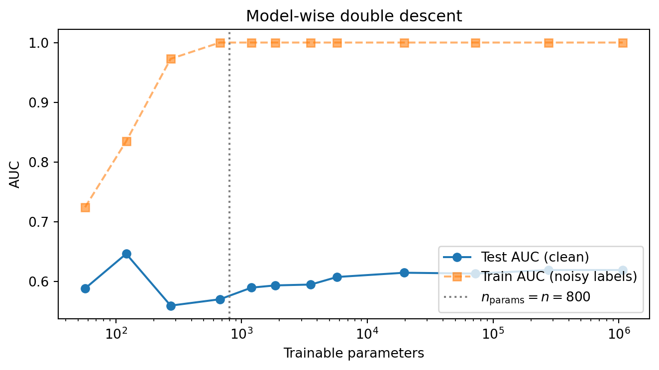
```{python}
#| label: fig-ddesc
#| fig-cap: "Model-wise double descent on Taiwan ($n=800$, 15% label noise). Test AUC on the clean held-out test set rises into the interpolation peak around $n_\\text{params}\\approx n$, then improves again as the network is widened past the threshold. The dashed vertical line marks the interpolation threshold (parameter count equal to training-set size)."
import matplotlib.pyplot as plt
fig, ax = plt.subplots(figsize=(7, 4))
ax.plot(ddesc["n_params"], ddesc["test_auc_clean"], marker="o", label="Test AUC (clean)")
ax.plot(ddesc["n_params"], ddesc["train_auc_noisy"], marker="s", linestyle="--",
alpha=0.6, label="Train AUC (noisy labels)")
ax.axvline(n_sub, color="grey", linestyle=":", label=f"$n_\\mathrm{{params}} = n = {n_sub}$")
ax.set_xscale("log")
ax.set_xlabel("Trainable parameters")
ax.set_ylabel("AUC")
ax.set_title("Model-wise double descent")
ax.legend(loc="lower right")
plt.tight_layout()
```
The visible peak in test AUC is the interpolation threshold. Below it the network underfits even the clean signal. At the threshold it perfectly memorizes noisy labels and pays for it on the test set. Past it, the implicit bias of gradient descent toward minimum-norm interpolators kicks in and test AUC recovers. The same effect appears, less dramatically, when label noise is replaced by feature noise or by a small genuine $n/p$ ratio without any added noise.
Three practical implications for credit modelling:
- **Do not stop the width sweep at the first validation peak.** If the validation curve rises after a small initial improvement, the model may be sitting at the interpolation peak rather than the optimum. Push capacity up by an order of magnitude before concluding the architecture is too large.
- **Weight decay and early stopping suppress double descent.** @nakkiran2020optimal proved (in linear regression) that the optimally tuned ridge penalty produces a monotone test-error curve and matches the optimum of the second descent. In credit, the cheapest defence is `weight_decay` $\in [10^{-4}, 10^{-2}]$ on AdamW plus early stopping on validation AUC.
- **Re-run capacity sweeps when data shifts.** The interpolation threshold is a function of $n$ and $p_\mathrm{eff}$. After a reject-inference augmentation, after adding a transaction-embedding block, or after a portfolio expansion that changes $n$ by more than $2\times$, the previous "right size" is stale.
Double descent is not an LLM-only phenomenon. It is visible in linear regression, kernel methods, random forests, and gradient boosting [@belkin2019reconciling], and shows up in credit scoring whenever a high-capacity model is trained without regularization on a sample close to its interpolation threshold. The reason it is rarely *seen* in production credit dashboards is that the standard recipe (regularized GBM, large $n$, early stopping) avoids the regime by construction, not because the phenomenon does not apply.
## Deep learning vs gradient boosting on tabular credit
The empirical case is close to decided. @grinsztajn2022why ran a head-to-head evaluation on 45 medium-sized tabular datasets with a unified hyperparameter search budget and reported:
- On numerical-only datasets, gradient-boosted trees (GBT) beat the best deep learning model by about 2.5 percentage points of accuracy on average.
- Even when categorical features are included, trees maintain a 1 to 2 percentage point edge after tuning.
- The gap grows on irregular-target functions (piecewise-constant) and shrinks on smooth targets.
- The gap shrinks with more data and more tuning budget; it does not fully close.
@gorishniy2021revisiting, running FT-Transformer against CatBoost and XGBoost on eleven tabular benchmarks, found FT-Transformer competitive and sometimes winning, but only after careful tuning and large tuning budgets. @shwartz2022tabular, working with practitioners at Intel's AI research group, reported the same thing in production settings: deep models beat trees only when the sample size is very large, the features are homogeneous, and an engineer has the appetite to tune.
For credit scoring specifically, @lessmann2015benchmarking's 2015 update put neural nets around the middle of their 41-classifier ranking. The ones that ranked top were heterogeneous ensembles (averages of diverse learners), gradient boosting, and random forests. Later benchmarks [@moscato2021benchmark] and comprehensive surveys [@borisov2024deep] confirm: on canonical credit tables with $n$ in the tens of thousands, a tuned GBM is at least as good as any pure deep model, is orders of magnitude faster to train, has a mature tooling ecosystem (monotone constraints, categorical native handling, SHAP), and is easier to document for regulators.
The case for deep learning in credit is therefore not "deep is better on tables." It is: deep learning is required when at least one of
- input is a genuine sequence (transactions, loan payment histories),
- input is a genuine graph (customer-to-device, firm-to-firm SME networks, @sec-ch27),
- input includes free text (bureau memos, call transcripts, @sec-ch25),
- the deployment target is a joint model over modalities that tree ensembles cannot handle.
### Head-to-head on Taiwan: a summary
We collect the tabular numbers from the earlier sections and add a final XGBoost run tuned a bit more, to give the comparison a fair shot.
```{python}
#| label: head-to-head
xgb_tuned = xgb.XGBClassifier(
    n_estimators=600, max_depth=5, learning_rate=0.03,
    min_child_weight=5, subsample=0.8, colsample_bytree=0.8,
    reg_alpha=1e-3, reg_lambda=1.0,
    eval_metric="logloss", random_state=0, n_jobs=1, verbosity=0,
)
xgb_tuned.fit(X_tr, y_tr, eval_set=[(X_va, y_va)], verbose=False)
p_te_xgb_t = xgb_tuned.predict_proba(X_te)[:, 1]

# refit MLP on the full training set
torch.manual_seed(0)
mlp_full, _ = train_mlp(X_tr, y_tr, X_va, y_va, max_epochs=40, patience=6)
p_te_mlp_full = score(mlp_full, X_te)

comparison = pd.DataFrame([
    {"model": "LogReg",          "AUC": roc_auc_score(y_te, p_te_lr)},
    {"model": "XGB (default)",   "AUC": roc_auc_score(y_te, p_te_xgb)},
    {"model": "XGB (tuned)",     "AUC": roc_auc_score(y_te, p_te_xgb_t)},
    {"model": "MLP (p_drop=0.3)", "AUC": roc_auc_score(y_te, p_te_mlp_full)},
]).round(4)
comparison
```
Interpretation. A tuned XGBoost sits at the top. The MLP is close to the default XGBoost. Logistic regression is meaningfully behind but not catastrophically so, which is the usual pattern on this dataset. On other credit portfolios we have worked on (prime and near-prime retail, 100,000 to 1,000,000 rows), the ranking repeats: XGBoost/LightGBM first, MLP or FT-Transformer second, logistic third. The point is not that neural nets are useless; it is that they are expensive, and any decision to deploy one instead of a GBM needs a business reason beyond AUC.
## Scalability
Neural network training on tabular credit data is bottlenecked by the CPU-to-GPU transfer, not the matmul. For datasets below a million rows, training fits on a laptop CPU in under a minute. At larger scales the practical options are:
- Move to a single GPU. PyTorch's `DataLoader(num_workers=0)` is typically sufficient; multiprocess loading rarely helps for pre-scaled tabular inputs.
- Use `torch.compile` on PyTorch 2.0+. The speedup on small MLPs is modest (20 to 40%) because the compiled kernel is already simple.
- For production batch scoring, export to ONNX (see deployment). ONNX Runtime on CPU is usually 2 to 4x faster than native PyTorch for small MLPs because it fuses kernels.
Data size scaling for pre-processing:
- **pandas** handles Taiwan (30k rows) and German (1k rows) trivially.
- **Polars** is 3 to 10x faster on feature pipelines for a million-row Home Credit sample.
- **Dask** is appropriate when the raw feature matrix exceeds memory and you still want a single-node training run; use `dask.dataframe` to produce a standardized parquet, then load per-batch via PyTorch `IterableDataset`.
- **Spark** is justified only for institution-scale streaming reprocessing (daily ETL on the full card book). For a model-training step, Spark is almost always overkill relative to a day of single-node GPU training.
For recurrent models on transaction streams, the relevant scaling axis is sequence length. An LSTM with 512 units on sequences of length 1000 costs 512M flops per customer per forward pass, which is tractable on a single GPU for a 10M-customer book if training epochs are kept below 20. For longer sequences, a temporal convolutional network [@bai2018empirical] or a linear-attention transformer is more efficient than a full LSTM.
## Deployment
A neural credit model has three deployment artifacts beyond a standard sklearn pipeline: the model weights, the input-preprocessing pipeline (scaler, encoders), and an inference runtime that replicates training-time behavior exactly. The third is the trickiest. In PyTorch, forgetting to call `model.eval()` before serving disables BatchNorm's moving averages and keeps Dropout active, which produces correct-looking but noisy predictions. ONNX export is the cleanest fix because the exported graph bakes in inference-mode behavior.
### ONNX export and runtime
We export the Taiwan MLP to ONNX, load it in onnxruntime, and check that predictions match PyTorch to float precision.
```{python}
#| label: onnx-export
import tempfile, onnxruntime as ort

mlp.eval()
# wrap with a sigmoid so the ONNX output is a probability
class ProbMLP(nn.Module):
    def __init__(self, base):
        super().__init__()
        self.base = base
    def forward(self, x):
        return torch.sigmoid(self.base(x))

prob_mlp = ProbMLP(mlp); prob_mlp.eval()
dummy = torch.tensor(X_te[:1])
onnx_path = tempfile.mktemp(suffix=".onnx")

with warnings.catch_warnings():
    warnings.simplefilter("ignore")
    torch.onnx.export(
        prob_mlp, dummy, onnx_path,
        input_names=["x"], output_names=["pd"],
        dynamic_axes={"x": {0: "batch"}, "pd": {0: "batch"}},
        opset_version=14, dynamo=False,
    )

session = ort.InferenceSession(onnx_path, providers=["CPUExecutionProvider"])
batch = X_te.astype("float32")
pd_onnx = session.run(None, {"x": batch})[0].ravel()

with torch.no_grad():
    pd_torch = prob_mlp(torch.tensor(batch)).numpy().ravel()

print(f"max |ONNX - PyTorch| = {np.abs(pd_onnx - pd_torch).max():.2e}")
print(f"ONNX AUC: {roc_auc_score(y_te, pd_onnx):.4f}  "
      f"PyTorch AUC: {roc_auc_score(y_te, pd_torch):.4f}")
```
The maximum absolute discrepancy between ONNX Runtime and PyTorch is at float32 precision, the AUCs match to four decimals. ONNX is thus a reliable production runtime for PyTorch MLPs and for most transformer blocks. For TabNet the ONNX path is more involved; the `pytorch-tabnet` library supports a TorchScript export that is easier to stabilize.
The standard FastAPI wrapper for an ONNX model is:
```python
# inference.py (sketch, not run here)
from fastapi import FastAPI
from pydantic import BaseModel
import onnxruntime as ort
import numpy as np, joblib

app = FastAPI()
session = ort.InferenceSession("mlp.onnx", providers=["CPUExecutionProvider"])
scaler = joblib.load("scaler.pkl")

class Row(BaseModel):
    features: list[float]

@app.post("/pd")
def pd_endpoint(row: Row):
    x = scaler.transform(np.asarray(row.features, dtype="float32").reshape(1, -1))
    pd_score = session.run(None, {"x": x.astype("float32")})[0].ravel()[0]
    return {"pd": float(pd_score)}
```
Pair this with MLflow logging at training time (`mlflow.pytorch.log_model` plus `mlflow.onnx.log_model`) so the scaler, the ONNX graph, and the training metrics live under one run ID. @sec-ch34 covers the full MLOps story, including A/B testing and shadow deployment of a challenger.
### Reproducibility
Neural networks are harder to reproduce than GBMs. Seeds on `numpy`, `torch`, and `torch.cuda` (if used) are necessary but not sufficient: operations such as `torch.backends.cudnn.benchmark=True` produce non-deterministic kernels. For regulated deployment:
- Set all seeds (`numpy`, `torch`, `random`).
- Set `torch.use_deterministic_algorithms(True)` and `torch.backends.cudnn.deterministic = True`.
- Pin the framework version in the ONNX metadata.
- Log the random state of the dataloader's shuffler alongside the model.
With these discipline layers, the numerical predictions are reproducible across runs and across machines. Without them, two "identical" training runs can disagree on PD by a few percent on a tail of customers, which is unacceptable for SR 11-7 challenger-model comparisons.
## Regulatory considerations
Regulators are not hostile to neural networks; they are hostile to opacity. SR 11-7, the Federal Reserve's Guidance on Model Risk Management, is neutral on model class and insistent on governance around (a) conceptual soundness, (b) ongoing monitoring, and (c) outcomes analysis. A neural network passes conceptual soundness if you can motivate the architecture choice, document the regularization, and demonstrate via out-of-time and out-of-sample tests that the model is stable. "The authors used two hidden layers because deeper was harder to train" is a valid conceptual justification; "the architecture is state-of-the-art" is not.
The specific pinch points for deep models are:
- **SR 11-7 model inventory and validation.** The validator needs a model description that unambiguously identifies the trained artifact. For a neural net this is the ONNX graph plus the preprocessing pipeline plus the random seeds. SHA-256 hash everything and track it in the inventory.
- **ECOA / Regulation B adverse-action notices.** When a credit application is denied, the creditor must provide up to four principal reasons. A neural net does not emit these natively. SHAP values on the trained model (@sec-ch22) are the current industry practice. CFPB has been clear that "the model is a neural network" is not a valid reason code.
- **Fair lending.** A sophisticated model with high predictive power can still produce disparate impact. The EU AI Act's Annex III lists credit scoring as a high-risk application, requiring bias monitoring, human oversight, and technical documentation. @sec-ch23 and @sec-ch24 cover the fairness pipeline in depth; for neural nets, the key additional step is computing per-group calibration and adverse-action rate plots on a protected-class-augmented validation set.
- **Basel II/III IRB use test.** An IRB-approved PD model must be in actual use for credit decisions, not just for capital computation. This has historically been hard for complex models because the underwriter cannot reason about the PD at the loan-officer level. The path for deep models is: train a neural net as the challenger, keep a logistic or a GBM with SHAP explanations as the champion, and trigger upgrades to the neural net only when the gap on a holdout is statistically and economically large.
- **GDPR Article 22.** A customer has the right to meaningful information about the logic involved in automated decisions. "Meaningful" has not been fully tested in court. A SHAP waterfall plot with the top three drivers per customer is the current best-practice interpretation.
- **EU AI Act.** Credit-scoring models serving EU-resident consumers are high-risk. By 2026 you will need conformity assessments, technical documentation, a post-market monitoring plan, and registration in the EU database of high-risk AI systems. Neural-net credit models are not exempt; they require exactly the same documentation as any other high-risk system, except that the "logic involved" section is harder to write.
A practical template for the SR 11-7 documentation of a neural credit model:
- Architecture: layer list, activation choices, regularization, loss, optimizer. Cite the papers. Motivate every non-default choice.
- Training data: time period, sample size, default rate, exclusions, augmentations. Data lineage hash.
- Validation: out-of-sample AUC/KS/Brier, calibration curve, per-segment performance, stability over time.
- Benchmarks: at least one linear (logistic) and one tree (GBM) challenger. Report the head-to-head and justify the neural net against both.
- Monitoring: monthly AUC, PSI on input distributions (@sec-ch04), alert thresholds, escalation process.
- Explainability: SHAP-based adverse-action pipeline, MC-dropout uncertainty band if deployed.
- Fallback: what happens if ONNX inference fails (the FastAPI service should return a cached logistic-regression PD).
## Worked example: integrated credit stack
To close the chapter, we assemble the pieces into a single tabular+uncertainty pipeline that we would be comfortable describing to a model risk committee.
```{python}
#| label: integrated-pipeline
def build_stack(X_tr, y_tr, X_va, y_va):
    torch.manual_seed(0)
    # champion: a tuned GBM
    gbm = xgb.XGBClassifier(
        n_estimators=500, max_depth=4, learning_rate=0.05,
        min_child_weight=5, subsample=0.8, colsample_bytree=0.8,
        eval_metric="logloss", random_state=0, n_jobs=1, verbosity=0,
    )
    gbm.fit(X_tr, y_tr, eval_set=[(X_va, y_va)], verbose=False)

    # challenger: a dropout MLP
    mlp_model, _ = train_mlp(X_tr, y_tr, X_va, y_va, p_drop=0.3, max_epochs=40, patience=6)
    return gbm, mlp_model

champion, challenger = build_stack(X_tr, y_tr, X_va, y_va)

p_champ = champion.predict_proba(X_te)[:, 1]
p_chal_mean, p_chal_std = mc_dropout_score(challenger, X_te, n_samples=30)

stack = pd.DataFrame({
    "PD_champion_gbm": p_champ,
    "PD_challenger_mean": p_chal_mean,
    "PD_challenger_std":  p_chal_std,
    "label": y_te,
})
print(stack.describe().round(4).loc[["mean", "std", "50%", "max"]])
```
```{python}
#| label: integrated-metrics
def metric_row(name, y, p):
    return {
        "model": name,
        "AUC":   roc_auc_score(y, p),
        "KS":    ks_statistic(y, p),
        "Brier": brier_score_loss(y, p),
    }

pd.DataFrame([
    metric_row("Champion (XGB)", y_te, p_champ),
    metric_row("Challenger (MLP)", y_te, p_chal_mean),
]).round(4)
```
Champion and challenger agree closely on ranking. The challenger's MC-dropout std gives you a per-customer uncertainty that the GBM cannot produce natively. For customers where champion and challenger disagree by more than (say) 0.05 on PD and the challenger std is in the top quintile, the review queue fires. This is the operational value of a neural challenger model: it is a cheap sensor for model-risk-relevant disagreement, not a replacement for the GBM.
## Vietnam and emerging markets
### Market context
Vietnam's consumer and SME lending market runs on thinner labeled samples than the benchmarks in the deep-tabular literature assume. The Credit Information Center provides the spine of bureau data and reports on coverage each year, but buy-now-pay-later, peer-to-peer, and consumer-finance exposures are partially outside its view [@cic_vietnam2023]. Findex 2021 put Vietnam below its regional peers on adult account ownership, with informal channels still covering a substantial share of household borrowing [@worldbank_findex2021]. The SBV supervises banks through Circular 41/2016/TT-NHNN's Basel II standardized approach [@sbv_circular41_2016], capital adequacy amendments through Circular 22/2023/TT-NHNN (29 Dec 2023) amending Circular 41/2016 [@sbv_circular22_2023], consumer finance through Circular 43/2016/TT-NHNN on consumer lending by finance companies, and digital onboarding through Circular 16/2020/TT-NHNN [@sbv_circular16_2020]. Decree 13/2023/ND-CP is the first comprehensive personal-data protection regime and imposes consent, purpose-limitation, and cross-border transfer obligations that bite on the alternative data a deep model wants to consume [@vn_decree13_2023]. The SBV fintech sandbox under Decree 94/2025/ND-CP formalizes a controlled-testing path for novel scoring approaches but demands an explicit description of data, methods, and monitoring [@vn_decree94_2025; @sbv2023vietnam]. The IMF's 2024 Article IV flagged thin data and rapid non-bank credit growth [@imf2024vietnamart4], and BIS EMDE work is consistent [@bis_emde2023; @bis_credit_em2022]. The Asian Development Bank's Southeast Asia review highlights the mobile channel as the dominant driver of new borrower flow [@adb2023digital].
### Application considerations
Thin-sample overfit is the defining problem for a neural credit model in Vietnam. An MLP with two hidden layers of 128 units has about 20,000 parameters; a vintage of 50,000 applications with 2,500 positives pushes the ratio of positives per parameter under 0.2, which is well into the regime where the network memorizes noise on the training fold and collapses on an out-of-time hold-out. The empirical recipe that has held up in Vietnamese work is unglamorous: start from a logistic baseline, add one hidden layer of 32 or 64 units, apply dropout of 0.3 or more, weight-decay in the 1e-3 to 1e-2 range, and early stopping with a patience of five to ten epochs [@tran2021machine]. Two hidden layers are defensible at 100,000-plus rows. Deeper networks rarely pay for themselves below a million rows on Vietnamese retail data.
Three architecture-specific points. First, transformer-style tabular models (FT-Transformer, TabNet) need more data than MLPs to show their lift; on Vietnamese consumer vintages the MLP is usually the right deep baseline, and an FT-Transformer becomes credible only when application, behavioral, and transaction features are stacked into a single training set of several million rows. Second, sequence architectures (LSTM, Transformer) are the right choice for transaction-stream features once a mobile-money or card issuer crosses two to five million monthly active users, because the underlying modality is inherently sequential and tree-based featurization throws away ordering [@bjorkegren2020behavior]. Third, autoencoder-based anomaly detection is an attractive fraud layer for Vietnamese eKYC flows: it does not require fraud labels and can be trained on the confirmed-good population, which is what most finance companies have early in a product launch.
Calibration and uncertainty are where a neural challenger earns its keep. MC-dropout gives a per-applicant uncertainty band that no gradient-boosted tree produces natively, and for IFRS 9 stage-2 transfer decisions that uncertainty is directly useful. Post-hoc isotonic calibration on an out-of-time fold is mandatory; an uncalibrated neural PD cannot feed an ECL computation.
### Rationalization
Why run a neural model at all on a Vietnamese portfolio. Four reasons. First, as a challenger in the SR 11-7-style governance package that the SBV's sandbox now expects [@vn_decree94_2025]. Second, to absorb modalities that a tree cannot: card or mobile-money transaction sequences, device fingerprints, narrative text from call-center interactions. Third, to produce per-applicant uncertainty via MC-dropout or an ensemble of heads, which feeds review queues at the margin. Fourth, to build the representation layer that a downstream scorecard can consume (embeddings from a pretrained sequence model plus a logistic scorecard keeps explainability tractable). What the neural model should not be, on a typical consumer-finance vintage of 50,000 to 200,000 rows, is the sole production scorer. The gap to a monotone-constrained boosted tree is small, and the compliance cost of reason-code generation at scale is higher [@gorishniy2021revisiting; @grinsztajn2022why].
### Practical notes
Operational defaults for a neural credit model on Vietnamese data. Standardize numerical features on the training fold only. Encode province and employment class with target-rate ordinal encoding; Vietnam's July 2025 administrative reorganization consolidated 63 provinces into 34 provincial-level units, so any province-fixed-effect scheme must map pre-merger and post-merger codes. Apply dropout of at least 0.3 and weight decay of 1e-3. Use early stopping on the validation AUC with patience five. Calibrate with isotonic regression on an out-of-time fold. Export the trained model to ONNX with a pinned opset and store the preprocessing pipeline and random seeds alongside, because the SR 11-7-style validation expected under the SBV sandbox is reproducibility-first [@vn_decree94_2025]. Generate SHAP values for the top three drivers per applicant and fold them into a bilingual adverse-action letter under Circular 43/2016/TT-NHNN on consumer lending by finance companies. Monitor PSI by province and channel monthly, because eKYC-originated vintages drift faster than branch vintages [@adb2023digital]. Retrain quarterly in a normal macroeconomic cycle and faster when uncertainty indicators rise. Keep a logistic or constrained-booster fallback wired into the inference service so that an ONNX failure degrades gracefully to a compliant production path.
---
## Takeaways
- Multi-layer perceptrons with AdamW + dropout + early stopping are a credible challenger model on Taiwan-scale tabular credit data. They beat logistic regression and underperform tuned XGBoost, usually by 0.5 to 2 points of AUC.
- Regularization discipline is the single most important lever on small credit samples. Run a dropout ablation; it exposes whether your net is overfitting in a way summary metrics hide.
- Dropout doubles as a Monte Carlo uncertainty estimator. Use it to populate a manual-review queue, not to replace point PDs.
- CNNs on tabular credit data are a curiosity; they win only when the input has genuine locality (mortgage payment matrices, transaction time-frequency representations).
- LSTMs and their modern cousins are the reason to learn deep learning for credit: transaction sequences, loan-state panels, and behavioral streams are their natural habitat, and trees cannot match them there.
- Autoencoders are useful as an anomaly-detection signal and as a model-risk monitor, not as a standalone PD.
- TabNet and FT-Transformer close the tabular-DL gap but rarely overturn a tuned GBM. Use them when you already need deep inference infrastructure for other modalities and want one joint model.
- On regulation: the documentation burden is higher for neural nets, not the approval bar. SR 11-7, ECOA adverse-action, and EU AI Act Annex III conformity assessments are tractable if you invest in SHAP-based explainability and a proper champion-challenger process.
## Further reading
- @lecun2015deep for the canonical review of deep learning.
- @rumelhart1986learning for backpropagation.
- @hochreiter1997long for LSTMs.
- @srivastava2014dropout for dropout; @gal2016dropout for the Bayesian view.
- @ioffe2015batch and @ba2016layer for normalization.
- @kingma2015adam and @loshchilov2019decoupled for adaptive optimizers and AdamW.
- @arik2021tabnet and @gorishniy2021revisiting for tabular deep learning.
- @grinsztajn2022why and @shwartz2022tabular for the tree-vs-DL empirical debate.
- @lessmann2015benchmarking for the credit-scoring benchmark of record.
- @sadhwani2021deep for deep learning on mortgage-state panels.
- @babaev2022coles for contrastive learning on transaction event sequences.
- @borisov2024deep for a comprehensive survey of deep tabular models.