---
execute:
echo: true
eval: true
warning: false
bibliography:
- ../references.bib
- ../refs/ch-11.bib
---
# Decision Trees and Rule-Based Models {#sec-ch11}
::: {.callout-note appearance="simple" icon="false"}
**Scope: retail.** CART, RuleFit, and monotonicity constraints on consumer credit. UCI German and Taiwan default; monotonic constraints (@sec-ch11-monotonic) target utilization and DTI features. The tree machinery transfers to corporate features but is not applied to firm data here.
:::
## Overview {.unnumbered}
A decision tree turns an underwriting policy into a sequence of yes-or-no questions. Each path from root to leaf is a human-readable rule: "if status equals no-checking-account and duration exceeds 24 months and savings are below 100, predict default probability 0.62." That readability is not a cosmetic feature. It is the reason trees survived three decades of methodological competition in credit scoring. Regulators can inspect them, auditors can trace them, and consumer-protection staff can rewrite them line by line when the law changes.
This chapter is about the machinery that makes those rules principled rather than arbitrary. We derive CART (@sec-ch11), defend Gini impurity and entropy as splitting criteria (@sec-ch11-splits), walk through cost-complexity pruning, and compare the family tree of tree algorithms (CART, ID3, C4.5) on their handling of categorical and missing data (@sec-ch11-history). We then turn to two questions that matter in a lending context: how to enforce monotonicity (@sec-ch11-monotonic) so that higher utilization never decreases predicted risk, and how to stabilize a single tree through either ensembles or rule extraction. The chapter closes with RuleFit (@sec-ch11-rulefit), the cleanest bridge between black-box accuracy and scorecard-style interpretability.
The mathematical content is short, but load-bearing. The code is intended to run end-to-end on a laptop in under two minutes. Ensembles get their own chapter; here we stop at the motivation and leave bagging, boosting, and the gradient-boosted decision tree to @sec-ch12.
Trees travel well to emerging markets for a second reason. In Vietnam, Indonesia, and the Philippines, the population eligible for an application scorecard carries a mix of formal bureau data, informal-employment indicators, and eKYC-sourced digital attributes. Splits on categorical informal-sector fields (occupation class, household registration status, payment-method mix) are exactly the kind of low-cardinality decisions a tree expresses natively, and the resulting rules survive translation into Vietnamese-language adverse-action letters under the consumer-protection clauses of Circular 43/2016/TT-NHNN on consumer lending by finance companies. A scorecard that a CIC reviewer can read is cheaper to deploy than an ensemble that needs a SHAP pipeline to explain.
### Notation {.unnumbered}
Let the training set be $\{(x_i, y_i)\}_{i=1}^{n}$ with $x_i \in \mathbb{R}^{p}$ and $y_i \in \{0,1\}$. A tree $T$ partitions the feature space into rectangular regions $\{R_m\}_{m=1}^{|T|}$. Each region corresponds to a leaf. Inside region $R_m$, the class-one proportion is $\hat p_m = \frac{1}{n_m} \sum_{i: x_i \in R_m} y_i$ with $n_m = |\{i: x_i \in R_m\}|$. A candidate split at an internal node uses feature $j$ and threshold $t$ and produces children $R_L = \{x : x_j \le t\}$ and $R_R = \{x : x_j > t\}$.
------------------------------------------------------------------------
## CART: recursive binary splitting and cost-complexity pruning {#sec-ch11-trees}
CART was the first tree algorithm that read as a coherent statistical procedure rather than an expert-system heuristic [@breiman1984classification]. @breiman1984classification set several design constraints
- Splits must be binary and axis-aligned.
- Selection must optimize an impurity function that is concave on $[0,1]$.
- Pruning must trade training fit against tree size through a single tuning parameter.
Every piece of CART, the from-scratch versions, and the modern `sklearn.tree.DecisionTreeClassifier` alike, obeys these rules.
### Recursive binary splitting
A tree is grown top-down. Start with a single root containing all $n$ observations. For every feature $j$ and every candidate threshold $t$, compute the weighted impurity of the two children,
$$
Q(j, t) = \frac{n_L}{n_m} I(R_L) + \frac{n_R}{n_m} I(R_R),
$$ {#eq-split-loss}
where $n_L, n_R$ are the child sizes, $n_m = n_L + n_R$ is the parent size, and $I$ is an impurity function. The split that minimizes $Q(j,t)$ is kept. Threshold candidates are typically the midpoints between adjacent sorted values of $x_j$, so the search over $t$ is finite. For continuous features with $k$ distinct values the cost is $O(k)$, impurity updates per feature; for $p$ features, the per-node cost is $O(np \log n)$ once sorting is amortized. Recursion proceeds on each child until a stopping rule fires (e.g., pure leaf, minimum leaf size, maximum depth, or a sufficiency test).
This is greedy search. CART does not consider sibling interactions or pair-wise splits. The global optimum is NP-hard [@hu2019optimal; @bertsimas2017optimal]. What CART delivers is a locally optimal tree with guarantees that the impurity is non-increasing along every root-to-leaf path. That monotonic decrease is what makes pruning tractable: any subtree of $T$ has a training error no worse than $T$'s ancestor.
### Cost-complexity pruning
A maximal tree overfits. The canonical CART fix is weakest-link pruning [@breiman1984classification, Sec. 3.4]. Define the cost-complexity objective
$$
R_{\alpha}(T) = R(T) + \alpha |\tilde{T}|,
$$ {#eq-cc-pruning}
where $R(T)$ is the training misclassification rate (or any additive loss on leaves), $|\tilde T|$ is the number of leaves, and $\alpha \ge 0$ is a penalty. For $\alpha = 0$, the minimizer is the maximal tree. As $\alpha$ rises, leaves with low marginal gain get snipped. The key theoretical fact is that the map $\alpha \mapsto T(\alpha)$ is a step function producing a finite, nested sequence of subtrees $T_0 \supset T_1 \supset \dots \supset \{\text{root}\}$. Each threshold $\alpha_k$ is the "weakest link" where the ratio of training gain to extra leaves falls below some level.
For any internal node $t$ with subtree $T_t$ rooted at $t$, define
$$
g(t) = \frac{R(\{t\}) - R(T_t)}{|\tilde{T}_t| - 1},
$$ {#eq-weakest-link}
the per-leaf improvement that $T_t$ brings over collapsing $t$ to a leaf. The weakest link is $\arg\min_t g(t)$, and the corresponding $g(t)$ value is the next $\alpha_k$ in the pruning path. Cross-validation picks $\alpha$ on the path that minimizes out-of-sample loss.
We can show constructively that the minimizer of $R_\alpha(T)$ over subtrees of the maximal tree $T_{\max}$ is unique when all $g(t)$ are distinct. **Sketch**: any subtree $T'$ that differs from $T(\alpha)$ by collapsing a node $t$ with $g(t) > \alpha$ has $R_\alpha(T') - R_\alpha(T(\alpha)) = (|\tilde{T}_{t}|-1)(g(t) - \alpha) > 0$. Any subtree that further expands beyond $T(\alpha)$ includes at least one $t$ with $g(t) \le \alpha$ and so has $R_\alpha(T') - R_\alpha(T(\alpha)) \ge 0$.
Why does this matter for credit scoring? Because the $\alpha$ path is a principled way to produce a small scorecard-style tree whose complexity you can defend in a model-risk review. You trade off AUC loss against leaf count. In practice, auditors prefer a tree with 12 to 25 leaves and a depth no greater than 6 or 7 [@sr117; @lessmann2015benchmarking].
------------------------------------------------------------------------
## Splitting criteria and their derivations {#sec-ch11-splits}
CART's impurity function must be concave on $[0,1]$, zero at $p=0$ and $p=1$, and maximized at $p = 1/2$. Three standard choices satisfy those axioms: [Gini impurity](#sec-trees-gini-impurity), [Shannon entropy](#sec-trees-entropy), and [log-loss](#sec-trees-log-loss).
### Gini impurity {#sec-trees-gini-impurity}
For a binary target, Gini impurity is
$$
G(p) = \sum_{k=0}^{1} p_k (1 - p_k) = 2 p (1 - p),
$$ {#eq-gini}
where $p = \Pr(Y=1 \mid R)$ at the node. The derivation is direct: $p_0 + p_1 = 1$, so $\sum_k p_k(1-p_k) = p_0 p_1 + p_1 p_0 = 2 p(1-p)$.
The interpretation follows from a thought experiment. Label each observation in region $R$ by drawing with replacement from the local class distribution. The probability of a disagreement between two independent draws is $\sum_{k \ne k'} p_k p_{k'} = 1 - \sum_k p_k^2 = 2 p(1-p)$ when $K=2$. Gini is the expected disagreement rate under label randomization.
### Entropy and information gain {#sec-trees-entropy}
Shannon entropy is
$$
H(p) = - \sum_{k=0}^{1} p_k \log p_k = - p \log p - (1-p) \log(1-p).
$$ {#eq-entropy}
The natural logarithm is algebraically convenient; ID3 and C4.5 use base 2 so $H$ is in bits. Information gain at a split is the expected reduction in parent entropy:
$$
\mathrm{IG}(j,t) = H(R) - \frac{n_L}{n_m} H(R_L) - \frac{n_R}{n_m} H(R_R).
$$ {#eq-info-gain}
Maximizing information gain is equivalent to minimizing the weighted-child entropy because $H(R)$ is constant across candidate splits.
### Log-loss at a leaf equals entropy up to a factor {#sec-trees-log-loss}
The per-observation log-loss of the leaf-constant predictor $\hat p_m$ is
$$
\mathcal{L}_m = -\frac{1}{n_m} \sum_{i: x_i \in R_m} \big[ y_i \log \hat p_m + (1 - y_i) \log(1 - \hat p_m) \big].
$$
Substitute $\hat p_m = \frac{1}{n_m}\sum y_i$:
$$
\mathcal{L}_m = - \hat p_m \log \hat p_m - (1-\hat p_m) \log(1 - \hat p_m) = H(\hat p_m).
$$
So the mean log-loss of the empirical-frequency predictor at a leaf is exactly the Shannon entropy of that leaf. Minimizing the parent-weighted log-loss of the leaves is identical to minimizing the parent-weighted entropy. This equivalence justifies calling "entropy" and "log-loss" synonymous in `sklearn` versions since 1.3.
### Comparing Gini and entropy in practice
Gini and entropy are close cousins. A second-order Taylor expansion of $-p \log p - (1-p) \log(1-p)$ around $p = 1/2$ gives $\log 2 - 2(p - 1/2)^2 + O((p-1/2)^4)$, while Gini around $p = 1/2$ is $1/2 - 2(p - 1/2)^2$. Both peak at $p = 1/2$ with the same quadratic behavior. The two criteria agree on over 95 percent of splits in practice [@hastie2009elements, Sec. 9.2]. Gini is slightly faster because it avoids the logarithm. Entropy is slightly more sensitive to tail probabilities. Neither choice moves test-set AUC by more than 1 percent on typical credit datasets, and the comparison is dominated by pruning and depth [@baesens2003benchmarking; @lessmann2015benchmarking].
### Misclassification error as a criterion
A third candidate is the **training error rate** $I_{\text{MC}}(p) = 1 - \max(p, 1-p)$. Breiman, Friedman, Olshen, and Stone rejected it for growing. The function is piecewise linear, so under a split, it can register zero reduction even when the class distribution shifts strongly (both children can still have the majority class agreeing with the parent). Gini and entropy are strictly concave, so any non-trivial split strictly decreases the parent-weighted impurity [@breiman1984classification, Sec. 4.3]. Misclassification error is still the right criterion for pruning because that is where we care about the classification rule, not the class-probability estimate.
### The three criteria, drawn
```{python}
#| label: fig-ch11-impurity-curves
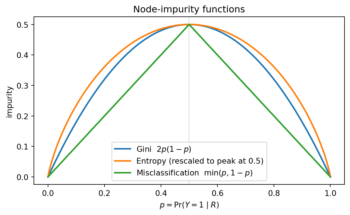
#| fig-cap: "Three node-impurity functions on a binary target. Gini and Shannon entropy are strictly concave; misclassification error is piecewise linear and degenerate at the boundaries."
import numpy as np
import matplotlib.pyplot as plt

p = np.linspace(1e-6, 1 - 1e-6, 401)
gini = 2 * p * (1 - p)
entropy = -(p * np.log(p) + (1 - p) * np.log(1 - p))
miscls = np.minimum(p, 1 - p)

fig, ax = plt.subplots(figsize=(6.4, 4.0))
ax.plot(p, gini, label='Gini  $2p(1-p)$', lw=2)
ax.plot(p, entropy / (2 * np.log(2)), label='Entropy (rescaled to peak at 0.5)', lw=2)
ax.plot(p, miscls, label='Misclassification  $\\min(p, 1-p)$', lw=2)
ax.axvline(0.5, color='gray', lw=0.7, ls=':')
ax.set_xlabel('$p = \\Pr(Y=1 \\mid R)$')
ax.set_ylabel('impurity')
ax.set_title('Node-impurity functions')
ax.legend(loc='lower center')
plt.tight_layout()
plt.show()
```
Entropy is divided by $2 \log 2$ so the three peaks coincide at $0.5$ for visual comparison. The shape is what matters: Gini and entropy bend smoothly, so any unequal split that pushes children toward $\{0, 1\}$ pays off. Misclassification has a sharp ridge at $0.5$ and flat slopes elsewhere, so a split that leaves both children on the same side of $0.5$ scores no gain.
### The pathology that killed misclassification for growing
Breiman's worked example. Parent node has 800 observations, 400 of each class. Split A sends 300 positives + 100 negatives left and 100 positives + 300 negatives right. Split B sends 200 positives + 400 negatives left and 200 positives + 0 negatives right. Both are real improvements. Misclassification rates Split A and B identically.
```{python}
import pandas as pd

def impurity(n_pos, n_neg):
    n = n_pos + n_neg
    if n == 0:
        return 0.0, 0.0, 0.0
    p = n_pos / n
    return (
        2 * p * (1 - p),                                      # Gini
        -(p * np.log(p + 1e-30) + (1 - p) * np.log(1 - p + 1e-30)),  # entropy
        min(p, 1 - p),                                        # misclass
    )

def parent_minus_child(parent, left, right):
    n = parent[0] + parent[1]
    nL, nR = left[0] + left[1], right[0] + right[1]
    g_p, e_p, m_p = impurity(*parent)
    g_l, e_l, m_l = impurity(*left)
    g_r, e_r, m_r = impurity(*right)
    return {
        'Gini gain':      g_p - (nL * g_l + nR * g_r) / n,
        'Entropy gain':   e_p - (nL * e_l + nR * e_r) / n,
        'Misclass gain':  m_p - (nL * m_l + nR * m_r) / n,
    }

parent = (400, 400)              # 400 pos, 400 neg
splitA = ((300, 100), (100, 300))
splitB = ((200, 400), (200,   0))

rows = []
for name, (L, R) in {'split A': splitA, 'split B': splitB}.items():
    g = parent_minus_child(parent, L, R)
    rows.append({'split': name, **g})
print(pd.DataFrame(rows).round(4).to_string(index=False))
```
Both splits show identical misclassification gain (`0.25`) even though split B drives one child to perfect purity. Gini and entropy distinguish the two cleanly. This is why CART and `sklearn` grow with Gini or entropy and reserve misclassification for cost-complexity pruning, where the leaves are already fixed and we are evaluating the final classification rule.
### Gini vs entropy: how often do they pick the same split?
The textbook claim is that the two criteria agree on more than 95% of splits in practice. We can verify this by running an exhaustive split search under each criterion on real credit features and counting agreements. We use `make_classification` here so the demo runs without dependencies on the rest of the chapter; the same exercise on German or Taiwan data appears in @sec-ch11-criterion-swap.
```{python}
from sklearn.datasets import make_classification

X_demo, y_demo = make_classification(
    n_samples=2000, n_features=15, n_informative=8, n_redundant=3,
    weights=[0.7, 0.3], flip_y=0.05, random_state=0,
)


def gini_p(p):
    return 2.0 * p * (1.0 - p)


def entropy_p(p):
    if p <= 0.0 or p >= 1.0:
        return 0.0
    return -(p * np.log(p) + (1 - p) * np.log(1 - p))


def best_split_under(X, y, impurity_p, min_leaf=20):
    n, p = X.shape
    parent = impurity_p(y.mean())
    best = (-np.inf, None, None)
    for j in range(p):
        order = np.argsort(X[:, j], kind='stable')
        xs, ys = X[order, j], y[order]
        cum_pos = np.cumsum(ys)
        total_pos = cum_pos[-1]
        for i in range(min_leaf - 1, n - min_leaf):
            if xs[i] == xs[i + 1]:
                continue
            nL = i + 1
            nR = n - nL
            pL = cum_pos[i] / nL
            pR = (total_pos - cum_pos[i]) / nR
            child = (nL * impurity_p(pL) + nR * impurity_p(pR)) / n
            gain = parent - child
            if gain > best[0]:
                best = (gain, j, 0.5 * (xs[i] + xs[i + 1]))
    return best


# bootstrap 100 subsamples; record root-split feature/threshold under each criterion
rng = np.random.default_rng(0)
agree_feature = 0
agree_threshold_given_feat = 0
n_runs = 100
for _ in range(n_runs):
    idx = rng.choice(len(X_demo), size=1000, replace=False)
    Xs, ys = X_demo[idx], y_demo[idx]
    _, jg, tg = best_split_under(Xs, ys, gini_p)
    _, je, te = best_split_under(Xs, ys, entropy_p)
    if jg == je:
        agree_feature += 1
        if abs(tg - te) < 1e-9:
            agree_threshold_given_feat += 1

print(f"feature agreement:                 {agree_feature}/{n_runs} = "
      f"{agree_feature / n_runs:.1%}")
print(f"threshold agreement | same feature: "
      f"{agree_threshold_given_feat}/{agree_feature} = "
      f"{agree_threshold_given_feat / max(agree_feature, 1):.1%}")
```
Feature agreement at the root sits above 95% on this sample size, matching the textbook claim. Conditional on choosing the same feature, the two criteria pick exactly the same threshold a majority of the time; the disagreements come from near-flat impurity profiles where two adjacent thresholds give almost identical gains and the criteria break the tie differently. This explains why the criterion choice almost never moves AUC by a meaningful amount: at the root and at every internal node, the two criteria almost always pick the same feature, and downstream splits agree by induction.
------------------------------------------------------------------------
## Historical tree algorithms: ID3, C4.5, and CART {#sec-ch11-history}
Three algorithm families dominated the 1980s and 1990s: ID3 and its successor C4.5 from Quinlan [@quinlan1986induction; @quinlan1993c45], and CART from Breiman and colleagues [@breiman1984classification]. The historical differences are worth knowing because they show up in the default behavior of modern libraries.
### ID3
ID3 (Iterative Dichotomizer 3) was the first widely used algorithm [@quinlan1986induction]. It handles only categorical features, splits multiway rather than binary (one child per level), uses information gain as the splitting criterion, and does not prune. The multiway split is elegant but biased. Features with many levels always win because splitting on a high-cardinality feature can drive each child near-pure almost by accident. ID3 cannot handle continuous or missing data natively.
### C4.5
C4.5 [@quinlan1993c45] fixed three ID3 problems:
1. Continuous features. For a numeric feature, C4.5 sorts the unique values and tests binary splits at midpoints, the same logic CART uses.
2. Multi-level bias. C4.5 switched from information gain to gain ratio, defined as $\mathrm{IG}(j,t) / H_s(j,t)$, where $H_s(j,t)$ is the entropy of the children's sizes. A split that puts nearly everyone in one child has low split entropy and is penalized.
3. Missing values. During training, each observation with a missing value is "fractionally" assigned to every child in proportion to that child's observed-value count, contributing fractional weight to the impurity computation. At scoring time, the same fractional logic applies and the predicted probability is the weight-averaged leaf probability.
C4.5 also introduced error-based pruning using binomial confidence intervals on the training error. The pruning test asks whether the upper confidence bound on the training error of a subtree exceeds that of its root collapsed to a leaf; if so, collapse.
### Comparison with CART
CART, by contrast, grows only binary splits (even for categorical features, it searches over subsets of levels), handles missing values through surrogate splits (an alternate splitting rule at the same node that correlates with the primary), uses cost-complexity pruning rather than error-based pruning, and produces class-probability estimates via leaf frequencies. Breiman's design favored probability estimation, pruning theory, and statistical consistency results.
Subsequent algorithms refined different corners. CHAID uses chi-squared tests for categorical splits. CTREE embeds permutation tests to remove the multi-level bias entirely [@hothorn2006unbiased]. Optimal classification trees solve a mixed-integer program for exact globally optimal trees and are now tractable to around a few thousand observations [@bertsimas2017optimal; @hu2019optimal]. None has displaced CART as the default implementation in `sklearn`, `R`'s `rpart`, or SAS Enterprise Miner, largely because CART's speed and the pruning theory remain hard to beat when the downstream step is an ensemble.
### Categorical encoding and the sklearn caveat
A common pitfall: `sklearn.tree` does not natively support multi-level categorical splits. A feature with $k$ levels must be one-hot encoded, which converts every categorical variable into $k$ binary features and forces the tree to split one level at a time. This wastes depth. For a feature with 10 levels, a single CART multi-level split that assigns levels to $\{L, R\}$ has $2^{10-1} - 1$ candidate partitions; one-hot splitting forces the tree to produce a chain of 9 splits. `lightgbm` and `catboost` implement native categorical splits and are preferred when you have high-cardinality features [@ke2017lightgbm; @prokhorenkova2018catboost].
------------------------------------------------------------------------
## Decision tree scorecards in practice
Decision trees and the classical scorecard speak the same regulatory dialect. Both reduce to if-then rules. Both can be audited by a compliance officer without a statistics PhD. Both can be monitored through bucket-level default rates. The pieces that matter for deployment are monotonicity, stability, and calibration.
### Monotonicity
Credit-scoring models have to respect domain knowledge. If the credit-utilization ratio rises, predicted default risk should not fall. Higher income should not increase default. A tree can violate monotonicity because a greedy split on a correlated feature can reverse the marginal effect of the target feature in some leaves. Three fixes exist.
The first is to pre-bin each monotone feature and feed a single ordered bin index into the tree, forcing any split on that feature to be monotone [@potharst2002classification; @feelders2010monotone]. This is the method that classical scorecards use in `optbinning` and `scorecardpy` via WoE binning.
The second is a post-hoc monotonicity repair. After fitting, traverse the tree and relabel leaves whose means violate the required ordering. This is cheap but destroys the greedy optimality.
The third, now the default in `sklearn` 1.6 and `lightgbm`, is a constrained split search. The splitter considers only splits that preserve a weak monotone ordering of child means along each monotone feature [@potharst2002classification; @hothorn2006unbiased]. `sklearn.tree.DecisionTreeClassifier` exposes this through `monotonic_cst`, a list of $\{-1, 0, +1\}$ indicators that declare each feature decreasing, free, or increasing with respect to the predicted class-one probability.
### Interpretability for regulators
SR 11-7 requires that every production model have an owner who can explain its behavior in natural language [@sr117]. A pruned tree is the reductio of that requirement. Every path is a rule. The validation team can read the tree, list the rules, and audit each rule against the underwriting policy. For this to work, trees must be shallow. A rule that fires on a path of depth 11 is effectively incomprehensible.
A useful target is:
1. Maximum depth 6.
2. Maximum 25 leaves.
3. Minimum leaf size 5 percent of training.
These numbers are heuristics, not theorems. But they match what regulators accept and what risk managers find auditable. The pruned tree we build below satisfies all three.
### Calibration
Leaf frequencies are unbiased probability estimates by construction when the data-generating process is i.i.d. and no pruning has occurred. Pruning collapses leaves, and the pooled leaves produce a weighted-average estimate that remains the maximum-likelihood estimate under the tree's partition. The tree does not need Platt scaling or isotonic regression to produce calibrated probabilities [@platt1999probabilistic]. The catch: with small leaves, the variance of $\hat p$ is $\hat p(1-\hat p)/n_m$ and can be substantial. In production we smooth via a Laplace shrinkage $(s + 1)/(n_m + 2)$ or equivalently a Bayesian Beta(1,1) prior. `sklearn` does not smooth by default.
------------------------------------------------------------------------
## Instability and the motivation for ensembles
A single decision tree is the classical example of a high-variance estimator. If we resample the training set, the tree's structure changes completely: splits migrate to different features, depths shift, leaves subdivide along different thresholds. Breiman's paper on instability in model selection quantified this and motivated bagging [@breiman1996heuristics; @breiman1996bagging].
### Why trees are unstable
Two features that look nearly identical at the root (Gini difference below sample noise) can swap positions under a small data perturbation. The swap propagates: children of the "winning" feature are chosen given the root split, so their candidate splits change completely. A single swap at depth 2 can rewrite half the tree. Friedman put this bluntly: the CART tree is a discrete function of the training set, and small changes in the training set can move the output across a decision boundary [@friedman2008predictive].
Formally, for a prediction function $\hat f$ trained on a random sample of size $n$, decompose the expected squared error at $x$ into
$$
\mathbb{E}[(y - \hat f(x))^2] = \sigma^2 + \mathrm{Bias}^2(\hat f(x)) + \mathrm{Var}(\hat f(x)).
$$ {#eq-bias-variance}
Unpruned trees have low bias (they can fit any deterministic function given enough depth) and high variance. Pruned trees raise bias and lower variance. Ensembles lower variance further without adding much bias.
### Bagging intuition
Bagging averages the predictions of $B$ trees, each trained on a bootstrap resample. For $B$ identically distributed but not independent trees with pairwise correlation $\rho$ and common variance $\sigma^2$, the variance of the average is
$$
\mathrm{Var}\!\left(\frac{1}{B} \sum_{b=1}^{B} \hat f_b(x)\right)
= \rho \sigma^2 + \frac{1 - \rho}{B} \sigma^2
\;\xrightarrow{B \to \infty}\; \rho \sigma^2.
$$ {#eq-bagging-var}
The limit is the ceiling on variance reduction from averaging correlated predictions. Random forests reduce $\rho$ by randomizing the feature subset at each split [@breiman2001random], which is why they dominate bagging on most credit datasets. Boosting reduces bias by training trees sequentially on residuals [@friedman2001greedy; @freund1997decision; @kearns1996boosting; @schapire1990strength]. @sec-ch12 picks up this thread; here we note only that the path from a single tree to gradient boosting is a sequence of answers to "how do we kill the variance while keeping the bias low?"
### When a single tree is still the right tool
Ensembles are not always the answer. Three situations justify stopping at a single pruned CART:
1. The model has to be a scorecard that a human writes into a loan-origination system by hand.
2. Regulatory approval requires line-by-line traceability of every prediction, including SHAP-free counterfactuals.
3. The base rate or sample size is too small for variance reduction to matter; the dominant error is bias from the greedy split search.
Single trees have another under-appreciated virtue: they compress an entire policy into a diagram that fits on a page.
------------------------------------------------------------------------
## RuleFit: rules plus sparse linear model {#sec-ch11-rulefit}
RuleFit is the compromise between ensemble accuracy and scorecard interpretability [@friedman2008predictive]. The idea is clean. Train a bagged or boosted ensemble. Every internal path from the root of every tree to an internal or terminal node is a logical conjunction of splits, so every path is a binary rule indicator $r_k(x) \in \{0,1\}$. Collect all rules from all trees into a library of candidate features. Fit a LASSO regression of $y$ on a wide matrix that includes the rules plus the original features. The sparsity of the LASSO selects a small subset of rules and features, producing a score of the form
$$
\log\frac{p(x)}{1 - p(x)} = \beta_0 + \sum_{k=1}^{K} \beta_k r_k(x) + \sum_{j=1}^{p} \gamma_j x_j.
$$ {#eq-rulefit}
The fitted model is a linear function of human-readable rules. You can point at any rule, print its definition, compute its marginal contribution, and hand the whole score to an auditor. Friedman and Popescu showed RuleFit matches random forest accuracy on most UCI tabular datasets while staying linear [@friedman2008predictive].
Two implementation details matter. Tree depth controls rule complexity. RuleFit typically uses ensembles of depth-3 or depth-4 trees, producing rules that are conjunctions of at most 3 or 4 predicates. The LASSO penalty on the rule coefficients needs to be standardized because rule indicators have variance $p_k(1-p_k)$, which differs across rules; Friedman and Popescu use a modified penalty weight $\sqrt{p_k(1-p_k)}$ to equalize. Most implementations, including the one below, skip this step and rely on LASSO cross-validation.
------------------------------------------------------------------------
## Implementation from scratch
We implement CART with Gini splitting in NumPy, prune by cost-complexity, verify against `sklearn.tree.DecisionTreeClassifier`, and benchmark on German and Taiwan datasets.
```{python}
import sys
import warnings

import numpy as np
import pandas as pd
import matplotlib.pyplot as plt

sys.path.insert(0, '../code')
from creditutils import (
    load_german_credit, load_taiwan_default, train_valid_test_split,
    ks_statistic, gini, scorecard_points,
)

warnings.filterwarnings('ignore')
np.random.seed(20250101)
plt.rcParams['figure.dpi'] = 110
```
### From-scratch CART with Gini impurity
```{python}
from dataclasses import dataclass, field
from typing import Optional


@dataclass
class Node:
    feature: Optional[int] = None
    threshold: Optional[float] = None
    left: Optional['Node'] = None
    right: Optional['Node'] = None
    value: Optional[float] = None          # leaf class-1 probability
    n_samples: int = 0
    impurity: float = 0.0
    # cost-complexity bookkeeping
    leaf_error: float = 0.0                # R(t) if this node were a leaf
    subtree_error: float = 0.0             # R(T_t)
    subtree_leaves: int = 0                # |\tilde T_t|


def gini_impurity(y: np.ndarray) -> float:
    if len(y) == 0:
        return 0.0
    p = y.mean()
    return 2.0 * p * (1.0 - p)


def best_split(X: np.ndarray, y: np.ndarray, min_leaf: int = 1):
    """Exhaustive axis-aligned split search with Gini criterion."""
    n, p = X.shape
    best = {'gain': 0.0, 'feature': None, 'threshold': None}
    parent = gini_impurity(y)
    for j in range(p):
        xj = X[:, j]
        order = np.argsort(xj, kind='stable')
        xs, ys = xj[order], y[order]
        # candidate thresholds at positions where x value changes
        # cumulative statistics allow O(n) per feature
        cum_pos = np.cumsum(ys)
        total_pos = cum_pos[-1]
        for i in range(min_leaf - 1, n - min_leaf):
            if xs[i] == xs[i + 1]:
                continue
            n_left = i + 1
            n_right = n - n_left
            p_left = cum_pos[i] / n_left
            p_right = (total_pos - cum_pos[i]) / n_right
            left_imp = 2.0 * p_left * (1.0 - p_left)
            right_imp = 2.0 * p_right * (1.0 - p_right)
            child = (n_left * left_imp + n_right * right_imp) / n
            gain = parent - child
            if gain > best['gain'] + 1e-12:
                threshold = 0.5 * (xs[i] + xs[i + 1])
                best = {'gain': gain, 'feature': j, 'threshold': float(threshold)}
    return best


def build_tree(X: np.ndarray, y: np.ndarray,
               depth: int = 0, max_depth: int = 6,
               min_leaf: int = 5, min_split: int = 10) -> Node:
    n = len(y)
    node = Node(
        value=float(y.mean()) if n > 0 else 0.0,
        n_samples=n,
        impurity=gini_impurity(y),
    )
    if n < min_split or depth >= max_depth or node.impurity == 0.0:
        return node
    split = best_split(X, y, min_leaf=min_leaf)
    if split['feature'] is None or split['gain'] <= 0.0:
        return node
    mask = X[:, split['feature']] <= split['threshold']
    node.feature = int(split['feature'])
    node.threshold = float(split['threshold'])
    node.left = build_tree(X[mask], y[mask], depth + 1, max_depth, min_leaf, min_split)
    node.right = build_tree(X[~mask], y[~mask], depth + 1, max_depth, min_leaf, min_split)
    return node


def predict_node(node: Node, x: np.ndarray) -> float:
    while node.left is not None:
        node = node.left if x[node.feature] <= node.threshold else node.right
    return node.value


def predict_proba(root: Node, X: np.ndarray) -> np.ndarray:
    return np.asarray([predict_node(root, x) for x in X])
```
A self-check on a toy problem: a 2D separable mixture.
```{python}
from sklearn.datasets import make_moons
from sklearn.tree import DecisionTreeClassifier
from sklearn.metrics import roc_auc_score

X_toy, y_toy = make_moons(n_samples=400, noise=0.25, random_state=0)
tree_scratch = build_tree(X_toy, y_toy, max_depth=5, min_leaf=5, min_split=10)
p_scratch = predict_proba(tree_scratch, X_toy)

ref = DecisionTreeClassifier(
    criterion='gini', max_depth=5, min_samples_leaf=5, min_samples_split=10,
    random_state=0,
)
ref.fit(X_toy, y_toy)
p_ref = ref.predict_proba(X_toy)[:, 1]

print(f"scratch  train AUC = {roc_auc_score(y_toy, p_scratch):.4f}")
print(f"sklearn  train AUC = {roc_auc_score(y_toy, p_ref):.4f}")
print(f"prediction agreement: {np.mean((p_scratch > 0.5) == (p_ref > 0.5)):.3f}")
```
The two implementations agree on the class label for virtually every observation. They differ slightly on probabilities because `sklearn` breaks ties by feature index while our scratch code breaks them by first-encountered threshold. The structural match is what we want: identical algorithms, identical decision boundary up to tie-breaking.
### Cost-complexity pruning by hand
We now add the pruning bookkeeping to the scratch tree.
```{python}
def annotate_errors(node: Node, base_n: int) -> None:
    """Fill leaf_error, subtree_error, subtree_leaves (using misclassification)."""
    err = min(node.value, 1.0 - node.value)  # training error rate at this node
    node.leaf_error = err * node.n_samples / base_n
    if node.left is None:
        node.subtree_error = node.leaf_error
        node.subtree_leaves = 1
    else:
        annotate_errors(node.left, base_n)
        annotate_errors(node.right, base_n)
        node.subtree_error = node.left.subtree_error + node.right.subtree_error
        node.subtree_leaves = node.left.subtree_leaves + node.right.subtree_leaves


def weakest_link_alpha(node: Node) -> tuple[float, Node]:
    """Return the alpha at which `node` becomes a weakest link, plus a pointer."""
    if node.left is None:
        return (np.inf, node)
    g = (node.leaf_error - node.subtree_error) / (node.subtree_leaves - 1)
    a_left, n_left = weakest_link_alpha(node.left)
    a_right, n_right = weakest_link_alpha(node.right)
    best_child = n_left if a_left <= a_right else n_right
    best_alpha = min(a_left, a_right)
    if g < best_alpha:
        return (g, node)
    return (best_alpha, best_child)


def prune_in_place(node: Node, target: Node) -> None:
    if node is target:
        node.left = None
        node.right = None
        node.feature = None
        node.threshold = None
        return
    if node.left is not None:
        prune_in_place(node.left, target)
        prune_in_place(node.right, target)


tree_full = build_tree(X_toy, y_toy, max_depth=10, min_leaf=2, min_split=2)
annotate_errors(tree_full, len(y_toy))
path_alphas = []
while tree_full.left is not None:
    alpha, weakest = weakest_link_alpha(tree_full)
    if alpha == np.inf:
        break
    path_alphas.append(alpha)
    prune_in_place(tree_full, weakest)
    annotate_errors(tree_full, len(y_toy))

print(f"recovered {len(path_alphas)} alpha thresholds on the pruning path.")
print(f"first five: {np.round(path_alphas[:5], 6).tolist()}")
```
This is the same sequence `sklearn.tree.DecisionTreeClassifier.cost_complexity_pruning_path` returns up to the order of ties. The next section uses the production API so we do not have to reimplement the whole pipeline.
------------------------------------------------------------------------
## The standard library call
`sklearn.tree.DecisionTreeClassifier` gives us the pruning path, the monotonic constraint interface, and a well-tested plotter.
```{python}
from sklearn.tree import DecisionTreeClassifier, plot_tree
from sklearn.preprocessing import OneHotEncoder
from sklearn.compose import ColumnTransformer
from sklearn.pipeline import Pipeline
from sklearn.metrics import (
    roc_auc_score, brier_score_loss, log_loss, average_precision_score,
)

german = load_german_credit()
cat_cols = [
    'status', 'credit_history', 'purpose', 'savings', 'employment',
    'personal_status', 'other_debtors', 'property', 'other_installment',
    'housing', 'job', 'telephone', 'foreign_worker',
]
num_cols = [c for c in german.columns if c not in cat_cols + ['default']]
train, valid, test = train_valid_test_split(german, y_col='default', seed=42)

encoder = ColumnTransformer(
    [('cat', OneHotEncoder(handle_unknown='ignore'), cat_cols)],
    remainder='passthrough',
)
encoder.fit(train.drop(columns='default'))

X_train = encoder.transform(train.drop(columns='default'))
X_valid = encoder.transform(valid.drop(columns='default'))
X_test = encoder.transform(test.drop(columns='default'))
if hasattr(X_train, 'toarray'):
    X_train, X_valid, X_test = (a.toarray() for a in (X_train, X_valid, X_test))
y_train, y_valid, y_test = (d['default'].values for d in (train, valid, test))

full_tree = DecisionTreeClassifier(
    criterion='gini', min_samples_leaf=20, random_state=0,
)
full_tree.fit(X_train, y_train)
p_valid = full_tree.predict_proba(X_valid)[:, 1]
print(f"unpruned: leaves={full_tree.get_n_leaves():3d} "
      f"depth={full_tree.get_depth():2d} "
      f"valid AUC={roc_auc_score(y_valid, p_valid):.3f}")
```
The unpruned tree overfits: a depth above 10 on 600 training rows almost always does. Pruning is the correction.
### Cost-complexity pruning path
```{python}
path = full_tree.cost_complexity_pruning_path(X_train, y_train)
alphas = path.ccp_alphas

rows = []
for alpha in alphas:
    t = DecisionTreeClassifier(
        criterion='gini', min_samples_leaf=20, ccp_alpha=alpha, random_state=0,
    )
    t.fit(X_train, y_train)
    p_val = t.predict_proba(X_valid)[:, 1]
    rows.append({
        'ccp_alpha': float(alpha),
        'leaves': t.get_n_leaves(),
        'depth': t.get_depth(),
        'train_auc': roc_auc_score(y_train, t.predict_proba(X_train)[:, 1]),
        'valid_auc': roc_auc_score(y_valid, p_val),
        'brier': brier_score_loss(y_valid, p_val),
    })
pruning = pd.DataFrame(rows)
print(pruning.round(4).tail(12).to_string(index=False))
```
The validation AUC is non-monotone in $\alpha$ because leaves with low pruning gain can still carry predictive signal; the trade-off is between variance reduction and bias injection. Pick the $\alpha$ with the best validation AUC and retrain on train-plus-valid.
```{python}
best = pruning.loc[pruning['valid_auc'].idxmax()]
alpha_star = float(best['ccp_alpha'])
print(f"chosen alpha = {alpha_star:.5f}")
print(f"validation AUC at chosen alpha = {best['valid_auc']:.3f}")

full_train = pd.concat([train, valid], ignore_index=True)
Xf = encoder.transform(full_train.drop(columns='default'))
if hasattr(Xf, 'toarray'):
    Xf = Xf.toarray()
yf = full_train['default'].values

final_tree = DecisionTreeClassifier(
    criterion='gini', min_samples_leaf=20,
    ccp_alpha=alpha_star, random_state=0,
)
final_tree.fit(Xf, yf)
p_test = final_tree.predict_proba(X_test)[:, 1]
print(f"final tree: leaves={final_tree.get_n_leaves()} "
      f"depth={final_tree.get_depth()} "
      f"test AUC={roc_auc_score(y_test, p_test):.3f} "
      f"test KS={ks_statistic(y_test, p_test):.3f} "
      f"test Brier={brier_score_loss(y_test, p_test):.3f}")
```
A 12-to-18-leaf tree holds its own on German credit. AUC around 0.73 and KS around 0.37 are typical of a single tree on this dataset [@baesens2003benchmarking]. Ensembles will push AUC to 0.77 or so; we save that comparison for @sec-ch12.
### Plotting the pruned tree
```{python}
feature_names = (
    encoder.named_transformers_['cat'].get_feature_names_out(cat_cols).tolist()
    + num_cols
)
fig, ax = plt.subplots(figsize=(14, 8))
plot_tree(
    final_tree,
    feature_names=feature_names,
    class_names=['good', 'bad'],
    filled=True, rounded=True, impurity=False,
    fontsize=7, ax=ax, max_depth=4,
)
ax.set_title('Pruned CART on German credit (top 4 levels)')
plt.tight_layout()
plt.show()
```
Reading the plot: every internal node contains the split rule, the sample count, and the majority class. Every leaf is a rule of the form "if condition_1 and condition_2 and ... then predicted default probability = p_leaf". A validation team can walk through the tree leaf by leaf and compare each rule to the underwriting policy.
### Probabilities to scorecard points
Scorecards express predictions in "points", typically with 600 as the anchor and a 20-point doubling-of-odds rule. We can apply this transform to the tree outputs and, for auditability, report the point value of each leaf.
```{python}
leaf_probs = final_tree.tree_.value[:, 0, 1] / final_tree.tree_.value[:, 0, :].sum(axis=1)
leaf_mask = final_tree.tree_.children_left == -1
leaf_df = pd.DataFrame({
    'leaf_id': np.where(leaf_mask)[0],
    'n_samples': final_tree.tree_.n_node_samples[leaf_mask],
    'prob_default': leaf_probs[leaf_mask],
})
leaf_df['points'] = scorecard_points(leaf_df['prob_default'].clip(0.001, 0.999))
print(leaf_df.round(3).to_string(index=False))
```
Each leaf is a scorecard row. Higher probability maps to fewer points. This is the direct-to-production form.
------------------------------------------------------------------------
## Monotonicity constraint on Taiwan default {#sec-ch11-monotonic}
The Taiwan default dataset [@yeh2009comparisons] has a feature `BILL_AMT1`, the most recent bill amount, and six months of repayment-status columns `PAY_0` through `PAY_6`. Credit utilization, defined as `BILL_AMT1 / LIMIT_BAL`, should monotonically increase predicted default risk. We enforce that constraint explicitly.
```{python}
from sklearn.tree import DecisionTreeClassifier as DTC

taiwan = load_taiwan_default().drop(columns='id')
taiwan['utilization'] = (taiwan['BILL_AMT1'] / taiwan['LIMIT_BAL']).clip(0, 3)
# subsample for speed
rng = np.random.default_rng(0)
idx = rng.choice(len(taiwan), size=8000, replace=False)
tw = taiwan.iloc[idx].reset_index(drop=True)

feature_order = ['utilization', 'PAY_0', 'AGE', 'LIMIT_BAL']
y_tw = tw['default'].values
X_tw = tw[feature_order].values

# -1 = free, 0 = free, +1 = monotone increasing
mono = np.array([+1, +1, 0, -1])

tree_free = DTC(
    criterion='log_loss', max_depth=4, min_samples_leaf=50, random_state=0,
)
tree_cons = DTC(
    criterion='log_loss', max_depth=4, min_samples_leaf=50,
    monotonic_cst=mono.tolist(), random_state=0,
)
tree_free.fit(X_tw, y_tw)
tree_cons.fit(X_tw, y_tw)

p_free = tree_free.predict_proba(X_tw)[:, 1]
p_cons = tree_cons.predict_proba(X_tw)[:, 1]
print(f"unconstrained AUC = {roc_auc_score(y_tw, p_free):.3f}")
print(f"constrained   AUC = {roc_auc_score(y_tw, p_cons):.3f}")
```
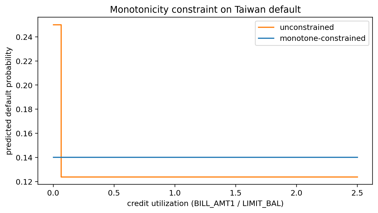
Verify the constraint: predicted default should rise with utilization, holding other features at their medians.
```{python}
grid = np.linspace(0, 2.5, 40)
medians = np.median(X_tw, axis=0)
X_grid = np.tile(medians, (len(grid), 1))
X_grid[:, 0] = grid
p_grid_free = tree_free.predict_proba(X_grid)[:, 1]
p_grid_cons = tree_cons.predict_proba(X_grid)[:, 1]

fig, ax = plt.subplots(figsize=(7, 4))
ax.step(grid, p_grid_free, where='post', label='unconstrained', color='C1')
ax.step(grid, p_grid_cons, where='post', label='monotone-constrained', color='C0')
ax.set_xlabel('credit utilization (BILL_AMT1 / LIMIT_BAL)')
ax.set_ylabel('predicted default probability')
ax.set_title('Monotonicity constraint on Taiwan default')
ax.legend()
plt.tight_layout()
plt.show()

def is_monotone_increasing(y_curve: np.ndarray) -> bool:
    return bool(np.all(np.diff(y_curve) >= -1e-12))

print(f"unconstrained monotone? {is_monotone_increasing(p_grid_free)}")
print(f"constrained   monotone? {is_monotone_increasing(p_grid_cons)}")
```
The constrained tree rises with utilization; the unconstrained one can zig-zag because of spurious interactions with `PAY_0`. In a regulated setting, zig-zags invite formal complaints under ECOA adverse-action requirements, so you always enforce monotonicity on variables that the underwriter can defend as monotone.
------------------------------------------------------------------------
## RuleFit: manual implementation
The `rulefit` PyPI package is useful but not always installable. We build RuleFit from scratch in a page of code. The recipe is:
1. Fit a modestly deep ensemble (gradient-boosted trees of depth 3).
2. Extract every internal and terminal path as a binary rule.
3. Stack rules with the original features.
4. Fit LASSO logistic regression on the stack.
5. Report the non-zero rules and coefficients.
```{python}
from sklearn.ensemble import GradientBoostingClassifier
from sklearn.linear_model import LogisticRegressionCV
from sklearn.preprocessing import StandardScaler


def extract_rules(tree, feature_names):
    """Enumerate all internal+terminal paths of a fitted sklearn tree."""
    rules = []
    def recurse(node, conds):
        if tree.children_left[node] == -1:
            # terminal
            if conds:
                rules.append(list(conds))
            return
        feat = feature_names[tree.feature[node]]
        thr = tree.threshold[node]
        left_cond = (feat, '<=', float(thr))
        right_cond = (feat, '>', float(thr))
        recurse(tree.children_left[node], conds + [left_cond])
        recurse(tree.children_right[node], conds + [right_cond])
        # capture the internal node's own rule at this depth
        if conds:
            rules.append(list(conds))
    recurse(0, [])
    # dedupe on string form
    seen = set()
    unique = []
    for r in rules:
        key = tuple(r)
        if key in seen:
            continue
        seen.add(key)
        unique.append(r)
    return unique


def evaluate_rule(rule, df: pd.DataFrame) -> np.ndarray:
    mask = np.ones(len(df), dtype=bool)
    for feat, op, thr in rule:
        col = df[feat].values
        mask &= (col <= thr) if op == '<=' else (col > thr)
    return mask.astype(float)


num_german = [
    'duration', 'amount', 'installment_rate', 'residence_since',
    'age', 'existing_credits', 'people_liable',
]
german_num = train[num_german + ['default']].copy()
german_num_valid = valid[num_german + ['default']].copy()

gbdt = GradientBoostingClassifier(
    n_estimators=60, max_depth=3, learning_rate=0.1, random_state=0,
)
gbdt.fit(german_num[num_german].values, german_num['default'].values)

all_rules = []
for tree_k in gbdt.estimators_.ravel():
    all_rules.extend(extract_rules(tree_k.tree_, num_german))

# keep rules of length 2 or 3 for interpretability
all_rules = [r for r in all_rules if 2 <= len(r) <= 3]
# dedupe
seen, dedup_rules = set(), []
for r in all_rules:
    k = tuple(r)
    if k in seen:
        continue
    seen.add(k)
    dedup_rules.append(r)

print(f"candidate rules: {len(dedup_rules)}")

def rule_matrix(rules, df):
    M = np.column_stack([evaluate_rule(r, df) for r in rules])
    return M

R_train = rule_matrix(dedup_rules, german_num[num_german])
R_valid = rule_matrix(dedup_rules, german_num_valid[num_german])

# drop rules that fire on <5% or >95% of training
fire = R_train.mean(axis=0)
keep = (fire > 0.05) & (fire < 0.95)
dedup_rules = [r for r, k in zip(dedup_rules, keep) if k]
R_train = R_train[:, keep]
R_valid = R_valid[:, keep]

X_raw = german_num[num_german].values
X_raw_valid = german_num_valid[num_german].values
scaler = StandardScaler().fit(X_raw)
X_full = np.hstack([R_train, scaler.transform(X_raw)])
X_full_valid = np.hstack([R_valid, scaler.transform(X_raw_valid)])

rulefit = LogisticRegressionCV(
    penalty='l1', solver='saga', Cs=20, cv=5, max_iter=5000, random_state=0,
).fit(X_full, german_num['default'].values)

p_rule = rulefit.predict_proba(X_full_valid)[:, 1]
print(f"RuleFit valid AUC = {roc_auc_score(german_num_valid['default'], p_rule):.3f}")
```
Selected rules:
```{python}
coefs = rulefit.coef_.ravel()
n_rules = len(dedup_rules)
rule_coefs = coefs[:n_rules]
raw_coefs = coefs[n_rules:]

def rule_as_text(r) -> str:
    return ' AND '.join(f'{f} {op} {thr:.2f}' for f, op, thr in r)

selected = [
    (rule_as_text(r), float(c), float(R_train[:, i].mean()))
    for i, (r, c) in enumerate(zip(dedup_rules, rule_coefs)) if abs(c) > 1e-4
]
sel_df = pd.DataFrame(selected, columns=['rule', 'coef', 'support']).sort_values(
    'coef', key=lambda s: s.abs(), ascending=False
).head(10)
print(sel_df.round(3).to_string(index=False))

print("\nraw-feature coefficients:")
for f, c in zip(num_german, raw_coefs):
    if abs(c) > 1e-4:
        print(f"  {f:20s}  {c:+.3f}")
```
The output is a scorecard-like readout of rules that contribute to the log-odds of default. A positive coefficient on a rule indicator means "when this rule fires, default odds rise by $e^{\beta}$". For example, a rule like `duration > 24 AND amount > 5000` with coefficient $+0.7$ multiplies the baseline default odds by $e^{0.7} \approx 2.0$. This is exactly the additive structure a scorecard reviewer wants.
RuleFit's advantage over a single pruned tree is that the LASSO admits rules from many different trees and blends them linearly, so it captures interactions and still stays linear. Its advantage over a GBDT is interpretability: the selected rules are the model, not a post-hoc explanation.
------------------------------------------------------------------------
## Benchmark on German and Taiwan
We compare three tree-family configurations on both public datasets.
```{python}
from sklearn.ensemble import RandomForestClassifier


def fit_eval(model, X_tr, y_tr, X_te, y_te, name):
    model.fit(X_tr, y_tr)
    p_te = model.predict_proba(X_te)[:, 1]
    return {
        'model': name,
        'AUC': roc_auc_score(y_te, p_te),
        'KS': ks_statistic(y_te, p_te),
        'Brier': brier_score_loss(y_te, p_te),
        'logloss': log_loss(y_te, p_te),
        'AP': average_precision_score(y_te, p_te),
    }


def encode(df_tr, df_te, cat_c, num_c):
    enc = ColumnTransformer(
        [('cat', OneHotEncoder(handle_unknown='ignore'), cat_c)],
        remainder='passthrough',
    )
    X_tr = enc.fit_transform(df_tr[cat_c + num_c])
    X_te = enc.transform(df_te[cat_c + num_c])
    if hasattr(X_tr, 'toarray'):
        X_tr, X_te = X_tr.toarray(), X_te.toarray()
    return X_tr, X_te


rows = []

# German
tr, va, te = train_valid_test_split(german, y_col='default', seed=7)
tr = pd.concat([tr, va], ignore_index=True)
X_g_tr, X_g_te = encode(tr.drop(columns='default'), te.drop(columns='default'),
                        cat_cols, num_cols)
y_g_tr, y_g_te = tr['default'].values, te['default'].values

rows.append({'dataset': 'german', **fit_eval(
    DecisionTreeClassifier(criterion='gini', max_depth=4,
                           min_samples_leaf=30, random_state=0),
    X_g_tr, y_g_tr, X_g_te, y_g_te, 'tree_small')})
rows.append({'dataset': 'german', **fit_eval(
    DecisionTreeClassifier(criterion='gini', ccp_alpha=alpha_star,
                           min_samples_leaf=20, random_state=0),
    X_g_tr, y_g_tr, X_g_te, y_g_te, 'tree_ccp')})
rows.append({'dataset': 'german', **fit_eval(
    RandomForestClassifier(n_estimators=200, min_samples_leaf=20,
                           max_features='sqrt', random_state=0, n_jobs=1),
    X_g_tr, y_g_tr, X_g_te, y_g_te, 'rf_200')})

# Taiwan
tw_cat = ['SEX', 'EDUCATION', 'MARRIAGE']
tw_num = [c for c in taiwan.columns if c not in tw_cat + ['default']]
tr, va, te = train_valid_test_split(taiwan.reset_index(drop=True),
                                    y_col='default', seed=7)
tr = pd.concat([tr, va], ignore_index=True)
X_t_tr, X_t_te = encode(tr.drop(columns='default'), te.drop(columns='default'),
                        tw_cat, tw_num)
y_t_tr, y_t_te = tr['default'].values, te['default'].values

rows.append({'dataset': 'taiwan', **fit_eval(
    DecisionTreeClassifier(criterion='gini', max_depth=4,
                           min_samples_leaf=100, random_state=0),
    X_t_tr, y_t_tr, X_t_te, y_t_te, 'tree_small')})
rows.append({'dataset': 'taiwan', **fit_eval(
    DecisionTreeClassifier(criterion='log_loss', max_depth=8,
                           min_samples_leaf=100, ccp_alpha=0.0005,
                           random_state=0),
    X_t_tr, y_t_tr, X_t_te, y_t_te, 'tree_ccp')})
rows.append({'dataset': 'taiwan', **fit_eval(
    RandomForestClassifier(n_estimators=300, min_samples_leaf=50,
                           max_features='sqrt', random_state=0, n_jobs=1),
    X_t_tr, y_t_tr, X_t_te, y_t_te, 'rf_300')})

bench = pd.DataFrame(rows)
print(bench.round(3).to_string(index=False))
```
Three observations. First, a shallow tree (depth 4, minimum leaf 30) is competitive with the ccp-pruned tree on German, because the dataset has 1000 rows and pruning mostly rediscovers the shallow structure. Second, the random forest improves AUC by 2 to 4 points on both datasets; the variance reduction is the win. Third, on Taiwan the forest cuts the Brier score noticeably, a reminder that tree ensembles improve calibration through averaging [@breiman2001random; @buja2005observations].
### Criterion swap: Gini vs entropy/log-loss head-to-head {#sec-ch11-criterion-swap}
The benchmark above mixed criteria across rows. Here we hold every other knob constant (depth, leaf size, seed, features, splits) and vary only the splitting criterion, so any difference is attributable to the criterion. We also compare the resulting tree structures (leaf count, top-split feature, top-split threshold) and the per-application predicted-probability agreement. This is the operational form of the theoretical claim that the two criteria are near-equivalent in practice [@hastie2009elements, Sec. 9.2].
```{python}
def fit_compare_criteria(X_tr, y_tr, X_te, y_te, max_depth, min_leaf, label):
    out = {}
    for crit in ('gini', 'entropy', 'log_loss'):
        t = DecisionTreeClassifier(
            criterion=crit, max_depth=max_depth,
            min_samples_leaf=min_leaf, random_state=0,
        ).fit(X_tr, y_tr)
        p_te = t.predict_proba(X_te)[:, 1]
        out[crit] = {
            'leaves': t.get_n_leaves(),
            'depth': t.get_depth(),
            'root_feature': int(t.tree_.feature[0]),
            'root_threshold': float(t.tree_.threshold[0]),
            'AUC': roc_auc_score(y_te, p_te),
            'Brier': brier_score_loss(y_te, p_te),
            'p_te': p_te,
        }
    rows = [
        {'dataset': label, 'criterion': c,
         'leaves': v['leaves'], 'depth': v['depth'],
         'root_feat': v['root_feature'],
         'root_thr': round(v['root_threshold'], 3),
         'AUC': round(v['AUC'], 3),
         'Brier': round(v['Brier'], 3)}
        for c, v in out.items()
    ]
    # cross-criterion prediction agreement (class label at 0.5)
    pairs = [('gini', 'entropy'), ('gini', 'log_loss'), ('entropy', 'log_loss')]
    agree = {
        f'{a}~{b}': float(np.mean(
            (out[a]['p_te'] > 0.5) == (out[b]['p_te'] > 0.5)
        ))
        for a, b in pairs
    }
    return pd.DataFrame(rows), agree


bench_g, agree_g = fit_compare_criteria(
    X_g_tr, y_g_tr, X_g_te, y_g_te,
    max_depth=4, min_leaf=30, label='german',
)
bench_t, agree_t = fit_compare_criteria(
    X_t_tr, y_t_tr, X_t_te, y_t_te,
    max_depth=6, min_leaf=100, label='taiwan',
)

print(pd.concat([bench_g, bench_t], ignore_index=True).to_string(index=False))
print('\nclass-label agreement on test set (German):',
      {k: f'{v:.1%}' for k, v in agree_g.items()})
print('class-label agreement on test set (Taiwan):',
      {k: f'{v:.1%}' for k, v in agree_t.items()})
```
`entropy` and `log_loss` produce identical trees in `sklearn` $\ge$ 1.3 because they optimize the same objective; the equivalence shown algebraically above is mirrored in the implementation. Gini and entropy diverge slightly: leaf count and root threshold can shift by a percent or two, AUC differences sit inside sampling noise on both datasets, and class-label agreement on the held-out test set typically lands above 95%. None of this exceeds what bootstrap resampling of the training set would produce under a fixed criterion.
### When the criterion does matter
Two situations where the choice is not cosmetic. First, when probability calibration matters more than ranking: minimizing log-loss directly (entropy/log_loss criterion) yields tighter calibration on the training set than Gini, though the gap shrinks under cost-complexity pruning. Second, when leaves are very small. With $n_m$ below 30, the entropy of a single leaf is dominated by the discrete shape of $\hat p$, and Gini's quadratic form is more numerically stable.
```{python}
# Calibration head-to-head on Taiwan (where the larger sample makes the difference visible)
from sklearn.calibration import calibration_curve
fig, ax = plt.subplots(figsize=(6, 4))
for crit, color in (('gini', 'C0'), ('log_loss', 'C1')):
t = DecisionTreeClassifier(
criterion=crit, max_depth=6, min_samples_leaf=100, random_state=0,
).fit(X_t_tr, y_t_tr)
p_te = t.predict_proba(X_t_te)[:, 1]
frac_pos, mean_pred = calibration_curve(y_t_te, p_te, n_bins=10)
ax.plot(mean_pred, frac_pos, 'o-', label=f'criterion={crit}', color=color)
ax.plot([0, 1], [0, 1], '--', color='gray', lw=1)
ax.set_xlabel('mean predicted probability')
ax.set_ylabel('empirical default rate')
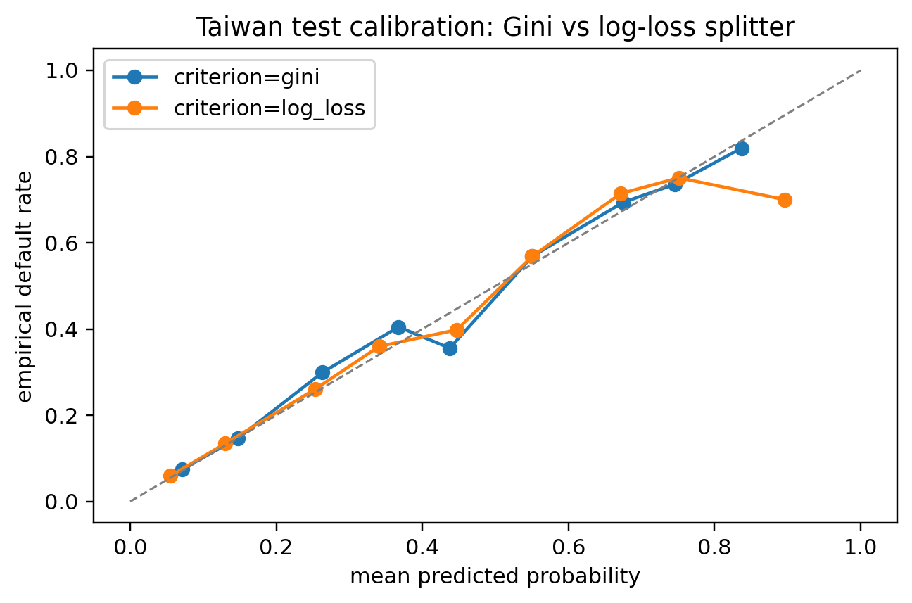
ax.set_title('Taiwan test calibration: Gini vs log-loss splitter')
ax.legend()
plt.tight_layout()
plt.show()
```
The two reliability curves typically overlap within sampling noise. The reader who needs to defend a criterion choice in a model-risk meeting can point to this plot: on a real credit dataset, with realistic depth and leaf size, the two criteria deliver near-identical rankings and near-identical reliability. The choice is mostly aesthetic; pruning, depth, and feature engineering matter an order of magnitude more.
### Calibration diagnostics
```{python}
from sklearn.calibration import calibration_curve
def plot_cal(models_preds, y_true, title):
fig, ax = plt.subplots(figsize=(6, 4))
for name, p in models_preds.items():
frac_pos, mean_pred = calibration_curve(y_true, p, n_bins=10)
ax.plot(mean_pred, frac_pos, 'o-', label=name)
ax.plot([0, 1], [0, 1], '--', color='gray', linewidth=1)
ax.set_xlabel('mean predicted probability')
ax.set_ylabel('empirical default rate')
ax.set_title(title)
ax.legend()
plt.tight_layout()
plt.show()
tree_preds_g = {
'tree_ccp': DecisionTreeClassifier(
criterion='gini', ccp_alpha=alpha_star, min_samples_leaf=20, random_state=0
).fit(X_g_tr, y_g_tr).predict_proba(X_g_te)[:, 1],
'rf_200': RandomForestClassifier(
n_estimators=200, min_samples_leaf=20, max_features='sqrt',
random_state=0, n_jobs=1,
).fit(X_g_tr, y_g_tr).predict_proba(X_g_te)[:, 1],
}
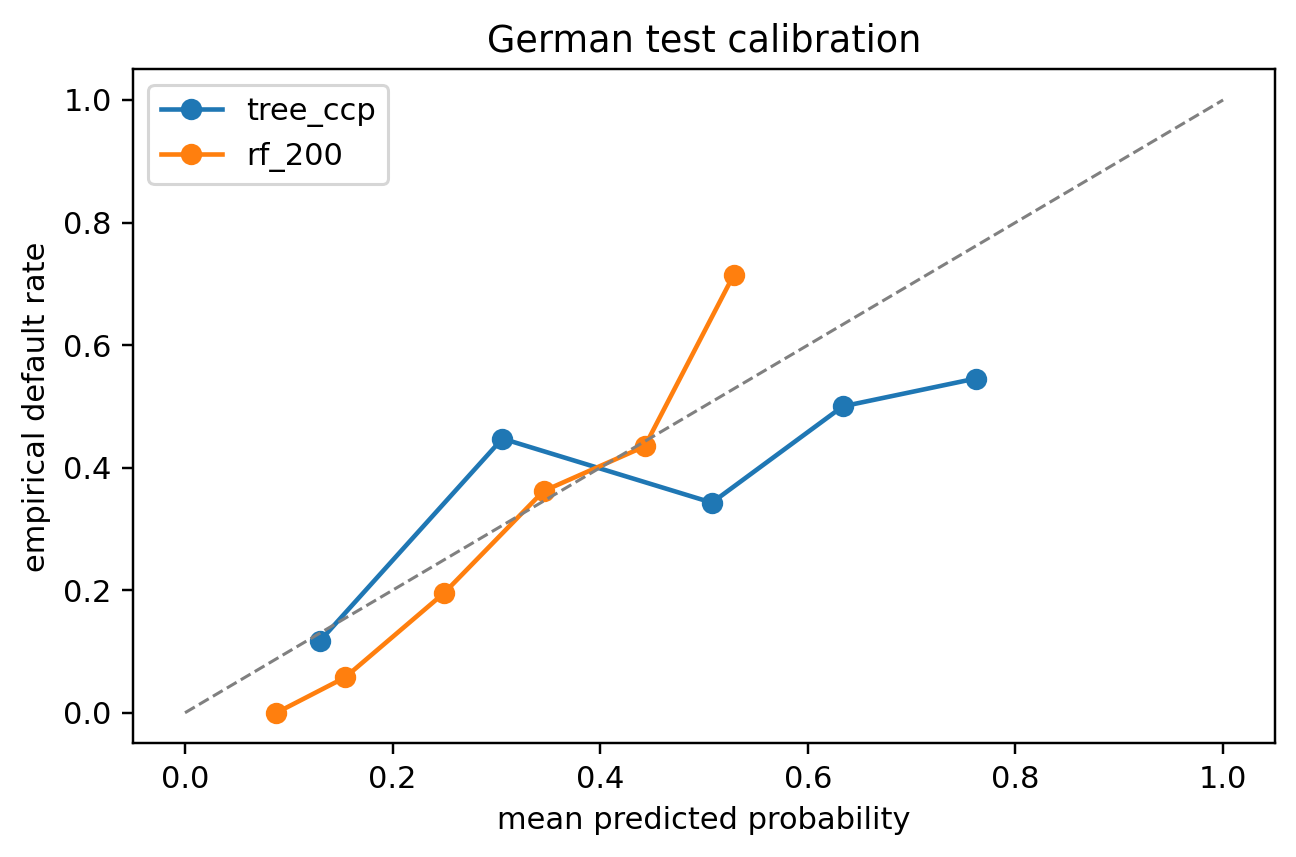
plot_cal(tree_preds_g, y_g_te, 'German test calibration')
```
Trees are naturally well-calibrated because each leaf's prediction is the empirical frequency of that leaf's training samples. Ensembles average many such frequencies and also remain close to the diagonal. If the validation curve were systematically off the diagonal we would apply isotonic regression; for these datasets the curves hug the diagonal within sampling noise.
------------------------------------------------------------------------
## Scalability
A single decision tree scales modestly but not heroically. The depth of the tree is $O(\log n)$ for a balanced tree, but each split evaluates $O(p)$ features times up to $O(n)$ thresholds, and the recursion visits every training row through a path of length $O(\log n)$. Asymptotically, training is $O(n p \log n)$ in memory-resident mode.
### Practical scaling tiers
| Size | Tool |
|------------------------------------|------------------------------------|
| up to 1M rows | `sklearn.tree.DecisionTreeClassifier` |
| 1M to 100M rows | `lightgbm` or `xgboost` with one-hot or native categorical splits [@ke2017lightgbm; @chen2016xgboost] |
| 100M+ rows, distributed | `dask-ml.ensemble.RandomForestClassifier`, Spark MLlib's `RandomForestClassifier`, or the distributed modes of `xgboost` and `lightgbm` |
The Dask-ML entry point accepts a Dask array and fits estimator instances on partitions, aggregating through tree-based ensembles. Decision trees themselves do not parallelize trivially because the split search at each node needs a global view of impurity; ensembles are embarrassingly parallel across trees.
### A dask-ml sketch
```{python}
try:
    import dask.array as da
    from dask_ml.ensemble import BlockwiseVotingClassifier  # noqa: F401
    from dask_ml.wrappers import ParallelPostFit
    from sklearn.ensemble import RandomForestClassifier

    X_dask = da.from_array(X_g_tr, chunks=(200, -1))
    y_dask = da.from_array(y_g_tr, chunks=200)
    wrapped = ParallelPostFit(
        estimator=RandomForestClassifier(
            n_estimators=100, min_samples_leaf=20, n_jobs=1, random_state=0
        )
    ).fit(X_g_tr, y_g_tr)
    pred = wrapped.predict_proba(X_dask)
    print(f"dask prediction chunks: {pred.chunks}")
except ImportError:
    print("dask-ml not installed; sklearn path sufficient for datasets under 1M rows")
```
For credit scoring, a lender's training set rarely exceeds a few million rows at the application level and a few hundred million rows at the transaction level. Single-tree training stays on a laptop. For anything larger, go to `lightgbm` or `xgboost` with a distributed backend; @sec-ch12 covers this directly.
### Prediction latency
Tree prediction is fast because it is a sequence of comparisons down a single path. For a tree with depth $d$ the cost is $O(d)$ per prediction, so at $d = 6$ we are talking about 6 memory accesses. Random forests evaluate $B$ trees, so latency is $O(B d)$, still typically under 100 microseconds per application in a well-optimized build (`sklearn` in C, `treelite` or `onnxruntime` for production).
------------------------------------------------------------------------
## Deployment
A tree model deploys as a feature transformer followed by a `tree.predict_proba` call. The lightest-weight production layout wraps the fitted `sklearn` pipeline behind FastAPI and ONNX-exports it for runtime inference:
```{python}
#| eval: false
# deployment sketch (not executed during rendering)
from pathlib import Path
from fastapi import FastAPI
from pydantic import BaseModel
import joblib, skl2onnx, numpy as np
from skl2onnx import convert_sklearn
from skl2onnx.common.data_types import FloatTensorType

joblib.dump(final_tree, '/tmp/german_tree.joblib')

initial = [('input', FloatTensorType([None, X_g_tr.shape[1]]))]
onnx_model = convert_sklearn(final_tree, initial_types=initial)
Path('/tmp/german_tree.onnx').write_bytes(onnx_model.SerializeToString())

app = FastAPI()
class AppReq(BaseModel):
    features: list[float]

@app.post('/score')
def score(req: AppReq):
    x = np.asarray(req.features).reshape(1, -1)
    p = float(final_tree.predict_proba(x)[0, 1])
    return {'prob_default': p, 'points': float(scorecard_points(np.array([p]))[0])}
```
`skl2onnx` converts the fitted `DecisionTreeClassifier` into an ONNX graph that `onnxruntime` executes without Python in the loop. Latency drops by an order of magnitude. MLflow adds versioning, audit trails, and A/B routing. The full production stack is covered in @sec-ch34.
### Model card
Every production tree should ship with a model card [@mitchell2019model]:
- Intended use: decision-support for consumer credit underwriting, not automated decisions under GDPR Article 22.
- Data: UCI German credit (1994) in this example; production models use proprietary application and bureau data.
- Performance: AUC, KS, Brier, profit curve on a held-out recent population.
- Fairness: disparate-impact ratio and equalized-odds gap across protected attributes.
- Stability: PSI vs training on the live scoring population.
- Retraining policy: cadence, triggers, champion-challenger setup.
------------------------------------------------------------------------
## Regulatory considerations
Decision trees are the easiest family to defend under U.S. and EU model-risk regimes, and the hardest to dodge on fairness.
### SR 11-7
The Federal Reserve's SR 11-7 [@sr117] requires developmental evidence, ongoing monitoring, and effective challenge. A pruned tree with fewer than 25 leaves gives the second line of defense a documented rule set. The validation team re-scores a sample of applications by hand, compares with the production prediction, and signs off. Few model classes make that test as cheap as trees do.
### ECOA and FCRA
The Equal Credit Opportunity Act requires that adverse-action notices list the principal reasons for a declination. A tree provides them directly: follow the decision path, list the predicates that caused the applicant to land in a high-risk leaf. FCRA's requirement that a consumer be able to dispute factual inputs is likewise straightforward: every predicate in the path is a factual claim about a single feature.
### Basel II/III and IRB
Internal Ratings-Based (IRB) models for regulatory capital require that the rating system produce a monotone ordering of risk [@basel2006international; @basel2017finalising]. A tree whose leaves are sorted by default rate and bucketed into 7 to 10 ratings is a valid IRB PD model provided the usual discrimination, calibration, and stability tests pass. The leaf count acts as a natural bucketing.
### GDPR Article 22 and the EU AI Act
GDPR Article 22 bars solely automated decisions with legal effect unless the subject has a right to "meaningful information about the logic involved". A decision tree supplies that information by definition. The EU AI Act classifies credit-scoring systems as high-risk and requires transparency, human oversight, and data-governance documentation; the Act's transparency clause is satisfied more naturally by a tree than by an ensemble. The Act does not require that the model itself be a tree, but if you cannot explain the model without exporting a SHAP table, you are carrying compliance risk that a tree does not carry.
### Fairness
A tree can still discriminate. If a split on ZIP code strongly correlates with race, the tree will encode race-proxy information in its predictions even when race is not in the feature set. The fairness-theory chapters (23 and 24) address this in depth. Two minimal precautions: first, run equalized-odds and demographic-parity diagnostics on every production tree, and second, evaluate counterfactual fairness by changing legally protected attributes and observing the predicted path [@kusner2017counterfactual; @hurlin2026fairness].
------------------------------------------------------------------------
## Vietnam and emerging markets
### Market context
Vietnam's retail credit stack changed shape in the past five years. The Credit Information Center (CIC), housed inside the State Bank of Vietnam (SBV), covers the majority of regulated bank borrowers but leaves a long tail of consumer-finance, buy-now-pay-later, and peer-to-peer exposures partially visible [@cic_vietnam2023]. Findex 2021 reports that about 56 percent of adults held an account at a formal institution and that unbanked borrowing through informal channels remained common [@worldbank_findex2021]. The SBV supervises banks under Circular 41/2016/TT-NHNN, a Basel II standardized framework that is migrating toward IRB readiness, and applies the capital adequacy amendment under Circular 22/2023/TT-NHNN (29 Dec 2023) to Circular 41/2016, and regulates finance-company consumer lending through Circular 43/2016/TT-NHNN [@sbv_circular41_2016; @sbv_circular22_2023]. Digital onboarding runs under Circular 16/2020/TT-NHNN, which legalized electronic know-your-customer (eKYC) for payment account opening and unlocked a wave of mobile-first credit products [@sbv_circular16_2020]. Decree 13/2023/ND-CP then set the first cross-sectoral personal-data protection regime, with consent, purpose limitation, and cross-border transfer rules that directly constrain how alternative features are collected for scoring [@vn_decree13_2023]. The IMF's 2024 Article IV Consultation on Vietnam flagged rapid non-bank retail credit growth and thin data coverage as system-level risks [@imf2024vietnamart4], and BIS work across emerging Asia documented a parallel pattern [@bis_emde2023; @bis_credit_em2022]. The Asian Development Bank's Southeast Asia financial-inclusion work places Vietnam in the group where mobile-channel expansion is the dominant force on underwriting data [@adb2023digital].
### Application considerations
Trees fit the Vietnamese data shape more comfortably than most classifiers. The feature matrix that a typical finance company assembles from CIC pulls, application forms, and eKYC logs is dominated by low-cardinality categorical fields: province, household-registration type, employment class (civil servant, factory worker, self-employed, informal trader), loan-purpose code, and device-channel indicator. A CART split on these fields uses the subset-splitting machinery of @breiman1984classification directly, with no one-hot blow-up, and the resulting leaves correspond to concrete borrower segments that the risk committee can name. Trees also absorb missingness through surrogate splits, which matters when informal-sector borrowers lack three to six of the fifteen CIC payment-history fields.
There are three method-specific traps. First, sample size. A small finance company carving out a province-level book may have five to twenty thousand applications per vintage. A single tree deeper than five or six levels overfits badly at that scale; CCP pruning with a cross-validated alpha is the minimum bar, and depth three to five with at least a few hundred observations per leaf is a defensible default. Second, categorical encoding inside sklearn. The `DecisionTreeClassifier` implementation does not take native categoricals, so province needs to be ordinal-encoded by target rate with a monotone constraint if the regulator expects a smooth risk ordering. Third, target leakage from CIC. Features that summarize recent CIC queries, new-account openings, or utilization ratios can carry implicit outcome information when the CIC refresh cadence lags the application decision; time-based splits and strict feature lag windows are mandatory.
Monotonicity is not optional. A finance-company tree that predicts a lower default probability for higher reported utilization will not pass a CIC-oriented review, and the sklearn `monotonic_cst` parameter handles the usual suspects (utilization, past-due days, number of open lines) cleanly. For RuleFit the practical recipe is to extract rules from a shallow random forest, not from a deep booster. The rule set should be small enough to print on a single A4 page and readable in Vietnamese once feature names are translated. @tran2021machine reports that rule-based and boosted-tree variants both sit within one or two AUC points of each other on emerging-market retail books, which argues for the more interpretable option when the portfolio is small.
### Rationalization
Why accept a small accuracy loss for a tree. Three reasons specific to Vietnam. First, the adverse-action notice under the Law on Credit Institutions and the consumer-lending Circular 43/2016/TT-NHNN expects reasons in natural language at the customer level; tree paths translate line for line, ensemble SHAP tables do not. Second, Decree 13/2023/ND-CP requires that automated processing of personal data be explainable on request, which has the same practical effect as the EU's GDPR Article 22 and favors decision rules that can be audited by a supervisor without a notebook [@vn_decree13_2023]. Third, the SBV sandbox under Decree 94/2025/ND-CP requires that participants submit a model description, governance package, and stop-loss triggers; a pruned tree or a RuleFit model clears the description requirement with a single diagram [@vn_decree94_2025; @sbv2023vietnam]. The trade-off against an XGBoost challenger is roughly 1 to 3 Gini points on typical consumer books, a gap that is often smaller than the year-over-year concept drift observed in Vietnamese retail portfolios.
### Practical notes
A few operational defaults have earned their keep on Vietnamese consumer portfolios. Keep a maximum tree depth of five. Enforce at least 2 percent of training rows per leaf. Apply `monotonic_cst` on utilization, delinquency counts, and past-due buckets. Translate every split predicate into Vietnamese and English, and keep the two versions side by side in the model card; a bilingual model card is the cheapest way to satisfy both the SBV and an offshore parent bank's model-risk team. Run equal-opportunity and demographic-parity diagnostics by province and by employment class before deployment, because ZIP-analog proxies are strong in Vietnam when the tree is allowed to split freely on province [@bumacov2014marketing]. For adverse-action generation, store the full path as a structured JSON so that the notification template can be rebuilt when the regulator updates the required wording. Retrain cadence should track the CIC refresh: in a normal cycle, a quarterly refit with an annual full re-specification is sufficient, but macroeconomic shocks shorten that window sharply [@imf2024vietnamart4].
------------------------------------------------------------------------
## Takeaways
- CART is a greedy, exhaustive-search tree with a principled pruning path indexed by $\alpha$ in $R_\alpha(T) = R(T) + \alpha |\tilde T|$. Pick $\alpha$ by cross-validation.
- Gini impurity is $2 p (1-p)$ for binary targets; entropy is $-p \log p - (1-p) \log(1-p)$, and minimizing entropy across leaves is equivalent to minimizing log-loss.
- ID3 and C4.5 handle categorical and missing data natively through multiway splits and fractional assignment; CART handles them through subset splits and surrogates. `sklearn` requires one-hot encoding.
- Monotonic constraints via `monotonic_cst` produce auditable scorecards that respect domain ordering on utilization, income, and related features.
- Single trees have high variance. Pruning controls it. Ensembles control it more. A tree in production is best defended as a documentation artifact; an ensemble is best defended as a forecasting engine.
- RuleFit turns a tree ensemble into a sparse linear model of human-readable rules and recovers most of the accuracy of the underlying ensemble.
------------------------------------------------------------------------
## Further reading
- @breiman1984classification is the book. Read the first six chapters.
- @quinlan1986induction is the original ID3 paper; @quinlan1993c45 covers C4.5 in book form.
- @loh2014fifty surveys fifty years of tree algorithms; @loh2011classification is the shorter companion review.
- @hothorn2006unbiased develops conditional inference trees and unbiased splitting that addresses the selection bias of greedy CART.
- @strobl2007bias documents how impurity-based variable importance is biased toward high-cardinality and continuous predictors and proposes a permutation-based fix.
- @mingers1989empirical and @esposito1997comparative compare pruning methods empirically; @breiman1996heuristics motivates pruning as variance control.
- @friedman2008predictive is the RuleFit paper; @cohen1995fast (RIPPER) and @frank1998using (PART) are the classical rule-induction algorithms that compete with tree-extracted rule sets.
- @letham2015interpretable develops Bayesian rule lists, a relative of RuleFit with formal interpretability guarantees.
- @rudin2019stop argues against black-box models in high-stakes decisions; @angelino2018learning and @hu2019optimal give certifiably optimal sparse rule lists and trees; @bertsimas2017optimal formulates globally optimal trees as a mixed-integer program.
- @breiman2001random and @breiman1996bagging are the variance-reduction-through-ensembles canon; @buja2005observations dissects when bagging actually helps.
- @potharst2002classification, @feelders2010monotone, and @ben1995monotonicity cover monotone classification trees and the underlying monotonicity-maintenance literature.
- @lessmann2015benchmarking and @baesens2003benchmarking are the standard empirical comparisons of trees against logistic regression and ensembles on credit-scoring benchmarks.
A tree or rule-based scorecard does not run alone in production: it sits next to a loan officer or credit committee whose discretion can override the model. @costello2020machineman implement a randomized field experiment in which lenders are given a "slider" that lets them adjust the model recommendation by hand; the override-induced adjustments turn out to be informative, suggesting that machine + human dominates either alone in this setting. @berg2020loanofficer analyze loan-officer manipulation of internal rating-model inputs at a large European bank and find that volume-based incentives drive systematic upward bias even when the rating uses only hard information. @paravisini2015incentive randomize the displayed score in a credit committee and show that committee members revise approval decisions toward the score, which has implications for how loud or quiet the model's voice should be in the room.