---
execute:
echo: true
eval: true
warning: false
---
# Data: Sources, Features, and Preprocessing {#sec-ch03}
::: {.callout-note appearance="simple" icon="false"}
**Scope: both retail and corporate, retail-leaning.** Bureau, application, transaction, and alternative-data sources. Worked examples lean retail (UCI German, Taiwan, CIC Vietnam); corporate financial-statement features are covered alongside.
:::
## Overview {.unnumbered}
Credit scoring lives or dies on its inputs. A logistic model trained on the wrong population, a gradient-boosted tree fit to leaky features, or a deep network that imputes missingness with a mean will all fail in production, and they will fail in ways that regulators care about. The modeling choices that textbooks emphasize matter. The data choices matter more.
This chapter takes data seriously. We walk through the traditional sources that sit inside a bank's scorecard, catalog the alternative signals that have appeared in the past decade, and formalize the preprocessing steps that translate raw tables into model-ready features. Three tools get most of the attention: (1) weight of evidence for monotone encoding, (2) imputation for missingness, and (3) time-aware splitting for leakage control. Each is worked out in math and in code that runs on the public UCI data sets.
The chapter also makes a scalability argument. A scorecard team that only thinks in pandas hits a wall at a few million rows. Polars, Dask, and Spark each solve a different piece of that wall, and weight of evidence encoding is one of the simplest places to show the tradeoff. The last section walks through a classic leakage bug, trains a model on it, and shows the out-of-time hit.
A note for the emerging-market reader. The data stack this chapter describes (bureau file, internal core-banking data, alternative overlays) looks different when the bureau is the Credit Information Center (CIC) rather than Experian, when roughly half the adult population has no tradeline, when declared income comes from cash work rather than payroll, and when the origination channel is a mobile app with an eKYC liveness check rather than a branch visit. The preprocessing decisions that follow, weight-of-evidence binning, missingness treatment, and point-in-time feature construction, have to absorb a higher missingness rate, a shorter tradeline depth, and a heavier reliance on transaction-level cash-flow features. The chapter's methods are the right methods, but the defaults (bin counts, IV thresholds, imputation strategy) need to be set with the thin-file population in mind.
The intended reader is a senior practitioner or an academic researcher who already understands logistic regression and classical statistical learning. The chapter spends no time re-deriving maximum likelihood for a linear model; it spends most of its time on the joins, the cohort definitions, and the pre-model transformations that separate a demonstration notebook from a production scorecard. The empirical sections lean on UCI German and UCI Taiwan because they are reproducible everywhere, but the methods port cleanly to larger Home Credit, LendingClub, and HMDA samples covered in later chapters.
### Notation {.unnumbered}
We use $X \in \mathcal{X}$ for features and $Y \in \{0, 1\}$ for the default label, with $Y = 1$ denoting a bad. Population rates are $\pi_1 = \Pr(Y = 1)$ and $\pi_0 = 1 - \pi_1$. A binned feature partitions $\mathcal{X}$ into disjoint bins $\{A_j\}_{j=1}^{J}$. For a categorical variable, bins are level groupings. For a numeric variable, bins are intervals. Conditional probabilities are $p_{j \mid 1} = \Pr(X \in A_j \mid Y = 1)$ and $p_{j \mid 0} = \Pr(X \in A_j \mid Y = 0)$.
```{python}
#| label: setup-imports
import sys, warnings, time
warnings.filterwarnings("ignore")
sys.path.insert(0, "../code")

import numpy as np
import pandas as pd
import matplotlib.pyplot as plt

from creditutils import load_german_credit, load_taiwan_default, stable_sigmoid

rng = np.random.default_rng(42)
np.random.seed(42)
```
## Traditional data {#sec-ch03-data}
Banks have collected the same categories of consumer credit data for four decades. Little has changed in the core schema. The four pillars of a traditional retail scorecard are the bureau report (@sec-ch03-bureau), the bank's internal master file (@sec-ch03-internal), the application form (@sec-ch03-application), and the external overlay such as income verification or fraud flags (@sec-ch03-overlays).
### The bureau report {#sec-ch03-bureau}
A consumer credit bureau is a private clearinghouse. It ingests monthly tradeline updates from thousands of furnishers, normalizes them into a canonical schema, and sells reports and scores back to lenders. In the United States the three nationwide bureaus are Equifax, Experian, and TransUnion [@avery2003overview]. The Fair Credit Reporting Act (FCRA) governs what they can collect, how long they can keep it, and what consumers can dispute. Europe runs a mix of positive and negative bureaus by country. China operates the Credit Reference Center of the People's Bank of China alongside several private bureaus.
A bureau report breaks into five sections that every modern scorecard touches:
1. **Identification**: name, date of birth, social security or national identifier, current and prior addresses. Used to link the report to the application and to detect identity fraud.
2. **Tradelines**: one row per active or closed credit account. Each tradeline has an opening date, an account type (revolving, installment, mortgage, open), a credit limit or original balance, a current balance, a minimum payment, and a 24-month payment history string such as `OK OK OK 30 60 OK OK ...`. These strings are the raw material for every delinquency-based feature.
3. **Inquiries**: every hard pull in the past two years, with date and subscriber name. A burst of inquiries in the last 30 days is a strong short-horizon risk signal.
4. **Public records**: bankruptcies, tax liens, civil judgments. Post-NCAP changes in the United States, most judgments and tax liens no longer appear, which reshaped the public record feature bank after 2017.
5. **Collections**: charged-off accounts placed with third-party collectors. Often shown with original creditor, collection agency, and charge-off balance.
The FICO score, the dominant consumer credit score in the United States, derives from bureau data only. Myfico.com publishes the category weights: payment history (roughly 35 percent), amounts owed (30 percent), length of credit history (15 percent), new credit (10 percent), credit mix (10 percent). The underlying algorithm is proprietary, but its inputs are public knowledge and follow a small number of archetypes. Utilization is the ratio of revolving balance to limit, computed per tradeline and aggregated to the file level. Delinquency depth is the worst 24-month payment code on each line, rolled up to file level as the fraction of tradelines that were 30+, 60+, or 90+ in the last 6, 12, or 24 months. Age features include the age of the oldest account and the average age of open tradelines.
VantageScore, the joint bureau product, and the proprietary scorecards that large lenders build in-house use the same tradeline and inquiry data but different binning, weighting, and target definitions. A common pattern inside a bank is to stack an in-house behavioral score on top of a bureau score, so the scorecard captures both the generic credit-file signal and the account-specific behavior that the bureau does not see.
The specific feature vocabulary is remarkably stable across bureaus and across decades. A partial list of the archetype features a scorecard developer can expect to find useful:
- `bureau_score`: the FICO or VantageScore on file at the observation date.
- `oldest_tradeline_age_months`: age of the oldest account. Tracks length of credit history.
- `avg_open_tradeline_age_months`: average age of open tradelines. Captures both length and churn.
- `utilization_revolving`: sum of balance divided by sum of limit across open revolving lines.
- `utilization_maximum_tradeline`: the maximum utilization across any single revolving tradeline.
- `num_tradelines_30dpd_12m`: count of tradelines that reached 30+ days past due in the last 12 months.
- `num_tradelines_60dpd_24m`: the 60+ DPD analog over 24 months.
- `num_inquiries_6m`: hard pulls in the last 6 months.
- `num_new_tradelines_12m`: newly opened accounts in the last 12 months.
- `bankruptcy_flag`, `collections_flag`, `tax_lien_flag`: public record presence indicators.
- `secured_installment_flag`, `mortgage_flag`: structural presence indicators.
- `revolving_total_balance`, `installment_total_balance`: dollar aggregates by account type.
- `months_since_last_delinquency`: recency of the most recent bad event; "never" is usually coded as a large positive number.
A clean scorecard typically uses 15 to 30 of these, with roughly a two-thirds weight on delinquency-adjacent features (past behavior), a 15-percent weight on utilization (current behavior), and a 10- to 20-percent weight on length and mix (structural).
### Bank internal data {#sec-ch03-internal}
Internal data is what the lender knows from its own books. It is almost always more predictive than bureau data for customers who already hold a product. A current-account issuer sees the full flow of salary credits and direct debits. A mortgage servicer sees escrow behavior. A credit card issuer sees transactional authorizations in real time.
The operational data stores used for model building tend to be organized by the source system:
- **Core banking**: account master, balances, interest accruals, statement-level tables.
- **Card authorization**: every swipe, with merchant category, amount, timestamp, and channel.
- **Payments and transfers**: ACH, wire, SEPA, faster payments, internal transfers.
- **Collections**: arrears, promise-to-pay history, agent notes, settlement agreements.
- **Customer contact**: call center records, digital channel logs, complaint flags.
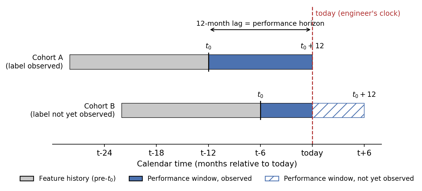
A behavioral scorecard reduces this to a set of standardized windows: 1-month, 3-month, 6-month, and 12-month. Each window is aggregated into counts, sums, max, min, ratios, and trends. A typical card model will have 30 to 80 such features. The specific recipe matters less than the window discipline. The windows must end strictly before the observation point of the score, and they must be computable at that same point in the production path. If they are not, the model is leaky, a topic we return to in @sec-ch03-temporal-leakage-and-lookahead-bias.
There is a structural asymmetry between new-account origination scorecards and behavioral scorecards on existing accounts. An origination scorecard knows the bureau, the application, and nothing else. A behavioral scorecard on an existing card account has the full payment, balance, and transaction history of that account, along with the bureau refresh. The behavioral scorecard is almost always more accurate within its existing customer base; it typically reaches Gini coefficients in the 0.55 to 0.70 range on 12-month horizons, while origination models for the same lender reach 0.40 to 0.55. The gap comes entirely from the richer internal data.
Two specific internal features consistently dominate in behavioral scorecards. The first is the ratio of payment to statement balance, also called the revolving-pay rate. A customer who pays the full balance every month is structurally lower risk than one who pays the minimum, even at the same utilization. The second is the trend in transaction frequency and amount over the last 3 to 6 months. A sudden drop in transaction count while balance grows is a strong short-horizon risk signal, often preceding a 30+ DPD event.
### Account-level versus customer-level modeling
Some scorecards are built per-account; others are built per-customer. The choice matters. A customer-level model aggregates across all of the customer's accounts with the lender and produces one score. An account-level model produces a score per account, so a customer with three cards receives three scores. The customer-level model is more data-efficient but forces the aggregation to happen before the model sees the data. The account-level model is more flexible but requires the lender to manage three predictions for the same person.
In practice, origination uses the customer level (one application, one decision) and account management uses the account level (per-card credit-line changes, per-card repricing). IFRS 9 and CECL (@sec-ch35) have specific implications: the expected credit loss calculation is at the account level, so account-level PDs are the operational requirement even when the decision model runs at the customer level.
### Application data {#sec-ch03-application}
The application form is the scorecard's only chance to see information a customer volunteers that is not in the bureau or the internal master file. Typical fields are employment status, occupation, income, employer tenure, housing tenure, marital status, dependents, purpose of loan, requested amount, and term. Most fields are self-reported. Some lenders cross-check a subset through payroll data providers or open-banking connections.
Application features are high-signal for thin-file borrowers, who by definition have sparse bureau records. For customers with thick files, the marginal value of application data is lower, and the scorecard usually regresses toward bureau features. Income is the perennial exception. A consistent, verified income feature dominates many other inputs, even for thick-file customers.
### Tradeline-level features
The bureau delivers tradelines as a repeated-measures structure. A report with 12 open tradelines contains 12 rows of account-level information, not 1 aggregated row. Turning that into a single observation per borrower is a feature engineering problem, and it is where most scorecard teams spend their time.
Three families of aggregation dominate:
1. **Pointwise**: count of open installments, sum of revolving balances, and maximum utilization.
2. **Temporal**: count of tradelines with 30+ delinquency in the last 12 months, months since last delinquency, months since the oldest account opened.
3. **Structural**: presence of mortgage, presence of auto loan, ratio of secured to unsecured balance.
Modern gradient-boosted scorecards work directly on 100 to 500 such derived columns. Classical scorecards collapse further to 15 to 30 features, selected by information value and stability. We build both kinds in @sec-ch07 and @sec-ch12; this chapter sets up the ingredients.
Tradeline aggregation is where many hidden failure modes live. A common one is double-counting: if a mortgage is reported by both the servicer and the originator for a brief window, a naive aggregation double-counts it in the mortgage-count feature and in the sum-of-balances feature. Bureaus use identifier keys to deduplicate, but the keys are imperfect, and lenders usually write their own dedupe rules. Another is the treatment of authorized users: a thin-file consumer can ride on a spouse's or parent's revolving account, and the bureau reports the authorized user tradeline in the primary report. Whether the feature engine counts that line is a policy choice that affects both risk discrimination and fair lending posture.
### The credit-invisible and unscored populations
A large fraction of adults in any jurisdiction have insufficient bureau data to produce a score. @brevoort2016credit estimate that roughly 26 million Americans are credit invisible, meaning they have no bureau record, and another 19 million are unscored, meaning their record exists but is too thin or stale for the bureau's scoring model. The invisible and unscored populations skew younger, non-white, and lower-income, which makes them the principal policy target for alternative-data scoring. Any scorecard designed for mass-market retail lending has to make an explicit choice about how to treat thin-file applicants. The three common choices are (1) to score them on a dedicated thin-file model, (2) to route them to a judgmental underwriter, or (3) to decline by default. Each choice has fair-lending implications that model governance must document.
### External overlays {#sec-ch03-overlays}
A bureau report is not the only external data source. Income verification services like The Work Number, Finicity, and Plaid provide real-time payroll feeds that confirm stated income within seconds. Fraud databases such as FICO's Falcon, LexisNexis ThreatMetrix, and Early Warning Services flag known fraud rings, synthetic identities, and device fingerprints. AML and sanctions screening, while not directly part of credit risk, feeds the same decision workflow, and its data quality affects the stability of any model downstream. Model governance treats each overlay as a separate data source requiring its own lineage documentation, its own monitoring, and its own retraining plan.
## Alternative data
The line between "traditional" and "alternative" is time-dependent. Utility payment data was alternative in 2005 and is standard today. What the term currently means is any signal that is not in a nationwide credit bureau and not in a bank's own ledger. Five categories cover most of what large lenders have deployed or piloted.
### A working taxonomy
1. **Psychometric**: survey-style questionnaires designed to measure personality traits (conscientiousness, honesty, locus of control) that correlate with repayment. Deployed in frontier markets where bureau coverage is sparse.
2. **Behavioral and device**: smartphone metadata, browser fingerprints, typing dynamics, session-level app usage. @berg2020rise document that ten easily observed digital footprint variables, such as device operating system and time-of-day login patterns, deliver predictive power comparable to a credit bureau score at a German e-commerce lender.
3. **Transactional**: bank account data obtained through open banking APIs (PSD2 in Europe, CDR in Australia, the 1033 rule in the United States). Each transaction has a date, amount, counterparty, and a classification tag.
4. **Social and platform**: data collected inside a digital platform. @iyer2016screening and @lin2013judging show that in peer-to-peer lending, social ties and soft information embedded in listings contain residual risk information beyond traditional hard information.
5. **Utility and telco**: electricity, water, mobile phone bills. Thin-file consumers often have 6 to 24 months of telecom usage even when they have zero tradelines.
Chinese BigTech platforms have reported that transactional and platform data dominate bureau data for their own ecosystem [@bis2020data; @gambacorta2024data]. The underlying point is older than FinTech. The richer the lender's view of the borrower's cash flow, the less a centralized bureau adds on the margin.
### The information content of alternative data
For any new feature, the relevant question is whether it adds risk-adjusted discrimination on top of what the scorecard already has. @berg2020rise formalize this through nested models, regressing default on credit bureau score alone, on digital footprint alone, and on both. The marginal $R^2$ from adding digital footprints is comparable to the marginal $R^2$ of the bureau score itself. @gambacorta2024data run a similar test using Chinese fintech data and show that a model built on transactional data alone beats a model built on a bureau score alone, although the two together beat either.
The regulatory question, which we will see in @sec-ch05, is whether the resulting model complies with fair lending rules. Alternative data that correlates with protected characteristics can open disparate impact exposure even when the feature is nominally neutral. The empirical finding in @fuster2022predictably is that machine learning models with richer feature sets can widen or narrow racial pricing gaps depending on the choice of input set. Data policy is a model policy.
### Pitfalls of alternative data
Alternative data has three recurring failure modes. First, many signals drift fast. A social feature built in 2015 might not exist in 2025 because the platform has changed. Second, the distribution of missingness is usually not random. A customer without a smartphone has no device fingerprint, and the absence correlates with both income and credit risk. Third, the population on which an alternative data model is validated is almost always a self-selected sample of borrowers who consented to the data collection. Reject inference, covered in @sec-ch10, becomes essential.
A fourth, less-discussed failure mode is the regulatory half-life of novelty. When a signal first enters the market, it usually carries strong predictive power and light compliance scrutiny. As it diffuses across lenders, the signal loses economic rent, adversarial actors learn to game it, and regulators begin to ask how it maps onto protected classes. @fuster2022predictably make the latter point sharply for ML scorecards: models with richer feature sets can move the distribution of predictions in ways that widen or narrow racial pricing gaps, and the direction is not determined by the model class alone. Data governance for alternative signals needs an explicit sunset clause in the same way that a model governance framework has a model retirement clause.
### Cash flow underwriting
Cash flow underwriting is the most important new category of alternative data in the past five years. The workflow starts with a consumer-consented open-banking pull of 12 to 24 months of transaction history across all of the customer's depository accounts. A categorizer assigns each transaction a merchant category and a cash-flow tag (inflow, fixed outflow, discretionary outflow, transfer, fee). Aggregate features are computed at daily, weekly, and monthly frequency: net cash flow, income stability, rent coverage ratio, recurring debit presence, and overdraft count. @bis2020data argue that the informational content of this data can substitute for collateral in SME lending, which is a strong statement about its power.
Two operational facts make cash-flow underwriting different from the other alternative categories. It is consented, so the data subject is aware of the collection in a way that is rarely true for device or behavioral features. And it is structured, so the feature engineering pipeline can be specified and tested deterministically. These properties make cash flow data easier to defend in model validation. They also constrain the universe: only applicants who connect a bank account have any signal at all, which maps directly back onto the missingness-at-design problem that structural alternative data creates.
### Summary of marginal information content
Across the empirical literature, the pattern is consistent. A credit bureau score captures roughly two-thirds of the variation in default that the combined set of bureau, bank, and alternative data captures, with the remaining third split roughly evenly across application data (for thin-file) and alternative data (for both thin- and thick-file). The size of the alternative data contribution depends strongly on the customer segment. For prime thick-file borrowers, the alternative signal is mostly redundant. For thin-file, credit-invisible, and frontier-market borrowers, the bureau is sparse, and the alternative signal is essential. This heterogeneity argues for a segmented modeling approach rather than a single global model. Later chapter treat inclusion and segmentation head-on.
## Weight of evidence and information value {#sec-ch03-weight-of-evidence-and-information-value}
### Why bin features at all?
Before any formula, it is worth asking why a credit team would throw away information by replacing a continuous income figure with the bucket it falls into. The answer is that binning exchanges resolution for six properties that matter more than resolution in the production setting where a scorecard runs for years against drifting data and is subject to formal model validation.
1. **Robustness to outliers, measurement error, and reporting noise.** Bureau fields are reported with varying conventions across furnishers; income is self-reported on applications and has long upper tails; tradeline counts are zero-inflated. Bins absorb all of this into a discrete level whose log-odds contribution is bounded.
2. **Explicit treatment of missingness.** A missing tradeline summary is not the same as a zero. Binning makes the missing level its own bin with its own WoE, so the model uses missingness as a signal when it is informative and ignores it when it is not. No imputation choice is hidden inside the pipeline.
3. **Monotone, additive contribution to log-odds.** WoE-encoded features enter the logistic regression as linear terms whose coefficients factor cleanly into a base-odds piece and a per-bin contribution (@eq-logit-woe), which is what enables the points-based scorecard formulation in @sec-ch07. Underwriters and adverse-action systems can read each bin's contribution as a fixed point increment.
4. **Stability across resamples and through time.** A coarse five-bin partition of a feature is far more stable under resampling and population drift than a continuous coefficient, because the only thing that can change is the per-bin event rate. A scorecard that is refreshed annually but whose binning was set during development needs the binning to be stable across years; that is what the bootstrap and through-time diagnostics in the stability subsection below test.
5. **Two-stage decoupling of binning and coefficient estimation.** Bin selection is supervised but happens before the model is fit. The binning table is reviewed in isolation against IV, monotonicity, and bin-share rules. The coefficient estimation step then becomes essentially a sanity check, because the slope on a single WoE-encoded feature is approximately $-1$ in population. This decoupling is what lets a five-person scorecard team ship a model that a ten-person model risk team can validate.
6. **A model artifact that regulators read.** SR 11-7 model risk validators, ECOA Reg B examiners reviewing reason codes, and GDPR Article 22 explainability reviewers all expect a tabular artifact that lists every model input, every bin, and every contribution. The binning table *is* that artifact. No post-hoc explanation method (SHAP, LIME, permutation importance) produces something that validators trust the same way, because those methods are computed on the trained model rather than fixed at training time.
The first three reasons are the technical ones taught in @siddiqi2017intelligent. The last three are the institutional reasons that explain why binned-WoE pipelines remain dominant in retail credit even decades after gradient boosting matched or exceeded their predictive performance. We return to the question of whether modern algorithms eliminate the need for any of this in the subsection on modern models below.
Weight of evidence (WoE) is the canonical encoding used for this purpose in credit, going back to Kullback's work on information statistics in the 1950s [@kullback1951information] and commercialized in banking by Fair, Isaac, and Company in the 1970s. @siddiqi2017intelligent is the industry-standard reference for the practical pipeline.
### Formal definition
Fix a feature that has been binned into $J$ disjoint bins $A_1, \dots, A_J$. For each bin define the share of goods and share of bads that fall in that bin:
$$
g_j = \frac{\#\{i: x_i \in A_j, y_i = 0\}}{\#\{i: y_i = 0\}},
\qquad
b_j = \frac{\#\{i: x_i \in A_j, y_i = 1\}}{\#\{i: y_i = 1\}}.
$$ {#eq-shares}
The weight of evidence for bin $j$ is the log-ratio of those shares:
$$
\mathrm{WoE}_j = \ln\!\left(\frac{g_j}{b_j}\right).
$$ {#eq-woe}
Positive WoE means the bin is enriched with goods relative to the base rate. Negative WoE means the bin is enriched with bads. The information value of the feature is the weighted sum
$$
\mathrm{IV} = \sum_{j=1}^{J} (g_j - b_j) \mathrm{WoE}_j = \sum_{j=1}^{J} (g_j - b_j) \ln\!\left(\frac{g_j}{b_j}\right).
$$ {#eq-iv}
Practitioners rank features by IV with the rules of thumb from @siddiqi2017intelligent: IV less than 0.02 is unpredictive, 0.02 to 0.1 is weak, 0.1 to 0.3 is medium, 0.3 to 0.5 is strong, and above 0.5 is suspiciously good and usually means the bin count is too fine or the feature is leaky.
### A worked example by hand
Before invoking `optbinning`, it helps to compute the formulas in @eq-shares and @eq-iv on a toy portfolio with three bins. Suppose 1,000 applicants split across an `income_bucket` feature with $G = 900$ goods and $B = 100$ bads in total:
```{python}
#| label: woe-by-hand
import numpy as np, pandas as pd

ex = pd.DataFrame({
    "bin":   ["Low", "Mid", "High"],
    "goods": [250, 370, 280],
    "bads":  [ 50,  30,  20],
})
G, B = ex["goods"].sum(), ex["bads"].sum()
ex["g_j"]   = ex["goods"] / G
ex["b_j"]   = ex["bads"]  / B
ex["WoE_j"] = np.log(ex["g_j"] / ex["b_j"])
ex["IV_j"]  = (ex["g_j"] - ex["b_j"]) * ex["WoE_j"]
print(ex.round(4).to_string(index=False))
print(f"\nIV (total) = {ex['IV_j'].sum():.4f}")
```
Read the table row by row. The Low bin holds $250/900 \approx 27.8\%$ of all goods but $50/100 = 50\%$ of all bads. Its WoE is $\ln(0.278/0.500) \approx -0.59$, a negative value flagging higher-than-average risk, consistent with a $50/300 = 16.7\%$ bad rate against the population base rate of $10\%$. The High bin reverses the imbalance and contributes $\mathrm{WoE} \approx +0.44$. The IV total of about $0.21$ would land the feature in the "medium predictive" tier of the rule of thumb above.
Three sanity checks the table makes obvious:
- The columns $g_j$ and $b_j$ each sum to $1$, because they are class-conditional shares.
- A bin with $g_j = b_j$ contributes zero to IV, because $\ln(1) = 0$. Equality in every bin is exactly the case where the feature is independent of $Y$.
- Both negative and positive WoE bins contribute positively to IV, because the signs of $(g_j - b_j)$ and $\mathrm{WoE}_j$ always match.
These same numbers are what `optbinning` would print if it were given the same three bins, modulo the Laplace pseudo-count discussed in the from-scratch implementation below.
### Equivalence to a symmetric KL divergence
The IV in @eq-iv is exactly the symmetrized Kullback-Leibler divergence between the class-conditional distributions of the binned feature. Let $P$ denote the distribution of $X$ conditional on $Y = 0$ and $Q$ the distribution of $X$ conditional on $Y = 1$, so $P(A_j) = g_j$ and $Q(A_j) = b_j$. The KL divergence of $P$ from $Q$ is
$$
D_{\mathrm{KL}}(P \parallel Q) = \sum_j g_j \ln(g_j/b_j).
$$ {#eq-kl-pq}
By symmetry,
$$
D_{\mathrm{KL}}(Q \parallel P) = \sum_j b_j \ln(b_j/g_j) = -\sum_j b_j \ln(g_j/b_j).
$$ {#eq-kl-qp}
Adding the two,
$$
D_{\mathrm{KL}}(P \parallel Q) + D_{\mathrm{KL}}(Q \parallel P)
= \sum_j (g_j - b_j)\ln(g_j/b_j)
= \mathrm{IV}.
$$ {#eq-iv-eq-kl}
Information value is the Jeffreys divergence between the good and bad class-conditional feature distributions [@kullback1951information]. Two consequences follow:
1. IV is always non-negative, with equality if and only if $g_j = b_j$ for all $j$, the case where the feature contains no information about the label.
2. IV is additive across independent disjoint features only in the limit where no feature carries any information contained in another, so the IV-based ranking should be read as a marginal screen, not a joint optimum.
### Connection to logistic regression
The link to logistic regression is tight. Conditional on bin $j$,
$$
\mathrm{logit} \Pr(Y = 1 \mid X \in A_j)
= \ln\!\left(\frac{\Pr(Y=1, X \in A_j)}{\Pr(Y=0, X \in A_j)}\right)
= \ln\!\left(\frac{\pi_1}{\pi_0}\right) + \ln\!\left(\frac{b_j}{g_j}\right)
= \alpha - \mathrm{WoE}_j,
$$ {#eq-logit-woe}
where $\alpha = \ln(\pi_1 / \pi_0)$ is the log base-odds. Fitting a logistic regression on a single WoE-encoded feature recovers an intercept equal to $\alpha$ and a slope equal to $-1$ in population. In sample, the slope is close to $-1$ and the deviation measures how close the bin assignment is to the saturated model. Because of @eq-logit-woe, WoE encoding gives logistic regression coefficients that factor cleanly into a base-odds piece and a bin-contribution piece, which is what enables the standard points-based scorecard formulation we develop in @sec-ch07.
### Empirical ranking on Taiwan default
```{python}
#| label: iv-ranking-taiwan
from optbinning import BinningProcess
from sklearn.model_selection import train_test_split

df_tw = load_taiwan_default().drop(columns=["id"])
y_tw = df_tw["default"].astype(int).values
X_tw = df_tw.drop(columns=["default"])

X_tr, X_te, y_tr, y_te = train_test_split(
    X_tw, y_tw, test_size=0.3, random_state=42, stratify=y_tw
)

bp = BinningProcess(variable_names=X_tw.columns.tolist())
bp.fit(X_tr.values, y_tr)

iv_tbl = (bp.summary()
          .loc[:, ["name", "iv", "js", "gini", "n_bins"]]
          .sort_values("iv", ascending=False)
          .reset_index(drop=True))
iv_tbl.head(15).round(4)
```
`optbinning` [@navas2020optimal] uses a mixed-integer programming formulation to find an optimal monotone binning that maximizes IV subject to monotonicity and bin-size constraints. The algorithm extends classical supervised discretization [@fayyad1993multi] by enforcing risk monotonicity, which is what underwriters expect from a scorecard. The highest-IV feature in the Taiwan data is the most recent delinquency code (`PAY_0`), followed by older payment codes, which matches the domain intuition.
The `summary()` table includes two additional ranking columns alongside `iv`, both computed on the same binned distributions and sometimes preferred when IV is unstable.
- **`js`: Jensen-Shannon divergence.** A bounded, symmetric variant of the KL divergences from @eq-kl-pq and @eq-kl-qp. With $M = (P + Q)/2$ the bin-share midpoint, $\mathrm{JS}(P, Q) = \tfrac{1}{2} D_{\mathrm{KL}}(P \parallel M) + \tfrac{1}{2} D_{\mathrm{KL}}(Q \parallel M)$. Always lies in $[0, \ln 2]$, so it cannot blow up the way IV can when a bin is nearly empty. Read the same way as IV: bigger means more class separation. Often used as a robustness check on the IV ranking.
- **`gini`: bin-level Gini coefficient.** Twice the area between the bin-ordered cumulative-goods and cumulative-bads curves; equivalently $2 \cdot \mathrm{AUC} - 1$ computed using the bin-ordered WoE as the score. Reported on $[0, 1]$. Same monotone direction as IV but scaled like the discriminative AUC measure used in @sec-ch04, so it lets the scorecard team compare a feature's marginal predictive contribution against the overall model AUC in the same units. The full treatment of AUC, Gini, KS, and Brier sits in @sec-ch04.
In practice, these three columns rank features almost identically; large disagreements are a flag that one bin is dominating IV, in which case a coarser binning or a JS-based ranking is the safer choice.
### WoE-encoded features versus raw features in logistic regression
```{python}
#| label: woe-vs-raw-logreg
from sklearn.linear_model import LogisticRegression
from sklearn.preprocessing import StandardScaler
from sklearn.metrics import roc_auc_score

X_tr_woe = bp.transform(X_tr.values, metric="woe")
X_te_woe = bp.transform(X_te.values, metric="woe")

lr_woe = LogisticRegression(max_iter=1000, C=1.0).fit(X_tr_woe, y_tr)
auc_woe = roc_auc_score(y_te, lr_woe.predict_proba(X_te_woe)[:, 1])

scaler = StandardScaler()
X_tr_raw = scaler.fit_transform(X_tr.values)
X_te_raw = scaler.transform(X_te.values)
lr_raw = LogisticRegression(max_iter=1000, C=1.0).fit(X_tr_raw, y_tr)
auc_raw = roc_auc_score(y_te, lr_raw.predict_proba(X_te_raw)[:, 1])

pd.DataFrame({
    "encoding": ["WoE", "raw (standardized)"],
    "AUC": [auc_woe, auc_raw],
}).round(4)
```
The WoE-encoded logistic model gains roughly 4 to 5 AUC points relative to standardized raw features on Taiwan. The gap narrows once we move to flexible models like gradient boosting, which can internally approximate monotone step functions. The gap persists, however, for the class of linear models that regulators prefer because they are auditable.
Three mechanisms drive the gap, and naming them clarifies when WoE will help and when it will not.
1. **Linearization in log-odds.** WoE turns a non-monotone or kinked empirical risk curve into a monotone, additive contribution in log-odds space, exactly the space the logistic link operates in. A single linear coefficient then fits a relationship that the raw feature would need a polynomial, spline, or piecewise basis to express.
2. **Common units across columns.** WoE rescales every feature, numeric or categorical, into log-odds. The L2 penalty in `LogisticRegression` therefore stops privileging high-variance columns over high-information ones, which is what causes the standardized-raw baseline to leak coefficient mass to noisy features.
3. **Bounded leverage.** Outliers and missing values are absorbed into bins with finite WoE, so a single extreme observation cannot tilt the regression line. Standardization shifts and scales but leaves the long tail intact, and a logistic regression with a few extreme rows still gets dragged.
None of the three is unique to WoE. Splines, target encoders, and isotonic transforms each capture some subset. WoE is the only encoding that captures all three *and* preserves a binning table that a model validator can read. That second property is what makes it the default in regulated retail credit, even where it does not maximize AUC.
### WoE is univariate: handling interactions and non-linearity
WoE is computed one feature at a time, and the IV in @eq-iv treats each feature in isolation. The encoding captures non-linearity *within* a feature (e.g., the bin shape can be U-shaped, monotone, or step), but it does not capture any signal that lives only in the joint distribution of two or more columns. "High credit limit is risky only when paired with a thin payment history" is invisible to a WoE-plus-logistic model unless the interaction is engineered explicitly. Equivalently, the IV-based ranking is a marginal screen: a feature with low IV may still carry conditional information that a joint model would use, and a feature with high IV may be redundant given another already in the model.
This is the structural reason for the AUC gap pattern in the comparison above and in the end-to-end benchmark in @sec-ch03-benchmark. Three remedies sit on a complexity-versus-interpretability spectrum.
1. **Hand-built interaction features.** Cross-tabulate two binned features into a single categorical (`PAY_0` × `LIMIT_BAL_bin`), then WoE-encode the cross. The result stays inside the scorecard pipeline and remains auditable. Cost: combinatorial explosion if used liberally, and small bin counts that hurt stability.
2. **Two-dimensional supervised binning.** `optbinning` ships an `OptimalBinning2D` that solves the same MIP over a pair of features. Useful for a small number of known-interactive pairs (utilization × age of oldest tradeline is a classic).
3. **Segmented scorecards.** Fit one scorecard per pre-defined segment (thin-file vs thick-file, secured vs unsecured). Interactions with the segmenting variable are absorbed by the segmentation. @sec-ch31 treats this in depth.
If the dominant signal is genuinely interactive, none of the above competes with a tree ensemble that splits in arbitrary feature combinations by construction. The empirical fact that WoE-plus-logistic stays close to gradient boosting on regulated retail credit data is a statement about that data: monotone main effects from delinquency, utilization, and tenure dominate, and interactions are second-order, not a general property of the encoding. On data where interactions are first-order (fraud, marketing response on heterogeneous customer pools), the calculus reverses and a tree ensemble is the right starting point.
### A from-scratch implementation
It is good practice to verify the library against a short NumPy reference. The function below reproduces `optbinning`'s per-bin WoE for a fixed set of bin edges.
```{python}
#| label: woe-from-scratch
def woe_iv_from_bins(x: np.ndarray, y: np.ndarray, edges: np.ndarray,
                     laplace: float = 0.5):
    """Return (woe_per_bin, iv, bin_index_of_x) for a fixed set of edges."""
    bin_idx = np.digitize(x, edges[1:-1], right=False)
    df = pd.DataFrame({"bin": bin_idx, "y": y})
    tab = (df.groupby("bin")["y"]
             .agg(["count", "sum"])
             .rename(columns={"count": "n", "sum": "b"}))
    tab["g"] = tab["n"] - tab["b"]
    total_b = max(tab["b"].sum(), 1.0)
    total_g = max(tab["g"].sum(), 1.0)
    p_b = (tab["b"] + laplace) / (total_b + laplace * len(tab))
    p_g = (tab["g"] + laplace) / (total_g + laplace * len(tab))
    woe = np.log(p_g / p_b)
    iv = float(((p_g - p_b) * woe).sum())
    return woe.to_dict(), iv, bin_idx

opt_var = bp.get_binned_variable("LIMIT_BAL")
lib_edges = np.concatenate([[-np.inf], opt_var.splits, [np.inf]])
woe_scratch, iv_scratch, _ = woe_iv_from_bins(
    X_tr["LIMIT_BAL"].values, y_tr, lib_edges
)
iv_lib = float(opt_var.binning_table.build().loc["Totals", "IV"])
print(f"IV (optbinning):  {iv_lib:.4f}")
print(f"IV (from-scratch): {iv_scratch:.4f}")
```
The two IV numbers (here $0.2002$ from `optbinning` and $0.1998$ from the scratch implementation) differ by about $4 \times 10^{-4}$, with the scratch value the smaller of the two. The gap is not a constant offset: it comes from the Laplace pseudo-count of $0.5$, which shrinks the empirical bin shares toward uniform, compresses the WoE magnitudes, and therefore lowers the IV. Setting `laplace=0` in `woe_iv_from_bins` reproduces `optbinning`'s value exactly whenever no bin is empty, which is the right cross-check to run during development. The pseudo-count earns its keep in production, where a single bin occasionally drops to zero in a refresh sample and an unsmoothed $\ln(0)$ would crash the scoring service.
### Reading a binning table
```{python}
#| label: binning-table-example
opt_var.binning_table.build().round(4)
```
This table is the canonical artifact a scorecard developer hands over for model validation. Each row is a bin. The columns show the bin boundaries, the fraction of the population in the bin, the event rate, the WoE, and the IV contribution. The totals row at the bottom gives the IV for the feature. Binning tables like this one are what SR 11-7 [@sr117] validators will read first when reviewing a scorecard submission.
Three diagnostics in the binning table carry most of the validation signal. First, the WoE column should be monotone when the feature is ordinal and the business logic calls for monotonicity. An income feature that increases in WoE, then dips for the highest bin, then increases again, either has too many bins, has a sample-size problem, or has a real structural break (high earners with complicated tax situations, for instance) that needs a dedicated flag. Second, the bin-share column (often labeled `count (%)`) should not have any bin with less than 3 to 5 percent of the population. Small bins have unstable WoE and produce scorecards that swing wildly under resampling. Third, the event rate column should step smoothly across bins when ordered by WoE. Large jumps suggest that the bin boundaries are not where the risk boundary actually sits.
The `optbinning` algorithm is a mixed-integer programming formulation that enforces these properties globally rather than through heuristic post-processing [@navas2020optimal]. It extends the classical supervised discretization literature, which treats binning as a greedy information-gain split, by adding constraints that express what a scorecard developer would actually want. The classical reference is @fayyad1993multi, which uses a minimum description length principle to choose the number of bins. The MIP formulation subsumes this as a special case with different constraints.
### Edge cases in WoE encoding
Three edge cases appear in almost every scorecard build, and each has a standard fix.
**Zero-count bins.** A bin may contain no goods or no bads in the training sample. The raw WoE in @eq-woe is then $\ln 0$ or $-\infty$. Three fixes exist:
1. A Laplace smoothing term adds a pseudo-count of $0.5$ or $1$ to each bin.
2. A bin merge folds the offending bin into an adjacent bin with consistent risk.
3. An `optbinning` constraint on minimum bin size avoids the zero-count state entirely during fitting.
> The Laplace fix is the simplest and adequate for most production code.
**Out-of-range values at scoring time.** Production data may contain values that fall outside the training-time range. For numeric features, the conventional answer is to extend the outermost bins to $(-\infty, \text{edge}_1]$ and $(\text{edge}_{J-1}, \infty)$, so every value maps to a bin. For categorical features, the analog is to keep a catch-all level that absorbs unseen categories with a WoE set equal to the population-weighted average of the observed levels.
**Missing values.** `optbinning` treats missing values as a separate bin, which is the behavior we want. If the missingness itself is informative, the WoE of the missing bin will be nonzero, and the model will use it. If not, the WoE will be close to zero, and the model ignores it. Either way, the treatment is explicit rather than hidden behind a mean imputation.
### Stability of WoE under resampling
A scorecard is only useful if the bin edges and WoE values are stable. Two diagnostics verify stability: bootstrap resampling and through-time partitioning.
```{python}
#| label: woe-bootstrap
from optbinning import OptimalBinning

x_var = X_tr["PAY_0"].values
y_var = y_tr

boot_iv = []
boot_edges = []
boot_rng = np.random.default_rng(0)
for b in range(25):
    idx = boot_rng.integers(0, len(x_var), size=len(x_var))
    ob = OptimalBinning(name="PAY_0", dtype="numerical", max_n_bins=6)
    ob.fit(x_var[idx], y_var[idx])
    iv_b = float(ob.binning_table.build().loc["Totals", "IV"])
    boot_iv.append(iv_b)
    boot_edges.append(tuple(np.round(ob.splits, 3)))

pd.DataFrame({
    "statistic": ["mean IV", "std IV", "min IV", "max IV"],
    "value":     [np.mean(boot_iv), np.std(boot_iv),
                  np.min(boot_iv), np.max(boot_iv)],
}).round(4)
```
If the bootstrap standard deviation of IV is large relative to the mean, the feature's binning is unstable and the scorecard will be brittle. On the `PAY_0` feature the bootstrap spread is modest, which is the expected picture for a strongly predictive feature. Features that fail bootstrap stability almost always benefit from a coarser binning.
### The relationship to supervised discretization
WoE is one member of a family of supervised discretization methods. @fayyad1993multi introduced the entropy-based minimum description length principle for choosing the number of bins. Chi-merge and ChiSquare-based methods use a test of independence between adjacent bins as the merge criterion. The CART tree, treated at length in @sec-ch11, is a univariate supervised binner when grown as a stump, and its splitting criterion is Gini impurity rather than WoE. All of these methods can be expressed as choices of the split function and the stopping criterion; the `optbinning` MIP formulation lets the user specify both explicitly.
The deep reason WoE dominates in credit is not statistical performance but interpretability. A CART split gives a threshold and a count; WoE gives a threshold, a count, and a log-odds contribution that plugs directly into a points-based scorecard. The transformation from WoE to scorecard points is linear in the log-odds, which @sec-ch07 works out in detail.
### Do modern algorithms still need binning and WoE?
A reasonable reading of the chapter so far is that WoE is a piece of legacy machinery that exists because logistic regression cannot handle non-linearity on its own. Gradient boosting splits at arbitrary thresholds, neural networks learn arbitrary feature transformations, and either approach matches the AUC of a WoE-plus-logistic pipeline on most retail credit data. So why bin?
The honest answer has two parts. The first is that for **predictive performance alone**, you do not need WoE if your downstream model is a tree ensemble or a sufficiently regularized neural network. The end-to-end benchmark in @sec-ch03-benchmark makes this explicit: a gradient-boosted model on raw features matches the WoE-plus-logistic configuration on Taiwan within noise. Tree learners pick their own thresholds, absorb missingness through surrogate splits or dedicated handling, and are insensitive to monotone transforms of inputs. WoE is computationally and statistically wasted on them.
The second part is that **production credit scoring is not a pure prediction problem**. It carries six constraints that WoE-style preprocessing addresses by construction and that modern algorithms address only with extra effort:
- **Reason codes for adverse action notices** under ECOA Reg B and FCRA §1681m must be ordered, stable, and explainable per applicant. A scorecard derives reason codes mechanically from the per-bin WoE contributions; a gradient boosting model derives them from SHAP values, which are post-hoc, sample-dependent, and not always monotone in the underlying feature, even when the feature is supposed to be.
- **Monotonicity constraints** on features such as utilization, delinquency, and tenure are required by both regulators and underwriters. WoE binning enforces monotonicity at the binning step; LightGBM and XGBoost support monotonicity flags but at a real cost in fit, and neural networks need either a Lipschitz architecture or a monotone-by-construction layer such as in @sill1998monotonic.
- **Stability under population drift** is harder to guarantee with continuous splits chosen on a single training sample than with bins reviewed against a stability index. Champion scorecards stay in production five-plus years; champion gradient-boosted models are typically refreshed every quarter.
- **Auditability of the model artifact** by SR 11-7 model risk management groups, by GDPR Article 22 explainability reviewers in the EU, and by a non-technical credit committee. The binning table is the artifact those audiences read. SHAP and partial dependence are explanations *of* the artifact, not the artifact itself.
- **Reproducibility across pipelines.** A binning table can be re-implemented by a different team in a different language with the same WoE values. A gradient-boosted model with a particular set of hyperparameters cannot be reproduced exactly outside the original training pipeline.
- **Sample efficiency for thin-file segments.** Where the relevant subpopulation is small (frontier-market lenders, new-to-credit applicants, niche product lines), a five-bin discretization extracts more reliable signal than a continuous spline that needs many degrees of freedom to fit non-linearity.
The pragmatic stack used by many regulated lenders today is a hybrid. Gradient boosting on raw or lightly engineered features is used for ranking and for the challenger model; a WoE-binned logistic scorecard is used for the production decision model that is actually deployed. The two are reconciled with a calibration step. Where a single model must serve both purposes, the rising option is the **Explainable Boosting Machine** (EBM) of @lou2013accurate and @nori2019interpretml, which fits a generalized additive model with one shape function per feature and optionally one shape function per pairwise interaction. EBMs are essentially a continuous-bin generalization of WoE, with the per-feature shape playing the role of the WoE column and the per-pair shape playing the role of an `OptimalBinning2D` cross. They typically match gradient boosting on AUC while preserving the per-feature artifact regulators expect.
So the short answer to "is this an artifact of logistic regression from decades ago?" is: only the *encoding* is. The underlying constraints (e.g., reason codes, monotonicity, stability, auditability, sample efficiency) are not artifacts of the algorithm; they are properties of the regulatory and operational environment in which credit models live. WoE persists because it satisfies those constraints almost for free, not because anyone is nostalgic for the 1970s.
## Missing data {#sec-ch03-missing}
Every real credit data set has missing values. A bureau-less applicant has no tradelines. An application that skipped an optional field has nulls. An open-banking connection that failed mid-session has a truncated history. How missingness gets handled determines, in practice, whether a model works in production for the tail of the customer base where it matters most.
### Rubin's taxonomy
@rubin1976inference classified missing-data mechanisms into three types. Let $X$ be the complete data, $M$ the missingness indicator matrix, and $X_{\mathrm{obs}}, X_{\mathrm{mis}}$ the observed and missing partitions.
- **MCAR** (missing completely at random): $\Pr(M \mid X) = \Pr(M)$. Missingness is independent of both observed and unobserved data. Rare in practice. The classic example is a random sensor dropout.
- **MAR** (missing at random): $\Pr(M \mid X) = \Pr(M \mid X_{\mathrm{obs}})$. Missingness depends only on observed variables. An income field that is more likely to be blank for younger applicants is MAR, because age is observed. Under MAR, likelihood-based methods such as multiple imputation are unbiased.
- **MNAR** (missing not at random): $\Pr(M \mid X)$ depends on $X_{\mathrm{mis}}$. Missingness depends on the unobserved value itself. High earners who decline to report income are MNAR. Imputation alone cannot recover the full data distribution without assumptions.
@little2019statistical gives the textbook treatment. For scorecard work, the relevant message is that MCAR is a convenient fiction, MAR is often defensible given rich observed data, and MNAR is the state of the world for sensitive fields like income, mortgage balance on outside institutions, or credit applications at competitors.
### Imputation strategies
Five strategies cover most of what a scorecard pipeline needs:
1. **Simple statistic**: replace with the column mean, median, or mode. Fast, unbiased under MCAR, biased otherwise. Collapses variance.
2. **Indicator plus statistic**: add a binary "was missing" column and impute the underlying value. Captures the information in the fact of missingness, which for credit is often predictive on its own.
3. **k-nearest neighbors**: find the $k$ most similar rows under a defined distance, average their values. Works well when the data has strong local structure. Compute scales quadratically with sample size.
4. **Multivariate iterative (MICE)**: model each incomplete feature as a function of the others, iterate to convergence [@vanbuuren2011mice; @white2011multiple]. Scikit-learn's `IterativeImputer` is the Python implementation. Recovers MAR under mild assumptions.
5. **Model-based with native support**: tree learners like XGBoost, LightGBM, and CatBoost natively route missing values to the child node that minimizes loss. For those learners, imputation is a pre-model choice only if you also run a linear benchmark.
For credit scoring, the missing-indicator strategy deserves first-line status. If an applicant failed to fill in an optional field, that refusal often correlates with risk. Losing it by silent mean-imputation is a substantive information loss.
### Simulated experiment on German credit
We take the German credit data, inject missingness under the three mechanisms, and compare five imputation strategies on the downstream AUC of a logistic model.
```{python}
#| label: missing-sim-setup
from sklearn.experimental import enable_iterative_imputer  # noqa: F401
from sklearn.impute import SimpleImputer, KNNImputer, IterativeImputer
from sklearn.linear_model import LogisticRegression
from sklearn.pipeline import Pipeline
from sklearn.preprocessing import StandardScaler
from sklearn.model_selection import train_test_split

rng_miss = np.random.default_rng(0)
df_ger = load_german_credit()
num_cols = ["duration", "amount", "age", "installment_rate",
            "residence_since", "existing_credits", "people_liable"]
X_full = df_ger[num_cols].astype(float).copy()
y_full = df_ger["default"].values


def inject_mcar(X, frac, rng):
    X = X.copy()
    for c in X.columns:
        mask = rng.random(len(X)) < frac
        X.loc[mask, c] = np.nan
    return X


def inject_mar(X, driver, frac, rng):
    X = X.copy()
    thr = X[driver].quantile(0.6)
    for c in [c for c in X.columns if c != driver]:
        p = np.where(X[driver] > thr, frac, frac * 0.2)
        mask = rng.random(len(X)) < p
        X.loc[mask, c] = np.nan
    return X


def inject_mnar(X, frac, rng):
    X = X.copy()
    for c in X.columns:
        thr = X[c].quantile(0.7)
        p = np.where(X[c] > thr, frac, frac * 0.1)
        mask = rng.random(len(X)) < p
        X.loc[mask, c] = np.nan
    return X
```
The MCAR mechanism drops each cell independently with probability 0.2. The MAR mechanism drops a cell with probability 0.4 when `duration` is in the top 40 percent and 0.08 otherwise. The MNAR mechanism drops a cell with probability 0.4 when the cell's own value is in the top 30 percent of its column and 0.04 otherwise. Credit analogs map cleanly: MAR is "applicants with long tenure skip optional fields"; MNAR is "applicants with high balances skip the balance field".
```{python}
#| label: missing-sim-run
from sklearn.metrics import roc_auc_score

def eval_imputer(Xtr, Xte, ytr, yte, imputer):
    pipe = Pipeline([
        ("imp", imputer),
        ("scale", StandardScaler()),
        ("lr", LogisticRegression(max_iter=1000)),
    ])
    pipe.fit(Xtr, ytr)
    p = pipe.predict_proba(Xte)[:, 1]
    return roc_auc_score(yte, p)


mechanisms = {
    "MCAR": lambda X: inject_mcar(X, 0.2, rng_miss),
    "MAR":  lambda X: inject_mar(X, "duration", 0.4, rng_miss),
    "MNAR": lambda X: inject_mnar(X, 0.4, rng_miss),
}

imputers = {
    "mean":       SimpleImputer(strategy="mean"),
    "median":     SimpleImputer(strategy="median"),
    "mean+ind":   SimpleImputer(strategy="mean", add_indicator=True),
    "kNN(5)":     KNNImputer(n_neighbors=5),
    "MICE":       IterativeImputer(max_iter=10, random_state=0),
}

records = []
for mech_name, inject in mechanisms.items():
    Xm = inject(X_full)
    Xtr, Xte, ytr, yte = train_test_split(
        Xm, y_full, test_size=0.3, random_state=0, stratify=y_full
    )
    for imp_name, imp in imputers.items():
        auc = eval_imputer(Xtr, Xte, ytr, yte, imp)
        records.append({"mechanism": mech_name, "imputer": imp_name, "AUC": auc})

res_miss = (pd.DataFrame(records)
            .pivot(index="imputer", columns="mechanism", values="AUC")
            .round(4))
res_miss
```
Two observations. First, no imputer dominates across all three mechanisms, which is the expected result once we understand that each method encodes different assumptions. Under MCAR the mean-plus-indicator strategy leads because the indicator itself is random and the underlying distribution is symmetric. Under MAR, mean or median imputation is competitive because the drivers are observed in the other features. Under MNAR no method recovers the full signal. The second observation is that the differences are small in absolute terms, a few AUC points, but they compound into large differences in expected profit when stacked across features. This is where adding a missingness indicator pays dividends for essentially zero cost.
### When to use which
A practical decision rule for scorecard work:
- **Categorical feature with natural "missing" level**: keep the missing level as its own bin. WoE handles it. This is the default in `optbinning`.
- **Continuous numeric with MAR missingness and rich observed data**: `IterativeImputer` (MICE) with a small number of iterations. Add an indicator if missingness rate exceeds 5 percent.
- **Sparse high-dimensional matrix with MNAR fields**: keep the indicator, impute the value with a median. Do not try to be clever.
- **Tree learner downstream**: do not impute. Pass NaNs through. Compare to imputation only if required by governance.
- **Linear or neural scorecard**: impute explicitly and persist the imputer in the same artifact as the model.
The industry's single largest imputation failure mode is pipeline drift. The training data had a missingness rate of 2 percent for income. The production data has 15 percent, because a downstream upstream vendor changed a default. The imputer silently mean-fills the missing values, and the score concentrates near the population mean. Monitor missingness rates on every feature in production with the same care that you monitor PSI (@sec-ch16).
### What about matrix completion, GAIN, MIWAE, MissForest? {#sec-ch03-sota-imputers}
A reasonable reader will ask why the list above stops at MICE when the imputation literature has moved on to low-rank matrix completion [@mazumder2010softimpute], random-forest imputation [@stekhoven2012missforest], generative-adversarial imputation [@yoon2018gain], deep-latent-variable imputation [@mattei2019miwae], and AutoML-style imputer selection [@jarrett2022hyperimpute]. The answer is not that these methods are bad. They are excluded from the recommended scorecard pipeline for four reasons that all bind at the same time in credit.
First, **low-rank assumptions do not fit credit feature matrices**. Matrix completion methods assume the underlying data matrix is approximately low-rank, which is the right model for collaborative filtering (a few latent taste factors generate every user-item rating) and for image inpainting (smoothness in pixel space). Credit features are a heterogeneous mix of bureau scores, demographics, employment fields, behavioral aggregates, and self-reported items. There is no shared low-dimensional latent factor that generates all of them, and SoftImpute-style nuclear-norm completion silently shrinks toward a basis that has no interpretation. Empirically, low-rank completion is competitive on dense numeric panels (e.g., genomics) and weak on the wide mixed-type tables that scorecards consume.
Second, **the inference-time story is broken or expensive**. A scorecard must score one new applicant in milliseconds. Matrix completion, GAIN, and MIWAE were all designed for the in-sample setting, where you complete a fixed matrix once. Out-of-sample completion for a single new row requires either projection onto a stored basis (matrix completion), a forward pass through a generator trained on potentially stale data (GAIN), or sampling from a learned posterior (MIWAE). Each of these adds a second model to the production path that must itself be versioned, monitored for drift, and validated under SR 11-7. The marginal AUC gain rarely justifies the operational cost.
Third, **the empirical lift on tabular data is small**. Two large published benchmarks of imputation methods on tabular data, @jager2021benchmark and @lemorvan2021whatsgood, both find that median imputation with a missing-indicator column is within one or two AUC points of the best deep imputer on essentially every downstream classification task they test. Where the deep methods win, they win by margins that are smaller than the variance across random seeds. For credit, where the dominant model is a gradient-boosted tree that handles NaN natively (@sec-ch12-xgboost), the practical gain from a sophisticated imputer is close to zero.
Fourth, **governance penalizes opacity**. A bank validator will ask three questions about any imputer: what assumption does it encode, what happens when production missingness drifts, and how would you detect a regression. Median-plus-indicator answers all three in one sentence each. GAN- or VAE-based imputation answers none of them cleanly, and the validator will require a separate model risk file, a champion-challenger setup, and ongoing monitoring of the imputer's own outputs. This burden is real and is why most production scorecards still ship with median-plus-indicator or with a tree learner that ignores the question entirely.
The honest summary is that matrix completion and its deep-learning successors are excellent tools for the problems they were designed for (collaborative filtering, image inpainting, gene-expression panels) and a poor fit for the wide-mixed-type, low-latency, high-governance environment of credit scoring. The gap is not theoretical sophistication; it is fit-for-purpose. A team that wants to experiment with HyperImpute or MissForest as a challenger to the median-plus-indicator champion should do so, but the production default belongs with the simpler tool.
### Multiple imputation and variance inflation
Single imputation, where each missing cell is replaced with one value, systematically understates downstream standard errors. Multiple imputation draws $M$ imputed data sets, fits the model on each, and combines the results using the rules of @rubin1976inference. @vanbuuren2011mice and @white2011multiple treat the methodology in detail. For credit scoring, the pragmatic reality is that $M = 1$ is almost always used. The argument is that scorecard inference is about the predicted probability rather than the coefficient standard errors, and the downstream decisions (approve, decline, price) are robust to the kind of variance inflation that single imputation glosses over. That argument is correct for pure decision-making, but breaks down when the model's coefficients are used in capital calculations under Basel IRB, where the regulator cares about the confidence interval around the PD. Banks that run IRB models generally carry a multiple-imputation pipeline for a subset of critical features, even when single imputation is the default for decision making.
### Imputation and monotonicity
A subtle but important property of any imputer is whether it preserves the monotone risk structure that scorecard binning relies on. Mean imputation breaks monotonicity because the imputed value sits near the middle of the distribution, while the underlying missing-value risk may be at one of the tails. Median imputation has the same problem. An imputation strategy that restores monotonicity is to impute to the value that matches the observed risk of the missing group. Operationally, this means fitting a univariate logistic regression of the label on the feature in the non-missing subsample, then assigning the imputed value so that the predicted log-odds of a missing row equals the empirical log-odds of the missing subset. This is worth the effort when downstream scorecard monotonicity is a constraint, and overkill otherwise.
The construction is short enough to demonstrate in code. We inject MNAR missingness on `duration` (longer-duration applicants are more likely to have the field blank, and longer duration is also riskier), then compare the imputed value chosen by the mean, the median, and the risk-matched rule.
```{python}
#| label: risk-matched-impute
from sklearn.linear_model import LogisticRegression as _LR

rng_rmi = np.random.default_rng(7)
X_rmi = X_full.copy()
thr_d = X_rmi["duration"].quantile(0.6)
p_drop = np.where(X_rmi["duration"] > thr_d, 0.6, 0.05)
miss_mask = rng_rmi.random(len(X_rmi)) < p_drop
X_rmi.loc[miss_mask, "duration"] = np.nan

obs = ~X_rmi["duration"].isna()
x_obs = X_rmi.loc[obs, "duration"].values.reshape(-1, 1)
y_obs = y_full[obs]
y_mis = y_full[~obs]

p_mis = y_mis.mean()
logit_mis = np.log(p_mis / (1 - p_mis))

uni = _LR(penalty=None, max_iter=1000).fit(x_obs, y_obs)
a, b = float(uni.intercept_[0]), float(uni.coef_[0, 0])
x_risk = (logit_mis - a) / b

cmp = pd.DataFrame({
    "strategy": ["mean", "median", "risk-matched"],
    "imputed_value": [
        X_rmi["duration"].mean(),
        X_rmi["duration"].median(),
        x_risk,
    ],
})
cmp["pred_logit_at_imp"] = a + b * cmp["imputed_value"]
cmp["empirical_logit_missing"] = logit_mis
cmp["abs_gap"] = (cmp["pred_logit_at_imp"] - logit_mis).abs()
cmp.round(3)
```
The risk-matched row has `abs_gap` equal to zero by construction. The mean and median rows have a positive gap whose sign tells you which direction the imputer is pulling the missing population: a negative `pred_logit_at_imp` minus `empirical_logit_missing` means mean or median imputation is making the missing rows look safer than they really are, which is exactly the failure mode that breaks monotonicity in the downstream scorecard.
```{python}
#| label: risk-matched-auc
def fill_and_score(value, X_in):
    Xf = X_in.copy()
    Xf["duration"] = Xf["duration"].fillna(value)
    Xtr, Xte, ytr, yte = train_test_split(
        Xf, y_full, test_size=0.3, random_state=0, stratify=y_full
    )
    pipe = Pipeline([("scale", StandardScaler()),
                     ("lr", LogisticRegression(max_iter=1000))])
    pipe.fit(Xtr, ytr)
    return roc_auc_score(yte, pipe.predict_proba(Xte)[:, 1])

aucs = {row.strategy: fill_and_score(row.imputed_value, X_rmi)
        for row in cmp.itertuples()}
pd.Series(aucs, name="AUC").round(4).to_frame()
```
The AUC differences are typically small on a single feature, which matches the broader finding from the simulated experiment above. The point of risk matching is not to win the AUC race; it is to keep the scorecard's monotone risk structure intact when the binning step downstream insists on it. Two further notes. First, the rule generalizes from a single feature to a multivariate setting by replacing the univariate logit with a model that uses all observed features and solving for the imputed value of the missing column at the row's own observed covariates. Second, the rule is a single-imputation device. If you need calibrated standard errors, draw the imputed value from the posterior predictive distribution of the univariate logit instead of using the point estimate, then average across draws using Rubin's rules.
### Missingness indicator interpretation
When a missingness indicator column is added, the logistic coefficient on it has a direct risk interpretation. Let $M_j$ be the indicator that feature $j$ is missing and $X_j^{\text{imp}}$ be the imputed value. The fitted model has the form
$$
\mathrm{logit} \Pr(Y=1 \mid X, M)
= \alpha + \beta_j X_j^{\text{imp}} + \gamma_j M_j + \cdots
$$ {#eq-missing-indicator}
The coefficient $\gamma_j$ measures the risk premium (or discount) associated with the fact of missingness itself, holding the imputed value constant. A positive $\gamma_j$ with a substantial magnitude says that a missing-on-$X_j$ row is riskier than an observed row with the same imputed value, which is direct evidence that the missingness mechanism is MNAR. A near-zero $\gamma_j$ is evidence that the mechanism is plausibly MCAR or MAR.
> Two cautions apply. First, the indicator is colinear with the imputed value if every imputed row shares the same value, which in mean imputation is always the case for a single feature. Regularized logistic regression handles this cleanly; unpenalized logistic regression may show nonfinite standard errors. Second, if two features have correlated missingness (for example, both self-reported income and self-reported employment length are blank for the same applicant), adding both indicators recovers almost all the useful signal but can make the model's bias unstable across resampling. A joint "application-form incomplete" indicator often works better than two separate indicators.
## Feature selection
Scorecards live with more features than they use. A fintech's feature store routinely holds thousands of columns. A deployed model uses 10 to 60. The process of getting from one to the other is feature selection. Four approaches cover almost everything production teams deploy.
### IV filter
The simplest screen is to rank every feature by information value and keep the top $K$, or keep every feature with $\mathrm{IV} \ge 0.02$. This is a univariate filter. It ignores correlations. In a scorecard with 500 candidate features and heavy correlation, it is nevertheless the right first step, because it cuts the search space from 500 to 100 or 50 before any multivariate method runs.
```{python}
#| label: iv-filter-example
iv_filter = iv_tbl[iv_tbl["iv"] >= 0.02].reset_index(drop=True)
print(f"Features with IV >= 0.02: {len(iv_filter)} of {len(iv_tbl)}")
iv_filter.head(10).round(3)
```
On Taiwan most of the 23 numeric features clear the 0.02 threshold. The handful that fall below are demographic fields whose marginal signal is weak once `LIMIT_BAL` and the payment-delinquency block are in the pool. On a raw feature store with thousands of variables, two-thirds typically fall below.
### LASSO
The LASSO [@tibshirani1996regression] adds an $\ell_1$ penalty to the logistic log-likelihood,
$$
\hat\beta(\lambda) = \arg\min_{\beta_0, \beta}
\Big\{ -\tfrac{1}{n}\sum_{i=1}^n \ell_i(\beta_0, \beta)
+ \lambda \sum_{j=1}^{p} |\beta_j| \Big\},
$$ {#eq-lasso}
where $\ell_i$ is the per-observation log-likelihood. For $\lambda$ large, the solution is the null model; for $\lambda = 0$ the solution is ordinary logistic regression. Between those extremes, coefficients enter one at a time as $\lambda$ decreases, which gives the characteristic LASSO path. Features whose coefficients remain at zero across most of the path are dropped. The `glmnet` coordinate-descent algorithm [@friedman2010regularization] is the standard solver.
Three properties make LASSO attractive for scorecard selection. First, it handles correlated features by picking one and shrinking the others, which reduces the collinearity problem that flat logistic regression suffers on WoE-encoded features. Second, the regularization path is cheap to compute, so a team can inspect the entire trajectory rather than committing to a single $\lambda$. Third, the elastic net extension [@zou2005regularization] smooths the all-or-nothing selection into a convex combination with ridge regularization, which is usually the better default in production.
```{python}
#| label: lasso-path
from sklearn.linear_model import LogisticRegression
from sklearn.preprocessing import StandardScaler
from sklearn.model_selection import train_test_split

df_tw = load_taiwan_default().drop(columns=["id"])
y = df_tw["default"].values.astype(int)
X = df_tw.drop(columns=["default"]).values.astype(float)
X_tr, X_te, y_tr, y_te = train_test_split(
    X, y, test_size=0.3, random_state=42, stratify=y
)
sc = StandardScaler().fit(X_tr)
X_tr_s = sc.transform(X_tr)
X_te_s = sc.transform(X_te)

Cs = np.logspace(-3, 1, 25)
feat_names = df_tw.drop(columns=["default"]).columns.tolist()
coefs = np.zeros((len(Cs), X_tr_s.shape[1]))
for i, C in enumerate(Cs):
    m = LogisticRegression(penalty="l1", solver="liblinear",
                           C=C, max_iter=2000)
    m.fit(X_tr_s, y_tr)
    coefs[i] = m.coef_[0]

fig, ax = plt.subplots(figsize=(7, 4.2))
for j in range(coefs.shape[1]):
    ax.plot(Cs, coefs[:, j], lw=1.0)
ax.set_xscale("log")
ax.axhline(0, color="k", lw=0.6)
ax.set_xlabel("Inverse regularization strength C (larger C = weaker penalty)")
ax.set_ylabel("Coefficient")
ax.set_title("LASSO logistic regression path on Taiwan default")
plt.tight_layout()
plt.show()
```
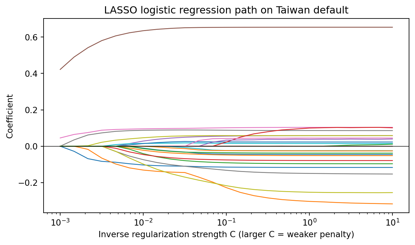
The shape of this plot is typical. At the strongest penalty most coefficients are zero; as the penalty weakens the `PAY_0` family enters first, followed by `LIMIT_BAL` and `PAY_AMT`. When two highly collinear features are present, the LASSO picks one and keeps the other at zero until the penalty is very weak. That behavior is the motivation for the elastic net extension.
```{python}
#| label: lasso-select
C_star = 0.02
m_star = LogisticRegression(penalty="l1", solver="liblinear",
                            C=C_star, max_iter=2000).fit(X_tr_s, y_tr)
kept = np.array(feat_names)[m_star.coef_[0] != 0]
dropped = np.array(feat_names)[m_star.coef_[0] == 0]
print(f"Kept   ({len(kept)}):   {list(kept)}")
print(f"Dropped ({len(dropped)}): {list(dropped)}")
```
At $C = 0.02$, the LASSO drops the weakest features and keeps a compact subset. The practical workflow is to cross-validate over $\lambda$ to pick the operating point, then stability-select across bootstrap resamples to drop features that enter the solution only intermittently.
### Mutual information and permutation importance
Two nonparametric alternatives round out the toolkit.
Mutual information $I(X_j; Y) = \sum_{x,y} p(x,y) \ln \frac{p(x,y)}{p(x)p(y)}$ is closely related to IV. For a binary $Y$, $I(X_j; Y) = H(Y) - H(Y \mid X_j)$, which measures the expected reduction in label entropy from knowing $X_j$. `sklearn.feature_selection.mutual_info_classif` estimates it for continuous and discrete features.
Permutation importance [@breiman2001random; @altmann2010permutation] measures the drop in model performance when a single feature is randomly permuted on the validation set. It is model-agnostic and captures interactions that univariate IV misses. The cost is that permutation importance for correlated features is misleading: permuting one feature often leaves the information intact through its correlated neighbor, so the importance of both looks low. Conditional permutation variants partly fix this.
```{python}
#| label: mi-perm
from sklearn.feature_selection import mutual_info_classif
from sklearn.inspection import permutation_importance

mi = mutual_info_classif(X_tr_s, y_tr, random_state=0)
lr = LogisticRegression(max_iter=1000).fit(X_tr_s, y_tr)
perm = permutation_importance(lr, X_te_s, y_te, n_repeats=10,
                              random_state=0, n_jobs=1)

def conditional_perm_importance(model, X, y, n_repeats=10,
                                corr_thresh=0.5, n_bins=4,
                                random_state=0):
    """Permute each feature within bins of its most-correlated neighbor.

    Approximates Strobl-style conditional permutation: if feature j is
    correlated with k, marginal permutation breaks j but leaves k intact,
    so the model recovers most of the signal and j looks unimportant.
    Permuting j within strata of k removes that leakage path.
    """
    rng = np.random.default_rng(random_state)
    base = model.score(X, y)
    corr = np.abs(np.corrcoef(X, rowvar=False))
    np.fill_diagonal(corr, 0)
    out = np.zeros(X.shape[1])
    for j in range(X.shape[1]):
        partner = int(np.argmax(corr[j]))
        if corr[j, partner] < corr_thresh:
            strata = np.zeros(X.shape[0], dtype=int)
        else:
            strata = pd.qcut(X[:, partner], q=n_bins,
                             labels=False, duplicates="drop")
        drops = np.empty(n_repeats)
        for r in range(n_repeats):
            Xp = X.copy()
            for s in np.unique(strata):
                idx = np.where(strata == s)[0]
                Xp[idx, j] = rng.permutation(Xp[idx, j])
            drops[r] = base - model.score(Xp, y)
        out[j] = drops.mean()
    return out

cond_perm = conditional_perm_importance(lr, X_te_s, y_te,
                                        n_repeats=10, random_state=0)

imp_df = (pd.DataFrame({
            "feature": feat_names,
            "MI": mi,
            "perm_importance": perm.importances_mean,
            "cond_perm_importance": cond_perm,
         })
         .sort_values("MI", ascending=False)
         .reset_index(drop=True))
imp_df.head(10).round(4)
```
The mutual-information ranking and the marginal permutation-importance ranking agree on the top features with the IV ranking, which is the usual picture when the candidate set is clean. When they disagree, disagreement usually points to either collinearity (MI and IV up, permutation importance down) or a nonlinear interaction (permutation importance up, MI down). The conditional permutation column sharpens this read: features whose marginal importance was suppressed by a correlated neighbor recover here, because permuting within strata of that neighbor blocks the leakage path. A feature that looks important marginally but collapses under conditional permutation is mostly proxying for its partner; a feature that looks weak marginally but rises under conditional permutation carries information the rest of the matrix cannot reconstruct.
Reading the table, the top ten are all repayment-status (`PAY_*`) and payment-amount (`PAY_AMT*`) variables, consistent with the IV ranking in @sec-ch03-weight-of-evidence-and-information-value. `PAY_0`, the most recent repayment status, dominates on every column: $I(X;Y) \approx 0.079$, marginal permutation importance $\approx 0.040$, and conditional permutation importance $\approx 0.021$. It is the only feature whose importance survives conditioning, meaning its signal is not reconstructible from any single correlated neighbor.
The older repayment lags tell the collinearity story cleanly. `PAY_2` through `PAY_6` have non-trivial mutual information (roughly $0.03$-$0.05$) but their marginal permutation importance is already near zero, and conditional permutation drives it to zero or slightly negative. Mechanically, `PAY_0` through `PAY_6` are strongly autocorrelated across months, so shuffling `PAY_2` alone barely hurts the model because `PAY_0` (and the other lags) still carry the same delinquency signal. Mutual information is a univariate quantity and does not see this substitution, which is why the MI column stays elevated while both permutation columns collapse. The practical consequence is that the linear model is essentially reading `PAY_0` and using the older lags as noisy confirmation; dropping `PAY_3`-`PAY_6` would barely move held-out performance, though keeping them can still help in nonlinear models that exploit interactions (e.g. "was delinquent two months ago but recovered").
The `PAY_AMT*` variables sit at the bottom of the table with MI around $0.02$ and permutation importance within sampling noise of zero (the small negative values at `n_repeats = 10` are pure variance, not evidence against the feature). For a linear model on the standardized scale, raw payment amounts carry little marginal information once repayment status is known: a customer who is two months delinquent is risky regardless of whether last month's payment was \$500 or \$5,000. These features typically become useful only after transformation (ratio to bill amount, log-scaling) or inside a model that can interact them with `PAY_0`.
### Boruta
Boruta [@kursa2010boruta] is a wrapper method built on random forests. For each feature it creates a shadow feature that is a random permutation of the original. A random forest is fit on the augmented matrix, and each real feature is tested against the best shadow feature. Features that consistently beat their shadow are confirmed; features that lose consistently are rejected; borderline features are marked as tentative. Boruta is aggressive in retaining correlated relevant features, which is desirable when the downstream model can handle them, and it is slow.
```{python}
#| label: boruta-optional
from boruta import BorutaPy
from sklearn.ensemble import RandomForestClassifier

rf = RandomForestClassifier(
    n_estimators=200, max_depth=7, n_jobs=-1,
    class_weight="balanced", random_state=0,
)
boruta = BorutaPy(
    estimator=rf, n_estimators="auto",
    max_iter=50, random_state=0, verbose=0,
)
boruta.fit(X_tr_s.astype(np.float64), y_tr.astype(int))

feat_arr   = np.array(feat_names)
confirmed  = feat_arr[boruta.support_]
tentative  = feat_arr[boruta.support_weak_]
rejected   = feat_arr[~(boruta.support_ | boruta.support_weak_)]

print(f"Confirmed ({len(confirmed)}): {confirmed.tolist()}")
print(f"Tentative ({len(tentative)}): {tentative.tolist()}")
print(f"Rejected  ({len(rejected)}): {rejected.tolist()}")
```
On Taiwan, Boruta confirms a broad core (around nineteen of the twenty-three predictors): `LIMIT_BAL`, every `PAY_*` delinquency counter, every `BILL_AMT_*`, and every `PAY_AMT_*`. The four demographics (`SEX`, `EDUCATION`, `MARRIAGE`, `AGE`) are rejected. This overlaps heavily with the LASSO choice at $C \approx 0.05$ and with the top of the IV ranking: the repayment-history block dominates regardless of which selector we trust.
### Stability across methods
A useful diagnostic is to compare the top-10 features from each method. If three of four methods agree on a feature, it is very likely signal. If a feature appears in only one method, investigate. The literature, going back to @guyon2003introduction, warns against over-reliance on any single score; practical scorecard teams combine a univariate filter (IV), a sparse model (LASSO), and a nonlinear wrapper (Boruta or permutation importance on a tree learner) before freezing the feature list.
### Stability selection
A richer version of the stability argument is stability selection, introduced in the statistics literature for LASSO-type methods. The idea is to fit the LASSO on many bootstrap resamples and record how often each feature is selected. Features that appear in 80 or 90 percent of bootstraps are confirmed; features that appear in fewer than 50 percent are rejected; the intermediate band is marked for review. Stability selection has strong theoretical guarantees for controlling the expected number of false positives in high-dimensional settings.
```{python}
#| label: stability-selection
n_boot = 30
C_sel = 0.05
boot_sel = np.zeros((n_boot, X_tr_s.shape[1]), dtype=int)
boot_rng_s = np.random.default_rng(0)
for b in range(n_boot):
    idx = boot_rng_s.integers(0, len(X_tr_s), size=len(X_tr_s))
    m = LogisticRegression(penalty="l1", solver="liblinear",
                           C=C_sel, max_iter=2000)
    m.fit(X_tr_s[idx], y_tr[idx])
    boot_sel[b] = (m.coef_[0] != 0).astype(int)

selection_freq = boot_sel.mean(axis=0)
stab = (pd.DataFrame({"feature": feat_names,
                      "selection_frequency": selection_freq})
          .sort_values("selection_frequency", ascending=False)
          .reset_index(drop=True))
stab.head(10).round(3)
```
Features that appear in every bootstrap fit are the robust core of the model. Features that appear in 50 to 70 percent of fits are correlated with the robust core and will drop in and out depending on the resample. Features that appear in fewer than 30 percent of fits are weak and should be removed even if they clear the IV threshold.
### Redundancy analysis
Univariate feature selection tells you which features carry signal; it does not tell you which features are redundant. Redundancy analysis uses the correlation structure of the candidate matrix to collapse highly correlated groups before fitting the downstream model.
```{python}
#| label: redundancy-correlation
import numpy as np
corr = np.corrcoef(X_tr_s, rowvar=False)
labels = feat_names

# find pairs with |r| > 0.8 among the kept features
pairs = []
for i in range(len(labels)):
    for j in range(i + 1, len(labels)):
        if abs(corr[i, j]) > 0.8:
            pairs.append((labels[i], labels[j], round(float(corr[i, j]), 3)))
pd.DataFrame(pairs, columns=["feature_a", "feature_b", "correlation"]).head(12)
```
Pairs with absolute correlation above 0.8 are the candidates for group collapse. One common rule is to keep the higher-IV member of each pair and drop the other. Another is to collapse the pair into a ratio or a difference feature that captures the residual signal. For scorecard work, the former is simpler and adequate; for gradient boosting, neither matters because the tree learner handles correlation natively.
### Practical selection pipeline
A working recipe that survives audit:
1. Start with the full feature candidate set from the feature store.
2. Drop features with more than 50 percent missingness unless a missingness indicator is strongly predictive.
3. Compute IV on the training fold. Keep features with $\mathrm{IV} \ge 0.02$ and drop features with $\mathrm{IV} > 0.5$ for manual review (usually leakage).
4. Compute the correlation matrix on the kept features. For each pair with $|r| > 0.8$, keep the higher-IV member.
5. Run a LASSO path with stability selection. Keep features that appear in at least 70 percent of bootstraps at the cross-validated $\lambda$.
6. Optionally run Boruta as a consistency check. Features that survive both stability-selection LASSO and Boruta are the robust core.
7. Freeze the feature list. Document the rejection reason for every dropped feature in the model development document.
Every step should be reproducible from a seed and a snapshot of the training data. A scorecard that cannot be regenerated byte-for-byte from its inputs will fail SR 11-7 validation on its first audit cycle.
## Temporal leakage and lookahead bias {#sec-ch03-temporal-leakage-and-lookahead-bias}
The single most damaging data bug in credit scoring is using information at training time that would not be available at scoring time in production. @khandani2010consumer showed that machine-learning credit models trained on out-of-time cohorts can forecast delinquencies with substantial economic value, and that claim hinges entirely on correct temporal splits. In practice, this kind of bug is common, it is hard to detect with standard cross-validation, and it inflates backtest performance so dramatically that a model can look like a breakthrough until the first month of live scoring.
### The time structure of credit data
Two calendars govern any credit data set. The first is the **observation date**, the point at which a score is computed. The second is the **performance window**, the forward-looking horizon over which the label is defined. A 12-month PD model might score at month $t_0$ and label the customer as a bad if they reach 90+ days past due at any point in $[t_0, t_0 + 12]$. For training, the label requires all data up to $t_0 + 12$, which means the most recent observation point for which a complete label exists is 12 months behind the data engineer's clock.
@fig-ch03-pd-timeline makes the two-calendar structure explicit. Cohort A sits twelve months in the past, so its performance window closes at today and its label is fully observed. Cohort B is more recent; its observation date is only six months ago, so six months of its performance window has not happened yet. Cohort B cannot enter the training set until the calendar advances enough for its label to resolve.
```{python}
#| label: fig-ch03-pd-timeline
#| fig-cap: "Observation date and performance window. A 12-month PD model scores at $t_0$ and labels a bad if delinquency hits 90+ DPD inside $[t_0, t_0+12]$. Cohort A sits far enough in the past that its label is fully observed and the row is trainable. Cohort B's observation date is only six months old, so half of its performance window is unobserved (hatched) and the cohort cannot yet enter training. The newest trainable observation date trails today by exactly the performance horizon."
import matplotlib.patches as mpatches

fig, ax = plt.subplots(figsize=(7.6, 3.6))

gray   = "#C8C8C8"
blue   = "#4C72B0"
red    = "#B03030"

def draw_cohort(ax, y, t0, horizon, feat_start, today,
                label_left, resolved):
    ax.barh(y, width=t0 - feat_start, left=feat_start,
            height=0.45, color=gray, edgecolor="black", lw=0.6)
    observed_end = min(t0 + horizon, today)
    if observed_end > t0:
        ax.barh(y, width=observed_end - t0, left=t0,
                height=0.45, color=blue, edgecolor="black", lw=0.6)
    if t0 + horizon > today:
        ax.barh(y, width=(t0 + horizon) - max(t0, today),
                left=max(t0, today), height=0.45,
                facecolor="white", edgecolor=blue, lw=0.8, hatch="//")
    ax.plot([t0, t0], [y - 0.28, y + 0.28], color="black", lw=1.2)
    ax.text(t0, y + 0.42, r"$t_0$", ha="center", fontsize=9)
    ax.text(t0 + horizon, y + 0.42, r"$t_0 + 12$",
            ha="center", fontsize=9)
    tag = "label observed" if resolved else "label not yet observed"
    ax.text(feat_start - 0.8, y, f"{label_left}\n({tag})",
            ha="right", va="center", fontsize=9)

today   = 0
horizon = 12

draw_cohort(ax, y=2.55, t0=-12, horizon=horizon, feat_start=-28,
            today=today, label_left="Cohort A", resolved=True)
draw_cohort(ax, y=1.05, t0=-6,  horizon=horizon, feat_start=-22,
            today=today, label_left="Cohort B", resolved=False)

ax.axvline(today, color=red, lw=1.2, ls="--")
ax.text(today + 0.4, 4.05, "today (engineer's clock)",
        color=red, fontsize=9, ha="left", va="center")

ax.annotate("", xy=(0, 3.55), xytext=(-12, 3.55),
            arrowprops=dict(arrowstyle="<->", color="black", lw=1))
ax.text(-6, 3.68, "12-month lag = performance horizon",
        ha="center", fontsize=8.8)

ax.set_xlim(-30, 8)
ax.set_ylim(0, 4.3)
ax.set_xticks([-24, -18, -12, -6, 0, 6])
ax.set_xticklabels(["t-24", "t-18", "t-12", "t-6", "today", "t+6"])
ax.set_xlabel("Calendar time (months relative to today)")
ax.set_yticks([])
for sp in ["top", "right", "left"]:
    ax.spines[sp].set_visible(False)

legend_handles = [
    mpatches.Patch(facecolor=gray, edgecolor="black",
                   label="Feature history (pre-$t_0$)"),
    mpatches.Patch(facecolor=blue, edgecolor="black",
                   label="Performance window, observed"),
    mpatches.Patch(facecolor="white", edgecolor=blue, hatch="//",
                   label="Performance window, not yet observed"),
]
ax.legend(handles=legend_handles, loc="lower center",
          bbox_to_anchor=(0.5, -0.32), ncol=3,
          frameon=False, fontsize=8.5)

plt.tight_layout()
plt.show()
```
This architecture implies three rules:
1. Features must be computable strictly from data known at the observation date.
2. Labels must come from data in the performance window.
3. The split between training and test must respect the ordering of observation dates, not the ordering of label dates.
Violate rule 1, and the model is leaky. Violate rule 2, and the label is wrong. Violate rule 3, and the evaluation is optimistic.
### Types of leakage
Four kinds of temporal leakage show up in scorecard pipelines:
1. **Direct target leakage**: a feature includes the label. Happens when a team builds a feature from a table that has already been updated with performance outcomes. The "30+ in month $t$" flag sourced from a data warehouse version that has processed later data is the classic example.
2. **Aggregate leakage**: a feature uses a statistic computed over a pool that includes future observations. Mean encodings computed over the whole data set are the archetype.
3. **Split leakage**: a customer appears in both train and test because a random split ignored time or customer identity. Common with repeat borrowers.
4. **Snapshot leakage**: a feature is pulled from a production system that updates continuously, without anchoring to a specific as-of date. The feature value at training time differs from its value at scoring time because the underlying record has changed.
### A reproducible bug and its fix
We simulate 24 monthly cohorts with a regime change at month 18. We engineer a leaky feature that uses the same-cohort default rate, and a non-leaky feature that uses the lagged default rate from the previous three months. We then compare a random split against an out-of-time split.
```{python}
#| label: leakage-simulate
rng_t = np.random.default_rng(0)
N_per = 2000
rows = []
for m in range(24):
    x = rng_t.normal(0, 1, N_per)
    state = 1.0 if m >= 18 else 0.0
    logits = -1.2 + 0.9 * x + 2.0 * state
    p = stable_sigmoid(logits)
    y = (rng_t.random(N_per) < p).astype(int)
    rows.append(pd.DataFrame({"month": m, "x": x, "y": y}))
df_t = pd.concat(rows, ignore_index=True)

global_mean = df_t["y"].mean()
df_t["same_month_default_rate"] = df_t.groupby("month")["y"].transform("mean")

roll = df_t.groupby("month")["y"].mean()
lagged = roll.shift(1).rolling(3, min_periods=1).mean()
df_t["prior_months_default_rate"] = df_t["month"].map(lagged.to_dict()).fillna(global_mean)

df_t.head(3)
```
Both engineered columns are summaries of the *default rate* (the fraction of borrowers who defaulted in a given set of months). They differ only in *which months* go into the summary, and that single difference decides whether the feature is admissible. The preview shows three borrowers who all sit in `month = 0`, so any statistic that is defined per month takes the same value across the three rows; that repetition is an artifact of grouping, not redundancy between the columns.
- `x` is the single idiosyncratic predictor, drawn independently per borrower from $\mathcal{N}(0, 1)$.
- `y` is the realized default indicator: $0$ for rows 0 and 1, $1$ for row 2. In the real world this column is only populated after the performance window closes, typically 12 months after the observation date.
- `same_month_default_rate` reads $0.2625$ on every row in the month-0 cohort. That number is literally `df_t[df_t["month"]==0]["y"].mean()`: the default rate of the *current* cohort, computed from every borrower's label in that month, *including the borrower sitting in the current row*. Row 2's feature value uses row 2's own `y = 1` as part of the average. This is the aggregate-leakage archetype from the list above: the statistic is defined over a pool that contains the future.
- `prior_months_default_rate` reads $0.36375$, which for month 0 is just the global mean of `y` across all 24 months. The rolling calculation asks for the default rate of the *previous three* months, but month 0 has no prior history, so `fillna(global_mean)` plugs the missing window with the unconditional base rate. From month 3 onward this column becomes the true three-month trailing default rate, computed only from cohorts whose performance windows have already closed.
The two columns look alike on purpose: both are "average of `y` for some set of months", and both are constant across borrowers inside a cohort. That surface similarity is the trap. What distinguishes them is the *window*. `same_month_default_rate` reaches forward into labels that do not yet exist at scoring time; `prior_months_default_rate` reaches only backward, into cohorts that have already resolved. The correct way to judge any feature is to ask what would have to happen in production to reproduce its value for a live applicant.
For `same_month_default_rate`, the recipe is "take the mean of $y$ among all borrowers in the same cohort as this applicant". The applicant's cohort is the current month. Their own label will not exist for another 12 months. Neither will the labels of the other borrowers booked in the same month. A production scorer cannot compute this feature, cannot approximate it, and cannot substitute a plausible placeholder without changing the model. The column is a training-time ghost: it looks informative because it is smuggling the answer in as an input, and a naive random split carries that cheat straight into the test fold.
For `prior_months_default_rate`, the recipe is "take the mean of $y$ from cohorts 1, 2, and 3 months before the applicant's cohort". If today is March 2026 and the observation date is March 2026, the relevant cohorts are December 2025, January 2026, and February 2026 *only after their labels have resolved*. For a 12-month PD that means the feature is usable at scoring time if we interpret "lag" in terms of fully-observed label months, so in practice the lookup runs against the December 2024, January 2025, and February 2025 bookings (13 to 15 months ago), whose performance windows closed months ago. The value on March 2026's scoring job is byte-for-byte identical to the value the training pipeline would have computed for a March 2026 observation date. The feature is honest: the causal arrow runs strictly from past to future.
The general test is a single question you should ask of every engineered column before it enters the design matrix: *if I froze the entire database at the observation date, could I still compute this value?* If yes, the feature is admissible. If no, no amount of cross-validation machinery will save the model from its first live scoring month; the random-versus-out-of-time comparison in the next chunk is exactly the diagnostic that exposes the gap.
```{python}
#| label: leakage-evaluate
from sklearn.linear_model import LogisticRegression
from sklearn.model_selection import train_test_split
from sklearn.metrics import roc_auc_score

features_leak = ["x", "same_month_default_rate"]
features_ok   = ["x", "prior_months_default_rate"]

tr_rand, te_rand = train_test_split(
    df_t, test_size=0.25, random_state=0, stratify=df_t["y"]
)
m_leak_r = LogisticRegression(max_iter=1000).fit(
    tr_rand[features_leak], tr_rand["y"])
auc_leak_rand = roc_auc_score(
    te_rand["y"], m_leak_r.predict_proba(te_rand[features_leak])[:, 1])

m_ok_r = LogisticRegression(max_iter=1000).fit(
    tr_rand[features_ok], tr_rand["y"])
auc_ok_rand = roc_auc_score(
    te_rand["y"], m_ok_r.predict_proba(te_rand[features_ok])[:, 1])

tr_oot = df_t[df_t["month"] <= 15]
te_oot = df_t[df_t["month"] >= 18]
m_leak_o = LogisticRegression(max_iter=1000).fit(
    tr_oot[features_leak], tr_oot["y"])
auc_leak_oot = roc_auc_score(
    te_oot["y"], m_leak_o.predict_proba(te_oot[features_leak])[:, 1])

m_ok_o = LogisticRegression(max_iter=1000).fit(
    tr_oot[features_ok], tr_oot["y"])
auc_ok_oot = roc_auc_score(
    te_oot["y"], m_ok_o.predict_proba(te_oot[features_ok])[:, 1])

pd.DataFrame({
    "split":   ["random", "random", "OOT", "OOT"],
    "feature": ["leaky", "lagged", "leaky", "lagged"],
    "AUC":     [auc_leak_rand, auc_ok_rand, auc_leak_oot, auc_ok_oot],
}).round(4)
```
The leaky feature looks best on a random split, because the random split leaks the regime information across train and test. Under the out-of-time split the leaky feature loses its advantage, because the training cohorts end at month 15 and the test cohorts start at month 18, so the training-time aggregate carries no regime signal. An honest backtest pulls the feature back down to its true value. The morality of the exercise is not that the leaky feature is useless. The leakage-induced lift is what is useless, and the backtest has to be structured to kill it.
### Point-in-time feature construction
The discipline that prevents leakage is point-in-time (PIT) feature engineering. A PIT feature store stores every feature with two timestamps: the **event time**, when the underlying fact occurred, and the **as-of time**, when that fact became visible to the lender. When a training row is built for observation date $t_0$, only facts with as-of time $\le t_0$ are joined. Systems like Feast, Tecton, and Databricks Feature Store expose this temporal-join primitive natively. @lopez2018advances makes the same argument for financial machine learning, where the analog is survivorship bias and lookahead bias in backtesting [@mackinlay1997nonlinear].
For cross-validation over time, @bergmeir2018note show that random K-fold on time series data is systematically biased. The right cross-validation scheme for scorecards is an expanding-window or rolling-window walk-forward: train on months 1 to $K$, test on month $K+1$, roll forward by one month, repeat. This gives $T - K$ out-of-time estimates, which can be averaged to give a performance distribution rather than a point estimate.
### A checklist for diagnosing leakage
- Did the training labels use data dated after the observation date?
- Are any features computed from aggregates over the full panel rather than from per-row history?
- Does the same customer appear in both train and test?
- If a feature is time-varying, does the training snapshot of it match the production scoring snapshot?
- Does the OOT AUC match the random-split AUC? If OOT is substantially lower, that is probably honest deterioration. If OOT is higher, something is wrong.
### Walk-forward cross-validation
Random K-fold cross-validation is the default in scikit-learn and the wrong default for credit data. Random K-fold treats the rows as exchangeable, which they are not when there is a time index. A row from month 24 in the training fold and a row from month 12 in the test fold creates an implicit leak: the model sees a future row and then evaluates on a past row. @bergmeir2018note show that for stationary time series this can be benign, but for regime-shifting data it inflates performance.
Walk-forward cross-validation fits the time structure directly. For a data set spanning months $1$ through $T$, pick an initial training window $[1, K]$ and a test window $[K+1, K+h]$. Fit the model on the training window and evaluate on the test window. Roll the training window forward by $h$ months and repeat. This produces $(T - K) / h$ out-of-sample evaluations, each of which is a genuine out-of-time test. The sklearn `TimeSeriesSplit` class implements the basic variant.
```{python}
#| label: walk-forward-cv
from sklearn.model_selection import TimeSeriesSplit

df_t_sorted = df_t.sort_values("month").reset_index(drop=True)
tscv = TimeSeriesSplit(n_splits=5)
aucs = []
for train_idx, test_idx in tscv.split(df_t_sorted):
    tr = df_t_sorted.iloc[train_idx]
    te = df_t_sorted.iloc[test_idx]
    m = LogisticRegression(max_iter=1000).fit(tr[features_ok], tr["y"])
    p = m.predict_proba(te[features_ok])[:, 1]
    aucs.append(roc_auc_score(te["y"], p))

pd.DataFrame({
    "fold": range(1, len(aucs) + 1),
    "AUC": [round(a, 4) for a in aucs],
})
```
Walk-forward AUCs give a performance distribution that incorporates regime shifts. The standard deviation across folds is a better summary of production risk than a single holdout AUC because it reflects how the model behaves across real cohorts.
### Label maturation and the cold-start problem
Credit labels mature slowly. A "bad" defined as 90+ days past due at any point in a 12-month horizon cannot be observed until 12 months after origination. A 60-day performance window takes 60 days; a 24-month window takes 24 months. In practice, scorecard teams use a two-calendar workflow. The label calendar defines the earliest origination date for which a complete label exists; the feature calendar defines the latest date on which features are available. Training data lives in the intersection.
The consequence is that a scorecard trained at time $T$ on a 12-month bad definition has its most recent complete cohort at $T - 12$ months. The 12 months between $T - 12$ and $T$ contain applications that have not had time to develop, but they have the most current feature distributions. Most banks use those immature cohorts only for monitoring, not for training, and accept the constraint that the training data is always 12 to 18 months stale. Survival analysis (@sec-ch09) provides a way to use immature cohorts in training by censoring them, which is its principal operational advantage over binary classification in credit.
### Survivorship and sample-selection bias
Related to leakage is survivorship and sample-selection bias. A scorecard trained on the population of applications that were approved and booked systematically excludes the population that was declined, which is the population the scorecard is trying to classify. @heckman1979sample formalized the bias this induces. In credit, it is addressed through reject inference (@sec-ch10) and through careful cohort construction: the scorecard development sample should, where possible, include reject bureau pulls so that the model sees the full application flow rather than only the approved subset. Even then, the bias persists unless the reject inference is done correctly, and most scorecards carry a structural skew toward the approved population's risk profile.
### Cohort effects from policy changes
A lender that tightens its underwriting rules at month 10 creates a structural break in the training data: approvals after month 10 are a different population than approvals before month 10. A model trained on the pooled data estimates a blend of the two populations and predicts poorly on either. The "fix" usually summarized as "treat the policy change as a cohort indicator" is true but useless on its own. The actual fix is a four-stage pipeline:
1. collect the policy events as structured data,
2. join them onto the training rows so every observation knows its policy version,
3. detect breaks the policy log missed,
4. choose a modeling response per regime and validate it walk-forward.
Every stage is concrete and worth implementing in code.
#### Stage 1: Collect policy events as structured data
The model risk discipline starts with a `policy_log` table maintained by credit policy, not by data science. The minimum schema is below; in practice, banks add columns for the approving committee, the legal-vetting status, and a free-text rationale.
```{python}
#| label: policy-log-schema
import pandas as pd

policy_log = pd.DataFrame([
    {"policy_id": "P-2024-03", "effective_month": 6,
     "scope_product": "term-loan", "scope_segment": "all",
     "rule_change": "min_x raised from -inf to -0.25",
     "expected_effect": "approval_rate down ~15pct"},
    {"policy_id": "P-2024-09", "effective_month": 12,
     "scope_product": "term-loan", "scope_segment": "all",
     "rule_change": "min_x raised from -0.25 to 0.10; min_score raised 20pts",
     "expected_effect": "approval_rate down ~20pct, default_rate down ~25pct"},
    {"policy_id": "P-2025-02", "effective_month": 18,
     "scope_product": "term-loan", "scope_segment": "thin-file",
     "rule_change": "thin-file applicants require co-signer",
     "expected_effect": "thin-file mix down sharply"},
])
policy_log
```
The `effective_month` column is a *date* in production (`effective_at TIMESTAMP`); we use integer months here so the example aligns with `df_t`. The `scope_*` columns matter: a policy that fires only on a sub-segment must not be applied to the rest of the book. Store this table in the same warehouse as the application data and version it; an immutable append-only log with `valid_from` and `valid_to` columns is the right shape, so retroactive corrections do not silently rewrite history.
#### Stage 2: Simulate the application stream and join policy versions
We rebuild a 24-cohort applicant stream where the latent risk variable `x` is generated for every applicant, but the booking decision and therefore the *training population* depends on the active policy.
```{python}
#| label: policy-simulate
import numpy as np

rng_p = np.random.default_rng(7)
N_per = 2000

def active_policy(month: int) -> str:
    if month >= 18: return "P-2025-02"
    if month >= 12: return "P-2024-09"
    if month >= 6:  return "P-2024-03"
    return "P-baseline"

def min_x_for(policy_id: str) -> float:
    return {"P-baseline": -np.inf, "P-2024-03": -0.25,
            "P-2024-09":  0.10,    "P-2025-02":  0.10}[policy_id]

apps = []
for m in range(24):
    x = rng_p.normal(0, 1, N_per)
    thin_file = rng_p.random(N_per) < 0.20
    has_cosigner = rng_p.random(N_per) < 0.15
    pol = active_policy(m)
    cutoff = min_x_for(pol)
    booked = x >= cutoff
    if pol == "P-2025-02":
        booked &= ~thin_file | has_cosigner
    logits = -1.0 + 0.9 * x - 0.4 * thin_file.astype(float)
    p = stable_sigmoid(logits)
    y = (rng_p.random(N_per) < p).astype(int)
    apps.append(pd.DataFrame({
        "month": m, "x": x, "thin_file": thin_file.astype(int),
        "has_cosigner": has_cosigner.astype(int),
        "booked": booked.astype(int), "y": y,
    }))
df_p = pd.concat(apps, ignore_index=True)
df_p["policy_id"] = df_p["month"].map(active_policy)
booked = df_p[df_p["booked"] == 1].reset_index(drop=True)
booked.head(3)
```
Two things just happened that matter operationally. First, `df_p` is the *application* stream and `booked` is the *training* stream; the gap between them is exactly the survivorship bias the previous section warned about, and the policy log is the only honest record of why the gap is there. Second, the join from policy log to applications is by `(month, scope_product, scope_segment)`, not by `month` alone. In production, this is a `LEFT JOIN ... AND application_date BETWEEN policy.valid_from AND policy.valid_to AND application.product = policy.scope_product` against the warehouse, run once at training-set construction time and stored alongside the row.
#### Stage 3: Detect breaks the policy log missed
Two things go wrong. The policy team forgets to log a soft change (a credit officer dialing up manual overrides), or an external event (a macro shock, a competitor exit) creates a structural break with no internal policy attached. Detection is mechanical and worth running on every refresh.
```{python}
#| label: policy-detect
monthly = booked.groupby("month").agg(
    n=("y", "size"),
    default_rate=("y", "mean"),
    mean_x=("x", "mean"),
    thin_share=("thin_file", "mean"),
)

def psi(expected: np.ndarray, actual: np.ndarray, bins: int = 10) -> float:
    edges = np.quantile(expected, np.linspace(0, 1, bins + 1))
    edges[0], edges[-1] = -np.inf, np.inf
    e, _ = np.histogram(expected, bins=edges)
    a, _ = np.histogram(actual,   bins=edges)
    e = np.where(e == 0, 1, e) / max(e.sum(), 1)
    a = np.where(a == 0, 1, a) / max(a.sum(), 1)
    return float(np.sum((a - e) * np.log(a / e)))

baseline_x = booked.loc[booked["month"] < 6, "x"].to_numpy()
psi_by_month = {
    m: psi(baseline_x, booked.loc[booked["month"] == m, "x"].to_numpy())
    for m in sorted(booked["month"].unique()) if m >= 6
}
psi_series = pd.Series(psi_by_month, name="psi_x_vs_baseline")

dr = monthly["default_rate"].to_numpy()
target = dr[:6].mean()
cusum = np.cumsum(dr - target)
chow_break = int(np.argmax(np.abs(cusum)))

pd.DataFrame({
    "psi_max":      [round(psi_series.max(), 3)],
    "psi_argmax":   [int(psi_series.idxmax())],
    "cusum_break":  [chow_break],
}).assign(known_policy_months=[[6, 12, 18]])
```
Read the row: the largest PSI on `x` against the pre-policy baseline lines up with the months in `known_policy_months`, and the CUSUM argmax lands on or near the same boundary. PSI \> 0.25 is the conventional "significant shift" threshold; CUSUM peaks identify the candidate break date. Both are unsupervised and run independently of the policy log, so a discrepancy is the signal that the log is incomplete. For change-point detection on multivariate streams, `ruptures` (Pelt, Binseg, Window) implements the full family in @truong2020selective; it accepts a cost function and returns segment boundaries, which is what you want when you suspect more than one break and do not know `K` in advance.
```{python}
#| label: policy-detect-ruptures
import ruptures as rpt

# Pelt minimizes a penalized cost function over all possible segmentations;
# the rbf cost handles non-linear regime shifts. The returned list contains
# the inclusive endpoints of each segment, with len(dr) as the final entry.
algo = rpt.Pelt(model="rbf").fit(dr.reshape(-1, 1))
breaks_pelt = algo.predict(pen=2.0)
print("ruptures Pelt breaks (segment endpoints):", breaks_pelt)
```
The Pelt output is a list of segment boundaries; with the policy log claiming breaks at months 6, 12, and 18, you should see endpoints near those values. The `pen` argument is the only hyperparameter that needs tuning; raise it to suppress spurious breaks, lower it if you suspect breaks the algorithm is missing. For a multivariate signal (default rate, mean `x`, and thin-file share jointly), pass a 2-D array of shape `(T, K)` instead of `dr.reshape(-1, 1)`; the rbf cost generalizes without code changes.
Once a candidate break date is in hand, the classical hypothesis-test version is the @chow1960tests F-test for parameter equality across two regression segments. The full machinery is one `statsmodels` call per candidate date for the F-test, plus one global call for CUSUM-of-residuals (`statsmodels.stats.diagnostic.breaks_cusumolsresid`).
```{python}
#| label: policy-detect-chow
import statsmodels.api as sm
from scipy.stats import f as f_dist
from statsmodels.stats.diagnostic import breaks_cusumolsresid

months_arr = np.arange(len(dr))

def chow_f(y: np.ndarray, x: np.ndarray, k: int) -> tuple[float, float]:
    """Chow F-test that two OLS regressions on (x, y) have equal coefficients
    on either side of index k. Returns (F, p)."""
    X = sm.add_constant(x)
    rss_r = sm.OLS(y, X).fit().ssr
    rss_u = sm.OLS(y[:k], X[:k]).fit().ssr + sm.OLS(y[k:], X[k:]).fit().ssr
    df_n  = X.shape[1]
    df_d  = len(y) - 2 * X.shape[1]
    F = ((rss_r - rss_u) / df_n) / (rss_u / df_d)
    return float(F), float(1 - f_dist.cdf(F, df_n, df_d))

chow_table = pd.DataFrame(
    [{"candidate_break": k, "F": F, "p_value": p}
     for k in [6, 12, 18]
     for F, p in [chow_f(dr, months_arr.astype(float), k)]]
).round(4)

ols   = sm.OLS(dr, sm.add_constant(months_arr.astype(float))).fit()
stat, p_cusum, _ = breaks_cusumolsresid(ols.resid, ddof=2)

print(chow_table.to_string(index=False))
print(f"CUSUM-of-residuals: stat={stat:.3f}  p={p_cusum:.4f}")
```
Read the F-test column: the candidate break with the smallest `p_value` is the most defensible split point, and `p < 0.05` (with `0.01` the conventional bar in a model risk submission) is the formal evidence the chair of the model risk committee will ask for. CUSUM-of-residuals is a single global test: a small p-value rejects the null of "stable coefficients across the entire sample" without committing to a specific break date. Use `ruptures` to *find* candidate break dates, `chow_f` to *rank* them, then CUSUM as a sanity check that something broke at all.
#### Stage 4: Pick a modeling response and backtest it walk-forward
The four candidate responses to a documented break, in increasing sophistication, are listed below. Each is a one-line change to the training stage, but each makes a different assumption and has a different sample-size cost.
```{python}
#| label: policy-fixes
feats = ["x", "thin_file", "has_cosigner"]

def fit_pred(tr, te, sample_weight=None, extra_feats=()):
    cols = feats + list(extra_feats)
    m = LogisticRegression(max_iter=1000).fit(
        tr[cols], tr["y"], sample_weight=sample_weight)
    return roc_auc_score(te["y"], m.predict_proba(te[cols])[:, 1])

def importance_weights(tr, te):
    z = pd.concat([tr.assign(_d=0), te.assign(_d=1)], ignore_index=True)
    dc = LogisticRegression(max_iter=1000).fit(z[feats], z["_d"])
    p = dc.predict_proba(tr[feats])[:, 1]
    p = np.clip(p, 0.05, 0.95)
    w = p / (1 - p)
    return w / w.mean()

booked_sorted = booked.sort_values(["month"]).reset_index(drop=True)
booked_sorted["policy_post"] = (booked_sorted["month"] >= 12).astype(int)
tscv_p = TimeSeriesSplit(n_splits=5)

results = []
for fold, (tr_idx, te_idx) in enumerate(tscv_p.split(booked_sorted), start=1):
    tr = booked_sorted.iloc[tr_idx]
    te = booked_sorted.iloc[te_idx]
    pooled    = fit_pred(tr, te)
    subset_tr = tr[tr["policy_id"] == te["policy_id"].mode().iloc[0]]
    subset    = (fit_pred(subset_tr, te) if len(subset_tr) >= 200 else np.nan)
    indicator = fit_pred(tr, te, extra_feats=("policy_post",))
    iw        = fit_pred(tr, te, sample_weight=importance_weights(tr, te))
    results.append({"fold": fold, "te_month_min": int(te["month"].min()),
                    "pooled": pooled, "subset_post": subset,
                    "indicator": indicator, "importance_weighted": iw})
pd.DataFrame(results).round(4)
```
The four columns implement four distinct fixes:
- **`pooled`** is the do-nothing baseline. It blends regimes and is the failure mode the section warns about.
- **`subset_post`** keeps only rows whose `policy_id` matches the regime currently in test. This is the cleanest answer when the post-policy population is large enough; the cost is sample size, and the rule of thumb (used above) is to fall back to pooled below 200 training rows.
- **`indicator`** keeps the full sample but adds a `policy_post` 0/1 control. This assumes the *slope* on `x` is constant across regimes and only the intercept moves. Add a `policy_post * x` interaction term if you want to relax that assumption; the F-test on the interaction is exactly the @chow1960tests test.
- **`importance_weighted`** keeps the full sample but reweights training rows by the density ratio between the test regime and the train regime, estimated by a domain classifier. This is the @sugiyama2007covariate covariate-shift correction. It dominates the indicator approach when the shift is in `P(x)` (the population mix changed) rather than `P(y | x)` (the relationship changed).
The right choice is data-dependent and is exactly what the walk-forward backtest above is for: the column with the highest mean and lowest std across folds wins. There is no universally correct answer, only an empirically defensible one.
#### Stage 5: Wire it into the training pipeline
Once the chosen fix is selected, it lives in the feature/data pipeline, not in a notebook. The minimum production-grade integration has four pieces:
```{python}
#| label: policy-pipeline-runnable
import tempfile, warnings
import polars as pl
from sklearn.base import BaseEstimator, TransformerMixin
from sklearn.pipeline import Pipeline
from sklearn.preprocessing import StandardScaler
import mlflow

warnings.filterwarnings("ignore", category=FutureWarning, module="mlflow")

POLICY_BREAK_MONTH = 12
PSI_THRESHOLD      = 0.25
BASELINE           = (0, 5)
CURRENT_POLICY     = "P-2024-09"

# Reuse the simulated booked applications, plus a `product` column for the join.
applications = pl.from_pandas(
    booked.assign(product="term-loan")[["month", "x", "thin_file",
                                        "has_cosigner", "y", "product"]]
)
policy_log_pl = pl.DataFrame([
    {"policy_id": "P-baseline", "valid_from":  0, "valid_to":  5,
     "scope_product": "term-loan", "effective_month":  0},
    {"policy_id": "P-2024-03",  "valid_from":  6, "valid_to": 11,
     "scope_product": "term-loan", "effective_month":  6},
    {"policy_id": "P-2024-09",  "valid_from": 12, "valid_to": 17,
     "scope_product": "term-loan", "effective_month": 12},
    {"policy_id": "P-2025-02",  "valid_from": 18, "valid_to": 99,
     "scope_product": "term-loan", "effective_month": 18},
])

# 1. Materialize the policy_log join into the training table. The join key in
#    production is `application_date BETWEEN valid_from AND valid_to`; here
#    `month` plays the role of `application_date`.
training = (applications
    .join(policy_log_pl, left_on="product", right_on="scope_product", how="left")
    .filter(pl.col("month").is_between(pl.col("valid_from"), pl.col("valid_to")))
    .with_columns(policy_post=(pl.col("effective_month") >= POLICY_BREAK_MONTH).cast(pl.Int8))
).to_pandas()

# 2. Run break detection on every refresh; alert if undocumented.
def monthly_psi(df: pd.DataFrame, baseline_window: tuple[int, int]) -> pd.Series:
    base = df.loc[df["month"].between(*baseline_window), "x"].to_numpy()
    return pd.Series({m: psi(base, df.loc[df["month"] == m, "x"].to_numpy())
                      for m in sorted(df["month"].unique()) if m > baseline_window[1]})

documented_break_months = set(policy_log_pl["effective_month"].to_list()) - {0}
psi_series   = monthly_psi(training, BASELINE)
psi_alert    = psi_series > PSI_THRESHOLD
undocumented = sorted(set(psi_alert[psi_alert].index) - documented_break_months)

# 3. Apply the chosen reweighting / subsetting in a sklearn Pipeline step. The
#    RegimeFilter restricts which policies feed the fit; row filtering happens
#    on the input frame, the transformer is a no-op pass-through so the same
#    pipeline serializes cleanly for inference.
class RegimeFilter(BaseEstimator, TransformerMixin):
    def __init__(self, allowed_policies):
        self.allowed_policies = list(allowed_policies)
    def fit(self, X, y=None): return self
    def transform(self, X):    return X

allowed = [CURRENT_POLICY, "P-2025-02"]
mask    = training["policy_id"].isin(allowed)
tr      = training[mask & (training["month"] <  20)].reset_index(drop=True)
te      = training[mask & (training["month"] >= 20)].reset_index(drop=True)

pipeline = Pipeline([
    ("regime_filter", RegimeFilter(allowed_policies=allowed)),
    ("scaler",        StandardScaler()),
    ("clf",           LogisticRegression(max_iter=1000)),
]).fit(tr[feats], tr["y"])

# 4. Track per-policy AUC in MLflow as a first-class metric, not a sidecar.
mlflow.set_tracking_uri(f"file://{tempfile.mkdtemp(prefix='mlruns_')}")
mlflow.set_experiment("regime-monitoring")
with mlflow.start_run() as run:
    mlflow.log_metric("auc_overall",
        roc_auc_score(te["y"], pipeline.predict_proba(te[feats])[:, 1]))
    for pol, sub in te.groupby("policy_id"):
        if sub["y"].nunique() < 2:
            continue
        mlflow.log_metric(f"auc_{pol}",
            roc_auc_score(sub["y"], pipeline.predict_proba(sub[feats])[:, 1]))
    logged = mlflow.get_run(run.info.run_id).data.metrics

pd.DataFrame({
    "policy_post_share":      [round(training["policy_post"].mean(), 3)],
    "psi_breach_count":       [int(psi_alert.sum())],
    "undocumented_breaks":    [undocumented],
    "logged_metric_names":    [sorted(logged.keys())],
})
```
The four numbered steps map one-to-one to the failure modes the section listed. Step 1 forces every row to know its regime via a temporal `BETWEEN` join against `policy_log` and prevents silent drift; the join is a single Polars expression in development and a single SQL statement in production. Step 2 catches breaks the policy team forgot to log: the diff `psi_breach_months - documented_break_months` is the alert payload, and an empty diff is what you want to see in steady state. Step 3 wraps the regime decision in a sklearn `Pipeline` so the same object that trained also serves predictions, with `RegimeFilter` documenting the regime contract even though the row filtering happens upstream. Step 4 logs per-policy AUC as a first-class MLflow metric so the model risk dashboard tracks degradation per regime, not just an aggregate; the production replacement for the temp-dir tracking URI is `mlflow.set_tracking_uri("databricks")` or whichever managed backend the team runs.
## Scalability: Polars versus pandas
Weight-of-evidence encoding is embarrassingly parallel at the row level. The bin assignment step is a vectorized lookup; the WoE mapping is a per-bin scalar. Neither operation needs a global join. On data that fits in memory, pandas and Polars are both fast. The interesting question is when the gap between them matters.
```{python}
#| label: woe-pandas-polars
import polars as pl

N = 1_000_000
rng_s = np.random.default_rng(0)
x = rng_s.normal(50.0, 20.0, N)
y = (rng_s.random(N) < 0.2).astype(int)

eps = 1e-9
edges = np.quantile(x, np.linspace(0, 1, 11))
edges[0], edges[-1] = -np.inf, np.inf
bins_inner = list(edges[1:-1])

# pandas path
t0 = time.perf_counter()
df_pd = pd.DataFrame({"x": x, "y": y})
df_pd["bin"] = pd.cut(df_pd["x"], bins=edges, labels=False,
                     include_lowest=True)
agg = (df_pd.groupby("bin")["y"]
             .agg(bad="sum", n="count"))
agg["good"] = agg["n"] - agg["bad"]
agg["p_b"] = agg["bad"] / agg["bad"].sum()
agg["p_g"] = agg["good"] / agg["good"].sum()
agg["woe"] = np.log((agg["p_g"] + eps) / (agg["p_b"] + eps))
df_pd = df_pd.merge(agg["woe"], left_on="bin", right_index=True)
t_pd = time.perf_counter() - t0

# polars path
t0 = time.perf_counter()
df_pl = pl.DataFrame({"x": x, "y": y})
df_pl = df_pl.with_columns(
    pl.col("x").cut(breaks=bins_inner,
                    labels=[str(i) for i in range(10)]).alias("bin")
)
agg_pl = (df_pl.group_by("bin")
                .agg([pl.col("y").sum().alias("bad"),
                      pl.col("y").count().alias("n")])
                .with_columns((pl.col("n") - pl.col("bad")).alias("good"))
                .with_columns([
                    (pl.col("bad") / pl.col("bad").sum()).alias("p_b"),
                    (pl.col("good") / pl.col("good").sum()).alias("p_g"),
                ])
                .with_columns(
                    ((pl.col("p_g") + eps).log()
                     - (pl.col("p_b") + eps).log()).alias("woe")
                ))
df_pl = df_pl.join(agg_pl.select(["bin", "woe"]), on="bin", how="left")
t_pl = time.perf_counter() - t0

pd.DataFrame({
    "engine": ["pandas", "polars"],
    "wall_seconds": [round(t_pd, 3), round(t_pl, 3)],
    "rows": [N, N],
})
```
On a laptop, both engines finish a 1M-row WoE encoding in well under a second. The pandas path runs single-threaded on the pandas block manager; the Polars path parallelizes over cores through its Rust backend. The absolute runtimes are close at 1M rows because the bottleneck is memory bandwidth rather than compute. The gap widens at 10M to 100M rows, where Polars's columnar execution and multi-threaded groupby start to matter. For scorecard training, the practical rule is that up to a few million rows, pandas is fine; past that, Polars gives a 3x to 10x speedup with the same code shape.
Past 100M rows the data no longer fits comfortably on a single machine and the engine choice shifts to Dask or Spark. The logical structure is identical to the pandas/Polars version: assign bins (map), aggregate counts per bin (reduce), broadcast the small WoE lookup back onto every row (broadcast join). What changes is that the partitioning is explicit, the aggregation is two-pass (per-partition then global), and the broadcast join is a first-class operator. The Dask implementation below runs end-to-end on a small partitioned Parquet store the chunk writes itself; replace the local path with `s3://...` and the same code runs unchanged on a billion rows.
```{python}
#| label: scale-dask-woe
import os, tempfile
import dask.dataframe as dd

# Build a tiny partitioned Parquet store. In production the warehouse already
# wrote it; this loop is here only so the chunk runs without external data.
rng_dk = np.random.default_rng(3)
N_dk   = 200_000
x_dk   = rng_dk.normal(50.0, 20.0, N_dk)
y_dk   = (rng_dk.random(N_dk) < 0.2).astype(int)
month_dk = rng_dk.integers(0, 12, N_dk)
store = tempfile.mkdtemp(prefix="dask_woe_")
for m, sub in pd.DataFrame({"x": x_dk, "y": y_dk, "month": month_dk}).groupby("month"):
    sub.drop(columns="month").to_parquet(
        os.path.join(store, f"month={m:02d}.parquet"), index=False)

# In production: dd.read_parquet("s3://bucket/applications/*.parquet",
# columns=["x", "y"]). One Parquet file becomes one partition; nothing loads.
ddf = dd.read_parquet(os.path.join(store, "*.parquet"), columns=["x", "y"])

# Quantile bin edges via Dask's distributed approximate quantile (t-digest);
# cheap and accurate. Exact percentiles would force a global sort.
edges = ddf["x"].quantile(np.linspace(0, 1, 11)).compute().to_numpy()
edges[0], edges[-1] = -np.inf, np.inf

def assign_bin(part: pd.DataFrame) -> pd.DataFrame:
    part = part.copy()
    part["bin"] = pd.cut(part["x"], bins=edges, labels=False,
                         include_lowest=True).astype("int8")
    return part

ddf_meta = ddf._meta.assign(bin=pd.Series(dtype="int8"))
ddf = ddf.map_partitions(assign_bin, meta=ddf_meta)

# Two-pass groupby: per-partition aggregate then global combine.
agg = (ddf.groupby("bin")["y"].agg(["sum", "count"]).compute()
          .rename(columns={"sum": "bad", "count": "n"}))
agg["good"] = agg["n"] - agg["bad"]
agg["woe"]  = np.log((agg["good"] / agg["good"].sum() + 1e-9)
                     / (agg["bad"]  / agg["bad"].sum()  + 1e-9))

# Broadcast join: woe_lookup is a small pandas DataFrame, so ship it to every
# worker. If both sides were Dask, you would pay a shuffle.
woe_lookup = agg["woe"].reset_index()
out_meta   = ddf._meta.assign(woe=pd.Series(dtype="float64"))
ddf = ddf.merge(woe_lookup, on="bin", how="left")

out_dir = tempfile.mkdtemp(prefix="dask_woe_out_")
ddf.to_parquet(out_dir, write_index=False)

pd.DataFrame({
    "input_partitions":  [ddf.npartitions],
    "rows":               [N_dk],
    "bins":               [len(agg)],
    "output_files":       [len([f for f in os.listdir(out_dir) if f.endswith('.parquet')])],
    "output_woe_min":     [round(float(agg["woe"].min()), 4)],
    "output_woe_max":     [round(float(agg["woe"].max()), 4)],
})
```
Two practical notes on the Dask version. The `quantile` call uses Dask's t-digest approximation, which is the only scalable way to get global percentiles without shuffling the whole column. The `merge` is automatically a broadcast join because `woe_lookup` is a pandas DataFrame, not a Dask one; if both sides were Dask DataFrames, you would pay a shuffle, so always materialize the small side with `.compute()` before joining.
The PySpark port follows the same three-stage logic; the only thing that changes is the syntax. The block below is shipped as a `python` code fence rather than a `{python}` chunk because starting a Spark session in the book renderer adds 10 to 20 seconds per build and requires a Java runtime; uncomment to run.
```python
# PySpark port. Reads the same `store` directory written by the Dask cell.
# Run with `pip install pyspark` and a Java runtime on PATH.
from pyspark.sql import SparkSession, functions as F
from pyspark.ml.feature import QuantileDiscretizer
from pyspark.sql.functions import broadcast

spark = SparkSession.builder.appName("scale-woe").master("local[*]").getOrCreate()
df = spark.read.parquet(store)

bucketizer = QuantileDiscretizer(
    inputCol="x", outputCol="bin", numBuckets=10,
    relativeError=0.001, handleInvalid="keep",
).fit(df)
df = bucketizer.transform(df).withColumn("bin", F.col("bin").cast("int"))

agg = (df.groupBy("bin")
         .agg(F.sum("y").alias("bad"), F.count("y").alias("n"))
         .withColumn("good", F.col("n") - F.col("bad")))

totals = agg.agg(F.sum("bad").alias("B"), F.sum("good").alias("G")).first()
agg = agg.withColumn(
    "woe",
    F.log((F.col("good") / F.lit(totals["G"]) + F.lit(1e-9))
        / (F.col("bad")  / F.lit(totals["B"]) + F.lit(1e-9)))
).select("bin", "woe")

# Broadcast hint is mandatory once the right side has more than a handful
# of partitions; Spark's optimizer can under-broadcast under skew.
df = df.join(broadcast(agg), on="bin", how="left")
df.write.mode("overwrite").parquet("/tmp/scale_woe_spark/")
```
Three practical notes on the Spark version. `QuantileDiscretizer` is the production-grade analog of `pd.cut` on quantiles; for fixed user-supplied edges (regulatory bins) use `Bucketizer(splits=edges)` instead. The `broadcast()` hint is mandatory rather than optional once the right side has more than a handful of partitions; Spark's cost-based optimizer will under-broadcast in the presence of skew. Configure `spark.sql.shuffle.partitions` to roughly the cluster's vCPU count for the aggregation; the default of 200 is wrong for both small clusters (over-partitioned) and large ones (under-partitioned), and is the single most common cause of slow Spark scorecard jobs.
When porting between engines, the sanity check is to run all four (pandas, Polars, Dask, Spark) on the same 1M-row sample and assert that the resulting per-bin WoE values agree to 1e-6. Disagreement is almost always an off-by-one in bin edges (`include_lowest`, `right=True/False`, `handleInvalid` for Spark) or a quantile-approximation mismatch; it is always solvable, but it has to be caught at port time, not in production. For a one-shot scorecard rebuild that has to run on a billion rows, the pragmatic recipe is: develop and validate on a 1M-row Polars sample, then port to Spark for the full-volume rebuild, keeping the Polars code as the regression oracle.
For larger feature panels where the binning itself must learn from a sample (rather than be quantile-uniform), the same fit-on-sample-then-distribute pattern works with `optbinning.BinningProcess`. The runnable Dask cell at the start of this section already implements that pattern; the `BinningProcess` object is pickled, broadcast to workers via the filesystem (or `Client.scatter(...)`) , and applied row-locally inside `map_partitions`. The asymmetry between `fit` (single-node, on a sample, runs once) and `transform` (distributed, row-local, runs everywhere) is the standard shape of every preprocessing step in a production ML pipeline; the same template ports to scaling, mean imputation, target encoding, and embedding lookups, with the only change being the object inside the `pickle`.
### Scaling imputation and feature selection
Imputation does not scale linearly. kNN imputation is $O(n^2)$ in the number of rows, which rules it out past a few hundred thousand rows. MICE with $M$ iterations scales as $O(M \cdot n \cdot p^2)$ for linear base learners; it scales well in $n$ but poorly in $p$. Simple mean and median imputation is trivially parallel. For large-scale scorecards the pragmatic pattern is to use mean-plus-indicator by default and escalate to MICE only for a small number of carefully chosen features where the missingness distribution is known to be MAR.
LASSO with coordinate descent [@friedman2010regularization] has a computational cost of $O(n \cdot p \cdot \text{paths})$ per fit, which scales well up to tens of millions of rows with a few thousand features. Above that, stochastic variants become the tool of choice. Boruta scales poorly, because it fits a random forest repeatedly; on large data, it is typically run on a subsample rather than on the full set.
For scorecard work, the dominant scalability bottleneck is not any single algorithm but the full pipeline from raw tradelines to bin-assigned WoE features. Point-in-time joins against a multi-terabyte feature store are where most of the compute lives. That is an engineering problem solved by feature stores and efficient event-time joins; it is not a machine learning problem solved by a faster estimator.
## Benchmark on German and Taiwan {#sec-ch03-benchmark}
The discussion so far has been piecewise: WoE on Taiwan, imputation on German, leakage on a synthetic panel. We now stitch these together into a single end-to-end benchmark that compares four data-pipeline configurations on both public data sets.
```{python}
#| label: benchmark-setup
from sklearn.compose import ColumnTransformer
from sklearn.preprocessing import OneHotEncoder
from sklearn.ensemble import GradientBoostingClassifier
from creditutils import ks_statistic, gini

def score_pipeline(Xtr, Xte, ytr, yte, pre, model):
    Xtr_p = pre.fit_transform(Xtr, ytr)
    Xte_p = pre.transform(Xte)
    model.fit(Xtr_p, ytr)
    proba = model.predict_proba(Xte_p)[:, 1]
    return {
        "AUC":  roc_auc_score(yte, proba),
        "Gini": gini(yte, proba),
        "KS":   ks_statistic(yte, proba),
    }
```
```{python}
#| label: benchmark-taiwan
df_bench = load_taiwan_default().drop(columns=["id"])
y = df_bench["default"].astype(int).values
X = df_bench.drop(columns=["default"])
Xtr, Xte, ytr, yte = train_test_split(
    X, y, test_size=0.3, random_state=42, stratify=y
)

# Config A: raw features + standardization + logistic regression
from sklearn.preprocessing import StandardScaler
pipe_raw = StandardScaler()
res_a = score_pipeline(Xtr, Xte, ytr, yte, pipe_raw,
                       LogisticRegression(max_iter=1000))

# Config B: WoE features + logistic regression
class WoETransformer:
    def __init__(self, variables):
        self.variables = variables
    def fit(self, X, y):
        self.bp = BinningProcess(variable_names=self.variables)
        self.bp.fit(np.asarray(X), np.asarray(y))
        return self
    def transform(self, X):
        return self.bp.transform(np.asarray(X), metric="woe")
    def fit_transform(self, X, y):
        return self.fit(X, y).transform(X)

pipe_woe = WoETransformer(variables=list(X.columns))
res_b = score_pipeline(Xtr, Xte, ytr, yte, pipe_woe,
                       LogisticRegression(max_iter=1000))

# Config C: WoE features + gradient boosting
res_c = score_pipeline(Xtr, Xte, ytr, yte, WoETransformer(list(X.columns)),
                       GradientBoostingClassifier(n_estimators=200,
                                                  max_depth=3, random_state=0))

# Config D: raw features + gradient boosting (tree learners do not need WoE)
res_d = score_pipeline(Xtr, Xte, ytr, yte, StandardScaler(),
                       GradientBoostingClassifier(n_estimators=200,
                                                  max_depth=3, random_state=0))

bench_tw = pd.DataFrame([
    {"config": "A: raw + LogReg",      **res_a},
    {"config": "B: WoE + LogReg",      **res_b},
    {"config": "C: WoE + GBM",         **res_c},
    {"config": "D: raw + GBM",         **res_d},
])
bench_tw.round(4)
```
The table tells a compact story. Within logistic regression, WoE encoding delivers a meaningful lift (config B vs A). Gradient boosting on either raw or WoE-encoded features (configs C and D) matches or exceeds the WoE-plus-logistic result, because the tree learner already captures monotone step functions internally. WoE encoding is therefore primarily useful when the downstream model class is linear, which for regulated scorecards it usually is.
```{python}
#| label: benchmark-german
df_g = load_german_credit()
# One-hot encode categoricals, standardize numerics, then score
cat_cols = df_g.select_dtypes(include=["object"]).columns.tolist()
num_cols = [c for c in df_g.columns if c not in cat_cols + ["default"]]

from sklearn.compose import ColumnTransformer
pre_g = ColumnTransformer(
    transformers=[
        ("num", StandardScaler(), num_cols),
        ("cat", OneHotEncoder(handle_unknown="ignore"), cat_cols),
    ]
)

y_g = df_g["default"].values
X_g = df_g.drop(columns=["default"])
Xtr_g, Xte_g, ytr_g, yte_g = train_test_split(
    X_g, y_g, test_size=0.3, random_state=0, stratify=y_g
)
Xtr_g_p = pre_g.fit_transform(Xtr_g, ytr_g)
Xte_g_p = pre_g.transform(Xte_g)

m_lr = LogisticRegression(max_iter=1000, C=1.0).fit(Xtr_g_p, ytr_g)
m_gb = GradientBoostingClassifier(n_estimators=200, max_depth=3,
                                  random_state=0).fit(Xtr_g_p, ytr_g)

p_lr = m_lr.predict_proba(Xte_g_p)[:, 1]
p_gb = m_gb.predict_proba(Xte_g_p)[:, 1]

pd.DataFrame([
    {"model": "Logistic (OHE+Std)", "AUC": roc_auc_score(yte_g, p_lr),
     "Gini": gini(yte_g, p_lr), "KS": ks_statistic(yte_g, p_lr)},
    {"model": "GBM (OHE+Std)",      "AUC": roc_auc_score(yte_g, p_gb),
     "Gini": gini(yte_g, p_gb), "KS": ks_statistic(yte_g, p_gb)},
]).round(4)
```
The German credit data is small (1000 rows) and noisy; AUC in the 0.75 to 0.80 range is what modern models achieve, and the gap between linear and gradient-boosted models is small at this scale. @sec-ch16 benchmarks the two data sets across a larger set of learners with profit curves and calibration plots.
## Deployment considerations
Data preprocessing is part of the model artifact. When the logistic scorecard or gradient-boosted tree is persisted, the binning tables, imputers, and WoE lookups that sit before the model must persist alongside it. Three patterns prevent drift between training and production.
First, bundle preprocessing into a scikit-learn `Pipeline` object that includes imputation, binning, WoE mapping, and the model. The pickle of the pipeline is the deployable artifact. When the artifact is loaded in a FastAPI service, the `predict_proba` call uses the training-time fit for all preprocessing.
Second, export the pipeline to ONNX through `skl2onnx` for language-neutral deployment. Not every scorecard stack runs on Python; Java and C# services are common in banks. ONNX captures the preprocessing graph along with the model weights.
Third, log the artifact to MLflow with a data schema. The schema pins every input column's name, dtype, and nullability. Schema violations at inference time are caught at the edge rather than silently producing bad scores. BCBS 239 [@bcbs239] requires this kind of lineage for regulated institutions.
A common operational rule is to re-fit the entire pipeline, preprocessing included, every time the model is retrained. Re-using a binning table that was fit on data from two years ago while refitting the downstream model on fresh data is a subtle form of drift that is hard to detect and easy to avoid.
## Regulatory considerations
Data choices have direct regulatory exposure. A brief map:
- **FCRA** (Fair Credit Reporting Act, United States): governs bureau data. Requires accuracy, consumer access, and dispute rights. Any model using bureau data must respect the adverse action notice requirements of Regulation B.
- **ECOA** (Equal Credit Opportunity Act): prohibits discrimination on race, color, religion, national origin, sex, marital status, age, and receipt of public assistance. Alternative data can create disparate impact even when not explicitly discriminatory [@barocas2016big; @fuster2022predictably]. Fair lending review must be part of the data onboarding process.
- **GDPR Article 22** (European Union): gives data subjects the right not to be subject to a decision based solely on automated processing, including profiling, that produces legal effects. Credit decisions are in scope. Article 15 gives the right to an explanation of the logic involved. Scorecard binning and WoE make this easier than black-box tree ensembles.
- **EU AI Act**: credit scoring is classified as a high-risk AI system. Data governance requirements include documentation of training data, testing for bias, and robustness testing. The Act is being phased in, with full application for high-risk systems expected in 2026 to 2027 depending on category.
- **BCBS 239**: sets expectations for risk data aggregation, including lineage and quality. Scorecard data pipelines fall in scope for banks subject to Basel framework supervision.
- **SR 11-7** [@sr117]: the Federal Reserve's model risk management guidance. Data is an explicit model risk dimension. Model validation must test that inputs are accurate, complete, and appropriate.
Missing data handling is a frequent audit finding. A validator will ask what happens when the income field is blank, whether that outcome was tested, and whether the model response is bounded and monotone in the unknown direction. Imputation strategy decisions belong in the model development document, not in tribal knowledge.
## Vietnam and emerging markets
### Market context
Data in Vietnam flows through two bureaus and a growing set of alternative channels. The Credit Information Center (CIC) sits inside the SBV and is the mandatory reporting destination for all regulated lenders; it maintains a national registry of tradelines, delinquency status, and inquiry history, plus a domestic consumer score product. The Vietnam Credit Information Joint Stock Company (PCB) is the private bureau, launched in 2007 and majority-owned by a bank consortium. Adult bureau coverage is around 50 to 55 percent, with CIC and PCB files overlapping substantially on regulated-lender tradelines and diverging on utility and telecom data [@cic_vietnam2023; @worldbank_findex2021]. Mobile subscriptions exceed 140 percent of the adult population, and smartphone adoption above 80 percent of urban adults makes app-based transaction data a realistic alternative overlay [@adb2023digital]. Remote onboarding is governed by SBV Circular 16/2020/TT-NHNN on electronic KYC [@sbv_circular16_2020], and personal-data processing is bound by Decree 13/2023/ND-CP, which introduces explicit consent, purpose limitation, and cross-border data transfer assessment into the pipeline [@vn_decree13_2023].
### Application considerations
The data methods in this chapter transplant with three main adjustments. First, missingness is higher across the board. Declared-income fields in application forms have informative non-response because cash income does not fit the form. The missing-indicator columns that @sec-ch03-missing recommends as a safety net are load-bearing in Vietnam, not decorative. A naive mean imputation on declared income pushes a measurable fraction of thin-file applicants into an artificially safe bucket and corrupts the weight-of-evidence table. Second, bureau tradeline depth is shallower. CIC carries two to five years of tradeline history for a typical obligor, versus ten to fifteen years on a US file. Features that assume long histories (oldest-tradeline age, average-age-of-accounts) are either missing or compressed and lose their predictive ordering. The IV-filter step should be re-run on local cohorts rather than copied from US scorecard conventions. Third, alternative data carries more marginal weight. Bank-statement parsing, e-wallet flow features (through MoMo, ZaloPay, VNPay and similar), telco recharge and top-up patterns, and utility bill payments are substantive signals for the thin-file population and often dominate self-reported income. The trade-off is that each of these feeds falls squarely inside Decree 13's definition of personal data, and some (health-linked insurance premia, location traces) are sensitive personal data with stricter consent and assessment obligations.
Leakage is a different problem in an emerging market. The dominant leakage mode is not a future feature reaching back into the observation window; it is a feature whose meaning shifts mid-cycle because the regulation or the product changed. Circular 43/2016/TT-NHNN on consumer lending by finance companies reshaped consumer-finance collection practice, and Circular 22/2023/TT-NHNN (29 Dec 2023) amended Circular 41/2016 on capital adequacy ratios in the middle of most training windows, which pushes both the 30+ delinquency behavior and the risk-weighting of cohorts pre- and post-amendment into distinct regimes [@sbv_circular22_2023]. Tet seasonality adds a second structural break: features that measure rolling 30-day activity bleed across the Lunar New Year window and need a calendar-aware rather than a fixed-offset construction.
### Rationalization
Weight-of-evidence encoding is a good fit for Vietnam. The bureau file is shallow and categorical-heavy, the analyst team is typically small, and the supervisory expectation under Circular 41/2016 is documented and auditable per-feature transformations [@sbv_circular41_2016]. WoE gives that out of the box. Information value as a filter is also a good fit because it is stable under the re-sampling that a typical Vietnamese lender does to cope with a thin positive class. LASSO and Boruta are reasonable but secondary tools; the feature count after sensible WoE binning rarely exceeds forty, and stability selection gives diminishing returns at that scale. Imputation strategies that assume MAR conditional on a rich covariate set are shakier in Vietnam than in the US: missingness on declared income is correlated with occupation and with cash-economy participation in ways that the available covariates do not fully capture. The missing-indicator approach dominates multiple imputation in practice. Finally, the Polars-over-pandas scalability argument is less urgent in Vietnam at typical book sizes (one to three million accounts) than in a US money-center book, but the data engineering cost of a pandas-only pipeline is still real because monthly behavioral refreshes multiply row counts by twelve.
### Practical notes
A practical Vietnamese data stack starts with a daily CIC delta feed, a weekly PCB refresh, an internal core-banking feed for bank-owned lenders, and an e-wallet or transaction-API feed for fintech-affiliated lenders. Reporting obligations on the data side run to the SBV Banking Supervision Agency for bank submissions, to CIC for tradeline contribution, and to the Ministry of Public Security for Decree 13 compliance, including the annual data-processing impact assessment. Fair-lending review in Vietnam is less codified than under US ECOA, but is increasingly scoped under the consumer-protection provisions of Circular 43/2016/TT-NHNN on consumer lending by finance companies. A Vietnamese team building on the chapter's WoE and imputation pipeline should expect to document, for each feature, the source system, the retention policy under Decree 13, the consent basis, and the cross-border flag.
## Takeaways
- Traditional credit data comes from the bureau, the bank's internal systems, and the application form. The schema has been stable for four decades. Alternative data extends the signal set with transactional, behavioral, device, social, and telco categories, each with its own drift profile and compliance exposure.
- Weight of evidence encoding, with information value $= \sum_j (g_j - b_j) \ln(g_j / b_j)$, is the Jeffreys divergence between class-conditional feature distributions. IV gives a univariate ranking; the bin assignment makes a linear model interpretable and robust.
- Rubin's MCAR, MAR, MNAR taxonomy drives imputation choice. A missing-indicator column is the cheapest safety net against information loss from silent imputation, and it should be the default for any scorecard feature with a nontrivial missingness rate.
- Feature selection needs a univariate filter (IV), a sparse linear method (LASSO or elastic net), and a nonlinear wrapper (Boruta or permutation importance). No one method dominates. Use agreement across methods as a stability signal.
- Temporal leakage is the most damaging bug in scorecard work. Every feature must be computable from information available at the observation date. Evaluate with out-of-time splits and walk-forward cross-validation, never random K-fold on stacked cohorts.
- Polars handles multi-core WoE encoding with roughly the same code as pandas. The performance gap grows past 10M rows. Bundle preprocessing with the model in a serialized pipeline to prevent train-serve skew.
## Further reading
- @siddiqi2017intelligent: the standard industry reference on scorecard development, with a full treatment of WoE binning and variable selection.
- @kullback1951information: the original paper on the KL divergence and its symmetrization. The Jeffreys divergence is what scorecard developers call information value.
- @rubin1976inference; @little2019statistical: the formal foundation for missing-data mechanisms and likelihood-based imputation.
- @vanbuuren2011mice; @white2011multiple: MICE, the multivariate chained-equations approach to imputation, with guidance for applied researchers.
- @tibshirani1996regression; @friedman2010regularization; @zou2005regularization: the LASSO and its elastic-net refinement, including the coordinate-descent algorithm that underlies every modern implementation.
- @kursa2010boruta: the Boruta wrapper method.
- @navas2020optimal: the mixed-integer programming formulation of optimal monotone binning that the `optbinning` package implements.
- @berg2020rise; @gambacorta2024data; @bis2020data: the empirical literature on the marginal information content of digital footprints and transactional data beyond credit bureau scores.
- @khandani2010consumer: machine-learning credit models with a rigorous treatment of out-of-sample evaluation.
- @lopez2018advances; @bergmeir2018note: lookahead bias and walk-forward validation in financial machine learning.
- @brevoort2016credit: the population of credit invisibles and unscored consumers, and why alternative data matters for inclusion.
- @avery2003overview: a canonical overview of consumer credit reporting data from the Federal Reserve.