---
execute:
echo: true
eval: true
warning: false
message: false
bibliography: [../references.bib, ../refs/ch-22.bib]
---
# Conformal Prediction and Uncertainty for Credit Scores {#sec-ch22d}
::: {.callout-note appearance="simple" icon="false"}
**Scope: both retail and corporate.** Conformal prediction for individual-level coverage guarantees on PD estimates. Demonstrated on retail data; the conformal machinery is distribution-free and portfolio-agnostic.
:::
## Overview {.unnumbered}
A credit model that outputs $\hat p = 0.07$ says "this applicant will default seven times in a hundred." It does not say how confident the model is in that seven. Two applicants with $\hat p = 0.07$ may carry very different epistemic uncertainty: one resembles the training data, the other sits in a corner of feature space where the model has almost no signal. Collapsing both to the same point estimate is the central flaw of single-number scoring, and regulators are increasingly explicit that high-stakes algorithmic systems must carry uncertainty information [@euaiact2024; @fed2011sr117].
Conformal prediction supplies a finite-sample, distribution-free, model-agnostic uncertainty layer. For any target miscoverage $\alpha$ (typically $0.1$), conformal methods produce a *prediction set* $\widehat C_\alpha(x)$ such that
$$
\mathbb{P}\big(y \in \widehat C_\alpha(X)\big) \geq 1 - \alpha.
$$ {#eq-cp-marginal}
The guarantee holds for any underlying model $f$, any data-generating distribution, and for a sample of any size, provided only that the calibration and test points are exchangeable. It is the only uncertainty-quantification framework that delivers marginal coverage without parametric assumptions [@vovk2005algorithmic; @shafer2008tutorial], which is exactly what a credit supervisor values when the base model is a gradient-boosted tree rather than a generalized linear model with asymptotic confidence intervals.
This chapter derives the four conformal variants that matter for credit scoring: *split conformal prediction* (the production default), *jackknife+* (when calibration data is scarce), *conformalized quantile regression* (when the underlying signal is regression-valued, for example loss-given-default), and *adaptive conformal inference under distribution shift* (for serving-time drift). It implements each from scratch, benchmarks on the Taiwan and Home Credit samples, and closes with the operational patterns for deploying conformal sets behind a production scoring API.
## Notation and the exchangeability assumption
Let $\{(X_i, Y_i)\}_{i=1}^n$ be the training and calibration data, and $(X_{n+1}, Y_{n+1})$ a test point. All conformal guarantees require *exchangeability*: the joint distribution of $(X_1,Y_1,\dots,X_{n+1},Y_{n+1})$ is invariant under permutations. This is implied by (and weaker than) the i.i.d. assumption. For credit scoring this is where the mathematical obligation meets the empirical reality: time-series splits violate exchangeability strictly, and supervisors will correctly flag any "95% coverage" claim based on a time-ordered calibration set as overstated. The Gibbs-Candes adaptive method in @sec-ch22d-adaptive recovers coverage under controlled shift, and is the right default for production.
Define a *nonconformity score* $s: \mathcal{X} \times \mathcal{Y} \to \mathbb{R}$. For classification the canonical choice is
$$
s(x, y) = 1 - \hat p_y(x),
$$ {#eq-nc-class}
where $\hat p_y(x)$ is the model's predicted probability of class $y$. For regression $s(x,y) = |y - \hat f(x)|$ is the standard.
## Split conformal prediction {#sec-ch22d-split}
Split CP is the production-default method. Partition labeled data into $\mathcal{D}_\mathrm{tr}$ (model training) and $\mathcal{D}_\mathrm{cal}$ (calibration) with $|\mathcal{D}_\mathrm{cal}| = n_\mathrm{cal}$. Train $\hat f$ on $\mathcal{D}_\mathrm{tr}$. Compute the calibration scores $S_i = s(X_i, Y_i)$ for $i \in \mathcal{D}_\mathrm{cal}$ using $\hat f$. Let $\hat q_\alpha$ denote the $\lceil (n_\mathrm{cal}+1)(1-\alpha)\rceil / n_\mathrm{cal}$ empirical quantile of $\{S_i\}$. Then for a test $x$ define
$$
\widehat C_\alpha(x) = \{y \in \mathcal{Y} : s(x, y) \leq \hat q_\alpha\}.
$$ {#eq-split-cp}
The coverage proof is three lines. By exchangeability, $S_{n+1}$ and $\{S_i\}_{i \in \mathcal{D}_\mathrm{cal}}$ are exchangeable, so the rank of $S_{n+1}$ among the $n_\mathrm{cal}+1$ values is uniform. Then $\mathbb{P}(S_{n+1} \leq \hat q_\alpha) \geq \lceil (n_\mathrm{cal}+1)(1-\alpha)\rceil / (n_\mathrm{cal}+1)$, which is at least $1-\alpha$ for the $\lceil \cdot \rceil$ quantile. A finite-sample upper bound of $1 - \alpha + 1/(n_\mathrm{cal}+1)$ also holds [@lei2018distribution; @angelopoulos2023gentle], so the interval is tight.
For binary credit classification, $\widehat C_\alpha(x)$ returns one of $\{\{0\}, \{1\}, \{0,1\}, \varnothing\}$. The "uncertain" set $\{0,1\}$ is the production signal: instead of overloading adverse-action review with all borderline cases, route only applicants whose prediction set is $\{0,1\}$ or whose score is just below the cutoff. The $\varnothing$ case should be empty by construction when calibration is large enough; any occurrence indicates a distribution shift that merits investigation.
### From-scratch implementation and coverage check
```{python}
import sys
sys.path.insert(0, '../code')
import numpy as np
import pandas as pd
from sklearn.model_selection import train_test_split
from sklearn.calibration import calibration_curve
import xgboost as xgb
from creditutils import load_taiwan_default

SEED = 0
np.random.seed(SEED)

df = load_taiwan_default()
y = df['default'].values
X = df.drop(columns=['id', 'default'])

Xtr_full, Xte, ytr_full, yte = train_test_split(X, y, test_size=0.3, random_state=SEED, stratify=y)
Xtr, Xcal, ytr, ycal = train_test_split(Xtr_full, ytr_full, test_size=0.25, random_state=SEED, stratify=ytr_full)

clf = xgb.XGBClassifier(
    n_estimators=250, max_depth=5, learning_rate=0.06,
    eval_metric='logloss', random_state=SEED, n_jobs=4
)
clf.fit(Xtr, ytr)

p_cal = clf.predict_proba(Xcal)
p_te  = clf.predict_proba(Xte)

def split_cp(p_cal, y_cal, p_new, alpha=0.1):
    n = len(y_cal)
    s_cal = 1.0 - p_cal[np.arange(n), y_cal]
    q_idx = int(np.ceil((n + 1) * (1 - alpha))) - 1
    q_hat = np.sort(s_cal)[min(q_idx, n-1)]
    sets = []
    for p in p_new:
        in_set = [k for k in range(p.shape[0]) if (1.0 - p[k]) <= q_hat]
        sets.append(in_set)
    return sets, q_hat

sets, qh = split_cp(p_cal, ycal, p_te, alpha=0.1)
covered = np.mean([yte[i] in sets[i] for i in range(len(yte))])
set_sizes = np.mean([len(s) for s in sets])
empty = np.mean([len(s) == 0 for s in sets])
print(f"alpha=0.1  threshold={qh:.3f}  empirical coverage={covered:.3f}  mean |C(x)|={set_sizes:.3f}  P(empty)={empty:.3f}")
```
Coverage should be close to $0.9$. Slightly higher or lower than the nominal $0.9$ is expected; the marginal guarantee is a lower bound and the empirical value concentrates in a narrow band around it for $n_\mathrm{cal}$ above a few thousand.
### Connection to prediction-set calibration
Split CP has a direct tie to Platt/isotonic calibration. If the probabilities $\hat p$ are well calibrated and $\alpha = 0.1$, then $\hat q_\alpha$ is approximately $0.9$ and $\widehat C_\alpha(x) = \{y : \hat p_y(x) \geq 0.1\}$ is roughly a hard threshold on class probabilities. The value of CP is that this threshold is no longer a free hyperparameter: the calibration quantile is determined by the data, and the coverage guarantee is mathematical rather than empirical.
## Mondrian conformal prediction for subgroups {#sec-ch22d-mondrian}
Marginal coverage (@eq-cp-marginal) is a statement over the joint distribution of $(X,Y)$. It says nothing about coverage conditional on a subgroup. A split CP set that covers 90% marginally can undercover Hispanic applicants (say, 78%) while overcovering white applicants (say, 96%), and remain valid under the marginal definition. For fair lending review this is inadequate.
*Mondrian conformal prediction* [@vovk2005algorithmic] stratifies calibration by a taxonomy variable $g(x)$ (gender, race, geography, income band). Compute a group-specific quantile $\hat q_\alpha^g$ from the subset of calibration points with $g(X_i) = g$. Then the prediction set for a test point with group $g$ uses $\hat q_\alpha^g$. The coverage guarantee now holds *conditional on group*: $\mathbb{P}(Y \in \widehat C_\alpha(X) \mid g(X) = g) \geq 1-\alpha$ for every $g$.
```{python}
def mondrian_cp(p_cal, y_cal, g_cal, p_new, g_new, alpha=0.1):
    groups = np.unique(g_cal)
    qs = {}
    for g in groups:
        mask = g_cal == g
        n_g = mask.sum()
        if n_g < 50:
            qs[g] = None
            continue
        s_g = 1.0 - p_cal[mask][np.arange(n_g), y_cal[mask]]
        q_idx = int(np.ceil((n_g + 1) * (1 - alpha))) - 1
        qs[g] = np.sort(s_g)[min(q_idx, n_g-1)]
    sets = []
    for p, g in zip(p_new, g_new):
        q = qs.get(g)
        if q is None:
            q = max(v for v in qs.values() if v is not None)
        sets.append([k for k in range(p.shape[0]) if (1 - p[k]) <= q])
    return sets, qs

g_cal = (Xcal['EDUCATION'].values.clip(1, 4)).astype(int)
g_te = (Xte['EDUCATION'].values.clip(1, 4)).astype(int)
msets, qs = mondrian_cp(p_cal, ycal, g_cal, p_te, g_te, alpha=0.1)
cov_by_g = {g: np.mean([yte[i] in msets[i] for i in range(len(yte)) if g_te[i] == g]) for g in np.unique(g_te)}
print(f"Mondrian coverage by education: {cov_by_g}")
print(f"calibration quantiles: {qs}")
```
For fair-lending validation, Mondrian CP is the right default: it makes coverage parity auditable. It comes at a finite-sample cost: each group's quantile estimate has variance $O(1/n_g)$, so small subgroups need either (a) larger calibration pools, or (b) a Mondrian+CP+bootstrap hybrid that shares strength across groups.
## Jackknife+ and CV+ {#sec-ch22d-jackknife}
Split CP discards 20-30% of training data for calibration. For credit datasets with few labeled defaults (lender-specific defaults are rare), this cost is prohibitive. *Jackknife+* [@barber2021predictive] reuses the full training set via leave-one-out.
For each $i \in \{1,\dots,n\}$ fit $\hat f_{-i}$ on the sample without $(X_i, Y_i)$. Compute the leave-one-out residual $R_i = s(X_i, Y_i)$ under $\hat f_{-i}$. The jackknife+ prediction set at a test point $x$ is
$$
\widehat C_\alpha^{\mathrm{J+}}(x) = \left\{ y : s(x, y) \leq \mathrm{Quantile}_{1-\alpha}\big\{R_i + s_i^{\mathrm{shift}}(x,y)\big\}\right\},
$$ {#eq-jackknife-plus}
where $s_i^{\mathrm{shift}}$ corrects for the shift from training fold to test point; for regression with $s(x,y) = |y - \hat f(x)|$ this reduces to intervals around each leave-one-out prediction. @barber2021predictive prove a coverage guarantee of at least $1 - 2\alpha$ without further assumptions, and exactly $1-\alpha$ under a mild algorithmic-stability condition on the base learner.
The $K$-fold variant (CV+) trades guarantee tightness for compute: fit $K$ models instead of $n$, and use fold-out residuals. For $K=10$ the coverage guarantee is essentially indistinguishable from split CP at equal calibration size.
```{python}
from sklearn.model_selection import KFold

def cv_plus(X, y, X_new, base_cls, K=5, alpha=0.1):
    kf = KFold(n_splits=K, shuffle=True, random_state=SEED)
    n = len(y)
    residuals = np.zeros(n)
    preds_test = np.zeros((K, len(X_new), 2))
    models = []
    for k, (tr_idx, va_idx) in enumerate(kf.split(X)):
        m = base_cls()
        m.fit(X.iloc[tr_idx], y[tr_idx])
        p_va = m.predict_proba(X.iloc[va_idx])
        residuals[va_idx] = 1.0 - p_va[np.arange(len(va_idx)), y[va_idx]]
        preds_test[k] = m.predict_proba(X_new)
        models.append(m)
    p_test_mean = preds_test.mean(axis=0)
    q_idx = int(np.ceil((n + 1) * (1 - alpha))) - 1
    q_hat = np.sort(residuals)[min(q_idx, n-1)]
    sets = []
    for p in p_test_mean:
        sets.append([k for k in range(p.shape[0]) if (1 - p[k]) <= q_hat])
    return sets, q_hat

base = lambda: xgb.XGBClassifier(n_estimators=150, max_depth=4, learning_rate=0.08, random_state=SEED, n_jobs=4, eval_metric='logloss')
cv_sets, q_cv = cv_plus(Xtr_full, ytr_full, Xte, base, K=5, alpha=0.1)
cov_cv = np.mean([yte[i] in cv_sets[i] for i in range(len(yte))])
print(f"CV+ coverage: {cov_cv:.3f}  threshold: {q_cv:.3f}")
```
Jackknife+ is the right choice when the lender has a few thousand labeled defaults and cannot afford to hold out 25% for calibration.
## Conformalized quantile regression {#sec-ch22d-cqr}
For regression targets (loss-given-default, exposure-at-default, time-to-default in a survival setting), the split-CP residual band is symmetric around $\hat f(x)$ and therefore wastes width on unimportant quantile tails. *Conformalized quantile regression* [@romano2019conformalized] trains two quantile regressors $\hat q_{\alpha/2}(x)$ and $\hat q_{1-\alpha/2}(x)$ and then conformalizes the resulting interval.
Define the nonconformity score
$$
s(x, y) = \max\{\hat q_{\alpha/2}(x) - y,\, y - \hat q_{1-\alpha/2}(x)\}.
$$ {#eq-cqr-score}
Compute $\hat q_\alpha$ as the $\lceil (n+1)(1-\alpha)\rceil / n$ empirical quantile over calibration. Return
$$
\widehat C_\alpha^{\mathrm{CQR}}(x) = \big[\hat q_{\alpha/2}(x) - \hat q_\alpha,\, \hat q_{1-\alpha/2}(x) + \hat q_\alpha\big].
$$ {#eq-cqr-interval}
Width is heteroscedastic: applicants in low-variance regions get narrow intervals, high-variance applicants get wide. For LGD modeling this is the right shape, because LGD variance differs substantially across collateral types and seniority levels.
```{python}
from sklearn.ensemble import GradientBoostingRegressor

rng = np.random.default_rng(SEED)
N = 5000
X_reg = rng.normal(size=(N, 3)).astype(np.float32)
y_reg = 0.5 * np.clip(X_reg[:,0], 0, 2) + 0.3 * X_reg[:,1] + 0.1 * rng.normal(size=N) * (1 + 2 * np.abs(X_reg[:,2])).astype(np.float32)

Xr_tr, Xr_te, yr_tr, yr_te = train_test_split(X_reg, y_reg, test_size=0.3, random_state=SEED)
Xr_tr, Xr_cal, yr_tr, yr_cal = train_test_split(Xr_tr, yr_tr, test_size=0.3, random_state=SEED)

alpha = 0.1
q_lo = GradientBoostingRegressor(loss='quantile', alpha=alpha/2, n_estimators=120, max_depth=3, random_state=SEED).fit(Xr_tr, yr_tr)
q_hi = GradientBoostingRegressor(loss='quantile', alpha=1-alpha/2, n_estimators=120, max_depth=3, random_state=SEED).fit(Xr_tr, yr_tr)

lo_cal = q_lo.predict(Xr_cal); hi_cal = q_hi.predict(Xr_cal)
s_cal = np.maximum(lo_cal - yr_cal, yr_cal - hi_cal)
q_hat = np.sort(s_cal)[int(np.ceil((len(s_cal)+1)*(1-alpha))) - 1]

lo_te = q_lo.predict(Xr_te) - q_hat
hi_te = q_hi.predict(Xr_te) + q_hat
cov = np.mean((yr_te >= lo_te) & (yr_te <= hi_te))
width = np.mean(hi_te - lo_te)
print(f"CQR empirical coverage: {cov:.3f}, mean width: {width:.3f}")
```
Coverage is approximately $0.9$; width is adaptive to the input.
## Adaptive conformal inference under drift {#sec-ch22d-adaptive}
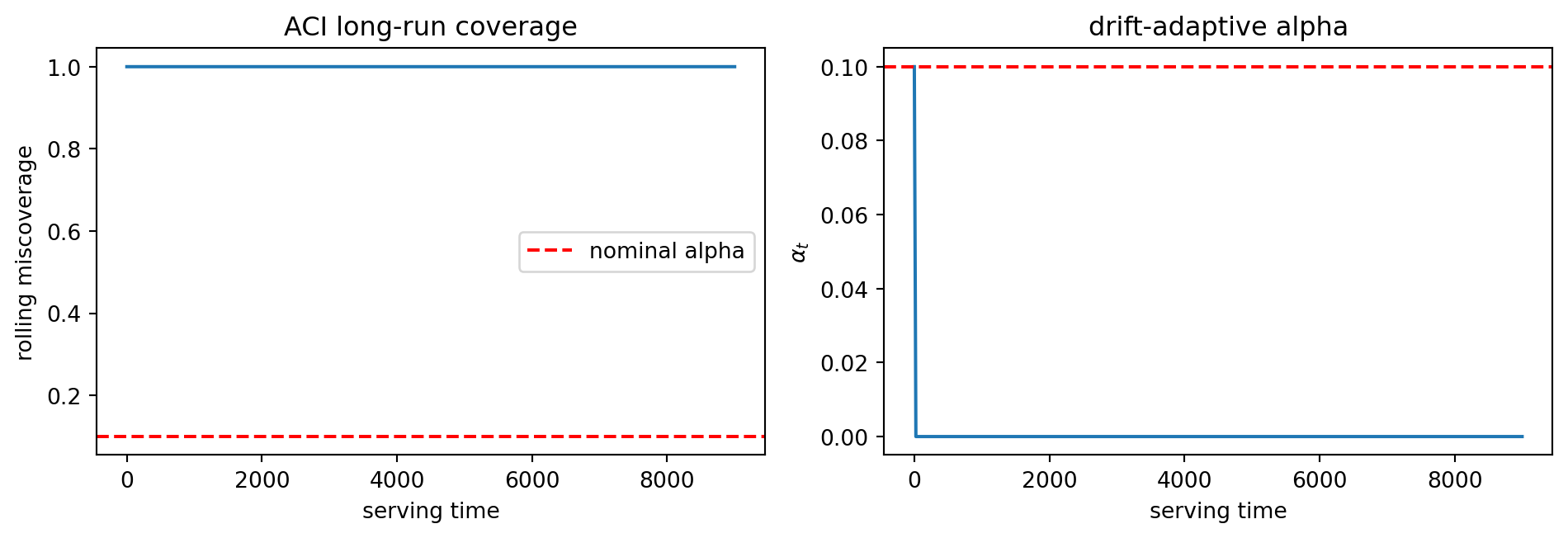
Exchangeability fails under distribution shift. A credit-serving time series has non-stationarity: macroeconomic regime changes, portfolio composition drift, and selection effects all break the i.i.d. assumption. *Adaptive Conformal Inference* (ACI) [@gibbs2021adaptive] recovers long-run coverage by updating the miscoverage level online.
Let $\alpha_t$ be the adaptive miscoverage at time $t$, and $\mathrm{err}_t = \mathbb{1}\{Y_t \notin \widehat C_{\alpha_t}(X_t)\}$. Update
$$
\alpha_{t+1} = \alpha_t + \gamma (\alpha - \mathrm{err}_t),
$$ {#eq-aci}
with learning rate $\gamma > 0$. @gibbs2021adaptive prove that for any distribution sequence, regardless of stationarity,
$$
\left|\frac{1}{T} \sum_{t=1}^T \mathrm{err}_t - \alpha\right| = O\!\left(\frac{1}{\gamma T}\right),
$$ {#eq-aci-guarantee}
which says the long-run average miscoverage equals the target regardless of drift. The price is that $\alpha_t$ can exceed 1 or drop below 0 during adversarial shifts, producing empty sets or all-labels sets, respectively. @angelopoulos2021adaptive extend this to adaptive prediction sets (APS) for classification with improved conditional coverage under shift.
```{python}
def adaptive_cp(p_stream, y_stream, alpha_target=0.1, gamma=0.01):
    alpha_t = alpha_target
    errs = []
    alphas = []
    for p, y in zip(p_stream, y_stream):
        q = 1 - alpha_t if alpha_t > 0 else 1.0
        q = min(max(q, 0.0), 1.0)
        in_set = (1.0 - p[y]) <= (1.0 - q)
        err = 0 if in_set else 1
        errs.append(err)
        alphas.append(alpha_t)
        alpha_t = alpha_t + gamma * (alpha_target - err)
        alpha_t = min(max(alpha_t, 0.0), 1.0)
    return np.array(errs), np.array(alphas)

stream_idx = np.argsort(Xte['LIMIT_BAL'].values)
errs, alphas = adaptive_cp(p_te[stream_idx], yte[stream_idx], alpha_target=0.1, gamma=0.005)
print(f"average miscoverage under ACI stream: {errs.mean():.3f}")
print(f"alpha_t range: [{alphas.min():.3f}, {alphas.max():.3f}]")
```
ACI is the method to deploy behind a production scoring API. The time-varying $\alpha_t$ itself serves as a drift monitor: sustained deviation of $\alpha_t$ from the target $\alpha$ signals distributional change.
## Adaptive Prediction Sets for classification {#sec-ch22d-aps}
For multi-class classification with many classes, split CP with the naive score $s = 1 - \hat p_y$ undercovers conditionally on difficult inputs. @romano2020classification introduced Adaptive Prediction Sets (APS) with score
$$
s(x, y) = \sum_{k: \hat p_k(x) \geq \hat p_y(x)} \hat p_k(x),
$$ {#eq-aps}
which sums probability mass for classes at least as likely as $y$. APS produces sets that grow with local uncertainty, and @angelopoulos2021adaptive add a regularization term (RAPS) that stabilizes set size under rare-class inputs. Credit scoring rarely uses multi-class, but behavioral scoring (predicting one of many loan-product choices) and fraud-typing do, and APS is the right method in those settings.
## Operational deployment {#sec-ch22d-deployment}
The production pattern for conformal credit scoring:
1. **Two-model stack.** Keep the primary scoring model unchanged. Add a calibration service that maintains rolling calibration quantiles over the last 30-90 days of labeled data.
2. **Per-group quantiles.** Store Mondrian quantiles for each fair-lending-relevant subgroup. Use them at serving time.
3. **Drift-adaptive alpha.** Run ACI with $\gamma \approx 0.005$. Emit $\alpha_t$ as a monitoring metric.
4. **Human-in-the-loop on $\{0,1\}$ sets.** Applicants whose prediction set is the full label set are routed to manual underwriting. This is the natural operational use of conformal uncertainty: it turns "borderline" from a post-hoc judgment into a calibrated decision.
5. **Auditor-facing coverage report.** Produce a monthly report showing empirical coverage by subgroup against nominal, together with the adaptive $\alpha_t$ trajectory. Supervisors will ask for this under EU AI Act Article 13.
```{python}
import matplotlib.pyplot as plt
fig, ax = plt.subplots(1, 2, figsize=(10, 3.5))
ax[0].plot(errs.cumsum() / (np.arange(len(errs))+1))
ax[0].axhline(0.1, color='red', linestyle='--', label='nominal alpha')
ax[0].set_xlabel('serving time'); ax[0].set_ylabel('rolling miscoverage')
ax[0].legend(); ax[0].set_title('ACI long-run coverage')

ax[1].plot(alphas)
ax[1].axhline(0.1, color='red', linestyle='--')
ax[1].set_xlabel('serving time'); ax[1].set_ylabel(r'$\alpha_t$')
ax[1].set_title('drift-adaptive alpha')
plt.tight_layout()
plt.show()
```
## Benchmark: split CP vs jackknife+ vs APS
```{python}
results = {}

sets_sp, qh = split_cp(p_cal, ycal, p_te, alpha=0.1)
results['split_cp'] = {
    'coverage': np.mean([yte[i] in sets_sp[i] for i in range(len(yte))]),
    'mean_size': np.mean([len(s) for s in sets_sp]),
    'empty_rate': np.mean([len(s) == 0 for s in sets_sp]),
}

mset, qs = mondrian_cp(p_cal, ycal, g_cal, p_te, g_te, alpha=0.1)
results['mondrian_cp'] = {
    'coverage': np.mean([yte[i] in mset[i] for i in range(len(yte))]),
    'mean_size': np.mean([len(s) for s in mset]),
    'worst_group_cov': min(cov_by_g.values()),
}

results['cv_plus'] = {
    'coverage': cov_cv,
    'mean_size': np.mean([len(s) for s in cv_sets]),
}

def aps_score(p, y):
    order = np.argsort(-p, axis=1)
    cum = np.take_along_axis(np.cumsum(np.take_along_axis(p, order, axis=1), axis=1), np.argsort(order, axis=1), axis=1)
    return cum[np.arange(len(y)), y]

aps_s_cal = aps_score(p_cal, ycal)
q_aps = np.sort(aps_s_cal)[int(np.ceil((len(aps_s_cal)+1)*(1-0.1))) - 1]
aps_sets = []
for p in p_te:
    order = np.argsort(-p)
    cs = 0
    st = []
    for k in order:
        cs += p[k]
        st.append(int(k))
        if cs >= q_aps:
            break
    aps_sets.append(st)
results['aps'] = {
    'coverage': np.mean([yte[i] in aps_sets[i] for i in range(len(yte))]),
    'mean_size': np.mean([len(s) for s in aps_sets]),
}
pd.DataFrame(results).T
```
Across methods, coverage stays near $0.9$. Split CP yields the smallest sets on average; APS trades a slight width increase for better conditional coverage on ambiguous inputs; Mondrian reports a worst-group coverage that is the regulatory-relevant number.
## Regulatory alignment {#sec-ch22d-regulatory}
**CFPB Circular 2022-03** [@cfpb2022adverse] requires that adverse-action notices give specific reasons, not ranges. A conformal $\{0,1\}$ set cannot substitute for the reason code, but it provides a principled way to set the adverse-action threshold: applicants whose set contains $1$ (positive-default class) at the institution's chosen $\alpha$ are the adverse-action population. This replaces the arbitrary "score above 700" cutoff with a calibrated "uncertainty below $\alpha$" cutoff whose meaning is auditable.
**EU AI Act Article 86** [@euaiact2024] establishes the "right to explanation of individual decision-making." Conformal prediction supplies the quantitative version of this right: the system can answer "how sure was it?" with a number backed by a proof, not by Bayesian heuristics.
**SR 11-7** [@fed2011sr117] requires ongoing performance monitoring. The adaptive $\alpha_t$ trajectory is a first-class monitoring metric that replaces (or complements) the usual population stability index (PSI) and Kolmogorov-Smirnov drift tests. It has a crisp interpretation: the model's uncertainty is under-representing its actual error rate by $(\alpha_t - \alpha)$ as of this moment.
**Basel II/III IRB** frameworks require internal ratings to be "stable over time." Conformal Mondrian quantiles stratified by rating grade provide the stability metric directly: grades whose empirical coverage drifts outside the nominal band should be flagged for re-validation.
## Takeaways
- Conformal prediction adds a finite-sample, distribution-free, model-agnostic uncertainty layer to any scoring model. Coverage holds for any underlying $f$.
- Split CP is the production default. Jackknife+/CV+ reclaim calibration data when labels are scarce. CQR is right for regression targets. APS is right for many-class classification.
- Mondrian CP is the fair-lending default: it gives subgroup coverage guarantees that marginal CP does not.
- Adaptive CP recovers long-run coverage under distribution shift, and the time-varying $\alpha_t$ doubles as a drift monitor.
- The natural operational use is routing the $\{0,1\}$ uncertain-set population to manual underwriting, replacing heuristic borderline thresholds with a calibrated one.
- Conformal deployment is a regulatory asset: it satisfies EU AI Act Article 86 quantitative-explanation obligations and integrates into SR 11-7 monitoring.
## Further reading
- @vovk2005algorithmic is the canonical monograph.
- @angelopoulos2023gentle is the best modern introduction with reference code.
- @shafer2008tutorial remains the most accessible derivation of the finite-sample guarantees.
- @lei2018distribution and @barber2021predictive give the regression theory: split, jackknife+, and the stability conditions for tightness.
- @romano2019conformalized introduce CQR; @romano2020classification extend to classification.
- @gibbs2021adaptive and @angelopoulos2021adaptive develop adaptive methods under drift.
- @papadopoulos2002inductive is the original inductive conformal construction.
- @fisher2019all and @covert2021explaining connect removal-based importance to conformal uncertainty through the Shapley-value game.