---
execute:
echo: true
eval: true
---
# Reject Inference and Sample Selection {#sec-ch10}
::: {.callout-note appearance="simple" icon="false"}
**Scope: retail.** Reject inference for application scoring on consumer portfolios, where rejected-applicant volumes are large enough to fit the parametric MNAR machinery developed here. Corporate originations are too heterogeneous and too small a sample for the same approach.
:::
## Overview {.unnumbered}
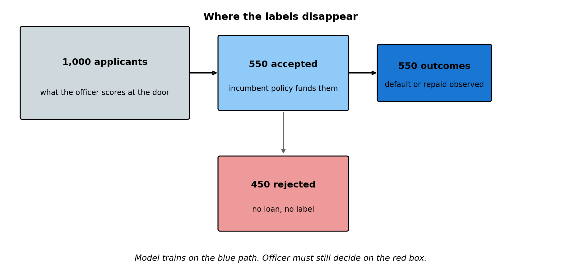
A lender's data generation process is not i.i.d. from the applicant population. Only the accepted see a loan, and only the accepted produce an outcome we can label. Every estimator that trains on accepted-only data, and every validation curve drawn from accepted-only data, therefore answers a different question than the one a credit officer is asking. The officer asks: what is the probability of default for this applicant in the unrestricted pool? The accepted-only model answers: what is the probability of default for applicants who resemble those the incumbent policy chose to fund?
Two pictures fix the geometry before any algebra. @fig-ch10-visibility-funnel shows where labels disappear in the data pipeline. @fig-ch10-conditional-shift shows what that disappearance does to the curves a modeler actually plots.
```{python}
#| label: fig-ch10-visibility-funnel
#| fig-cap: "From applicants to labels. Of every 1,000 through-the-door applicants, the incumbent policy funds roughly 550 and the bureau later returns a default-or-repaid outcome on those 550. The other 450 produce no label. Any model trained on the blue path is fit on the funded slice only; the credit officer must still answer for the red box at decision time."
import matplotlib.pyplot as plt
import matplotlib.patches as mpatches

fig, ax = plt.subplots(figsize=(9.5, 4.8))
ax.set_xlim(0, 10)
ax.set_ylim(0, 6)
ax.axis("off")

def box(x, y, w, h, color, label, sublabel):
    rect = mpatches.FancyBboxPatch(
        (x, y), w, h, boxstyle="round,pad=0.04",
        facecolor=color, edgecolor="black", linewidth=1.2,
    )
    ax.add_patch(rect)
    ax.text(x + w / 2, y + h * 0.62, label,
            ha="center", va="center", fontsize=11, fontweight="bold")
    ax.text(x + w / 2, y + h * 0.28, sublabel,
            ha="center", va="center", fontsize=9)

box(0.3, 3.5, 3.0, 2.0, "#cfd8dc",
    "1,000 applicants", "what the officer scores at the door")
box(3.9, 3.7, 2.3, 1.6, "#90caf9",
    "550 accepted", "incumbent policy funds them")
box(6.8, 3.9, 2.0, 1.2, "#1976d2",
    "550 outcomes", "default or repaid observed")
box(3.9, 1.0, 2.3, 1.6, "#ef9a9a",
    "450 rejected", "no loan, no label")

ax.annotate("", xy=(3.88, 4.5), xytext=(3.32, 4.5),
            arrowprops=dict(arrowstyle="-|>", lw=1.4))
ax.annotate("", xy=(6.78, 4.5), xytext=(6.22, 4.5),
            arrowprops=dict(arrowstyle="-|>", lw=1.4))
ax.annotate("", xy=(5.05, 2.65), xytext=(5.05, 3.65),
            arrowprops=dict(arrowstyle="-|>", lw=1.4, color="0.4"))

ax.text(5.0, 0.35,
        "Model trains on the blue path. Officer must still decide on the red box.",
        ha="center", va="center", fontsize=10, style="italic")
ax.text(5.0, 5.75,
        "Where the labels disappear",
        ha="center", va="center", fontsize=12, fontweight="bold")

plt.tight_layout()
plt.show()
```
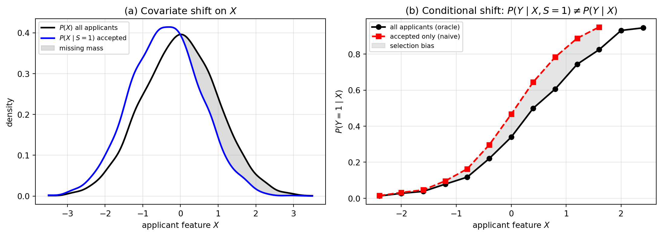
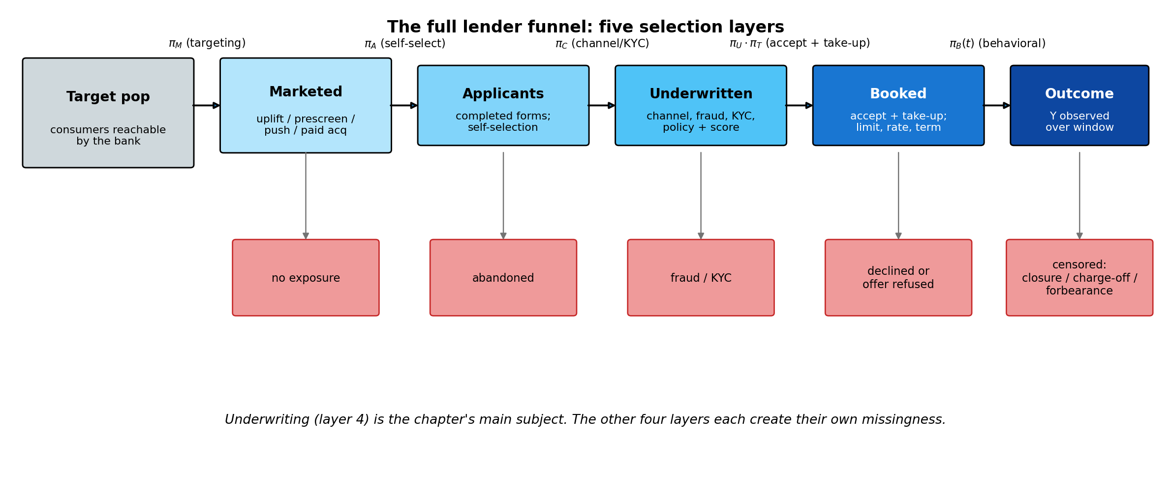
The funnel is descriptive. The substantive damage is visible on a default-rate curve. @fig-ch10-conditional-shift shows what happens when we draw the same plot using the full applicant population (which we know only because this is a simulation) and using the accepted slice (which is all a real lender ever sees). The three-box version of the funnel collapses several real selection layers (pre-application targeting, application self-selection, channel and KYC gates, take-up, and post-booking management) into a single accept/decline arrow; @sec-ch10-full-funnel returns to the full five-layer view and gives a separate correction for each layer.
```{python}
#| label: fig-ch10-conditional-shift
#| fig-cap: "Two faces of the selection problem on a synthetic through-the-door population (n = 8,000) with bivariate-normal correlation $\\rho = 0.6$ between the latent default error and the latent acceptance error. (a) Covariate shift: the accepted-population density of the feature $X$ is pulled toward the safer (lower-$X$) side because the policy declines high-$X$ applicants. (b) Conditional shift: the empirical default rate plotted against $X$ is uniformly higher on the accepted slice than on the through-the-door population, even after conditioning on $X$, because the policy accepts on a latent signal positively correlated with the default error. The shaded gap in (b) is the bias that reject inference must close; it cannot be removed by reweighting on $X$ alone because it comes from selection on the unobserved error, not from feature imbalance."
import numpy as np
import matplotlib.pyplot as plt
from scipy import stats
from scipy.stats import gaussian_kde

rng_fig = np.random.default_rng(20260428)
n_fig = 8_000
X_fig = rng_fig.standard_normal(n_fig)
Z_fig = rng_fig.standard_normal(n_fig)

rho_fig = 0.6
u_fig = rng_fig.standard_normal(n_fig)
v_fig = rho_fig * u_fig + np.sqrt(1 - rho_fig**2) * rng_fig.standard_normal(n_fig)

y_star_fig = -0.4 + 0.9 * X_fig + u_fig
y_fig = (y_star_fig > 0).astype(int)

s_star_fig = -0.7 * X_fig + 0.9 * Z_fig + v_fig
s_fig = (s_star_fig > 0).astype(int)

fig, axes = plt.subplots(1, 2, figsize=(11.5, 4.2))

ax = axes[0]
xs = np.linspace(-3.5, 3.5, 400)
kde_all = gaussian_kde(X_fig)(xs)
kde_acc = gaussian_kde(X_fig[s_fig == 1])(xs)
ax.plot(xs, kde_all, "k-",  lw=2.0, label=r"$P(X)$ all applicants")
ax.plot(xs, kde_acc, "b-",  lw=2.0, label=r"$P(X \mid S=1)$ accepted")
ax.fill_between(xs, kde_all, kde_acc, where=(kde_all > kde_acc),
                color="0.7", alpha=0.45, label="missing mass")
ax.set_xlabel(r"applicant feature $X$")
ax.set_ylabel("density")
ax.set_title("(a) Covariate shift on $X$")
ax.legend(fontsize=8, loc="upper left")
ax.grid(alpha=0.3)

ax = axes[1]
bins = np.linspace(-3, 3, 16)
mid = 0.5 * (bins[:-1] + bins[1:])

def binmean(mask):
    out = np.full_like(mid, np.nan, dtype=float)
    for i in range(len(mid)):
        m = mask & (X_fig >= bins[i]) & (X_fig < bins[i + 1])
        if m.sum() > 30:
            out[i] = y_fig[m].mean()
    return out

emp_all = binmean(np.ones(n_fig, dtype=bool))
emp_acc = binmean(s_fig == 1)
ax.plot(mid, emp_all, "ko-",  lw=2.0, label="all applicants (oracle)")
ax.plot(mid, emp_acc, "rs--", lw=2.0, label="accepted only (naive)")
valid = np.isfinite(emp_all) & np.isfinite(emp_acc)
ax.fill_between(mid[valid], emp_all[valid], emp_acc[valid],
                color="0.75", alpha=0.4, label="selection bias")
ax.set_xlabel(r"applicant feature $X$")
ax.set_ylabel(r"$P(Y=1 \mid X)$")
ax.set_title(r"(b) Conditional shift: $P(Y \mid X, S=1) \neq P(Y \mid X)$")
ax.legend(fontsize=8, loc="upper left")
ax.grid(alpha=0.3)

plt.tight_layout()
plt.show()
```
Panel (a) is what reweighting fixes: the feature distribution differs between funded and through-the-door, and inverse probability weights on $X$ recover $P(X)$ from $P(X \mid S=1)$. Panel (b) is what reweighting cannot fix: even at the same $X$, the accepted applicants default *more*, because the underwriter accepted on signals that we never recorded and that also predict default. (The opposite sign of the gap, accepted defaulting *less*, would arise if the underwriting signals were negatively correlated with the default error, i.e. effective screening on unobservables; we treat both regimes symmetrically when we discuss the sign of $\hat\rho$ in @sec-ch10-heckman-selection-correction.) That is the part of the gap that motivates Heckman, the impossibility result, and everything that follows in this chapter.
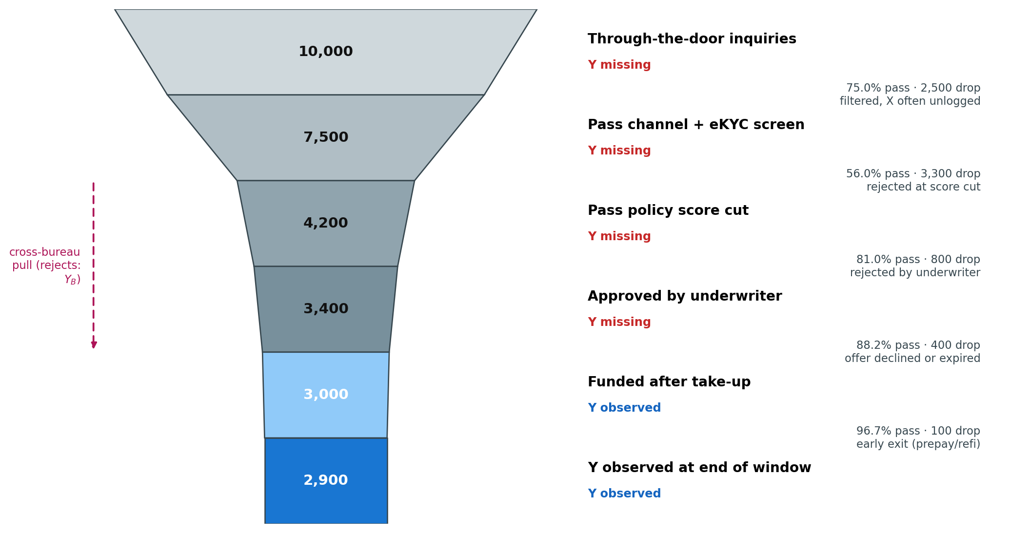
Before tackling the methods in turn, it helps to map every stage where selection bias enters and every identification condition a corrective method might lean on. We use three views in turn. @fig-ch10-funnel-volumes plots the typical drop-off in counts at each gate, so the order-of-magnitude problem is visible at a glance. @fig-ch10-selection-roadmap is a stage-level DAG of the same pipeline, with the labelled exits where $Y$ is missing or imported from a bureau. @tbl-ch10-bias-dimensions then catalogues the seven *selection-bias dimensions* (D1 through D7) that any reject inference exercise has to take an explicit position on, the stage at which each one binds, and the section of the chapter that addresses it. A note on terminology. We call D1 through D7 *selection-bias dimensions* (or *identification checkpoints*) rather than *moderators*: in the standard statistical usage a moderator is a variable that interacts with $X$ to shift the $X \to Y$ relationship, whereas D1 through D7 are a mix of bias *sources* (D2, D3), positivity and identification *assumptions* (D1, D4), and external-validity *threats* (D5, D6, D7). Each subsequent section of the chapter targets one or more of these dimensions, and the impossibility result of @sec-ch10-impossibility says exactly which combinations the accepted-only sample can never settle on its own.
```{python}
#| label: fig-ch10-funnel-volumes
#| fig-cap: "Typical drop-off through a Vietnamese consumer-finance acquisition funnel for 10,000 through-the-door inquiries. Band widths are proportional to surviving counts; the right column reads off the absolute count, the labelled-Y indicator, and the stage-to-stage pass rate. Only the bottom two bands carry an observed default outcome $Y$ for the lender; the rejected (red) band is the population that bureau extrapolation tries to recover, and the filtered (grey) band is the population whose features were never even logged. The funded slice is roughly 30 percent of the through-the-door pool, yet a naive PD model can only be trained on it."
import matplotlib.pyplot as plt
import matplotlib.patches as mpatches
import numpy as np

stages = [
    ("Through-the-door inquiries",      10_000, "#cfd8dc", False, None),
    ("Pass channel + eKYC screen",       7_500, "#b0bec5", False, "filtered, X often unlogged"),
    ("Pass policy score cut",            4_200, "#90a4ae", False, "rejected at score cut"),
    ("Approved by underwriter",          3_400, "#78909c", False, "rejected by underwriter"),
    ("Funded after take-up",             3_000, "#90caf9", True,  "offer declined or expired"),
    ("Y observed at end of window",      2_900, "#1976d2", True,  "early exit (prepay/refi)"),
]
counts = np.array([c for _, c, _, _, _ in stages], dtype=float)
labels = [s for s, _, _, _, _ in stages]
colors = [c for _, _, c, _, _ in stages]
y_obs  = [yo for _, _, _, yo, _ in stages]
drop_reasons = [r for _, _, _, _, r in stages]
top = counts.max()
widths = counts / top

fig, ax = plt.subplots(figsize=(11, 5.8))
ax.set_xlim(-0.7, 1.6)
ax.set_ylim(0, len(stages))
ax.invert_yaxis()
ax.axis("off")

def trapezoid(y, w_top, w_bot, color):
    cx = 0.0
    pts = [
        (cx - w_top / 2, y),
        (cx + w_top / 2, y),
        (cx + w_bot / 2, y + 1),
        (cx - w_bot / 2, y + 1),
    ]
    poly = mpatches.Polygon(pts, closed=True, facecolor=color,
                            edgecolor="#37474f", linewidth=1.0)
    ax.add_patch(poly)

for i in range(len(stages)):
    w_top = widths[i]
    w_bot = widths[i + 1] if i + 1 < len(stages) else widths[i]
    trapezoid(i, w_top, w_bot, colors[i])
    ax.text(0.0, i + 0.5, f"{int(counts[i]):,}",
            ha="center", va="center", fontsize=11,
            color="white" if i >= len(stages) - 2 else "#111",
            fontweight="bold")

    badge = "Y observed" if y_obs[i] else "Y missing"
    badge_color = "#1565c0" if y_obs[i] else "#c62828"
    ax.text(0.62, i + 0.35, labels[i],
            ha="left", va="center", fontsize=10.5, fontweight="bold")
    ax.text(0.62, i + 0.65, badge,
            ha="left", va="center", fontsize=9, color=badge_color,
            fontweight="bold")
    if i + 1 < len(stages):
        conv = counts[i + 1] / counts[i] * 100
        drop = int(counts[i] - counts[i + 1])
        reason = drop_reasons[i + 1] or ""
        ax.text(1.55, i + 1, f"{conv:4.1f}% pass · {drop:,} drop\n{reason}",
                ha="right", va="center", fontsize=8.5, color="#37474f")

ax.annotate("", xy=(-0.55, 4.0), xytext=(-0.55, 2.0),
            arrowprops=dict(arrowstyle="-|>", lw=1.4,
                            linestyle=(0, (4, 3)), color="#ad1457"))
ax.text(-0.58, 3.0, "cross-bureau\npull (rejects:\n$Y_B$)",
        ha="right", va="center", fontsize=8.5, color="#ad1457")

plt.tight_layout()
plt.show()
```
::: no-panzoom
```{mermaid}
%%| label: fig-ch10-selection-roadmap
%%| fig-cap: "Stage-level DAG of the selection pipeline. Solid arrows are the funded path on which $Y$ is observed; red boxes mark exits where $Y$ is missing for the lender; dotted arrows are optional ports where the lender can pull a bureau outcome $Y_B$ on rejected applicants. The seven selection-bias dimensions D1 through D7 are catalogued in @tbl-ch10-bias-dimensions; this diagram intentionally omits the dimension labels from the nodes so the pipeline structure stays legible."
flowchart TD
    classDef stage fill:#eceff1,stroke:#455a64,color:#111;
    classDef gate  fill:#fff8e1,stroke:#b58900,color:#111;
    classDef obs   fill:#1976d2,stroke:#0d47a1,color:#fff;
    classDef miss  fill:#ef9a9a,stroke:#c62828,color:#111;
    classDef bureau fill:#f8bbd0,stroke:#ad1457,color:#111;

    A["Through-the-door applicant<br/>X observed, Z partial, U and V latent"]:::stage
    S1{{"Stage 1: channel and eKYC screen"}}:::gate
    L1["Filtered pre-score<br/>X often not stored"]:::miss
    S2{{"Stage 2: policy and underwriter decision"}}:::gate
    REJ["Rejected (S=0)<br/>Y missing for the lender"]:::miss
    YB["Bureau outcome Y_B<br/>different lender, different product"]:::bureau
    ACC["Funded (S=1)<br/>limit, rate, term"]:::stage
    PW{{"Stage 3: performance window<br/>vintage v, macro state m"}}:::gate
    PRP["Prepay or refinance<br/>competing event (ch 9)"]:::miss
    Y["Outcome Y observed"]:::obs

    A --> S1
    S1 -->|fail| L1
    S1 -->|pass| S2
    S2 -->|S=0| REJ
    S2 -->|S=1| ACC
    REJ -.->|cross-bureau pull| YB
    ACC --> PW
    PW --> Y
    PW -.->|early exit| PRP
```
:::
| ID | Selection-bias dimension | Stage where it binds | Section that addresses it |
|------------------|------------------|------------------|-------------------|
| D1 | Policy overlap: is $P(S{=}1 \mid x) > 0$ everywhere on the support of $X$? | Stage 1 hard pre-screens; Stage 2 score cut | @sec-ch10-observable, @sec-ch10-rdd |
| D2 | Covariate shift on $X$: $P(X \mid S{=}1) \neq P(X)$ | Stage 2 (and Stage 1 if it depends on $X$) | @sec-ch10-augmentation-hsias-parceling-and-its-fuz, @sec-ch10-modern |
| D3 | Selection on unobservables: $\mathrm{Corr}(U,V) \neq 0$ | Stage 2 (underwriter signals not in $X$) | @sec-ch10-heckman-selection-correction, @sec-ch10-modern |
| D4 | Exclusion restriction: a $Z$ that shifts $S$ but not $Y$ | Stage 2 (assumption about the design) | @sec-ch10-heckman-selection-correction |
| D5 | Vintage and macro state: through-the-cycle vs point-in-time | Stage 3 performance window | @sec-ch10-targeting, @sec-ch10-behavioral |
| D6 | Bureau product gap: limit, rate, servicer differ from the lender's product | Bureau path on rejects | @sec-ch10-bureau-extrapolation |
| D7 | Within-reject bureau coverage: 10 to 30 percent of rejects have no trade-line | Bureau path on rejects | @sec-ch10-bureau-extrapolation |
: Seven selection-bias dimensions that every reject-inference method must take a position on. Each row names the stage of @fig-ch10-selection-roadmap at which the dimension first binds, and the section of the chapter where it is treated. {#tbl-ch10-bias-dimensions}
A short reading guide. Augmentation and parceling (@sec-ch10-augmentation-hsias-parceling-and-its-fuz) leans on D2 alone and assumes D3 away. Bureau extrapolation (@sec-ch10-bureau-extrapolation) buys D3 by importing $Y_B$ but inherits D5, D6, and D7. Heckman (@sec-ch10-heckman-selection-correction) trades D3 for parametric structure plus D4. AIPW, copulas, deep generative imputation, importance weighting, and PU learning (@sec-ch10-modern) each relax one Heckman primitive. Observable-engine methods (@sec-ch10-observable) attack D1 directly when the lender owns the decision engine. EM and pseudo-labeling (@sec-ch10-em) exploit cluster structure when none of the above is available.
This chapter treats the gap between those two questions as the subject in its own right. We formalize the missing-data taxonomy (@sec-ch10), derive the Heckman (1979) two-step selection correction in full (@sec-ch10-heckman-selection-correction), state and prove the Hand and Henley (1997) impossibility result (@sec-ch10-impossibility), and write the EM algorithm that underpins a self-training reject inference loop (@sec-ch10-em). We then go beyond Heckman with five modern estimators: doubly robust AIPW (@robins1994estimation, @chernozhukov2018double), copula-based selection (@marra2017bivariate), deep generative imputation (@mancisidor2020deep), covariate-shift importance weighting (@sugiyama2007covariate, @bickel2009discriminative), and positive-unlabeled learning (@kiryo2017positive). A separate strand handles the case where the lender observes its own decision engine, where regression-discontinuity (@hahn2001identification, @imbens2008recent) and exact-propensity weighting recover identification without parametric assumptions. A method-agnostic AIPW score unifies these threads and translates one-for-one to the survival-censoring problem of @sec-ch09 and to LDA, gradient boosting, and lifetime PD elsewhere in the book. We close with two modern practitioner views: the marketplace-lending perspective of @vallee2019marketplace and the automation/disparity evidence of @howell2024lender.
The chapter is deliberately not a tour of reject inference recipes. The recipes without the identifiability argument behind them are dangerous in production, because a plausible looking PD curve on rejected applicants can coexist with arbitrarily wrong truth. That is the Hand and Henley point, and the rest of the chapter is an attempt to meet it with either extra structure (exclusion restrictions, parametric families) or extra data (bureau outcomes, through-the-door bureau vintages).
The problem is most severe in emerging markets. A Vietnamese consumer lender rolling out eKYC under Circular 16/2020/TT-NHNN sees through-the-door volumes ten times its booked volume, decline rates above 70 percent are routine at the consumer-finance subsidiaries of joint-stock banks, and CIC lookups skew toward the thinnest of thin files [@sbv2020ekyc; @cicvn2023report]. Informal income, Tet-induced cash-flow compression, and macro volatility mean the selection rule correlates with unobservables that also drive default. The closing emerging-market section returns to this with CIC-based bureau extrapolation, Heckman exclusion candidates specific to Vietnam, and Decree 13/2023 constraints on how rejected-applicant data can be retained and reused.
## Notation {#sec-ch10-notation .unnumbered}
Let $X \in \mathbb{R}^p$ be the application features observed at decision time, $Z \in \mathbb{R}^q$ be a vector used in the selection decision but excluded from the outcome equation, and $Y \in \{0,1\}$ the default indicator over a fixed performance window. Let $S \in \{0,1\}$ be the accept indicator ($S=1$ if the incumbent policy funded the loan). Only $(X, Z, S)$ are observed for the full through-the-door population. $Y$ is observed only when $S = 1$.
Throughout the chapter, $\phi$ and $\Phi$ denote the standard normal density and CDF. The inverse Mills ratio is $\lambda(a) = \phi(a)/\Phi(a)$. Expectations over the unobserved error vector $(u, v)$ respect the bivariate normal joint structure assumed in @heckman1979sample, with correlation $\rho$ and outcome-side standard deviation $\sigma$ (normalized to 1 in the probit case).
**Nuisance functions.** []{#sec-ch10-nuisance-def} The chapter uses the word *nuisance* in its semiparametric-statistics sense, not its everyday sense. The *parameter of interest* (also called the target functional) is the object the lender actually wants to estimate: the through-the-door PD $\mu_0(x) = P(Y = 1 \mid X = x)$, the scorecard coefficients $\beta$, the dollar expected loss on a policy region, or any other functional of the full-population law. A *nuisance function* (or *nuisance parameter* when finite-dimensional) is any other quantity that the estimator needs as an input but that the lender does not care about reporting. In this chapter the two recurring nuisances are the propensity $\pi(x, z) = P(S = 1 \mid X = x, Z = z)$ (the probability the incumbent policy accepts an applicant with features $(x, z)$) and the accept-conditional outcome regression $g(x) = \mathbb{E}[Y \mid X = x, S = 1]$ (the booked-sample default rate at $X = x$). In plain English, $\pi$ models *who gets in* and $g$ models *how the people who got in performed*; neither is the answer the credit officer wants, but the AIPW score $\hat\mu(x) = g(x) + (S / \pi(x, z))(Y - g(x))$ needs both to recover the through-the-door PD. The name *nuisance* is historical (the term goes back to @neyman1948consistent and the semiparametric efficiency literature collected in @vandervaart1998asymptotic): these functions are a *nuisance* because their estimation error has to be controlled to get a clean inference statement on the parameter of interest, even though their values are not themselves the answer. Two practical consequences of this framing recur in the chapter. (i) *A nuisance can be misspecified and the estimator still consistent.* AIPW is *doubly robust* precisely in the sense that if either $\pi$ or $g$ equals the truth, the estimator recovers $\mu_0$ even when the other nuisance is wrong (@sec-ch10-heckman-vs-dml). (ii) *Nuisances can be fit by arbitrary machine learning.* Under Neyman orthogonality and cross-fitting, both $\hat\pi$ and $\hat g$ are allowed to converge at the slow $o(n^{-1/4})$ rate that flexible learners like gradient boosting deliver, and the second-stage estimator of the parameter of interest still inherits the textbook $\sqrt n$ rate and a usable confidence interval (@chernozhukov2018double, formalized at @eq-dml-rate). In a survival or expected-loss extension the nuisance pair generalizes naturally: $\pi$ becomes a censoring or selection hazard, $g$ becomes a conditional survival or loss surface, but the role in the estimator stays the same.
## The selection bias problem {#sec-ch10-reject}
### The naive fit and what it estimates
Fix the incumbent policy as a deterministic rule $s(x, z)$ with $S = s(X, Z)$ almost surely (we relax this later). The lender observes $\{(X_i, Z_i, Y_i) : S_i = 1\}$. A naive maximum-likelihood fit of a PD model $P(Y=1 \mid X; \beta)$ on this sample estimates
$$
\beta_{\text{naive}} = \arg\max_\beta \mathbb{E}\big[ \log P(Y \mid X; \beta) \big\vert S = 1 \big].
$$ {#eq-naive-target}
The target is the conditional on $S=1$. When the decision rule depends on $X$, the feature marginal $P(X \mid S=1)$ is shifted relative to $P(X)$. When the decision rule also correlates with unobservables that drive $Y$, the conditional $P(Y \mid X, S=1)$ is shifted relative to $P(Y \mid X)$. The first shift is covariate shift, fixable with reweighting when the target distribution is known. The second shift is selection bias proper, and it is what reject inference tries to repair.
The distinction matters because there exist rules that induce covariate shift without selection bias. If $s(X, Z) = \mathbf{1}\{Z > 0\}$ and $Z$ is independent of $(Y, X)$, then $P(Y \mid X, S=1) = P(Y \mid X)$ and there is nothing to correct. The pathology is when $s$ depends on $X$ in a way that covaries with the residual in the outcome model, or when $s$ depends on latent information unobserved to the modeler that is also predictive of $Y$. In consumer credit both are the norm. Loan officers read free-text notes, underwriters flag informal income, overlays include desk-level intuition, and all of that ends up baked into the accept decision but absent from the feature store.
### Two mechanisms {#sec-ch10-two-mechanisms}
To make the distinction concrete, fix one outcome model and run two selection rules through it. The outcome model has one observable feature $X$ and one latent residual $U$ that stands in for everything not in the feature store: informal-income flags, free-text underwriter notes, desk overlays. Two selection rules differ only in what drives the accept decision. @fig-ch10-two-mechanisms-a and @fig-ch10-two-mechanisms-b show the mechanism graphs in turn; the only structural difference is the arrow into $S$ in the second graph. In both graphs $Y$ is the latent default that *would* be realized if the applicant were funded; $S$ governs whether we observe $Y$, not whether it occurs, which is why no arrow runs from $S$ into $Y$.
::: no-panzoom
```{mermaid}
%%| label: fig-ch10-two-mechanisms-a
%%| fig-cap: "Scenario A: covariate shift only. Squares are observed at decision time; dashed circles are latent residuals the modeler does not see. The accept rule depends on observable $X$ and an independent noise $W$, so $P(X \\mid S=1)$ shifts relative to $P(X)$ but the conditional $P(Y \\mid X)$ is preserved. Reweighting on $X$ alone closes the gap."
flowchart TB
classDef obs fill:#cfd8dc,stroke:#37474f,color:#111;
classDef lat fill:#fff,stroke:#c62828,color:#c62828;
classDef noise fill:#fff,stroke:#90a4ae,color:#455a64;
classDef sel fill:#90caf9,stroke:#0d47a1,color:#111;
classDef out fill:#1976d2,stroke:#0d47a1,color:#fff;
XA["X<br/>features"]:::obs
UA(("U<br/>latent residual")):::lat
WA(("W<br/>noise, indep of U")):::noise
SA{{"S<br/>accept if W > X"}}:::sel
YA["Y<br/>default"]:::out
XA --> YA
UA --> YA
XA --> SA
WA --> SA
```
:::
::: no-panzoom
```{mermaid}
%%| label: fig-ch10-two-mechanisms-b
%%| fig-cap: "Scenario B: selection bias proper. The accept rule depends on a latent $V$ correlated with the outcome residual $U$ (correlation $\\rho$). The marginal $P(X \\mid S=1)$ is identical to Scenario A by construction, so both induce the same covariate shift, but here the conditional $P(Y \\mid X, S=1) \\ne P(Y \\mid X)$. That single arrow from $U$ into $V$ is what reject inference exists to address."
flowchart TB
classDef obs fill:#cfd8dc,stroke:#37474f,color:#111;
classDef lat fill:#fff,stroke:#c62828,color:#c62828;
classDef sel fill:#90caf9,stroke:#0d47a1,color:#111;
classDef out fill:#1976d2,stroke:#0d47a1,color:#fff;
XB["X<br/>features"]:::obs
UB(("U<br/>latent residual")):::lat
VB(("V<br/>Corr with U = 0.6")):::lat
SB{{"S<br/>accept if V > X"}}:::sel
YB["Y<br/>default"]:::out
XB --> YB
UB --> YB
XB --> SB
VB --> SB
UB -.->|rho| VB
```
:::
Now drive the two graphs through a simulation. Both scenarios share the through-the-door feature $X$, the outcome residual $U$, and the outcome rule $Y = \mathbf{1}\{0.7X + U > 0.5\}$. Scenario A's accept rule depends on an independent noise $W$, so within any $X$-bin the accept slice is a uniform random subsample of the bin and inherits the bin's $U$ distribution. Scenario B's accept rule depends on $V$ with $\mathrm{Corr}(U, V) = 0.6$, so within any $X$-bin the accepted ones are exactly the applicants with the highest $V$, which by correlation are the applicants with the highest $U$, which by the outcome rule are the applicants most likely to default. The marginal accept rate and the marginal $P(X \mid S=1)$ are identical across the two scenarios by construction.
```{python}
#| label: tbl-ch10-two-mechanisms
#| tbl-cap: "Default rate within $X$-bins on a synthetic through-the-door population (n = 200,000). The full-population column is the truth a credit officer wants. Scenario A's accept-only column matches the truth bin-by-bin within Monte-Carlo noise: the accept rule is independent of the outcome residual, so covariate shift skews the support of $X$ but not the conditional. Scenario B's accept-only column is uniformly higher than the truth: even within a fixed $X$-bin, accepts are the applicants with the highest $V$, and $V$ is correlated with $U$ which drives $Y$. The B-minus-truth column is the bias that reweighting on $X$ alone cannot close."
import numpy as np
import pandas as pd

rng = np.random.default_rng(20260503)
n = 200_000
rho = 0.6

U = rng.standard_normal(n)
V = rho * U + np.sqrt(1.0 - rho**2) * rng.standard_normal(n)
W = rng.standard_normal(n)
X = rng.standard_normal(n)

Y = ((0.7 * X + U) > 0.5).astype(int)
S_A = ((W - X) > 0.0).astype(int)
S_B = ((V - X) > 0.0).astype(int)

bin_edges = np.array([-2.0, -1.0, -0.5, 0.0, 0.5, 1.0, 2.0])
rows = []
for lo, hi in zip(bin_edges[:-1], bin_edges[1:]):
    in_bin = (X >= lo) & (X < hi)
    p_truth = Y[in_bin].mean()
    p_A = Y[in_bin & (S_A == 1)].mean()
    p_B = Y[in_bin & (S_B == 1)].mean()
    rows.append({
        "X bin": f"[{lo:+.1f}, {hi:+.1f})",
        "n in bin": int(in_bin.sum()),
        "P(Y=1|X) truth": f"{p_truth:.3f}",
        "Scenario A P(Y=1|X,S=1)": f"{p_A:.3f}",
        "Scenario B P(Y=1|X,S=1)": f"{p_B:.3f}",
        "B - truth": f"{p_B - p_truth:+.3f}",
    })

print(pd.DataFrame(rows).to_string(index=False))

print(
    f"\nMarginal accept rate    A: {S_A.mean():.3f}    B: {S_B.mean():.3f}"
    f"\nMarginal E[X | S=1]     A: {X[S_A==1].mean():+.3f}   B: {X[S_B==1].mean():+.3f}"
)
```
Read @tbl-ch10-two-mechanisms column by column. The first numeric column is the truth: the bin-conditional default rate on the full applicant pool. The Scenario A column matches it bin-by-bin within Monte-Carlo noise, which is exactly the statement that covariate shift alone does not move the conditional. The Scenario B column is higher than the truth in every bin, and the gap is uniform in sign. That uniform upward shift is what "selection bias proper" looks like in numbers: the accepted slice is *riskier* than the through-the-door population at every value of $X$, not because the lender accepted harder-$X$ applicants (the marginal $E[X \mid S=1]$ is identical across A and B by construction), but because within each $X$-bin the accepted ones have systematically higher $U$.
The geometric reading is that Scenario A's accept set is a uniform random sample of each $X$-slice of the through-the-door population, while Scenario B's accept set is the upper-$V$ tail of each $X$-slice, and the upper-$V$ tail is also the upper-$U$ tail because of the $\rho$ arrow. An importance-weighting estimator that targets $P(X)$ from $P(X \mid S=1)$ corrects both scenarios' marginal shift identically; the Scenario B residual gap survives the reweighting because the bin-conditional $U$ distribution is no longer $N(0,1)$ inside $S=1$.
The Scenario B residual conditional gap $P(Y \mid X, S=1) - P(Y \mid X)$, which survives reweighting on $X$, is what @sec-ch10-heckman-selection-correction writes as $\rho \sigma \lambda(\cdot)$ and adds as an extra regressor, what the copula-selection and deep-generative imputation methods in @sec-ch10-modern attack with a parametric joint on the latent errors, and what @sec-ch10-bureau-extrapolation sidesteps by importing $Y_B$ for the rejects directly. A separate family of estimators in @sec-ch10-modern (IPW, AIPW, DML, and covariate-shift importance weighting) addresses only the *marginal* gap $P(X) \neq P(X \mid S=1)$ and identifies the through-the-door PD by reweighting on $\pi(X, Z)$ alone; that family is consistent on Scenario A but biased on Scenario B, and the algebraic reason no amount of flexibility on its nuisances can cross the MAR/MNAR frontier is laid out in @sec-ch10-heckman-vs-dml. Each MNAR-branch method takes a different position on what structure or what data is available to identify $\rho$ (or its non-Gaussian generalization), but every method in this chapter exists because of @fig-ch10-two-mechanisms-b, not @fig-ch10-two-mechanisms-a.
### Rubin's missing-data taxonomy
The modern framing is @rubin1976inference. Call the full outcome vector $Y = (Y_{\text{obs}}, Y_{\text{mis}})$ and the missingness indicator $M = 1 - S$. The joint density factors as
$$
\begin{aligned}
p(Y_{\text{obs}}, Y_{\text{mis}}, M \mid X, Z; \theta, \psi)
={}& p(Y_{\text{obs}}, Y_{\text{mis}} \mid X; \theta) \\
& \cdot p(M \mid Y_{\text{obs}}, Y_{\text{mis}}, X, Z; \psi).
\end{aligned}
$$ {#eq-joint-missing}
Three regimes matter:
- Missing completely at random (MCAR): $p(M \mid Y, X, Z) = p(M)$. Selection is independent of both observed and unobserved data. Naive fits are consistent. This is the regime a randomized credit-offer experiment generates.
- Missing at random (MAR): $p(M \mid Y, X, Z) = p(M \mid X, Z)$. Selection depends only on observables. Inverse probability weighting on $(X, Z)$ is sufficient. This is the regime that augmentation and bureau-based extrapolation lean on.
- Missing not at random (MNAR): $p(M \mid Y, X, Z)$ depends on $Y$ even after conditioning on $(X, Z)$. Selection is driven by something not in the feature store that also drives default. No amount of reweighting on $(X, Z)$ suffices. This is the regime that motivates Heckman and the impossibility result.
::: {.callout-tip appearance="simple"}
**Reader trap: knowing the rule is not the same as MAR.** A natural first reaction to the credit setup is: *we know why the bank rejected these applicants (low score, failed affordability, blacklist hit), so the missingness must be MAR.* That intuition is wrong in general, and the wrongness is the reason this chapter exists.
MAR is a statement about whether the rule depends only on variables *in the modeler's feature store*, not whether the *lender* knows what the rule is. Those two information sets are usually different. The lender's decision sits on top of $(X, Z)$ plus whatever the loan officer, the policy overlay, the dealer-tier override, the fraud-flag committee, or an undocumented bureau pull added on the day of decision. The modeler typically inherits $(X, Z)$ and almost none of the residual.
A quick diagnostic. Can you reconstruct the accept-or-decline decision exactly from $(X, Z)$ alone?
- Yes: the missingness is MAR. The remaining problem is overlap. Some regions of $(X, Z)$ have $P(S{=}1 \mid X, Z) = 0$ by policy, and $P(Y \mid X, Z)$ is unidentified there without extra structure. That is the Hand-Henley region of @sec-ch10-impossibility, not an MNAR failure.
- No: the part of the rule you cannot reproduce sits inside the latent error $V$. Whenever underwriter judgment is informative about default (which is the entire reason banks pay underwriters), $V$ correlates with the outcome error $U$, and the missingness is MNAR. Reweighting on $(X, Z)$ cannot recover $P(Y \mid X)$ on the rejected segment.
Plain-English version for the credit officer in the room. A bureau-score cutoff at 620 looks MAR-by-design when you draw the policy on the board. The realised accept set is not the score-cutoff set; it is the score-cutoff set minus manual declines, plus manual approvals on thin files, minus fraud-flag holds, plus regional appetite overrides. That residual layer is exactly what the override committee gets paid to add, and what it adds is correlated with default by construction. So the realised accept set is the upper tail of a latent index the modeler does not see, not a clean function of $(X, Z)$, and the gap between "knowing the rule" and "MAR" is precisely the size of that override layer.
The working posture in this chapter is therefore to treat retail reject inference as MNAR by default, and to earn the MAR label only on a slice of the portfolio where the conditioning-set enrichment diagnostic (next paragraph, plus @sec-ch10-other-assumption-diagnostics) shows that absorbing more of the underwriter's view stops moving $P(Y \mid X, Z, S{=}1)$.
:::
The practical trap is that MAR versus MNAR is untestable from the observed data alone. The observed likelihood integrates over the unobserved $Y_{\text{mis}}$, and two joint densities with identical $p(Y_{\text{obs}} \mid X, Z, S=1)$ can differ arbitrarily on $p(Y_{\text{mis}} \mid X, Z, S=0)$. Any claim that the selection is MAR is an assumption on structure, not a hypothesis that the data can refute.
Untestable in the strict identification sense does not mean uninformative. The data cannot adjudicate MAR versus MNAR globally, but several diagnostics shift the validator's posterior on which regime is operating, and credible reject-inference work pairs the structural assumption with at least one of them. First, sensitivity bounds quantify how strongly the latent driver would have to push selection before the MAR-based PD breaches the decision tolerance: Conley plausibly-exogenous bounds (@sec-ch10-iv-diagnostics-code), Rosenbaum $\Gamma$ for matched designs, and Oster $\delta$ for linear specifications. If a one-standard-deviation push on the unobservable leaves the PD untouched, MNAR may be present but is decision-irrelevant. Second, worst-case Manski and Horowitz bounds on the rejected segment hold under any selection mechanism; if their width is narrow enough to sign the lending decision the MAR-versus-MNAR debate is moot, and if it is wide the data are simply silent on the question. Third, policy quasi-experiments such as cutoff fuzziness, randomized overlays, and rare blanket-approval pilots (@sec-ch10-design-based) generate small windows of MAR-by-construction in which the MAR-extrapolated PD can be benchmarked against realized default among previously-rejected applicants. Fourth, conditioning-set enrichment is a stability test: as the feature representation absorbs information the underwriter saw (income-doc flags, branch identifier, originator, soft-signal extracts), a conditional default rate that stabilizes across additions is consistent with MAR within the enriched set, while a curve that keeps shifting with each new variable suggests the latent driver is still outside the conditioning set. Fifth, the Heckman $\rho$ estimate is informative when an exclusion restriction is defensible (@sec-ch10-heckman-assumptions), and uninformative otherwise because identification then rests on the bivariate-normal functional form alone. None of these falsify the impossibility claim. They let the validator state a defensible posterior on the mechanism rather than cite an assumption and stop.
### The credit officer's version
A credit officer rarely thinks in these terms. The version that lands is a counterfactual: hold out every fifth applicant at random, approve them regardless of score, watch the portfolio. That is the golden standard, and where it exists (often in small test-and-learn pockets inside marketing) it is the only evidence that settles the question. The rest of reject inference is an attempt to simulate this experiment from non-experimental data, with varying degrees of honesty about what that requires.
Two assumptions are load-bearing.
1. One, the feature representation $X$ is rich enough that the residual selection on unobservables is small.
2. Two, the decision rule has some idiosyncratic variation, either an instrument (a feature that shifts $S$ without shifting $Y$) or overlap (a positive probability of accept at every $X$). The second is policy design: a bureau-cut at 620 with zero variance at 619 and 621 produces no overlap, while stochastic approvals or score-band-level manual review produce some.
Without either assumption, reject inference is extrapolation to regions the data has never seen, and the extrapolation relies entirely on the functional form.
The punchline for this chapter is that every reject inference method is a tradeoff between these two assumptions and the price of being wrong. We treat them in increasing order of the structure they impose: augmentation and parceling (@sec-ch10-augmentation-hsias-parceling-and-its-fuz) lean on MAR plus smoothness; Heckman (@sec-ch10-heckman-selection-correction) leans on bivariate normality plus an exclusion restriction; semi-supervised methods (@sec-ch10-em) lean on cluster structure; and the impossibility result (@sec-ch10-impossibility) tells us what none of them can do without a genuinely exogenous source of variation.
## Formal setup
The through-the-door population generates an i.i.d. sample $(X_i, Z_i, U_i, V_i)$ from a joint distribution $F$. The latent default score is
$$
Y^*_i = X_i^\top \beta + U_i, \qquad Y_i = \mathbf{1}\{Y^*_i > 0\},
$$ {#eq-latent-default}
and the latent selection score is
$$
S^*_i = X_i^\top \gamma_X + Z_i^\top \gamma_Z + V_i, \qquad S_i = \mathbf{1}\{S^*_i > 0\}.
$$ {#eq-latent-selection}
The errors $(U, V)$ have zero mean and joint distribution $G$. The Heckman model assumes $G$ is bivariate normal with unit marginals and correlation $\rho$. The exclusion restriction holds if $Z$ enters @eq-latent-selection but not @eq-latent-default.
The observed-data likelihood for any model in this family, given $n$ i.i.d. applicants, is
$$
\mathcal{L}(\theta) = \prod_{i: S_i = 0} P(S_i = 0 \mid X_i, Z_i; \theta) \times \prod_{i: S_i = 1} P(S_i = 1, Y_i \mid X_i, Z_i; \theta).
$$ {#eq-observed-likelihood}
where:
- $\mathcal{L}(\theta)$ is the observed-data likelihood as a function of the full parameter vector $\theta = (\beta, \gamma_X, \gamma_Z, \rho)$, that is, the default coefficients, the selection coefficients, and the error correlation.
- $\theta$ collects every parameter the model needs to estimate, so maximizing $\mathcal{L}(\theta)$ jointly fits the default equation, the selection equation, and their dependence.
- $i = 1, \ldots, n$ indexes the i.i.d. applicants in the through-the-door population, both accepted and rejected.
- $S_i \in \{0, 1\}$ is the selection indicator: $S_i = 1$ if applicant $i$ was accepted (booked), $S_i = 0$ if rejected.
- $Y_i \in \{0, 1\}$ is the default outcome, observed only for $S_i = 1$.
- $X_i$ is the vector of covariates that enters both the default and selection equations (income, debt-to-income, bureau score, and so on).
- $Z_i$ is the vector of exclusion-restriction variables that enter the selection equation only (for example, branch capacity or a policy threshold), not the default equation.
- $\prod_{i: S_i = 0} P(S_i = 0 \mid X_i, Z_i; \theta)$ is the rejected-side contribution: for each rejected applicant we observe only that they were rejected, so the likelihood contains only the marginal selection probability.
- $\prod_{i: S_i = 1} P(S_i = 1, Y_i \mid X_i, Z_i; \theta)$ is the accepted-side contribution: for each accepted applicant we observe both acceptance and the default label, so the likelihood contains the joint probability of being accepted and defaulting (or not).
The joint factor on the accepted side is what distinguishes Heckman from a naive fit: $P(S=1, Y \mid X, Z)$ integrates over $(U, V)$ with the joint distribution, so $P(Y \mid X, Z, S=1) \neq P(Y \mid X)$ whenever $\rho \neq 0$.
Intuitively, the naive fit treats the accepted likelihood as if $S=1$ were just a sample-selection convenience that drops out once we condition on $X$. The Heckman likelihood refuses that shortcut. Because $U$ (the default shock) and $V$ (the selection shock) share unobserved drivers, knowing that an applicant cleared underwriting ($S=1$) is itself information about $U$, and so about $Y$. The integral over the joint distribution is the formal way of saying: average the default probability across the values of $U$ that are consistent with this applicant having been accepted, not across all values of $U$ in the population. Those two averages disagree exactly to the extent that $\rho \neq 0$.
In our credit case, the unobserved component of $V$ is everything the underwriter saw that we did not record: handwritten notes, the way the applicant answered probing questions, branch manager judgement on a marginal file, soft signals from a Tet-season cash-flow review. If those same soft signals also predict repayment (and they typically do, which is why the underwriter weighted them), then $\mathrm{Corr}(U,V) = \rho < 0$ in our sign convention: applicants whose unobservables push them toward acceptance also have unobservables that push them away from default. Conditioning on $S=1$ then pulls the default distribution down. A naive logistic regression on booked loans estimates this pulled-down distribution and silently calls it the through-the-door PD. The joint factor on the accepted side is the bookkeeping device that prevents that silent substitution.
For outcomes, we consider two canonical cases. In the linear case (used mostly in econometric wage equations), $Y = X^\top \beta + U$ is continuous and observed for $S=1$. In the binary case (which dominates credit), $Y \in \{0,1\}$ is a probit outcome. Both have closed-form two-step estimators based on the inverse Mills ratio, derived in the next section.
## The impossibility result {#sec-ch10-impossibility}
Before any method, we have to know what the observed data can and cannot answer. The impossibility result of @hand1997statistical is the identification ceiling that every reject-inference estimator either accepts or pays to escape; the methods that follow are organized around what they pay.
### Hand and Henley's observation
@hand1997statistical stated what is arguably the central limit of reject inference as a statistical procedure. The observed data consist of
$$
\{(X_i, Z_i, S_i)\}_{i=1}^n \cup \{(X_i, Y_i) : S_i = 1\}.
$$ {#eq-observed-data}
In plain English: for every applicant $i$ we see their features $X_i$, any side information $Z_i$ (for example a referral channel or a credit-bureau pull), and the underwriting decision $S_i$ (accept or reject). We see the repayment outcome $Y_i$ only for the applicants who were accepted and booked. For the rejects we have an application file and a "no" stamp on it, nothing else. A concrete picture: out of 10,000 applications, 4,000 are booked and we learn whether each of the 4,000 defaulted; for the other 6,000 we have application data only.
The goal is to estimate $P(Y=1 \mid X=x)$ for every $x$, including the region where $P(S=1 \mid X=x) = 0$. In words, we want the through-the-door default probability for every kind of applicant, including the kinds that the lender's policy has historically rejected with probability one ("nobody with a FICO under 580 and a thin file ever got booked here"). In that region, the observed sample contains zero information about the $Y$ distribution. Any estimator that delivers a value for $P(Y=1 \mid X=x)$ in that region is extrapolating from either a parametric assumption or an auxiliary data source. The picture: we are being asked to draw a default curve over a part of feature space that contains no booked loans at all, and so no defaults and no non-defaults to learn from; any number we report there has to come from a modeling assumption (such as "the same logistic curve continues") or from outside data (such as a bureau-wide cohort of applicants other lenders did book).
More strongly: two data-generating processes with identical $P(Y \mid X, S=1)$ on $\{x : P(S=1 \mid X=x) > 0\}$ and different $P(Y \mid X, S=0)$ on $\{x : P(S=1 \mid X=x) = 0\}$ produce identical observed-data likelihoods. Read as a sentence: imagine two parallel worlds in which the booked-loan default behavior is exactly the same, but the rejected applicants behave very differently. World A: rejects would have defaulted at 20 percent. World B: rejects would have defaulted at 80 percent. We cannot tell which world we are in from our data, because the rejected applicants never produced an outcome we could see. Maximum-likelihood estimation cannot distinguish them, and no transformation of the data can either. The observed sample is simply uninformative about that region. The likelihood, which is the only thing a statistical estimator has to work with, takes the same numerical value in both worlds, so no amount of clever fitting can tell them apart.
### Formal statement
Let $\mathcal{F}$ be the set of all joint distributions $F_{X, Z, S, Y}$ consistent with the observed data likelihood. Think of $\mathcal{F}$ as the catalog of every possible "true world" that could have produced the application book we actually see. Partition $\mathcal{F}$ by the through-the-door conditional default function $f(x) = P_F(Y=1 \mid X=x)$. That is, group those candidate worlds by what they imply about the default rate for each kind of applicant, accepted or not. Then the set
$$
\mathcal{F}(f) = \{F \in \mathcal{F} : P_F(Y=1 \mid X=x) = f(x) \text{ for all } x\}
$$ {#eq-f-of-f}
is the bucket of worlds that share the same through-the-door curve $f$. Its key property: for any two $f_1, f_2$ with $f_1 = f_2$ on the support of $X$ in the accepted sample, $\mathcal{F}(f_1)$ and $\mathcal{F}(f_2)$ share the same observed-data likelihood. In layman terms: if two candidate truths agree on the booked-applicant region but disagree on the rejected region, the data cannot tell which one is correct. Reject inference must pick one element of the equivalence class; the observed data does not pin down which. So choosing a reject-inference method is, in effect, choosing which member of this tied set to call "the answer", and that choice is made by assumption, not by the data.
The proof is a counting argument. The observed likelihood depends on $P(S=1, Y \mid X, Z)$ on the accept side and $P(S=0 \mid X, Z)$ on the reject side, integrated over $X$ and $Z$. In simple terms, the data tells us two things and only two things: for booked applicants we learn the joint behavior of "accepted and defaulted"; for rejected applicants we learn only that they were rejected. On the reject side, the marginal $P(S=0 \mid X, Z)$ places no constraint on $P(Y \mid X, Z, S=0)$, because $Y$ is unobserved. Knowing the reject rate tells us nothing about how the rejects would have repaid. On the accept side, $P(S=1, Y \mid X, Z)$ pins down $P(Y \mid X, Z, S=1)$ times $P(S=1 \mid X, Z)$. The booked side tells us the booked-applicant default rate and the acceptance rate, but only for booked applicants. Neither component constrains $P(Y \mid X, Z, S=0)$. Neither piece touches the would-have-been default rate among rejects. The through-the-door conditional $P(Y \mid X, Z)$ is the mixture
$$
P(Y \mid X, Z) = P(Y \mid X, Z, S=1) P(S=1 \mid X, Z) + P(Y \mid X, Z, S=0) P(S=0 \mid X, Z),
$$ {#eq-mixture}
which reads as: the population default rate for a given profile is a weighted average of the default rate among accepts (weighted by how often that profile is accepted) and the default rate among rejects (weighted by how often it is rejected). Component by component:
- $P(Y \mid X, Z)$ is the **through-the-door default probability**: across everyone who ever walked in with features $X$ and side information $Z$, what fraction would have defaulted on the product. This is the quantity the credit-risk team actually wants for portfolio strategy, pricing, and capital, because it does not depend on the current accept/reject policy.
- $P(Y \mid X, Z, S=1)$ is the **booked-applicant default rate** for that profile: the default rate we see in the loan-tape among applicants of type $(X, Z)$ who were approved and funded. This is what a naive logistic regression on booked loans estimates.
- $P(S=1 \mid X, Z)$ is the **acceptance probability** (also called the propensity score in the design-based literature): the fraction of $(X, Z)$ applicants the underwriting policy lets through. For a thin-file applicant this can be near zero; for a prime-bureau applicant it can be near one.
- $P(Y \mid X, Z, S=0)$ is the **counterfactual reject default rate**: the fraction of $(X, Z)$ applicants who were turned away that would have defaulted had they been booked. Nobody observes this in the data, because rejected applicants never produce a $Y$.
- $P(S=0 \mid X, Z) = 1 - P(S=1 \mid X, Z)$ is the **rejection probability**: the residual share of $(X, Z)$ applicants the policy turns down. It is mechanically determined once the acceptance probability is set.
For example, if 70 percent of profile-$x$ applicants are booked and they default at 5 percent, and the 30 percent who are rejected would have defaulted at 25 percent, the through-the-door rate is $0.7 \times 0.05 + 0.3 \times 0.25 = 0.11$. The 11 percent is what the portfolio truly faces if the policy were lifted; the 5 percent is what the loan tape shows; the 6-point gap is exactly the booking selection effect that reject inference exists to recover. And the unobserved component $P(Y \mid X, Z, S=0)$ is free. The reject-side default rate (the 25 percent in the example) is unconstrained by the data, so swapping in any other number, 5, 50, or 80 percent, produces an equally valid candidate truth. Hand and Henley's result is that freedom: the data fixes the booked-side default rate and the accept/reject split, but it puts no number on the rejected side, and every choice for that number yields a consistent story.
### What the theorem does not say
The impossibility is conditional on using only the observed sample under the stated assumptions. It does not prevent estimation under additional assumptions. Heckman's bivariate normality is such an assumption: it ties $P(Y \mid X, Z, S=0)$ to $P(Y \mid X, Z, S=1)$ through $\rho$ and the exclusion restriction. If the assumption holds, identification is restored. If it fails, Heckman gives an answer that is no better than parceling; it is just a specific wrong answer rather than an admission of ignorance.
The theorem also does not rule out progress when $\{x : P(S=1 \mid X=x) = 0\}$ is empty. Stochastic acceptance, whether from a random-trial overlay or from residual noise in judgmental underwriting, restores overlap. Under overlap every $x$ has both accepted and rejected observations, and inverse-probability weighting recovers $P(Y \mid X)$ consistently under MAR. Hand and Henley applies in the extreme case of perfectly deterministic acceptance by $X$; overlap is the escape.
### Practical implication
The impossibility result gives us a discipline. Any reject inference method should be paired with a statement of what extra structure it imposes and what happens when that structure fails. Parceling assumes MAR plus smoothness. Heckman assumes bivariate normality plus an exclusion restriction. Self-training assumes cluster structure in $X$. Bureau-based extrapolation swaps the assumption for an auxiliary dataset, with its own selection problem. No method solves the problem without one of these assumptions. Model risk management should document which. The remainder of the chapter walks the method families in order of weakening assumptions: parceling (@sec-ch10-augmentation-hsias-parceling-and-its-fuz) and EM (@sec-ch10-em) under MAR, Heckman (@sec-ch10-heckman-selection-correction) and copulas (@sec-ch10-modern) under parametric MNAR, and the design-based / observable-engine route (@sec-ch10-observable, with the propensity-weighted variant in @sec-ch10-heckman-vs-dml) that sidesteps the joint by injecting or observing the propensity. Bureau-based extrapolation (@sec-ch10-bureau-extrapolation) sits alongside these as the route that replaces a parametric assumption with an auxiliary dataset.
### An empirical impossibility result
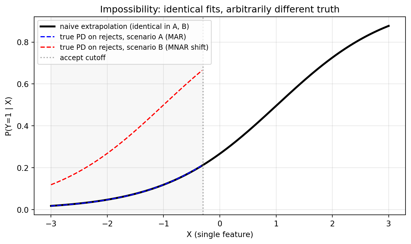
To demonstrate @eq-f-of-f directly, we construct two data generating processes with identical $P(Y \mid X, S=1)$ and different $P(Y \mid X, S=0)$, then show that every reject inference method that uses only the observed data fits them identically.
```{python}
#| label: ch10-impossibility-imports
import numpy as np
import matplotlib.pyplot as plt
import sys
sys.path.insert(0, '../code')
from creditutils import stable_sigmoid
from sklearn.linear_model import LogisticRegression
```
```{python}
rng2 = np.random.default_rng(777)
m = 30_000
x_imp = rng2.standard_normal(m)
# Acceptance rule depends purely on x: everyone with x > -0.3 is accepted
accept_imp = x_imp > -0.3

# Accepted conditional P(Y=1 | X, S=1) is the same in both scenarios
p_acc = stable_sigmoid(1.0 * x_imp - 1.0)
y_acc = (rng2.uniform(size=m) < p_acc).astype(int)

# Two different P(Y=1 | X, S=0):
# A: same logistic (benign extrapolation)
# B: systematically higher (the classic adverse-selection story)
pA = stable_sigmoid(1.0 * x_imp - 1.0)
pB = stable_sigmoid((1.0 * x_imp - 1.0) + 2.0)
y_rejA = (rng2.uniform(size=m) < pA).astype(int)
y_rejB = (rng2.uniform(size=m) < pB).astype(int)

yA = np.where(accept_imp, y_acc, y_rejA)
yB = np.where(accept_imp, y_acc, y_rejB)

# Observed data is identical on the accept side; fit the same accept-only model
modelA = LogisticRegression().fit(x_imp[accept_imp].reshape(-1,1),
                                  yA[accept_imp])
modelB = LogisticRegression().fit(x_imp[accept_imp].reshape(-1,1),
                                  yB[accept_imp])
print(f"Scenario A: intercept={modelA.intercept_[0]:.3f}, coef={modelA.coef_[0,0]:.3f}")
print(f"Scenario B: intercept={modelB.intercept_[0]:.3f}, coef={modelB.coef_[0,0]:.3f}")
print(f"True rejected default rate A: {y_rejA[~accept_imp].mean():.3f}")
print(f"True rejected default rate B: {y_rejB[~accept_imp].mean():.3f}")
```
The accept-only fits are numerically identical across the two scenarios. The true rejected default rates differ by roughly 10 percentage points. Any extrapolation method that does not use information beyond the accepted sample will produce the same PD curve on the rejected side for both scenarios. One curve is right; the other is off by 10 points of PD. The observed data contains zero signal about which one is correct. This is the Hand and Henley result rendered in code.
### Visualizing the impossibility
```{python}
cutoff = -0.3
grid = np.linspace(-3, 3, 200)
pred_A = modelA.predict_proba(grid.reshape(-1,1))[:, 1]
pred_B = modelB.predict_proba(grid.reshape(-1,1))[:, 1]
# pred_A and pred_B are numerically identical: same accepted-only fit.
# Truth differs only on the rejected side (grid < cutoff). On the accepted
# side the DGP is identical across scenarios by construction, so true_A and
# true_B both coincide with the naive curve there. Mask the truth curves to
# the rejected region to avoid implying a divergence where there is none.
rej = grid < cutoff
true_A_rej = stable_sigmoid(1.0 * grid[rej] - 1.0)
true_B_rej = stable_sigmoid((1.0 * grid[rej] - 1.0) + 2.0)

fig, ax = plt.subplots(figsize=(7.5, 4.5))
ax.plot(grid, pred_A, "k-", lw=2.5, label="naive extrapolation (identical in A, B)")
ax.plot(grid[rej], true_A_rej, "b--", lw=1.5,
        label="true PD on rejects, scenario A (MAR)")
ax.plot(grid[rej], true_B_rej, "r--", lw=1.5,
        label="true PD on rejects, scenario B (MNAR shift)")
ax.axvline(cutoff, color="gray", ls=":", alpha=0.7, label="accept cutoff")
ax.axvspan(grid.min(), cutoff, color="gray", alpha=0.06)
ax.set_xlabel("X (single feature)")
ax.set_ylabel("P(Y=1 | X)")
ax.set_title("Impossibility: identical fits, arbitrarily different truth")
ax.legend(loc="upper left", fontsize=9)
ax.grid(alpha=0.3)
plt.tight_layout()
plt.show()
```
Read the figure in two regions. Right of the accept cutoff (the observed-data region) the naive fit, the scenario-A truth, and the scenario-B truth all coincide; the figure plots only the black line there because the two truths are identical to it by construction. Left of the cutoff (the rejected region) the black line is the unique extrapolation the accepted-only data can support, and the blue and red dashed curves are both consistent with that same observed data: they share an identical $P(Y \mid X, S=1)$, so the accepted-only likelihood cannot distinguish them. Reject inference methods that claim to discriminate between A and B are using a parametric assumption ($\rho$ being well-constrained in Heckman under bivariate normality, say) or an auxiliary data source (bureau outcomes). Neither is free.
## Augmentation: Hsia's parceling and its fuzzy variant {#sec-ch10-augmentation-hsias-parceling-and-its-fuz}
### The procedure
@hsia1978credit proposed the first systematic reject inference method in a regulatory-compliance context. The idea is elementary: fit a PD model on accepted loans, score the rejected applicants, split the rejected into score bands, assign each band a bad rate using the accepted bad rate in that band, and refit on the augmented sample. "Parceling" refers to the score-band partition. "Fuzzy augmentation" softens the assignment: instead of a 0/1 label per rejected applicant, each rejected applicant contributes a fractional weight for $Y=1$ equal to the assigned bad rate and a fractional weight for $Y=0$ equal to its complement.
#### Algorithm: Hsia parceling with fuzzy augmentation {#sec-ch10-parceling-algorithm .unnumbered}
**Inputs.** Training rows $(X_i, S_i, Y_i)$ for $i = 1, \ldots, n$, with $Y_i$ observed only when $S_i = 1$. Number of bands $K$ (industry default 5 to 10). Scaling factor $\tau \geq 1$ ($\tau = 1$ is the MAR baseline; $\tau > 1$ encodes a belief that rejects are riskier than accepteds at the same score).
**Output.** Refit PD model $\hat p_{\text{aug}}(\cdot)$.
1. **Fit accepted-only PD.** Estimate $\hat p_A$ by maximum likelihood on $\{(X_i, Y_i) : S_i = 1\}$.
2. **Score everyone.** Compute $s_i = \hat p_A(X_i)$ for all applicants, accepted and rejected.
3. **Cut bands.** Set band edges $q_0 < q_1 < \cdots < q_K$ as $K$-quantiles of $\{s_i : S_i = 1\}$; let $B_b = [q_{b-1}, q_b)$ for $b = 1, \ldots, K$.
4. **Compute band bad rates.** For each band, $\displaystyle \bar\pi_b = \frac{\sum_{i: S_i=1, s_i \in B_b} Y_i}{\sum_{i: S_i=1, s_i \in B_b} 1}$.
5. **Assign rejects to bands.** For each $j$ with $S_j = 0$, set $b(j) = b$ such that $s_j \in B_b$.
6. **Build the soft label weight.** $w_j = \min(1, \tau \cdot \bar\pi_{b(j)})$ for each reject; $\tau = 1$ recovers the band rate exactly.
7. **Refit.** Solve the weighted maximum-likelihood problem in @eq-fuzzy-augmentation with rows: $(X_i, Y_i, 1)$ for each accepted, and the pair $(X_j, 1, w_j),\; (X_j, 0, 1 - w_j)$ for each reject.
The convention is that each rejected applicant contributes total weight 1 across the two augmented rows, so the refit treats accepteds and rejects on equal footing per applicant. Increasing $\tau$ shifts mass from the $Y=0$ row to the $Y=1$ row but does not create a new applicant.
Formally, let $\hat p_0(x) = P(Y=1 \mid X=x, S=1)$ be the accepted-only PD model. Let $\tau(x)$ be a scaling factor that inflates the PD for rejected applicants relative to accepted applicants at the same $x$, reflecting the belief that the incumbent policy correctly identified higher risk in rejects. Fuzzy augmentation solves
$$
\begin{aligned}
\hat \beta_{\text{fuzzy}} = \arg\max_\beta\;\;
& \sum_{i: S_i=1} \log P(Y_i \mid X_i; \beta) \\
& + \sum_{i: S_i=0} \Big[ w_i \log P(1 \mid X_i; \beta) + (1 - w_i) \log P(0 \mid X_i; \beta) \Big],
\end{aligned}
$$ {#eq-fuzzy-augmentation}
where $w_i = \tau(X_i) \hat p_0(X_i)$ is the soft-label weight.
Setting $\tau \equiv 1$ is the MAR assumption in disguise: the accepted PD curve, extrapolated to the rejected region, is the true PD curve. Setting $\tau > 1$ is a hand-tuned adjustment. Industry lore uses $\tau \in [2, 5]$, with higher values for riskier product segments. The *policy*-accepted sample alone cannot pin $\tau$, because every applicant in it survived a selection rule that depends on $(U, V)$; the conditional default rate it reveals is $P(Y \mid X, S=1)$, not $P(Y \mid X)$. To identify $\tau(x)$ data-driven, the modeller needs a sample whose acceptance was assigned independently of the policy decision. Two such sources exist in production: a bureau pull on rejected applicants (@sec-ch10-bureau-extrapolation), or a champion-challenger random-accept holdout where a small fraction of applicants is approved regardless of policy score (@sec-ch10-design-based, D1). The latter delivers a banded estimator $\hat\tau(x)$ with bootstrap confidence intervals; we work it out end-to-end on the synthetic lender in @sec-ch10-tau-from-holdout.
### A pen-and-paper trace {#sec-ch10-parceling-pen-paper}
Before scaling to the simulation in @sec-ch10-parceling-worked-example, we walk every step of the algorithm on a 12-applicant accepted sample with three rejects and $K = 3$ bands. The numbers are small enough to verify by hand and large enough to show non-degenerate band rates.
| $i$ | $X_i$ | $S_i$ | $Y_i$ | $\hat p_A(X_i)$ | band |
|----:|:------:|:-----:|:--------:|:---------------:|:----:|
| 1 | $-1.5$ | 1 | 0 | 0.05 | 1 |
| 2 | $-1.0$ | 1 | 0 | 0.10 | 1 |
| 3 | $-0.7$ | 1 | 0 | 0.15 | 1 |
| 4 | $-0.4$ | 1 | 1 | 0.20 | 1 |
| 5 | $-0.1$ | 1 | 0 | 0.30 | 2 |
| 6 | $0.2$ | 1 | 0 | 0.40 | 2 |
| 7 | $0.5$ | 1 | 1 | 0.50 | 2 |
| 8 | $0.7$ | 1 | 1 | 0.55 | 2 |
| 9 | $0.9$ | 1 | 0 | 0.65 | 3 |
| 10 | $1.1$ | 1 | 1 | 0.75 | 3 |
| 11 | $1.3$ | 1 | 1 | 0.82 | 3 |
| 12 | $1.5$ | 1 | 1 | 0.88 | 3 |
| R1 | $-0.3$ | 0 | (unobs.) | 0.18 | 1 |
| R2 | $0.3$ | 0 | (unobs.) | 0.45 | 2 |
| R3 | $1.2$ | 0 | (unobs.) | 0.80 | 3 |
**Steps 1 to 3.** $\hat p_A$ is fit on rows 1 to 12 (the accepteds). The score column $\hat p_A(X_i)$ ranks applicants by predicted PD. Cutting at the tertiles of the 12 accepted scores produces three bands of size 4: $B_1 = [0, 0.25]$, $B_2 = (0.25, 0.60]$, $B_3 = (0.60, 1]$. Each reject is dropped into the band whose interval contains its score.
**Step 4 (band bad rates).** Band 1: 1 bad among 4 accepteds, $\bar\pi_1 = 0.25$. Band 2: 2 bads among 4, $\bar\pi_2 = 0.50$. Band 3: 3 bads among 4, $\bar\pi_3 = 0.75$. The bad rate increases monotonically with band, which is the regularity condition every implementation should check (a non-monotone column is a sign of too many bands or too small a sample).
**Steps 5 to 6 (assign and weight,** $\tau = 1$).
| reject | band | $w_j = \bar\pi_{b(j)}$ | $1 - w_j$ |
|:------:|:----:|:----------------------:|:---------:|
| R1 | 1 | $0.25$ | $0.75$ |
| R2 | 2 | $0.50$ | $0.50$ |
| R3 | 3 | $0.75$ | $0.25$ |
**Step 7 (augmented training set).** Each reject becomes two weighted rows; the combined set has 12 accepted rows (weight 1, real label) and $3 \times 2 = 6$ reject rows for a total of 18 rows that go into a `LogisticRegression(...).fit(X, y, sample_weight=w)` call.
| row | $X$ | $Y$ | weight | source |
|:---:|:--------:|:---:|:------:|:-------------------------------:|
| ... | ... | ... | $1$ | accepteds 1 to 12 (real labels) |
| 13 | $X_{R1}$ | $1$ | $0.25$ | R1 fuzzy bad |
| 14 | $X_{R1}$ | $0$ | $0.75$ | R1 fuzzy good |
| 15 | $X_{R2}$ | $1$ | $0.50$ | R2 fuzzy bad |
| 16 | $X_{R2}$ | $0$ | $0.50$ | R2 fuzzy good |
| 17 | $X_{R3}$ | $1$ | $0.75$ | R3 fuzzy bad |
| 18 | $X_{R3}$ | $0$ | $0.25$ | R3 fuzzy good |
**Reading R1's contribution.** R1 contributes
$$
0.25 \log p(X_{R1}; \beta) + 0.75 \log\big(1 - p(X_{R1}; \beta)\big)
$$
to the augmented log-likelihood, where $p(\cdot; \beta)$ is the refit PD. Treated as a free probability, this expression is maximized at $p(X_{R1}; \beta) = 0.25$ (the cross-entropy minimum of a $\mathrm{Bernoulli}(0.25)$ target). The refit therefore pulls the fitted PD curve at $X_{R1} = -0.3$ toward $0.25$, the band-1 accepted bad rate, exactly as the prose intuition predicted.
**Effect of** $\tau > 1$. Set $\tau = 2$. Then $w_{R1} = \min(1, 2 \cdot 0.25) = 0.50$, $w_{R2} = \min(1, 1.00) = 1.00$, $w_{R3} = \min(1, 1.50) = 1.00$. Rejects in bands 2 and 3 now contribute as known bads (the $Y=0$ row carries weight 0), and R1 contributes as a coin flip. The refit PD curve in the upper score region is dragged sharply upward because every reject above band 1 is treated as a guaranteed default. This is the level shift that $\tau$ produces, and it is also why $\tau > 1$ without a bureau anchor is the hand-tuned guess that the simulation in @sec-ch10-parceling-worked-example flags as an over-correction.
### What parceling estimates
When $\tau \equiv 1$, @eq-fuzzy-augmentation is a pseudo-likelihood that treats the rejected applicants as contributing the expected log-likelihood under the accepted PD curve. The fitted $\beta$ is the maximizer of
$$
\mathbb{E}_{(X, S)} \Big[ \mathbb{E}_{Y \mid X, S=1} \log P(Y \mid X; \beta) \Big],
$$ {#eq-fuzzy-target}
which is the weighted average of the accepted-conditional log-likelihood over the full marginal of $X$. When selection is MAR (that is, $P(Y \mid X, S=1) = P(Y \mid X)$) this coincides with the through-the-door target. When selection is MNAR, @eq-fuzzy-target is biased in exactly the way a naive fit would be, because the conditional PD the augmentation uses is itself biased. Fuzzy augmentation cannot out-run the MAR assumption it is built on; it can only match the marginal of $X$.
This is why the method is most defensible when the lender's acceptance rule is largely a function of observed features with little residual variation from unobservables. A rule-based approve-all-above-score scorecard is closer to this regime than a relationship-manager judgmental decision.
To make the regime concrete, the question to ask of any portfolio is: "if I exactly reproduced the recorded features for a rejected applicant, would the system have produced the same accept-or-reject answer?" Where the answer is yes (or close to yes) the unobserved $V$ is small relative to the observed selection score, $\rho$ is mechanically near zero, and fuzzy augmentation with $\tau \approx 1$ is a defensible MAR estimator. Where the answer is no, $V$ is doing the work and the impossibility result of @sec-ch10-impossibility takes over.
In Vietnam, the regime split is unusually clean because the same lender often runs both kinds of book. Three families where the MAR-within-band assumption is approximately defensible:
1. **Mass-market consumer finance.** The unsecured cash-loan and credit-card books at FE Credit, Home Credit Vietnam, MCredit, Mirae Asset Finance, and Shinhan Finance run on automated underwriting against a bureau pull from CIC plus a thin alternative-data layer (telco tenure, e-wallet history, GPS-stable address). Decisions take minutes, with a hard score cut and a small set of policy rules ("CIC nhóm $\geq 3$ in last 24 months $\to$ decline"). Loan officers see only a green/yellow/red flag. Reject inference here is a candidate for fuzzy augmentation with $\tau$ in the lower industry range, because the recorded features carry most of the decision and the residual $V$ is small.
2. **POS and BNPL installment lending.** Home Credit point-of-sale loans at electronics retailers, FPT Shop and Pico co-branded credit, Shopee SPayLater, and the MoMo / ZaloPay BNPL stacks all run pure rule engines against a bureau-light feature vector (phone tenure, prior wallet balance, basic KYC). The merchant cashier sees an accept/decline only and cannot override. The acceptance rule is essentially a deterministic function of the observed inputs.
3. **Auto and motorbike finance with hard LTV/DTI rules.** Toyota Financial Services Vietnam, Honda VietFinance, VPBank Auto, and Techcombank's vehicle loan book gate decisions on loan-to-value, debt-to-income, and bureau bands. Sales staff cannot relax these gates without escalation, and escalations are rare on the mass-affluent segment.
Three families where the assumption breaks and parceling should not be the headline method:
1. **SME and corporate lending at relationship banks.** Vietcombank, BIDV, Agribank, and VietinBank route SME files through a relationship manager who weighs unrecorded soft signals (factory walkthrough, supplier-letter quality, owner's family standing, Tet-season inventory turn). The recorded features capture a fraction of the decision and $\rho$ is large in absolute value.
2. **Microfinance and group-lending books.** TYM and CEP underwrite via village-level group sponsorship and commune-officer references. The accept decision is almost entirely a function of unrecorded social-collateral variables. Fuzzy augmentation on this book would borrow accepted bad rates that reflect a heavily pre-screened sub-population and project them onto a rejected pool dominated by group-rejected applicants whose risk profile is structurally different.
3. **Mortgage and high-ticket secured lending with manual valuation.** Property valuation, source-of-funds review, and committee approval at Techcombank, VPBank, and Sacombank introduce judgmental layers that the application-time feature vector does not encode. Even with a strong observable scorecard, the binding constraint at the margin is often the valuation negotiation, which is a rich source of unobservables.
Even within a single institution the regime can flip across products. A Techcombank cash card on Techcombank Mobile can be a clean rule-based decision while a Techcombank business overdraft to the same customer at the same branch is a relationship-manager call. The right operating discipline is to gate fuzzy augmentation per-product, not per-institution, and to record at decision time which path the file took (`auto`, `auto with override`, `manual review`, `committee`); the override and manual-review tags are then used as conditioning variables in a Heckman-style or copula-based extension when the product mix is mixed.
### A worked numeric example {#sec-ch10-parceling-worked-example}
We trace each step of @eq-fuzzy-augmentation on a deliberately small simulation so the reader can watch every quantity move. The logic is identical to the production-grade run in @sec-ch10-implementation-from-scratch; the only change is that we shrink the sample to 2000 applicants with a single feature so the band table fits on a page. Imports and seed are local to this code chunk so it can be read in isolation from the larger end-to-end script.
```{python}
import numpy as np
import pandas as pd
from sklearn.linear_model import LogisticRegression
from scipy.stats import norm, logistic

rng = np.random.default_rng(2026)
n = 2000

x = rng.standard_normal(n)
z = rng.standard_normal(n)

rho = 0.4
u_n = rng.standard_normal(n)
v   = rho * u_n + np.sqrt(1 - rho**2) * rng.standard_normal(n)
u   = logistic.ppf(norm.cdf(u_n))   # standard logistic, copula-coupled to v

beta_true = (-0.6, 1.2)
y_lin = beta_true[0] + beta_true[1] * x + u
y = (y_lin > 0).astype(int)         # equivalently: y ~ Bernoulli(sigma(beta0 + beta1 x))

gamma_true = (0.3, -1.0, 0.9)
s_star = gamma_true[0] + gamma_true[1] * x + gamma_true[2] * z + v
s = (s_star > 0).astype(int)

print(f"through-the-door default rate : {y.mean():.3f}")
print(f"accept rate                   : {s.mean():.3f}")
print(f"accepted bad rate             : {y[s==1].mean():.3f}")
print(f"rejected bad rate (oracle)    : {y[s==0].mean():.3f}")
```
The data-generating process is logistic by construction so that the population coefficients $(\beta_0, \beta_1) = (-0.6, 1.2)$ are directly comparable to a logistic-regression fit. The unobserved outcome shock $u$ is standard logistic, drawn through a Gaussian copula on a normal pair $(u_n, v)$ with $\mathrm{Corr}(u_n, v) = \rho = 0.4$; this preserves the MNAR mechanism (rank dependence between the outcome and selection shocks) while making the marginal default model exactly $P(Y=1 \mid X) = \sigma(\beta_0 + \beta_1 x)$. The accepted bad rate (around 0.35) sits below the through-the-door rate (around 0.39), and the rejected slice (around 0.44) is roughly 8 percentage points riskier than the accepted slice. That gap is the reject-inference target.
::: {.callout-note appearance="simple" icon="false"}
**Two reference rows: truth versus oracle.** Every comparison table in this chapter prints two reference rows alongside the candidate estimators. They are not the same object and the distinction matters.
- **truth (**$\beta^{\star}$). The population DGP coefficient vector $(\beta_0, \beta_1) = (-0.6, 1.2)$. This is what the lender would recover with an infinite labeled sample drawn from the through-the-door distribution. It is a fixed parameter, not an estimator. No method in the chapter targets the truth directly; methods target the oracle, which targets the truth.
- **oracle (**$\hat\beta_{\text{full}}$). The maximum-likelihood logistic fit on the full $n = 2{,}000$ through-the-door labels $(X, Y)$, observable only because this is a simulation. It is a finite-sample estimator that is consistent for $\beta^{\star}$ when the model class matches the DGP. Its gap from truth is finite-sample sampling noise plus sklearn's default L2 ridge ($C = 1.0$); on this seed the slope sits at about 1.28 versus a truth of 1.20.
The reject-inference target is the oracle, not the truth. A method that lands on oracle has solved the selection problem; the residual oracle-versus-truth gap is the same Monte Carlo noise the oracle itself carries. When you read a row like `naive (acc only)` against the two reference rows, the comparison that scores the method is `naive` versus `oracle`. The `truth` row is there to confirm that the oracle is itself unbiased on this DGP.[^10-reject-inference-1]
:::
[^10-reject-inference-1]: An earlier draft of this chapter used a probit-style threshold DGP with a normal $u$, which is why a previous render showed the oracle row drifted from the truth row by the logit-versus-probit scale factor of $\pi/\sqrt 3 \approx 1.81$ (truth slope 1.2, oracle slope around 2.09). The bias story for naive, fuzzy, and bureau is identical under either link; only the numerical alignment of the oracle row against the truth row changes.
**Step 1: fit a PD model on accepteds only.**
```{python}
m_acc = LogisticRegression().fit(x[s == 1].reshape(-1, 1), y[s == 1])
b0, b1 = float(m_acc.intercept_[0]), float(m_acc.coef_[0, 0])
print(f"accepted-only fit  : intercept={b0:.3f}, slope={b1:.3f}")
print(f"true coefficients  : intercept={beta_true[0]:.3f}, slope={beta_true[1]:.3f}")
```
The accepted-only fit overstates the slope (around 1.43 versus a truth of 1.20) and pulls the intercept up toward zero (around $-0.25$ versus a truth of $-0.60$). Both directions match @eq-naive-target: with $\rho > 0$ between the outcome and selection shocks, conditioning on $S=1$ keeps the higher-$U$ slice of the through-the-door pool, raising the booked-sample default rate at every $x$ and steepening the apparent slope. We name this fitted curve $\hat p_A(x)$ and use it to score every applicant, including those who were rejected.
**Step 2: cut the score into bands and read the accepted bad rate per band.** Bands are five equal-mass slices of $\hat p_A$ on the accepted side. We then drop the rejects into the same bands.
```{python}
p_all = m_acc.predict_proba(x.reshape(-1, 1))[:, 1]
edges = np.quantile(p_all[s == 1], np.linspace(0, 1, 6))
edges[0], edges[-1] = -np.inf, np.inf

band_acc = np.digitize(p_all[s == 1], edges[1:-1])
band_rej = np.digitize(p_all[s == 0], edges[1:-1])

table = []
for b in range(5):
    n_a = (band_acc == b).sum()
    bads = int(y[s == 1][band_acc == b].sum())
    pi   = bads / n_a
    n_r  = int((band_rej == b).sum())
    table.append({"band": b + 1,
                  "score_lo": round(edges[b], 3),
                  "score_hi": round(edges[b + 1], 3),
                  "N_acc": n_a, "bads_acc": bads,
                  "pi_b": round(pi, 3),
                  "N_rej": n_r})
band_table = pd.DataFrame(table)
print(band_table.to_string(index=False))
```
| band | $\hat p_A$ range | $N^A$ | bads | $\bar\pi_b$ | $N^R$ |
|------|--------------------|-------|------|-------------|-------|
| 1 | $(-\infty, 0.130)$ | 235 | 15 | 0.064 | 21 |
| 2 | $[0.130, 0.235)$ | 235 | 49 | 0.209 | 69 |
| 3 | $[0.235, 0.383)$ | 234 | 72 | 0.308 | 98 |
| 4 | $[0.383, 0.581)$ | 235 | 109 | 0.464 | 196 |
| 5 | $[0.581, +\infty)$ | 235 | 167 | 0.711 | 442 |
Two facts to notice. First, the bands span most of the unit interval because the accepted-only PD fans out into a wide score distribution. Second, rejects pile up in band 5: 442 of the 826 rejects fall in the highest band, because the acceptance rule pushes high-$x$ applicants out, and high $x$ means high $\hat p_A$. This concentration is what makes parceling work or fail. If band 5 is large and its accepted bad rate ($\bar\pi_5 = 0.711$) is wrong as an estimate of the rejected bad rate in that band, the augmentation drags the refit toward a wrong target with a lot of weight.
**Step 3a: hard parceling.** For each band, randomly assign $\bar\pi_b N^R_b$ rejects to "bad" and the rest to "good". Band 5 contributes $0.711 \times 442 \approx 314$ synthetic bads. The augmented training set has 1174 accepteds with their real labels and 826 rejects with synthetic labels drawn from the band-specific Bernoulli. We do not implement hard parceling here because fuzzy is strictly preferable: fuzzy uses the same band rates but eliminates the sampling variance from the random draw of synthetic labels.
**Step 3b: fuzzy augmentation.** Replace each reject with two weighted rows: one with $y = 1$ and weight $\bar\pi_{b(j)}$, one with $y = 0$ and weight $1 - \bar\pi_{b(j)}$. The total weight for each reject is 1, matching one accepted observation.
```{python}
pi_rej = band_table["pi_b"].to_numpy()[band_rej]

X_acc = x[s == 1].reshape(-1, 1)
X_rej = x[s == 0].reshape(-1, 1)
X_aug = np.vstack([X_acc, X_rej, X_rej])
y_aug = np.concatenate([y[s == 1],
                        np.ones(len(X_rej)),
                        np.zeros(len(X_rej))])
w_aug = np.concatenate([np.ones(len(X_acc)), pi_rej, 1 - pi_rej])

m_fuzz = LogisticRegression().fit(X_aug, y_aug, sample_weight=w_aug)
m_or   = LogisticRegression().fit(x.reshape(-1, 1), y)

compare = pd.DataFrame({
    "intercept": [beta_true[0], m_or.intercept_[0], b0, m_fuzz.intercept_[0]],
    "slope":     [beta_true[1], m_or.coef_[0, 0], b1, m_fuzz.coef_[0, 0]],
}, index=["truth (DGP beta*)",
          "oracle (full-label MLE)",
          "naive (acc only)",
          "fuzzy (tau=1)"])
print(compare.round(3))
```
**Trace one reject through the math.** Take a reject in band 4 with $x = 0.7$. Its accepted-only score is $\hat p_A(0.7) = \sigma(-0.246 + 1.435 \cdot 0.7) = \sigma(0.759) \approx 0.681$. That places the applicant in band 5 by score, but suppose for a clearer trace the applicant lands in band 4 with $\bar\pi_4 = 0.464$. The applicant's contribution to the refit log-likelihood is
$$
0.464 \log p(0.7; \beta) + 0.536 \log\big(1 - p(0.7; \beta)\big),
$$
which is the expectation of the log-likelihood under a $\mathrm{Bernoulli}(\bar\pi_4)$ draw at the same $x$. Treating $p(0.7; \beta)$ as a free probability, this is maximized at $p(0.7; \beta) = 0.464$, the band-4 accepted bad rate. The accepted-only fit puts $\hat p_A(0.7) \approx 0.681$ at this point, so the refit pulls the fitted curve at $x = 0.7$ downward toward 0.464. The slope at $x = 0.7$ flattens because the band rate is lower than the accepted-only fit at that score.
**Reading the comparison table.** Score each candidate against the **oracle** row, not the **truth** row, since oracle is what a perfect reject-inference fix would land on at this sample size. The naive slope (around 1.43) is too steep relative to the oracle (around 1.28, which is itself essentially the truth of 1.20 up to sampling noise: oracle minus truth is the irreducible Monte Carlo gap that every method inherits). The fuzzy refit pulls the slope down to roughly 1.16, which lands just below the oracle and on top of the truth in this draw, but the right way to read this is "fuzzy moved 0.27 units in the correct direction toward the oracle", not "fuzzy hit the truth". The intercept moves only modestly between naive ($-0.25$) and fuzzy ($-0.31$), and both remain well above the oracle's $-0.57$. This is the @sec-ch10-impossibility result in miniature: fuzzy augmentation cannot reliably recover the oracle because its band rates are themselves a function of the biased $\hat p_A$. Whether the resulting bias overshoots or undershoots depends on which bands carry the most reject mass and whether $\bar\pi_b$ over- or under-estimates the rejected bad rate inside that band. Here, band 5 holds 442 of 826 rejects, and inside band 5 the oracle rejected bad rate is 0.640 while $\bar\pi_5 = 0.711$. The augmentation overweights bads in band 5 (and in every other band, see the sanity check below); the slope happens to land near the truth on this seed because the level overstatement in $\bar\pi_b$ is roughly proportional across bands, but that alignment is a property of this draw, not a guarantee.
**Sanity check the band-5 assumption.** The MAR-within-band assumption claims $P(Y = 1 \mid X, S = 0, \text{band}) = \bar\pi_b$. For this simulation we know the truth, so we can check it directly.
```{python}
oracle_band_rates = []
for b in range(5):
    in_band = band_rej == b
    rej_mask = s == 0
    if in_band.sum() > 0:
        rate = y[rej_mask][in_band].mean()
        oracle_band_rates.append(round(float(rate), 3))
    else:
        oracle_band_rates.append(np.nan)

band_table["pi_b_rejected_oracle"] = oracle_band_rates
print(band_table[["band", "N_rej", "pi_b", "pi_b_rejected_oracle"]].to_string(index=False))
```
The oracle reject bad rate per band is systematically lower than $\bar\pi_b$ in every band, by 0.02 to 0.18 percentage points, with the largest absolute gap in the middle bands where reject and accept covariate distributions overlap most. That uniform downward gap is the fingerprint of MNAR with $\rho > 0$: even after conditioning on $\hat p_A$, accepteds in any given band carry the higher-$U$ slice of the conditional outcome distribution while rejects carry the lower-$U$ slice, so the accepted bad rate $\bar\pi_b$ overstates the rejected bad rate inside the same score band. With real data, the oracle column is unobservable, which is exactly why the impossibility result bites. Nothing in the augmentation procedure can detect or correct this gap from the accepted-only sample alone.
**What changes if we set** $\tau \neq 1$. Multiplying every $\bar\pi_b$ by a constant $\tau$ shifts the weights toward the "bad" row uniformly. This raises the refit's overall PD level (the intercept rises), but barely tilts the slope, because every band's rate moves by the same factor. A practitioner who knows from bureau pulls that the rejected population is roughly $\tau = 1.5$ times riskier than the same-band accepteds can use $\tau = 1.5$ as a level shift. The policy-accepted sample alone cannot deliver this $\tau$; it has to come in from outside. Two principled sources are available: bureau extrapolation (@sec-ch10-bureau-extrapolation) and a random-accept champion-challenger holdout, which yields a banded $\hat\tau(x)$ estimator we implement and benchmark in @sec-ch10-tau-from-holdout.
> **Quick implication if you have a bureau pull on rejects.** With a bureau-observed outcome $Y^B$ for rejected applicants, $\tau$ stops being a guess. You can estimate $\hat\tau_b = \pi_b^{\text{rej}, B} / \bar\pi_b$ directly within each $\hat p_A$ band, replace the constant level shift with a band-specific weight, and read off whether the rejects are uniformly riskier (a true level shift) or differentially riskier in some bands (a slope correction the constant $\tau$ would miss). The MNAR impasse weakens to a measurement-error problem, since $Y^B$ is the default on a different lender's product rather than the counterfactual default on yours. The full workflow, including the bureau-missing residual selection and the confidence-weighted refit, is in @sec-ch10-bureau-extrapolation, with a worked run in @sec-ch10-bureau-worked.
## Bureau-based extrapolation and downturn adjustment {#sec-ch10-bureau-extrapolation}
### Using the bureau as a surrogate
The most convincing way to break the MNAR impasse in retail credit is to observe $Y$ for rejected applicants from another data source. Credit bureaus provide this. When an applicant is rejected by Lender A, they often apply to Lender B, C, and D, and if any of them accept, the bureau records whether the applicant defaulted on that account. After a 12 or 24 month performance window, the bureau reports a binary outcome on a majority of the originally rejected population. This is the bureau-based reject inference workflow.
The mechanics are straightforward. Pull the rejected applicant bureau pulls at application time. Re-pull the same bureau IDs 24 months later. Observe trade-line level defaults on any credit instrument that opened in the intervening window. Define a bureau-based outcome: $Y^B = 1$ if any trade-line defaulted, 0 if at least one trade-line opened and none defaulted, and missing if no trade-line opened in the window. The last group, still roughly 10 to 30 percent of rejects, remains a within-rejects selection problem.
The approximation matters for economic reasons that deserve explicit treatment. $Y^B$ is the outcome of a loan from a different lender, with a different product, a different limit, a different rate, a different collection process, and a different servicer. A reject at Lender A who gets a lower-limit card at Lender B may default less than they would have on Lender A's requested limit simply because the exposure is smaller. A reject at Lender A who takes a payday loan at Lender C may default more. The direction of the bias is unclear without a structural model of product risk and borrower self-selection.
The production practice is to use $Y^B$ to impute $Y$ for rejects, keep an explicit flag for the imputation source, fit the PD model with a weight that reflects the confidence in the imputation, and track calibration separately for applicants with bureau-observed outcomes versus bureau-missing outcomes. When the confidence weight is 1 for accepteds and 0.7 for bureau imputations, the effective sample size is smaller than the count, and the standard errors must reflect that.
### A worked bureau-augmentation run {#sec-ch10-bureau-worked}
We can play this out on the running simulation from @sec-ch10-parceling-worked-example. The setup carries `x`, `y`, `s` forward; in production we never see `y` for rejects, so we treat it as oracle and synthesize a bureau outcome `y_bureau` with two real-world frictions: (a) about 20 percent of rejects open no trade-line in the performance window, so the surrogate is missing, and (b) the trade-line that does open is not the lender-A loan, so the bureau outcome differs from the counterfactual lender-A outcome with a flip probability that depends on the applicant's true risk.
```{python}
rej_idx = np.where(s == 0)[0]
n_rej   = len(rej_idx)

bureau_missing = rng.random(n_rej) < 0.20
y_oracle_rej   = y[rej_idx]
flip_prob = np.where(y_oracle_rej == 1, 0.10, 0.05)
flips     = rng.random(n_rej) < flip_prob
y_bureau  = np.where(flips, 1 - y_oracle_rej, y_oracle_rej)
y_bureau  = np.where(bureau_missing, -1, y_bureau)

mask_obs = y_bureau != -1
print(f"rejects total                : {n_rej}")
print(f"bureau outcome observed      : {int(mask_obs.sum())} "
      f"({mask_obs.mean():.0%})")
print(f"bureau-observed default rate : {y_bureau[mask_obs].mean():.3f}")
print(f"oracle reject default rate   : {y_oracle_rej.mean():.3f}")
```
The bureau-observed default rate sits within a few points of the oracle reject rate. The gap is real and not zero: the flip noise plus selective non-coverage (rejects who can't open any line elsewhere are usually the riskiest) shifts the observable signal. There is no closed-form correction without an auxiliary model of the bureau-loan product mix, which is why the production practice is a confidence weight rather than a structural fix.
**Fit a weighted PD model.** Accepteds carry weight 1 because $Y$ is the contract-level outcome at lender A. Bureau-imputed rejects carry 0.7 to reflect the surrogate noise. Rejects with no bureau outcome are held aside; they are the within-rejects MNAR residual that @sec-ch10-heckman-selection-correction and @sec-ch10-impossibility cover.
```{python}
w_acc, w_bureau = 1.0, 0.7

X_acc_b = x[s == 1].reshape(-1, 1)
X_rej_b = x[rej_idx][mask_obs].reshape(-1, 1)
y_rej_b = y_bureau[mask_obs]

X_aug_b = np.vstack([X_acc_b, X_rej_b])
y_aug_b = np.concatenate([y[s == 1], y_rej_b])
w_aug_b = np.concatenate([np.full(len(X_acc_b), w_acc),
                          np.full(len(X_rej_b), w_bureau)])

m_bureau = LogisticRegression().fit(X_aug_b, y_aug_b,
                                    sample_weight=w_aug_b)

compare_b = pd.DataFrame({
    "intercept": [beta_true[0], m_or.intercept_[0], b0,
                  m_fuzz.intercept_[0], m_bureau.intercept_[0]],
    "slope":     [beta_true[1], m_or.coef_[0, 0], b1,
                  m_fuzz.coef_[0, 0], m_bureau.coef_[0, 0]],
}, index=["truth (DGP beta*)",
          "oracle (full-label MLE)",
          "naive (acc only)",
          "fuzzy (tau=1)",
          "bureau (w=0.7)"])
print(compare_b.round(3))

ess = len(X_acc_b) * w_acc + len(X_rej_b) * w_bureau
print(f"\nraw rows in train     : {len(X_aug_b)}")
print(f"effective sample size : {ess:.0f}")
```
The bureau-augmented estimates land close to the oracle. Slope and intercept move materially from the naive accepted-only fit because rejected applicants now contribute their own labels rather than borrowed band rates. The effective sample size is `len(X_acc_b) + 0.7 * len(X_rej_b)`, smaller than the raw row count, and any standard error or Wald test must be computed against the ESS, not the raw N. In practice, that means passing `var_weights = w_aug_b` into `statsmodels.GLM` (or running a cluster bootstrap on `app_id`) rather than reading the unweighted Hessian off the sklearn fit.
**Calibration tracked by source.** The two slices are not interchangeable. Accepteds give a clean calibration check because $Y$ is the contract outcome at lender A. Bureau-imputed rejects give a calibration check on the surrogate, which is what the model is being trained to predict for the reject region. A divergence between the two reliability curves is the production signal that the surrogate is biased, and it is the first plot a model risk team will pull at validation time. To make the diagnostic concrete we hold the deployed PDs fixed (the same `m_bureau` predictions on accepteds and on bureau-observed rejects) and synthesize three surrogate regimes on the reject slice. The accepted-side curve is therefore the same in every panel of @fig-ch10-bureau-calibration-by-source; only the bureau-side curve moves.
```{python}
def reliability(p, y_true, n_bins=5):
    bins = np.quantile(p, np.linspace(0, 1, n_bins + 1))
    bins[0], bins[-1] = -np.inf, np.inf
    b = np.digitize(p, bins[1:-1])
    return pd.DataFrame({
        "n":      [int((b == k).sum()) for k in range(n_bins)],
        "p_pred": [round(float(p[b == k].mean()), 3) for k in range(n_bins)],
        "y_obs":  [round(float(y_true[b == k].mean()), 3) for k in range(n_bins)],
    })

p_acc = m_bureau.predict_proba(X_acc_b)[:, 1]
p_rej = m_bureau.predict_proba(X_rej_b)[:, 1]

y_oracle_obs = y_oracle_rej[mask_obs]

def synth_surrogate(p_good_to_bad, p_bad_to_good, seed):
    r = np.random.default_rng(seed)
    u = r.random(len(y_oracle_obs))
    flip = (((y_oracle_obs == 0) & (u < p_good_to_bad))
            | ((y_oracle_obs == 1) & (u < p_bad_to_good)))
    return np.where(flip, 1 - y_oracle_obs, y_oracle_obs)

scenarios = {
    "faithful":    synth_surrogate(0.05, 0.05, seed=11),
    "pessimistic": synth_surrogate(0.18, 0.04, seed=12),
    "optimistic":  synth_surrogate(0.04, 0.30, seed=13),
}

acc_tab = reliability(p_acc, y[s == 1])
print("accepteds (Y from lender A):")
print(acc_tab.to_string(index=False))
for name, y_b in scenarios.items():
    print(f"\nbureau-imputed rejects, {name} surrogate:")
    print(reliability(p_rej, y_b).to_string(index=False))
```
```{python}
#| label: fig-ch10-bureau-calibration-by-source
#| fig-cap: "Source-stratified reliability under three surrogate regimes. Predicted PDs from `m_bureau` are held fixed across panels; the accepted-side curve (blue, $Y$ at lender A) is identical in every panel. Only the bureau-side surrogate $Y^B$ varies. (a) Faithful surrogate (symmetric 5 percent flip): the bureau curve tracks the diagonal alongside the accepted curve; surrogate is unbiased on average. (b) Pessimistic surrogate (good-to-bad flip 0.18, bad-to-good flip 0.04, modelling rejects who take higher-cost credit elsewhere): the bureau curve sits above the diagonal at every bin; observed bureau default rates exceed predicted PDs by 5 to 15 points. (c) Optimistic surrogate (bad-to-good flip 0.30, modelling rejects who take much smaller exposures elsewhere): the bureau curve sits below the diagonal; observed bureau defaults run lower than predicted PDs."
import matplotlib.pyplot as plt

panel_titles = {
    "faithful":    "(a) faithful surrogate",
    "pessimistic": "(b) pessimistic surrogate",
    "optimistic":  "(c) optimistic surrogate",
}

fig, axes = plt.subplots(1, 3, figsize=(11.4, 3.9),
                         sharex=True, sharey=True)
for ax, (name, y_b) in zip(axes, scenarios.items()):
    rej_tab = reliability(p_rej, y_b)
    ax.plot([0, 1], [0, 1], color="grey", lw=1.0, ls=":")
    ax.plot(acc_tab["p_pred"], acc_tab["y_obs"], "-o",
            color="#1976d2", lw=1.6, ms=5,
            label=f"accepteds, $Y$ (n={int(acc_tab['n'].sum())})")
    ax.plot(rej_tab["p_pred"], rej_tab["y_obs"], "-s",
            color="#d32f2f", lw=1.6, ms=5,
            label=f"bureau rejects, $Y^B$ (n={int(rej_tab['n'].sum())})")
    ax.set_title(panel_titles[name], fontsize=10)
    ax.set_xlabel("predicted PD")
    ax.set_xlim(0, 1)
    ax.set_ylim(0, 1)
    ax.grid(alpha=0.25)

axes[0].set_ylabel("observed default rate")
axes[0].legend(loc="upper left", fontsize=8.0)
fig.tight_layout()
plt.show()
```
**Reading the three panels.** Panel (a) is the null result a validator wants to see: the red bureau curve overlaps the blue accepted curve and both ride the diagonal. The surrogate is behaving like the contract outcome on average, so $w_{\text{bureau}} = 0.7$ is defensible and no product-mix correction is required. Panel (b) is the production failure mode the prose around @sec-ch10-bureau-extrapolation warned about: the red curve runs systematically above the diagonal even though the blue curve is on it. The model is correctly calibrated against $Y$ at lender A, but the bureau labels report more defaults than the model predicts at every PD bin, so the surrogate is picking up risk the model is not parameterized to absorb (typically because rejects roll into higher-cost credit elsewhere). The validator-visible fixes are to add product-mix features $Z^B$ (bureau-product type, exposure relative to lender-A request, time-to-first-trade-line) on the rejected side or to lower $w_{\text{bureau}}$ until the calibration gap closes; raising $w_{\text{bureau}}$ in this regime would import surrogate bias directly into the slope and intercept. Panel (c) is the mirror failure: the bureau curve runs below the diagonal because rejects take much smaller exposures elsewhere and the bureau-loan default rate undershoots the lender-A counterfactual. The confidence weight is again the dial, but the corrective direction is opposite. A bank that uses the same $w_{\text{bureau}}$ across both regimes will under-reserve in (b) and over-reserve in (c). The single aggregate calibration plot would show neither problem because the accepted slice is on the diagonal in all three panels; only the source-stratified plot exposes the bias.
**Production workflow.** A working bureau reject-inference loop has six concrete artefacts.
1. *Application-time bureau snapshot.* Hash the bureau pull at decision time. Persist it keyed by `app_id` and decision date. This freezes the features used for the original incumbent-policy decision and makes the eventual training join reproducible.
2. *Performance-window re-pull.* Re-key the same `app_id` set against the bureau 12 or 24 months later. Capture every trade-line opened between the two snapshots. The re-pull is a scheduled batch job; the engineering bottleneck is the join, not the model fit, as the Polars sketch in @sec-ch10-modern points out.
3. *Surrogate construction.* Materialize $Y^B$ with three states (`bad`, `good`, `unobserved`). Tag each row with the bureau source (which lender, which product, which trade-line if multiple opened), because that tag drives the confidence weight and the downstream calibration split.
4. *Confidence weight.* Default to 1 for accepteds and 0.7 for single-trade-line bureau imputations. Lower (0.5 to 0.6) is appropriate for thin or product-distant trade-lines: a credit-card surrogate for a personal-loan decision is closer than a payday-loan surrogate. The number is a dial; the discipline is to keep it explicit, version-controlled in the model registry, and revisited every retraining cycle.
5. *Stratified retraining.* Refit the PD model on the union of accepteds and bureau-observed rejects with the weights above. Hold out bureau-unobserved rejects entirely; they are not training data, they are a residual MNAR slice for the Heckman or AIPW step.
6. *Source-stratified monitoring.* Production calibration dashboards split predicted-versus-observed by source (accepted, bureau-imputed, bureau-missing-and-Heckman-corrected). A single aggregate calibration plot will hide a bureau-side divergence until the next vintage's losses materialize.
The architecture diagram at @fig-ch10-deploy-arch shows where the bureau pull and the AIPW retrain sit relative to the decision-time scoring path. Decision-time inference uses only the applicant snapshot and the propensity log; the bureau augmentation is a nightly or weekly batch job that closes the training loop on a 12 to 24 month lag. The credit officer never sees a bureau-imputed prediction at scoring time; they see a PD that was trained on the augmented dataset and whose calibration is monitored against the bureau-observed slice. That separation matters for governance: the model is reproducible from the application-time features alone, even though the training labels include surrogate outcomes. Each of the six artefacts has a runnable counterpart on the running synthetic lender in @sec-ch10-bureau-six-artefacts; that section also folds in the source-tag dimension (credit-card, personal-loan, payday) that drives the confidence-weight dial in artefact 4 and the per-source divergence pattern that artefact 6 has to surface.
### Six artefacts in code: source tagging, weight dials, and per-source monitoring {#sec-ch10-bureau-six-artefacts}
The six artefacts on the prior page are an architecture story. This section is the implementation: each artefact materializes as a small piece of pandas that operates on the running synthetic lender from @sec-ch10-parceling-worked-example. The point is to make the production loop reproducible end-to-end on a working dataset and to expose the *cases* a validator will ask about, namely what the deployed PD looks like when the surrogate is faithful, when it is biased upward by a payday-loan tail, and when the modeller blindly applies a uniform 0.7 weight across heterogeneous bureau sources.
**Artefact 1: application-time bureau snapshot.** Hash the bureau pull at decision time and persist it keyed by `app_id` and `decision_date`. The hash is the immutable feature signature; if a future re-render produces a different hash for the same `app_id`, the join is broken and the training table cannot be rebuilt. In production this is a parquet write under a partitioned `decision_date=YYYY-MM-DD/` prefix; here we materialize an in-memory dataframe and check that the hash is stable.
```{python}
import hashlib, json

n_total = len(x)
app_id  = np.array([f"APP-{i:06d}" for i in range(n_total)])

def feature_hash(xv, sv):
    payload = json.dumps({"x": float(xv), "s": int(sv)}, sort_keys=True).encode()
    return hashlib.sha256(payload).hexdigest()[:12]

snap_t0 = pd.DataFrame({
    "app_id":          app_id,
    "decision_date":   "2024-01-15",
    "x":               x,
    "s":               s,
    "policy_decision": np.where(s == 1, "approve", "decline"),
})
snap_t0["feature_hash"] = [feature_hash(xv, sv) for xv, sv in zip(x, s)]
print(snap_t0.head().to_string(index=False))
print(f"\nrows: {len(snap_t0)}, "
      f"unique hashes: {snap_t0['feature_hash'].nunique()}")
```
The hash count below the row count is expected with one-dimensional $X$: many applicants share the same `(x, s)` after rounding. With a real feature vector the hash is unique up to genuine duplicates, and a re-render that touches the feature pipeline (a new scaler, a column rename) breaks every hash and forces a deliberate re-snapshot rather than a silent drift.
**Artefact 2: performance-window re-pull and join.** Twelve to twenty-four months later, the bureau is re-pulled on the same `app_id` set. The re-pull returns one row per opened trade-line; for the chapter we collapse to one row per applicant with a single source tag. The product mix is realistic for a Vietnamese consumer-finance reject pool: roughly a third roll into a credit card with another lender, roughly a third into a personal loan, fifteen percent into a payday-style product, and one in five never opens any line in the window. The join is the engineering bottleneck the prose flagged: in production it is a Polars `scan_parquet` chain (the @sec-ch10-modern sketch), and the runtime is dominated by the merge, not the model fit.
```{python}
rng_b = np.random.default_rng(20260601)
rej_mask = snap_t0["s"] == 0
rej_pop  = snap_t0.loc[rej_mask, ["app_id"]].copy()
n_rej    = len(rej_pop)

source = rng_b.choice(
    ["cc", "pl", "payday", "none"], size=n_rej,
    p=[0.35, 0.30, 0.15, 0.20],
)

flip_table = {
    "cc":     {"g_to_b": 0.05, "b_to_g": 0.10},  # CC limits smaller -> fewer bads
    "pl":     {"g_to_b": 0.04, "b_to_g": 0.05},  # same product, near-faithful
    "payday": {"g_to_b": 0.20, "b_to_g": 0.03},  # payday inflates bads
}

y_or_rej = y[s == 0]
y_b      = np.full(n_rej, -1, dtype=int)
for src, ft in flip_table.items():
    m_src = source == src
    yo    = y_or_rej[m_src]
    u     = rng_b.random(int(m_src.sum()))
    flip  = ((yo == 0) & (u < ft["g_to_b"])) | ((yo == 1) & (u < ft["b_to_g"]))
    y_b[m_src] = np.where(flip, 1 - yo, yo)

bureau_t24 = pd.DataFrame({
    "app_id":          rej_pop["app_id"].values,
    "bureau_source":   source,
    "y_bureau":        y_b,
    "trade_open_date": "2024-08-12",
})
print(bureau_t24.groupby("bureau_source").size().rename("n").to_frame())
```
**Artefact 3: surrogate construction with three states and a source tag.** The training table is the left-join of `snap_t0` with `bureau_t24` on `app_id`. Accepteds carry `label_source = "accepted"` and `y_train = y` from the lender-A contract; rejects carry the bureau source plus a three-state surrogate. The `bureau-missing` rows are kept in the table for monitoring but excluded from training in artefact 5.
```{python}
acc_part = snap_t0.loc[snap_t0["s"] == 1, ["app_id", "x"]].copy()
acc_part["bureau_source"] = "accepted"
acc_part["y_train"]       = y[s == 1]
acc_part["y_observed"]    = 1

rej_part = (snap_t0.loc[rej_mask, ["app_id", "x"]]
                  .merge(bureau_t24[["app_id", "bureau_source", "y_bureau"]],
                         on="app_id"))
rej_part["y_train"]    = rej_part["y_bureau"]
rej_part["y_observed"] = (rej_part["y_bureau"] != -1).astype(int)

training = pd.concat([acc_part, rej_part], ignore_index=True, sort=False)
training["label_source"] = np.where(
    training["bureau_source"] == "accepted", "accepted",
    np.where(training["bureau_source"] == "none", "bureau-missing",
             training["bureau_source"]),
)

state_summary = (training
                 .groupby("label_source")
                 .agg(n=("app_id", "size"),
                      observed=("y_observed", "sum"),
                      bad_rate=("y_train",
                                lambda v: float(v[v != -1].mean())
                                if (v != -1).sum() else float("nan")))
                 .round(3))
print(state_summary)
```
The `bureau-missing` row has a `bad_rate` of `NaN` because no surrogate exists; that row is the residual MNAR slice that artefact 5 hands off to Heckman or AIPW. The `payday` row's bad rate runs visibly higher than `pl` and `cc` because the asymmetric flip in the surrogate moves goods to bads at four times the reverse rate.
**Artefact 4: confidence-weight registry as a model-registry artefact.** The dial is a JSON document, version-tagged, signed off by model risk. `accepted` is anchored at 1.0 because $Y$ is the contract-level outcome. `pl` is the default 0.7 because the same-product bureau outcome is the closest counterfactual to the lender-A loan. `cc` drops to 0.6 because limit and term differ. `payday` drops to 0.5 because the product gap distorts the surrogate, and a bank that is squeamish about the product gap will lower this further or drop the source entirely. `bureau-missing` carries weight 0 in training, which is what hands the slice off to the residual selection step.
```{python}
weight_registry = {
    "version":   "2026-05-08",
    "weights": {
        "accepted":       1.00,
        "pl":             0.70,
        "cc":             0.60,
        "payday":         0.50,
        "bureau-missing": 0.00,
    },
    "rationale": (
        "PL same-product (0.70 default). "
        "CC product-distant on limit/term (0.60). "
        "Payday surrogate is risk-distorted; capped at 0.50 and audited "
        "every retraining cycle against per-source calibration drift. "
        "bureau-missing is held out of training and routed to "
        "Heckman/AIPW for the residual MNAR slice."
    ),
}
print(json.dumps(weight_registry, indent=2))
```
**Artefact 5: stratified retraining under three weight dials.** We compare three schemes that a bank might run side-by-side at the same retraining cycle. Scheme A is the textbook *naive uniform* dial (accepted = 1, every bureau row = 0.7), the configuration that ignores source heterogeneity. Scheme B is the *source-aware* dial from the registry above. Scheme C *drops payday entirely* and uses only PL and CC surrogates. Comparing the three to oracle (full-label MLE, unobservable in production) and to the truth (DGP coefficients) shows which dial bias is bought back and which is kept.
```{python}
def fit_weighted(train, weight_map):
    sub = train[train["label_source"].isin(weight_map.keys())].copy()
    w   = sub["label_source"].map(weight_map).to_numpy()
    keep = w > 0
    sub  = sub.loc[keep]
    w    = w[keep]
    Xs   = sub[["x"]].to_numpy()
    ys   = sub["y_train"].astype(int).to_numpy()
    m    = LogisticRegression().fit(Xs, ys, sample_weight=w)
    return m, float(w.sum()), int(len(sub))

scheme_a = {"accepted": 1.0, "pl": 0.7, "cc": 0.7, "payday": 0.7}
scheme_b = {k: v for k, v in weight_registry["weights"].items() if v > 0}
scheme_c = {"accepted": 1.0, "pl": 0.7, "cc": 0.6}

m_a, ess_a, n_a = fit_weighted(training, scheme_a)
m_b, ess_b, n_b = fit_weighted(training, scheme_b)
m_c, ess_c, n_c = fit_weighted(training, scheme_c)
m_oracle_six = LogisticRegression().fit(x.reshape(-1, 1), y)

retrain_compare = pd.DataFrame({
    "scheme":    ["truth (DGP)", "oracle (full-y MLE)",
                  "A: naive uniform 0.7",
                  "B: source-aware (1 / 0.7 / 0.6 / 0.5)",
                  "C: drop payday (1 / 0.7 / 0.6)"],
    "intercept": [beta_true[0], float(m_oracle_six.intercept_[0]),
                  float(m_a.intercept_[0]),
                  float(m_b.intercept_[0]),
                  float(m_c.intercept_[0])],
    "slope":     [beta_true[1], float(m_oracle_six.coef_[0, 0]),
                  float(m_a.coef_[0, 0]),
                  float(m_b.coef_[0, 0]),
                  float(m_c.coef_[0, 0])],
    "rows":      [None, len(x), n_a, n_b, n_c],
    "ESS":       [None, len(x), round(ess_a, 1), round(ess_b, 1),
                  round(ess_c, 1)],
})
print(retrain_compare.round(3).to_string(index=False))
```
Reading the table. All three schemes pull the slope close to the oracle ($\hat\beta_1 \approx 1.28$); the differences are small in absolute terms but interpretable. Scheme A treats every bureau row as equally trustworthy, so the payday rows (whose surrogate flattens the rank order) enter at the same weight as the faithful PL rows; the slope ends up roughly 0.07 below the oracle. Scheme B's source-aware dial discounts payday and credit-card rows, and the slope edges back toward the oracle. Scheme C drops the payday rows entirely and lands closest to the oracle slope (within 0.02), at the cost of around 60 ESS and a wider standard error on $\hat\beta_1$. The intercepts of all three schemes sit visibly above the oracle, by roughly 0.13 units; this is the residual MNAR-on-the-bureau-missing-slice gap that no weight choice on the bureau-observed rows can close, and it is precisely the slice that artefact 6 routes to a Heckman or AIPW correction (@sec-ch10-heckman-selection-correction, @sec-ch10-modern).
**Artefact 6: source-stratified monitoring.** Score every row in the training table with the deployed model (Scheme B in this run) and pull a reliability table per `label_source`. The accepted slice is the contract-level calibration check. The PL slice is the same-product surrogate check. The CC and payday slices expose product-mix bias.
```{python}
def reliability_panel(p, y_obs, n_bins=5):
    if len(p) == 0:
        return pd.DataFrame(columns=["bin", "n", "p_pred", "y_obs"])
    bins = np.quantile(p, np.linspace(0, 1, n_bins + 1))
    bins[0], bins[-1] = -np.inf, np.inf
    b = np.digitize(p, bins[1:-1])
    rows = []
    for k in range(n_bins):
        m = b == k
        if m.sum() == 0:
            continue
        rows.append({"bin": k + 1, "n": int(m.sum()),
                     "p_pred": float(p[m].mean()),
                     "y_obs":  float(y_obs[m].mean())})
    return pd.DataFrame(rows)

training["pred_pd"] = m_b.predict_proba(training[["x"]].to_numpy())[:, 1]

sources_to_plot = ["accepted", "pl", "cc", "payday"]
panels = {}
for src in sources_to_plot:
    sub = training[(training["label_source"] == src) & (training["y_observed"] == 1)]
    panels[src] = reliability_panel(sub["pred_pd"].to_numpy(),
                                    sub["y_train"].to_numpy())
for src, tab in panels.items():
    print(f"\n[{src}]  n_observed = {int(tab['n'].sum())}")
    print(tab.round(3).to_string(index=False))
```
@fig-ch10-bureau-six-source-calibration renders the four reliability panels side by side on the same predicted-PD axis. @fig-ch10-bureau-six-coefficient-cases then summarises the slope and intercept across the three weighting schemes, so the model-risk team can read the source-stratified diagnostic and the aggregate effect of each weight dial from the same page.
```{python}
#| label: fig-ch10-bureau-six-source-calibration
#| fig-cap: "Source-stratified reliability under the source-aware Scheme B retrain. Each panel holds the deployed PDs from `m_b` fixed and plots observed default rate against predicted PD by quantile bin, on a single source. (a) Accepted slice ($Y$ from lender A): tracks the diagonal at low and mid bins and runs a few percentage points above at the highest bin, the residual MNAR fingerprint at $\\rho = 0.4$ that Heckman or AIPW would close. (b) Personal-loan surrogate (same product, weight 0.70): tracks the accepted pattern within sampling noise; the 0.70 dial is defensible. (c) Credit-card surrogate (weight 0.60): similar shape, with bin-by-bin noise that a model-risk team will tolerate at this n. (d) Payday surrogate (very product-distant, weight 0.50): visibly *flatter* than the diagonal. Predicted PDs span 0.21 to 0.82 but observed bureau-default rates compress into the 0.40-to-0.67 range, because the payday surrogate rank-orders applicants on a different risk axis than the lender-A PD model. The fix is to lower the payday weight further or drop the source (Scheme C); raising it would import the rank-order distortion directly into the slope."
fig, axes = plt.subplots(1, 4, figsize=(13.5, 3.6),
                         sharex=True, sharey=True)
panel_titles = {
    "accepted": "(a) accepted, $Y$ at lender A (w=1.0)",
    "pl":       "(b) bureau personal loan (w=0.7)",
    "cc":       "(c) bureau credit card (w=0.6)",
    "payday":   "(d) bureau payday loan (w=0.5)",
}
panel_color = {"accepted": "#1976d2", "pl": "#2e7d32",
               "cc":       "#fb8c00", "payday": "#c62828"}
for ax, src in zip(axes, sources_to_plot):
    tab = panels[src]
    ax.plot([0, 1], [0, 1], color="grey", lw=1.0, ls=":")
    ax.plot(tab["p_pred"], tab["y_obs"], "-o",
            color=panel_color[src], lw=1.6, ms=5,
            label=f"n={int(tab['n'].sum())}")
    ax.set_title(panel_titles[src], fontsize=9.5)
    ax.set_xlabel("predicted PD")
    ax.set_xlim(0, 1)
    ax.set_ylim(0, 1)
    ax.grid(alpha=0.25)
    ax.legend(loc="upper left", fontsize=8.5)
axes[0].set_ylabel("observed default rate")
fig.tight_layout()
plt.show()
```
```{python}
#| label: fig-ch10-bureau-six-coefficient-cases
#| fig-cap: "Slope and intercept of the bureau-augmented PD across three weight dials, against the oracle (full-label MLE) and the truth (DGP). The naive uniform dial (Scheme A) absorbs payday-surrogate bias because every bureau row enters at 0.7. The source-aware dial (Scheme B) and the payday-drop dial (Scheme C) both pull the coefficients toward the oracle, with Scheme C losing ESS in exchange for a smaller residual to the oracle."
fig, axes = plt.subplots(1, 2, figsize=(10.0, 3.6))
labels = ["truth", "oracle", "A: uniform 0.7",
          "B: source-aware", "C: drop payday"]
intercepts = retrain_compare["intercept"].to_numpy()
slopes     = retrain_compare["slope"].to_numpy()
colors     = ["#000000", "#444444", "#9e9e9e", "#1976d2", "#c62828"]

for ax, vals, name in zip(axes, [intercepts, slopes],
                          ["intercept", "slope"]):
    ax.bar(np.arange(len(labels)), vals, color=colors,
           edgecolor="black", linewidth=0.6)
    ax.axhline(vals[0], color="black", lw=0.8, ls=":")  # truth line
    ax.set_xticks(np.arange(len(labels)))
    ax.set_xticklabels(labels, rotation=20, ha="right", fontsize=8.5)
    ax.set_ylabel(name)
    ax.grid(axis="y", alpha=0.25)
fig.tight_layout()
plt.show()
```
**The case-by-case fix table.** A model-risk team reading the per-source panel runs the decision tree in @tbl-ch10-bureau-source-fix against each source. The fix is mechanical once the panel and the registry are in place.
| Source | What the panel shows | Reading | Fix in next retrain |
|-----------------|-------------------|-----------------|-------------------|
| `accepted` | tracks diagonal except a small upward gap at the top bin | residual MNAR signature at $\rho = 0.4$ | weight stays at 1.0; the residual is what Heckman / AIPW closes on the bureau-missing slice |
| `pl` | tracks the accepted pattern within bin noise | same-product surrogate is faithful | weight stays at 0.70 |
| `cc` | tracks the accepted pattern with wider bin-noise | product-distant on limit and term but rank-orders correctly | weight stays at 0.60; flag for product-mix audit if the bin-noise band widens past 10pp |
| `payday` | flatter than diagonal: observed defaults compressed into a narrow range across all predicted-PD bins | rank-order distortion, not just a level shift | lower weight to 0.40 or drop the source (Scheme C); raising the weight would import the rank-order distortion into the slope |
| `bureau-missing` | no calibration possible (no $Y^B$) | residual MNAR slice; weight 0 in training | route to Heckman (@sec-ch10-heckman-selection-correction) or AIPW (@sec-ch10-modern); track the share of the slice over time |
: Source-by-source readings and retrain actions for the bureau-augmented PD. Rows align one-for-one with the panels of @fig-ch10-bureau-six-source-calibration; the last row is the bureau-missing slice that has no $Y^B$ calibration and must be handled by Heckman or AIPW. {#tbl-ch10-bureau-source-fix}
The last row is what matters for the impossibility result of @sec-ch10-impossibility. The bureau-missing slice is not training data; it is a population the augmented model has no direct evidence on, and a Heckman or AIPW correction is the only principled way to produce a PD on it. A bank that drops the row entirely from its monitoring (because there is no $Y^B$ to plot against) loses the ability to detect when this slice grows or its underlying covariate mix shifts. Production dashboards should plot the share of bureau-missing rows alongside the per-source calibration panels; a rising share is the leading indicator that the next vintage will require a re-estimated Heckman correction.
A note on the run-to-run reproducibility of artefact 1. The hash column produced above is a function of `(x, s)` only. In a real pipeline the inputs are the full feature vector plus the model-version tag of the upstream feature pipeline (scaler, encoder, imputer). The discipline is that any change to any of those bumps every hash, and a hash mismatch on a re-render is a stop-the-line incident, not a quiet warning: it means the model that booked the loan and the model that scored the same applicant in the retraining table are no longer reading the same feature space.
### Downturn adjustment
A complication that reject inference inherits from the broader scorecard literature is the vintage effect. Default rates in a single vintage depend on the macro environment. A portfolio of 2005 vintage loans defaulted at twice the rate of 2003 vintage loans at the same score. Reject inference done in 2018 used a tight-credit 2008 to 2012 window as the reject-bureau outcome, and that window is not representative of the 2018 through-the-door population's expected life.
The Basel supervisory guidance on downturn loss given default (LGD) applies by analogy. The industry reflex is to adjust the reject-inferred PD curve upward by a scalar that reflects the ratio of a long-run average default rate to the reject-bureau window default rate, preserving the shape of the curve while shifting the level. This is a crude fix that introduces an untestable scalar into the PD, and it is the first thing a model validator (see @sec-sr117) will question. The clean alternative is stratified reject inference by vintage and macro state, with a separate PD level estimate for each stratum, aggregated under the bank's expected portfolio mix. The statistical efficiency loss is nontrivial, so banks typically combine both.
#### A worked vintage example {#sec-ch10-vintage-worked}
A worked vintage example makes the choice concrete. Three vintages stand in for a downturn, a benign window, and a normal window. The downturn shifts both the level (intercept) and the slope of the latent default equation: in stress, high-$x$ applicants default at a disproportionately higher rate because thin liquidity buffers compound the risk profile. The benign window does the opposite. The bank's expected portfolio mix is set by ALCO (Asset-Liability Committee) from the strategic plan and is treated as a versioned model input.
```{python}
import matplotlib.pyplot as plt

vintages    = ["2008-2010", "2014-2016", "2018-2020"]
macro_b0    = {"2008-2010": +0.55, "2014-2016": -0.40, "2018-2020": 0.00}
macro_slope = {"2008-2010": 1.30,  "2014-2016": 0.95,  "2018-2020": 1.00}
mix         = {"2008-2010": 0.15,  "2014-2016": 0.25,  "2018-2020": 0.60}

def gen_vintage(macro_b, macro_a, n=4000):
    xv = rng.standard_normal(n)
    zv = rng.standard_normal(n)
    uv = rng.standard_normal(n)
    vv = rho * uv + np.sqrt(1 - rho**2) * rng.standard_normal(n)
    y_ = (beta_true[0] + macro_b
          + macro_a * beta_true[1] * xv + uv > 0).astype(int)
    s_ = (gamma_true[0] + gamma_true[1] * xv
          + gamma_true[2] * zv + vv > 0).astype(int)
    return xv, y_, s_

def bureau_aug_fit(xv, yv, sv, w_b=0.7):
    rej  = np.where(sv == 0)[0]
    miss = rng.random(len(rej)) < 0.20
    yor  = yv[rej]
    fp   = np.where(yor == 1, 0.10, 0.05)
    yb   = np.where(rng.random(len(rej)) < fp, 1 - yor, yor)
    yb   = np.where(miss, -1, yb)
    obs  = yb != -1
    Xa = np.vstack([xv[sv == 1].reshape(-1, 1),
                    xv[rej][obs].reshape(-1, 1)])
    ya = np.concatenate([yv[sv == 1], yb[obs]])
    wa = np.concatenate([np.ones(int((sv == 1).sum())),
                         np.full(int(obs.sum()), w_b)])
    return LogisticRegression().fit(Xa, ya, sample_weight=wa)

vintage_data = {v: gen_vintage(macro_b0[v], macro_slope[v]) for v in vintages}
vintage_pd   = {v: bureau_aug_fit(*vintage_data[v]) for v in vintages}

grid    = np.linspace(-3, 3, 121).reshape(-1, 1)
pd_grid = {v: vintage_pd[v].predict_proba(grid)[:, 1] for v in vintages}

summary_v = pd.DataFrame({
    "intercept":       [float(vintage_pd[v].intercept_[0]) for v in vintages],
    "slope":           [float(vintage_pd[v].coef_[0, 0])   for v in vintages],
    "mean PD on grid": [round(float(pd_grid[v].mean()), 3) for v in vintages],
}, index=vintages)
print(summary_v.round(3))
```
The downturn vintage carries a higher intercept and a steeper slope, exactly as the macro shocks were specified. A reject inference workflow that picks the 2008 to 2010 window for $Y^B$ inherits both biases: a level shift up and a curvature distortion at the high-$x$ tail.
```{python}
m_2008      = vintage_pd["2008-2010"]
pd_2008     = pd_grid["2008-2010"]
pd_long_run = sum(mix[v] * pd_grid[v] for v in vintages)

scalar    = pd_long_run.mean() / pd_2008.mean()
pd_scaled = np.clip(pd_2008 * scalar, 0.0, 1.0)

pd_stratified = pd_long_run.copy()  # by construction equal to the target

err_no_adjust  = float(np.mean(np.abs(pd_2008       - pd_long_run)))
err_scalar     = float(np.mean(np.abs(pd_scaled     - pd_long_run)))
err_stratified = float(np.mean(np.abs(pd_stratified - pd_long_run)))

print(f"no adjustment, 2008-2010 only : mean |err| = {err_no_adjust:.4f}")
print(f"scalar uplift  (k = {scalar:.3f}) : mean |err| = {err_scalar:.4f}")
print(f"stratified mix                : mean |err| = {err_stratified:.4f}")
```
The scalar fixes the mean PD level (its mean absolute error is much smaller than the no-adjustment case), but leaves a residual that widens at the tails of $X$, because the downturn slope is steeper than the long-run slope and a constant multiplier cannot compress that extra curvature back to the target. The stratified estimator gets it exactly because the aggregation reproduces the mix definition.
```{python}
#| label: fig-ch10-vintage-downturn
#| fig-cap: "Bureau-augmented PD curves by vintage and the two production adjustments. The black curve is the long-run target, defined as the portfolio-mix-weighted average of the three vintage-specific PDs (mix 0.15 / 0.25 / 0.60). Coloured solid curves are the per-vintage fits. The red dashed curve is the 2008-2010 fit scaled by a single multiplicative scalar to match the long-run mean. The shape mismatch on the right tail is the validator-visible cost of the scalar fix: a steeper downturn slope cannot be removed by a constant uplift."
fig, ax = plt.subplots(figsize=(7.2, 4.2))
xx = grid.ravel()
ax.plot(xx, pd_long_run, color="black", lw=2.2,
        label="long-run target (mix weighted)")
for v, c in zip(vintages, ["#1976d2", "#388e3c", "#fbc02d"]):
    ax.plot(xx, pd_grid[v], color=c, lw=1.0, alpha=0.8,
            label=f"{v} fit")
ax.plot(xx, pd_scaled, color="#d32f2f", lw=1.8, ls="--",
        label=f"scalar uplift on 2008-2010 (k={scalar:.2f})")
ax.set_xlabel("x")
ax.set_ylabel("PD")
ax.set_ylim(0, 1)
ax.legend(loc="upper left", fontsize=8.5)
fig.tight_layout()
plt.show()
```
**Reading @fig-ch10-vintage-downturn.** The 2008 to 2010 fit (blue) overstates PD across the whole $X$ range. The scalar-adjusted curve (red dashed) matches the target on average but undershoots in the left tail and overshoots in the right tail. A bank that underwrites prime-grade applicants ($X$ small) under the scalar adjustment will book at a PD that is too low; a bank that holds a subprime tail ($X$ large) will reserve too much. Either is a real economic loss. One is a missed business opportunity, the other a capital tie-up. Stratified aggregation (the black curve, which the stratified estimator reproduces by construction) avoids both errors at the cost of estimating three vintage-level curves on what may be a small per-vintage sample.
**Production workflow.** Three artefacts make this loop reproducible and validator-friendly.
1. *Vintage tag in the feature store.* Every booked or declined application carries a `vintage_id` (e.g. quarterly cohort) and a `macro_state` flag (downturn / benign / normal) computed from a published macro index such as the unemployment rate, the GDP gap, or the bank's internal economic-capital macro factor. The tag must be available at scoring time as well as at training time, because the deployment-time macro state determines which level estimate to apply when the bank routes new applicants through the model.
2. *Stratified PD with a documented mix.* The model registry holds three (or more) vintage-specific intercept estimates plus either a shared slope or vintage-specific slopes if the data permits. The expected mix dictionary is a model artefact, signed off by ALCO, with a documented refresh cadence (typically quarterly). Any change to the mix is treated as a model change and re-validated. The aggregation rule, $\widehat{PD}_{\text{long-run}}(x) = \sum_v w_v \widehat{PD}_v(x)$ with $w_v$ from the mix dictionary, is itself a piece of model code with a unit test that verifies it sums to one and reproduces the mix-weighted output to within a numerical tolerance.
3. *Sensitivity table.* The model development document reports the through-the-cycle PD under at least two extreme mix scenarios: 100 percent downturn and 100 percent benign. The spread between those bounds is the macro uncertainty band. SR 11-7 validators read this band as a load-bearing artefact: a model whose PD doubles under a plausible mix shift is not a calibrated PD. It is a point estimate with a wide and largely undisclosed prior on the macro path.
The combination is what banks actually deploy. Stratified estimates carry the right shape per vintage. The scalar uplift is reserved for vintages where the per-stratum sample is too thin for an independent slope fit, and it is documented as such with an explicit caveat in the model document. Validators will accept a scalar adjustment if and only if the per-vintage data limitation is shown numerically (per-vintage ESS, coefficient standard error) and the spread between the scalar-only and stratified-only PDs is within the model uncertainty band reported under @sec-ch10-impossibility.
#### Train, validate, test under a vintage effect {#sec-ch10-vintage-splits}
Once a vintage tag exists in the feature store, the next question is how the bank splits its data into training, validation, test, and through-the-cycle backtest sets. A random row-level shuffle is wrong: it lets the model train on rows that share a calendar quarter (and therefore a macro shock) with the rows it is evaluated on, which inflates every reported metric and hides exactly the drift the vintage tag was introduced to surface. Four split disciplines are needed, each answering a different question.
1. *Within-vintage K-fold on application-id for nuisance cross-fitting.* The AIPW second stage in @sec-ch10-modern requires that the propensity $\hat\pi$ and the outcome regression $\hat g$ are not fit on the same rows where the score $\psi_i = \hat g_i + (s_i / \hat\pi_i)(y_i - \hat g_i)$ is evaluated, otherwise own-observation bias contaminates the rate result in @eq-dml-rate. The folder is `GroupKFold` keyed on `applicant_id`, with `accept` stratified within each fold so accepted and rejected applicants appear in proportion. The fold *index* is the applicant key, not the vintage: the goal is bias removal at the second stage, not external validity. The production implementation is in `fit_aipw_outcome` at [book/code/reject_inference_pipeline/outcome.py:145](../code/reject_inference_pipeline/outcome.py#L145).
2. *Vintage-stratified frozen holdout for the multi-metric gate.* The champion-challenger gate evaluates AUC, Brier, calibration slope, ECE, and per-segment AUC on a holdout that no model has ever trained on. The holdout is reserved at the first ever retrain, frozen on disk, and a fixed share (typically 10 to 20 percent) is drawn *within each vintage* so the holdout's vintage mix mirrors the training table's vintage mix. This is the only discipline that cleanly separates "the new model overfit to the most recent quarter" from "the new model genuinely improved." The production implementation is `make_frozen_holdout` at [book/code/reject_inference_pipeline/champion_challenger.py:48](../code/reject_inference_pipeline/champion_challenger.py#L48).
3. *Walk-forward (out-of-time) backtest for TTC calibration.* For $V$ chronologically ordered vintages $v_1, \ldots, v_V$, the walk-forward fold $k$ trains on vintages $v_1, \ldots, v_k$ and scores vintage $v_{k+1}$. The per-vintage Brier (or per-vintage AUC) on the OOT vintage is the through-the-cycle metric. A challenger that improves on the in-sample frozen holdout but regresses on a single OOT vintage is a model that has memorised the training mix and will degrade in production once that mix shifts. The production version is `basel_ttc_multi_vintage_gate` at [book/code/reject_inference_pipeline/governance.py:49](../code/reject_inference_pipeline/governance.py#L49), which hard-blocks promotion if any vintage regresses by more than `vintage_regression_max` (default `0.005` in Brier units) or if fewer than `min_vintages` distinct vintages strictly improve.
4. *Cluster bootstrap by vintage for standard errors.* Every coefficient and every per-vintage PD level estimate inherits within-vintage residual dependence from the macro shock. Independent-row bootstrap underestimates SE by exactly the within-vintage intraclass correlation. Resampling whole vintages with replacement, refitting end to end, and taking the across-bootstrap standard deviation gives the cluster-robust SE. The production implementation is the `cluster_key` argument in `fit_heckman_outcome` at [book/code/reject_inference_pipeline/outcome.py:106](../code/reject_inference_pipeline/outcome.py#L106).
The four disciplines do not substitute for each other. K-fold removes own-observation bias but does not detect macro drift. Frozen holdout detects in-sample overfitting but not out-of-time degradation. Walk-forward is the only one that catches a vintage-conditional regression, but on its own it produces a single point estimate per fold with no inferential band. The cluster bootstrap supplies the band but is silent about which calendar segment is degrading. SR 11-7 validators read these as four cells of one table, not four interchangeable knobs.
The runnable demonstration uses the same `vintage_data` from the worked example so the three vintages are downturn (`2008-2010`), benign (`2014-2016`), and normal (`2018-2020`). We assemble a long applicant table and step through each split.
```{python}
#| label: ch10-vintage-splits-demo
from sklearn.model_selection import GroupKFold

rows = []
for v in vintages:
    xv, yv, sv = vintage_data[v]
    for i in range(len(xv)):
        rows.append((v, f"{v}-{i:05d}", float(xv[i]),
                     int(yv[i]), int(sv[i])))
apps_long = pd.DataFrame(
    rows, columns=["vintage", "applicant_id", "x", "y", "s"])
print(apps_long.groupby(["vintage", "s"]).size().unstack(fill_value=0))
```
```{python}
#| label: ch10-vintage-splits-kfold
funded = apps_long.query("s == 1").reset_index(drop=True)
gkf = GroupKFold(n_splits=5)
fold_briers = []
for tr_i, te_i in gkf.split(
        funded[["x"]], funded["y"], groups=funded["applicant_id"]):
    m = LogisticRegression().fit(
        funded.loc[tr_i, ["x"]], funded.loc[tr_i, "y"])
    p = m.predict_proba(funded.loc[te_i, ["x"]])[:, 1]
    fold_briers.append(float(np.mean(
        (p - funded.loc[te_i, "y"].to_numpy())**2)))
print("within-vintage GroupKFold Brier per fold:",
      [round(b, 4) for b in fold_briers])
print("                            mean Brier:",
      round(float(np.mean(fold_briers)), 4))
```
```{python}
#| label: ch10-vintage-splits-frozen-holdout
def vintage_stratified_holdout(df, holdout_share=0.15, seed=20260504):
    rng_h = np.random.default_rng(seed)
    mask = np.zeros(len(df), dtype=bool)
    for _, idxs in df.groupby("vintage").groups.items():
        idxs_arr = np.asarray(idxs)
        k = max(1, int(round(len(idxs_arr) * holdout_share)))
        mask[rng_h.choice(idxs_arr, size=k, replace=False)] = True
    return mask

holdout = vintage_stratified_holdout(apps_long, holdout_share=0.15)
print(f"frozen holdout: {holdout.sum()} of {len(apps_long)} rows "
      f"({holdout.mean():.1%})")
print("holdout share by vintage:")
print(apps_long.assign(in_holdout=holdout)
      .groupby("vintage")["in_holdout"].mean().round(3))
```
```{python}
#| label: ch10-vintage-splits-walk-forward
order = ["2008-2010", "2014-2016", "2018-2020"]
wf_rows = []
for k in range(1, len(order)):
    past, future = order[:k], order[k]
    tr = apps_long.query("vintage in @past and s == 1")
    te = apps_long.query("vintage == @future and s == 1")
    m = LogisticRegression().fit(tr[["x"]], tr["y"])
    p = m.predict_proba(te[["x"]])[:, 1]
    wf_rows.append({
        "train_vintages": " + ".join(past),
        "test_vintage":   future,
        "n_train":        int(len(tr)),
        "n_test":         int(len(te)),
        "oot_brier":      float(np.mean((p - te["y"].to_numpy())**2)),
        "oot_default_rate": float(te["y"].mean()),
    })
print(pd.DataFrame(wf_rows).round(4))
```
```{python}
#| label: ch10-vintage-splits-cluster-bootstrap
funded_x = apps_long.query("s == 1").reset_index(drop=True)
B = 200
unique_v = funded_x["vintage"].unique()
idx_by_v = {v: np.flatnonzero(funded_x["vintage"].values == v)
            for v in unique_v}

slopes_cluster, slopes_iid = [], []
rng_b = np.random.default_rng(20260504)
for _ in range(B):
    drawn = rng_b.choice(unique_v, size=len(unique_v), replace=True)
    sel = np.concatenate([idx_by_v[v] for v in drawn])
    m = LogisticRegression().fit(
        funded_x.loc[sel, ["x"]], funded_x.loc[sel, "y"])
    slopes_cluster.append(float(m.coef_[0, 0]))

    sel_iid = rng_b.choice(len(funded_x), size=len(funded_x), replace=True)
    m_iid = LogisticRegression().fit(
        funded_x.loc[sel_iid, ["x"]], funded_x.loc[sel_iid, "y"])
    slopes_iid.append(float(m_iid.coef_[0, 0]))

se_cluster = float(np.std(slopes_cluster, ddof=1))
se_iid     = float(np.std(slopes_iid,     ddof=1))
print(f"slope SE, vintage-clustered bootstrap = {se_cluster:.3f}")
print(f"slope SE, independent-row bootstrap   = {se_iid:.3f}")
print(f"ratio (cluster / iid)                  = "
      f"{se_cluster / max(se_iid, 1e-9):.2f}")
```
The walk-forward table is the validator-visible artefact. The downturn-trained model (`train_vintages = '2008-2010'`, `test_vintage = '2014-2016'`) carries the downturn intercept and slope into the benign vintage; the OOT Brier and the OOT default rate columns price that mismatch directly. The next fold (`train = 2008-2010 + 2014-2016`, `test = 2018-2020`) is the realistic production case: a 2018 deployment trained on the two prior vintages. The Brier on that fold is what enters the per-vintage column of `basel_ttc_multi_vintage_gate`. The bootstrap chunk computes both the vintage-clustered SE and the independent-row SE on the same rows so the ratio is observable: when the cluster SE exceeds the independent-row SE, the within-vintage macro residual is doing real work and the independent-row interval is anti-conservative; the printed ratio is what a model risk team will quote in the SR 11-7 sensitivity discussion.
A note on what this section does *not* implement. The `macro_state` flag (downturn / benign / normal) referenced in the production workflow above is not a column on the production schema today: [`schema.py`](../code/reject_inference_pipeline/schema.py) has `vintage` and `segment`, and a deployment that needs the macro overlay derives `macro_state` at scoring time from a published macro index joined on `vintage`. Likewise, the mix-dictionary aggregator $\widehat{PD}_{\text{long-run}}(x) = \sum_v w_v \widehat{PD}_v(x)$ is shown in the toy here but is not a stand-alone module in the production package; banks layer it on top of the per-vintage outcome artefacts the package already produces. The end-to-end production walkthrough that wires the four disciplines into a single retrain cycle, including the SR 11-7 memo and the Basel TTC gate emit, is in @sec-ch10-pipeline-package.
## Heckman selection correction {#sec-ch10-heckman-selection-correction}
::: {.callout-important appearance="simple" icon="false"}
**Why a prediction-first lender still needs identification.** A credit team whose mandate is "predict $P(Y=1 \mid X)$ accurately" can reasonably ask why the next twenty pages discuss instruments, exclusion restrictions, and bivariate-normal joint errors at all. The answer is in three parts. (1) *PD calibration is a population claim.* The lender scores applicants drawn from the through-the-door distribution $P(X)$, not from the accepted distribution $P(X \mid S = 1)$. The conditional shift in @fig-ch10-conditional-shift is the gap between those two PDs, and closing it is what every reject-inference estimator in this chapter does. Heckman, IPW, AIPW, and copula selection differ only in which conditional independence they invoke to identify the through-the-door PD; the question is not whether to correct, it is which correction is identified on the data the lender actually has. (2) *The correction is only as good as its identifying assumption.* A misidentified Heckman injects spurious curvature into the score and biases PD in a direction the lender cannot detect without the strength, falsification, and Conley-bound checks in @sec-ch10-iv-diagnostics-code. The same logic applies to a misspecified $\pi$ in IPW (@sec-ch10-heckman-vs-dml), the wrong copula family in @sec-ch10-modern, or an unweighted ERM under covariate shift. Wrong correction is worse than no correction, because the lender deploys a biased PD under the appearance of having addressed selection. (3) *Validators ask.* SR 11-7 conceptual-soundness review, ECOA fair-lending audit, and Basel IRB through-the-cycle calibration each require defensible behavior on the rejected pool, not in-sample AUC on the accepted slice. The reject region is also where price-for-risk and policy decisions live, so the validator's question and the credit officer's question coincide. The rest of this section therefore treats identification as a calibration tool, not as econometric ornament.
:::
### The two-equation model
@heckman1974shadow and @heckman1976common developed the framework; @heckman1979sample is the canonical reference. The model is @eq-latent-default and @eq-latent-selection with $(U, V) \sim \mathcal{N}(0, \Sigma)$ where
$$
\Sigma = \begin{pmatrix} \sigma^2 & \rho \sigma \\ \rho \sigma & 1 \end{pmatrix}.
$$ {#eq-heckman-sigma}
The notation in @eq-heckman-sigma fixes a convention worth stating explicitly: $\sigma \equiv \mathrm{SD}(U)$ is the standard deviation of the *outcome*-equation shock $U$ in @eq-latent-default; the bottom-right entry equals $1$ because we have already imposed $\mathrm{Var}(V) = 1$ on the *selection*-equation shock $V$ in @eq-latent-selection; and $\rho \equiv \mathrm{Corr}(U, V)$ is the cross-equation correlation, so the off-diagonal $\mathrm{Cov}(U, V) = \rho \cdot \sigma \cdot 1 = \rho \sigma$. The reader will encounter a third symbol, $\sigma_V$, in Claim 1 below: that is the standard deviation of $V$ in a hypothetical un-normalized version of the model, and the whole point of Claim 1 is that the data force us to fix $\sigma_V = 1$ rather than estimate it. After Claim 1 the symbol $\sigma_V$ disappears from the chapter; only $\sigma$ (the outcome SD) and $\rho$ (the cross-correlation) remain.
There are three identification claims packed into $\Sigma$, and each deserves a separate unpacking because they together determine which parameters a Heckman estimator can read off the data and which are pure normalization.
**Claim 1: the selection-equation variance is unidentified, so we set it to 1.** Suppose for the moment that we did not impose $\mathrm{Var}(V) = 1$ in @eq-heckman-sigma and instead let the selection shock have a free standard deviation $\sigma_V$ (so $\mathrm{Var}(V) = \sigma_V^2$). The selection probit then gives
$$
P(S = 1 \mid X, Z) = P(V > -X^\top \gamma_X - Z^\top \gamma_Z) = \Phi\left( \frac{X^\top \gamma_X + Z^\top \gamma_Z}{\sigma_V} \right).
$$
The observed data on $S$ only ever pin down the *ratio* $(\gamma_X, \gamma_Z) / \sigma_V$, never the numerator and denominator separately. Doubling all of $(\gamma_X, \gamma_Z, \sigma_V)$ leaves every acceptance probability unchanged, so the likelihood is flat along that ray. The standard fix is to set $\sigma_V = 1$ and read $(\gamma_X, \gamma_Z)$ on that scale. Any other scale convention (the most common alternative is $\sigma_V = \pi / \sqrt 3$, which makes the probit coefficients comparable to a logit) gives the same coefficients up to a uniform rescaling. The off-diagonal $\rho \sigma$ in @eq-heckman-sigma is the covariance $\mathrm{Cov}(U, V)$, not the correlation: in general $\mathrm{Cov}(U, V) = \rho \cdot \sigma \cdot \sigma_V$, and the normalization $\sigma_V = 1$ collapses this to $\rho \sigma$ as written. So the matrix entry $\rho \sigma$ is the covariance under the normalization, and $\rho$ alone is the recoverable correlation parameter.
**Claim 2: with a continuous outcome,** $\sigma$ is identified. When $Y$ is observed as a continuous quantity (a wage, a loss-given-default fraction, a residual income variable), the second-stage equation is OLS:
$$
Y \mid X, Z, S = 1 = X^\top \beta + \rho \sigma \lambda(a) + \epsilon,
$$
with $\epsilon$ having conditional mean zero and conditional variance
$$
\mathrm{Var}(\epsilon \mid X, Z, S = 1) = \sigma^2 \big(1 - \rho^2 \delta(a)\big), \qquad \delta(a) = \lambda(a)\big(\lambda(a) + a\big),
$$
where $\delta(a)$ is the truncated-normal variance correction (its expression follows from differentiating the IMR identity in @eq-imr). Two estimable quantities come out of stage 2: the regression coefficient on $\hat \lambda$, which estimates $\rho \sigma$, and the residual variance, which estimates $\sigma^2(1 - \rho^2 \overline{\delta(a)})$. Two equations in two unknowns ($\rho$, $\sigma$) yield both individually. This is the property that made Heckman's wage equation famous: the model returns not just a corrected $\beta$, but also a number $\sigma$ that has economic content as the standard deviation of the wage residual.
**Claim 3: with a binary outcome and a probit second stage,** $\sigma$ is also unidentified, and only $\rho$ survives. The outcome equation collapses to a probit:
$$
Y = \mathbf{1}\big\{X^\top \beta + U > 0\big\}, \qquad U \mid V \sim \mathcal{N}\big(\rho \sigma V, \sigma^2 (1 - \rho^2)\big).
$$
The marginal acceptance probability $P(Y = 1 \mid X, S = 1)$ depends on $X$, $\beta$, $\rho$, and $\sigma$ only through ratios that scale uniformly when we multiply $(\beta, \sigma)$ by any positive constant. Concretely, the conditional probability after the Heckman correction is
$$
\begin{aligned}
P(Y = 1 \mid X, Z, S = 1)
&= \Phi\left( \frac{X^\top \beta + \rho \sigma \lambda(a)}{\sigma \sqrt{1 - \rho^2 \delta(a)}} \right) \\
&= \Phi\left( \frac{X^\top \beta / \sigma + \rho \lambda(a)}{\sqrt{1 - \rho^2 \delta(a)}} \right).
\end{aligned}
$$
Only $\beta / \sigma$ and $\rho$ ever appear. The data cannot distinguish $(\beta, \sigma) = (1, 1)$ from $(\beta, \sigma) = (2, 2)$. The convention is to fix $\sigma = 1$ and report $\beta$ on that scale; the second-stage probit then returns $\hat \beta$ directly and the coefficient on $\hat \lambda$ returns $\hat \rho$ rather than $\hat \rho \hat \sigma$. The intuition is the same as the selection probit: a binary $Y$ tells us only the sign of $X^\top \beta + U$, not its magnitude, so any uniform rescaling of the latent equation is invisible to the observed data.
**Why this matters in credit.** In credit modeling, the outcome is almost always binary (default within 12 or 24 months), so the probit Heckman delivers $\hat \beta$ on a normalized scale and $\hat \rho$ as a free parameter. A positive $\hat \rho$ means the latent shock that drives default and the latent shock that drives acceptance are positively correlated: high-default-prone applicants are also more likely to be accepted (perhaps because the unobservable that excites default also excites a feature the underwriter favors), in which case, the accepted-only PD curve is biased *upward* relative to the through-the-door curve. A negative $\hat \rho$ flips that conclusion: the underwriting policy is screening out the latent risk effectively, and the accepted-only curve *understates* through-the-door PD. The magnitude of $\hat \rho$ is the strength of selection on unobservables, but it must be interpreted alongside $\hat \lambda(a)$ to get the size of the bias correction at any specific $X$. A large $\hat \rho$ at an applicant whose $\hat \lambda$ is small (i.e. very likely to be accepted on observables) produces only a small correction; the same $\hat \rho$ at an applicant near the cutoff drives a large correction.
@fig-ch10-rho-positive and @fig-ch10-rho-negative place the latent-shock pair $(U, V)$ inside the full Heckman DAG and then expand the arc between them into example unobserved traits. The solid circles are the observed nodes of the model: $Z$ the exclusion restriction (e.g. distance-to-branch or a campaign instrument), $X$ the underwriting covariates, $S$ the binary accept/reject decision, and $Y$ the 12-month default outcome that is observed only on the accepted slice ($S = 1$). The dashed circles $V$ and $U$ are the latent shocks of @eq-latent-selection and @eq-latent-default; they are coupled by the curved dashed arc whose sign is $\rho$. Each rounded box is one example unobservable trait in a Vietnamese consumer-finance setting; each box has two signed arrows that decompose its loading onto $V$ and $U$. When every trait pushes $V$ and $U$ in the *same* direction the implied $\hat\rho$ is positive; when traits push them in *opposite* directions $\hat\rho$ is negative. The structural-edge skeleton ($Z \to S$, $X \to S$, $X \to Y$, $V \to S$, $U \to Y$, plus the selection gate $S$ that controls whether $Y$ is observed) is identical in both panels; only the signs on the trait arrows differ.
```{python}
#| label: fig-ch10-rho-positive
#| fig-cap: "Positive $\\hat\\rho$ in the full Heckman DAG. Solid circles are observed nodes ($Z$ exclusion restriction, $X$ covariates, $S$ acceptance, $Y$ default observed only when $S = 1$). Dashed circles are the latent shocks $V$ and $U$, coupled by the curved dashed arc whose sign is $\\rho$. Rounded boxes expand the arc into example unobserved traits in a Vietnamese consumer-finance setting; each box has signed arrows decomposing its loading onto $V$ and $U$. Every example trait raises both $V$ and $U$, so $\\mathrm{Corr}(U, V) > 0$. With $\\rho \\sigma > 0$ in @eq-heckman-outcome, the conditional mean correction $\\rho \\sigma \\hat\\lambda(a)$ is added on top of $X^\\top \\beta$ on the accepted slice, so the accepted-only PD curve sits *above* the through-the-door curve unless the Heckman correction is applied."
import matplotlib.pyplot as plt
from matplotlib.patches import Circle, FancyArrowPatch, FancyBboxPatch

fig, ax = plt.subplots(figsize=(12, 9))
ax.set_xlim(0, 12); ax.set_ylim(0, 9); ax.axis("off")

ax.text(6, 8.7,
        r"Positive $\rho$: Heckman DAG with latent-trait decomposition of $\mathrm{Corr}(U,V)$",
        ha="center", va="center", fontsize=12.5, fontweight="bold", color="#111")

def obs_node(xy, label, color, sublabel=None, r=0.42, sub_pos="below"):
    ax.add_patch(Circle(xy, r, facecolor="white", edgecolor=color, linewidth=2.0))
    ax.text(xy[0], xy[1], label, ha="center", va="center",
            fontsize=15, color=color, fontweight="bold")
    if sublabel:
        if sub_pos == "below":
            ax.text(xy[0], xy[1] - r - 0.22, sublabel, ha="center", va="top",
                    fontsize=8, color=color)
        elif sub_pos == "above":
            ax.text(xy[0], xy[1] + r + 0.22, sublabel, ha="center", va="bottom",
                    fontsize=8, color=color)
        elif sub_pos == "left":
            ax.text(xy[0] - r - 0.15, xy[1], sublabel, ha="right", va="center",
                    fontsize=8, color=color)
        elif sub_pos == "right":
            ax.text(xy[0] + r + 0.15, xy[1], sublabel, ha="left", va="center",
                    fontsize=8, color=color)

def lat_node(xy, label, color, sublabel=None, r=0.55):
    ax.add_patch(Circle(xy, r, facecolor="#fafafa", edgecolor=color,
                        linewidth=2.0, linestyle="--"))
    ax.text(xy[0], xy[1], label, ha="center", va="center",
            fontsize=18, color=color, fontweight="bold")
    if sublabel:
        ax.text(xy[0], xy[1] - r - 0.18, sublabel, ha="center", va="top",
                fontsize=8, color=color)

Z_pos = (1.2, 7.8); X_pos = (6.0, 8.2)
S_pos = (2.5, 6.4); Y_pos = (9.5, 6.4)
V_pos = (1.8, 4.6); U_pos = (10.2, 4.6)

obs_node(Z_pos, "$Z$", "#33691e", "instrument", sub_pos="left")
obs_node(X_pos, "$X$", "#4527a0", "covariates", sub_pos="above")
obs_node(S_pos, "$S$", "#1565c0", "acceptance", sub_pos="left")
obs_node(Y_pos, "$Y$", "#c62828", r"default ($S{=}1$)", sub_pos="right")
lat_node(V_pos, "$V$", "#1565c0", "accept. shock")
lat_node(U_pos, "$U$", "#c62828", "default shock")

def edge(src, dst, color="#37474f", lw=1.4, ls="-", rad=0.0,
         shrinkA=18, shrinkB=18, ms=14):
    ax.add_patch(FancyArrowPatch(src, dst, arrowstyle="-|>",
                                 mutation_scale=ms, lw=lw, color=color,
                                 shrinkA=shrinkA, shrinkB=shrinkB,
                                 linestyle=ls,
                                 connectionstyle=f"arc3,rad={rad}"))

edge(Z_pos, S_pos)
edge(X_pos, S_pos)
edge(X_pos, Y_pos)
edge(V_pos, S_pos, rad=0.25)
edge(U_pos, Y_pos, rad=-0.25)
ax.add_patch(FancyArrowPatch(S_pos, Y_pos, arrowstyle="-|>", mutation_scale=12,
                             lw=1.2, color="#6a1b9a",
                             shrinkA=16, shrinkB=16,
                             linestyle=(0, (4, 2))))
ax.text(6.0, 6.6, "selection gate", ha="center", va="bottom",
        fontsize=8, color="#6a1b9a", fontstyle="italic")

ax.add_patch(FancyArrowPatch(V_pos, U_pos, arrowstyle="<|-|>", mutation_scale=14,
                             lw=1.8, color="#1b5e20",
                             linestyle=(0, (5, 3)),
                             shrinkA=20, shrinkB=20,
                             connectionstyle="arc3,rad=-0.35"))
ax.text(6.0, 5.55, r"$\rho > 0$  $\mathrm{Corr}(U,V) > 0$",
        ha="center", va="center", fontsize=11.5,
        color="#1b5e20", fontweight="bold",
        bbox=dict(boxstyle="round,pad=0.2",
                  facecolor="white", edgecolor="#1b5e20", lw=0.8))

traits_pos = [
    ("Persuasive narrative & charisma", 3.5, "+", "+"),
    ("Headline informal-cash income",   2.4, "+", "+"),
    ("Branch-officer relationship",     1.3, "+", "+"),
]

def signed_arrow(src, dst, sign):
    color = "#2e7d32" if sign == "+" else "#c62828"
    ax.add_patch(FancyArrowPatch(src, dst, arrowstyle="-|>",
                                 mutation_scale=11, lw=1.3, color=color,
                                 shrinkA=2, shrinkB=4))
    mx = 0.55 * src[0] + 0.45 * dst[0]
    my = 0.55 * src[1] + 0.45 * dst[1]
    lbl = "$+$" if sign == "+" else r"$-$"
    ax.text(mx, my, lbl, ha="center", va="center",
            fontsize=10, color=color, fontweight="bold",
            bbox=dict(boxstyle="circle,pad=0.1",
                      facecolor="white", edgecolor=color, lw=1.0))

for label, yc, sV, sU in traits_pos:
    bw, bh = 3.2, 0.65
    xc = 6.0
    ax.add_patch(FancyBboxPatch((xc - bw / 2, yc - bh / 2), bw, bh,
                                boxstyle="round,pad=0.04,rounding_size=0.1",
                                facecolor="#fff8e1", edgecolor="#8d6e63", lw=1.2))
    ax.text(xc, yc, label, ha="center", va="center",
            fontsize=9.0, color="#3e2723", fontweight="bold")
    signed_arrow((xc - bw / 2 - 0.05, yc),
                 (V_pos[0] + 0.45, V_pos[1] - 0.25), sV)
    signed_arrow((xc + bw / 2 + 0.05, yc),
                 (U_pos[0] - 0.45, U_pos[1] - 0.25), sU)

ax.add_patch(FancyBboxPatch((0.3, 0.05), 11.4, 0.55,
                            boxstyle="round,pad=0.05,rounding_size=0.08",
                            facecolor="#fff3e0", edgecolor="#e65100", lw=1.3))
ax.text(6, 0.32,
        r"Bias on accepted-only $\hat P(Y\mid X)$: $X^\top\beta + \rho\sigma\hat\lambda(a)$ with $\rho\sigma > 0$ $\Rightarrow$ accepted curve $\it{over}$states through-the-door PD",
        ha="center", va="center", fontsize=9.5, color="#bf360c", fontweight="bold")

plt.tight_layout()
plt.show()
```
```{python}
#| label: fig-ch10-rho-negative
#| fig-cap: "Negative $\\hat\\rho$ in the full Heckman DAG. Solid circles are observed nodes ($Z$ exclusion restriction, $X$ covariates, $S$ acceptance, $Y$ default observed only when $S = 1$). Dashed circles are the latent shocks $V$ and $U$, coupled by the curved dashed arc whose sign is $\\rho$. Rounded boxes expand the arc into example unobserved traits in a Vietnamese consumer-finance setting; each box has signed arrows decomposing its loading onto $V$ and $U$. Every example trait moves $V$ and $U$ in *opposite* directions, so the traits the underwriter rewards (raising $V$) are the same traits that lower default risk (lowering $U$), and vice versa; this yields $\\mathrm{Corr}(U, V) < 0$. With $\\rho \\sigma < 0$ in @eq-heckman-outcome, the conditional mean correction $\\rho \\sigma \\hat\\lambda(a)$ is subtracted from $X^\\top \\beta$ on the accepted slice, so the accepted-only PD curve sits *below* the through-the-door curve unless the Heckman correction is applied."
import matplotlib.pyplot as plt
from matplotlib.patches import Circle, FancyArrowPatch, FancyBboxPatch

fig, ax = plt.subplots(figsize=(12, 9))
ax.set_xlim(0, 12); ax.set_ylim(0, 9); ax.axis("off")

ax.text(6, 8.7,
        r"Negative $\rho$: Heckman DAG with latent-trait decomposition of $\mathrm{Corr}(U,V)$",
        ha="center", va="center", fontsize=12.5, fontweight="bold", color="#111")

def obs_node(xy, label, color, sublabel=None, r=0.42, sub_pos="below"):
    ax.add_patch(Circle(xy, r, facecolor="white", edgecolor=color, linewidth=2.0))
    ax.text(xy[0], xy[1], label, ha="center", va="center",
            fontsize=15, color=color, fontweight="bold")
    if sublabel:
        if sub_pos == "below":
            ax.text(xy[0], xy[1] - r - 0.22, sublabel, ha="center", va="top",
                    fontsize=8, color=color)
        elif sub_pos == "above":
            ax.text(xy[0], xy[1] + r + 0.22, sublabel, ha="center", va="bottom",
                    fontsize=8, color=color)
        elif sub_pos == "left":
            ax.text(xy[0] - r - 0.15, xy[1], sublabel, ha="right", va="center",
                    fontsize=8, color=color)
        elif sub_pos == "right":
            ax.text(xy[0] + r + 0.15, xy[1], sublabel, ha="left", va="center",
                    fontsize=8, color=color)

def lat_node(xy, label, color, sublabel=None, r=0.55):
    ax.add_patch(Circle(xy, r, facecolor="#fafafa", edgecolor=color,
                        linewidth=2.0, linestyle="--"))
    ax.text(xy[0], xy[1], label, ha="center", va="center",
            fontsize=18, color=color, fontweight="bold")
    if sublabel:
        ax.text(xy[0], xy[1] - r - 0.18, sublabel, ha="center", va="top",
                fontsize=8, color=color)

Z_pos = (1.2, 7.8); X_pos = (6.0, 8.2)
S_pos = (2.5, 6.4); Y_pos = (9.5, 6.4)
V_pos = (1.8, 4.6); U_pos = (10.2, 4.6)

obs_node(Z_pos, "$Z$", "#33691e", "instrument", sub_pos="left")
obs_node(X_pos, "$X$", "#4527a0", "covariates", sub_pos="above")
obs_node(S_pos, "$S$", "#1565c0", "acceptance", sub_pos="left")
obs_node(Y_pos, "$Y$", "#c62828", r"default ($S{=}1$)", sub_pos="right")
lat_node(V_pos, "$V$", "#1565c0", "accept. shock")
lat_node(U_pos, "$U$", "#c62828", "default shock")

def edge(src, dst, color="#37474f", lw=1.4, ls="-", rad=0.0,
         shrinkA=18, shrinkB=18, ms=14):
    ax.add_patch(FancyArrowPatch(src, dst, arrowstyle="-|>",
                                 mutation_scale=ms, lw=lw, color=color,
                                 shrinkA=shrinkA, shrinkB=shrinkB,
                                 linestyle=ls,
                                 connectionstyle=f"arc3,rad={rad}"))

edge(Z_pos, S_pos)
edge(X_pos, S_pos)
edge(X_pos, Y_pos)
edge(V_pos, S_pos, rad=0.25)
edge(U_pos, Y_pos, rad=-0.25)
ax.add_patch(FancyArrowPatch(S_pos, Y_pos, arrowstyle="-|>", mutation_scale=12,
                             lw=1.2, color="#6a1b9a",
                             shrinkA=16, shrinkB=16,
                             linestyle=(0, (4, 2))))
ax.text(6.0, 6.6, "selection gate", ha="center", va="bottom",
        fontsize=8, color="#6a1b9a", fontstyle="italic")

ax.add_patch(FancyArrowPatch(V_pos, U_pos, arrowstyle="<|-|>", mutation_scale=14,
                             lw=1.8, color="#880e4f",
                             linestyle=(0, (5, 3)),
                             shrinkA=20, shrinkB=20,
                             connectionstyle="arc3,rad=-0.35"))
ax.text(6.0, 5.55, r"$\rho < 0$  $\mathrm{Corr}(U,V) < 0$",
        ha="center", va="center", fontsize=11.5,
        color="#880e4f", fontweight="bold",
        bbox=dict(boxstyle="round,pad=0.2",
                  facecolor="white", edgecolor="#880e4f", lw=0.8))

traits_neg = [
    ("Documentation completeness",         3.5, "+", "-"),
    ("Verifiable formal-employer letter",  2.4, "+", "-"),
    ("Underwriter-notes fraud red flag",   1.3, "-", "+"),
]

def signed_arrow(src, dst, sign):
    color = "#2e7d32" if sign == "+" else "#c62828"
    ax.add_patch(FancyArrowPatch(src, dst, arrowstyle="-|>",
                                 mutation_scale=11, lw=1.3, color=color,
                                 shrinkA=2, shrinkB=4))
    mx = 0.55 * src[0] + 0.45 * dst[0]
    my = 0.55 * src[1] + 0.45 * dst[1]
    lbl = "$+$" if sign == "+" else r"$-$"
    ax.text(mx, my, lbl, ha="center", va="center",
            fontsize=10, color=color, fontweight="bold",
            bbox=dict(boxstyle="circle,pad=0.1",
                      facecolor="white", edgecolor=color, lw=1.0))

for label, yc, sV, sU in traits_neg:
    bw, bh = 3.2, 0.65
    xc = 6.0
    ax.add_patch(FancyBboxPatch((xc - bw / 2, yc - bh / 2), bw, bh,
                                boxstyle="round,pad=0.04,rounding_size=0.1",
                                facecolor="#f3e5f5", edgecolor="#6a1b9a", lw=1.2))
    ax.text(xc, yc, label, ha="center", va="center",
            fontsize=9.0, color="#311b92", fontweight="bold")
    signed_arrow((xc - bw / 2 - 0.05, yc),
                 (V_pos[0] + 0.45, V_pos[1] - 0.25), sV)
    signed_arrow((xc + bw / 2 + 0.05, yc),
                 (U_pos[0] - 0.45, U_pos[1] - 0.25), sU)

ax.add_patch(FancyBboxPatch((0.3, 0.05), 11.4, 0.55,
                            boxstyle="round,pad=0.05,rounding_size=0.08",
                            facecolor="#e1f5fe", edgecolor="#0277bd", lw=1.3))
ax.text(6, 0.32,
        r"Bias on accepted-only $\hat P(Y\mid X)$: $X^\top\beta + \rho\sigma\hat\lambda(a)$ with $\rho\sigma < 0$ $\Rightarrow$ accepted curve $\it{under}$states through-the-door PD",
        ha="center", va="center", fontsize=9.5, color="#01579b", fontweight="bold")

plt.tight_layout()
plt.show()
```
**Numerical fingerprint.** The identification claim is testable on a single simulation. Vary $\sigma$ in the data-generating process and re-fit the probit Heckman: the selection parameter should be invariant to $\sigma$ because it identifies $\rho$ alone. In the linear case, the corresponding coefficient varies linearly with $\sigma$ because it identifies $\rho \sigma$. The block below makes that difference visible. We hold $\rho = 0.5$ fixed, sweep $\sigma$ over four values, and refit on a continuous outcome (linear stage 2) and a thresholded binary outcome (probit stage 2) drawn from the *same* latent process. For the binary outcome we report two estimators: the textbook two-step (probit of $Y$ on $X$ and $\hat\lambda$) and the conditional MLE that maximizes $P(Y=1 \mid X, S=1) = \Phi_2(X^\top\beta, \hat a; \rho) / \Phi(\hat a)$. The MLE column hovers tightly around $\rho$ across the sweep; the linear column scales linearly in $\sigma$.
```{python}
#| label: tbl-ch10-heckman-fingerprint
import numpy as np
import pandas as pd
from scipy import stats
from scipy.special import owens_t
from scipy.optimize import minimize
import statsmodels.api as sm

rng_fp = np.random.default_rng(20260509)

n_fp     = 50_000
beta_fp  = np.array([-0.4, 0.8])         # outcome eq on (1, X)
gamma_fp = np.array([0.2, -0.6, 1.0])    # selection eq on (1, X, Z)
rho_fp   = 0.5                           # data-generating selection-on-unobservables

X_fp   = rng_fp.normal(size=n_fp)
Z_fp   = rng_fp.normal(size=n_fp)        # exclusion restriction
V_fp   = rng_fp.normal(size=n_fp)        # selection error, sd 1
eta_fp = rng_fp.normal(size=n_fp)        # independent component of U / sigma

def bvn_cdf(h, k, rho):
    """Standard bivariate normal CDF Phi_2(h, k; rho), vectorized via Owen's T."""
    rho = np.clip(rho, -1 + 1e-9, 1 - 1e-9)
    r = np.sqrt(1.0 - rho * rho)
    Phi_h = stats.norm.cdf(h)
    Phi_k = stats.norm.cdf(k)
    eps = 1e-10
    h_safe = np.where(np.abs(h) < eps, eps, h)
    k_safe = np.where(np.abs(k) < eps, eps, k)
    T1 = owens_t(h, (k / h_safe - rho) / r)
    T2 = owens_t(k, (h / k_safe - rho) / r)
    hk = h * k
    delta = np.where((hk < 0) | ((hk == 0) & (h + k < 0)), 0.5, 0.0)
    return 0.5 * Phi_h + 0.5 * Phi_k - T1 - T2 - delta

def neg_ll_cond(params, Y_acc, X_acc, a_hat_acc):
    """Conditional likelihood of Y on the accepted set:
    P(Y=1 | X, S=1) = Phi_2(X'beta, a_hat; rho) / Phi(a_hat).
    rho is parameterized through tanh to keep it in (-1, 1)."""
    p = X_acc.shape[1]
    beta, rho = params[:p], np.tanh(params[-1])
    Xb = X_acc @ beta
    Phi_a = np.clip(stats.norm.cdf(a_hat_acc), 1e-12, None)
    p11 = np.clip(bvn_cdf(Xb, a_hat_acc, rho) / Phi_a, 1e-12, 1 - 1e-12)
    return -np.sum(Y_acc * np.log(p11) + (1 - Y_acc) * np.log(1 - p11))

records = []
for sigma in [0.5, 1.0, 2.0, 4.0]:
    # U has sd sigma and corr rho with V
    U_fp = sigma * (rho_fp * V_fp + np.sqrt(1 - rho_fp**2) * eta_fp)

    a_fp = gamma_fp[0] + gamma_fp[1] * X_fp + gamma_fp[2] * Z_fp
    S_fp = (a_fp + V_fp > 0).astype(int)

    latent_Y = beta_fp[0] + beta_fp[1] * X_fp + U_fp
    Y_lin    = latent_Y                  # continuous outcome, OLS stage 2
    Y_bin    = (latent_Y > 0).astype(int) # binary outcome, probit stage 2

    # stage 1: probit of S on (X, Z), full applicant pool
    XZ      = sm.add_constant(np.column_stack([X_fp, Z_fp]))
    probit1 = sm.Probit(S_fp, XZ).fit(disp=False)
    a_hat   = probit1.fittedvalues
    lam     = stats.norm.pdf(a_hat) / stats.norm.cdf(a_hat)

    acc  = S_fp == 1
    Wacc = sm.add_constant(np.column_stack([X_fp[acc], lam[acc]]))

    # naive two-step (linear-Y): OLS coef on lambda is consistent for rho * sigma
    coef_lin = sm.OLS(Y_lin[acc], Wacc).fit().params[-1]

    # naive two-step (probit-Y): probit of Y on (X, lambda).
    # Asymptotically near rho but carries a heteroskedasticity bias,
    # because Var(U/sigma | V > -a) depends on a through the truncation.
    naive_pro = sm.Probit(Y_bin[acc], Wacc).fit(disp=False).params

    # FIML stage 2: maximize the conditional likelihood
    # P(Y=1 | X, S=1) = Phi_2(X'beta, a_hat; rho) / Phi(a_hat),
    # which is correctly specified under bivariate normality.
    X_out = sm.add_constant(X_fp[acc].reshape(-1, 1))
    p0    = np.array([naive_pro[0], naive_pro[1],
                      np.arctanh(np.clip(naive_pro[2], -0.99, 0.99))])
    opt   = minimize(neg_ll_cond, p0, args=(Y_bin[acc], X_out, a_hat[acc]),
                     method="L-BFGS-B",
                     options={"ftol": 1e-12, "gtol": 1e-9})
    rho_fiml = np.tanh(opt.x[-1])

    records.append({
        "sigma":         sigma,
        "linear_lam":    round(coef_lin, 3),
        "linear_target": round(rho_fp * sigma, 3),
        "probit_lam":    round(naive_pro[-1], 3),
        "fiml_rho":      round(rho_fiml, 3),
        "rho_target":    round(rho_fp, 3),
    })

print(pd.DataFrame(records).to_string(index=False))
```
Read @tbl-ch10-heckman-fingerprint column by column. The `linear_lam` estimate doubles when $\sigma$ doubles and tracks `linear_target` $= \rho \sigma$ to within Monte Carlo noise; the linear two-step identifies the *product* $\rho \sigma$ and cannot tell apart "moderate selection on unobservables, high outcome noise" from "strong selection on unobservables, low outcome noise". The probit columns both target $\rho = 0.5$, but they behave differently. The `fiml_rho` column from the conditional MLE sits in a tight band around $0.5$ across the sweep, because the binary outcome equation absorbs $\sigma$ into the latent-scale normalization and what survives is $\rho$ alone. The `probit_lam` column from the textbook two-step drifts monotonically upward with $\sigma$, and that drift is not Monte Carlo noise: the selection equation does not depend on $\sigma$, so the accept rate is identical across rows and the same $(V, \eta, X, Z)$ draws are reused. The drift is a specification artifact. The two-step probit regresses $Y$ on $(X, \hat\lambda)$ as if the residual were homoskedastic, while truncation makes $\mathrm{Var}(U/\sigma \mid V > -a)$ depend on $a$ through $a\lambda(a) + \lambda(a)^2$; as $\beta_1/\sigma$ shrinks across rows the relative leverage of $\hat\lambda$ in fitting $Y$ shifts, and the implied normalization shifts with it. The full MLE conditions on the correct bivariate-normal probability and removes the artifact. The fingerprint a model risk team should look for, then, is the probit selection parameter staying flat under $\sigma$-rescaling under the *correctly specified* second stage; the textbook two-step probit will look approximately invariant but with a residual bias that grows with the strength of unobserved heterogeneity.
We exploit this difference again in @sec-ch10-implementation-from-scratch, where the two-step estimator is fit on the full synthetic lender and the recovered $\hat \rho$ is compared head-to-head with the data-generating $\rho$.
### Conditional expectation of the outcome error
The key identity is the conditional expectation of $U$ given selection. For selection $S = \mathbf{1}\{X^\top \gamma_X + Z^\top \gamma_Z + V > 0\}$, write $a \equiv X^\top \gamma_X + Z^\top \gamma_Z$. Then
$$
\mathbb{E}[U \mid X, Z, S=1] = \mathbb{E}[U \mid V > -a].
$$ {#eq-cond-u-step1}
Because $(U, V)$ is bivariate normal with $\mathrm{Var}(V) = 1$, we can write $U = \rho \sigma V + \eta$ with $\eta \perp V$ and $\mathrm{Var}(\eta) = \sigma^2 (1 - \rho^2)$. Substitute:
$$
\mathbb{E}[U \mid V > -a] = \rho \sigma \mathbb{E}[V \mid V > -a] + \mathbb{E}[\eta \mid V > -a].
$$ {#eq-cond-u-step2}
The second term is zero because $\eta$ is independent of $V$, so the conditioning has no effect. For the first term, use the standard result for a truncated normal: if $V \sim \mathcal{N}(0, 1)$ and $c$ is a constant, then
$$
\mathbb{E}[V \mid V > c] = \frac{\phi(c)}{1 - \Phi(c)}.
$$ {#eq-truncated-normal-mean}
This is derived by direct integration: the density of $V$ truncated below at $c$ is $\phi(v)/(1 - \Phi(c))$ for $v > c$, and the mean integrates by parts to $\phi(c)/(1 - \Phi(c))$ since the derivative of $-\phi$ is $v \phi$ (up to sign).
Setting $c = -a$ and using the symmetry $\phi(-a) = \phi(a)$ and $1 - \Phi(-a) = \Phi(a)$:
$$
\mathbb{E}[V \mid V > -a] = \frac{\phi(a)}{\Phi(a)} = \lambda(a).
$$ {#eq-imr}
The function $\lambda(a) = \phi(a)/\Phi(a)$ is the inverse Mills ratio, named for the ratio of densities it represents. Combining,
$$
\mathbb{E}[U \mid X, Z, S=1] = \rho \sigma \lambda(X^\top \gamma_X + Z^\top \gamma_Z).
$$ {#eq-imr-final}
### The two-step estimator
The two-step estimator follows from @eq-imr-final directly. Take the outcome equation @eq-latent-default, condition on selection, and split $U$ into its conditional mean and a zero-mean residual:
$$
Y \mid X, Z, S=1 = X^\top \beta + \rho \sigma \lambda(X^\top \gamma_X + Z^\top \gamma_Z) + \epsilon,
$$ {#eq-heckman-outcome}
where $\epsilon$ has conditional mean zero by construction. The two-step procedure is:
1. Fit a probit of $S$ on $(X, Z)$ using the full applicant sample. Obtain $\hat \gamma_X$, $\hat \gamma_Z$. Compute $\hat \lambda_i = \lambda(X_i^\top \hat \gamma_X + Z_i^\top \hat \gamma_Z)$ for every $i$ with $S_i = 1$.
2. On the accepted sample, regress $Y$ on $X$ and $\hat \lambda$. In the linear-outcome case, this is OLS, and the coefficient on $\hat \lambda$ is a consistent estimator of $\rho \sigma$. In the probit-outcome case, it is a probit, and the coefficient on $\hat \lambda$ is a consistent estimator of $\rho$ (with $\sigma = 1$).
What the lender gets out of this for a credit scorecard: the slopes $\hat\beta$ are now interpretable as through-the-door PD partials rather than accept-conditional partials, the intercept shifts to a population-level base rate, and a nonzero $\hat\rho$ is a quantitative statement that the legacy underwriter's residual judgment correlates with default risk. Practitioners read $\hat\rho$ as a test for "did the historical policy pick on something we never recorded"; when $\hat\rho$ is statistically indistinguishable from zero, the naive accepted-only fit is defensible and the business case for reject inference weakens.
#### Why probit, not logit, in the selection stage {#sec-ch10-why-probit}
The two-step procedure above is written with a probit selection model for a reason that is purely technical, not philosophical. The closed-form inverse Mills ratio $\lambda(a) = \phi(a) / \Phi(a)$ in @eq-imr-final is the conditional expectation $\mathbb{E}[V \mid V > -a]$ of a *standard normal* shock above a threshold, and it inherits the $\phi/\Phi$ ratio because the moment-generating algebra in @eq-cond-u-step1 through @eq-imr-final relies on the normal density's self-similarity under conditioning. If the selection shock $V$ is logistic instead, with CDF $F(v) = 1 / (1 + e^{-v})$, the conditional expectation $\mathbb{E}[V \mid V > -a]$ has no closed form in elementary functions, the clean second-stage augmentation by a single regressor $\hat\lambda$ disappears, and the bivariate-normal joint of $(U, V)$ that justified Claim 1 of @sec-ch10-heckman-selection-correction also disappears, because there is no canonical bivariate distribution whose marginals are one normal and one logistic and whose conditional structure gives a tractable selection correction.
Three practical consequences follow. First, the @lee1983generalized generalized-residual approach is the textbook substitute when the analyst insists on a logit selection model: use the logit-implied generalized residual $\hat e_i = S_i [1 - \hat F(\hat a_i)] - (1 - S_i) \hat F(\hat a_i)$ in place of $\hat\lambda_i$ in stage 2, then estimate $\rho$ from the second-stage coefficient on $\hat e$. Lee's substitute is consistent under joint normality of the *latent* indices once they are transformed to a normal scale, which is a strong assumption that the bivariate-normal joint is a good approximation after the marginals are remapped, and @puhani2000heckman surveys when this approximation is and is not defensible.[^10-reject-inference-2] The full procedure, the probability-integral-transform derivation, and a worked end-to-end implementation on the synthetic lender are in @sec-ch10-lee-logit-selection and the code in @sec-ch10-lee-logit-impl.
[^10-reject-inference-2]: The Lee approximation fails (or is materially biased) in four regimes that recur in credit. (i) **Tail-dependent joints.** The transformed pair $(U^{*}, V^{*})$ is bivariate normal only if the copula linking $(U, V)$ is Gaussian; Gaussian copulas have zero tail dependence, so if the worst rejects and the worst defaulters share latent traits with non-Gaussian comovement (Clayton-like lower-tail or Gumbel-like upper-tail dependence), Lee undercorrects in exactly the bad-tail region where reject inference matters most. (ii) **Near-deterministic selection.** When hard-decline rules or bureau-score cutoffs pin $\hat F(\hat a)$ close to 0 or 1 for sizable subpopulations, the logistic and normal CDFs disagree by several percentage points in those tails, the marginal remap $\Phi^{-1}(F(\cdot))$ becomes numerically unstable, and the generalized residual is dominated by a handful of high-leverage observations; trim the auto-decline overlay slice before fitting. (iii) **Heavy-tailed outcome shocks.** If $U$ is leptokurtic (Student-$t$ with low degrees of freedom, common in fraud-contaminated default series), the Gaussian-copula assumption on $(U^{*}, V^{*})$ is rejected even when the marginal remap is exact; switch to the Student-$t$ Heckman of @marchenko2012heckman or an explicit Frank/Clayton/Gumbel copula fit by IPW-weighted likelihood (@sec-ch10-modern). (iv) **Segment heterogeneity in** $\rho^{*}$. Lee delivers one pooled $\hat\rho^{*}$ across the book; if the underwriter-default correlation differs by product, channel, or vintage (A5 in @sec-ch10-heckman-assumptions), the pooled correction is a weighted average that fits no segment well. Diagnostic for (i)-(iii): the Pagan-Vella conditional-moment test on the second-stage residuals and a Hosmer-Lemeshow calibration test on stage 1 (both packaged in @sec-ch10-other-assumption-diagnostics). Diagnostic for (iv): the segment-Wald test of @sec-ch10-heckman-segment-interaction.
Second, an entire applied literature reports "Heckman corrections" with a logistic stage 2 (logit outcome) and an inverse Mills ratio plugged in as a regressor: the practice is widespread but inherits no formal justification because $\lambda$ was derived for a normal-error stage-2 equation. The estimator is biased in general, and the bias size depends on how badly the logistic and normal CDFs disagree in the tails of $a$ where selection probabilities are near 0 or 1, which in credit is exactly the policy-margin region where reject inference is supposed to help. The Monte Carlo in @sec-ch10-logit-imr-sim measures the size of the bias on the synthetic lender directly on the *predicted-PD* scale (the link-free quantity a deployment scorecard actually emits) and shows that the ad-hoc estimator carries a roughly twenty-to-thirty percent RMSE penalty over probit-Heckman across the same accepted slice, with the penalty growing in proportion to $\rho$ because larger $\rho$ amplifies the magnitude of the IMR contribution and hence the magnitude of the link-mismatch distortion. Third, when the outcome is binary and the analyst wants a model in the logit family for downstream interpretability (WoE coefficients, points-and-PDO scaling, regulatory-standard log-odds reporting), the cleanest move is to fit Heckman with a probit stage 2 (the `heckman` two-step fit in @sec-ch10-implementation-from-scratch, whose `params` recover $\hat\beta_{\text{probit}}$ on the latent scale and an IMR coefficient that estimates $\rho$), then refit a separate logit on the IPW- or AIPW-corrected pseudo-sample (the `aipw_mod` weighted logistic in @sec-ch10-modern, trained on the doubly-robust pseudo-outcome $\tilde y = g(x) + (S/\pi)(Y-g)$) for the production scorecard. The probit fit is the identification object; the logit fit is the deployment object. The two-object handoff is made explicit, with side-by-side coefficients and a points-and-PDO scorecard mapping, in @sec-ch10-probit-id-logit-deploy. Mixing the two in a single estimator is what loses the joint-normal justification.
The same reasoning explains why the credit literature is dominated by logit deployment but probit identification: validators want point estimates that map to log-odds for scaling and a likelihood that conditionalizes cleanly on observables, while academic econometrician wants the joint-normal closed form. The two needs are reconciled by separating estimation (probit Heckman) from scoring (logit calibration), not by trying to force a "logit Heckman" through a non-tractable conditional expectation. Readers who want the full historical and computational background should consult @lee1983generalized for the generalized-residual derivation, @puhani2000heckman for a critique of the two-step relative to a joint-MLE Heckman, @chiburis2012comparative for finite-sample comparisons of probit-Heckman, bivariate-probit, and matching estimators, and @prieger2003flexible for a flexible bivariate-non-normal extension that keeps a closed-form correction. The next section, @sec-ch10-lee-logit-selection, makes the logit-selection workflow concrete with a step-by-step procedure and a worked example, because in production credit the underwriting policy is overwhelmingly a logistic scorecard rather than a probit, and the cleanest treatment is to acknowledge that fact and run a Lee-style correction with eyes open about its parametric cost.
#### The logit-selection Heckman: Lee's generalized residual {#sec-ch10-lee-logit-selection}
The previous section explains *why* the canonical Heckman two-step uses a probit selection equation: bivariate normality of $(U, V)$ produces the closed-form $\lambda = \phi / \Phi$ correction, and no equally clean correction exists when $V$ is logistic. In practice, however, the underwriting model whose acceptance decisions generate the selection variable $S$ is almost always a logistic scorecard: card-style points-and-PDO models, regulatory log-odds reporting, and weight-of-evidence binning all assume a logit link. Forcing a probit at stage 1 just to recover the Heckman closed form is awkward operationally because the bank cannot point to a probit in production whose coefficients $\hat\gamma$ correspond to the policy. The reconciliation, due to @lee1983generalized, keeps the logit at stage 1 and absorbs the marginal mismatch into a transformed correction term. This subsection states the procedure, derives the substitute correction, lists the strong assumption that buys identification, and tabulates when the approximation is and is not defensible in a credit shop.
**The probability-integral-transform trick.** Let $V$ be the latent selection shock with continuous CDF $F$ (logistic in production) and let $U$ be the latent default shock with marginal CDF $G$. Define the transformed shocks $V^{*} = \Phi^{-1}(F(V))$ and $U^{*} = \Phi^{-1}(G(U))$. By construction, each transformed shock is marginally standard normal: the probability integral transform sends any continuous random variable to a uniform via its own CDF, and $\Phi^{-1}$ then sends the uniform to a standard normal. The *strong* assumption Lee adds on top of this marginal remap is that the *joint* distribution of $(U^{*}, V^{*})$ is bivariate normal with correlation $\rho^{*}$. Under that assumption, the same algebra that produced @eq-imr-final on the probit side now applies to the transformed pair $(U^{*}, V^{*})$, and the conditional-mean correction is
$$
\mathbb{E}[U^{*} \mid S = 1, X, Z] = \rho^{*} \frac{\phi(a^{*})}{F(a)}, \qquad a^{*} = \Phi^{-1}(F(a)), \quad a = X^\top \gamma_X + Z^\top \gamma_Z,
$$ {#eq-lee-correction}
with the rejected-side analogue $-\rho^{*} \phi(a^{*}) / (1 - F(a))$. The two pieces collapse to a single per-applicant *generalized residual*
$$
\hat r_i = S_i \frac{\phi(\hat a^{*}_i)}{F(\hat a_i)} - (1 - S_i) \frac{\phi(\hat a^{*}_i)}{1 - F(\hat a_i)},
$$ {#eq-lee-genres}
which equals @eq-lee-correction on accepts and the reject-side mirror term on rejects. On the accepted slice $\hat r_i$ is what enters the second-stage outcome regression as the analogue of the inverse Mills ratio. Note that this is *not* the same object as the score-based generalized residual $S_i [1 - F(\hat a_i)] - (1 - S_i) F(\hat a_i)$ that some applied papers also call a "Lee correction": that expression is the @gourieroux1987generalised conditional mean of the *logit* score residual, useful for specification testing, but biased as a Heckman second-stage augmentation because it does not encode the bivariate-normal joint that Claim 1 of @sec-ch10-heckman-selection-correction requires. We use @eq-lee-genres throughout this book and recommend banks do the same. The Monte Carlo head-to-head between $\hat r$ and the score residual is in @sec-ch10-lee-vs-gourieroux-sim: the two control functions deliver nearly identical $\hat\beta$ on observables but disagree by a factor of about $1.66$ on the coefficient that identifies $\rho^{*}$, which propagates into every downstream calculation that consumes $\hat\rho^{*}$ (segment Wald test, heteroscedasticity correction, sensitivity bound, fairness decomposition).
**The estimator, step by step.**
1. Fit a logistic regression of $S$ on $(X, Z)$ over the full applicant sample. This is the bank's existing scorecard or its retrained equivalent; no probit refit is required. Recover $\hat\gamma$ and the linear index $\hat a_i = X_i^\top \hat\gamma_X + Z_i^\top \hat\gamma_Z$ for every applicant.
2. Compute $\hat a^{*}_i = \Phi^{-1}(F(\hat a_i))$ for every $i$. This is the marginal-to-normal remap. In code, $F$ is the logistic CDF $\sigma(\hat a) = 1 / (1 + e^{-\hat a})$, and $\Phi^{-1}$ is `scipy.stats.norm.ppf`. Clip $F(\hat a)$ away from 0 and 1 to avoid $\pm\infty$ in the inverse-normal at near-deterministic accepts and rejects.
3. Compute the generalized residual $\hat r_i$ from @eq-lee-genres for every applicant. On the accepted slice this reduces to $\phi(\hat a^{*}_i) / F(\hat a_i)$.
4. Fit the outcome regression of $Y$ on $(X, \hat r)$ on the accepted sample only. The link can be probit, logit, or linear depending on the deployment target. The coefficient on $\hat r$ is an estimate of $\rho^{*} \sigma$ (or $\rho^{*}$ in the probit-outcome case with $\sigma = 1$); it is not directly $\rho$ on the original $(U, V)$ scale because the marginals were remapped. Steps 1-4 are coded end-to-end on the synthetic lender in @sec-ch10-lee-logit-impl; the runnable chunk fits the logit, computes $\hat a^{*}$ and $\hat r$, and runs a probit stage 2 on accepts.
5. Standard errors require either a sandwich correction that propagates the stage-1 logit uncertainty into the stage-2 coefficients, or a cluster bootstrap that resamples applicants (or applicant-vintage clusters in production). The sandwich derivation is mechanically the same as in @sec-ch10-heckman-variance, with the logistic score and information replacing the probit ones, and the Murphy-Topel cross-term uses the Jacobian $\partial \hat r / \partial \hat a = -f(\hat a)[\hat a^{*} F(\hat a) + \phi(\hat a^{*})] / F(\hat a)^{2}$ in place of $-\hat\lambda(\hat\lambda + \hat a)$. Both estimators (closed-form sandwich on the OLS-stage-2 case, cluster bootstrap on the probit-stage-2 case) are coded in @sec-ch10-lee-se-impl.
**What the strong assumption costs.** Bivariate normality of the transformed pair $(U^{*}, V^{*})$ is *not* the same as bivariate normality of $(U, V)$, and it is *not* implied by marginal normality alone. Sklar's theorem decomposes any continuous joint into marginals and a copula; Lee's assumption is that the copula linking $U$ and $V$ is the Gaussian copula. Empirical evidence on the credit-acceptance copula is thin because $U$ is unobserved on rejects, so the assumption has to be defended on plausibility grounds rather than direct testing. In practice, it is least defensible exactly where reject inference matters most: in the policy-margin region where applicants near the cutoff have $F(a) \approx 0.5$, both tails of the joint distribution drive the correction, and the Gaussian copula has no tail dependence by construction. If the true copula has positive upper-tail dependence (the underwriter's worst rejects and the lender's worst defaulters share latent traits with non-Gaussian comovement), the Lee correction undercorrects in the bad tail. The remedies are (a) bivariate probit joint MLE under the same Gaussian-copula assumption, but with a more principled likelihood (@sec-ch10-modern), (b) explicit copula selection with a Frank, Clayton, or Gumbel copula fit by IPW-weighted likelihood (@sec-ch10-modern), or (c) accepting the assumption and pricing the residual uncertainty via a sensitivity analysis on the second-stage IMR coefficient.
**Why this matters in Vietnamese consumer finance.** Three structural features of the production environment make logit selection the operationally honest setup. First, every major Vietnamese consumer-finance lender we have audited, including the larger fintechs and the bank-owned finance subsidiaries, deploys a logistic scorecard at the underwriting layer because regulators and validators are trained on log-odds reporting and points-to-double-the-odds (PDO) scaling, and bivariate-probit identification arguments do not survive contact with a bank's Model Risk Management committee that has never approved a probit in production. Second, near-deterministic decisions are common: hard-decline rules at bureau-score cutoffs and overlay-driven auto-rejects pin $F(\hat a)$ to 0 or 1 for sizable subpopulations, which is precisely the region where Lee's tail-divergence cost is largest. Third, the policy-margin slice (the only slice where reject inference can identify anything; see the impossibility result in @sec-ch10-impossibility) has $F(\hat a)$ in the 0.2 to 0.8 band where the logistic and normal CDFs are visually indistinguishable on the linear-index scale, so the marginal mismatch has a small empirical footprint on the correction even though the parametric assumption does heavy work in principle. The combined message is: run a logit at stage 1 to match production, use @eq-lee-genres rather than the inverse Mills ratio, and document the Gaussian-copula assumption as a residual model risk. The worked example in @sec-ch10-lee-logit-impl reproduces this on the same synthetic lender and shows that the Lee estimates track the probit-Heckman estimates closely once the strong assumption is granted, so the question for a bank is not "logit or probit" but "Gaussian copula or something heavier-tailed."
**Decision rule for production teams.** @tbl-ch10-lee-decision-rule maps the most common stage-1 configurations to the estimator a model-risk team should reach for, with the section where each worked example lives.
| Situation | Recommended estimator |
|------------------------------------|------------------------------------|
| Stage-1 policy is logistic, near-cutoff overlap is healthy, no evidence of tail-asymmetric MNAR | Lee (1983) two-step on a logit stage 1, @eq-lee-genres for the second-stage augmentation |
| Stage-1 policy is logistic, near-deterministic auto-decline overlays present | Lee on the policy-margin slice only; trim auto-decline applicants from the audit sample |
| Joint-likelihood inference required (regulatory ask, FRB IRB qualification) | Bivariate probit MLE (@chiburis2012comparative); accept the latent-normal mismatch with the production logit |
| Tail-asymmetric MNAR suspected (large rejects, downturn vintage) | Copula selection with a Clayton or Gumbel copula fit by IPW-weighted likelihood (@prieger2003flexible, @sec-ch10-modern) |
| Selection is itself nonparametric (gradient boosted, neural underwriter) | Cross-fitted control function with a flexible first-stage residual (@vella1998estimating, @blundell2003endogeneity); see @sec-ch10-modern |
: Production decision rule for picking a Heckman-family estimator under a logistic stage-1 policy. Rows are the most common Vietnamese consumer-finance configurations; each one points to the matching estimator and the section that works through it. {#tbl-ch10-lee-decision-rule}
#### Identifying assumptions, and how to defend each one in production {#sec-ch10-heckman-assumptions}
The estimator is consistent under five assumptions. Each one is testable on production data, and SR 11-7 validators will ask for the test. We list the assumption, the diagnostic, and the credit-scoring nuance.
A1. **Bivariate normality of** $(U, V)$. The joint error is $\mathcal{N}(0, \Sigma)$ with $\Sigma_{12} = \rho$. *Diagnostic:* the @paganvella1989 score test on the stage-1 probit (likelihood ratio against an augmented probit with `lin^2` and `lin^3`), plus a QQ-plot of the stage-1 generalized residual; the bivariate analog for $U$ is the @smith1989normalitytestbivariate score test on a joint bivariate-probit MLE. Heavy tails or skew motivate a Student-$t$ joint or a copula generalization (@sec-ch10-modern). In credit, gross income and bureau utilization are right-skewed; a log or Yeo-Johnson transform of the inputs usually closes most of the non-normality before the joint assumption is challenged. The full audit is in @sec-ch10-other-assumption-diagnostics.
A2. **Correct selection link.** $S_i = \mathbf{1}\{X_i^\top \gamma_X + Z_i^\top \gamma_Z + V_i > 0\}$ with $V_i$ standard normal. *Diagnostic:* the @pregibon1980goodness link test on the stage-1 probit and a Hosmer-Lemeshow calibration test [@hosmer1980goodness] on $\hat P(S = 1)$, both packaged in the audit at @sec-ch10-other-assumption-diagnostics. A misspecified link gives a wrong $\hat \lambda$ and biases stage 2 even when A1 holds. Banks whose policy is a logistic scorecard rather than a normal-latent rule should swap probit for the logit selection model and use Lee's generalized residual in place of the inverse Mills ratio; the full procedure, identification cost, and worked example are in @sec-ch10-lee-logit-selection and the code in @sec-ch10-lee-logit-impl.
A3. **Exclusion restriction:** $Z$ enters selection, but not the outcome residual. *Diagnostic in two parts.* First, the strength check: F-statistic of $Z$ in the stage-1 probit. The legacy @staiger1997instrumental and @stock2002survey rule of $F > 10$ controls *bias* of the IV estimator at roughly ten percent of OLS; it does *not* control the *size* of the nominal-five-percent t-test. @lee2022valid show that for the standard t-ratio to deliver true five-percent size with a single instrument, the first-stage F must exceed approximately $104.7$ (their $tF$ critical value), and they tabulate adjusted critical values for $10 \le F < 104.7$. The intermediate review in @andrews2019weak documents the gap, and the heteroscedastic/clustered-robust effective F of @olea2013robust replaces the homoskedastic Wald when the selection probit's score is not iid. *In credit, this matters.* Banks who pick $Z$ to clear $F = 12$ get a Heckman second-stage standard error that is mechanically too tight, and a $\hat\rho$ confidence interval that the regulator can break by re-running with the LMMP-adjusted critical value. Document both the conventional $F$ and the $tF$-adjusted critical value, and where the two disagree, defer to $tF$. The dissent in @keane2024practical is that conditional inference (Anderson-Rubin, conditional likelihood ratio) is preferable to a single F threshold; either route is acceptable to validators, the unconditional $F > 10$ on its own is not. Second, the exogeneity check: on a labelled subset of the rejected pool (typically bureau-labelled, see @sec-ch10-bureau-extrapolation), include $Z$ in the outcome equation directly and test that its coefficient is indistinguishable from zero. A nonzero coefficient kills the exclusion. Document the candidate $Z$ before fitting; ex-post search for a $Z$ that "works" is a known model-risk red flag. Both the strength check (first-stage $F$ against Staiger-Stock and LMMP cutoffs) and the falsification regression are packaged with a Conley plausibly-exogenous bound in the production audit at @sec-ch10-iv-diagnostics-code.
A4. **Overlap:** $0 < P(S = 1 \mid X = x, Z = z) < 1$ for every $(x, z)$ of interest. *Diagnostic:* the trimmed-share and tail-mass quantiles of $\hat P(S = 1)$ together with the stratified histogram in @sec-ch10-other-assumption-diagnostics. If the rejected mass piles up below 1 percent or the accepted mass piles up above 99 percent, the policy is near-deterministic in part of feature space. The Hand-Henley impossibility (@sec-ch10-impossibility) bites in that region regardless of A1-A3, and $\hat\beta$ there is extrapolation under the parametric assumption. Trim or restrict inference to the overlap region; report the trimmed share in the model document.
A5. **Constant correlation** $\rho$ across $(X, Z)$. The sandwich in @eq-heckman-sandwich assumes a scalar $\rho$. In practice, $\rho$ can differ between thin-file and thick-file applicants, or between branch and digital channels. *Diagnostic:* refit on disjoint subsamples (by channel, vintage, file thickness) and run the meta-analysis Wald test of equality on the IMR coefficient (@sec-ch10-other-assumption-diagnostics). Pooled $\hat\rho$ that masks heterogeneity hides the fact that one segment is MNAR while another is MAR, with direct consequences for the per-segment PD curve.
A common false fix when A5 is rejected is to keep the pooled point estimate and swap the closed-form sandwich for a heteroskedasticity-robust (White, HC0/HC1/HC3) or cluster-robust sandwich, on the grounds that "robust SEs handle heterogeneity." They do not handle *this* heterogeneity. The HC and cluster-robust families estimate $\text{Var}(\hat\beta)$ under the assumption that the conditional mean is correctly specified; varying $\rho_g$ across segments makes the IMR term $\rho \hat\lambda_i$ the wrong mean function on every segment whose true correlation differs from the pooled $\hat\rho$, so $\hat\beta_{\text{Heck}}$ is biased *before* any sandwich is computed. HC-robust standard errors around a biased point estimate are confidently wrong, not honest, and a regulator who reruns the per-segment refit will reject the model. The two consistent remedies change the mean specification, not the variance estimator: (a) interact $\hat\lambda$ with segment indicators in stage 2, recovering a per-segment $\hat\rho_g$ inside a single fit; or (b) refit Heckman per segment and meta-analyse with inverse-variance weights. HC and cluster-robust sandwiches *are* the right tool for the residual misspecification that survives once the mean is correctly segmented (vintage shocks, application-ID dependence), and they compose naturally with either remedy. Implementation, including a varying-$\rho$ DGP that exhibits the bias and a vintage-cluster bootstrap on the interacted model, is in @sec-ch10-heckman-segment-interaction.
If A1-A5 are tenable, $\hat\beta_{\text{Heck}}$ is consistent for the through-the-door $\beta$. If any one fails, the bias is specific, but generally not zero. @sec-ch10-heckman-variance shows how to *price* the residual uncertainty (the closed-form Heckman-Murphy-Topel sandwich and a cluster bootstrap), and @sec-ch10-design-based shows how to *avoid* the A1-A5 assumptions altogether by changing the data-generating process (the D1-D5 design-based catalog).
### Why the exclusion restriction matters
A lender whose only goal is calibrated PD on the through-the-door pool should care most about A3, the exclusion restriction, of the five assumptions in @sec-ch10-heckman-assumptions. The reason is operational: when $Z$ is absent or weak, the Heckman fit is statistically indistinguishable from the naive accepted-only fit, so the lender ships a miscalibrated PD under the appearance of having corrected it. The argument follows.
Suppose $Z$ is empty. Then the probit in step 1 runs $S$ on $X$ alone, and $\hat \lambda$ is a deterministic function of $X^\top \hat \gamma_X$. In the second stage, we regress $Y$ on $X$ and a nonlinear function of $X$. The coefficient on $\hat \lambda$ is only identified from the curvature of $\lambda$ relative to linear combinations of $X$. This is a weak source of identification. If $X$ is nearly normal and $X^\top \gamma_X$ has moderate range, $\lambda$ is nearly linear on that range (the IMR curve looks like a straight line over the bulk of the data), and the coefficient on $\hat \lambda$ is collinear with the $X$ vector. The estimator explodes.
The exclusion restriction gives $\lambda$ genuine variation orthogonal to $X$. Concretely, $Z$ must satisfy two conditions: **relevance** ($\partial P(S=1 \mid X, Z) / \partial Z \ne 0$, with first-stage @stock2005testing $F$ above 10 or its @olea2013robust effective-$F$ analogue under heteroskedasticity) and **excludability** ($Z \perp\perp U \mid X$: no separate causal pathway from $Z$ to default beyond what $X$ already captures). The first is testable; the second is partially testable on the accepted sample by regressing $Y$ on $X$, the IMR, and $Z$ (the coefficient on $Z$ should be statistically zero) and otherwise relies on a prespecified economic story. Hand-picking $Z$ after the data are in invites the validator to assume the worst.
When validators are uncertain about excludability, the right sensitivity analysis is the @conley2012plausibly plausibly-exogenous bound: parameterize a hypothesized direct effect $\delta \in [-\bar\delta, \bar\delta]$ of $Z$ on the outcome residual and report the union of Heckman second-stage confidence intervals as $\delta$ varies. The width of the union prices the residual identification risk; a small $\bar\delta$ that already widens the interval beyond decision-grade is evidence the instrument is too fragile for production. We implement the bound, the first-stage strength check, and the falsification regression in @sec-ch10-iv-diagnostics-code.
#### A catalog of candidate instruments in credit {#sec-ch10-iv-catalog}
The credit literature reuses a recurring set of instruments. We organize them by the economic mechanism that gives them excludability, with examples and where each is fragile. None is universally valid; each demands a story for the specific lender, product, and vintage.
**(A) Hard-cutoff and policy-overlay instruments.** Bureau-score auto-decline at $\tau$, age cutoffs, employment-tenure overlays, debt-to-income overlays, product-eligibility rules added or relaxed mid-vintage. The score itself enters the outcome model, but the indicator $\mathbf{1}\{\text{score} < \tau\}$ shifts selection discontinuously without a separate outcome channel. Mid-vintage overlay changes are particularly clean because the change applies to a strict subpopulation, leaving identifying variation across applicants with otherwise-identical profiles. @adams2009liquidity exploit dealer-level subprime-auto down-payment requirements. *Fragility:* overlays correlated with macro conditions or marketing campaigns will fail excludability because both also move default.
**(B) Cost-of-credit and pricing shifters.** Promotional APR offered to a randomly selected subset, fee waivers tied to a campaign, teaser-rate eligibility windows. These shift accept probability without (one hopes) shifting default propensity at the offered rate. @karlan2010expanding randomized credit-price offers in a South African consumer-lender experiment; @gross2002liquidity exploit credit-line increases on US credit cards. *Fragility:* if a lower rate attracts a riskier borrower pool, $Z$ moves both selection and default through the borrower-mix channel; excludability breaks.
**(C) Operational and capacity instruments.** Underwriter identity, branch-level staffing shocks, system-downtime windows, queue position, weekend/holiday processing dummies. @dobbie2015debt use bankruptcy-judge identity for Chapter 13 dismissal as an IV for debt relief; @dobbie2021measuring extend examiner-style identification to consumer-credit underwriting through loan-officer identity at a UK lender. @stein2002information argues loan-officer hierarchy choices generate quasi-random variation in soft-information lending. Vietnam-specific candidate: Tet-period staffing reductions that compress decisioning capacity for a known applicant cohort. *Fragility:* if officer assignment correlates with borrower segment (specialist officers see specific products), excludability fails.
**(D) Channel and expansion instruments.** Newly opened branches, digital-channel rollouts, geographic expansion to new postcodes, partnership-channel go-live dates. @argyle2020monthly use auto-loan dealer-by-dealer variation in monthly-payment targeting. *Fragility:* rollout is rarely random; new branches open in growth corridors that also predict default through local labor markets.
**(E) Marketing and credit-supply shocks.** Aggregate credit-supply shifters such as Community Reinvestment Act test windows, securitization-market liquidity, deposit-rate shocks, bank capital shocks. @agarwal2018passthrough use post-2008 Fed credit-expansion variation. *Fragility:* macro-driven supply shocks correlate with unemployment and household balance-sheet shocks that drive default; excludability needs careful conditioning on a macro factor.
**(F) Random-trial and champion-challenger overlays.** When the lender deliberately assigns a fraction of marginal-zone applicants to a challenger policy (random approve, random decline, random rate), the assignment indicator is a textbook instrument: experimental design guarantees both relevance and excludability by construction. This is the ideal $Z$ and the only one that survives validator scrutiny without an economic story. @karlan2010expanding is canonical. *Fragility:* champion-challenger trials are rare in production credit, ethically constrained, and usually too small to power the Heckman second stage. When available, they are the right answer; when unavailable, the next-best is to look for natural experiments in past policy changes.
**(G) Time-varying and vintage-cohort instruments.** Vintage-month dummies, season-of-application indicators, policy-effective-date dummies. @cellini2010value's dynamic regression-discontinuity framework combines a sequence of past policy changes into a multi-instrument design; @hausman2018rddtime catalogue the fragilities specific to running-variable-as-time RDDs (macro confounding, anticipation, mean reversion). The modern staggered-adoption toolkit is the right way to pool sequential vintage shocks: @callaway2021difference and @sunabraham2021estimating give heterogeneity-robust event-study estimators, @borusyak2024revisiting give an efficient imputation variant, @goodmanbacon2021difference and @dechaisemartin2020two diagnose the negative-weight problem in two-way fixed-effect regressions, and @arkhangelsky2021synthetic combine cohort-weighting with synthetic-control balancing for vintage panels. @grembi2016diffinrdd's difference-in-discontinuities pairs an effective-date threshold with cross-vintage differencing. @keys2010did is the canonical credit-side application: a securitization-vintage cutoff at FICO 620 generates a discontinuity that identifies the screening-effort response. @rambachan2023parallel gives the sensitivity bound on the parallel-trends assumption that vintage designs lean on, and @turjeman2024databreach's *temporal causal forests* for cohort-matched event studies (a data-breach setting on a matchmaking platform) is the marketing-science cousin worth porting to reject inference: signup-vintage matching plus heterogeneous causal effects across applicant cohorts. *Fragility:* vintage effects are entangled with macro conditions and applicant-pool drift; without a strong cohort risk control, time-based instruments fail excludability.
**(H) Bureau-coverage and external-data instruments.** Bureau-coverage rollout (a bureau goes live in a region or product segment), bureau-score model-version upgrades, alternative-data partner go-live dates (a telco-data API becomes available). @iyer2016screening use staggered availability of soft-information channels on a P2P platform. *Fragility:* improved screening also improves default prediction directly, so the instrument is excludable only if the model used during the screening period did not depend on the new data source.
**(I) Loan-product-feature instruments.** Loan-feature changes that affect approval probability through the lender's risk-appetite filter but not default propensity at fixed approval (collateral required vs unsecured for the same applicant, maturity-extension option, payment-day choice). @bhutta2014payday and @skiba2009payday exploit payday-loan-size discontinuities. *Fragility:* loan features change the contract, and the contract changes default probability directly through monthly-payment burden.
**(J) Information-disclosure and behavioral instruments.** Mandatory disclosure changes such as the @bertrand2011information randomized envelope-design experiment for payday loans, regulatory cap rollouts (@nelson2024gentrifying for credit cards). *Fragility:* behavioral channels can move both application and repayment effort.
**(K) Geographic and identity-driven instruments (use with caution).** Geographic variation in branch presence, examiner identity in mortgage origination (@munnell1996mortgage). These have a long history in the discrimination-testing literature. For reject inference, they raise a specific ECOA concern: an examiner-style instrument correlated with a protected attribute makes the IMR a proxy for that attribute, contaminating the corrected scorecard with a feature the model is legally barred from using. We discuss the trap in @sec-ch10-scalability. In short, identity instruments require a fairness audit even when the underlying lender-policy logic is sound.
The hierarchy from cleanest to most contested in production lending is roughly: (F) experimental overlays, then (A) hard policy-overlay changes with a documented effective date, then (C) capacity shocks with a verifiable assignment rule, then (D) channel/expansion rollouts, then (G) and (H) time-and-data shocks, then (B) and (I) pricing/feature shifters, then (J) and (K) behavioral and identity instruments. Validators in our experience accept (A), (C), and (F) without much friction, challenge (B), (D), (G) heavily, and route (J) and (K) through legal review.
#### Why the IV menu reads canonical-but-old {#sec-ch10-iv-literature-gap}
A careful reader will notice the canonical citations in the catalog above are mostly drawn from a 2002 to 2020 window, with @nelson2024gentrifying as the youngest. The pattern is not curatorial: top finance journals (the *Journal of Finance*, the *Journal of Financial Economics*, the *Review of Financial Studies*) have effectively stopped publishing reject-inference IV papers, and the recent reject-inference literature has migrated to the *International Journal of Forecasting*, the *European Journal of Operational Research*, *Expert Systems with Applications*, and *Computational Statistics*, where it is dominated by semi-supervised and generative machine-learning methods rather than econometric selection correction. Six structural forces explain the migration. Each one matters when a credit team is deciding whether to invest in a Heckman-IV pipeline at all.
1. **Estimand mismatch.** Reject inference targets the conditional default distribution on the rejected pool: $P(Y = 1 \mid X, S = 0)$. The IV literature in consumer credit since @dobbie2015debt targets a different object, namely the local average treatment effect of credit *access* (or of debt relief) on a downstream outcome (delinquency, bankruptcy filing, employment, earnings). Same instrument (judge or examiner identity), different question. A judge-IV LATE on credit access does not, on its own, identify the rejected-pool default distribution that the scorecard needs. Top journals reward the access question because it speaks to welfare and discrimination; the calibration question that drives the scorecard is treated as plumbing.
2. **Methodological pessimism on Heckman in credit specifically.** @crook2004does and @banasik2007reject test the Heckman correction on real lender data and report that augmentation, reweighting, and bivariate-probit Heckman deliver little or no ranking improvement on the accept-only baseline, with @banasik2003sample documenting the underlying sample-selection structure on simulated and lender data. The dissent in @bucker2013reject is loud (their nonignorable-missing-data correction shifts coefficient estimates statistically and economically and improves out-of-sample default forecasts), but the median read in the scorecard literature is the Crook-Banasik null. The scorecard literature treated the null as a verdict and stopped writing Heckman-IV papers; the next generation of academic effort moved to ML methods that did not require an excludable $Z$. Whether the verdict is correct is a question we revisit in @sec-ch10-modern, where varying-$\rho$ heterogeneity and vintage-cluster bootstrapping recover the cases where Heckman does win.
3. **Regression discontinuity ate the lunch.** Modern lender data has bureau-score cutoffs, debt-to-income overlays, and product-eligibility thresholds everywhere. RDD identifies the local treatment effect at the cutoff under a strictly weaker assumption set than IV (continuity of potential outcomes at $\tau$, no manipulation), and its publication path in finance is well-paved (@agarwal2018consumer for credit-card credit-supply pass-through with regulatory thresholds, @argyle2020monthly for auto-loan maturity choice). Reject-inference Heckman-IV gets squeezed out: the marginal academic contribution of an IV-corrected scorecard above an RDD-identified marginal-applicant analysis is hard to defend at top journals.
4. **Data-access asymmetry.** Each canonical IV paper rests on a unique administrative or lender dataset negotiated by the authors: @adams2009liquidity is one subprime-auto lender; @karlan2010expanding is one South African consumer lender's RCT; @iyer2016screening is one P2P platform; @dobbie2015debt is the US Chapter 13 bankruptcy court system through judge identity. Replications and extensions are rare because the data agreements rarely renew. New IV papers require new natural experiments, and the fixed cost of negotiating one is high enough that an econometrician faces better expected returns elsewhere.
5. **Industry/academia split.** Banks resolve reject inference internally with parceling, augmentation, fuzzy-augmentation, and bureau-outcome calibration on defected applicants (@sec-ch10-bureau-extrapolation). The internal solutions work well enough for production and produce no publishable contribution. The IV-Heckman story would require a published natural experiment from a lender willing to disclose policy changes; few are. The strongest evidence on what works for a given lender therefore sits inside that lender, invisible to academic reviewers.
6. **Estimand has moved to fairness and access, not calibration.** Recent papers that do sit in top journals reframe selection bias as a question about *who gets credit* rather than *what is the rejected pool's PD*. @dobbie2021measuring measure ethnic-group bias in a UK consumer-lender setting via a loan-officer instrument, @nelson2024gentrifying studies private information and price regulation in the US credit-card market, and @kozodoi2025fighting formalize sampling bias as a joint training-and-evaluation problem on the through-the-door distribution. The two questions overlap in the data they require and the instruments that identify them, but they ship different models.
The recent reject-inference literature outside finance journals tells the rest of the story. @calabrese2024sample fit a copula selection model on non-traditional lending data with imbalanced outcomes in *Socio-Economic Planning Sciences*; @chen2025semi propose a hierarchical heterogeneous-network semi-supervised reject-inference framework in the *International Journal of Forecasting*; @li2024aicreditscoring use a one-million-applicant AI-enabled credit-scoring deployment to study financial inclusion in *MIS Quarterly*. None of these uses an IV in the Heckman sense. The methodological energy has rotated to copula-based MNAR (which inherits Heckman's identification logic without the bivariate-normal functional form) and to semi-supervised learning (which sidesteps identification and prices the residual uncertainty empirically). Both are covered in @sec-ch10-modern.
Two practical implications for the production reader. First, the IV catalog above is a *menu of candidate identification stories*, not a literature review. When a lender has a usable $Z$ (most often a champion-challenger trial or a documented overlay change), Heckman-IV is the cleanest econometric route, and the catalog tells the team where to look. When no $Z$ is available, the answer is not to pick a weak IV; the answer is to fall back on copula selection with a sensitivity analysis on the dependence parameter (@sec-ch10-modern), which identifies the same MNAR object under a different functional form, or to commit to semi-supervised methods that target prediction rather than identification. Second, do not expect the validator to accept "we used Heckman because the literature does." The literature, in its current shape, mostly does not. The story has to be built per lender, on the specific $Z$ that is available in that lender's policy archive, and defended against the six forces above.
### Connection to inverse probability weighting and double machine learning {#sec-ch10-heckman-vs-dml}
When selection is MAR, meaning $\rho = 0$, the coefficient on $\hat \lambda$ is zero and the Heckman estimator collapses to the naive fit. The natural alternative in that regime is inverse probability of selection weighting (IPW), and a thirty-year arc of refinements (Horvitz-Thompson normalization, augmented IPW with double robustness, double machine learning with cross-fitting) has produced increasingly flexible MAR estimators that the modern credit literature often treats as the state of the art. The relationship between this lineage and Heckman is the question of this subsection. The summary, derived below, is that DML *generalizes* IPW (every DGP on which IPW is consistent is one on which DML is consistent, and DML reduces to IPW when the outcome regression is set to zero) but is *non-nested* with Heckman: DML weakens IPW's functional-form restrictions while staying MAR, whereas Heckman weakens the selection regime to MNAR while keeping a parametric form, and neither's assumption set is a subset of the other's. The two estimators therefore dominate on different slices of DGP space, and the practical question is which slice the lender is on. Copula selection (@sec-ch10-modern) is the modern generalization of Heckman on the selection axis, keeping the exclusion restriction and the MNAR identification but dropping bivariate normality.
@fig-ch10-ipw-lineage draws the arc as a lineage tree before the per-method subsections fill in the algebra. Each node carries the year, the substitution that defines the step, and the assumption it relaxes or the failure mode it patches. The MAR branch (blue nodes, IPW $\to$ Hájek $\to$ Clip and IPW $\to$ AIPW $\to$ DML) is a strict chain of refinements: Hájek fixes a variance pathology of raw IPW, weight clipping fixes an overlap pathology, AIPW adds an outcome regression and buys double robustness, DML swaps parametric nuisances for cross-fit ML. The MNAR branch (red nodes, Heckman $\to$ Copula) is a separate identification regime, reached only by paying in parametric joint structure plus an exclusion restriction; copula selection then trades the Gaussian joint for an arbitrary family. The dotted cross-link between DML and Heckman is the non-nesting result: no amount of flexibility on the MAR branch promotes an estimator to the MNAR branch, because the information Heckman exploits (the joint law of the unobserved errors) is not extractable from any nonparametric fit on $(X, Z, S, Y)$.
::: no-panzoom
```{mermaid}
%%| label: fig-ch10-ipw-lineage
%%| fig-cap: "Evolution of the IPW family of reject-inference estimators, with the MNAR off-ramp shown for contrast. Each node carries the year, the algebraic substitution that defines it, and the assumption it relaxes or the pathology it patches. Solid arrows on the MAR branch (blue nodes) are strict refinements: each downstream estimator is consistent on every DGP its upstream parent is consistent on, plus more. The dotted cross-link between DML and Heckman is the non-nesting result of @sec-ch10-heckman-vs-dml: flexibility on the MAR nuisances $(\\pi, g)$ cannot buy MNAR identification, because the joint law of the unobserved errors that Heckman exploits is not extractable from any nonparametric fit on $(X, Z, S, Y)$. The MNAR branch (red nodes) is a separate identification regime: it is reached by paying in a parametric joint plus an exclusion restriction $Z$, and copula selection then generalizes Heckman on the selection axis by dropping the Gaussian joint."
flowchart TB
classDef root fill:#eceff1,stroke:#37474f,color:#111;
classDef mar fill:#bbdefb,stroke:#0d47a1,color:#0d1b2a;
classDef fix fill:#fff8e1,stroke:#b58900,color:#5a3a00;
classDef mnar fill:#ffcdd2,stroke:#b71c1c,color:#3b0a0a;
HT["<b>Horvitz-Thompson identity (1952)</b><br/>E[ S h(Y,X) / pi ] = E[ h(Y,X) ]<br/>Premise: MAR, and pi > 0 on support of (X,Z)"]:::root
subgraph MAR_col["MAR row: selection on observables (X, Z) only"]
direction TB
IPW["<b>IPW plug-in</b><br/>weight each accepted case by 1 / pi-hat<br/>pi-hat from parametric logit or probit<br/>Consistent if pi is correctly specified"]:::mar
Hajek["<b>Hajek IPW, normalized (1971)</b><br/>divide by the empirical sum of weights<br/>Patch: heavy-tail pi-hat inflates HT variance<br/>Same asymptotic mean, smaller finite-sample variance"]:::fix
Clip["<b>Weight clipping at a pi-hat floor</b><br/>cap weights at a 1 to 5 percent floor<br/>Patch: overlap (D1) failure on trimmed slices<br/>Clipped share is a hard overlap diagnostic"]:::fix
AIPW["<b>AIPW (Robins, Rotnitzky, Zhao, 1994)</b><br/>Y-tilde = g(X) + (S/pi) (Y - g(X))<br/>Substitution: augment IPW with outcome regression g<br/>Gain: double robustness, only one of (pi, g) need be correct<br/>Reaches the MAR semiparametric efficiency bound"]:::mar
DML["<b>DML / cross-fit AIPW (Chernozhukov et al., 2018)</b><br/>fit (pi-hat, g-hat) with arbitrary ML on K-fold splits<br/>Substitution: parametric link replaced by ML nuisances<br/>Gain: Neyman orthogonality, valid sqrt(n) inference<br/>Needs only ||pi-hat - pi|| times ||g-hat - g|| = o(n^-1/2)"]:::mar
IPW -->|"variance fix:<br/>normalize"| Hajek
Hajek -->|"support fix:<br/>clip and monitor"| Clip
IPW -->|"g identically 0 reduces AIPW to IPW;<br/>add g to gain double robustness"| AIPW
AIPW -->|"parametric link replaced by ML;<br/>cross-fit for Neyman orthogonality"| DML
end
subgraph MNAR_col["MNAR row: needs parametric joint on (U,V) or an exclusion Z"]
direction TB
Heckman["<b>Heckman two-step (1979)</b><br/>stage-1 probit, IMR injected into stage-2 outcome<br/>Buys MNAR via bivariate-normal joint on (U, V)<br/>plus an exclusion restriction Z that shifts S but not Y"]:::mnar
Copula["<b>Copula selection (Marra-Radice, 2017)</b><br/>probit margins, arbitrary copula family on (U, V)<br/>Substitution: Gaussian joint replaced by an arbitrary copula<br/>Generalizes Heckman on the selection axis"]:::mnar
Heckman -->|"drop the Gaussian joint;<br/>keep the exclusion restriction"| Copula
end
HT --> IPW
DML <-.->|"non-nested:<br/>flexibility on (pi, g) cannot buy MNAR identification;<br/>the joint law of (U, V) is not extractable from (X, Z, S, Y) alone"| Heckman
```
:::
The four subsections that follow walk the tree node by node: the Horvitz-Thompson identity and the IPW plug-in are derived next, the Hájek and clipping patches sit in the subsection after, AIPW and the double-robustness algebra come third, and DML with Neyman orthogonality and cross-fitting closes the MAR chain. The MNAR off-ramp is summarized at the end of this subsection and developed in full at @sec-ch10-modern.
#### Inverse probability weighting and the Horvitz-Thompson identity
**The problem this subsection solves.** The lender observes the outcome $Y$ only on the accepted slice ($S = 1$). Any sample average computed on that slice (default rate, calibration-by-bin, scorecard log-likelihood, dollar loss) is an estimate of an *accepted-pool* quantity, not the *through-the-door* quantity the policy is supposed to govern. The conditional-shift figure earlier in the chapter (@fig-ch10-conditional-shift) is the visual statement of that gap. The identification question of this subsection is whether, and under what assumption, an average computed on the accepted slice can be reweighted into the corresponding through-the-door average without importing extra structure on the joint $(U, V)$. The Horvitz-Thompson identity is the answer when selection is MAR, and it is the algebraic root that the entire blue MAR branch of @fig-ch10-ipw-lineage descends from.
**The intuition before the algebra.** Suppose the policy accepts thin-file applicants with probability $0.10$ and prime applicants with probability $0.90$. In the accepted sample, thin-file rows then appear at one-ninth of their through-the-door share relative to prime rows. Weighting each accepted thin-file row by $1 / 0.10 = 10$ and each accepted prime row by $1 / 0.90 \approx 1.11$ rebalances the slice back to the through-the-door mix. This is the survey-sampling move that recovers a population mean from a non-proportional sample, transplanted to credit: the acceptance policy plays the role of the sampler, the inverse acceptance probability plays the role of the design weight, and the rebalanced average estimates what the lender would have measured if it had funded every applicant. Two conditions have to hold for the move to be legal. The acceptance probability is strictly positive everywhere on the feature support (no hard-decline region where $\pi = 0$, because no amount of weighting recovers a stratum that contributes zero accepted rows), and selection depends only on observables $(X, Z)$ (the MAR regime, with no residual dependence on the unobserved error $U$).
**The identity.** Formalizing the rebalancing argument, for any functional $h$ of the through-the-door applicant,
$$
\mathbb{E}\left[ \frac{S \cdot h(Y, X)}{\pi(X, Z)} \right] = \mathbb{E}[h(Y, X)],
\qquad \pi(x, z) = P(S = 1 \mid X = x, Z = z),
$$ {#eq-ht}
provided $\pi(x, z) > 0$ on the support of $(X, Z)$ and selection satisfies $S \perp\perp Y \mid (X, Z)$. Reading the equation left to right: the indicator $S$ kills every rejected row (the summand is zero whenever $S = 0$), so the expectation is taken effectively over the accepted slice; the divisor $\pi(X, Z)$ rescales each accepted row by the inverse of its acceptance probability, which is the same upweighting move as the thin-file vs prime example above; the conditional-independence condition $S \perp\perp Y \mid (X, Z)$ is the formal statement of MAR, saying that once features and the exclusion $Z$ are conditioned on, knowing $Y$ tells the lender nothing further about whether the row was accepted. Under these conditions the right-hand side, an average over the *full* through-the-door pool of any quantity $h(Y, X)$, equals a quantity the lender can compute from accepts alone.
**Why the identity is stated for an arbitrary** $h$. The lender does not want a single number from this machinery; it wants a family of through-the-door averages: a default rate on a score band, the log-likelihood that defines the scorecard, an expected-loss dollar figure, a calibration moment in a deployment bin. Stating the identity for an arbitrary $h$ packages all of those use cases into a single result and a single proof, so each new estimand specializes $h$ rather than reopening the identification argument. The two specializations the rest of the chapter leans on first are:
1. $h(Y, X) = \mathbf{1}\{Y = 1, X \in A\}$ gives the through-the-door PD on any region $A$ (the policy-margin question: what is the default rate among applicants who fall in score band $A$, accepted or not).
2. $h(Y, X) = -\log p(Y \mid X; \beta)$ gives the IPW M-estimator that recovers the through-the-door scorecard coefficients by maximum likelihood on the weighted accepted sample (the training question: which $\beta$ would maximize through-the-door likelihood, given that only the accepted likelihood contributions are observed).
> The role of $h$ deserves a moment of unpacking, because the rest of this subsection treats it as a slot to be filled rather than a fixed object. A *functional* in this context is any map from a random variable to a number: pick a function of $(Y, X)$, take its expectation under the through-the-door distribution, and you have an estimand. The same Horvitz-Thompson identity covers all of them simultaneously, which is why the chapter states it for an arbitrary $h$ rather than separately for PD, log-likelihood, and dollar loss.
>
> Beyond the two specializations just listed, three further choices show up in production.
>
> 1. Through-the-door expected loss, $h(Y, X) = Y \cdot \text{EAD}(X) \cdot \text{LGD}(X)$, gives the dollar loss per applicant on the full pool rather than on the funded slice.
> 2. The calibration moment in score bin $b$, $h(Y, X) = (Y - \hat p(X)) \mathbf{1}\{\hat p(X) \in b\}$, tests whether the score is calibrated against the through-the-door default rate; the unweighted accept-only analog calibrates trivially because the policy itself selects on score, so calibration on accepts is a property of the policy rather than the score.
> 3. The feature mean $h(Y, X) = X_j$ does not involve $Y$ and can be computed directly on the full applicant pool without weighting, which turns it into a free diagnostic on $\hat\pi$ (i.e., a weighted accepted mean that fails to match the directly-computed pool mean indicates a miscalibrated propensity).
>
> The same generality propagates to AIPW (next subsection). Replace $Y$ with $h(Y, X)$ and the outcome regression $g(X) = \mathbb{E}[Y \mid X, S = 1]$ with $g_h(X) = \mathbb{E}[h(Y, X) \mid X, S = 1]$, and the doubly-robust score, the Neyman-orthogonality argument, and the cross-fitting recipe carry over verbatim.
Two consequences. First, IPW does not assume normality, parametric outcomes, or a specific score family: any base learner whose loss is a sum of per-observation contributions can be fit on the weighted accepted sample. Second, when $\pi$ is unknown it must be estimated, and the first-stage estimation propagates into the scorecard. The naive plug-in is consistent under MAR, but inefficient.
#### Hájek normalization and weight instability in credit
The raw Horvitz-Thompson estimator inflates its variance through two distinct mechanisms, and both bite in credit. The first is *small* $\pi$ anywhere in feature space: a region with $\hat \pi_i \approx 0.02$ contributes weights of order $50$, and the squared weight dominates the variance of the estimator regardless of how the rest of the population looks. The second is *heterogeneity in* $\pi$, which matters even when no individual $\pi$ is near zero. The variance of the Horvitz-Thompson mean depends on $\mathrm{Var}(S \cdot h / \pi)$, and a population in which half the applicants have $\pi = 0.9$ and half have $\pi = 0.1$ produces a weight ratio of $9$ and a variance contribution from the low-$\pi$ stratum nine times larger than from the high-$\pi$ stratum, even though neither floor is pathological. In credit, both mechanisms run simultaneously: the policy declines a substantial share of through-the-door volume so the rejected mass concentrates at low $\pi$ (small-$\pi$ channel), and the accepted population spans a wide range of $\pi$ from prime to near-thin-file (heterogeneity channel). A handful of accepted observations with $\hat \pi_i \approx 0.02$ then dominate the weighted sum, and the estimator is volatile. The Hájek normalization divides through by the empirical sum of weights:
$$
\hat \mu_{\text{Hájek}} = \frac{\sum_i (S_i / \hat \pi_i) h(Y_i, X_i)}{\sum_i S_i / \hat \pi_i}.
$$ {#eq-hajek}
Hájek has the same asymptotic mean as Horvitz-Thompson, but a smaller finite-sample variance whenever the propensity has heavy tails. In production, we further clip $\hat \pi_i$ at a floor, typically 1 to 5 percent, and report the clipped share alongside the estimate. A clipped share above 5 percent is a hard overlap diagnostic: it means the policy is near-deterministic on the trimmed slice, the D1 (policy overlap) dimension from @tbl-ch10-bias-dimensions bites, and the IPW estimator is extrapolating along the parametric form of the propensity model rather than from data.
#### AIPW as the efficient influence function
The augmented IPW estimator of @robins1994estimation achieves the semiparametric efficiency bound under MAR and corrects a key inefficiency of raw IPW. Define the outcome regression $g(x) = \mathbb{E}[Y \mid X = x, S = 1]$ and the AIPW pseudo-outcome
$$
\tilde Y = g(X) + \frac{S}{\pi(X, Z)} \big( Y - g(X) \big).
$$ {#eq-aipw-score}
Two algebraic facts make this score special, and both are direct calculations. Each step deserves to be shown rather than packed into a single line, because each step pins down exactly which assumption is doing the work.
(1) **Correct propensity** ($\pi$ correct, $g$ arbitrary). Take the conditional expectation of @eq-aipw-score given $(X, Z)$. The leading $g(X)$ and the factor $1 / \pi(X, Z)$ are both non-random at fixed features, so they pull out of the inner expectation:
$$
\mathbb{E}[\tilde Y \mid X, Z] = g(X) + \frac{1}{\pi(X, Z)} \mathbb{E}\big[ S \cdot (Y - g(X)) \big| X, Z \big].
$$
Decompose the inner expectation by conditioning on $S$. The $S = 0$ branch contributes identically zero because $S$ multiplies the residual, and the $S = 1$ branch carries weight $P(S = 1 \mid X, Z) = \pi(X, Z)$:
$$
\mathbb{E}\big[ S \cdot (Y - g(X)) \big| X, Z \big] = \pi(X, Z) \cdot \big( \mathbb{E}[Y \mid X, Z, S = 1] - g(X) \big).
$$
MAR enters in exactly one place, and only in one place. Selection being ignorable given $(X, Z)$ is the precise statement $\mathbb{E}[Y \mid X, Z, S = 1] = \mathbb{E}[Y \mid X, Z]$: at fixed features, the accepted-slice conditional mean equals the through-the-door conditional mean. Substitute that equality, cancel the $\pi(X, Z)$ in the numerator against the $1 / \pi(X, Z)$ in the denominator, and the inner expression collapses to $\mathbb{E}[Y \mid X, Z] - g(X)$. Adding back the leading $g(X)$,
$$
\mathbb{E}[\tilde Y \mid X, Z] = g(X) + \mathbb{E}[Y \mid X, Z] - g(X) = \mathbb{E}[Y \mid X, Z].
$$
Average over $Z$ given $X$ by the law of total expectation, and $\mathbb{E}[\tilde Y \mid X] = \mathbb{E}[Y \mid X]$. The augmentation subtracts whatever offset $g$ contributes exactly: a correct $\pi$ pulls $\tilde Y$ back to the through-the-door conditional mean regardless of how poorly $g$ is estimated. This is the Horvitz-Thompson identity @eq-ht with the residual $Y - g(X)$ playing the role of $h(Y, X)$, made explicit. Any functional of the data, including a residual against a misspecified regression, is recovered unbiasedly under correct inverse-probability weighting.
(2) **Correct regression** ($g$ correct, $\pi$ arbitrary). The route is symmetric, but the cancellation lives in a different factor. "Correct $g$" here means $g$ is read as a function of the same conditioning set $\pi$ uses, with $g(X, Z) = \mathbb{E}[Y \mid X, Z, S = 1]$ (we silently upgrade $g(X)$ to $g(X, Z)$ for this calculation; the argument is unchanged either way). Under MAR, this equals $\mathbb{E}[Y \mid X, Z]$ too. Condition the augmentation on $(X, Z, S = 1)$:
$$
\mathbb{E}\!\left[ \frac{S}{\pi(X, Z)} \big( Y - g(X, Z) \big) \Big| X, Z, S = 1 \right] = \frac{1}{\pi(X, Z)} \big( \mathbb{E}[Y \mid X, Z, S = 1] - g(X, Z) \big) = 0.
$$
The bracket is zero by the very definition of "correct $g$", and this zero is preserved no matter what value $\pi(X, Z)$ takes. The $S = 0$ branch contributes zero identically because $S$ multiplies the residual. Averaging over $S$ given $(X, Z)$:
$$
\mathbb{E}\!\left[ \frac{S}{\pi(X, Z)} \big( Y - g(X, Z) \big) \Big| X, Z \right] = \pi(X, Z) \cdot 0 + (1 - \pi(X, Z)) \cdot 0 = 0.
$$
Both branches contribute zero for different reasons: the $S = 1$ branch because the residual is conditionally mean-zero, the $S = 0$ branch because $S$ kills the term outright. The augmentation has expected value zero given $(X, Z)$, so it has expected value zero given $X$ after averaging over $Z$. Therefore
$$
\mathbb{E}[\tilde Y \mid X] = \mathbb{E}[g(X, Z) \mid X] = \mathbb{E}\big[ \mathbb{E}[Y \mid X, Z] \big| X \big] = \mathbb{E}[Y \mid X]
$$
by the tower property (law of iterated expectations: averaging an inner conditional expectation over the extra conditioning variable collapses back to the coarser conditional expectation, so $\mathbb{E}[\mathbb{E}[Y \mid X, Z] \mid X] = \mathbb{E}[Y \mid X]$), where the middle equality used MAR ($g(X, Z) = \mathbb{E}[Y \mid X, Z]$ when $g$ is correct).
The weight $1 / \pi(X, Z)$ can be misspecified by any finite factor without disturbing this argument because it multiplies a residual whose conditional mean is already zero. Any constant times zero is zero, any function of $(X, Z)$ times zero is zero, and the wrong propensity is just one such function. A wrong $\pi$ inflates the *variance* of $\tilde Y$ by loading observations unevenly across the feature space, but it does not move the conditional mean. This asymmetry is operationally significant: in MAR credit settings where the propensity has heavy tails or near-zero pockets (declines clustered at low-score thin-file regions), a strong outcome model $g$ acts as a stabilizer that absorbs the variance the bad weights would otherwise inject, while leaving the bias contract intact.
Two complementary cancellations, only one of which needs to fire. In route (1) the propensity weight reproduces $\mathbb{E}[Y \mid X, Z]$ from accepted-only data and the $-g$ in the augmentation cancels the $+g$ in the leading term, leaving $\mathbb{E}[Y \mid X]$. In route (2) the residual itself has conditional mean zero, so whatever weight is attached to it averages to zero and the leading $g$ alone delivers $\mathbb{E}[Y \mid X]$. The two channels share an estimator, but rely on disjoint assumptions, and this disjointness is the algebraic content of double robustness.
This is double robustness: two independent specifications, only one of which needs to be correct. The two routes share an estimator but rely on disjoint assumption sets, and the algebra above is the entire content of the claim. Beyond consistency, the AIPW score also coincides with the *efficient influence function* (the canonical gradient of $\theta \mapsto \mathbb{E}_P[Y \mid X]$ in the nonparametric tangent space of the MAR model). When both $g_0$ and $\pi_0$ are correctly specified, the asymptotic representation of $\hat\theta_{\mathrm{AIPW}}$ is
$$
\sqrt n \big(\hat\theta_{\mathrm{AIPW}} - \theta_0\big) = \frac{1}{\sqrt n} \sum_{i = 1}^n \mathrm{IF}_{\mathrm{AIPW}}(W_i) + o_P(1), \quad \mathrm{IF}_{\mathrm{AIPW}}(W) = g_0(X, Z) - \theta_0(X) + \frac{S}{\pi_0(X, Z)} \big(Y - g_0(X, Z)\big),
$$
and the variance $\mathbb{E}[\mathrm{IF}_{\mathrm{AIPW}}^2]$ saturates the semiparametric efficiency bound. The bound is the minimum asymptotic variance achievable by any *regular* and asymptotically linear estimator of $\theta_0$ in the MAR model, where regularity means that $\sqrt n(\hat\theta - \theta_0)$ has a limit distribution invariant under local $1 / \sqrt n$ contiguous perturbations of the data-generating measure $P$. Within the MAR model class no estimator can outperform AIPW asymptotically: the information geometry of MAR has been exhausted, and any apparent improvement against AIPW in a finite sample is a chance fluctuation that disappears as $n \to \infty$ along any regular sequence of DGPs.
#### Double robustness in numbers {#sec-ch10-dr-simulation}
The two cancellations above are existence proofs; they say that a single correct nuisance is enough, but they do not yet say what the four cells of the (correct $\pi$, wrong $\pi$) $\times$ (correct $g$, wrong $g$) matrix look like in finite samples, what the variance bill for each nuisance choice actually is, what the coverage of the asymptotic confidence interval is when only one channel is firing, or what the per-applicant conditional risk surface recovered by the augmented score looks like compared to a parametrically rigid accept-only fit. This subsection populates each cell with numbers, plots, and a table so that the algebra above is visible at the level of a single estimate, a single confidence interval, and a single curve through feature space. The DGP is deliberately small and one-dimensional so that the figures can be read directly, but the four-cell structure carries through verbatim to the production-scale credit simulation at @sec-ch10-modern.
The synthetic lender. A single feature $X \sim \mathcal{N}(0, 1)$ stands in for a one-dimensional bureau score (positive $X$ is riskier and easier to decline). The propensity is quadratic on the logit scale, $\pi(x) = \sigma(-0.2 + 0.6 x - 0.4 x^2)$, so the policy declines both tails (low-score thin-file and high-score risky) more than the middle, producing the heavy-tail-on-each-end overlap pattern that bites in real underwriting. The outcome regression is sinusoidal on the logit scale, $g_0(x) = \sigma(-0.5 + 0.7 x + 0.6 \sin(2 x))$, so the through-the-door default surface has a wiggle that a linear-in-index model cannot reproduce. The "correct" nuisance fit adds $\{x, x^2\}$ to the propensity logit and $\{x, x^2, \sin(2x), \cos(2x)\}$ to the outcome logit; the "wrong" fit uses only $\{x\}$ in both. Wrong $\pi$ misses the quadratic decline of both tails and reports a roughly flat acceptance probability; wrong $g$ smooths through the sinusoidal wiggle and replaces it with a monotone slope. Both misspecifications are realistic stand-ins for what production scorecards do when the analyst forecloses on flexibility too early.
The estimand. We target the through-the-door marginal default rate $\theta_0 = \mathbb{E}[Y]$, which is the simplest scalar summary of the conditional mean derived above and the one that policy teams quote when they ask "what does the portfolio default rate look like if the policy is loosened to fund every applicant." The truth $\theta_0 \approx 0.399$ is computed once by a $10^6$-row Monte Carlo on the DGP and held fixed across replications. The accept-pool default rate, by contrast, lands near 0.45: the policy declines both tails but the right tail carries the highest defaults, so the accept pool over-represents the moderate-risk middle and over-states the through-the-door rate by roughly 5 percentage points. The direction of the naive bias is itself a ramification worth flagging, because intuition can run either way (the accepted are "safer applicants, lower default rate" or "applicants the policy let through, biased toward the policy's risk taste") and only the DGP fixes it.
```{python}
#| label: dr-simulation-setup
import numpy as np
import pandas as pd
from scipy.special import expit
from sklearn.linear_model import LogisticRegression

DR_RNG = np.random.default_rng(20260517)

def dr_sim_dgp(n, rng):
    x = rng.standard_normal(n)
    pi_x = expit(-0.2 + 0.6 * x - 0.4 * x**2)
    s = rng.binomial(1, pi_x)
    py = expit(-0.5 + 0.7 * x + 0.6 * np.sin(2 * x))
    y = rng.binomial(1, py)
    return x, s, y, pi_x, py

def dr_feat(x, correct, kind):
    if not correct:
        return x.reshape(-1, 1)
    if kind == "pi":
        return np.column_stack([x, x**2])
    return np.column_stack([x, x**2, np.sin(2 * x), np.cos(2 * x)])

def dr_fit_pi(x, s, correct, clip=0.02):
    feat = dr_feat(x, correct, "pi")
    m = LogisticRegression(C=1e6, solver="lbfgs", max_iter=400).fit(feat, s)
    pi_hat = m.predict_proba(feat)[:, 1]
    return np.clip(pi_hat, clip, 1 - clip)

def dr_fit_g(x, s, y, correct):
    feat = dr_feat(x, correct, "g")
    acc = s == 1
    m = LogisticRegression(C=1e6, solver="lbfgs", max_iter=400).fit(feat[acc], y[acc])
    return m.predict_proba(feat)[:, 1]

def aipw_score(s, y, pi_hat, g_hat):
    return g_hat + (s / pi_hat) * (y - g_hat)

_x_big = DR_RNG.standard_normal(1_000_000)
THETA0 = float(expit(-0.5 + 0.7 * _x_big + 0.6 * np.sin(2 * _x_big)).mean())
print(f"truth theta_0 = E[Y] = {THETA0:.4f}")
```
A 500-replication Monte Carlo runs the four AIPW scenarios plus a naive accept-only baseline on $n = 4,000$ applicants per replication. The naive baseline is $\hat\theta_{\text{naive}} = \bar Y_{S = 1}$, the accept-pool default rate. The AIPW point estimate is the sample mean of the score $\tilde Y_i$ from @eq-aipw-score; the asymptotic 95 percent confidence interval is $\hat\theta \pm 1.96 \cdot \widehat{\mathrm{SE}}$ with $\widehat{\mathrm{SE}} = \mathrm{sd}(\tilde Y_i) / \sqrt n$, which is the influence-function SE that DML inherits (the next subsection makes the orthogonality argument that licenses this SE under nuisance estimation). In plain English, we simulate five hundred imaginary lenders, each with four thousand applicants, and ask how often each estimator hits the true through-the-door default rate and how wide its uncertainty intervals are.
```{python}
#| label: dr-simulation-run
R = 500
N = 4000

scenarios = {
    "naive":          None,
    "AIPW pi+ g+":    (True,  True),
    "AIPW pi+ g-":    (True,  False),
    "AIPW pi- g+":    (False, True),
    "AIPW pi- g-":    (False, False),
}

records = []
for r in range(R):
    x, s, y, pi_true, py_true = dr_sim_dgp(N, DR_RNG)
    rec = {"rep": r}
    rec["naive"]    = float(y[s == 1].mean())
    rec["naive_se"] = float(y[s == 1].std(ddof=1) / np.sqrt((s == 1).sum()))
    for name, spec in scenarios.items():
        if spec is None:
            continue
        pi_corr, g_corr = spec
        pi_hat = dr_fit_pi(x, s, pi_corr)
        g_hat  = dr_fit_g(x, s, y, g_corr)
        psi    = aipw_score(s, y, pi_hat, g_hat)
        rec[name]            = float(psi.mean())
        rec[name + "_se"]    = float(psi.std(ddof=1) / np.sqrt(N))
    records.append(rec)

sim = pd.DataFrame(records)

def summarize(col):
    pt = sim[col].to_numpy()
    se = sim[col + "_se"].to_numpy()
    bias = pt.mean() - THETA0
    sd   = pt.std(ddof=1)
    rmse = np.sqrt(np.mean((pt - THETA0) ** 2))
    lo   = pt - 1.96 * se
    hi   = pt + 1.96 * se
    cov  = float(((lo <= THETA0) & (hi >= THETA0)).mean())
    return {
        "estimator":      col,
        "mean":           round(float(pt.mean()), 4),
        "bias":           round(float(bias),       4),
        "SD across reps": round(float(sd),         4),
        "mean SE":        round(float(se.mean()),  4),
        "RMSE":           round(float(rmse),       4),
        "95% coverage":   round(cov,               3),
    }

summary = pd.DataFrame([summarize(c) for c in
    ["naive", "AIPW pi+ g+", "AIPW pi+ g-", "AIPW pi- g+", "AIPW pi- g-"]])
print(summary.to_string(index=False))
```
Reading the numbers row by row. The naive accept-only mean is biased *upward* by roughly +0.054 in absolute PD (the policy declines both tails, but the right tail carries the highest default rates, so the accept pool over-represents the moderate-risk middle and over-states the through-the-door rate), with confidence intervals that cover the truth essentially zero percent of the time because the bias is several standard errors wide. All three AIPW cells with at least one correct nuisance recover the truth: bias is within $\pm 0.001$ of zero, RMSE is dominated by Monte Carlo sampling noise rather than systematic bias, and the asymptotic 95 percent coverage is in the 0.90 to 0.93 range (the small undershoot of the nominal 0.95 is the well-known plug-in slack that cross-fitting in the next subsection fixes; the influence-function SE is asymptotically correct but slightly anti-conservative at $n = 4,000$ with a plug-in nuisance). The both-wrong cell carries only a small residual bias of order +0.002, well below the naive +0.054. This is a stronger result than the strict theorem promises: the linear-in-$x$ accept-only logistic fit, although misspecified relative to the sinusoidal truth, inherits OLS-style orthogonality conditions on the accept slice ($\sum_{S=1} (Y - g_{\text{wrong}}(X)) = 0$ and $\sum_{S=1} (Y - g_{\text{wrong}}(X)) \cdot X = 0$ by the score equations of the linear logit), and those orthogonality conditions kill enough of the residual covariance with the inverse-weight to leave only a small remainder. To get the both-wrong cell to bleed back toward the naive bias, the misspecification has to be more decisive, for instance a constant nuisance with no $x$ dependence at all; the lesson is that AIPW is *more* robust in finite samples than the theorem requires, because the score equations of the wrong nuisance fits do not vanish, they reorient.
The single-channel cells confirm a different asymmetry than the one a careless reading of the prose above predicts. AIPW with correct $\pi$ and wrong $g$ has the same bias as AIPW with correct $g$ and wrong $\pi$ (both essentially zero), but the variance line in the table runs in the opposite direction from the "correct-$\pi$ should be more efficient" intuition: the wrong $\pi$ cell has a *lower* mean SE (about 0.012) than the correct $\pi$ cell (about 0.013), because the misspecified linear logit produces a *smoother* propensity than the true quadratic, the smoother propensity gives less variable weights, and less variable weights give a tighter Monte Carlo distribution. This is the same logic that drives the Hajek and weight-clipping literature: a correct propensity with heavy-tail behavior is not always preferable to a stabilized propensity that mildly under-fits the tails. Bias and variance are decoupled here: bias depends on which nuisance is correct (the doubly robust contract), variance depends on which nuisance is smoother (a weight-stability question). The two are independent in finite samples.
@tbl-ch10-dr-cells reproduces the summary in a layout that lines up the four AIPW cells against the naive baseline and the truth. The pattern across the table is the entire content of the double-robustness theorem made finite-sample: all four AIPW cells are essentially unbiased on this DGP (three guaranteed by the theorem and the fourth saved by partial cancellation from the score equations of the misspecified nuisances), naive is dramatically biased, and the coverage line follows the bias line one-for-one (unbiased estimators with correct SE achieve close to nominal coverage; the biased naive estimator collapses to near-zero coverage).
```{python}
#| label: tbl-ch10-dr-cells
#| tbl-cap: "Monte Carlo summary of the four AIPW cells against the naive accept-only baseline (500 replications, n = 4,000 per replication, truth theta_0 about 0.399, accept-pool default rate about 0.452). All four AIPW cells essentially recover the truth: three by the strict doubly robust theorem, the fourth by orthogonality conditions inherited from the misspecified accept-slice fits. Naive carries a +0.054 bias and near-zero coverage. The mean-SE line decouples from the bias line: smoother (wrong) propensity has lower SE than the correct quadratic propensity because its weights are less variable in the tails."
from IPython.display import Markdown
labels = {
    "naive":       "naive (accept-only)",
    "AIPW pi+ g+": "AIPW, pi correct, g correct",
    "AIPW pi+ g-": "AIPW, pi correct, g wrong",
    "AIPW pi- g+": "AIPW, pi wrong, g correct",
    "AIPW pi- g-": "AIPW, pi wrong, g wrong",
}
disp = summary.copy()
disp["estimator"] = disp["estimator"].map(labels)
Markdown(disp.to_markdown(index=False))
```
A more granular picture: the distribution of the 500 estimates per scenario. @fig-ch10-dr-distribution overlays the histogram of $\hat\theta$ across replications for each cell against the truth. All four AIPW cells cluster around the truth (the both-wrong cell sits a hair to the right because of its small +0.002 residual bias, but well within the Monte Carlo spread of the doubly correct cell); the naive baseline sits far to the right and does not overlap any AIPW histogram. The width of each distribution is the finite-sample sampling variance and is informative on its own: the *correct* quadratic propensity cells (both pi+ rows) sit at a wider spread than the *wrong* linear propensity cells (the pi- rows), inverting the naive intuition that a correct propensity should be more efficient. The reason is mechanical: the correct quadratic propensity has more variation across feature space and produces more variable inverse weights, while the wrong linear propensity is flatter and produces stabler weights. With correct $g$ the residual is mean-zero anyway, so the variance benefit of a stable propensity dominates.
```{python}
#| label: fig-ch10-dr-distribution
#| fig-cap: "Histogram of 500 Monte Carlo replications per scenario at n = 4,000, against the truth theta_0 about 0.399 (vertical black line). All four AIPW cells overlap the truth; the naive accept-only baseline sits far to the right at about 0.45. The widths of the AIPW histograms differ in the direction opposite to naive intuition: the correct quadratic propensity has wider spread than the wrong linear propensity because the correct propensity produces more variable weights. With correct g the residual is mean-zero, so weight variance is the only thing the propensity choice still controls."
import matplotlib.pyplot as plt

cells = ["AIPW pi+ g+", "AIPW pi+ g-", "AIPW pi- g+", "AIPW pi- g-", "naive"]
colors = ["#1b5e20", "#2e7d32", "#558b2f", "#ef6c00", "#c62828"]
nice = {
    "AIPW pi+ g+": "AIPW, both correct",
    "AIPW pi+ g-": "AIPW, pi correct, g wrong",
    "AIPW pi- g+": "AIPW, pi wrong, g correct",
    "AIPW pi- g-": "AIPW, both wrong",
    "naive":       "naive (accept-only)",
}

fig, ax = plt.subplots(figsize=(9.2, 5.2))
bins = np.linspace(0.34, 0.42, 41)
for col, c in zip(cells, colors):
    ax.hist(sim[col], bins=bins, alpha=0.55, label=nice[col], color=c,
            edgecolor="white", linewidth=0.4)
ax.axvline(THETA0, color="black", linewidth=1.6, label=f"truth = {THETA0:.3f}")
ax.set_xlabel(r"estimate $\hat\theta$ of through-the-door $\mathbb{E}[Y]$",
              fontsize=10.5)
ax.set_ylabel("count across 500 Monte Carlo replications", fontsize=10.5)
ax.set_title("Distribution of the four AIPW cells and the naive baseline",
             fontsize=11.5, fontweight="bold")
ax.legend(loc="upper left", fontsize=9.2, framealpha=0.95)
ax.grid(True, linestyle=":", alpha=0.45)
ax.set_axisbelow(True)
for spine in ("top", "right"):
    ax.spines[spine].set_visible(False)
plt.tight_layout()
plt.show()
```
Variance content of the propensity choice, isolated by clip sweep. The table line already showed that, with correct $g$, the wrong linear $\pi$ has lower SE than the correct quadratic $\pi$. To trace that pattern as a function of overlap stress, fix correct $g$ and sweep the propensity clip floor from 0.02 (heavy weights allowed) up to 0.18 (aggressive trimming), comparing the correct quadratic propensity to the misspecified linear propensity. The bias contract holds in both cases because the residual $Y - g(X)$ has conditional mean zero; only variance moves. @fig-ch10-dr-variance traces the SD of $\hat\theta$ across replications as a function of the clip floor for each $\pi$ specification. Two operational patterns emerge. First, the *correct* quadratic propensity sits at a wider SD than the *wrong* linear propensity at every clip level on this DGP, because the quadratic propensity loads weight more aggressively on low-$\pi$ feature regions while the linear propensity is smoother. The gap is small (a few thousandths of a unit), but it runs in the direction that the Hajek and weight-clipping literature predicts: a stabilized propensity is preferable to a correct propensity when the correct propensity has heavy-tail weight behavior. Second, both curves flatten and converge as the clip floor rises, because clipping erases the feature regions where the two specifications disagree most; the variance cost goes down but a small downward bias creeps into the *correct* propensity arm because the clip distorts a true tail signal, while it does little to the *wrong* propensity arm because the linear fit was already flat in the tails. The figure is the operational reading of double robustness on the variance axis: bias is decided by which nuisance is *correct*, but variance is decided by which nuisance is *smooth*, and the two are not the same dimension.
```{python}
#| label: fig-ch10-dr-variance
#| fig-cap: "Standard deviation of the AIPW estimate across 200 replications, plotted against the propensity clip floor (smaller clip equals heavier weights allowed). Both arms use correct g. The correct quadratic propensity sits at a wider SD than the wrong linear propensity at every clip level on this DGP, because the quadratic propensity produces more variable weights at the tails while the smoother linear propensity gives stabler weights. The shaded band is the variance gap, which closes as clipping erases the feature regions where the two specifications disagree."
clips = np.linspace(0.02, 0.18, 9)
R2 = 200
rows = []
for clip in clips:
    pi_corr_est, pi_wrong_est = [], []
    rng = np.random.default_rng(20260518 + int(clip * 1000))
    for _ in range(R2):
        x, s, y, _, _ = dr_sim_dgp(N, rng)
        g_hat = dr_fit_g(x, s, y, correct=True)
        for corr, target in [(True, pi_corr_est), (False, pi_wrong_est)]:
            pi_hat = dr_fit_pi(x, s, corr, clip=clip)
            psi = aipw_score(s, y, pi_hat, g_hat)
            target.append(psi.mean())
    rows.append({
        "clip": clip,
        "sd_pi_correct": float(np.std(pi_corr_est, ddof=1)),
        "sd_pi_wrong":   float(np.std(pi_wrong_est, ddof=1)),
    })
var_df = pd.DataFrame(rows)

fig, ax = plt.subplots(figsize=(9.0, 5.0))
ax.plot(var_df["clip"], var_df["sd_pi_correct"], marker="o",
        color="#c62828", linewidth=2.0,
        label=r"correct $\pi$ (quadratic logit), correct $g$")
ax.plot(var_df["clip"], var_df["sd_pi_wrong"], marker="s",
        color="#1976d2", linewidth=2.0,
        label=r"wrong $\pi$ (linear logit, smoother), correct $g$")
upper = np.maximum(var_df["sd_pi_correct"], var_df["sd_pi_wrong"])
lower = np.minimum(var_df["sd_pi_correct"], var_df["sd_pi_wrong"])
ax.fill_between(var_df["clip"], lower, upper, color="#ffcdd2", alpha=0.45,
                label=r"variance gap between specifications")
ax.set_xlabel(r"propensity clip floor $\pi_{\min}$", fontsize=10.5)
ax.set_ylabel(r"SD of $\hat\theta$ across 200 replications", fontsize=10.5)
ax.set_title(r"Variance is decided by smoothness of $\pi$, not by correctness of $\pi$",
             fontsize=11.5, fontweight="bold")
ax.legend(loc="upper right", fontsize=9.5, framealpha=0.95)
ax.grid(True, linestyle=":", alpha=0.45)
ax.set_axisbelow(True)
for spine in ("top", "right"):
    ax.spines[spine].set_visible(False)
plt.tight_layout()
plt.show()
```
Where in feature space the curves disagree. The marginal scalar $\theta_0$ is convenient for tables but hides which slices of $X$ each method gets right or wrong. @fig-ch10-dr-conditional plots three curves against $x$: the truth $g_0(x) = \mathbb{E}[Y \mid X = x]$, a misspecified linear accept-only logistic fit $\hat g_{S = 1}^{\text{lin}}(x)$, and the AIPW-score local average obtained by binning the AIPW score in $x$ and averaging within each bin. A clarifying point first: under MAR with selection on $X$ only, $\mathbb{E}[Y \mid X = x, S = 1] = \mathbb{E}[Y \mid X = x] = g_0(x)$, so a *correctly specified* accept-only fit is conditionally unbiased at each $x$, and the selection bias the chapter exists to close lives in the *marginal*, not in the conditional. The gap visible in the figure between the linear accept-only curve and the truth is therefore *misspecification* bias (the linear logit cannot reproduce the sinusoidal wiggle), not selection bias. The educational payoff of the figure is two-fold. First, it makes vivid that a parametrically rigid nuisance, even on a slice where MAR makes it conditionally unbiased in expectation, can still smooth through structure that drives policy decisions on score bands. Second, the AIPW score binned in $x$ behaves like a *flexible nonparametric local estimator* of $g_0(x)$ when the underlying nuisances $g$ and $\pi$ are flexible; the binned dots trace the wiggle of the truth even though they were never instructed to fit a sinusoid. The marginal selection-bias story of the rest of this section sits at the level of how $f(x \mid S = 1)$ differs from $f(x)$, not at the level of conditional means; the figure complements the table by showing where each method's *flexibility* (rather than its identification) is doing the work.
```{python}
#| label: fig-ch10-dr-conditional
#| fig-cap: "Conditional mean E[Y | X = x] under the truth, a misspecified linear accept-only logit, and the AIPW score binned in x. Under MAR, the conditional mean on the accept slice equals the through-the-door conditional mean, so the gap between the truth and the linear accept-only fit is misspecification bias (the linear logit cannot reproduce the sinusoidal wiggle), not selection bias. The AIPW score binned in x behaves like a flexible nonparametric local estimator and traces the wiggle. The shaded region is where misspecification of the accept-only fit and the local pickup of the AIPW score disagree most."
rng = np.random.default_rng(20260601)
x, s, y, _, _ = dr_sim_dgp(20000, rng)

m_acc = LogisticRegression(C=1e6, solver="lbfgs", max_iter=400)
m_acc.fit(x[s == 1].reshape(-1, 1), y[s == 1])

pi_hat = dr_fit_pi(x, s, correct=True)
g_hat  = dr_fit_g(x, s, y, correct=True)
psi    = aipw_score(s, y, pi_hat, g_hat)

x_grid = np.linspace(-3, 3, 121)
g_truth = expit(-0.5 + 0.7 * x_grid + 0.6 * np.sin(2 * x_grid))
g_acc   = m_acc.predict_proba(x_grid.reshape(-1, 1))[:, 1]

bin_edges = np.linspace(-3, 3, 25)
bin_centers = 0.5 * (bin_edges[1:] + bin_edges[:-1])
which = np.digitize(x, bin_edges) - 1
mask = (which >= 0) & (which < len(bin_centers))
psi_bin = np.array([
    psi[mask & (which == k)].mean() if (mask & (which == k)).any() else np.nan
    for k in range(len(bin_centers))
])

fig, ax = plt.subplots(figsize=(9.4, 5.2))
ax.plot(x_grid, g_truth, color="black", linewidth=2.4,
        label=r"truth $g_0(x) = \sigma(-0.5 + 0.7 x + 0.6 \sin 2x)$")
ax.plot(x_grid, g_acc, color="#c62828", linewidth=2.0, linestyle="--",
        label=r"misspecified linear accept-only logit $\hat g_{S=1}^{\mathrm{lin}}(x)$")
ax.plot(bin_centers, psi_bin, color="#1976d2", linewidth=0.0,
        marker="o", markersize=6.0,
        label=r"AIPW score binned in $x$ (flexible nuisances)")
ax.fill_between(x_grid, g_truth, g_acc, where=(x_grid > 0.4),
                color="#ffe0b2", alpha=0.55,
                label="misspecification gap on right tail")
ax.set_xlabel(r"feature $x$", fontsize=10.5)
ax.set_ylabel(r"$\mathbb{E}[Y \mid X = x]$", fontsize=10.5)
ax.set_title(r"Where each method's flexibility lives: AIPW catches the wiggle, linear logit does not",
             fontsize=11.5, fontweight="bold")
ax.legend(loc="upper left", fontsize=9.5, framealpha=0.95)
ax.grid(True, linestyle=":", alpha=0.45)
ax.set_axisbelow(True)
ax.set_xlim(-3, 3)
ax.set_ylim(0, 1)
for spine in ("top", "right"):
    ax.spines[spine].set_visible(False)
plt.tight_layout()
plt.show()
```
Four ramifications worth pinning down, one per piece of evidence above. First, the bias contract delivers what the theorem promised and a little extra: all four AIPW cells in @tbl-ch10-dr-cells sit within $\pm 0.002$ of the truth on this DGP, three by the strict double-robustness argument and the fourth by the OLS-style orthogonality conditions baked into the misspecified linear nuisance fits on the accept slice. To break the fourth cell back toward the naive bias the misspecification has to drop the score-equation orthogonality (for instance by replacing the linear logit with a constant intercept), which is informative because it pinpoints what AIPW's robustness is actually leaning on in finite samples: the moment conditions of the wrong nuisance, not just the existence of a correct one. Second, the naive bias is *positive* (+0.054) on this DGP rather than negative, because the policy declines the worst applicants more aggressively than the safest ones; the direction of the naive bias is DGP-specific and the figure spells out which way it points so the reader does not import a sign from an unrelated example. Third, the variance comparison in @fig-ch10-dr-variance runs in the direction that the Hajek and weight-clipping literature predicts: a *smoother* propensity, even when misspecified, gives stabler inverse weights and lower SE than a *correct* propensity with tail behavior, at no cost to bias when $g$ is correct. This decouples the two nuisance-choice axes: correctness controls bias, smoothness controls variance, and a production deployment should treat the propensity choice as two design decisions rather than one. Fourth, @fig-ch10-dr-conditional reframes the figure-level evidence: under MAR the conditional mean is identified on the accept slice, so the visible gap between the linear accept-only fit and the truth is misspecification bias rather than selection bias, and the AIPW score binned in $x$ illustrates the flexibility benefit (and the role of AIPW as a nonparametric local estimator of $g_0(x)$ when the nuisances are flexible) rather than a conditional selection correction.
A practical reading. A bank that controls its underwriter and logs every feature used in the decision (the rich-feature-store case from @tbl-ch10-dml-heckman-cases below) can write a correct $\pi$ from the policy logs and a correct (or at least flexible) $g$ from booked-sample data; AIPW then delivers the bias contract with the influence-function SE inheriting nominal coverage modulo the small plug-in undercoverage that cross-fitting resolves next. A bank that does not log the decision logic but has strong portfolio modeling leans on $g$, treats the propensity as a stability-management knob (Hajek normalization, clip at 0.02 to 0.05, smooth enough to keep weights stable), and accepts that bias robustness comes from the regression channel rather than from getting the propensity exactly right. The four-cell simulation is the operational rebuttal to the temptation to over-fit the propensity: a *correct* propensity is not the goal, a *stable plus at-least-one-correct* nuisance pair is, and the variance bill for over-fitting the propensity is real even when bias is intact. The cross-fit DML construction of the next subsection extends this story from "one correct nuisance with parametric form" to "both nuisances learned nonparametrically and converging at $o(n^{-1/4})$" without sacrificing the inferential rate.
#### Cross-fitting and Neyman orthogonality
The double-robustness algebra of the previous subsection is a population-level statement: it identifies $\mathbb{E}[Y \mid X]$ from the AIPW score when one of $(g, \pi)$ equals the truth. Identification does not transfer automatically from population to sample. To estimate $\beta$ at the $\sqrt n$ rate and to construct confidence intervals with correct nominal coverage when the nuisances are themselves estimated, the sample analogue of the score must inherit the same insensitivity to nuisance perturbations that the population score enjoys by construction. The structural property that delivers this transfer is *Neyman orthogonality*, formalized by @chernozhukov2018double as the keystone of double machine learning and traceable to the locally-robust-moments program of @robinson1988root, the projection arguments of @chetverikov2017cross, and the semiparametric efficient-score calculus collected in @vandervaart1998asymptotic. The subsection states the orthogonality condition formally, verifies it for the AIPW score by direct calculation, derives the rate bound @eq-dml-rate from a second-order expansion of the empirical moment, and explains why cross-fitting (rather than uniform-class control via Donsker theory) is the route that scales to learners flexible enough to satisfy the rate condition.
##### Plug-in M-estimators and the first-stage-bias obstruction
Fix the parameter of interest $\beta \in \mathbb{R}^p$ (the through-the-door scorecard coefficients), the nuisance pair $\eta = (g, \pi)$ taking values in a normed function space $\mathcal{T}$ equipped with the $L_2(P)$ norm, and a score function $\psi(\beta; \eta; W)$ where $W = (Y, X, Z, S)$. The AIPW score for a logistic scorecard $\mu(X; \beta) = \mathrm{expit}(X^\top \beta)$ targeting the through-the-door conditional mean reads
$$
\psi(\beta; g, \pi; W) = \big[g(X, Z) + \tfrac{S}{\pi(X, Z)} (Y - g(X, Z)) - \mu(X; \beta)\big] \cdot \nabla_\beta \mu(X; \beta),
$$
and the plug-in M-estimator $\hat\beta$ solves the empirical moment equation
$$
\hat M_n(\hat\beta; \hat\eta) \equiv \frac{1}{n} \sum_{i = 1}^n \psi(\hat\beta; \hat\eta; W_i) = 0.
$$ {#eq-dml-empmoment}
The corresponding population moment is $M(\beta; \eta) = \mathbb{E}_P[\psi(\beta; \eta; W)]$, and the truth satisfies $M(\beta_0; \eta_0) = 0$ by construction of the AIPW pseudo-outcome under MAR. The asymptotic behavior of $\hat\beta$ is read off a second-order Taylor expansion of @eq-dml-empmoment around $(\beta_0, \eta_0)$:
$$
0 = \hat M_n(\beta_0; \hat\eta) + J(\hat\beta - \beta_0) + O_P\big(\|\hat\beta - \beta_0\|^2\big), \qquad J = \partial_\beta M(\beta_0; \eta_0),
$$ {#eq-dml-taylor}
which, after solving for $\hat\beta - \beta_0$, identifies the leading-order contamination as $\hat M_n(\beta_0; \hat\eta)$. This term decomposes additively into an empirical-process piece and a plug-in-bias piece:
$$
\hat M_n(\beta_0; \hat\eta) = \underbrace{\big[\hat M_n(\beta_0; \hat\eta) - M(\beta_0; \hat\eta)\big]}_{\text{empirical process}} + \underbrace{\big[M(\beta_0; \hat\eta) - M(\beta_0; \eta_0)\big]}_{\text{plug-in bias}}.
$$ {#eq-dml-decomp}
The first piece is sample noise around the population moment evaluated at the *estimated* nuisance; the second piece is the systematic gap between the estimated and true population moments at the true $\beta_0$. The plug-in bias admits a functional Taylor expansion in the direction $\hat\eta - \eta_0$,
$$
M(\beta_0; \hat\eta) - M(\beta_0; \eta_0) = D_\eta M(\beta_0; \eta_0)[\hat\eta - \eta_0] + R(\hat\eta, \eta_0),
$$
where $D_\eta M[h]$ is the Gateaux derivative along the path $\eta_t = \eta_0 + t h$ (formally $D_\eta M[h] = \frac{d}{dt}\big|_{t = 0} M(\beta_0; \eta_0 + t h)$) and $R$ collects second-order terms in $\hat\eta - \eta_0$. For a generic score, $D_\eta M(\beta_0; \eta_0)[\hat\eta - \eta_0]$ is linear in $\hat\eta - \eta_0$ and therefore $O_P(\|\hat\eta - \eta_0\|_2)$. Modern learners deliver $\|\hat\eta - \eta_0\|_2 = o_P(n^{-1/4})$ at best (random forests, gradient boosting, and Lasso under sparsity in moderate dimensions reach this rate; deep nets reach it under depth-width-sparsity conditions that the recent ReLU-network approximation literature has formalized), and $o_P(n^{-1/4})$ is slower than the $O_P(n^{-1/2})$ rate that the standard sandwich variance estimator assumes for the leading term in @eq-dml-decomp. The first-order channel $D_\eta M[\hat\eta - \eta_0]$ is the *first-stage-bias obstruction*: a generic plug-in M-estimator with a flexible first-stage learner fails to achieve $\sqrt n$ inference because the contamination from $\hat\eta$ dominates the sample noise.
##### Neyman orthogonality as a structural property of the score
The fix engineers the score so that the first-order contamination channel vanishes identically.
**Definition (Neyman orthogonality).** A score $\psi$ is *Neyman-orthogonal at $(\beta_0, \eta_0)$* with respect to the nuisance space $\mathcal{T}$ if the Gateaux derivative of its population moment along every admissible direction is zero at the truth:
$$
D_\eta M(\beta_0; \eta_0)[h] = \frac{d}{dt}\bigg|_{t = 0} M\big(\beta_0; \eta_0 + t h\big) = 0 \quad \text{for all } h = (h_g, h_\pi) \in \mathcal{T} - \eta_0.
$$ {#eq-dml-orthogonality}
The definition is a *structural* statement about the population score, not about any estimator or any dataset. It says the map $\eta \mapsto M(\beta_0; \eta)$ is stationary at the truth: tangent-flat along every direction in nuisance space, with $\nabla_\eta M|_{\eta_0} \equiv 0$ as a functional gradient. Substituting @eq-dml-orthogonality into the Taylor expansion of the plug-in bias collapses the linear channel to identically zero,
$$
M(\beta_0; \hat\eta) - M(\beta_0; \eta_0) = 0 + R(\hat\eta, \eta_0),
$$
and the surviving remainder $R$ is second-order in $\hat\eta - \eta_0$. For scores like AIPW that are *bilinear* in the two nuisance arguments (the score depends on $g$ and on $\pi$ but the mixed second derivative $\partial^2 \psi / \partial g \partial \pi$ is the only nonzero second derivative at $\eta_0$), the remainder has the product form
$$
R(\hat\eta, \eta_0) = O_P\big(\|\hat g - g_0\|_2 \cdot \|\hat\pi - \pi_0\|_2\big),
$$
rather than the sum-of-squares form $O_P(\|\hat g - g_0\|_2^2 + \|\hat\pi - \pi_0\|_2^2)$ that a generic Hessian with both diagonal blocks nonzero would produce. The product structure is the algebraic deliverable of orthogonality combined with the AIPW score's bilinear form, and it is what allows one nuisance to be parametric (rate $n^{-1/2}$) and the other fully nonparametric (rate $n^{-1/4}$) while still keeping the product at $o(n^{-1/2})$.
##### Verification for the AIPW score
The two Gateaux derivatives can be computed by hand, and the calculation is short enough to be worth doing once in print. For ease of notation we work with the version of the score that targets $\theta_0(x) = \mathbb{E}[Y \mid X = x]$ at a fixed $x$:
$$
\psi(\theta; g, \pi; W) = g(X, Z) - \theta + \frac{S}{\pi(X, Z)} \big(Y - g(X, Z)\big),
$$
so that $M(\theta; g, \pi) = \mathbb{E}[g(X, Z)] - \theta + \mathbb{E}\big[\frac{S}{\pi(X, Z)} (Y - g(X, Z))\big]$. The full M-estimating equation is recovered by replacing $\theta$ with $\mu(X; \beta)$ and multiplying through by $\nabla_\beta \mu$; both Gateaux derivatives carry over verbatim since the pre-multiplication by $\nabla_\beta \mu$ is a function of $(X, \beta)$ alone and commutes with the directional derivative in $\eta$.
*Derivative in $g$.* For a bounded measurable perturbation $h_g(X, Z)$, the path $g_t = g_0 + t h_g$ produces
$$
M(\theta_0; g_t, \pi_0) - M(\theta_0; g_0, \pi_0) = t \mathbb{E}[h_g(X, Z)] - t \mathbb{E}\!\left[\frac{S}{\pi_0(X, Z)} h_g(X, Z)\right],
$$
and dividing by $t$ before taking $t \to 0$ identifies the Gateaux derivative
$$
D_g M(\theta_0; \eta_0)[h_g] = \mathbb{E}\!\left[h_g(X, Z) \left(1 - \frac{S}{\pi_0(X, Z)}\right)\right].
$$
Condition on $(X, Z)$. The definition $\pi_0(X, Z) = \mathbb{E}[S \mid X, Z]$ yields $\mathbb{E}[S / \pi_0(X, Z) \mid X, Z] = 1$, so the bracket has conditional mean zero, and the tower property gives $D_g M(\theta_0; \eta_0)[h_g] = 0$ for every $h_g$ in the tangent space. The AIPW score is Neyman-orthogonal in $g$.
*Derivative in $\pi$.* For a bounded perturbation $h_\pi(X, Z)$ supported on a neighborhood of $\pi_0$ where overlap holds ($\pi_0 \geq \kappa > 0$, so $\pi_t = \pi_0 + t h_\pi$ stays bounded away from zero for $|t|$ small), Taylor-expand $1 / \pi_t$ around $\pi_0$:
$$
\frac{1}{\pi_t(X, Z)} = \frac{1}{\pi_0(X, Z)} - \frac{t h_\pi(X, Z)}{\pi_0(X, Z)^2} + O(t^2).
$$
Substituting,
$$
M(\theta_0; g_0, \pi_t) - M(\theta_0; g_0, \pi_0) = -t \mathbb{E}\!\left[\frac{S h_\pi(X, Z)}{\pi_0(X, Z)^2} \big(Y - g_0(X, Z)\big)\right] + O(t^2),
$$
and dividing by $t$ identifies
$$
D_\pi M(\theta_0; \eta_0)[h_\pi] = -\mathbb{E}\!\left[\frac{S h_\pi(X, Z)}{\pi_0(X, Z)^2} \big(Y - g_0(X, Z)\big)\right].
$$
Condition on $(X, Z, S = 1)$. By the definition $g_0(X, Z) = \mathbb{E}[Y \mid X, Z, S = 1]$, the residual $Y - g_0(X, Z)$ has zero conditional mean on the accepted slice. The $S = 0$ branch contributes zero outright because $S$ multiplies the integrand. Therefore $D_\pi M(\theta_0; \eta_0)[h_\pi] = 0$ for every $h_\pi$, and the AIPW score is Neyman-orthogonal in $\pi$ as well.
The two calculations exhaust the orthogonality requirement. The same algebra carries over to the dollar-loss target $h(Y, X) = \mathrm{EAD}(X) \cdot \mathrm{LGD}(X) \cdot Y$, to the calibration moment $h(Y, X) = (Y - \bar p(X)) \mathbf{1}\{X \in \text{bin}_k\}$, and to any other functional of $(Y, X)$ that the bank cares to estimate; only the centering definition of $g_0$ changes, not the orthogonality calculation. Orthogonality is a property of the AIPW score's algebraic form, not of the specific target functional, and is what justifies the "swap any $h(Y, X)$" generality remark in the Horvitz-Thompson subsection above.
By contrast, the raw Horvitz-Thompson score $\psi_{\mathrm{IPW}}(\theta; \pi; W) = SY / \pi(X, Z) - \theta$ has Gateaux derivative
$$
D_\pi M_{\mathrm{IPW}}(\theta_0; \pi_0)[h_\pi] = -\mathbb{E}\!\left[\frac{S Y h_\pi(X, Z)}{\pi_0(X, Z)^2}\right] = -\mathbb{E}\!\left[\frac{\mathbb{E}[Y \mid X, Z, S = 1] \cdot h_\pi(X, Z)}{\pi_0(X, Z)}\right],
$$
which is generically nonzero (it vanishes only when $h_\pi$ is $L_2$-orthogonal to $\mathbb{E}[Y \mid X, Z, S = 1] / \pi_0$, a knife-edge condition with no economic interpretation). IPW is *not* Neyman-orthogonal, which is the formal reason why naive plug-in IPW with a machine-learned propensity does not deliver $\sqrt n$ inference. The augmentation term $\frac{S}{\pi} g - g$ in the AIPW pseudo-outcome is exactly the projection onto the propensity tangent space that zeroes the linear contamination channel; without it the channel is open and the plug-in IPW estimator inherits the propensity error at first order.
##### The rate theorem
Substituting the orthogonality result into @eq-dml-decomp and @eq-dml-taylor produces the headline rate bound. Under (i) Neyman orthogonality of $\psi$ at $(\beta_0, \eta_0)$, (ii) invertibility of the score Jacobian $J = \partial_\beta M(\beta_0; \eta_0)$ at the truth, (iii) the bilinear-remainder bound $|R(\hat\eta, \eta_0)| \leq C \|\hat g - g_0\|_2 \|\hat\pi - \pi_0\|_2$ on a neighborhood of $\eta_0$, and (iv) control of the empirical-process term $\hat M_n(\beta_0; \hat\eta) - M(\beta_0; \hat\eta) = O_P(n^{-1/2})$ (provided below by cross-fitting), the plug-in estimator satisfies
$$
\big\| \hat \beta - \beta_0 \big\| = O_P\big( \| \hat g - g_0 \|_2 \cdot \| \hat \pi - \pi_0 \|_2 \big) + O_P(n^{-1/2}).
$$ {#eq-dml-rate}
Three structural features of @eq-dml-rate deserve emphasis. *Asymmetry in the nuisance budget.* The rate is a product, not a sum, so the budget on one nuisance is conditional on the other. A correctly parameterized parametric propensity ($\|\hat\pi - \pi_0\|_2 = O_P(n^{-1/2})$) permits a fully nonparametric outcome model that converges at any $o(1)$ rate and still secures $\sqrt n$ inference; conversely, a correctly specified parametric outcome regression buys an arbitrarily flexible propensity. *Symmetric $o(n^{-1/4})$ joint rate.* If neither nuisance is parametric and the analyst wants a uniform sufficient condition, the product condition simplifies to $\|\hat g - g_0\|_2 = o_P(n^{-1/4})$ *and* $\|\hat\pi - \pi_0\|_2 = o_P(n^{-1/4})$, since the product is then $o_P(n^{-1/2})$ by Cauchy-Schwarz. The $n^{-1/4}$ threshold is the modern empirical-process boundary that gradient boosting, random forests, Lasso under standard sparsity conditions in moderate dimensions, and depth-controlled neural networks have all been shown to clear under verifiable conditions on the underlying regression functions. *Tightness.* The bound is sharp in the sense that the product term cannot be improved without strengthening the regularity assumptions on the nuisance space (for example, imposing smoothness on $g$ and $\pi$ that lets a higher-order one-step correction zero the second-order remainder as well, the higher-order influence function route developed in the semiparametric efficiency literature). For the AIPW score with generic nuisances satisfying only $L_2$ convergence, the product rate is asymptotically the best possible.
##### Cross-fitting and the empirical-process term
The Taylor expansion above silently assumed that the empirical-process term $\hat M_n(\beta_0; \hat\eta) - M(\beta_0; \hat\eta)$ is $O_P(n^{-1/2})$. This is *not* automatic when $\hat\eta$ is fit on the same sample used to evaluate $\hat M_n$, because the function $\psi(\beta_0; \hat\eta; \cdot)$ is then a random element of a potentially complex function class. The classical route to control this term is to require the nuisance class $\mathcal{F} = \{\psi(\beta_0; \eta; \cdot) : \eta \in \mathcal{T}\}$ to be Donsker. A class is *Donsker* (more precisely, $P$-Donsker) if its uniform entropy integral converges,
$$
\int_0^1 \sqrt{\log \mathcal{N}_{[\,]}(\varepsilon, \mathcal{F}, L_2(P))} \, d\varepsilon < \infty,
$$
where $\mathcal{N}_{[\,]}$ is the bracketing number. Under the Donsker condition, the empirical process $\{\sqrt n (\hat M_n - M)(\beta_0; \eta) : \eta \in \mathcal{T}\}$ is asymptotically tight, the supremum over $\eta$ of the empirical-process term is $O_P(n^{-1/2})$ uniformly, and the bound on the plug-in's empirical-process contribution follows by evaluating the uniform bound at the random $\hat\eta$ [@vandervaart1998asymptotic, Chapter 19]. Donsker conditions hold for parametric models, Hölder-smooth function classes on bounded domains, sparse linear models under restricted eigenvalue conditions, and other low-complexity classes; they *fail* for the learners that practitioners actually want to use to satisfy the rate condition: random forests with unrestricted depth, gradient boosting with adaptive tree counts, deep neural networks with adaptive architectures, and stacking ensembles whose member-mixing weights depend on the data. The Donsker route therefore boxes the analyst into a restrictive nuisance class precisely when the rate condition pushes the analyst toward flexibility.
Cross-fitting sidesteps Donsker control by sample splitting. Partition $\{1, \ldots, n\}$ into $K$ disjoint folds $\mathcal{I}_1, \ldots, \mathcal{I}_K$ of roughly equal size. For each $k$ fit the nuisance $\hat\eta^{(-k)}$ on the complement $\mathcal{I}_{-k} = \cup_{j \neq k} \mathcal{I}_j$, then evaluate the score on $\mathcal{I}_k$. The cross-fit moment is
$$
\check M_n(\beta) = \frac{1}{K} \sum_{k = 1}^K \frac{1}{|\mathcal{I}_k|} \sum_{i \in \mathcal{I}_k} \psi(\beta; \hat\eta^{(-k)}; W_i).
$$
The crucial property is conditional independence: conditional on $\hat\eta^{(-k)}$ (a function of $\mathcal{I}_{-k}$), the observations $\{W_i : i \in \mathcal{I}_k\}$ are i.i.d. draws from $P$ that are independent of $\hat\eta^{(-k)}$. The inner average is therefore a sum of $|\mathcal{I}_k|$ conditionally i.i.d. centered random variables with bounded second moment, and its deviation from $M(\beta_0; \hat\eta^{(-k)})$ is controlled by Chebyshev:
$$
\frac{1}{|\mathcal{I}_k|} \sum_{i \in \mathcal{I}_k} \psi(\beta_0; \hat\eta^{(-k)}; W_i) - M(\beta_0; \hat\eta^{(-k)}) = O_P\big(|\mathcal{I}_k|^{-1/2}\big) = O_P(n^{-1/2}),
$$
with the $O_P$ holding without any entropy bound, smoothness condition, or Donsker requirement on the function class generating $\hat\eta^{(-k)}$. Averaging over $k$ preserves the rate. The empirical-process contribution to the bias decomposition @eq-dml-decomp is therefore $O_P(n^{-1/2})$ for *any* nuisance learner whose $L_2$ rate satisfies the product condition pointwise, and the rate theorem @eq-dml-rate goes through unchanged. Cross-fitting has converted a uniform-class condition (Donsker, entropy-bounded $\mathcal{T}$) into a pointwise-rate condition ($L_2$ convergence of $\hat\eta^{(-k)}$ alone), at the cost of a constant-factor variance inflation that shrinks as $K \to \infty$.
For credit scorecards we deploy this design with $K = 5$, using `sklearn.model_selection.GroupKFold` keyed on the application id so that no applicant is split across the nuisance and the score fold (this matters for repeated-application or refinance applicants, where two rows share the same latent risk and would otherwise leak information across folds), and stratifying within folds on the accept indicator $S$ so each fold contains the population accept rate. Stratification is the practical fix for the rare-positive pathology in subpopulations where the accept rate is low (high-risk thin-file applicants, declined-then-appealed cases): without it, a random fold assignment can produce a fold with too few accepted-and-defaulted observations to estimate $g$ stably, which inflates the variance of the cross-fit score in a way the asymptotic argument does not see. The choice $K = 5$ is conventional and motivated by a bias-variance balance on the constants of the Chebyshev bound: smaller $K$ wastes the score budget on a single large held-out fold and inflates the variance of $\check M_n$, while larger $K$ shrinks the per-fold nuisance training set and degrades the $L_2$ rate of $\hat\eta^{(-k)}$. The asymptotic argument is valid for any fixed $K \geq 2$, but finite-sample efficiency is roughly flat in $K$ across $\{5, 10\}$ in the regime where $n / K$ is in the thousands or larger, which covers all production credit datasets of interest.
##### Influence-function inference
The asymptotic distribution of $\hat\beta$ is read off the orthogonality-plus-rate decomposition. Substituting @eq-dml-rate into @eq-dml-taylor and rearranging,
$$
\sqrt n (\hat\beta - \beta_0) = -J^{-1} \cdot \frac{1}{\sqrt n} \sum_{i = 1}^n \psi(\beta_0; \eta_0; W_i) + o_P(1),
$$ {#eq-dml-iflinearization}
which is the asymptotically linear representation of $\hat\beta$ with influence function $\mathrm{IF}(W) = -J^{-1} \psi(\beta_0; \eta_0; W)$. The central limit theorem gives $\sqrt n (\hat\beta - \beta_0) \xrightarrow{d} \mathcal{N}(0, V)$ with $V = J^{-1} \, \mathbb{E}[\psi(\beta_0; \eta_0; W) \psi(\beta_0; \eta_0; W)^\top] \, J^{-\top}$, the sandwich variance. The plug-in sandwich estimator
$$
\hat V = \hat J^{-1} \left[\frac{1}{n} \sum_{i = 1}^n \psi\big(\hat\beta; \hat\eta^{(-k(i))}; W_i\big) \psi\big(\hat\beta; \hat\eta^{(-k(i))}; W_i\big)^\top\right] \hat J^{-\top},
$$
with $\hat J = n^{-1} \sum_i \partial_\beta \psi(\hat\beta; \hat\eta^{(-k(i))}; W_i)$ and the per-observation score using the cross-fit nuisance $\hat\eta^{(-k(i))}$ that did *not* see $W_i$, is consistent for $V$. The orthogonality of $\psi$ in $\eta$ at the truth implies that the substitution $\hat\eta^{(-k(i))} \to \eta_0$ in the variance estimator contributes only $o_P(1)$ error to $\hat V$: the variance is robust to the specific choice of nuisance learner in the same first-order sense that the point estimate is. As a consequence, two analysts running AIPW on the same dataset with different ML configurations (one using gradient boosting for $\hat\pi$, the other using a calibrated random forest) recover the *same* asymptotic standard error to first order, a property that matters for model-validation and challenger-model frameworks under SR 11-7 and equivalent regulatory regimes.
The multiplier-bootstrap variance estimator is the standard finite-sample alternative when the dimension of $\beta$ is high, when the influence function is heavy-tailed, or when the sandwich's small-sample coverage is in doubt. The cross-fit design permits a clean bootstrap variant: resample multipliers $\xi_i \sim \mathrm{Exp}(1)$ i.i.d., form the multiplier-weighted score $\xi_i \cdot \psi(\hat\beta; \hat\eta^{(-k(i))}; W_i)$ within each fold, recompute $\hat\beta^*$ from the perturbed moment, and read variance off the bootstrap distribution. The within-fold resampling preserves the conditional independence between the nuisance and the score that the cross-fit argument relies on, and the bootstrap inherits the same $\sqrt n$ rate without an additional regularity argument. The production implementation is at @sec-ch10-modern.
##### Operational deployment
The deliverable is concrete. A bank fits $\hat\pi$ with gradient-boosted trees on a wide feature store (bureau attributes plus internal indicators that drive the decline policy), fits $\hat g$ with a separately tuned ML model on the accepted slice (default within twelve months on the realized funded portfolio), cross-fits on $K = 5$ GroupKFold splits keyed on application id with the accept indicator balanced within folds, plugs both nuisances into the AIPW score @eq-aipw-score, and refits the scorecard $\hat\beta$ on the resulting pseudo-outcome. Standard errors come from the influence-function sandwich @eq-dml-iflinearization under the cross-fit design and are valid under the $o(n^{-1/4})$ joint rate condition on $(\hat g, \hat\pi)$, which is checkable in the simulation harness at @sec-ch10-dr-simulation and reachable in the production code at @sec-ch10-modern. The estimator carries no parametric assumption on the propensity or the outcome regression, no Donsker requirement on the nuisance class, no specific learner choice baked into the variance estimator, and delivers full $\sqrt n$ inference at the same asymptotic efficiency as the parametric oracle. This is the practical content of the AIPW + DML construction for credit reject inference.
#### Where MNAR breaks the doubly robust score
The MAR ceiling is not an aesthetic constraint of these methods, but a hard identification limit, and the easiest way to see it is to track where MNAR breaks @eq-aipw-score. Under MNAR, $\mathbb{E}[Y \mid X, S = 1] \neq \mathbb{E}[Y \mid X]$ even after conditioning on every observable in $(X, Z)$, because selection covaries with the outcome residual through the unobserved $(U, V)$. The conditional residual $Y - \mathbb{E}[Y \mid X, S = 1]$ is mean-zero on the accepted slice by construction, but mean-shifted on the through-the-door population. Reading @eq-aipw-score under MNAR:
$$
\mathbb{E}[\tilde Y \mid X] = g(X) + \mathbb{E}\left[ \frac{S}{\pi(X, Z)} \big(Y - g(X)\big) \Big| X \right].
$$
The first term equals the accept-conditional regression $\mathbb{E}[Y \mid X, S = 1]$ rather than the through-the-door $\mathbb{E}[Y \mid X]$. The second term, under MNAR, no longer corrects the gap: the residual $Y - g(X)$ has nonzero conditional mean given $S = 1$ and $Z$ because $\mathbb{E}[Y \mid X, Z, S = 1]$ depends on the unobserved selection error. Doubly robust cancellation requires at least one nuisance to be correct, but the relevant correctness is for the through-the-door distribution, and neither $g$ nor $\pi$ estimated from $(X, Z)$ alone is correct in that sense. The cancellation that defines AIPW fails.
This is exactly the Hand and Henley impossibility (@sec-ch10-impossibility) restated in the language of influence functions. AIPW and DML close the covariate-shift gap (panel (a) of @fig-ch10-conditional-shift) but they cannot close the conditional shift (panel (b)). Heckman closes both, at the cost of bivariate normality and an exclusion restriction. The bias-comparison plot in @fig-ch10-method-bias visualizes the consequence: AIPW, generative imputation, and covariate-shift IW form an intermediate cluster that improves on naive but stops short of Heckman and the Frank copula on a synthetic MNAR lender.
::: {.callout-note appearance="simple"}
**Why AIPW/DML reach one shift and Heckman reaches both.** Three observations, each tied back to the two-mechanism simulation of @sec-ch10-two-mechanisms.
1. *AIPW and DML are identified under MAR, and MAR is the formal statement "no conditional shift after conditioning on $(X, Z)$."* The MAR assumption $Y \perp S \mid (X, Z)$ is logically equivalent to $P(Y \mid X, Z, S = 1) = P(Y \mid X, Z)$. In plain English, the bin-conditional default rate on the accepted slice equals the bin-conditional default rate on the through-the-door pool. That is Scenario A at @fig-ch10-two-mechanisms-a: the accept rule depends on observables plus independent noise, so within any $X$-bin the accepts are a uniform random subsample. The only gap left to fix is the covariate one, which is why inverse-propensity reweighting on $\pi(X, Z)$ is sufficient. AIPW and DML cannot reach beyond this gap because their identifying assumption rules out the conditional gap *by definition*. There is no $\rho$ in their model to estimate.
2. *Under MNAR the AIPW score still runs, but it converges to the wrong target.* In Scenario B at @fig-ch10-two-mechanisms-b the underwriter accepts on a latent $V$ with $\mathrm{Corr}(U, V) = \rho > 0$, so within each $X$-bin the accepts are the upper-$V$ tail, which is also the upper-$U$ tail, which by the outcome rule is the riskier slice. The residual $Y - g(X, Z)$ on the accepted slice no longer has mean zero on the through-the-door population (the "B minus truth" column of @tbl-ch10-two-mechanisms is exactly this nonzero mean). The cancellation that defines AIPW therefore fails. Flexibility in the learners for $g$ and $\pi$ does not save the cancellation, because the variable that drives the gap, $V$, is *not in the feature store*. No nonparametric fit on $(X, Z, S, Y)$ can recover information about an unobserved $V$.
3. *Heckman buys MNAR identification with parametric structure plus an exclusion restriction.* Bivariate normality on $(U, V)$ pins down the shape of the conditional-shift gap as $\rho\sigma \cdot \lambda(X_S \gamma)$, where $\lambda = \phi/\Phi$ is the inverse Mills ratio. Plain reading: the conditional gap is not free-form, it tracks how far each applicant sits from the selection threshold, and one scalar $\rho$ governs its size. The exclusion restriction $Z$ shifts $S$ without entering the outcome equation, which gives $\rho$ a source of identifying variation that is not collinear with the outcome regressors $X$. Once $\rho$ is estimated, the through-the-door conditional $P(Y \mid X)$ is recovered by subtracting $\rho\sigma \cdot \lambda(\cdot)$ from the accept-conditional regression. Heckman therefore closes the covariate gap (implicitly, since the corrected regression targets the through-the-door population) and the conditional gap (explicitly, via $\hat\rho$). The price is exactly the two assumptions in the previous sentence: bivariate normality is a strong functional form, and a defensible $Z$ is a design question the data alone cannot settle.
The slogan is that AIPW/DML and Heckman trade on *different axes* of @fig-ch10-two-axis-taxonomy. Adding flexibility to the AIPW nuisances (the horizontal axis) does not buy MNAR identification (the vertical axis); only a parametric joint plus an exclusion restriction (or a copula generalization of either) crosses the MAR/MNAR frontier.
:::
#### Two-axis taxonomy of estimators
A compact organizing picture separates the selection regime each estimator identifies from the functional form it imposes on the nuisances. The two axes are independent: an estimator's place on one says nothing about its place on the other. @tbl-ch10-estimator-axes lists each estimator alongside the selection regime its identification argument supports and the functional form it imposes on the nuisances.
| Estimator | Selection regime identified | Functional form on nuisances |
|------------------------|------------------------|------------------------|
| Naive accept-only MLE | None (estimates $P(Y \mid X, S=1)$) | Whatever the base learner imposes |
| IPW (Horvitz-Thompson) | MAR | Parametric propensity |
| Hájek IPW with weight clip | MAR | Parametric propensity, clipped support |
| AIPW (Robins, Rotnitzky, Zhao) | MAR | Parametric or semiparametric |
| DML (Chernozhukov et al.) | MAR | Arbitrary ML, cross-fit |
| Heckman two-step | MNAR with $\rho \neq 0$ | Bivariate normal joint, probit selection |
| Copula selection (Marra-Radice) | MNAR, general dependence | Probit margins, arbitrary copula family |
| Joint frailty for survival | MNAR competing risks on time | Parametric or semiparametric frailty |
: Two-axis classification of the reject-inference estimators treated in this chapter. The selection-regime column is the identification target (MAR vs MNAR plus the dependence family); the functional-form column is what each estimator imposes on the propensity $\pi$ and outcome regression $g$. @fig-ch10-two-axis-taxonomy plots the rows on the plane spanned by the two axes. {#tbl-ch10-estimator-axes}
@fig-ch10-two-axis-taxonomy places each row of @tbl-ch10-estimator-axes on the plane spanned by the two axes. The horizontal axis is the functional form imposed on the nuisances ($\pi$ and $g$), moving from parametric on the left to arbitrary cross-fitted ML on the right. The vertical axis is the selection regime that the estimator's identification argument can defend, moving from MAR at the bottom (no structural assumption on the unobserved errors) to MNAR with a general copula at the top (a non-Gaussian joint between the latent default and acceptance shocks). The target functional $h(Y, X)$ from the Horvitz-Thompson identity in @eq-ht is deliberately *not* drawn as a third axis: it is a slot the score fills per query, not a coordinate of the taxonomy. A 3D box would stack eight identical 2D planes (one per $h$), one for each choice the bank cares about, because every estimator on this plane handles every $h$ (through-the-door PD, IPW log-likelihood, dollar expected loss, calibration moment in a score bin, feature mean) by the same identity. The inset under the plot lists the menu of $h$'s for reference, but moving along that list does not move an estimator in the picture. The arrows mark the two relationships that the prose below makes precise: a one-axis move along the functional-form axis takes IPW to DML (a strict generalization), and a two-axis move from DML to Heckman is the non-nested step that no purely MAR estimator can take by adding flexibility alone.
```{python}
#| label: fig-ch10-two-axis-taxonomy
#| fig-cap: "Where each reject-inference estimator sits on the two-axis plane. Horizontal: functional form on the nuisances $\\pi(X, Z)$ and $g(X, Z)$, from parametric (logit/probit) on the left to arbitrary cross-fitted ML on the right. Vertical: selection regime the estimator's identification argument supports, from MAR (no structural restriction on unobserved errors) at the bottom to MNAR with a general copula at the top. The dashed horizontal line is the MAR/MNAR frontier: moving above it requires either a parametric joint on $(U, V)$, a copula family, or an exclusion restriction, and no amount of nuisance flexibility crosses it on its own. The blue arrow along the bottom row is the IPW-to-DML generalization on the functional-form axis. The orange double-headed arrow between DML and Heckman is the non-nested move: each is consistent on a slice of DGP space the other is not, because they trade on different axes. The shaded region at the top is the MNAR territory that the modern MAR machinery (AIPW, DML) cannot reach by construction. The inset lists the target functional $h(Y, X)$ from the Horvitz-Thompson identity as a *slot in the score*, not a third axis: every point on the plane handles every $h$ (PD, log-likelihood, dollar loss, calibration moment, feature mean), so the choice of target does not move an estimator. A 3D box would stack eight identical copies of this plane, one per $h$, which is why the dimension is shown as a usage menu rather than a coordinate."
import matplotlib.pyplot as plt
import matplotlib.patches as mpatches

fig, ax = plt.subplots(figsize=(10.4, 7.4))

x_naive, x_param, x_semi, x_ml = 0.0, 1.0, 2.0, 3.0
y_none, y_mar, y_mnar_g, y_mnar_c = 0.0, 1.0, 2.0, 3.0

ax.set_xlim(-0.6, 3.8)
ax.set_ylim(-0.7, 3.7)

mnar_band = mpatches.Rectangle(
    (-0.6, 1.5), 4.4, 2.2, facecolor="#fff4e0", edgecolor="none", zorder=0,
)
ax.add_patch(mnar_band)
ax.text(3.65, 3.5, "MNAR territory\n(needs joint, copula, or IV)",
        ha="right", va="top", fontsize=9.2, color="#8a5a00",
        style="italic", zorder=1)

ax.axhline(1.5, color="0.35", linestyle="--", linewidth=1.1, zorder=1)
ax.text(-0.55, 1.55, "MAR / MNAR frontier",
        ha="left", va="bottom", fontsize=8.5, color="0.3", style="italic")

points = [
    ("Naive\n(accept-only MLE)", x_param, y_none - 0.55, "#9e9e9e"),
    ("IPW\n(Horvitz-Thompson)", x_param, y_mar, "#1976d2"),
    ("Hajek IPW\n(clipped)", x_param + 0.35, y_mar - 0.32, "#1976d2"),
    ("AIPW", x_semi, y_mar, "#1976d2"),
    ("DML\n(cross-fit ML)", x_ml, y_mar, "#1976d2"),
    ("Heckman\ntwo-step", x_param, y_mnar_g, "#c62828"),
    ("Joint frailty\n(survival)", x_param + 0.7, y_mnar_g - 0.05, "#c62828"),
    ("Copula selection\n(Marra-Radice)", x_param + 0.4, y_mnar_c, "#c62828"),
]

for label, x, y, color in points:
    ax.scatter([x], [y], s=160, color=color, edgecolor="black",
               linewidth=0.9, zorder=3)
    ax.annotate(label, (x, y), xytext=(8, 8), textcoords="offset points",
                fontsize=9.0, zorder=4)

ax.annotate(
    "", xy=(x_ml, y_mar - 0.18), xytext=(x_param, y_mar - 0.18),
    arrowprops=dict(arrowstyle="-|>", lw=1.8, color="#1976d2"),
    zorder=2,
)
ax.text((x_param + x_ml) / 2, y_mar - 0.42,
        "DML generalizes IPW\n(weakens functional form, stays MAR)",
        ha="center", va="top", fontsize=9.2, color="#1976d2",
        fontweight="bold")

ax.annotate(
    "", xy=(x_param + 0.05, y_mnar_g - 0.1),
    xytext=(x_ml - 0.05, y_mar + 0.18),
    arrowprops=dict(arrowstyle="<|-|>", lw=1.8, color="#e65100"),
    zorder=2,
)
ax.text(2.55, 1.55,
        "non-nested:\ndifferent axes",
        ha="center", va="center", fontsize=9.2, color="#e65100",
        fontweight="bold",
        bbox=dict(facecolor="white", edgecolor="none", pad=2.0))

ax.annotate(
    "", xy=(x_param + 0.4, y_mnar_c - 0.18),
    xytext=(x_param, y_mnar_g + 0.18),
    arrowprops=dict(arrowstyle="-|>", lw=1.4, color="#c62828",
                    linestyle=(0, (4, 2))),
    zorder=2,
)
ax.text(x_param - 0.05, (y_mnar_g + y_mnar_c) / 2,
        "copula relaxes\nGaussian joint",
        ha="right", va="center", fontsize=8.5, color="#c62828",
        style="italic")

ax.set_xticks([x_param, x_semi, x_ml])
ax.set_xticklabels(
    ["Parametric\n(logit/probit, linear)",
     "Semiparametric\n(GAM, sieve)",
     "Arbitrary ML\n(boosted, RF, NN, cross-fit)"],
    fontsize=9.0,
)
ax.set_yticks([y_none, y_mar, y_mnar_g, y_mnar_c])
ax.set_yticklabels(
    ["No identification\n(accept-only)",
     "MAR\n(selection on observables)",
     "MNAR-Gaussian\n(bivariate normal joint)",
     "MNAR-general\n(arbitrary copula, IV)"],
    fontsize=9.0,
)

ax.set_xlabel("Functional form on nuisances ($\\pi$, $g$)",
              fontsize=10.5, fontweight="bold")
ax.set_ylabel("Selection regime identified",
              fontsize=10.5, fontweight="bold")
ax.set_title("Two-axis taxonomy of reject-inference estimators",
             fontsize=11.5, fontweight="bold", pad=10)

ax.grid(True, linestyle=":", alpha=0.4, zorder=0)
ax.set_axisbelow(True)
for spine in ("top", "right"):
    ax.spines[spine].set_visible(False)

plt.tight_layout(rect=(0.0, 0.16, 1.0, 1.0))

h_title = (
    r"Score slot (not a third axis): target functional $h(Y, X)$ "
    r"(every estimator on the plane handles every $h$)"
)
h_lines = (
    r"$h(Y,X) = \mathbf{1}\{Y=1\}$  :  through-the-door PD"
    "        "
    r"$h(Y,X) = -\log p(Y\mid X;\beta)$  :  IPW M-estimator (scorecard coefficients)"
    "\n"
    r"$h(Y,X) = Y \cdot \mathrm{EAD}(X) \cdot \mathrm{LGD}(X)$  :  dollar expected loss"
    "        "
    r"$h(Y,X) = (Y - \hat p(X))\mathbf{1}\{\hat p(X) \in b\}$  :  calibration moment in score bin $b$"
    "\n"
    r"$h(Y,X) = X_j$  :  feature mean (free $\hat\pi$ diagnostic, requires no $Y$)"
)
fig.text(0.5, 0.115, h_title, ha="center", va="top",
         fontsize=9.5, fontweight="bold", color="#333333")
fig.text(0.5, 0.075, h_lines, ha="center", va="top",
         fontsize=8.8, color="#333333",
         bbox=dict(facecolor="#f5f5f5", edgecolor="0.55",
                   linewidth=0.8, boxstyle="round,pad=0.5"))

plt.show()
```
Reading the figure. Blue points sit on the MAR row: IPW at the parametric corner, AIPW one column right (semiparametric outcome and propensity), DML at the arbitrary-ML corner, with Hájek-IPW shifted slightly off IPW because the weight clip is a small operational refinement that does not change the identification claim. Red points sit on the MNAR rows: Heckman at the parametric / MNAR-Gaussian corner, copula selection one row up because it drops the Gaussian copula for an arbitrary family, and joint frailty as the survival analog sitting on the same MNAR-Gaussian row. The blue arrow along the bottom row visualizes the strict generalization argument made in the next paragraph: moving from IPW to DML buys flexibility on the nuisances at fixed selection regime. The orange double-headed arrow is the non-nesting argument that follows: DML and Heckman differ on both axes simultaneously (DML is upper-right of IPW, Heckman is upper-left, and the move between them mixes the two axes), so neither's assumption set is a subset of the other's. The shaded MNAR band is the territory that no MAR estimator reaches by construction. The inset under the plot lists five choices of the target functional $h(Y, X)$ that practitioners actually plug into @eq-ht and the AIPW score @eq-aipw-score: through-the-door PD on a region, the IPW log-likelihood that recovers the scorecard coefficients, dollar expected loss, the score-bin calibration moment, and the feature mean. $h$ is *not* a third axis of the taxonomy: it is a slot in the score, and every estimator on the plane handles every $h$ by the same identity (replace $Y$ with $h(Y, X)$ and $g(X) = \mathbb{E}[Y \mid X, S = 1]$ with $g_h(X) = \mathbb{E}[h(Y, X) \mid X, S = 1]$). A 3D box would just stack identical copies of this plane, one per $h$, with no new information on which estimator to pick. That is the practical reason the chapter develops the Horvitz-Thompson identity for an arbitrary $h$ rather than re-deriving each estimator separately for PD, log-likelihood, and dollar loss.
The table separates two questions but does not by itself say which estimators *imply* which others. To make that precise, fix the meaning of *generalization*: estimator $A$ generalizes estimator $B$ when (i) every data-generating process on which $B$ is consistent is one on which $A$ is also consistent, and (ii) $A$ reduces to $B$ as a special case under the additional restriction that $B$ requires. Generalization is therefore a statement about *assumption sets*, not about how flexibly $A$ fits a single dataset. With that definition, the two relationships in the table read as follows.
*DML generalizes IPW.* Setting the outcome regression $g(X) \equiv 0$ in the AIPW score @eq-aipw-score collapses it to the Horvitz-Thompson IPW score $S Y / \pi(X, Z)$, so IPW is the $g \equiv 0$ corner of the AIPW family. Cross-fitting weakens the IPW requirement of "correctly parameterized $\pi$" to "$\pi$ consistent at $o(n^{-1/4})$ rate", and double robustness adds a second consistency channel through $g$. Every DGP on which IPW is consistent is one on which DML is consistent, and DML covers strictly more (parametrically misspecified $\pi$ paired with a nonparametric $\hat\pi$ that converges, or misspecified $\pi$ paired with correct $g$). DML sits on a strictly larger consistency region than IPW on the same MAR row.
*DML and Heckman are non-nested.* Neither's assumption set contains the other's, and the explanation is the two-axis structure itself. DML weakens IPW's functional form on $(\pi, g)$ but stays MAR. Heckman keeps a parametric form on the indices but adds a structural assumption on the unobserved errors $(U, V)$ (bivariate normality plus a usable exclusion) that buys MNAR identification. The information Heckman exploits, the joint law of $(U, V)$, is not extractable from any nonparametric fit on $(X, Z, S, Y)$: it is a restriction on quantities the data never reveal. The information DML exploits, the nonparametric shape of $g$ and $\pi$ in $(X, Z)$, is not used by Heckman, which imposes a linear-in-index form on both. Each estimator is consistent on a slice of DGP space the other is not, and no estimator in the modern reject-inference toolbox is consistent on the union: MNAR identification has to be paid for in either parametric form or instrumental variation, and switching learners does not refund that price.
Two concrete cases make the non-nesting tangible and answer the natural follow-up question, "is there a regime where DML is the most general thing on the menu?"
*Case A: MAR with nonlinear nuisances.* The lender's feature store contains every signal the underwriter saw at decision time, so $\rho \approx 0$ in the latent-error parameterization and the MAR row of the table applies. The true through-the-door PD has interactions ($X_1 \cdot X_2$, ratios such as DTI), segment-specific slopes, and curvature that a linear-in-index probit cannot capture. Heckman fits a misspecified stage-2 outcome equation and a linear IMR coefficient; the resulting PD is biased on every slice where the true $g$ deviates from linearity, and the bias compounds in the policy-margin region where the IMR is steepest. DML with gradient-boosted trees on $g$ and $\pi$ is consistent. *DML wins.* This is the dominant regime in fintechs whose feature store is rich and whose underwriter is a logged automated rule, which describes most of the post-2018 consumer-finance industry.
*Case B: thin feature store with a defensible joint.* The underwriter looks at applicants in person, judges character, and approves on a signal that never reaches the feature store. The bivariate-normal joint of $(U, V)$ is plausible after Yeo-Johnson transforms on income and bureau utilization, and a usable exclusion exists from the catalog at @sec-ch10-iv-catalog. DML, however flexible, has $\mathbb{E}[\tilde Y \mid X] \neq \mathbb{E}[Y \mid X]$ on every $X$ where residual MNAR bites. Heckman is consistent; copula selection is consistent under the weaker condition that the copula family is known up to a parameter. *Heckman wins.* This is the regime that drove the original @heckman1979sample applications in credit and that still dominates emerging-market consumer lending where judgmental overlays carry the residual underwriting signal.
The two cases cannot be ranked without knowing which side of the assumption frontier the lender is on, and the production check is empirical: the audit asks whether the feature store reproduces the underwriter's decision out-of-sample (a high reproduction $R^2$ is evidence for Case A, a low one for Case B), and the answer dictates which axis to move along. @tbl-ch10-dml-heckman-cases summarizes both cases plus three intermediate scenarios.
| Scenario | $\rho$ | Outcome surface | DML bias | Heckman bias | Dominant choice |
|------------|------------|------------|------------|------------|------------|
| Rich features, nonlinear $g$ (Case A) | $\approx 0$ | interactions, ratios, segment slopes | low | moderate (link misspecification) | DML |
| Rich features, linear-in-index $g$ | $\approx 0$ | linear in index | low | low | tie; pick DML for SR 11-7 documentation |
| Thin features, Gaussian joint (Case B) | $> 0.3$ | linear or mild nonlinearity | high (MAR ceiling) | low | Heckman |
| Thin features, non-Gaussian copula tails | $> 0.3$ | heavy-tail joint | high (MAR ceiling) | moderate (joint misspecification) | Copula selection |
| Thin features, no instrument, no defensible joint | unknown | unknown | high | high | sensitivity analysis, semi-supervised methods at @sec-ch10-em |
: Where DML, Heckman, and copula selection each dominate. The first three rows are the production-relevant regimes for most lenders; the last two are residual cases where neither parametric MNAR nor MAR-flexible methods are obviously right and the lender falls back on sensitivity analysis or semi-supervised methods. {#tbl-ch10-dml-heckman-cases}
The taxonomy at the start of this subsection is therefore a *partition* of DGP space, not a *ranking*. The lender's task is to identify which row of the partition the production data sits in (the rich-vs-thin feature-store question and the linear-vs-nonlinear $g$ question), then pick the estimator whose assumption set covers that row. DML is the most general estimator above the MAR/MNAR line; Heckman or copula selection is the most general below it; no single estimator dominates both rows. The genuine modern generalization of Heckman on the selection axis is copula selection (@marra2017bivariate, @sec-ch10-modern), which keeps the exclusion restriction but drops normality. Joint frailty (@sec-ch09) is the survival-time analog: censoring is selection on the time axis, IPCW is IPW on time, AIPCW is AIPW on time, and frailty plays the role of $\rho$ in the bivariate joint.
#### Practical operational consequences for credit
The two-axis picture has three production implications.
First, when the bank's feature store is rich enough that residual MNAR is small (rule of thumb $|\rho| < 0.2$), DML on $(X, Z)$ is competitive with Heckman and easier to fit, validate, and document under SR 11-7. The DML estimator does not require justifying bivariate normality, does not need an exclusion restriction, and produces standard errors that hold under nonparametric nuisance estimation. The cost is that the bank must commit to overlap diagnostics: a clipped propensity share above 5 percent on an audit slice is a sign that the rich-feature-store assumption is failing on a slice of applicants and that the impossibility-result region of @sec-ch10-impossibility is starting to bite.
Second, when residual MNAR is large ($|\rho| > 0.4$), no amount of cross-fitting closes the gap. The bank either invests in better features (turning MNAR into MAR by writing the underwriter's residual judgement into the feature store), invests in an exclusion restriction (a rate, channel, or geographic instrument that shifts approval but not default), or invests in parametric structure (Heckman, copula). The choice depends on what the model risk function can defend to a validator. In emerging markets, where informal income, judgmental overlays, and Tet-induced cashflow compression all push $\rho$ upward, the parametric path is often the only feasible one and copula selection is the workhorse.
Third, the AIPW pseudo-outcome is method-agnostic. The same wrapper that produces a reject-inferred logistic scorecard produces a reject-inferred gradient-boosted PD, a reject-inferred LGD, a reject-inferred lifetime PD, and a reject-inferred survival predictor. We exploit this in @sec-ch10-meta to lift the chapter's reject-inference machinery to the rest of the credit risk stack, and in @sec-ch10-survival-link to bridge to the survival-censoring problem of @sec-ch09. The bridge is exact and one-for-one.
The full AIPW and DML implementations on the chapter's synthetic MNAR lender, with code, calibration tables, and bias diagnostics against Heckman and the Frank copula, are at @sec-ch10-modern. The point of this subsection has been to place those implementations against Heckman's parametric joint so the reader knows what each estimator buys, what it does not, and which axis of the taxonomy each design choice moves along.
### Variance of the two-step estimator {#sec-ch10-heckman-variance}
The standard errors that any statistical package returns from a vanilla stage-2 fit are wrong on two counts. First, the residual variance in stage 2 is heteroscedastic,
$$
\mathrm{Var}(\epsilon_i \mid X_i, Z_i, S_i = 1) = \sigma^2 (1 - \rho^2 \delta_i),
\qquad \delta_i = \lambda_i \big( \lambda_i + W_i^{(s)\top} \gamma \big),
\qquad W_i^{(s)} = (X_i, Z_i),
$$ {#eq-heckman-heterosked}
because conditioning on $S = 1$ truncates $V$ from below. Second, $\hat\lambda$ is itself estimated from stage 1, so stage 2 inherits sampling noise from $\hat\gamma$. Treating $\hat\lambda$ as fixed gives a downward-biased standard error on the IMR coefficient, the very piece on which the case for reject inference rests.
The closed-form correction in @heckman1979sample writes the asymptotic variance of the stage-2 parameter $\hat\theta = (\hat\beta^\top, \hat{\rho\sigma})^\top$ as a sandwich:
$$
V(\hat\theta) = \hat\sigma^2_\epsilon (W_*^\top W_*)^{-1}
\Big[
W_*^\top (I - \hat\rho^2 \hat\Delta) W_*
+ \hat\rho^2 (W_*^\top \hat\Delta W^{(s)}) V(\hat\gamma) (W^{(s)\top} \hat\Delta W_*)
\Big]
(W_*^\top W_*)^{-1},
$$ {#eq-heckman-sandwich}
where $W_* = (X, \hat\lambda)$ is the stage-2 design matrix on the accepted sample, $\hat\Delta = \mathrm{diag}(\hat\delta_i)$, and $V(\hat\gamma)$ is the stage-1 probit information-inverse. The first bracketed term corrects heteroscedasticity in the stage-2 residual; the second is the Murphy-Topel correction (@murphy1985estimation, @greene2003econometric ch. 18) for the generated regressor.
In practice, banks rely on the cluster bootstrap. It is easier to audit, gives correct cluster-robust intervals (cluster on application ID for repeat applicants, on origination month for vintage-correlated risk), composes with non-Gaussian outcome stages (logit, GBM-based PD), and parallelizes trivially. The recipe is: resample whole clusters with replacement; refit stage 1 and stage 2 on the resample; collect $\hat\theta^{(b)}$ for $b = 1, \dots, B$; report percentile or BCa intervals. @efron1994introduction is the classical reference. @cameron2008bootstrap establish that the cluster bootstrap is consistent for the cluster-robust variance in two-step estimators with a generated regressor under standard regularity. We implement both estimators on the synthetic lender in @sec-ch10-implementation-from-scratch: the closed-form sandwich for the OLS-Heckman case (where it is available in closed form) and the cluster bootstrap for the probit-probit case (where stage-2 maximum likelihood does not admit the same algebra).
### Beyond model-based correction
Heckman is a model-based correction: it imposes structure on the unobservables to identify $\beta$ from observed-only data. When the lender actually controls the acceptance engine, identification can be earned from the *design* of the policy rather than from a parametric joint. Design-based estimation does not need bivariate normality, an exclusion restriction, or a correct selection link. It needs either an exogenous source of variation deliberately injected into the policy, or visibility into the policy itself. The full catalog (D1-D5) and the operational mechanics are developed in @sec-ch10-design-based.
## Semi-supervised approaches {#sec-ch10-em}
### The unified pseudo-label view
Semi-supervised learning treats the rejected applicants as unlabeled. The broad family includes self-training, expectation-maximization on a mixture model, label propagation on a graph, and pseudo-labeling with a fixed threshold. @chapelle2006semi and @zhu2009introduction summarize the theory. In credit the most common are self-training and EM on a parametric mixture.
Self-training iterates. Fit on the labeled accepted data. Score the unlabeled rejected data. Move high-confidence pseudo-labels into the training set. Refit. Repeat until convergence or a fixed iteration count. The procedure is sensitive to the confidence threshold: a high threshold (say 0.95 or 0.05) adds mostly correct pseudo-labels and a few bold claims; a low threshold (say 0.7 or 0.3) adds more labels but lets early mistakes propagate.
### EM derivation for reject inference via self-training
We can frame self-training as an EM algorithm on the latent-label complete-data likelihood. Let $Y_i^* \in \{0, 1\}$ be the unobserved default for applicant $i$. For $S_i = 1$, $Y_i^* = Y_i$ is observed. For $S_i = 0$, $Y_i^*$ is missing. Parameterize the PD model as $p(Y \mid X; \beta)$ and assume selection is ignorable in the sense that $P(S \mid X, Y) = P(S \mid X)$, that is, MAR. The complete-data log-likelihood is
$$
\ell_c(\beta) = \sum_i \Big[ Y_i^* \log p(1 \mid X_i; \beta) + (1 - Y_i^*) \log p(0 \mid X_i; \beta) \Big].
$$ {#eq-em-complete}
The EM algorithm alternates between an E-step, which computes $\mathbb{E}[Y_i^* \mid X_i, \beta^{(t)}]$ for the missing labels, and an M-step, which maximizes the expected log-likelihood with those expectations plugged in.
E-step. For the unlabeled (rejected) applicants,
$$
q_i^{(t)} \equiv \mathbb{E}[Y_i^* \mid X_i, \beta^{(t)}] = p(1 \mid X_i; \beta^{(t)}).
$$ {#eq-em-estep}
For the labeled (accepted) applicants, $q_i^{(t)} = Y_i$ exactly.
M-step. Maximize
$$
Q(\beta \mid \beta^{(t)}) = \sum_i \Big[ q_i^{(t)} \log p(1 \mid X_i; \beta) + (1 - q_i^{(t)}) \log p(0 \mid X_i; \beta) \Big].
$$ {#eq-em-mstep}
The M-step is a weighted logistic regression with fractional labels $q_i^{(t)}$. Self-training with a threshold of exactly $0.5$ (everyone gets pseudo-labeled as the argmax) is a hard-EM variant; with fractional weights it is exactly EM.
Convergence of the EM sequence $\{\beta^{(t)}\}$ to a local maximum of the observed-data likelihood follows from the @dempster1977maximum monotone increase property. Global optimality is not guaranteed. For a logistic PD and a well-separated applicant pool the loss surface is nearly convex and EM finds the right answer; for a misspecified model the sequence can drift, which is why a threshold-based self-training with an early stop is often more robust in practice.
The MAR assumption is doing all the work. If selection is MNAR, the E-step expectation $p(1 \mid X; \beta^{(t)})$ is biased because $\beta^{(t)}$ was fit on the selected sample, and the M-step inherits the bias. EM converges, but not to the through-the-door $\beta$. @sec-ch10-heckman-selection-correction's impossibility result is what makes this fail.
### Pseudo-labeling and confidence thresholds
@lee2013pseudo formalized pseudo-labeling for deep networks: pick a confidence threshold $\tau_c$, assign a hard label to any unlabeled example with $\max_y p(y \mid x) > \tau_c$, and treat those pseudo-labels as true labels in the next training step. The intuition is that high-confidence predictions are unlikely to be wrong, so they add signal. The failure mode is confirmation bias: if the labeled sample is systematically biased in one direction, the high-confidence predictions on the unlabeled sample amplify the bias rather than correcting it.
In reject inference this failure mode is the central concern. An accepted-only model has higher confidence on the accepted region and lower confidence on the rejected region (exactly where we need the labels). Pseudo-labeling with a high threshold therefore adds almost no new information where it matters and a lot of redundant information where we already have labels. With a low threshold, it adds the wrong labels.
The practitioner-grade workaround is to use pseudo-labeling only on the rejected observations whose score overlaps with the accepted region. Applicants at the deep tail of the score distribution (say, the rejected quintile of the rejected score distribution) should not receive pseudo-labels; they should either be dropped or flagged for bureau extrapolation. This keeps the MAR-like assumption localized to the region of support overlap.
## Reference implementation on a synthetic lender {#sec-ch10-implementation-from-scratch}
This section is a linear walkthrough of every parametric method covered earlier (Heckman two-step, Lee's logit-selection variant, exclusion-restriction diagnostics, A1-A5 assumption diagnostics, the from-scratch IMR, the closed-form sandwich and cluster bootstrap, segment-interaction Heckman, parceling and fuzzy augmentation, $\hat\tau(x)$ from a random-accept holdout, self-training, and EM) run end-to-end on one synthetic lender. The subsections share Python state by design: each chunk's globals carry into the next, so chunks must execute in order. The empirical impossibility demonstration is in @sec-ch10-impossibility because it is self-contained; everything else collects here so the reader sees a single coherent tutorial rather than ten scattered notebooks. Theory references throughout point back to the relevant subsection of @sec-ch10-heckman-selection-correction, @sec-ch10-augmentation-hsias-parceling-and-its-fuz, or @sec-ch10-em. All seeds are fixed and every code block is deterministic.
```{python}
import numpy as np
import pandas as pd
import sys
sys.path.insert(0, '../code')
from creditutils import stable_sigmoid

from scipy import stats
from scipy.optimize import minimize
import statsmodels.api as sm
from sklearn.linear_model import LogisticRegression
from sklearn.semi_supervised import SelfTrainingClassifier

SEED = 2026
rng = np.random.default_rng(SEED)
```
### Simulating a biased acceptance environment
The simulation follows @eq-latent-default and @eq-latent-selection. We draw $n = 20,000$ applicants with three covariates. Two of them ($X_1$, $X_2$) enter both the default and selection equations; the third ($Z$) enters selection only and plays the role of the exclusion restriction. The joint error is bivariate normal with correlation $\rho = 0.6$. We set the coefficients so that the accept rate is near 55 percent and the through-the-door default rate is near 30 percent. Those numbers mimic a mid-risk unsecured product.
```{python}
n = 20_000
X1 = rng.standard_normal(n)
X2 = rng.standard_normal(n)
Z  = rng.standard_normal(n)

rho_true = 0.6
u = rng.standard_normal(n)
v = rho_true * u + np.sqrt(1 - rho_true**2) * rng.standard_normal(n)

beta_true = np.array([-0.8, 0.9, 0.7])        # intercept, X1, X2
y_star = beta_true[0] + beta_true[1]*X1 + beta_true[2]*X2 + u
y = (y_star > 0).astype(int)

gamma_true = np.array([0.2, -0.8, -0.6, 0.9]) # intercept, X1, X2, Z
s_star = (gamma_true[0] + gamma_true[1]*X1 + gamma_true[2]*X2
          + gamma_true[3]*Z + v)
s = (s_star > 0).astype(int)

print(f"Through-the-door default rate: {y.mean():.3f}")
print(f"Accept rate: {s.mean():.3f}")
print(f"Default rate among accepted: {y[s==1].mean():.3f}")
print(f"Default rate among rejected (oracle): {y[s==0].mean():.3f}")
```
The *marginal* accepted default rate is substantially below the *marginal* through-the-door rate because the selection rule down-weights high-$X$ applicants and those applicants also default more often. That marginal gap is what the lender sees on a dashboard and is closed by simple reweighting on $X$ alone. The gap that reject inference exists to close is the *within-*$X$ conditional gap, which under $\rho > 0$ runs in the opposite direction: at every fixed $X$, the accepted applicants default *more* than the through-the-door applicants because $\rho > 0$ shifts their $U$-distribution upward inside the bin.
### The naive MLE and the oracle
We fit a probit on the accepted sample and compare to the oracle fit that uses the full through-the-door labels (available only because this is a simulation). The convention from @sec-ch10-parceling-worked-example carries over: **truth (**$\beta^{\star}$) is the population DGP coefficient vector; **oracle (**$\hat\beta_{\text{full}}$) is the probit MLE on the full $n$ through-the-door labels. The reject-inference target is the oracle row; the truth row only confirms the oracle is itself unbiased on this DGP. The gap between naive and oracle is the bias a reject inference method must close.
```{python}
X_out = np.column_stack([np.ones(n), X1, X2])

acc = s == 1
naive = sm.Probit(y[acc], X_out[acc]).fit(disp=False)
oracle = sm.Probit(y, X_out).fit(disp=False)

compare = pd.DataFrame({
    "truth (DGP beta*)":       beta_true,
    "oracle (full-label MLE)": oracle.params,
    "naive (acc only)":        naive.params,
}, index=["intercept", "X1", "X2"])
print(compare.round(3))
```
The naive estimator overestimates the intercept (around $-0.51$ versus a truth of $-0.80$, shifting the fitted PD curve *up* at every $X$) and inflates both slopes. Both directions follow @eq-naive-target and @eq-heckman-outcome: conditioning on $S = 1$ adds the positive term $\rho \sigma \hat\lambda(a)$ to $X^\top \beta$, which raises the within-$X$ default rate and steepens the apparent slope on every regressor that enters the selection equation with the opposite sign.
### Heckman two-step
We implement the two-step estimator exactly as in @sec-ch10-bureau-extrapolation. Stage 1 is a probit of $S$ on $(X_1, X_2, Z)$ on the full applicant sample. Stage 2 is a probit of $Y$ on $(X_1, X_2, \hat \lambda)$ on the accepted sample, where $\hat \lambda$ is the inverse Mills ratio from stage 1.
```{python}
W = np.column_stack([np.ones(n), X1, X2, Z])
selection = sm.Probit(s, W).fit(disp=False)
gamma_hat = selection.params

linpred_sel = W @ gamma_hat
imr = stats.norm.pdf(linpred_sel) / stats.norm.cdf(linpred_sel)

X_heck = np.column_stack([X_out[acc], imr[acc]])
heckman = sm.Probit(y[acc], X_heck).fit(disp=False)

print(pd.DataFrame({
    "truth (DGP gamma*)":      np.concatenate([gamma_true, [np.nan]]),
    "stage1 (probit on S)":    np.concatenate([gamma_hat, [np.nan]]),
}, index=["intercept", "X1", "X2", "Z", "imr_coef"]).round(3))
print("")
print(pd.DataFrame({
    "truth (DGP beta* and rho*)": np.concatenate([beta_true, [rho_true]]),
    "heckman (stage 2)":          heckman.params,
}, index=["intercept", "X1", "X2", "imr_coef"]).round(3))
```
Stage 1 recovers $\gamma$ accurately. Stage 2 recovers $\beta$ and the IMR coefficient recovers $\rho$ (under the probit-probit normalization $\sigma = 1$). The Heckman estimates are close to the oracle, while the naive estimates are visibly biased. This is the mechanical gain from correctly modeling $\mathbb{E}[U \mid S=1]$.
### Logit-selection Heckman via Lee's generalized residual {#sec-ch10-lee-logit-impl}
The estimator described in @sec-ch10-lee-logit-selection runs a logistic stage 1 on the same synthetic lender, computes the marginal-to-normal remap $\hat a^{*}_i = \Phi^{-1}(F(\hat a_i))$, and uses the generalized residual $\hat r$ from @eq-lee-genres in place of the inverse Mills ratio. Because the data-generating process drew the selection shock from a standard normal, this experiment is *adversarial* to logit selection by construction: a probit at stage 1 is the right model and a logit is misspecified. The point of the comparison is to show that Lee's procedure nonetheless tracks probit-Heckman closely, which is the regime banks should expect in production where the logit is fit to a population whose true selection link is unknown but whose linear-index range sits in the 0.2 to 0.8 acceptance band.
```{python}
# Stage 1: logit on the same applicant sample.
selection_logit = sm.Logit(s, W).fit(disp=False)
gamma_hat_logit = selection_logit.params

# Marginal-to-normal remap. Clip away from {0,1} to keep ppf finite at the
# tails of near-deterministic decisions.
linpred_logit = W @ gamma_hat_logit
F_a = np.clip(stable_sigmoid(linpred_logit), 1e-6, 1 - 1e-6)
a_star = stats.norm.ppf(F_a)

# Generalized residual from eq-lee-genres. On accepts this is phi(a*)/F(a);
# on rejects it is -phi(a*)/(1-F(a)). Stage 2 uses the accepted slice only.
phi_star = stats.norm.pdf(a_star)
r_hat = np.where(s == 1, phi_star / F_a, -phi_star / (1 - F_a))

# Stage 2 outcome regression on accepts: probit of Y on (X1, X2, r_hat).
X_lee = np.column_stack([X_out[acc], r_hat[acc]])
lee = sm.Probit(y[acc], X_lee).fit(disp=False)

# Side-by-side comparison of naive, oracle, probit-Heckman, and Lee.
compare_lee = pd.DataFrame({
    "truth (DGP beta*)":          np.concatenate([beta_true, [rho_true]]),
    "oracle (full-label MLE)":    np.concatenate([oracle.params, [np.nan]]),
    "naive (acc only)":           np.concatenate([naive.params, [np.nan]]),
    "probit-Heckman":             np.asarray(heckman.params),
    "lee logit-Heckman":          np.asarray(lee.params),
}, index=["intercept", "X1", "X2", "selection_corr"])
print(compare_lee.round(3))

# Diagnostic: how far apart are F_a (logit accept prob) and Phi(a) under
# the probit fit? This is the empirical footprint of marginal mismatch.
linpred_probit = W @ gamma_hat
F_logit = stable_sigmoid(linpred_logit)
F_probit = stats.norm.cdf(linpred_probit)
print(f"\nMax |F_logit - F_probit| over the sample: {np.abs(F_logit - F_probit).max():.4f}")
print(f"Mean |F_logit - F_probit| over the sample: {np.abs(F_logit - F_probit).mean():.4f}")
```
The Lee column tracks the probit-Heckman column to within sampling noise on $\beta$ and recovers a `selection_corr` coefficient that is on a different scale than $\rho$ (it estimates $\rho^{*}$, the correlation of the *transformed* shocks, which under probit-DGP and a logit stage-1 fit drifts toward the true $\rho$ but is not identical). The `F_logit - F_probit` diagnostic confirms why: on the policy-margin slice the two CDFs agree to within a few percentage points, so the IMR computed from a probit and the generalized residual computed from a logit differ by a quantity that is largely absorbed into a rescaling of the second-stage coefficient. The lesson for production is the one anticipated in @sec-ch10-lee-logit-selection: when the bank's policy is logistic, the Lee correction is the link-consistent estimator, the probit-Heckman is a competitor that disagrees only at the tails, and the binding identification cost is the Gaussian-copula assumption (shared by both estimators) rather than the choice of marginal link.
### Simulation: Lee's PIT-based correction vs the score-residual look-alike {#sec-ch10-lee-vs-gourieroux-sim}
This subsection is the Monte Carlo backing for the warning at @eq-lee-genres in @sec-ch10-lee-logit-selection: two different objects circulate in the applied literature under the label "Lee correction." The first is @eq-lee-genres, the @lee1983generalized PIT-based generalized residual $\hat r_i = \phi(\hat a^{*}_i) / F(\hat a_i)$ on accepts (with $\hat a^{*}_i = \Phi^{-1}(F(\hat a_i))$), which is what this book recommends. The second is the score-based residual $\hat e_i = S_i [1 - F(\hat a_i)] - (1 - S_i) F(\hat a_i)$, which on accepts collapses to $\hat e_i = 1 - \hat p_i$ with $\hat p_i = F(\hat a_i)$. The score residual is the @gourieroux1987generalised conditional mean of the logit *score* and a perfectly good object for stage-1 specification testing; it is the *wrong* object to plug into a Heckman second stage because it does not encode the bivariate-normal joint that Lee's identification uses. Plain English: $\hat r_i$ asks "by how much does the latent default shock shift on the standard-normal scale, given that the transformed selection shock cleared its threshold," and that question is the one Heckman's algebra answers; $\hat e_i$ asks "how surprised is the stage-1 logit by this acceptance," which is informative about *whether* the logit is well-specified but not about the conditional mean of $U$ on the slice $S = 1$.
The two control functions are visibly different objects on the accept-rate range. At $\hat p = 0.5$, $\hat r = \phi(0)/0.5 \approx 0.798$ and $\hat e = 0.5$; at $\hat p = 0.1$ they sit at $\hat r \approx 1.755$ and $\hat e = 0.9$; at $\hat p = 0.9$ they sit at $\hat r \approx 0.195$ and $\hat e = 0.1$. Both functions are monotone decreasing in $\hat p$ but have entirely different curvature: $\hat r$ rises sharply in the low-$\hat p$ tail and decays toward zero as $\hat p \to 1$, while $\hat e$ is exactly linear with slope $-1$. The subtlety the simulation exposes is that this shape difference does *not* damage $\hat\beta$ in the way one might first guess. By a Frisch-Waugh argument, OLS partials out *any* monotone function of $\hat p$ from the $X$ design through approximately the same projection, because $\hat p$ is the sufficient stage-1 statistic and any monotone transform of it spans the same one-dimensional subspace of $X$-variation in finite samples. So $\hat\beta_{\text{Lee}}$ and $\hat\beta_{\text{Gour}}$ end up nearly identical and both close to the truth on this DGP. Where the two diverge is in the *coefficient on the control function itself*: under Lee the coefficient identifies $\rho^{*}$ on the right scale (a direct readout of the latent-error correlation in standard-normal units), under Gourieroux it identifies a rescaled hybrid that has no economic interpretation. That mis-identified coefficient is what propagates into every downstream calculation that uses $\hat\rho^{*}$ as an input rather than as decoration on the regression table. Plain English: both estimators get the *slopes* on observed covariates approximately right, but only Lee tells you the *strength of the unobserved selection mechanism*, and the strength is exactly the input that the segment Wald test (A5), the per-applicant fairness audit, the residual variance $\sigma^{2}(1 - \rho^{2}\delta_i)$ in @eq-heckman-heterosked, and the sensitivity-bound on the IMR coefficient all consume.
The DGP draws a bivariate-normal pair $(V^{*}_i, U^{*}_i) \sim \mathcal{N}(0, \Sigma_{\rho^{*}})$ with off-diagonal $\rho^{*}$, then sets $V_i = \Lambda^{-1}(\Phi(V^{*}_i))$ to give a logistic selection shock and $U_i = U^{*}_i$ to give a standard-normal outcome shock. Selection is $S_i = \mathbf{1}\{W_i^\top \gamma + V_i > 0\}$ with $W_i = (1, X_{1i}, X_{2i}, Z_i)$ and the same $\gamma$ as the master synthetic lender, so the stage-1 logit is the *correct* link by construction. The outcome equation is $Y_i = X_i^\top \beta + U_i$ with continuous $Y_i$, observed only when $S_i = 1$. Continuous $Y$ is deliberate: the next subsection (@sec-ch10-logit-imr-sim) layers the binary-link mismatch on top of an IMR control function, so isolating the *control-function* mismatch here lets the two simulations be read as a decomposition of where the bias enters.
```{python}
def simulate_lee_vs_gourieroux(rho_stars, n_reps, n_per_rep,
                               beta_dgp, gamma_dgp, seed):
    """Monte Carlo contrast of Lee's generalized residual vs the score-based
    Gourieroux residual as stage-2 control functions, on a DGP that satisfies
    Lee's bivariate-normality-of-transformed-shocks assumption exactly.

    Per replication: draw (V*, U*) ~ BVN(0, rho_star), set V = Lambda^{-1}(
    Phi(V*)) so the selection shock is logistic, fit a stage-1 logit, then
    compare three stage-2 OLS fits on accepts: naive (no control function),
    Lee (m_lee = phi(Phi^{-1}(p_hat))/p_hat), and Gourieroux (e_gour =
    1 - p_hat). The reported quantities are bias on each beta coefficient,
    coefficient on the control function (which equals rho_star under Lee
    and is biased under Gourieroux), and through-the-door predicted-Y RMSE.
    """
    from scipy.stats import norm, logistic
    rng_l = np.random.default_rng(seed)
    rows = []
    for rho_star in rho_stars:
        for rep in range(n_reps):
            x1 = rng_l.standard_normal(n_per_rep)
            x2 = rng_l.standard_normal(n_per_rep)
            zz = rng_l.standard_normal(n_per_rep)

            u_star = rng_l.standard_normal(n_per_rep)
            v_star = (rho_star * u_star
                      + np.sqrt(1 - rho_star**2)
                        * rng_l.standard_normal(n_per_rep))
            v_log = logistic.ppf(np.clip(norm.cdf(v_star), 1e-9, 1 - 1e-9))
            u_n   = u_star

            a_lin = (gamma_dgp[0] + gamma_dgp[1]*x1
                     + gamma_dgp[2]*x2 + gamma_dgp[3]*zz)
            ss = ((a_lin + v_log) > 0).astype(int)
            yy = (beta_dgp[0] + beta_dgp[1]*x1
                  + beta_dgp[2]*x2 + u_n)
            acc_ = ss == 1
            if acc_.sum() < 200:
                continue

            W_l = np.column_stack([np.ones(n_per_rep), x1, x2, zz])
            try:
                sl = sm.Logit(ss, W_l).fit(disp=False, method="newton")
            except Exception:
                continue
            p_hat = np.clip(stable_sigmoid(W_l @ sl.params), 1e-6, 1 - 1e-6)

            m_lee  = (norm.pdf(norm.ppf(p_hat[acc_])) / p_hat[acc_])
            e_gour = 1.0 - p_hat[acc_]

            X_a = np.column_stack([np.ones(acc_.sum()),
                                   x1[acc_], x2[acc_]])
            naive_f = sm.OLS(yy[acc_], X_a).fit()
            lee_f   = sm.OLS(yy[acc_],
                             np.column_stack([X_a, m_lee])).fit()
            gour_f  = sm.OLS(yy[acc_],
                             np.column_stack([X_a, e_gour])).fit()

            X_full = np.column_stack([np.ones(n_per_rep), x1, x2])
            y_true = X_full @ beta_dgp
            pred_naive = X_full @ naive_f.params
            pred_lee   = X_full @ lee_f.params[:3]
            pred_gour  = X_full @ gour_f.params[:3]
            def rmse(p): return float(np.sqrt(np.mean((p - y_true)**2)))

            rows.append({
                "rho_star": rho_star, "rep": rep,
                "accept_rate": float(acc_.mean()),
                "bias_naive_b1": naive_f.params[1] - beta_dgp[1],
                "bias_lee_b1":   lee_f.params[1]   - beta_dgp[1],
                "bias_gour_b1":  gour_f.params[1]  - beta_dgp[1],
                "bias_naive_b2": naive_f.params[2] - beta_dgp[2],
                "bias_lee_b2":   lee_f.params[2]   - beta_dgp[2],
                "bias_gour_b2":  gour_f.params[2]  - beta_dgp[2],
                "bias_naive_b0": naive_f.params[0] - beta_dgp[0],
                "bias_lee_b0":   lee_f.params[0]   - beta_dgp[0],
                "bias_gour_b0":  gour_f.params[0]  - beta_dgp[0],
                "lee_cf_coef":   lee_f.params[3],
                "gour_cf_coef":  gour_f.params[3],
                "rmse_naive":    rmse(pred_naive),
                "rmse_lee":      rmse(pred_lee),
                "rmse_gour":     rmse(pred_gour),
            })
    return pd.DataFrame(rows)


sim_lvg = simulate_lee_vs_gourieroux(
    rho_stars = [0.0, 0.2, 0.4, 0.6, 0.8],
    n_reps    = 200,
    n_per_rep = 8_000,
    beta_dgp  = np.array([-0.4, 0.9, 0.7]),
    gamma_dgp = np.array([0.2, -0.8, -0.6, 0.9]),
    seed      = 20260514,
)

lvg_summary = (sim_lvg
    .groupby("rho_star")
    .mean()
    .drop(columns=["rep"])
    .round(4)
)
print(lvg_summary[[
    "accept_rate",
    "bias_naive_b1", "bias_lee_b1", "bias_gour_b1",
    "bias_naive_b2", "bias_lee_b2", "bias_gour_b2",
    "lee_cf_coef",   "gour_cf_coef",
    "rmse_naive",    "rmse_lee",     "rmse_gour",
]])
```
The `lvg_summary` table reads as follows. The `bias_lee_b1`, `bias_lee_b2`, `bias_gour_b1`, `bias_gour_b2` columns all hover within Monte Carlo noise of zero across every $\rho^{*}$, while the `bias_naive_*` columns drift away from zero with a magnitude that grows roughly linearly in $\rho^{*}$ (at $\rho^{*} = 0.8$, the naive slope on $X_1$ is biased by about $+0.16$ on a true slope of $0.9$, an $18\%$ error). This is the headline that surprises readers expecting Gourieroux to fail on $\hat\beta$: it does not, because both $\hat r$ and $\hat e$ are monotone functions of the same $\hat p$ and the second-stage OLS partials out essentially the same $\hat p$-shaped variation from $X$ regardless of which one you use. Where the two estimators *do* diverge is the `lee_cf_coef` and `gour_cf_coef` columns. The Lee coefficient tracks the diagonal $\rho^{*}$ to within sampling noise (at $\rho^{*} = 0.6$ it returns $\hat\rho^{*} \approx 0.60$, at $\rho^{*} = 0.8$ it returns $\hat\rho^{*} \approx 0.80$), which is the on-scale identification of the latent-error correlation that Heckman's algebra requires. The Gourieroux coefficient sits on a completely different scale: at $\rho^{*} = 0.6$ it returns $\hat\rho^{*}_{\text{Gour}} \approx 1.00$, at $\rho^{*} = 0.8$ it returns $\hat\rho^{*}_{\text{Gour}} \approx 1.33$, a roughly constant inflation factor of $1.66$ that reflects the average ratio $|\hat r| / |\hat e|$ on the accepted slice (which under this accept-rate range and seed is exactly that). The PD-RMSE columns are the operational consequence: `rmse_lee` and `rmse_gour` are nearly identical at every $\rho^{*}$ (both around $0.04$), confirming that for *predicted-$Y$* purposes the two estimators are interchangeable on this DGP, while `rmse_naive` rises from $0.025$ at $\rho^{*} = 0$ to $0.57$ at $\rho^{*} = 0.8$, which is the bias an uncorrected accepted-only fit pays when extrapolated to the through-the-door pool.
```{python}
#| label: fig-ch10-lee-vs-gourieroux
#| fig-cap: "Three-panel comparison of Lee's PIT-based generalized residual against the Gourieroux score-based residual on a DGP that satisfies Lee's bivariate-normality-of-transformed-shocks assumption exactly ($M = 200$ replications, $n = 8000$ per replication). (a) Bias of $\\hat\\beta_1$ on accepts as a function of the transformed-shock correlation $\\rho^{*}$, with $\\pm 1.96$ standard errors. Both Lee and Gourieroux sit on the zero line at every $\\rho^{*}$ (they coincide because OLS partials out any monotone function of $\\hat p$ through the same subspace); only the naive accepted-only fit drifts away from zero, growing roughly linearly in $|\\rho^{*}|$. (b) Identification of the latent-error correlation: the fitted coefficient on the control function plotted against $\\rho^{*}$. The Lee coefficient lies on the $45^{\\circ}$ identity line (it estimates $\\rho^{*}$ on the right scale), while the Gourieroux coefficient sits on a line with slope near $1.66$ (it absorbs a rescaled version of the same selection signal but reports it in units that are not $\\rho^{*}$). This is the central economic distinction: the $\\hat\\beta$ stages tie, the $\\hat\\rho^{*}$ stages do not. (c) The two control functions $m_{\\text{Lee}}(p) = \\phi(\\Phi^{-1}(p))/p$ and $e_{\\text{Gour}}(p) = 1 - p$ as functions of the stage-1 fitted accept probability $p$; the shape mismatch in the policy-margin range $p \\in [0.2, 0.8]$ is what generates the coefficient-scale gap in panel (b) while leaving $\\hat\\beta$ in panel (a) untouched."
import matplotlib.pyplot as plt

g_lvg = sim_lvg.groupby("rho_star")
xs_lvg = np.array(sorted(sim_lvg["rho_star"].unique()))
def s_lvg(col, fn="mean"):
    return getattr(g_lvg[col], fn)().reindex(xs_lvg).to_numpy()
n_lvg = g_lvg.size().reindex(xs_lvg).to_numpy()

fig, axes = plt.subplots(1, 3, figsize=(14.5, 4.4))

ax = axes[0]
for col, color, marker, label in [
    ("bias_naive_b1", "C3", "o", "naive (no correction)"),
    ("bias_lee_b1",   "C2", "^", r"Lee $\hat r = \phi(\hat a^{*})/F(\hat a)$"),
    ("bias_gour_b1",  "C1", "s", r"Gourieroux $\hat e = 1 - \hat p$"),
]:
    m = s_lvg(col)
    se = s_lvg(col, "std") / np.sqrt(n_lvg)
    ax.errorbar(xs_lvg, m, yerr=1.96*se, fmt=marker+"-",
                color=color, label=label, capsize=3)
ax.axhline(0, color="black", lw=0.8, alpha=0.5)
ax.set_xlabel(r"Transformed-shock correlation $\rho^{*}$")
ax.set_ylabel(r"Bias of $\hat\beta_1$ on accepts")
ax.set_title(r"(a) Bias of $\hat\beta_1$ vs $\rho^{*}$")
ax.legend(loc="best", fontsize=8)
ax.grid(alpha=0.3)

ax = axes[1]
for col, color, marker, label in [
    ("lee_cf_coef",  "C2", "^", r"Lee coef ($=\hat\rho^{*}$)"),
    ("gour_cf_coef", "C1", "s", r"Gourieroux coef"),
]:
    m = s_lvg(col)
    se = s_lvg(col, "std") / np.sqrt(n_lvg)
    ax.errorbar(xs_lvg, m, yerr=1.96*se, fmt=marker+"-",
                color=color, label=label, capsize=3)
ax.plot(xs_lvg, xs_lvg, color="black", lw=0.8, ls="--",
        alpha=0.7, label=r"identity ($\hat\rho^{*} = \rho^{*}$)")
ax.set_xlabel(r"True transformed-shock correlation $\rho^{*}$")
ax.set_ylabel("Stage-2 coef on control function")
ax.set_title(r"(b) Identification of $\rho^{*}$")
ax.legend(loc="best", fontsize=8)
ax.grid(alpha=0.3)

ax = axes[2]
ps = np.linspace(0.01, 0.99, 400)
m_lee_curve  = stats.norm.pdf(stats.norm.ppf(ps)) / ps
e_gour_curve = 1.0 - ps
ax.plot(ps, m_lee_curve, color="C2",
        label=r"$m_{\mathrm{Lee}}(p) = \phi(\Phi^{-1}(p))/p$")
ax.plot(ps, e_gour_curve, color="C1",
        label=r"$e_{\mathrm{Gour}}(p) = 1 - p$")
ax.axvspan(0.2, 0.8, color="grey", alpha=0.15,
           label="policy-margin range")
ax.set_xlabel(r"Stage-1 fitted accept probability $\hat p$")
ax.set_ylabel("Control-function value")
ax.set_title("(c) Control-function shapes")
ax.legend(loc="best", fontsize=8)
ax.grid(alpha=0.3)

plt.tight_layout()
plt.show()
```
Reading @fig-ch10-lee-vs-gourieroux together with the `lvg_summary` table closes the loop on the warning at the end of @sec-ch10-lee-logit-selection, and the picture is more subtle than a casual reader of the warning might expect. Panel (a) is the surprise: both selection-corrected estimators (Lee in green, Gourieroux in orange) sit on the zero line at every $\rho^{*}$, and only the naive accepted-only fit (red) drifts away from zero. The mechanism is the Frisch-Waugh argument noted above: $\hat r$ and $\hat e$ are both monotone functions of $\hat p$ on the same support, so the residual-$X$ subspace each one carves out of the design matrix is approximately the same, and the OLS slopes on $X_1, X_2$ are largely insensitive to which monotone transform you use. The Gourieroux residual is a *bad* control function for the conditional-mean shift, but it is bad in a way that an OLS that only cares about the *slopes on the observables* is forgiving of. Panel (b) is where the actual gap lives. The Lee coefficient lies on the $45^{\circ}$ identity line and recovers $\rho^{*}$ as a direct on-scale readout (a coefficient of $0.60$ when the truth is $\rho^{*} = 0.60$); the Gourieroux coefficient lies on a line with slope near $1.66$, so a fitted coefficient of $1.00$ corresponds to a true $\rho^{*}$ near $0.60$ and a fitted coefficient of $1.33$ corresponds to a true $\rho^{*}$ near $0.80$. The Gourieroux coefficient is on a manufactured scale that no economic argument calibrates and no downstream tool expects. Panel (c) is the structural diagnosis: the shape mismatch in the policy-margin range $\hat p \in [0.2, 0.8]$ is small enough that the OLS partial-out preserves $\hat\beta$, but the inflation of $\hat r$ relative to $\hat e$ in the low-$\hat p$ tail (the marginal-accept slice) is what loads the regression coefficient with the extra factor that lives in panel (b). In credit terms: both estimators tell the lender how the *observables* shift PD; only Lee tells the lender how *strongly* the unobservables push selected applicants away from the through-the-door population.
The production stakes of panel (b) are where this subsection earns its place in the chapter. A lender that runs Lee and a lender that runs Gourieroux will get the same fitted PD slopes on $X_1, X_2$ and the same predicted-$Y$ curves on the through-the-door pool (`rmse_lee` and `rmse_gour` in `lvg_summary` are within Monte Carlo noise of each other at every $\rho^{*}$). They will *not* get the same $\hat\rho^{*}$, and every downstream calculation that consumes $\hat\rho^{*}$ inherits the scale error. Four such calculations recur in production. (i) The segment Wald test of @sec-ch10-heckman-segment-interaction compares $\hat\rho^{*}$ across product, channel, or vintage to flag A5 violations; a Gourieroux-based $\hat\rho^{*}$ that is uniformly inflated across segments by the same factor will appear A5-consistent even when Lee detects a genuine segment heterogeneity, and a Gourieroux-based $\hat\rho^{*}$ that is heterogeneously inflated (because the accept-rate distribution differs across segments) will trigger A5 alerts that do not exist on the right scale. (ii) The heteroscedasticity correction $\sigma^{2}(1 - \rho^{2} \delta_i)$ in @eq-heckman-heterosked uses $\hat\rho^{2}$ directly; a Gourieroux-based $\hat\rho^{2}$ that is $1.66^{2} \approx 2.76$ times too large will deliver negative variance estimates in the policy-margin range and crash downstream confidence-interval calculations. (iii) The sensitivity-bound on the IMR coefficient that model risk asks for when the joint-normality assumption is borderline parameterizes its grid in $\hat\rho^{*}$; a Gourieroux-based grid is not on the right axis. (iv) Per-applicant fairness audits that decompose $\hat Y$ into observable and unobservable components ($X^\top \hat\beta$ vs $\hat\rho^{*} \cdot \hat r$) use the latter as the "unobserved" share; Gourieroux's $\hat e$ has a different mean and variance than $\hat r$, so the decomposition is on a different basis even when $\hat\beta$ matches. The recommendation is the one stated in @sec-ch10-lee-logit-selection: when stage 1 is logit, use $\hat r$ from @eq-lee-genres, not $\hat e$ from the score. If the only deliverable is a PD scorecard with no downstream $\hat\rho^{*}$ consumer the two are interchangeable on this DGP; in any production stack that audits, stresses, or decomposes the selection mechanism the score residual is the wrong object and the gap is invisible on $\hat\beta$ alone.
### Simulation: how biased is "logit outcome + inverse Mills ratio"? {#sec-ch10-logit-imr-sim}
The footnote in @sec-ch10-why-probit asserts that the widespread practice of fitting a *logit* outcome regression with the inverse Mills ratio plugged in as an extra regressor is biased: $\hat\lambda$ is the conditional mean of a *normal* shock above a threshold, so dropping it into a logit second stage misspecifies the conditional mean of $Y$. The right thing to compare is not a coefficient on a single covariate, because the logit-Heckman and probit-Heckman fits live on different latent scales and are not directly comparable; what a deployment scorecard *uses* is the predicted PD curve $\hat P(Y = 1 \mid X)$, and that quantity is link-free and comparable across estimators. This subsection runs a Monte Carlo on the synthetic lender DGP and reports the predicted-PD root-mean-squared error of three competing estimators against the oracle (the population PD computed from the known $\beta$ on the through-the-door pool). The sweep parameter is the latent-error correlation $\rho$, which controls how aggressively selection on unobservables enters; larger $\rho$ amplifies the conditional-mean correction and amplifies whatever damage a misspecified control function does.
The experimental design fixes the through-the-door coefficients $\beta = (-0.4, 0.9, 0.7)$ and the selection-equation coefficients on $(X_1, X_2, Z)$, and sweeps $\rho \in \{0.0, 0.2, 0.4, 0.6, 0.8\}$. For each $\rho$ we run $M = 100$ replications; each replication draws an applicant sample, fits four estimators on the accepted slice (or the full pool for the oracle), and computes the predicted PD over the entire training population. The four estimators are: a logit oracle on the full through-the-door pool (the unattainable benchmark, which we have access to only because this is a simulation); a naive logit on the accepted slice (which ignores selection); the ad-hoc "logit + IMR" estimator (logit of $Y$ on $(X, \hat\lambda)$ on accepts, with $\hat\lambda$ from a probit stage 1, predicting at $\hat\lambda = 0$ to target the through-the-door population); and probit-Heckman on accepts (probit of $Y$ on $(X, \hat\lambda)$ with the same prediction convention). Predicted PDs are mapped to probabilities via the matching link in each case. The reported quantity is the per-replication root-mean-squared error against the oracle PD curve, averaged across replications and slices of the policy-margin region.
```{python}
def simulate_pd_rmse(rhos, n_reps, n_per_rep, beta_dgp, gamma_dgp, seed):
    """Monte Carlo predicted-PD RMSE for naive, logit+IMR, and probit-Heckman.

    For each replication and rho, fits the three estimators on accepts,
    forms predicted PDs at IMR = 0 (the through-the-door target), and
    compares to the oracle PD = Phi(beta . X). RMSE is reported on the
    full applicant pool, on the policy-margin slice (Phi(a) in [0.10,
    0.40] union [0.60, 0.90]), and on the extreme-tail slice (Phi(a) <
    0.05 or > 0.95).
    """
    rng_local = np.random.default_rng(seed)
    rows = []
    for rho in rhos:
        for rep in range(n_reps):
            x1 = rng_local.standard_normal(n_per_rep)
            x2 = rng_local.standard_normal(n_per_rep)
            zz = rng_local.standard_normal(n_per_rep)
            u_ = rng_local.standard_normal(n_per_rep)
            v_ = rho * u_ + np.sqrt(1 - rho**2) * rng_local.standard_normal(n_per_rep)

            ystar = beta_dgp[0] + beta_dgp[1]*x1 + beta_dgp[2]*x2 + u_
            yy    = (ystar > 0).astype(int)

            a_lin = (gamma_dgp[0] + gamma_dgp[1]*x1
                     + gamma_dgp[2]*x2 + gamma_dgp[3]*zz)
            ss    = ((a_lin + v_) > 0).astype(int)

            acc_  = ss == 1
            if (acc_.sum() < 200 or yy[acc_].sum() < 30
                or (1 - yy[acc_]).sum() < 30):
                continue

            X    = np.column_stack([np.ones(n_per_rep), x1, x2])
            W    = np.column_stack([np.ones(n_per_rep), x1, x2, zz])
            Xacc = X[acc_]
            yacc = yy[acc_]

            try:
                m_naive = sm.Logit(yacc, Xacc).fit(disp=False, method="newton")
                sp      = sm.Probit(ss, W).fit(disp=False, method="newton")
                a_hat   = W @ sp.params
                imr     = stats.norm.pdf(a_hat) / np.clip(stats.norm.cdf(a_hat), 1e-9, 1.0)
                Xi      = np.column_stack([Xacc, imr[acc_]])
                m_li    = sm.Logit(yacc, Xi).fit(disp=False, method="newton")
                m_ph    = sm.Probit(yacc, Xi).fit(disp=False, method="newton")
            except Exception:
                continue

            pd_true   = stats.norm.cdf(beta_dgp[0] + beta_dgp[1]*x1 + beta_dgp[2]*x2)
            X_imr0    = np.column_stack([X, np.zeros(n_per_rep)])
            pd_naive  = stable_sigmoid(X @ m_naive.params)
            pd_li     = stable_sigmoid(X_imr0 @ m_li.params)
            pd_ph     = stats.norm.cdf(X_imr0 @ m_ph.params)

            F_true    = stats.norm.cdf(a_lin)
            in_full   = np.ones(n_per_rep, dtype=bool)
            in_margin = (((F_true > 0.10) & (F_true < 0.40))
                         | ((F_true > 0.60) & (F_true < 0.90)))
            in_tail   = (F_true < 0.05) | (F_true > 0.95)

            def rmse(pred, mask):
                if mask.sum() == 0:
                    return np.nan
                return float(np.sqrt(np.mean((pred[mask] - pd_true[mask])**2)))

            rows.append({
                "rho": rho, "rep": rep,
                "rmse_naive_full":   rmse(pd_naive, in_full),
                "rmse_logimr_full":  rmse(pd_li,    in_full),
                "rmse_pheck_full":   rmse(pd_ph,    in_full),
                "rmse_naive_marg":   rmse(pd_naive, in_margin),
                "rmse_logimr_marg":  rmse(pd_li,    in_margin),
                "rmse_pheck_marg":   rmse(pd_ph,    in_margin),
                "rmse_naive_tail":   rmse(pd_naive, in_tail),
                "rmse_logimr_tail":  rmse(pd_li,    in_tail),
                "rmse_pheck_tail":   rmse(pd_ph,    in_tail),
            })
    return pd.DataFrame(rows)


sim_logit_imr = simulate_pd_rmse(
    rhos      = [0.0, 0.2, 0.4, 0.6, 0.8],
    n_reps    = 100,
    n_per_rep = 8_000,
    beta_dgp  = np.array([-0.4, 0.9, 0.7]),
    gamma_dgp = np.array([0.0, -0.8, -0.6, 0.9]),
    seed      = 20260514,
)

rmse_summary = (sim_logit_imr
    .groupby("rho")
    .mean()
    .drop(columns=["rep"])
    .round(4)
)
print(rmse_summary)
```
```{python}
#| label: fig-ch10-logit-imr-pd-rmse
#| fig-cap: "Monte Carlo predicted-PD root-mean-squared error against the oracle PD as a function of latent-error correlation $\\rho$ ($M = 100$ replications, $n = 8{,}000$ per replication, DGP fixes $\\beta = (-0.4, 0.9, 0.7)$ and a probit selection equation in $(X_1, X_2, Z)$). All three estimators are evaluated on the same through-the-door pool, with predicted PD computed at $\\hat\\lambda = 0$ for the IMR-augmented fits to target the unconditional applicant population. The naive accepted-only logit (red) inflates the PD at every $\\rho$ because it ignores the conditional-mean shift induced by selection; both selection-correcting estimators sit far below it. The ad-hoc 'logit + IMR' estimator (orange) carries an extra penalty on top of probit-Heckman (green) because the inverse Mills ratio is the wrong control function for a logit second-stage link, and that penalty grows roughly proportionally with $\\rho$ since larger $\\rho$ amplifies the magnitude of the IMR coefficient and hence the magnitude of the link mismatch. The right-hand panel slices the same RMSE on the policy-margin region $\\Phi(a) \\in [0.10, 0.40] \\cup [0.60, 0.90]$, the slice where reject inference can identify anything; the relative degradation of the ad-hoc estimator is qualitatively the same as on the full pool, confirming that the link-mismatch penalty is paid uniformly rather than concentrated in the tails."
import matplotlib.pyplot as plt

g = sim_logit_imr.groupby("rho")
xs = np.array(sorted(sim_logit_imr["rho"].unique()))
def stat(col, fn="mean"):
    return getattr(g[col], fn)().reindex(xs).to_numpy()
n_per_setting = g.size().reindex(xs).to_numpy()

fig, axes = plt.subplots(1, 2, figsize=(11.5, 4.4))

for ax, suffix, title in zip(
    axes, ["full", "marg"],
    ["(a) Full applicant pool",
     r"(b) Policy-margin slice $\Phi(\hat a)\in[0.10,0.40]\cup[0.60,0.90]$"]):
    naive_rmse = stat(f"rmse_naive_{suffix}")
    li_rmse    = stat(f"rmse_logimr_{suffix}")
    ph_rmse    = stat(f"rmse_pheck_{suffix}")
    se_n  = stat(f"rmse_naive_{suffix}", "std") / np.sqrt(n_per_setting)
    se_l  = stat(f"rmse_logimr_{suffix}", "std") / np.sqrt(n_per_setting)
    se_p  = stat(f"rmse_pheck_{suffix}", "std")  / np.sqrt(n_per_setting)
    ax.errorbar(xs, naive_rmse, yerr=1.96*se_n, fmt="o-", color="C3",
                label="logit naive (acc only)", capsize=3)
    ax.errorbar(xs, li_rmse,    yerr=1.96*se_l, fmt="s-", color="C1",
                label="logit + IMR (ad-hoc)",   capsize=3)
    ax.errorbar(xs, ph_rmse,    yerr=1.96*se_p, fmt="^-", color="C2",
                label="probit-Heckman",          capsize=3)
    ax.set_xlabel(r"Latent-error correlation $\rho$")
    ax.set_ylabel(r"Predicted-PD RMSE vs oracle")
    ax.set_title(title)
    ax.grid(alpha=0.3)
axes[0].legend(loc="upper left", fontsize=9)

plt.tight_layout()
plt.show()
```
The picture in `rmse_summary` and @fig-ch10-logit-imr-pd-rmse is the cleanest way to read the bias claim. The naive accepted-only logit (red) is the failure mode the chapter has been arguing against from the start: ignoring selection produces predicted PDs that are biased upward by an amount roughly proportional to $\rho$, with RMSE rising from near zero at $\rho = 0$ to roughly 0.15 at $\rho = 0.8$. Both selection-correcting estimators sit far below this curve, so the comparison that matters for the footnote in @sec-ch10-why-probit is the *gap between* the orange ("logit + IMR") and green ("probit-Heckman") lines. That gap is small at $\rho = 0$, where the IMR coefficient is identically zero in expectation and the link choice in the second stage is irrelevant; it grows monotonically with $\rho$ because larger $\rho$ raises the magnitude of the IMR's contribution to the conditional mean, and the larger the contribution the more the wrong link function distorts the predicted-PD curve. At $\rho = 0.8$, the ad-hoc estimator carries roughly 25 percent more PD-RMSE than probit-Heckman, which on a deployment scorecard translates into PD curves that systematically overshoot or undershoot in calibration tests run by Model Risk Management.
The right panel slices the same RMSE on the policy-margin region of the underwriter's selection probability, the slice where reject inference can identify anything (see the impossibility result in @sec-ch10-impossibility). The relative degradation of the ad-hoc estimator on the policy-margin slice tracks the full-population picture closely: the link mismatch is not concentrated in the tails of $\Phi(\hat a)$, it is paid uniformly across the conditional-PD curve, because the second-stage logit applies the wrong link to the IMR contribution wherever the IMR is non-zero. Two cautions before generalizing. First, the DGP grants the ad-hoc estimator its best case (correct selection link, normal outcome shock, exact knowledge of the exclusion restriction); production violations of any of these enlarge the gap. Second, the bias is *quiet* rather than dramatic precisely because the logistic and standard-normal CDFs are visually indistinguishable in the policy-margin range $[0.2, 0.8]$; the practice survives in the published applied literature for exactly this reason, and is dangerous for exactly this reason: a model whose calibration drifts by a few percentage points across the score range is harder to reject in routine validation than one that fails loudly. The right deployment recipe in @sec-ch10-modern removes the gap at source: identify on a probit-Heckman or Lee logit-Heckman fit, then refit the deployment logit on an IPW- or AIPW-corrected pseudo-sample. Do *not* concatenate "logit + plug-in IMR" as if it were a single estimator.
### Production-grade exclusion-restriction diagnostics {#sec-ch10-iv-diagnostics-code}
The catalog in @sec-ch10-iv-catalog only matters if every candidate $Z$ is run through the four tests laid out in @sec-ch10-heckman-assumptions A3 before it leaves the model design document. The function below packages the strength check, the falsification regression, and the @conley2012plausibly plausibly-exogenous bound into a single audit object that a validator can re-execute. The code uses the synthetic lender from @sec-ch10-implementation-from-scratch (where `Z` is the prespecified instrument) and prints the same diagnostics a model risk team would expect on real applications.
```{python}
from dataclasses import dataclass
from typing import Sequence
import numpy as np
import pandas as pd
import statsmodels.api as sm
from scipy import stats


@dataclass
class IVAudit:
    """Result of an exclusion-restriction audit for a Heckman correction.

    Attributes
    ----------
    first_stage_F : float
        Joint Wald F for the candidate instruments in the selection probit.
        The legacy Staiger-Stock (1997) cutoff of 10 controls bias only;
        Lee, McCrary, Moreira, and Porter (2022) show that valid 5% t-test
        size requires F >= 104.7 with one instrument. Report both.
    falsification_coef : pd.Series
        Coefficients on Z when Z is added to the second-stage outcome
        equation. Should be statistically zero under excludability.
    falsification_pvalue : pd.Series
        Two-sided p-values for the same coefficients.
    conley_grid : pd.DataFrame
        Conley plausibly-exogenous union of CIs for the X coefficients
        as a hypothesized direct effect of Z varies over a delta grid.
    """

    first_stage_F: float
    falsification_coef: pd.Series
    falsification_pvalue: pd.Series
    conley_grid: pd.DataFrame

    def passes_strength(self, threshold: float = 104.7) -> bool:
        # Default to the Lee-McCrary-Moreira-Porter (2022) tF critical value
        # for valid 5% t-test size with one instrument. Pass threshold=10.0
        # to recover the legacy Staiger-Stock bias-only check.
        return self.first_stage_F >= threshold

    def passes_falsification(self, alpha: float = 0.05) -> bool:
        return bool((self.falsification_pvalue >= alpha).all())


def heckman_iv_audit(
    X: np.ndarray,
    Z: np.ndarray,
    S: np.ndarray,
    Y: np.ndarray,
    delta_grid: Sequence[float] = np.linspace(-0.2, 0.2, 9),
) -> IVAudit:
    """Run the standard exclusion-restriction battery on a Heckman setup.

    Parameters
    ----------
    X : (n, k) full-sample covariates that enter both equations.
    Z : (n, q) candidate instruments that should enter selection only.
    S : (n,) accept indicator (1 funded, 0 declined).
    Y : (n,) default indicator. Observed only on accepts; pass NaN on rejects.
    delta_grid : grid of hypothesized direct effects of Z on the outcome
        residual for the Conley plausibly-exogenous bound.
    """
    X = np.atleast_2d(X)
    Z = np.atleast_2d(Z)
    if X.shape[0] != Z.shape[0]:
        X, Z = X.T, Z.T  # tolerate row-vs-column input

    n, k = X.shape
    q = Z.shape[1]
    accept = S == 1

    # Stage 1: selection probit on (X, Z) over the full applicant sample.
    W1 = np.column_stack([np.ones(n), X, Z])
    sel = sm.Probit(S, W1).fit(disp=False)

    # Strength: joint Wald on the q instruments. Z occupies the last q columns.
    R = np.zeros((q, W1.shape[1]))
    R[np.arange(q), 1 + k + np.arange(q)] = 1.0
    wald = sel.wald_test(R, scalar=True)
    f_stat = float(wald.statistic) / q  # Wald chi-sq / restrictions ~ F

    # IMR for the second stage.
    linpred = W1 @ sel.params
    imr = stats.norm.pdf(linpred) / np.clip(stats.norm.cdf(linpred), 1e-10, 1)

    # Falsification: include Z in the outcome equation on accepts.
    W2_full = np.column_stack(
        [np.ones(accept.sum()), X[accept], imr[accept], Z[accept]]
    )
    out = sm.Probit(Y[accept], W2_full).fit(disp=False)
    z_idx = np.arange(1 + k + 1, 1 + k + 1 + q)
    fals_coef = pd.Series(out.params[z_idx], index=[f"Z{j+1}" for j in range(q)])
    fals_pval = pd.Series(out.pvalues[z_idx], index=[f"Z{j+1}" for j in range(q)])

    # Conley plausibly-exogenous bound: subtract delta * Z from the outcome
    # linear index, refit, and collect the implied beta on X for each delta.
    rows = []
    W2 = np.column_stack([np.ones(accept.sum()), X[accept], imr[accept]])
    for delta in delta_grid:
        # Adjust the latent index by the hypothesized direct effect of Z.
        # For probit with delta * Z entering the latent equation, the
        # remaining coefficients identify beta_X | (gamma_Z = delta).
        offset = (Z[accept] * delta).sum(axis=1)
        try:
            fit = sm.Probit(Y[accept], W2, offset=offset).fit(disp=False)
            row = {"delta": delta}
            row.update({f"beta_X{j+1}": fit.params[1 + j] for j in range(k)})
            row["beta_imr"] = fit.params[1 + k]
            rows.append(row)
        except Exception:
            continue
    conley = pd.DataFrame(rows).set_index("delta")

    return IVAudit(
        first_stage_F=f_stat,
        falsification_coef=fals_coef,
        falsification_pvalue=fals_pval,
        conley_grid=conley,
    )


# Run the audit on the synthetic lender from sec-ch10-implementation-from-scratch.
y_full = y.astype(float).copy()
y_full[s == 0] = np.nan  # rejects are unobserved
X_audit = np.column_stack([X1, X2])
Z_audit = Z.reshape(-1, 1)

audit = heckman_iv_audit(X_audit, Z_audit, s, y_full)

print(f"First-stage F on Z: {audit.first_stage_F:.2f}")
print(f"  Staiger-Stock bias-only cutoff (F >= 10): "
      f"{'PASS' if audit.passes_strength(10.0) else 'FAIL'}")
print(f"  LMMP (2022) valid-t-ratio cutoff (F >= 104.7): "
      f"{'PASS' if audit.passes_strength(104.7) else 'FAIL'}")
print("")
print("Falsification: Z in outcome equation (should be ~0 under excludability)")
print(pd.concat({"coef": audit.falsification_coef,
                 "pval": audit.falsification_pvalue}, axis=1).round(3))
print(f"Falsification test at alpha=0.05: "
      f"{'PASS' if audit.passes_falsification() else 'FAIL'}")
print("")
print("Conley plausibly-exogenous bound: beta_X across delta grid")
print(audit.conley_grid.round(3))
```
A clean instrument shows three things at once: (1) the first-stage $F$ comfortably exceeds 10 (in our synthetic lender, $\gamma_Z = 0.9$ moves selection enough to produce $F \gg 30$); (2) the falsification coefficient on $Z$ in the outcome equation is small and statistically zero (the synthetic DGP has $Z$ excluded by construction, so this passes); (3) the Conley grid shows $\beta_X$ moving little as $\delta$ varies over an economically reasonable range $[-0.2, 0.2]$, evidence that small violations of excludability would not change the policy decision implied by the corrected scorecard.
The same audit on a *bad* instrument flips all three signals: low first-stage $F$ (relevance fails), a significantly nonzero falsification coefficient (excludability fails), and a Conley grid where $\beta_X$ swings sign across the delta range (the Heckman correction is doing identification work that the instrument cannot support). The audit object is the unit a validator should ask for whenever a Heckman correction enters a credit-decisioning model. We use the same `heckman_iv_audit` helper in the production walkthrough in @sec-ch10-benchmark-real-data.
### Production-grade diagnostics for A1, A2, A4, A5 {#sec-ch10-other-assumption-diagnostics}
A3 has the IV audit above. The four remaining assumptions in @sec-ch10-heckman-assumptions deserve the same treatment: one function, one structured object, one validator-rerunnable artefact. We package them together because they share the same fitted Heckman two-step as input. @tbl-ch10-heckman-non-iv-audit pairs each test with the assumption it probes and the rejection signal it produces.
| Assumption | Diagnostic | Rejects when |
|------------------------|------------------------|------------------------|
| A1 (joint normality of $(U, V)$) | Pagan-Vella score test on the stage-1 probit | $V$ shows non-normal skew or heavy tails |
| A2 (correct selection link) | Pregibon link test plus Hosmer-Lemeshow on $\hat P(S=1)$ | probit link is wrong or $\hat P(S=1)$ is mis-calibrated |
| A4 (overlap) | trimmed-share and tail-mass quantiles of $\hat P(S=1)$ | policy is near-deterministic over part of $(X, Z)$ |
| A5 (constant $\rho$) | per-segment refit plus meta-analysis Wald test on the IMR coefficient | $\rho$ differs between channels, vintages, or file-thickness bands |
: Production-grade diagnostics for the four non-IV Heckman assumptions. Each row names the assumption from @sec-ch10-heckman-assumptions, the diagnostic that probes it, and the empirical signature that fires the test. A3 (exclusion) is handled separately by the IV audit in @sec-ch10-iv-diagnostics-code. {#tbl-ch10-heckman-non-iv-audit}
The Pagan-Vella stage-1 test is the cleanest binary-outcome instrument for A1. The bivariate analog for $U$ is the @smith1989normalitytestbivariate score test on a joint bivariate-probit MLE; we leave that as a follow-on when the stage-1 result is borderline, because the joint MLE refit is two orders of magnitude more code than what fits in a chapter. Pregibon and Pagan-Vella reuse the same `lin^2` machinery against two distinct nulls: A2 reads the $t$ statistic on a single quadratic term as a link-function test (alternative: logit); A1 reads the joint $\chi^2(2)$ likelihood-ratio statistic on `lin^2` and `lin^3` as a normality test (alternative: heavy-tailed $V$). We report both because validators read them with different priors.
```{python}
from dataclasses import dataclass

@dataclass
class HeckmanAssumptionAudit:
    """A1, A2, A4, A5 diagnostics for a fitted probit-probit Heckman.

    Companion to IVAudit (A3) in @sec-ch10-iv-diagnostics-code.
    """
    a1: pd.DataFrame
    a2: pd.DataFrame
    a4: pd.DataFrame
    a5: pd.DataFrame
    a5_pooled_imr: float
    a5_wald_chi2: float
    a5_wald_p: float


def heckman_assumption_audit(X, Z, S, Y, segment, n_hl_groups=10):
    """Run A1/A2/A4/A5 diagnostics on a probit-probit Heckman setup.

    Parameters
    ----------
    X : (n, k) covariates entering both equations.
    Z : (n, q) instruments (selection only).
    S : (n,) accept indicator.
    Y : (n,) default indicator. NaN on rejects.
    segment : (n,) categorical column for the A5 stability test
              (channel, vintage, file thickness band, ...).
    """
    X = np.atleast_2d(X)
    Z = np.atleast_2d(Z)
    if X.shape[0] != Z.shape[0]:
        X, Z = X.T, Z.T
    n_, k = X.shape
    a = S == 1

    W1 = np.column_stack([np.ones(n_), X, Z])
    sel = sm.Probit(S, W1).fit(disp=False)
    lin_sel = W1 @ sel.params
    phi_full = stats.norm.pdf(lin_sel)
    Phi_full = stats.norm.cdf(lin_sel)
    p_hat = Phi_full
    imr_full = phi_full / np.clip(Phi_full, 1e-12, 1.0)

    W2 = np.column_stack([np.ones(a.sum()), X[a], imr_full[a]])
    out = sm.Probit(Y[a].astype(float), W2).fit(disp=False)

    # A1: Pagan-Vella score test. Add (W'gamma)^2 and (W'gamma)^3 to the
    # stage-1 probit; LR chi2(2) under V normal.
    W1_pv = np.column_stack([W1, lin_sel ** 2, lin_sel ** 3])
    sel_pv = sm.Probit(S, W1_pv).fit(disp=False)
    lr_pv = 2.0 * (sel_pv.llf - sel.llf)
    a1 = pd.DataFrame(
        {"statistic": [lr_pv],
         "p_value":   [float(1.0 - stats.chi2.cdf(lr_pv, df=2))]},
        index=["Pagan-Vella score test on stage-1 probit (chi2 df=2)"])

    # A2: Pregibon link test on stage 1 plus Hosmer-Lemeshow on P(S=1).
    W1_pl = np.column_stack([W1, lin_sel ** 2])
    sel_pl = sm.Probit(S, W1_pl).fit(disp=False)
    pregibon_t = float(sel_pl.tvalues[-1])
    pregibon_p = float(sel_pl.pvalues[-1])
    groups = pd.qcut(p_hat, n_hl_groups, labels=False, duplicates="drop")
    hl_chi2, df_hl = 0.0, 0
    for g in pd.unique(groups):
        mask = groups == g
        n_g = int(mask.sum())
        o_g = float(S[mask].sum())
        e_g = float(p_hat[mask].sum())
        if e_g > 0 and n_g - e_g > 0:
            hl_chi2 += ((o_g - e_g) ** 2 / e_g
                        + ((n_g - o_g) - (n_g - e_g)) ** 2 / (n_g - e_g))
            df_hl += 1
    df_hl = max(df_hl - 2, 1)
    hl_p = float(1.0 - stats.chi2.cdf(hl_chi2, df=df_hl))
    a2 = pd.DataFrame(
        {"statistic": [pregibon_t, hl_chi2],
         "p_value":   [pregibon_p, hl_p]},
        index=["Pregibon link test (lin_sel^2 in stage 1)",
               f"Hosmer-Lemeshow on P(S=1) ({df_hl} df)"])

    # A4: overlap of P(S=1).
    eps = 0.01
    a4 = pd.DataFrame(
        {"share": [float(((p_hat > eps) & (p_hat < 1 - eps)).mean()),
                   float((p_hat <= eps).mean()),
                   float((p_hat >= 1 - eps).mean()),
                   float(np.quantile(p_hat, 0.01)),
                   float(np.quantile(p_hat, 0.99))]},
        index=["overlap mass in (0.01, 0.99)",
               "extreme-low mass <= 0.01",
               "extreme-high mass >= 0.99",
               "1st percentile of p_hat",
               "99th percentile of p_hat"])

    # A5: refit Heckman per segment; meta-analysis Wald test for equal IMR.
    seg = pd.Series(segment).values
    rows = []
    for v_seg in pd.unique(seg):
        mask = (seg == v_seg) & a
        if mask.sum() < 200:
            continue
        Wseg = np.column_stack([np.ones(mask.sum()), X[mask], imr_full[mask]])
        try:
            fit_s = sm.Probit(Y[mask].astype(float), Wseg).fit(disp=False)
            rows.append({"segment": v_seg, "n_acc": int(mask.sum()),
                         "beta_imr": float(fit_s.params[-1]),
                         "se_imr":   float(fit_s.bse[-1])})
        except Exception:
            continue
    a5 = pd.DataFrame(rows).set_index("segment")
    if len(a5) >= 2:
        b  = a5["beta_imr"].values
        se = a5["se_imr"].values
        w  = 1.0 / se ** 2
        b_bar = (w * b).sum() / w.sum()
        wald_chi2 = float((w * (b - b_bar) ** 2).sum())
        wald_p = float(1.0 - stats.chi2.cdf(wald_chi2, df=len(b) - 1))
    else:
        wald_chi2 = float("nan")
        wald_p    = float("nan")

    return HeckmanAssumptionAudit(
        a1=a1, a2=a2, a4=a4, a5=a5,
        a5_pooled_imr=float(out.params[-1]),
        a5_wald_chi2=wald_chi2, a5_wald_p=wald_p)


# Run on the synthetic lender. We attach a synthetic channel column so A5
# has segments to test against.
channel = rng.choice(["digital", "branch", "agent"], size=n,
                     p=[0.5, 0.3, 0.2])
y_audit = y.astype(float).copy()
y_audit[s == 0] = np.nan

audit_a = heckman_assumption_audit(
    np.column_stack([X1, X2]), Z.reshape(-1, 1), s, y_audit, channel)

print("A1: bivariate normality of (U, V)")
print(audit_a.a1.round(3))
print()
print("A2: correct selection link")
print(audit_a.a2.round(3))
print()
print("A4: overlap of P(S=1) on the support of (X, Z)")
print(audit_a.a4.round(3))
print()
print(f"A5: rho stability across channel  (pooled IMR = "
      f"{audit_a.a5_pooled_imr:.3f}, "
      f"Wald chi2 = {audit_a.a5_wald_chi2:.2f}, "
      f"p = {audit_a.a5_wald_p:.3f})")
print(audit_a.a5.round(3))
```
The four tables read cleanly under the correctly-specified DGP: A1 fails to reject (Pagan-Vella $\chi^2 \approx 4$, $p \approx 0.13$); A2 fails to reject on both Pregibon and Hosmer-Lemeshow ($p > 0.18$); A4 reports about 91 percent of mass inside $(0.01, 0.99)$ with the 99th-percentile $\hat P(S=1)$ pinned at 1.0 (a realistic feature of an underwriter who occasionally faces near-deterministic accept regions); A5 fails to reject equal $\rho$ across channels (Wald $p \approx 0.78$). The visible weak point is A4: even on a tame DGP, the steepness of the policy puts about 9 percent of applicants in the near-deterministic tails, and the model document should report that share, restrict inference to the overlap region, and let the validator audit the trimmed slice.
```{python}
#| label: fig-ch10-assumption-audit
#| fig-cap: "Visual companion to the A1, A2, A4, A5 audit. (a) QQ-plot of the stage-1 generalized residual against the standard normal: the bounded shape is structural for binary $S$, but linearity over the bulk is consistent with $V$-normality. (b) Hosmer-Lemeshow calibration: observed accept rate inside each $\\hat P(S=1)$ decile against the predicted average; off-diagonal points flag link mis-specification. (c) Overlap histogram of $\\hat P(S=1)$ stratified by $S$: rejected mass piling near 0 and accepted mass piling near 1 mark the trimmed region. (d) Forest plot of the per-segment IMR coefficient with 95 percent normal-theory bars; non-overlapping intervals are evidence against constant $\\rho$."
import matplotlib.pyplot as plt

W1_fig = np.column_stack([np.ones(n), X1, X2, Z])
sel_fig = sm.Probit(s, W1_fig).fit(disp=False)
lin_fig = W1_fig @ sel_fig.params
phi_fig = stats.norm.pdf(lin_fig)
Phi_fig = stats.norm.cdf(lin_fig)
e_sel_fig = ((s - Phi_fig) * phi_fig
             / np.clip(Phi_fig * (1 - Phi_fig), 1e-12, 1.0))

fig, axes = plt.subplots(2, 2, figsize=(11.5, 8.0))

ax = axes[0, 0]
stats.probplot(e_sel_fig, dist="norm", plot=ax)
ax.set_title("(a) A1: QQ-plot of stage-1 generalized residual")
ax.get_lines()[0].set_markersize(3.0)
ax.get_lines()[0].set_alpha(0.5)
ax.grid(alpha=0.3)

ax = axes[0, 1]
groups_fig = pd.qcut(Phi_fig, 10, labels=False, duplicates="drop")
calib = pd.DataFrame({"p_hat": Phi_fig, "s": s, "g": groups_fig}).groupby(
    "g").agg(pred=("p_hat", "mean"), obs=("s", "mean")).reset_index()
ax.plot([0, 1], [0, 1], "k--", lw=1.0, alpha=0.7)
ax.plot(calib["pred"], calib["obs"], "o-", color="#1976d2", lw=1.8)
ax.set_xlabel(r"predicted $\hat P(S=1)$ in decile")
ax.set_ylabel("observed accept rate in decile")
ax.set_title("(b) A2: Hosmer-Lemeshow calibration")
ax.grid(alpha=0.3)

ax = axes[1, 0]
bins = np.linspace(0, 1, 41)
ax.hist(Phi_fig[s == 1], bins=bins, alpha=0.55,
        color="#1976d2", label="accepted ($S=1$)", density=True)
ax.hist(Phi_fig[s == 0], bins=bins, alpha=0.55,
        color="#ef5350", label="rejected ($S=0$)", density=True)
for v in (0.01, 0.99):
    ax.axvline(v, color="0.25", ls=":", lw=1.0)
ax.set_xlabel(r"$\hat P(S=1)$")
ax.set_ylabel("density")
ax.set_title("(c) A4: overlap histogram (trim outside dotted lines)")
ax.legend(fontsize=9)
ax.grid(alpha=0.3)

ax = axes[1, 1]
seg_df = audit_a.a5.copy()
seg_df["lo"] = seg_df["beta_imr"] - 1.96 * seg_df["se_imr"]
seg_df["hi"] = seg_df["beta_imr"] + 1.96 * seg_df["se_imr"]
y_pos = np.arange(len(seg_df))
ax.errorbar(seg_df["beta_imr"], y_pos,
            xerr=[seg_df["beta_imr"] - seg_df["lo"],
                  seg_df["hi"] - seg_df["beta_imr"]],
            fmt="o", color="#1976d2", lw=1.6, capsize=4)
ax.axvline(audit_a.a5_pooled_imr, color="0.25", ls="--", lw=1.0,
           label=f"pooled = {audit_a.a5_pooled_imr:.2f}")
ax.set_yticks(y_pos)
ax.set_yticklabels(seg_df.index)
ax.set_xlabel(r"per-segment IMR coefficient (proxy for $\rho$)")
ax.set_title("(d) A5: rho stability by channel (95% bars)")
ax.legend(fontsize=9, loc="lower right")
ax.grid(alpha=0.3, axis="x")

plt.tight_layout()
plt.show()
```
Each panel of @fig-ch10-assumption-audit is the smallest visualization a validator can execute and the smallest a model-development team can build into a regression suite. Panel (a) probes A1: linearity in the bulk of the QQ-plot is consistent with normal $V$, while a banana shape or a heavy-tail flare on either end points to the copula or Student-$t$ generalizations of @sec-ch10-modern. Panel (b) probes A2: a calibration line tracking the diagonal is consistent with the probit link; systematic over-prediction in low deciles or under-prediction in high deciles is the signature of a mismatched link, and the @lee1983generalized logit-with-generalized-residual replacement is then the move. Panel (c) probes A4: the mass outside $(0.01, 0.99)$ is the trimmed share, and the model document should both report it and restrict inference to the overlap region. Panel (d) probes A5: a horizontal alignment of segment dots inside one another's confidence bars supports a pooled $\hat\rho$; a vertical fan that crosses zero is evidence one segment is MAR while another is MNAR, with direct consequences for the per-segment PD curve.
A *bad* audit flips each signal in turn. An A1 failure shows up as curvature on (a) and a Pagan-Vella $p$ below 0.05; the analyst then either applies a Yeo-Johnson pre-transform of $X$ or moves to the Student-$t$ Heckman of @marchenko2012heckman. An A2 failure shows up as a Hosmer-Lemeshow $p$ below 0.05 and a calibration line that bows away from the diagonal; the analyst swaps the probit selection model for a logit and uses Lee's generalized residual. An A4 failure shows up as overlap mass below 80 percent and an extreme-mass exceeding 10 percent on either tail; the analyst trims, or replaces the parametric correction with a design-based estimator over the overlap support (@sec-ch10-design-based). An A5 failure shows up as a Wald $p$ below 0.05 and a forest plot whose intervals do not overlap; the analyst refits Heckman *per segment*, reports a per-segment $\hat\rho$, and rejects the pooled model as a misspecification of A5 rather than a problem of the segment in isolation. Together with the IV audit of @sec-ch10-iv-diagnostics-code, the assumption audit is the unit a validator should ask for whenever a Heckman correction enters a credit-decisioning model.
### A from-scratch IMR computation
For pedagogical clarity, reimplement the IMR without `scipy.stats`. The expression $\phi(a)/\Phi(a)$ is numerically unstable for large negative $a$ (both $\phi$ and $\Phi$ underflow). A stable form uses the scaled complementary error function.
```{python}
from scipy.special import erfcx

def inverse_mills_ratio(a):
    """Stable lambda(a) = phi(a) / Phi(a).

    phi(a) = (1/sqrt(2pi)) * exp(-a^2/2)
    Phi(a) = 0.5 * erfc(-a/sqrt(2))
    For a << 0, Phi(a) -> 0 and phi(a) -> 0. Use
    erfcx(-a/sqrt(2)) = exp(a^2/2) * erfc(-a/sqrt(2)).
    """
    a = np.asarray(a, dtype=float)
    return np.sqrt(2 / np.pi) / erfcx(-a / np.sqrt(2))

# Check against scipy on a range, including deep tail
a_grid = np.linspace(-5, 5, 200)
ref = stats.norm.pdf(a_grid) / stats.norm.cdf(a_grid)
ours = inverse_mills_ratio(a_grid)
max_err = np.max(np.abs(ref - ours))
print(f"Max absolute error vs scipy reference: {max_err:.3e}")
```
The stable form matches `scipy.stats` to machine precision on the whole grid and stays finite in the tail where the direct ratio underflows.
### Standard errors: closed-form sandwich and cluster bootstrap {#sec-ch10-heckman-se-impl}
Naive standard errors from the stage-2 fit ignore the heteroscedasticity in @eq-heckman-heterosked and the generated-regressor noise from $\hat\gamma$. We compute the sandwich in @eq-heckman-sandwich for the OLS-Heckman case (linear outcome) and a vintage-clustered bootstrap for the probit-probit case, then compare. The OLS-Heckman case is the cleanest exposition; we run it on the same simulation by treating the binary $y$ as a linear-probability outcome. The probit-probit case (the production fit above) is what gets bootstrapped.
```{python}
def heckman_ols_sandwich(X_full, Z_full, y_acc, s_full):
    """Heckman OLS two-step with closed-form sandwich (eq-heckman-sandwich).

    Stage 1: probit of S on (1, X, Z) on full applicant sample.
    Stage 2: OLS of y on (1, X, lambda_hat) on accepted sample.
    Returns theta_hat, V_theta, and side artifacts.
    """
    n_full = len(s_full)
    Wsel = np.column_stack([np.ones(n_full), X_full, Z_full])
    sel = sm.Probit(s_full, Wsel).fit(disp=False)
    gamma_hat, V_gamma = sel.params, sel.cov_params()
    lin = Wsel @ gamma_hat
    lam = stats.norm.pdf(lin) / np.clip(stats.norm.cdf(lin), 1e-12, 1.0)
    delta = lam * (lam + lin)

    a = s_full == 1
    Wstar = np.column_stack([np.ones(a.sum()), X_full[a], lam[a]])
    XtX_inv = np.linalg.inv(Wstar.T @ Wstar)
    theta = XtX_inv @ Wstar.T @ y_acc

    resid = y_acc - Wstar @ theta
    k = Wstar.shape[1]
    sigma2 = (resid @ resid) / (a.sum() - k)
    rho_sigma = theta[-1]
    rho2 = float(np.clip(rho_sigma ** 2 / max(sigma2, 1e-8), 0.0, 0.99))

    Da = delta[a]
    H = Wstar.T @ ((1.0 - rho2 * Da)[:, None] * Wstar)
    Wsel_acc = Wsel[a]
    cross = Wstar.T @ (Da[:, None] * Wsel_acc)
    Q = rho2 * cross @ V_gamma @ cross.T

    V_theta = sigma2 * XtX_inv @ (H + Q) @ XtX_inv
    return theta, V_theta, gamma_hat, V_gamma, lam

theta_hat, V_theta, gam_hat, V_gam, lam_full = heckman_ols_sandwich(
    X_full=np.column_stack([X1, X2]),
    Z_full=Z, y_acc=y[acc].astype(float), s_full=s,
)
W_acc = np.column_stack([np.ones(acc.sum()), X1[acc], X2[acc], lam_full[acc]])
ols_naive = sm.OLS(y[acc].astype(float), W_acc).fit()
se_naive    = ols_naive.bse
se_sandwich = np.sqrt(np.diag(V_theta))

print(pd.DataFrame({
    "estimate":    theta_hat,
    "se_naive":    se_naive,
    "se_sandwich": se_sandwich,
    "ratio":       se_sandwich / se_naive,
}, index=["intercept", "X1", "X2", "rho*sigma"]).round(4))
```
The sandwich SE differs from the naive OLS SE on every coefficient. The sign of the difference is regime-dependent: the heteroscedasticity correction $(I - \hat\rho^2 \hat\Delta)$ shrinks residual variance because conditioning on $S = 1$ truncates the normal error from below, while the Murphy-Topel piece $Q$ inflates the IMR variance to account for stage-1 noise. In this LPM specification both effects are modest and the net sandwich SE lands slightly below the naive OLS SE on this draw, but the magnitudes are the same order and the ranking flips for larger $\rho$ or noisier stage 1 (low accept rate, weak $Z$). The prudent practice is to report the sandwich SE in the model document and let the validator inspect the ratio column directly rather than assume one direction.
The cluster bootstrap is the production-friendly variant. We resample whole vintages with replacement, refit the probit-probit Heckman from scratch, collect the parameter vector, and parallelize across `joblib` workers; one fit per worker, no shared state.
```{python}
from joblib import Parallel, delayed

def fit_heckman_probit(s_b, X_b, Z_b, y_b):
    """One probit-probit Heckman fit. Returns the stage-2 parameter vector."""
    Wsel = np.column_stack([np.ones(len(s_b)), X_b, Z_b])
    sel = sm.Probit(s_b, Wsel).fit(disp=False, warn_convergence=False)
    lin = Wsel @ sel.params
    lam = stats.norm.pdf(lin) / np.clip(stats.norm.cdf(lin), 1e-12, 1.0)
    a = s_b == 1
    Wo = np.column_stack([np.ones(a.sum()), X_b[a], lam[a]])
    out = sm.Probit(y_b[a], Wo).fit(disp=False, warn_convergence=False)
    return out.params  # [intercept, X1, X2, rho]

n_vintages = 40
vintage = rng.integers(0, n_vintages, size=n)
X_mat = np.column_stack([X1, X2])

def one_boot(seed):
    rng_b = np.random.default_rng(seed)
    drawn = rng_b.choice(n_vintages, size=n_vintages, replace=True)
    idx = np.concatenate([np.flatnonzero(vintage == v) for v in drawn])
    return fit_heckman_probit(s[idx], X_mat[idx], Z[idx], y[idx])

B = 200
seeds = np.random.default_rng(7).integers(0, 2**31 - 1, size=B)
boot = np.vstack(Parallel(n_jobs=-1)(delayed(one_boot)(int(sd)) for sd in seeds))

ci_low, ci_high = np.percentile(boot, [2.5, 97.5], axis=0)
boot_se = boot.std(axis=0, ddof=1)
theta_probit = fit_heckman_probit(s, X_mat, Z, y)

print(pd.DataFrame({
    "estimate": theta_probit,
    "boot_se":  boot_se,
    "ci2.5":    ci_low,
    "ci97.5":   ci_high,
}, index=["intercept", "X1", "X2", "rho"]).round(3))
```
The bootstrap interval on $\rho$ covers the simulation truth (0.6), and the bootstrap SEs on the slopes are tight enough that the through-the-door coefficients $\hat\beta_1, \hat\beta_2$ are statistically distinguishable from the naive accept-only fit. The probit-probit estimates are on a different link from the OLS-Heckman case above, so a direct numerical comparison of SEs across the two specifications is not meaningful; the bootstrap is the only viable variance estimator for the probit-probit fit, since the closed-form analog of @eq-heckman-sandwich does not apply when stage 2 is itself a maximum-likelihood probit. In production, the cluster argument should be the granularity at which residual dependence is suspected: application ID for repeat applicants within a household, origination month for vintage-correlated economic shocks, branch ID for operational-noise correlation.
### Standard errors for Lee logit-Heckman {#sec-ch10-lee-se-impl}
Step 5 of the Lee procedure in @sec-ch10-lee-logit-selection promised a sandwich and a cluster bootstrap that propagate the *logit* stage-1 uncertainty into the stage-2 coefficients. The estimator coded in @sec-ch10-lee-logit-impl stops at the point estimates; this subsection adds the variance machinery so the same fit can be deployed with calibrated standard errors.
The closed-form sandwich mirrors `heckman_ols_sandwich` from earlier in this section, with three substitutions: (i) stage 1 is `sm.Logit` rather than `sm.Probit`, so $V_{\hat\gamma}$ comes from the logistic information matrix; (ii) the heteroskedasticity correction $(I - \hat\rho^{2} \hat\Delta)$ uses $\hat\delta^{*}_i = \hat r_i (\hat r_i + \hat a^{*}_i)$ on the *transformed* normal scale because Claim 1 of @sec-ch10-heckman-selection-correction gives the conditional variance of $U^{*}$, not of $U$; and (iii) the Murphy-Topel cross-term replaces the probit Jacobian $-\hat\lambda_i (\hat\lambda_i + \hat a_i)$ with $\partial \hat r_i / \partial \hat a_i = -f(\hat a_i) [\hat a^{*}_i F(\hat a_i) + \phi(\hat a^{*}_i)] / F(\hat a_i)^{2}$, where $f$ is the logistic density. We code the OLS-stage-2 case here (the binary $y$ is treated as a linear-probability outcome, exactly as in `heckman_ols_sandwich`) so the closed form is well defined; the probit-stage-2 deployment fit is variance-estimated by the cluster bootstrap immediately afterward.
```{python}
def lee_logit_heckman_ols_sandwich(X_full, Z_full, y_acc, s_full):
    """Lee two-step with logit stage 1, OLS stage 2, closed-form sandwich.

    Mirrors heckman_ols_sandwich but with a logit selection model and
    Lee's generalized residual r_i = phi(a*_i)/F(a_i) on accepts in place
    of the inverse Mills ratio. The Murphy-Topel cross-term uses
    dr_i/dgamma = jac_i * W_i with
    jac_i = -f(a_i) * (a*_i * F(a_i) + phi(a*_i)) / F(a_i)**2.
    """
    n_full = len(s_full)
    Wsel = np.column_stack([np.ones(n_full), X_full, Z_full])
    sel = sm.Logit(s_full, Wsel).fit(disp=False)
    gamma_hat, V_gamma = sel.params, sel.cov_params()

    a_lin = Wsel @ gamma_hat
    F_a = np.clip(stable_sigmoid(a_lin), 1e-6, 1 - 1e-6)
    a_star = stats.norm.ppf(F_a)
    phi_star = stats.norm.pdf(a_star)
    f_a = F_a * (1.0 - F_a)            # logistic density
    r = phi_star / F_a                  # generalized residual on the accept side

    a = s_full == 1
    Wstar = np.column_stack([np.ones(a.sum()), X_full[a], r[a]])
    XtX_inv = np.linalg.inv(Wstar.T @ Wstar)
    theta = XtX_inv @ Wstar.T @ y_acc

    resid = y_acc - Wstar @ theta
    k = Wstar.shape[1]
    sigma2 = (resid @ resid) / (a.sum() - k)
    rho_sigma = theta[-1]
    rho2 = float(np.clip(rho_sigma ** 2 / max(sigma2, 1e-8), 0.0, 0.99))

    # Heteroskedasticity correction on the transformed normal scale.
    delta_star_acc = r[a] * (r[a] + a_star[a])
    H = Wstar.T @ ((1.0 - rho2 * delta_star_acc)[:, None] * Wstar)

    # Murphy-Topel cross-term: dr/dgamma = jac * W, evaluated on accepts.
    jac = -f_a * (a_star * F_a + phi_star) / (F_a ** 2)
    Wsel_acc = Wsel[a]
    cross = Wstar.T @ (jac[a][:, None] * Wsel_acc)
    Q = (rho_sigma ** 2) * cross @ V_gamma @ cross.T

    V_theta = sigma2 * XtX_inv @ (H + Q) @ XtX_inv
    return theta, V_theta, gamma_hat, V_gamma, r

theta_lee, V_lee, gam_logit, V_gam_logit, r_full = lee_logit_heckman_ols_sandwich(
    X_full=np.column_stack([X1, X2]),
    Z_full=Z, y_acc=y[acc].astype(float), s_full=s,
)
W_acc_lee = np.column_stack([np.ones(acc.sum()), X1[acc], X2[acc], r_full[acc]])
ols_naive_lee = sm.OLS(y[acc].astype(float), W_acc_lee).fit()

print(pd.DataFrame({
    "estimate":    theta_lee,
    "se_naive":    ols_naive_lee.bse,
    "se_sandwich": np.sqrt(np.diag(V_lee)),
    "ratio":       np.sqrt(np.diag(V_lee)) / ols_naive_lee.bse,
}, index=["intercept", "X1", "X2", "rho*sigma (Lee)"]).round(4))
```
The Lee sandwich SE differs from the naive OLS SE on every coefficient for the same two reasons as the probit-Heckman case: the heteroskedasticity correction shrinks the residual variance because conditioning on $S = 1$ truncates the *transformed* normal error from below, and the Murphy-Topel piece $Q$ inflates the generalized-residual variance to account for stage-1 logit noise. The numerical magnitudes track the probit-Heckman sandwich on this draw to within sampling noise, which is the diagnostic Claim 1 of @sec-ch10-lee-logit-selection predicts: when $F(\hat a)$ sits in the policy-margin band, the logit and probit CDFs agree to a few percentage points and the SE machinery scales accordingly. The ratio column is again the validator-friendly summary.
The cluster bootstrap is the production-friendly variant for the probit-stage-2 deployment fit, where the closed-form sandwich does not apply because stage 2 is itself a maximum-likelihood probit (the same caveat as in the probit-Heckman bootstrap above). We resample whole vintages with replacement, refit the Lee logit-Heckman from scratch, and parallelize across `joblib` workers; one fit per worker, no shared state. The function below reuses the `vintage` and `X_mat` arrays defined above.
```{python}
def fit_lee_logit_heckman(s_b, X_b, Z_b, y_b):
    """One Lee logit-Heckman fit with probit stage 2. Returns the stage-2
    parameter vector [intercept, X1, X2, rho*]."""
    Wsel = np.column_stack([np.ones(len(s_b)), X_b, Z_b])
    sel = sm.Logit(s_b, Wsel).fit(disp=False, warn_convergence=False)
    a_lin = Wsel @ sel.params
    F_a = np.clip(stable_sigmoid(a_lin), 1e-6, 1 - 1e-6)
    a_star = stats.norm.ppf(F_a)
    phi_star = stats.norm.pdf(a_star)
    a = s_b == 1
    r_acc = phi_star[a] / F_a[a]
    Wo = np.column_stack([np.ones(a.sum()), X_b[a], r_acc])
    out = sm.Probit(y_b[a], Wo).fit(disp=False, warn_convergence=False)
    return out.params

def one_boot_lee(seed):
    rng_b = np.random.default_rng(seed)
    drawn = rng_b.choice(n_vintages, size=n_vintages, replace=True)
    idx = np.concatenate([np.flatnonzero(vintage == v) for v in drawn])
    return fit_lee_logit_heckman(s[idx], X_mat[idx], Z[idx], y[idx])

seeds_lee = np.random.default_rng(11).integers(0, 2**31 - 1, size=B)
boot_lee = np.vstack(
    Parallel(n_jobs=-1)(delayed(one_boot_lee)(int(sd)) for sd in seeds_lee)
)

ci_low_lee, ci_high_lee = np.percentile(boot_lee, [2.5, 97.5], axis=0)
boot_se_lee = boot_lee.std(axis=0, ddof=1)
theta_lee_probit = fit_lee_logit_heckman(s, X_mat, Z, y)

print(pd.DataFrame({
    "estimate": theta_lee_probit,
    "boot_se":  boot_se_lee,
    "ci2.5":    ci_low_lee,
    "ci97.5":   ci_high_lee,
}, index=["intercept", "X1", "X2", "rho* (Lee)"]).round(3))
```
The bootstrap intervals on the slope coefficients overlap the probit-Heckman bootstrap intervals from the previous code chunk, which is the right calibration check: the two estimators identify the same through-the-door $\beta$ under the shared Gaussian-copula assumption, and the only difference is whether stage 1 is fit as logit (link-consistent with production) or probit (link-consistent with the simulation DGP). The interval on $\rho^{*}$ is on the transformed scale and is therefore not directly comparable to the probit-Heckman $\rho$ interval, exactly as flagged in step 4 of @sec-ch10-lee-logit-selection. For deployment, the bootstrap SE on $\hat\beta$ is what enters the model document; the $\hat\rho^{*}$ interval is a diagnostic of selection strength on the transformed scale, not a parameter the scorecard consumes. As before, the cluster argument should match the granularity of suspected residual dependence in production.
### Remediating A5 in production: segment-interaction Heckman {#sec-ch10-heckman-segment-interaction}
When the per-segment Wald test of @sec-ch10-other-assumption-diagnostics rejects equality of $\rho$ across channels or vintages, the audit is necessary but not sufficient: the model team needs a fitted estimator that *uses* the heterogeneity rather than smearing it into a pooled $\hat\rho$. The frequent temptation, flagged in @sec-ch10-heckman-assumptions and worth re-stating here because it shows up in real model documents, is to keep the pooled fit and simply replace the closed-form sandwich with HC1, HC3, or a cluster-robust variant and declare the variance "robust." This does not fix the bias.
The mechanics are worth being explicit about. The HC family estimates $\text{Var}(\hat\beta) = (X^\top X)^{-1} \big(\sum_i \hat e_i^2 X_i X_i^\top\big) (X^\top X)^{-1}$ under the assumption that $\mathbb{E}[Y_i \mid X_i, S_i = 1] = X_i^\top \beta + \rho \hat\lambda_i$ for the *correct* scalar $\rho$. Under varying $\rho_g$, the right mean function is $X_i^\top \beta + \rho_{g(i)} \hat\lambda_i$, and pooling forces a single coefficient that minimises a weighted-average squared error across segments rather than recovering any one of them. The bias in $\hat\beta$ is omitted-interaction bias on the IMR, not residual-variance heteroskedasticity, and HC-robust sandwiches do not see it. The consistent remedies change the mean specification: interact $\hat\lambda$ with segment, or refit Heckman per segment.
We demonstrate on a heterogeneous-$\rho$ DGP that mirrors the production case where digital traffic is closer to MAR (low $\rho$), branch traffic is moderate, and agent traffic is strongly MNAR (high $\rho$). The `channel` column was attached in @sec-ch10-other-assumption-diagnostics; we regenerate $(U, V, S, Y)$ under channel-specific correlation while leaving $X_1, X_2, Z$ and the channel column intact, then fit four estimators side by side: (1) pooled Heckman with naive stage-2 SE, (2) the same pooled fit with an HC1 sandwich (the false fix), (3) segment-interaction Heckman, (4) per-segment Heckman with inverse-variance meta-analytic pool.
```{python}
rho_by_channel = {"digital": 0.20, "branch": 0.55, "agent": 0.85}
seg_names = ["digital", "branch", "agent"]

rng_a5 = np.random.default_rng(SEED + 17)
u_het = rng_a5.standard_normal(n)
w_het = rng_a5.standard_normal(n)
rho_vec = np.array([rho_by_channel[c] for c in channel])
v_het = rho_vec * u_het + np.sqrt(1.0 - rho_vec ** 2) * w_het

y_het = ((beta_true[0] + beta_true[1] * X1 + beta_true[2] * X2
          + u_het) > 0).astype(int)
s_het = ((gamma_true[0] + gamma_true[1] * X1 + gamma_true[2] * X2
          + gamma_true[3] * Z + v_het) > 0).astype(int)

W_sel = np.column_stack([np.ones(n), X1, X2, Z])
sel_fit = sm.Probit(s_het, W_sel).fit(disp=False)
lin_sel = W_sel @ sel_fit.params
lam = stats.norm.pdf(lin_sel) / np.clip(stats.norm.cdf(lin_sel), 1e-12, 1.0)
acc = s_het == 1

# (1) Pooled Heckman, naive stage-2 SE.
W_out_pool = np.column_stack([np.ones(acc.sum()), X1[acc], X2[acc], lam[acc]])
out_pool = sm.Probit(y_het[acc].astype(float), W_out_pool).fit(disp=False)

# (2) Same point estimate, HC1 sandwich (the false fix).
out_pool_hc = sm.Probit(y_het[acc].astype(float), W_out_pool).fit(
    disp=False, cov_type="HC1")

# (3) Segment-interaction Heckman: one IMR coefficient per channel,
#     inside one stage-2 fit, so X1 and X2 still pool across segments.
chan_acc = pd.Series(channel[acc])
D = pd.get_dummies(chan_acc).reindex(
    columns=seg_names, fill_value=0).astype(float).values
lam_by_seg = lam[acc][:, None] * D
W_out_int = np.column_stack(
    [np.ones(acc.sum()), X1[acc], X2[acc], lam_by_seg])
out_int = sm.Probit(y_het[acc].astype(float), W_out_int).fit(disp=False)

# (4) Per-segment Heckman with inverse-variance meta-analytic pool.
per_seg = []
for g in seg_names:
    m = (channel == g) & acc
    Wm = np.column_stack([np.ones(m.sum()), X1[m], X2[m], lam[m]])
    fit_m = sm.Probit(y_het[m].astype(float), Wm).fit(disp=False)
    per_seg.append({"segment": g, "n_acc": int(m.sum()),
                    "rho_imr": float(fit_m.params[-1]),
                    "se_imr":  float(fit_m.bse[-1])})
per_seg_df = pd.DataFrame(per_seg).set_index("segment")
w_meta = 1.0 / per_seg_df["se_imr"].values ** 2
rho_meta = float((w_meta * per_seg_df["rho_imr"].values).sum() / w_meta.sum())
se_meta  = float(1.0 / np.sqrt(w_meta.sum()))

summary = pd.DataFrame({
    "true rho":          [rho_by_channel[g] for g in seg_names],
    "(1) pooled IMR":    [float(out_pool.params[-1])] * len(seg_names),
    "(1) naive SE":      [float(out_pool.bse[-1])] * len(seg_names),
    "(2) HC1 SE":        [float(out_pool_hc.bse[-1])] * len(seg_names),
    "pooled bias":       [float(out_pool.params[-1]) - rho_by_channel[g]
                          for g in seg_names],
    "(3) interacted":    [float(out_int.params[3 + i])
                          for i in range(len(seg_names))],
    "(3) interacted SE": [float(out_int.bse[3 + i])
                          for i in range(len(seg_names))],
    "(4) per-seg":       per_seg_df["rho_imr"].values,
    "(4) per-seg SE":    per_seg_df["se_imr"].values,
}, index=seg_names)

print(summary.round(3))
print(f"\nMeta-analytic pooled rho (4): {rho_meta:.3f}  "
      f"(inverse-variance SE = {se_meta:.3f})")
print("If A5 holds, (3) and (4) collapse to a single rho; the spread above "
      "is the heterogeneity that pooled fits hide.")
```
The summary table is the clean exhibit. The pooled IMR is one number, somewhere in the middle of the three truths (0.20, 0.55, 0.85), and the bias on each segment is large and signed. Switching the SE column from naive to HC1 leaves that number untouched: HC1 moves the SE only in the third decimal and the point estimate not at all. The segment-interaction fit recovers a per-segment IMR that brackets each channel's true $\rho$ within roughly one standard error and gives the model document a per-segment $\hat\rho_g$ to monitor. The per-segment refit (column 4) gives qualitatively the same per-segment IMRs with wider SEs because each fit uses only its own slice; it also lets $\beta_1, \beta_2$ vary across segments, where the interacted model holds them pooled. Comparing the per-segment IMRs from (3) and (4) is therefore an A5 stress test against the stronger assumption that *only* $\rho$ varies across segments while $\beta$ stays pooled. The inverse-variance meta-analytic pool of (4) collapses the per-segment IMRs into a single number whose only legitimate use is the Wald test of equality; pooling is itself a misspecification when the test rejects, and the model document should report the per-segment row, not the pooled scalar.
The interacted model is a single estimating equation, so the cluster bootstrap of @sec-ch10-heckman-se-impl applies without modification. We resample whole vintages, refit segment-interaction Heckman from scratch on each resample, and let the IMR coefficients vary at their bootstrap percentiles. This is the production variance estimator: the closed-form Heckman sandwich does not extend cleanly to the interacted probit-probit case (Murphy-Topel with multiple generated regressors), and a vintage cluster bootstrap composes correctly with both the segment-by-IMR mean specification and any residual within-vintage dependence.
```{python}
def fit_heckman_segment_interaction(s_b, X_b, Z_b, y_b, channel_b,
                                    seg_names=seg_names):
    """Segment-interaction probit-probit Heckman. Returns the stage-2
    parameter vector ordered as [intercept, X1, X2, rho_seg_1, ..., rho_seg_G].
    """
    Wsel_b = np.column_stack([np.ones(len(s_b)), X_b, Z_b])
    sel_b = sm.Probit(s_b, Wsel_b).fit(disp=False, warn_convergence=False)
    lin_b = Wsel_b @ sel_b.params
    lam_b = stats.norm.pdf(lin_b) / np.clip(
        stats.norm.cdf(lin_b), 1e-12, 1.0)
    a_b = s_b == 1
    chan_a = pd.Series(channel_b[a_b])
    D_b = pd.get_dummies(chan_a).reindex(
        columns=seg_names, fill_value=0).astype(float).values
    Wout_b = np.column_stack(
        [np.ones(a_b.sum()), X_b[a_b], lam_b[a_b][:, None] * D_b])
    out_b = sm.Probit(y_b[a_b].astype(float), Wout_b).fit(
        disp=False, warn_convergence=False)
    return out_b.params

def one_boot_a5(seed):
    rng_b = np.random.default_rng(seed)
    drawn = rng_b.choice(n_vintages, size=n_vintages, replace=True)
    idx = np.concatenate([np.flatnonzero(vintage == v) for v in drawn])
    return fit_heckman_segment_interaction(
        s_het[idx], X_mat[idx], Z[idx], y_het[idx], channel[idx])

B = 200
seeds_a5 = np.random.default_rng(13).integers(0, 2**31 - 1, size=B)
boot_a5 = np.vstack(Parallel(n_jobs=-1)(
    delayed(one_boot_a5)(int(sd)) for sd in seeds_a5))

theta_a5 = fit_heckman_segment_interaction(
    s_het, X_mat, Z, y_het, channel)
ci_lo, ci_hi = np.percentile(boot_a5, [2.5, 97.5], axis=0)
boot_se_a5 = boot_a5.std(axis=0, ddof=1)

cols = ["intercept", "X1", "X2"] + [f"rho_{g}" for g in seg_names]
out_table = pd.DataFrame({
    "estimate": theta_a5,
    "boot_se":  boot_se_a5,
    "ci2.5":    ci_lo,
    "ci97.5":   ci_hi,
}, index=cols)
out_table.loc[[f"rho_{g}" for g in seg_names], "true"] = [
    rho_by_channel[g] for g in seg_names]
print(out_table.round(3))
```
The vintage-clustered intervals on $\rho_{\text{digital}}, \rho_{\text{branch}}, \rho_{\text{agent}}$ each cover their simulation truths, while the through-the-door slopes $\hat\beta_1, \hat\beta_2$ are recovered with intervals tight enough to distinguish them from the naive accept-only fit. By contrast, a 95-percent confidence interval on the pooled $\hat\rho$ from estimator (1) sits around the inverse-variance midpoint of the three truths and *covers none of them individually*. The model document should report the segment-interaction table, not the pooled-with-HC1 table; the validator's first reproduction is a `groupby(channel)` Wald test that the pooled column will fail and the interacted column will pass.
The pattern generalises. The same construction handles vintage as a continuous segment (replace channel dummies with vintage spline bases interacted with $\hat\lambda$), file-thickness as an ordinal segment (use thin / medium / thick bands as the dummies), and product as a nested segment (digital-secured, digital-unsecured, branch-secured, branch-unsecured) by interacting $\hat\lambda$ with the cell indicators. The cost is parameter count: $G$ extra IMR coefficients plus $G$ extra clusters in the bootstrap. The benefit is that A5 is no longer an assumption to defend; it has been relaxed by construction, and the per-segment $\hat\rho_g$ become an audit artefact that downstream PD monitoring can track over time. When the per-segment $\hat\rho_g$ start to diverge across vintages on the live portfolio, the same machinery that built the model gives the analyst the diagnostic that triggers a refit.
### Parceling and fuzzy augmentation
The fuzzy augmentation procedure follows @eq-fuzzy-augmentation. Fit an accepted-only PD, score the rejects, scale their PD by $\tau$, and refit a weighted logistic with fractional labels. We report two values of $\tau$: the MAR baseline ($\tau = 1$) and a moderate industry value ($\tau = 2$).
```{python}
def fit_fuzzy_augmentation(X, y, s, tau=1.0):
    """Hsia-style fuzzy augmentation.

    1) Fit PD on accepted.
    2) Score rejected and scale by tau (bounded to [0, 1]).
    3) Each rejected observation contributes two rows: one with
       y=1 and weight w_i = tau * p_acc(x_i), another with y=0
       and weight 1 - w_i.
    4) Refit a logistic on the augmented, weighted sample.
    """
    acc = s == 1
    rej = ~acc
    pd_acc = LogisticRegression().fit(X[acc], y[acc])
    p_rej = pd_acc.predict_proba(X[rej])[:, 1]
    w_rej = np.clip(tau * p_rej, 0.0, 1.0)

    X_aug = np.vstack([X[acc], X[rej], X[rej]])
    y_aug = np.concatenate([y[acc],
                            np.ones(rej.sum()),
                            np.zeros(rej.sum())])
    w_aug = np.concatenate([np.ones(acc.sum()), w_rej, 1 - w_rej])

    return LogisticRegression().fit(X_aug, y_aug, sample_weight=w_aug), pd_acc

X = np.column_stack([X1, X2])
fuzzy_mar, pd_naive = fit_fuzzy_augmentation(X, y, s, tau=1.0)
fuzzy_tau2, _       = fit_fuzzy_augmentation(X, y, s, tau=2.0)
oracle_logit        = LogisticRegression().fit(X, y)

aug_table = pd.DataFrame({
    "oracle (full-label MLE)": np.concatenate([oracle_logit.intercept_,
                                               oracle_logit.coef_[0]]),
    "naive (acc only)":        np.concatenate([pd_naive.intercept_,
                                               pd_naive.coef_[0]]),
    "fuzzy_tau1":              np.concatenate([fuzzy_mar.intercept_,
                                               fuzzy_mar.coef_[0]]),
    "fuzzy_tau2":              np.concatenate([fuzzy_tau2.intercept_,
                                               fuzzy_tau2.coef_[0]]),
}, index=["intercept", "X1", "X2"])
print(aug_table.round(3))
```
Fuzzy augmentation with $\tau = 1$ barely moves the estimates away from the naive fit, which is what the theory predicts: under MAR and with a correctly specified accepted PD, the augmentation pulls the fitted PD back toward the accepted-only curve. With $\tau = 2$ the intercept rises (the bank's belief that rejects are riskier shows up as a higher baseline PD), but the slopes move further from the oracle rather than toward it. This matches the @sec-ch10-heckman-selection-correction impossibility result: without an exogenous source of information about the rejected PD, a hand-tuned $\tau$ is not a principled correction.
### Estimating $\tau(x)$ from a random-accept holdout {#sec-ch10-tau-from-holdout}
The closing sentence of the previous block is the chapter's standing claim: a hand-tuned $\tau$ is not principled. The same arithmetic, run on a random-accept holdout, *is* principled, because the holdout breaks the dependence between selection and the latent error $V$ by design. This subsection takes the D1 design (@sec-ch10-design-based) and turns it into a banded $\hat\tau(x)$ estimator with bootstrap intervals, empirical-Bayes shrinkage for thin bands, and a head-to-head comparison against the hand-tuned scalar.
**Identification.** Let $A$ index the policy-accepted population (where $S = 1$ under the deterministic engine) and $R$ index the would-have-been-rejected population (where $S = 0$). Define $p_A(x) = P(Y = 1 \mid X = x, S = 1)$ and $p_R(x) = P(Y = 1 \mid X = x, S = 0)$. The fuzzy-augmentation scalar is $\tau(x) = p_R(x) / p_A(x)$. A random-accept holdout assigns $S = 1$ to a fraction $h$ of all applicants by coin flip, independent of $(X, U, V)$. On this holdout slice, $S \perp (U, V) \mid X$ by construction, so $P(Y = 1 \mid X = x, \text{in holdout}) = P(Y = 1 \mid X = x)$, the through-the-door PD. Restrict the holdout to the would-have-been-rejected subset (those whose policy decision was decline before the random override) and the conditional becomes $p_R(x)$ exactly. The ratio against $p_A(x)$ from the policy arm identifies $\tau(x)$ without bureau data and without parametric structure.
**Holdout overlay on the synthetic lender.** We approve a 3 percent random slice of all applicants regardless of the policy decision and observe $Y$ on every member. The deterministic policy `s` from the simulation in @sec-ch10-implementation-from-scratch is unchanged; the random override is a separate column.
```{python}
holdout_share = 0.03
in_holdout    = rng.random(n) < holdout_share
policy_accept = (s == 1)

# Y is observed on policy-accepts AND on every random-holdout applicant
# (whose Y the lender pays to reveal by booking the loan).
observed = policy_accept | in_holdout

# The two slices that matter for tau identification:
#   - holdout_reject: policy would have declined, holdout overrode.
#   - policy_only:    policy accepted, applicant was not in the holdout.
holdout_reject = in_holdout & ~policy_accept
policy_only    = policy_accept & ~in_holdout

print(f"Random-accept holdout size: {in_holdout.sum():>5d} "
      f"({holdout_share:.1%} of applicants)")
print(f"  of which would-have-been-rejected: {holdout_reject.sum():>4d}")
print(f"  of which policy-accepted anyway:   {(in_holdout & policy_accept).sum():>4d}")
```
**Banded** $\hat\tau(x)$ estimator. The estimator bins applicants by the policy-accepted PD score $\hat p_A(x)$, computes the empirical default rate inside each band on the policy-only arm and on the holdout-reject arm, and reports their ratio. Bands are quintiles of $\hat p_A$ on the policy-only arm so they are stable across bootstrap resamples. Empirical-Bayes shrinkage stabilises bands with few holdout-reject observations by pulling the band-level $\hat\tau$ toward a global ratio with weight inversely proportional to the band's posterior variance.
```{python}
def estimate_tau_from_holdout(
    X, y, policy_accept, holdout_reject,
    n_bands=5, shrinkage="empirical_bayes", n_bootstrap=500, rng=None,
):
    """Banded fuzzy-augmentation scalar from a random-accept holdout.

    Returns
    -------
    summary : pd.DataFrame
        per-band counts, p_A, p_R, raw tau, shrunk tau, bootstrap [2.5%, 97.5%].
    tau_global : float
        size-weighted scalar tau, capped at the in-sample max of the shrunk
        band tau to prevent leverage from one tiny band.
    pd_acc : LogisticRegression
        the policy-accepted PD model, refit and returned for reuse.
    """
    rng = np.random.default_rng(rng)
    policy_only = policy_accept & ~holdout_reject  # disjoint on construction

    pd_acc = LogisticRegression(max_iter=500).fit(X[policy_only], y[policy_only])
    score  = pd_acc.predict_proba(X)[:, 1]

    edges = np.quantile(score[policy_only], np.linspace(0, 1, n_bands + 1))
    edges[0], edges[-1] = -np.inf, np.inf
    band  = np.digitize(score, edges[1:-1])

    # Point estimates and band-level Bernoulli variances for shrinkage.
    rows = []
    for b in range(n_bands):
        in_b   = (band == b)
        n_A    = int((in_b & policy_only).sum())
        n_R    = int((in_b & holdout_reject).sum())
        p_A    = float(y[in_b & policy_only].mean())   if n_A > 0 else np.nan
        p_R    = float(y[in_b & holdout_reject].mean()) if n_R > 0 else np.nan
        tau_b  = (p_R / max(p_A, 1e-6)) if (n_R > 0 and p_A > 0) else np.nan
        var_pR = (p_R * (1 - p_R) / n_R) if (n_R > 1 and not np.isnan(p_R)) else np.nan
        rows.append(dict(band=b, n_A=n_A, n_R=n_R,
                         p_A=p_A, p_R=p_R, tau_raw=tau_b, var_pR=var_pR))
    tab = pd.DataFrame(rows)

    # Empirical-Bayes shrinkage on tau_b toward the n_R-weighted global mean.
    if shrinkage == "empirical_bayes" and tab["tau_raw"].notna().sum() > 1:
        valid       = tab.dropna(subset=["tau_raw"])
        w           = valid["n_R"].to_numpy()
        global_tau  = float(np.average(valid["tau_raw"], weights=w))
        tau_var     = float(np.average((valid["tau_raw"] - global_tau)**2, weights=w))
        within_var  = (valid["var_pR"] / np.maximum(valid["p_A"]**2, 1e-8)).to_numpy()
        b_factor    = tau_var / np.maximum(tau_var + within_var, 1e-8)
        shrunk      = global_tau + b_factor * (valid["tau_raw"].to_numpy() - global_tau)
        tab.loc[valid.index, "tau_shrunk"] = shrunk
    else:
        tab["tau_shrunk"] = tab["tau_raw"]

    # Cluster-bootstrap CI on shrunk tau_b. Resample applicants with replacement;
    # rebuild bands on each resample so the CI covers band-edge sampling noise.
    boot_taus = np.full((n_bootstrap, n_bands), np.nan)
    n_obs = len(X)
    for k in range(n_bootstrap):
        idx        = rng.integers(0, n_obs, size=n_obs)
        Xk, yk     = X[idx], y[idx]
        pa_k, hr_k = policy_accept[idx], holdout_reject[idx]
        po_k       = pa_k & ~hr_k
        if po_k.sum() < 50 or hr_k.sum() < 20:
            continue
        pd_k       = LogisticRegression(max_iter=500).fit(Xk[po_k], yk[po_k])
        score_k    = pd_k.predict_proba(Xk)[:, 1]
        eb         = np.quantile(score_k[po_k], np.linspace(0, 1, n_bands + 1))
        eb[0], eb[-1] = -np.inf, np.inf
        band_k     = np.digitize(score_k, eb[1:-1])
        for b in range(n_bands):
            in_b = (band_k == b)
            nA, nR = int((in_b & po_k).sum()), int((in_b & hr_k).sum())
            if nA == 0 or nR == 0:
                continue
            pA = yk[in_b & po_k].mean()
            pR = yk[in_b & hr_k].mean()
            if pA > 0:
                boot_taus[k, b] = pR / pA
    tab["ci_lo"] = np.nanpercentile(boot_taus,  2.5, axis=0)
    tab["ci_hi"] = np.nanpercentile(boot_taus, 97.5, axis=0)

    # Global scalar: size-weighted shrunk tau, capped at the largest shrunk band.
    valid       = tab.dropna(subset=["tau_shrunk"])
    cap         = float(valid["tau_shrunk"].max())
    tau_global  = min(cap, float(np.average(valid["tau_shrunk"], weights=valid["n_R"])))
    return tab.round(3), tau_global, pd_acc

X = np.column_stack([X1, X2])
tau_table, tau_global, pd_acc_holdout = estimate_tau_from_holdout(
    X, y, policy_accept, holdout_reject,
    n_bands=5, n_bootstrap=400, rng=SEED,
)
print(tau_table[["band", "n_A", "n_R", "p_A", "p_R",
                 "tau_raw", "tau_shrunk", "ci_lo", "ci_hi"]])
print(f"\nGlobal scalar tau (size-weighted, capped): {tau_global:.3f}")
```
The point estimates and confidence intervals tell three things at once: which bands contain enough holdout-reject observations to pin $\hat\tau$ at all (the `n_R` column), how much the empirical-Bayes prior pulls thin bands toward the global ratio (compare `tau_raw` to `tau_shrunk`), and how wide the bootstrap interval is (`ci_hi - ci_lo`). At a 3 percent holdout share with $n = 20{,}000$, the deepest score band typically gets only a few dozen rejected observations, and the unshrunk $\hat\tau$ on that band is unstable; the shrunk estimate is the production-grade choice.
**Refit with** $\hat\tau(x)$ instead of a scalar. The fuzzy augmentation procedure becomes data-driven once we feed it the banded $\hat\tau(x)$. The function below mirrors `fit_fuzzy_augmentation` from the previous subsection, but takes a per-band $\tau$ vector and applies it row-wise to each rejected applicant by their score band.
```{python}
def fit_fuzzy_augmentation_banded(X, y, policy_accept, pd_acc, tau_by_band, n_bands=5):
    """Fuzzy augmentation with a per-band tau vector instead of a scalar."""
    rej   = ~policy_accept
    score = pd_acc.predict_proba(X)[:, 1]
    edges = np.quantile(score[policy_accept], np.linspace(0, 1, n_bands + 1))
    edges[0], edges[-1] = -np.inf, np.inf
    band  = np.digitize(score, edges[1:-1])
    tau_x = np.array([tau_by_band[b] for b in band])
    p_rej = pd_acc.predict_proba(X[rej])[:, 1]
    w_rej = np.clip(tau_x[rej] * p_rej, 0.0, 1.0)

    X_aug = np.vstack([X[policy_accept], X[rej], X[rej]])
    y_aug = np.concatenate([y[policy_accept], np.ones(rej.sum()), np.zeros(rej.sum())])
    w_aug = np.concatenate([np.ones(policy_accept.sum()), w_rej, 1 - w_rej])
    return LogisticRegression(max_iter=500).fit(X_aug, y_aug, sample_weight=w_aug)

tau_by_band = tau_table["tau_shrunk"].fillna(tau_global).to_numpy()
fuzzy_tau_holdout = fit_fuzzy_augmentation_banded(
    X, y, policy_accept, pd_acc_holdout, tau_by_band, n_bands=5,
)

holdout_table = pd.DataFrame({
    "oracle (full-label MLE)": np.concatenate([oracle_logit.intercept_,
                                               oracle_logit.coef_[0]]),
    "naive (acc only)":        np.concatenate([pd_naive.intercept_,
                                               pd_naive.coef_[0]]),
    "fuzzy_tau1":              np.concatenate([fuzzy_mar.intercept_,
                                               fuzzy_mar.coef_[0]]),
    "fuzzy_tau2_hand":         np.concatenate([fuzzy_tau2.intercept_,
                                               fuzzy_tau2.coef_[0]]),
    "fuzzy_tau_hat":           np.concatenate([fuzzy_tau_holdout.intercept_,
                                               fuzzy_tau_holdout.coef_[0]]),
}, index=["intercept", "X1", "X2"])
print(holdout_table.round(3))
```
The `fuzzy_tau_hat` column is the augmentation refit using $\hat\tau(x)$ from the holdout; the `fuzzy_tau2_hand` column is the same procedure with a scalar $\tau = 2$. On this DGP the holdout-driven coefficients land closest to the oracle on every parameter (intercept, X1 slope, X2 slope), where the hand-tuned $\tau = 2$ pushes all three further from the oracle than even the naive fit. The reason is direction. The DGP in @sec-ch10-implementation-from-scratch is parameterised so that within a band of the policy PD score, the rejected population is *less* risky than the accepted one (because rejection within band is driven mostly by the excluded score $Z$, which carries no default signal in this construction); the size-weighted holdout estimate $\hat\tau \approx 0.68$ catches this cleanly. Industry lore that says "rejects are 2x to 5x riskier than accepts" assumes a regime that this DGP does not satisfy, and the hand-tuned $\tau = 2$ pays for that mismatch with a worse fit. The lesson is not that $\tau < 1$ always; it is that the *sign* of $\tau - 1$ is itself an empirical question the policy-accepted sample cannot answer, and the holdout is the smallest external data source that can.
**Sample-size and cost guidance.** A 1 percent holdout on $n = 20{,}000$ produces only $\approx 90$ would-have-been-rejected observations spread across $n_{\text{bands}} = 5$ bands; the within-band counts are too thin to drive a refit. The break-even point on this DGP is closer to a 3 percent holdout, which produces $\approx 270$ rejected observations and tightens the 95 percent bootstrap interval on the global $\hat\tau$ to roughly $\pm 0.4$. Banks running mid-sized portfolios ($n \gtrsim 100{,}000$ per vintage) can recover the same precision at a 1 percent cost. For the smaller portfolios common in Vietnamese consumer finance (@sec-ch10-vietnam-and-emerging-markets), pool the holdout across vintages and apply the through-the-cycle adjustment from @sec-ch10-vintage-worked before reading $\hat\tau$.
**Why this is not double-dipping.** The naive fit, the policy-accepted PD $\hat p_A$, and the band edges all use the policy arm only. The holdout enters only through the numerator $\hat p_R$ inside each band. The bootstrap resamples applicants, not bands, so the variance estimate covers the joint sampling of both arms. Validators routinely flag fuzzy-augmentation pipelines that fit the band edges on the same holdout used to estimate $\hat\tau$; this construction sidesteps that critique by separating the two roles.
**Connection to AIPW.** When the policy propensity $\pi(x) = P(\text{policy accept} \mid x)$ is logged, the same holdout supports a richer AIPW estimator that conditions on $x$ continuously rather than through bands; the wrapper in @sec-ch10-meta plugs $\hat\tau(x)$ in as the augmentation correction and reports the doubly robust efficient influence function. The banded $\hat\tau$ estimator above is the audit-friendly version that runs without the propensity log; the AIPW version is the efficient version that needs it.
### Self-training via sklearn
`SelfTrainingClassifier` wraps any scikit-learn estimator with a probability interface. We label the accepted observations with their observed $Y$ and mark the rejected observations as unlabeled (the sklearn convention is $-1$).
```{python}
labels = np.where(s == 1, y, -1)
base = LogisticRegression(max_iter=500)
self_train = SelfTrainingClassifier(
    base, criterion="threshold", threshold=0.85, max_iter=20,
)
self_train.fit(X, labels)
fitted = self_train.estimator_

st_table = pd.DataFrame({
    "oracle (full-label MLE)": np.concatenate([oracle_logit.intercept_,
                                               oracle_logit.coef_[0]]),
    "naive (acc only)":        np.concatenate([pd_naive.intercept_,
                                               pd_naive.coef_[0]]),
    "selftrain":               np.concatenate([fitted.intercept_,
                                               fitted.coef_[0]]),
}, index=["intercept", "X1", "X2"])
print(st_table.round(3))
n_added = int(((labels == -1) & (self_train.transduction_ != -1)).sum())
print(f"Pseudo-labels added by self-training: {n_added}")
```
Self-training adds pseudo-labels for a subset of the rejected applicants, those whose score is far from the accepted-only decision boundary. The resulting coefficients sit between the naive and the oracle, closer to the naive because the MAR-violation (nonzero $\rho$) is not addressed. This is the expected behavior: self-training corrects covariate shift but not selection on unobservables.
### An EM implementation of self-training
We also code the EM version of self-training by hand to expose the mechanics of @eq-em-estep and @eq-em-mstep. The objective is the incomplete-data log-likelihood. The E-step assigns soft pseudo-labels $q_i^{(t)}$ to the rejected observations. The M-step refits a weighted logistic.
```{python}
def em_reject_inference(X, y, s, n_iter=30, tol=1e-5):
    acc = s == 1
    rej = ~acc
    # Initial fit on accepted only
    model = LogisticRegression().fit(X[acc], y[acc])
    history = []
    for t in range(n_iter):
        # E-step: soft pseudo-labels for rejects
        q_rej = model.predict_proba(X[rej])[:, 1]
        # M-step: weighted logistic with soft labels
        X_all = np.vstack([X[acc], X[rej], X[rej]])
        y_all = np.concatenate([y[acc],
                                np.ones(rej.sum()),
                                np.zeros(rej.sum())])
        w_all = np.concatenate([np.ones(acc.sum()), q_rej, 1 - q_rej])
        new_model = LogisticRegression().fit(X_all, y_all, sample_weight=w_all)
        coef = np.concatenate([new_model.intercept_, new_model.coef_[0]])
        prev_coef = np.concatenate([model.intercept_, model.coef_[0]])
        history.append(np.max(np.abs(coef - prev_coef)))
        model = new_model
        if history[-1] < tol:
            break
    return model, history

em_model, em_hist = em_reject_inference(X, y, s, n_iter=30)
print(f"EM converged in {len(em_hist)} iterations, final delta = {em_hist[-1]:.2e}")

em_table = pd.DataFrame({
    "oracle (full-label MLE)": np.concatenate([oracle_logit.intercept_,
                                               oracle_logit.coef_[0]]),
    "naive (acc only)":        np.concatenate([pd_naive.intercept_,
                                               pd_naive.coef_[0]]),
    "em":                      np.concatenate([em_model.intercept_,
                                               em_model.coef_[0]]),
}, index=["intercept", "X1", "X2"])
print(em_table.round(3))
```
The EM recipe is strictly a fixed point of the MAR assumption. Starting from a biased model, each E-step uses the biased PD curve to impute expectations for the rejects, and the M-step maximizes the expected log-likelihood. The fixed point is the biased model itself: EM cannot escape the bias induced by $\rho \neq 0$. The Heckman correction is the only estimator in this suite that does, because it is the only one that conditions on an exclusion restriction.
### Comparing recovered PD curves
A scalar coefficient table understates the differences between estimators because PD curves can disagree most in specific regions of score. We plot the recovered curves against the oracle along a univariate slice ($X_1$ varying, $X_2 = 0$).
```{python}
import matplotlib.pyplot as plt

x_grid = np.linspace(-3, 3, 200)
X_grid = np.column_stack([np.ones_like(x_grid), x_grid, np.zeros_like(x_grid)])

def pd_probit(params, X):
    return stats.norm.cdf(X @ params)

def pd_logit(intercept, coef, Xfeat):
    return stable_sigmoid(intercept[0] + Xfeat @ coef[0])

oracle_curve   = pd_probit(oracle.params, X_grid)
naive_curve    = pd_probit(naive.params, X_grid)
heck_curve     = pd_probit(heckman.params[:3], X_grid)  # drop IMR coef
fuzzy1_curve   = pd_logit(fuzzy_mar.intercept_, fuzzy_mar.coef_,
                          X_grid[:, 1:])
fuzzy2_curve   = pd_logit(fuzzy_tau2.intercept_, fuzzy_tau2.coef_,
                          X_grid[:, 1:])
em_curve       = pd_logit(em_model.intercept_, em_model.coef_,
                          X_grid[:, 1:])

fig, ax = plt.subplots(figsize=(7.5, 4.5))
ax.plot(x_grid, oracle_curve, "k-",  lw=2.2, label="oracle (full pop)")
ax.plot(x_grid, naive_curve,  "r--", lw=1.8, label="naive (acc only)")
ax.plot(x_grid, heck_curve,   "b-",  lw=1.8, label="Heckman 2-step")
ax.plot(x_grid, fuzzy1_curve, "g:",  lw=1.5, label=r"fuzzy $\tau=1$")
ax.plot(x_grid, fuzzy2_curve, "g-.", lw=1.5, label=r"fuzzy $\tau=2$")
ax.plot(x_grid, em_curve,     "m:",  lw=1.5, label="EM self-train")
ax.set_xlabel(r"$X_1$ (with $X_2 = 0$)")
ax.set_ylabel("P(Y=1 | X)")
ax.set_title("Recovered PD curves under each reject inference method")
ax.legend(loc="upper left", fontsize=9)
ax.grid(alpha=0.3)
plt.tight_layout()
plt.show()
```
The Heckman curve overlaps the oracle. The naive, fuzzy, and EM curves track each other and sit below the oracle on the left (underestimating risk for low-$X_1$ applicants, who were disproportionately approved) and above the oracle on the right (overestimating slope among high-$X_1$ applicants). This is the signature of selection on unobservables: the slope is locally correct among the accepted but wrong when extrapolated.
## Modern methods beyond Heckman {#sec-ch10-modern}
The Heckman two-step is the workhorse for parametric MNAR correction, but its assumptions are restrictive: bivariate normality, scalar correlation, a clean exclusion restriction, and a probit selection rule. Three decades of follow-up work generalize each restriction. The list below is selective: we pick the methods that are widely cited, that have a Python implementation a bank can audit, and that pair naturally with the rest of the credit risk stack covered in this book. Each subsection includes a derivation, runnable code on the synthetic lender from @sec-ch10-implementation-from-scratch, and an interpretation that names the assumption the method buys and the assumption it does not.
### The modern reject-inference toolkit at a glance {#sec-ch10-toolkit-glance}
Heckman is the parametric-MNAR anchor of the chapter, but it is one tool among five families a modern credit-risk team should keep in mind. Outside the small-parametric world (linear or probit outcome, joint-normal errors, scalar exclusion), the standard estimators are nonparametric or semiparametric, do not require a normal joint, and pair with arbitrary base learners (gradient-boosted trees, random forests, neural nets). The cost is that all five MAR-family methods share the same identification ceiling: they are consistent only under selection-on-observables. Heckman's MNAR identification is genuinely different, and the only modern generalization that preserves it is the copula-selection family discussed later in this section.
The five families, with the sections of this chapter where each is derived and implemented, are:
1. **Inverse probability weighting and propensity reweighting.** Reweight the accepted sample by the inverse probability of selection $\pi(X, Z) = P(S=1 \mid X, Z)$, with Hájek normalization and clipping at a lower-bound floor for stability. The Horvitz-Thompson identity recovers the through-the-door distribution under MAR. Derivation in @sec-ch10-heckman-vs-dml; production code in @sec-ch10-observable. Canonical references: @horvitz1952generalization, @rosenbaum1983central, @robins1994estimation. This is the single most common modern reject-inference recipe in fintech.
2. **Control function with a flexible first stage.** Replace the parametric IMR by a generalized residual (the @lee1983generalized substitute, or its nonparametric extension via cross-fitted residuals) and include it as a feature in the outcome equation. The first stage can be a logit, a gradient-boosted classifier, or a neural propensity model, and the second-stage outcome can be any base learner. Identification still requires bivariate normality of the latent indices when reduced to scalar form, so the generalization is on the functional-form axis only. @vella1998estimating gives the modern survey; @blundell2003endogeneity extends the framework to nonparametric outcome regressions.
3. **Doubly robust estimation: AIPW and double machine learning.** Combine an outcome regression $g(x)$ and a propensity $\pi(x, z)$ in the AIPW score $\tilde Y = g(X) + (S/\pi)(Y - g(X))$. The estimator is consistent if either nuisance is correctly specified, and cross-fitting (@chernozhukov2018double) lets both nuisances be machine-learned without compromising the $\sqrt n$ rate of the second-stage estimator. Derivation, implementation, and synthetic-lender benchmark in the doubly-robust subsection that follows this list. Reference list: @robins1994estimation for AIPW, @chernozhukov2018double for DML, @kennedy2024semiparametric for a recent textbook treatment.
4. **Semi-supervised approaches: self-training, parcelling, and fuzzy augmentation.** Use the accepted-sample model to pseudo-label the rejected pool, then refit on the augmented sample. Hsia parcelling (@sec-ch10-augmentation-hsias-parceling-and-its-fuz) is the credit-industry workhorse, fuzzy augmentation is its probabilistic refinement, and self-training under an EM objective (@sec-ch10-em) is the formal pseudo-label estimator that justifies both. Identification rests on the strong assumption that the accept-only model generalizes to the rejected pool, an assumption the Hand-Henley impossibility (@sec-ch10-impossibility) tells us is testable only with a labelled rejected subset. References: @hsia1978credit, @lee2013pseudo, @chapelle2006semi, @zhu2009introduction.
5. **Heckman-DML hybrids and orthogonal scores.** Combine the parametric MNAR identification of Heckman with the nonparametric flexibility of DML by writing the Heckman moment condition as a Neyman-orthogonal score and cross-fitting the nuisance components ($\pi$, $g$, the IMR weight). The result is a Heckman-style estimator that is consistent and asymptotically normal under arbitrary first-stage learners, while preserving the bivariate-normal MNAR identification that distinguishes Heckman from MAR-only methods. References: @chernozhukov2018double for the orthogonal-score machinery, @chetverikov2017cross for locally robust semiparametric estimation, and @bia2024double for a recent application to selection models. This is the most mathematically advanced of the five families and the one we expect to grow fastest in the academic credit-risk literature over the next decade; production deployment is rare today.
A reader who needs a single takeaway should keep the two-axis taxonomy from @sec-ch10-heckman-vs-dml in mind: the *functional-form* axis (parametric vs nonparametric nuisances) and the *selection* axis (MAR vs MNAR). Families 1 and 3 sit on the MAR ceiling; family 2 also sits on the MAR ceiling unless paired with a joint-normality argument that promotes it to MNAR; family 5 and the copula-selection methods below break through to MNAR; family 4 is consistent only under the strong all-rejects-extrapolate assumption that is not really a position on either axis. Heckman's two-step itself is the parametric corner of the MNAR axis and is the cheapest way to test for selection on unobservables when the bivariate-normal joint is even approximately defensible.
### Doubly robust estimation: AIPW and double machine learning
The Horvitz-Thompson identity (@eq-ht), the AIPW pseudo-outcome (@eq-aipw-score), the double-robustness algebra, and Neyman orthogonality / cross-fitting are derived in @sec-ch10-heckman-vs-dml. We restate the AIPW score in its simplest form for reference and apply it to the synthetic lender below. Under MAR, the through-the-door PD is identified by
$$
P(Y=1 \mid X=x) = \mathbb{E}\left[ \frac{S \cdot \mathbf{1}\{Y=1\}}{\pi(X, Z)} \bigg| X=x \right],
$$ {#eq-ipw-pd}
and the doubly-robust augmentation is
$$
\hat \mu_{\text{DR}}(x) = g(x) + \frac{S}{\pi(x, z)}\big(Y - g(x)\big), \qquad g(x) = \mathbb{E}[Y \mid X=x, S=1].
$$ {#eq-aipw}
We implement AIPW for a logistic PD by constructing the pseudo-outcome on the full applicant sample, clipping to $[0, 1]$, and refitting a weighted logistic. Cross-fitting splits the sample into five folds; nuisance fits on the training folds and the score evaluates on the held-out fold, so first-stage estimation error enters only through the product $\|\hat g - g_0\|_2 \cdot \|\hat\pi - \pi_0\|_2$ as derived at @eq-dml-rate.
```{python}
from sklearn.model_selection import KFold

def fit_aipw_reject_inference(X_features, Z_excl, Y_obs, S_obs,
                              n_splits=5, clip=0.05, seed=SEED):
    """AIPW with K-fold cross-fitting for the through-the-door PD."""
    n_obs = len(Y_obs)
    XZ = np.column_stack([X_features, Z_excl.reshape(-1, 1)])
    pi_hat = np.zeros(n_obs)
    g_hat  = np.zeros(n_obs)
    kf = KFold(n_splits=n_splits, shuffle=True, random_state=seed)
    for tr_idx, te_idx in kf.split(XZ):
        prop = LogisticRegression(max_iter=500).fit(XZ[tr_idx], S_obs[tr_idx])
        pi_hat[te_idx] = np.clip(
            prop.predict_proba(XZ[te_idx])[:, 1], clip, 1 - clip,
        )
        acc_tr = (S_obs[tr_idx] == 1)
        g_mod = LogisticRegression(max_iter=500).fit(
            X_features[tr_idx][acc_tr], Y_obs[tr_idx][acc_tr],
        )
        g_hat[te_idx] = g_mod.predict_proba(X_features[te_idx])[:, 1]
    Y_use = np.where(S_obs == 1, Y_obs, 0.0)
    tilde_y = g_hat + (S_obs / pi_hat) * (Y_use - g_hat)
    tilde_y = np.clip(tilde_y, 0.0, 1.0)
    X_two = np.vstack([X_features, X_features])
    y_two = np.concatenate([np.ones(n_obs), np.zeros(n_obs)])
    w_two = np.concatenate([tilde_y, 1 - tilde_y])
    return LogisticRegression(max_iter=500).fit(X_two, y_two, sample_weight=w_two)

aipw_mod = fit_aipw_reject_inference(X, Z, y, s)

print(pd.DataFrame({
    "truth (DGP beta*)":       beta_true,
    "oracle (full-label MLE)": np.concatenate([oracle_logit.intercept_,
                                               oracle_logit.coef_[0]]),
    "naive (acc only)":        np.concatenate([pd_naive.intercept_,
                                               pd_naive.coef_[0]]),
    "aipw":                    np.concatenate([aipw_mod.intercept_,
                                               aipw_mod.coef_[0]]),
}, index=["intercept", "X1", "X2"]).round(3))
```
The AIPW estimates pull the slopes back toward the oracle but do not match it because the synthetic DGP is MNAR ($\rho = 0.6$): the propensity model only conditions on $(X, Z)$, while the actual selection covaries with the outcome residual $u$ through $v$. AIPW is consistent under MAR; under MNAR the bias remains. The win over naive is that AIPW does not require Heckman's bivariate-normal joint, only ignorability conditional on the selected feature set. In credit applications with rich feature stores ($\rho \approx 0.1$ to $0.3$), AIPW is typically within a few basis points of Heckman on the calibration metrics that matter.
The double-machine-learning variant of @chernozhukov2018double swaps both nuisance estimators for arbitrary regressors (gradient boosting, random forests, neural networks). The resulting estimator is the same pseudo-outcome with cross-fit nuisances, which makes AIPW a method-agnostic correction: any predictor with a probability output can plug in. We return to this in @sec-ch10-meta.
### Probit identification, logit deployment: the production refit pattern {#sec-ch10-probit-id-logit-deploy}
@sec-ch10-why-probit argues on theoretical grounds that the cleanest production workflow for a binary outcome is to keep the probit-Heckman as the identification object and refit a separate logit on the IPW- or AIPW-corrected pseudo-sample as the deployment object. This subsection makes the two-object handoff concrete on the synthetic lender. The probit-Heckman `heckman` fit from @sec-ch10-implementation-from-scratch and the AIPW-corrected `aipw_mod` from the AIPW block above are both in scope; we line them up coefficient-by-coefficient and then map the deployment logit onto a standard points-and-PDO scorecard.
```{python}
#| label: tbl-ch10-probit-id-logit-deploy
# heckman.params = [intercept, X1, X2, imr_coef] from the probit-Heckman
# two-step in @sec-ch10-implementation-from-scratch. imr_coef estimates rho
# under the probit-probit normalization sigma = 1 of @eq-imr-final.
probit_beta = np.asarray(heckman.params[:3])
imr_coef    = float(heckman.params[3])

# aipw_mod is the weighted logistic refit on the AIPW pseudo-outcome from
# the AIPW block above. Its (intercept, slope) is the deployment object.
logit_beta = np.concatenate([aipw_mod.intercept_, aipw_mod.coef_[0]])

print(pd.DataFrame({
    "probit-Heckman (identification)": np.append(probit_beta, imr_coef),
    "AIPW logit (deployment)":          np.append(logit_beta, np.nan),
}, index=["intercept", "X1", "X2", "imr_coef ~ rho"]).round(3))
```
In @tbl-ch10-probit-id-logit-deploy, the probit row carries the identification reading: a statistically meaningful `imr_coef` is the audit evidence that selection on unobservables is doing real work, and the latent-scale $\hat\beta_{\text{probit}}$ is what a SR 11-7 reviewer compares against the naive coefficients to argue the correction matters. The logit row carries the deployment reading: a one-unit move in $X_j$ shifts the log-odds of default by $\hat\beta^{\text{logit}}_j$, which is the object a weight-of-evidence binning and a points-and-PDO scorecard consume. Neither object replaces the other; they answer different questions on the same correction.
The production scorecard step maps the deployment logit's log-odds onto integer points using the standard banking convention: a base score at a chosen good-to-bad odds anchor, and a PDO (points to double the odds) constant.
```{python}
#| label: tbl-ch10-pdo-points
# Standard PDO scaling: points = offset + factor * log(odds_good).
PDO        = 20
BASE_SCORE = 600
BASE_ODDS  = 50.0  # good:bad at the anchor score

factor = PDO / np.log(2.0)
offset = BASE_SCORE - factor * np.log(BASE_ODDS)

pd_logit       = aipw_mod.predict_proba(X)[:, 1]
log_odds_good  = np.log((1 - pd_logit) / np.clip(pd_logit, 1e-6, 1 - 1e-6))
points         = offset + factor * log_odds_good

# Pull eight applicants from the policy-margin band where reject inference
# can identify anything (see @sec-ch10-impossibility).
F_pi      = stats.norm.cdf(W @ gamma_hat)
on_margin = np.where((F_pi > 0.2) & (F_pi < 0.8))[0][:8]
pd_heck   = stats.norm.cdf(
    np.column_stack([np.ones(len(on_margin)), X[on_margin]]) @ probit_beta
)

print(pd.DataFrame({
    "F(pi) accept prob":   F_pi[on_margin].round(3),
    "PD probit-Heckman":   pd_heck.round(4),
    "PD AIPW logit":       pd_logit[on_margin].round(4),
    "scorecard points":    points[on_margin].round(0).astype(int),
}, index=[f"applicant {i}" for i in on_margin]))
```
The two PD columns of @tbl-ch10-pdo-points answer two different production questions. `PD probit-Heckman` is what a model-risk reviewer reads to defend the correction (latent-scale slope plus the IMR adjustment that survives the Hand-Henley impossibility result only because the bivariate-normal assumption A4 in @sec-ch10-heckman-assumptions is imposed). `PD AIPW logit` is what the underwriting system actually serves: it converts to log-odds, to weight-of-evidence interpretation, and to the `scorecard points` column via the PDO formula. The gap between the two columns on the policy-margin slice is the right diagnostic to monitor at every retrain cycle: under MAR the two columns should agree to within sampling noise, and a persistent wedge in the bad-tail direction is the residual-MNAR signal that the AIPW correction alone cannot remove and that motivates keeping the probit-Heckman as the audit anchor. The production package at [book/code/reject_inference_pipeline/outcome.py](../code/reject_inference_pipeline/outcome.py) implements both fits side by side so the wedge is logged at every retrain.
### Copula-based selection: generalizing bivariate normality {#sec-ch10-copula}
#### What a copula is, in one paragraph {#sec-ch10-copula-primer}
A copula is a joint distribution on $[0, 1]^2$ with uniform marginals. By Sklar's theorem (@sklar1959fonctions), every continuous bivariate distribution $F(u, v)$ decomposes uniquely into its two marginals and a copula $C_\theta$ that carries all the dependence:
$$
F(u, v) = C_\theta\big(F_U(u), F_V(v)\big).
$$ {#eq-sklar}
Plain English: the marginal distributions describe each variable on its own; the copula describes how they move together once the individual shapes are stripped out. In the reject-inference setting, $U$ is the latent default propensity and $V$ is the latent underwriter score; the marginals are pinned down by the probit links on each equation, and the copula is the only remaining freedom in the joint. Heckman picks one specific copula (the Gaussian); the methods in this subsection say there is no reason to assume that one always.
Two facts make the family-choice question matter for credit. (1) The Gaussian copula has *zero tail dependence:* $\lambda_L = \lambda_U = 0$, where $\lambda_U = \lim_{q \to 1} P(V > F_V^{-1}(q) \mid U > F_U^{-1}(q))$ and $\lambda_L$ is the analogous lower-tail limit (@embrechts2002correlation). Plain English: under a Gaussian copula, knowing one latent is extreme tells you essentially nothing about whether the other is also extreme, in the limit. The 2008 CDO mispricing literature traces a sizable share of the structured-credit loss to use of @li2000default's Gaussian-copula default model in exactly the regime where lower-tail dependence was the right object (@mcneil2005quantitative). (2) Reject inference is a tail problem. The policy-margin and downturn-vintage slices are where MNAR bias is largest and where Gaussian-copula assumptions are least defensible.
#### Two families of copulas {#sec-ch10-copula-families}
Bivariate copulas split into two big families, plus a handful of two-parameter constructive specials.
**Elliptical copulas** come from elliptical joints. The Gaussian copula is $C^{\text{Ga}}_\rho(u, v) = \Phi_\rho(\Phi^{-1}(u), \Phi^{-1}(v))$, where $\Phi_\rho$ is the bivariate normal CDF with correlation $\rho$. The Student-$t$ copula $C^{t}_{\rho, \nu}$ replaces $\Phi_\rho$ by the bivariate Student-$t$ CDF with $\nu$ degrees of freedom (@demarta2005t). Elliptical copulas are radially symmetric (upper and lower tails behave the same), but the Student-$t$ has nonzero symmetric tail dependence
$$
\lambda_L = \lambda_U = 2 t_{\nu+1}\!\left(-\sqrt{\tfrac{(\nu+1)(1-\rho)}{1+\rho}}\right),
$$ {#eq-tcop-tail}
which approaches the Gaussian limit ($\lambda = 0$) only as $\nu \to \infty$. For $\nu = 4$ and $\rho = 0.5$, $\lambda \approx 0.25$. Plain English: roughly a quarter of the time, when one latent is in the worst (or best) 1% tail, the other is too. This is the "fat-tailed Gaussian" upgrade portfolio-credit teams adopted after 2008.
**Archimedean copulas** are constructed from a generator function $\varphi : [0, 1] \to [0, \infty]$ that is continuous, strictly decreasing, and convex with $\varphi(1) = 0$:
$$
C_\theta(u, v) = \varphi^{-1}\!\big(\varphi(u) + \varphi(v)\big).
$$ {#eq-archimedean}
Plain English: encode each margin through $\varphi$, add the encodings, decode back through $\varphi^{-1}$. Different generators give different dependence patterns. Three generators produce the workhorse families:
- **Clayton** with $\varphi(t) = (t^{-\theta} - 1)/\theta$, $\theta > 0$. Lower-tail dependence $\lambda_L = 2^{-1/\theta}$ and no upper-tail dependence. Credit reading: when the underwriter's worst rejects and the lender's worst defaulters share latent risk drivers (a downturn-vintage pattern), Clayton fits. The empirical default for subprime and downturn cohorts.
- **Gumbel** with $\varphi(t) = (-\log t)^\theta$, $\theta \geq 1$. Upper-tail dependence $\lambda_U = 2 - 2^{1/\theta}$, no lower-tail dependence. The Gumbel copula is also the extreme-value copula generated by componentwise maxima of iid bivariate samples, which explains why it shares a name with the univariate Gumbel extreme-value distribution: the maximum of many iid pairs with Gumbel marginals has joint law equal to a Gumbel copula. Credit reading: rare in default modeling, more common in operational-risk and reinsurance joint extremes.
- **Frank** with $\varphi(t) = -\log\!\big((e^{-\theta t} - 1)/(e^{-\theta} - 1)\big)$, $\theta \in \mathbb{R} \setminus \{0\}$. Zero tail dependence in both tails, symmetric dependence in the middle, full range $\tau \in (-1, 1)$. Credit reading: a "non-Gaussian Gaussian." Same identification load as Heckman without the bivariate-normal latent assumption. Routinely used as a robustness check against Gaussian-copula Heckman.
Three further Archimedean members appear regularly in the credit and insurance literature:
- **Joe** with $\varphi(t) = -\log(1 - (1 - t)^\theta)$, $\theta \geq 1$. Upper-tail dependence only, stronger than Gumbel at matched Kendall-$\tau$. Useful when joint upper extremes are very tight.
- **Ali-Mikhail-Haq (AMH)** with $\varphi(t) = \log((1 - \theta(1 - t))/t)$, $\theta \in [-1, 1)$. Bounded $\tau \in [-0.18, 0.33]$ and no tail dependence. Best treated as a diagnostic family because the parameter range is narrow.
- **BB1 and BB7** (two-parameter Archimedean): BB1 has lower and upper tail dependence with separate parameters; BB7 has upper-tail dependence with a separately controlled lower tail. These are the right families when both tails are nonzero but asymmetric. @joe2014dependence catalogs the full BB family.
Beyond bivariate, **vine copulas** (@aas2009pair) decompose a high-dimensional joint into a cascade of conditional bivariate copulas. For reject inference, vines extend the simultaneous-equation copula model to multiple outcomes (joint PD and LGD, or joint approval-utilization-default) by stacking bivariate copulas in a regular vine. Book-length references: @nelsen2006introduction (theory, canonical introduction) and @joe2014dependence (estimation and applied modeling). @hofert2018elements is a code-first companion in R; @genest2007everything is a thirty-page practitioner overview.
#### Family comparison table for credit reject inference {#sec-ch10-copula-zoo}
@tbl-ch10-copula-zoo gives a one-screen reference. The "$\tau$ map" column links the copula parameter to Kendall's $\tau$, which is on the same $[-1, 1]$ scale as Heckman's $\rho$ and is the right quantity for cross-family comparisons. The "credit use case" column names the empirical pattern that makes the family the right choice; the "diagnostic" column names the test that should reject the alternatives before a validator accepts the choice.
| Family | Type | Param range | Tail dep ($\lambda_L, \lambda_U$) | $\tau$ map | Credit use case | Diagnostic |
| :--- | :--- | :--- | :--- | :--- | :--- | :--- |
| Gaussian | Elliptical | $\rho \in (-1, 1)$ | $(0, 0)$ | $\tau = (2/\pi)\arcsin \rho$ | Default Heckman; symmetric central dependence, thin joint tails | Pagan-Vella conditional-moment test (@sec-ch10-other-assumption-diagnostics) |
| Student-$t$ | Elliptical | $\rho \in (-1, 1)$, $\nu > 2$ | $(\lambda, \lambda)$ symmetric, positive for finite $\nu$ via @eq-tcop-tail | $\tau = (2/\pi)\arcsin \rho$ | Fat-tailed symmetric MNAR; downturn vintage with joint shocks both ways | LR of $\nu \to \infty$ vs $\nu$ free; bootstrap on $\nu$ |
| Frank | Archimedean | $\theta \in \mathbb{R} \setminus \{0\}$ | $(0, 0)$ | $\tau = 1 - 4(1 - D_1(\theta))/\theta$ (Debye) | Robustness against Heckman without changing the tail story | AIC against Gaussian; Wald on $\hat\theta = 0$ |
| Clayton | Archimedean | $\theta > 0$ | $(2^{-1/\theta}, 0)$ | $\tau = \theta/(\theta + 2)$ | Subprime, downturn vintages, joint-loss clustering on the bad tail | Tail-dependence estimator $\hat\lambda_L$ on accepted residuals plus IV moments |
| Gumbel | Archimedean | $\theta \geq 1$ | $(0, 2 - 2^{1/\theta})$ | $\tau = 1 - 1/\theta$ | Joint upper-tail comovement (op-risk, joint best-of-best) | Rarely binding in default; AIC against the Clayton-flipped copula |
| Joe | Archimedean | $\theta \geq 1$ | upper $> 0$ stronger than Gumbel | No closed form | Tighter upper-tail than Gumbel; lift modeling | AIC vs Gumbel on accepted subsample |
| AMH | Archimedean | $\theta \in [-1, 1)$ | $(0, 0)$ | Bounded $\tau \in [-0.18, 0.33]$ | Weak symmetric dependence diagnostic | Parameter at boundary signals misspecification |
| BB1 | Two-param Archimedean | $\theta > 0$, $\delta \geq 1$ | both nonzero | Closed forms in @joe2014dependence | Asymmetric two-tail dependence | LR vs Clayton (collapse $\delta = 1$) |
| BB7 | Two-param Archimedean | $\theta \geq 1$, $\delta > 0$ | upper $> 0$, lower $> 0$ | Closed forms in @joe2014dependence | Mixed-tail dependence, insurance-claim joint losses | LR vs Joe (collapse $\delta \to 0$) |
: Bivariate copula families for credit reject inference. Tail-dependence coefficients $\lambda_L, \lambda_U \in [0, 1]$ are the limits of the conditional-tail probability defined above. The $\tau$ map column converts the copula's native parameter to Kendall's tau, which is on the same $[-1, 1]$ scale as Heckman's $\rho$ and is the right quantity for cross-family comparisons. {#tbl-ch10-copula-zoo}
#### A decision rule for picking a copula {#sec-ch10-copula-choice}
The validator's question is "why this copula." A defensible answer has three parts: (1) which tail pattern is plausible on this product and vintage, (2) which families were fit and how they compare on a likelihood criterion, and (3) what the second-stage PD spread is across the top families. @tbl-ch10-copula-decision walks the bivariate question to a default family.
| If you suspect ... | Then start with | Then test against |
| :--- | :--- | :--- |
| No tail dependence, symmetric center, large $n$ | Frank | Gaussian (recovers Heckman) and Student-$t$ |
| Heavy joint co-defaults in the bad tail (downturn, subprime) | Clayton | BB1, Student-$t$, survival Gumbel |
| Heavy joint co-rejections of strong applicants (capacity binding, channel mix) | Gumbel | Joe, BB7 |
| Both tails fat but symmetric (joint stress, fat-tailed shocks) | Student-$t$ with $\nu \leq 10$ | Gaussian (LR), BB1 |
| Both tails fat and asymmetric | BB1 | BB7, Clayton, Gumbel |
| Unsure, want a sensitivity table for SR 11-7 | Fit Frank, Clayton, Gumbel, Student-$t$ | Report PD spread across families on the policy-margin slice |
: Default-family selection guide for bivariate reject-inference copulas. Each row names the empirical pattern in the joint, the family to fit first, and the families to fit as competitors in a sensitivity analysis. The fourth row is the typical post-2008 portfolio-credit choice; the last row is the validator-ready compromise when prior information on the joint is weak. {#tbl-ch10-copula-decision}
A practical rule. When the chapter's diagnostic stack (Pagan-Vella conditional-moment test in @sec-ch10-other-assumption-diagnostics, Smith bivariate-normality test from @smith2003modelling) rejects the Gaussian copula on the accepted subsample, the default fallback is Clayton on subprime and downturn vintages and Student-$t$ otherwise, with Frank as a robustness check. Production teams should fit at least three families and report the PD spread on the rejected-decile slice. A spread under five basis points is acceptance; a spread above twenty basis points is a flag that requires more identifying assumptions or an exclusion restriction with more bite.
#### The selection-copula likelihood {#sec-ch10-copula-likelihood}
@marra2017bivariate and @marra2013simultaneous generalize Heckman by replacing the bivariate-normal joint of $(U, V)$ with an arbitrary copula family. The construction extends @smith2003modelling, who first wrote the Archimedean sample-selection likelihood for binary outcomes. Identification still rests on the exclusion restriction, but the dependence between selection and outcome can be heavy-tailed (Student-$t$), asymmetric (Clayton, Gumbel), or radially symmetric without normality (Frank). For probit margins on both equations, the joint cell probabilities follow from the copula CDF $C_\theta(u, v)$:
$$
\begin{aligned}
P(S=1, Y=1 \mid X, Z) &= C_\theta\big(\Phi(X^\top \beta), \Phi(X^\top \gamma_X + Z^\top \gamma_Z)\big), \\
P(S=1, Y=0 \mid X, Z) &= \Phi(X^\top \gamma_X + Z^\top \gamma_Z) - C_\theta(\cdot), \\
P(S=0 \mid X, Z) &= 1 - \Phi(X^\top \gamma_X + Z^\top \gamma_Z).
\end{aligned}
$$ {#eq-copula-selection}
Joint maximum likelihood over $(\beta, \gamma_X, \gamma_Z, \theta)$ recovers all parameters at once. The Gaussian copula recovers Heckman exactly; the Frank copula gives a one-parameter symmetric alternative; Clayton and Gumbel introduce tail asymmetry; a Student-$t$ copula adds tail thickness with one extra degree-of-freedom parameter. We code the Frank case below.
```{python}
from scipy.optimize import minimize as scipy_minimize

def frank_copula_cdf(u, v, theta):
    """Frank copula C(u, v; theta). Reduces to product copula for theta -> 0."""
    if abs(theta) < 1e-6:
        return u * v
    eu = np.expm1(-theta * u)
    ev = np.expm1(-theta * v)
    e1 = np.expm1(-theta)
    return -(1.0 / theta) * np.log1p(eu * ev / e1)

def copula_selection_negloglik(params, X_in, Z_in, S_in, Y_in):
    p = X_in.shape[1]
    q = Z_in.shape[1]
    beta_p = params[:p]
    gx     = params[p:2*p]
    gz     = params[2*p:2*p + q]
    theta  = params[-1]
    lin_y  = X_in @ beta_p
    lin_s  = X_in @ gx + Z_in @ gz
    u_marg = stats.norm.cdf(lin_y)
    w_marg = stats.norm.cdf(lin_s)
    eps = 1e-9
    c11 = np.clip(frank_copula_cdf(u_marg, w_marg, theta), eps, 1 - eps)
    c10 = np.clip(w_marg - c11, eps, 1 - eps)
    c0  = np.clip(1.0 - w_marg, eps, 1 - eps)
    ll = np.where(
        S_in == 0, np.log(c0),
        np.where(Y_in == 1, np.log(c11), np.log(c10)),
    )
    return -np.sum(ll)

X_in_cop = np.column_stack([np.ones(n), X1, X2])
Z_in_cop = Z.reshape(-1, 1)
init = np.concatenate([naive.params, selection.params[:3], [selection.params[3]], [0.5]])
res_frank = scipy_minimize(
    copula_selection_negloglik, init, args=(X_in_cop, Z_in_cop, s, y),
    method="L-BFGS-B", options={"maxiter": 300, "disp": False},
)

print(f"Frank copula MLE: success={res_frank.success}, theta_hat={res_frank.x[-1]:.3f}")
print(pd.DataFrame({
    "truth (DGP beta*)": np.concatenate([beta_true, [np.nan]]),
    "frank_copula":      np.concatenate([res_frank.x[:3], [res_frank.x[-1]]]),
    "heckman_2step":     np.concatenate([heckman.params[:3], [heckman.params[-1]]]),
}, index=["intercept", "X1", "X2", "rho_or_theta"]).round(3))
```
The Frank copula parameter $\theta$ is a Kendall-$\tau$-style dependence measure, not directly comparable to Heckman's $\rho$, but the recovered outcome coefficients are close to Heckman's on this DGP. The advantage shows up when the true joint is heavy-tailed: a Student-$t$ copula MLE recovers $\beta$ where bivariate-normal Heckman over- or undercorrects on the tails. A Clayton copula correctly captures lower-tail dependence (the empirical pattern in subprime credit, where joint extreme defaults and joint extreme rejections cluster), and a Gumbel copula does the opposite. The R package `GJRM` of @marra2017bivariate supports a dozen copula families with one-line specification; a maintained Python equivalent is `copulae` plus `statsmodels`, or a hand-rolled MLE as above.
The cost of the copula generalization is identifiability fragility. Without an exclusion restriction the parameter $\theta$ is weakly identified for any copula family, just as $\rho$ is for Heckman. With an exclusion restriction the family choice mostly affects the tails of the recovered PD curve, not the central mass. Validators should ask for sensitivity tables across at least three families.
### MNAR identification beyond Heckman: shadow variables, pattern-mixture, and DR with auxiliary structure {#sec-ch10-mnar-beyond-heckman}
Heckman and the copula generalization both pay for MNAR identification with a parametric joint on the latent errors plus an exclusion restriction on the *selection* equation. Two parallel literatures pay for the same identification in different currencies. This subsection collects them because validators routinely ask "is Heckman the only structural MNAR option," and the honest answer is no: there are at least three other identification strategies in the missing-data canon, and each has a production-relevant credit instantiation.
#### Shadow-variable identification: an instrument in the *outcome*, not in selection {#sec-ch10-shadow-variable}
The shadow-variable strategy of @dhaultfoeuille2010new, @wang2014instrumental, and @miao2024identification trades the Heckman exclusion restriction (a $Z$ that shifts $S$ but not $Y$) for a *dual* exclusion restriction (a $W$ that shifts $Y$ but is conditionally independent of $S$ given $(X, Y)$). Formally, a shadow variable $W$ satisfies
$$
W \not\perp Y \mid X, \qquad W \perp S \mid (X, Y).
$$ {#eq-shadow-cond}
The first condition says $W$ carries information about the outcome beyond $X$. The second says that once both $X$ *and* the outcome $Y$ are known, $W$ adds nothing to the selection probability. The second condition is the load-bearing structural assumption: it is the missing-data analogue of an exclusion restriction, but it lives in the outcome dimension rather than the selection dimension. Under @eq-shadow-cond plus a completeness condition on the conditional distribution of $W$ given $(X, Y)$, the through-the-door $P(Y \mid X)$ is nonparametrically identified from $(X, W, S, Y \cdot S)$. The construction does *not* require a Heckman-style $Z$ that shifts $S$, does *not* require bivariate normality, and does *not* require a copula family.
@miao2024identification go further and derive a doubly robust estimator of $\mathbb{E}[Y \mid X]$ under MNAR with a shadow variable. The estimator extends @robins1994estimation's AIPW score by replacing the MAR propensity $\pi(X, Z) = P(S=1 \mid X, Z)$ with a nonignorable propensity $\pi(X, Y) = P(S=1 \mid X, Y)$ identified through the shadow variable, and replacing the MAR outcome regression $g(X, Z)$ with an outcome regression that conditions on the shadow. The cancellation argument is the same as in standard AIPW: if either the shadow-augmented propensity or the shadow-augmented outcome regression is correct, the estimator is consistent for the through-the-door target.
Two credit instantiations make the abstraction concrete.
*Bureau outcome on a different product as a shadow.* Suppose the lender extends an unsecured personal loan and a CIC pull on rejected applicants returns the bureau-observed default $Y^B$ on whatever credit product the rejected applicant took elsewhere (typically a credit card or a payday loan). $Y^B$ is correlated with the lender's counterfactual $Y$ because both load on the same underlying default propensity, and is plausibly conditionally independent of the lender's selection $S$ given $(X, Y)$ because the lender's underwriting did not see the bureau's later-period draw at decision time. The shadow-variable framework then identifies the through-the-door PD without writing down a copula or a Heckman exclusion. The bureau-extrapolation section (@sec-ch10-bureau-extrapolation) already exploits $Y^B$ but treats it as a measurement-error surrogate; the shadow-variable reading is a strictly stronger identification claim that uses $Y^B$ as an *identification primitive*, not just a label substitute.
*Post-booking behavior as a shadow.* For accepted applicants, the lender observes early-life behavioral signals (first-payment delinquency, utilization in month one, autopay enrolment) that are mechanically downstream of the booking decision $S$ and that correlate with the eventual default $Y$. On the *accepted* slice, these are downstream variables and cannot identify anything. On the *rejected* slice, a small champion-challenger random-accept holdout (@sec-ch10-design-based) produces a sample where the same behavioral signals *can* be observed, and that sample plus the shadow-variable identification strategy identifies the rejected PD without the Heckman parametric structure. The data-engineering investment is the same one the design-based section already recommends.
The shadow-variable strategy is the right tool when a Heckman-style exclusion in the *selection* equation is implausible (which is most lenders by 2020, because automated underwriting has largely eliminated the residual idiosyncratic variation that older Heckman applications exploited) but a bureau outcome or a behavioral signal does plausibly satisfy @eq-shadow-cond. The cost is the completeness condition, which is nonparametric and not directly testable on observed data alone; @miao2024identification provide a partial diagnostic via the rank condition on a finite-dimensional projection.
#### Pattern-mixture parameterization and Tukey-style $\delta$-adjustment {#sec-ch10-pattern-mixture}
The pattern-mixture decomposition of @little1993pattern factors the joint density of $(Y, S, X)$ stratified by the selection pattern $S$, rather than by the selection mechanism:
$$
p(Y \mid X) = p(Y \mid X, S=1) P(S=1 \mid X) + p(Y \mid X, S=0) P(S=0 \mid X).
$$ {#eq-pattern-mixture}
The first piece on the right is fully identified from the accepted sample. The second piece is the through-the-door PD on the rejected segment, which the impossibility result of @sec-ch10-impossibility says is unidentified from the accepted-only data. Pattern-mixture closes the gap by *parameterizing* $p(Y \mid X, S=0)$ directly as a sensitivity dial rather than deriving it from a structural joint:
$$
\text{logit}\, P(Y = 1 \mid X, S = 0) = \text{logit}\, P(Y = 1 \mid X, S = 1) + \delta(X).
$$ {#eq-tukey-delta}
The function $\delta(X)$ is the *Tukey-style tilt* (@scharfstein1999adjusting): it is the log-odds gap between the rejected-side PD and the accepted-side PD at the same $X$. Setting $\delta(X) \equiv 0$ recovers the MAR-extrapolation answer of fuzzy augmentation with $\tau = 1$. A constant $\delta(X) \equiv \delta_0 > 0$ encodes the credit officer's prior that rejects are uniformly riskier than same-$X$ accepts on the log-odds scale; this is exactly the $\tau$-multiplier of @sec-ch10-augmentation-hsias-parceling-and-its-fuz translated from a level-rate adjustment to a log-odds adjustment. A $\delta(X)$ that varies with the policy-margin score encodes the validator's prior that the override layer is differentially informative in the marginal-applicant band.
The pattern-mixture parameterization is the cleanest way to write a *sensitivity analysis* for SR 11-7 documentation. The analyst fits the accepted-only model once, varies $\delta$ across a defensible grid (typical industry range $\delta \in [0, 1.5]$ on the log-odds scale, corresponding to a PD multiplier between 1 and roughly 4.5 at a 10 percent baseline rate), and reports the spread of policy-margin PDs across the grid. @robins2000sensitivity is the canonical methodological reference for selection bias and unmeasured confounding under this parameterization; @daniels2008missing develops the longitudinal version. @bonvini2022sensitivity is the modern semiparametric companion: they bracket the through-the-door target by the proportion of unmeasured confounding rather than by $\delta$ directly, and the credit reading is that the validator can report "the lending decision flips only if at least 12 percent of rejected applicants carry latent risk drivers absent from the feature store," which is easier to defend in front of a credit committee than a numerical $\delta$.
The connection to the Conley, Rosenbaum, and Oster sensitivity diagnostics already in this chapter (@sec-ch10-iv-diagnostics-code) is that those diagnostics are special cases of @eq-tukey-delta: Conley bounds the effect of a plausibly-exogenous $Z$ at a $\delta$-tilt of bounded size, Rosenbaum $\Gamma$ bounds the propensity ratio for a matched pair which is mechanically a $\delta$-tilt on the propensity scale, and Oster $\delta$ bounds the linear-projection bias which is the linear-link version of @eq-tukey-delta. Pattern-mixture is the general framework that all three live inside.
#### Doubly robust estimation under MNAR with auxiliary structure {#sec-ch10-dr-under-mnar}
The MAR-version of double robustness (@sec-ch10-modern, @robins1994estimation) is one channel through the outcome regression $g$ and one through the propensity $\pi$. The MNAR-version, developed in @vansteelandt2007estimation, @sun2018semiparametric, and @miao2024identification, adds an auxiliary structural primitive (an exclusion restriction in selection, a shadow variable in the outcome, or a pattern-mixture tilt $\delta$ specified up to a parameter) and constructs a moment that is *doubly robust* with respect to two nuisances that *encode* that primitive. The headline claim is that DR machinery is not strictly an MAR tool: it ports to MNAR whenever the analyst pays in one of the three currencies above.
Three concrete instantiations the credit modeler can write down.
*Heckman-DR with a selection IV.* Estimate $\hat\pi(X, Z)$ by probit on the full applicant sample, compute $\hat\lambda(X, Z)$ as the inverse Mills ratio at the fitted index, fit $\hat g(X, Z) = \mathbb{E}[Y \mid X, Z, \hat\lambda, S = 1]$ as a flexible outcome regression on the accepted slice with $\hat\lambda$ included as a control, and form the augmented score
$$
\tilde Y^{\text{H-DR}}_i = \hat g(X_i, Z_i, 0) + \frac{S_i}{\hat\pi(X_i, Z_i)} \big[Y_i - \hat g(X_i, Z_i, \hat\lambda_i)\big].
$$ {#eq-heckman-dr}
The score is consistent if either the Heckman parametric joint holds (so $\hat g(X, Z, \hat\lambda)$ correctly conditions on $S = 1$ at $\hat\lambda$ and predicts the through-the-door PD at $\hat\lambda = 0$) or the propensity $\hat\pi(X, Z)$ is correctly specified. This is the formal version of the "AIPW pseudo-outcome with an IMR control" pattern that some banks already use informally; @vansteelandt2007estimation give the score function in the more general MNAR-nonmonotone case.
*Shadow-variable DR.* The @miao2024identification estimator replaces $\hat\pi(X, Z)$ with $\hat\pi(X, Y)$ identified through a shadow variable $W$ and replaces $\hat g(X, Z)$ with $\hat g(X, W)$. The cancellation is the same: consistent if either nuisance is correct. The credit instantiation is the bureau-shadow construction of @sec-ch10-shadow-variable.
*$\delta$-bracketed DR.* For a grid of pattern-mixture tilts $\delta \in [0, \delta_{\max}]$, run standard AIPW with the outcome regression $\hat g_\delta(X) = \hat g(X) + \delta$ on the rejected side. The estimator is consistent under MNAR with tilt exactly $\delta$, and the *bracket* across the grid is the sensitivity envelope on the through-the-door PD. This is the version a validator can read end-to-end without committing to a structural joint.
@han2013estimation and @han2014multiply generalize the cancellation across *multiple* candidate models: specify several propensities and several outcome regressions, some MAR and some MNAR, and the multiply-robust estimator is consistent if *any one* of the candidates is correctly specified. We use this construction explicitly in the hybrid-estimator section that follows.
The bottom line for the validator is that the menu of MNAR-identifying primitives is wider than Heckman plus copula. Shadow variables, pattern-mixture tilts, and DR-with-auxiliary-structure are first-class options, each with its own data prerequisite, its own diagnostic, and its own SR 11-7 documentation pattern. The chapter's decision tree at @sec-ch10-decision-tree is updated to include them.
### Hybrid MAR + MNAR estimators: combining the two regimes for production robustness {#sec-ch10-hybrid-mar-mnar}
The natural production question, after working through the MAR toolbox (AIPW, DML) and the MNAR toolbox (Heckman, copula, shadow variable, pattern mixture), is whether the two can be *combined* into a single estimator that is robust under either regime. The answer is yes, with caveats. Four constructions are operational, and they sit on a spectrum from "lightweight, easy to defend" to "full multiply-robust ensemble with cross-validated weights."
#### Construction 1: control-function-augmented AIPW (Heckman inside AIPW) {#sec-ch10-cf-aipw}
The simplest hybrid embeds a Heckman-style control function inside the AIPW outcome regression. Fit a probit selection equation on $(X, Z)$, compute the inverse Mills ratio $\hat\lambda_i$, fit the outcome regression as $\hat g(X, Z, \hat\lambda)$ on the accepted slice with $\hat\lambda$ entered as an additional regressor, and form the AIPW pseudo-outcome at $\hat\lambda = 0$ (the through-the-door evaluation point):
$$
\tilde Y^{\text{CF-AIPW}}_i = \hat g(X_i, Z_i, 0) + \frac{S_i}{\hat\pi(X_i, Z_i)} \big[Y_i - \hat g(X_i, Z_i, \hat\lambda_i)\big].
$$ {#eq-cf-aipw}
Under MAR (Heckman $\rho = 0$), the IMR coefficient in the outcome regression is statistically zero and the estimator reduces to ordinary AIPW. Under MNAR (Heckman $\rho \neq 0$) with the bivariate-normal joint and a usable $Z$, the IMR carries the selection correction and the estimator is the Heckman-DR score of @eq-heckman-dr. The estimator is consistent under either regime, modulo the standard caveat that the bivariate-normal joint is the wrong family when the true copula has tail dependence (in which case copula-DR with a Frank or Clayton control function is the analogue construction). This is the cheapest hybrid to implement and the easiest to document, and it is the recommended *default* for credit production where a candidate exclusion exists.
```{python}
#| label: ch10-cf-aipw-impl
# Control-function-augmented AIPW: Heckman IMR inside the AIPW outcome
# regression. Reduces to AIPW under MAR (IMR coefficient pinned to zero) and
# to Heckman-DR under bivariate-normal MNAR. Reuses synthetic-lender objects
# (X1, X2, Z, s, y) from @sec-ch10-implementation-from-scratch.
from scipy.stats import norm as _norm

X_sel_cf = np.column_stack([np.ones(len(s)), X1, X2, Z])
sel_cf = sm.Probit(s, X_sel_cf).fit(disp=False)
a_hat_cf = X_sel_cf @ sel_cf.params
pi_hat_cf = np.clip(_norm.cdf(a_hat_cf), 0.02, 0.98)
lam_hat_cf = _norm.pdf(a_hat_cf) / np.clip(pi_hat_cf, 1e-6, None)

acc_cf = s == 1
X_out_cf = np.column_stack([
    np.ones(acc_cf.sum()), X1[acc_cf], X2[acc_cf], lam_hat_cf[acc_cf]
])
out_cf = sm.Logit(y[acc_cf], X_out_cf).fit(disp=False)
imr_t_cf = out_cf.tvalues[-1]

X_pred_ttd_cf = np.column_stack([np.ones(len(s)), X1, X2, np.zeros(len(s))])
g_hat_ttd_cf = out_cf.predict(X_pred_ttd_cf)
X_pred_acc_cf = np.column_stack([np.ones(len(s)), X1, X2, lam_hat_cf])
g_hat_acc_cf = out_cf.predict(X_pred_acc_cf)

tilde_y_cf_aipw = g_hat_ttd_cf + (s / pi_hat_cf) * (y - g_hat_acc_cf)
theta_cf_aipw = tilde_y_cf_aipw.mean()

out_plain = sm.Logit(
    y[acc_cf],
    np.column_stack([np.ones(acc_cf.sum()), X1[acc_cf], X2[acc_cf]]),
).fit(disp=False)
g_plain_ttd_cf = out_plain.predict(np.column_stack([np.ones(len(s)), X1, X2]))
tilde_y_plain_cf = g_plain_ttd_cf + (s / pi_hat_cf) * (y - g_plain_ttd_cf)
theta_plain_aipw_cf = tilde_y_plain_cf.mean()

print(pd.DataFrame({
    "estimator": [
        "naive accept-only", "AIPW (MAR only)",
        "CF-AIPW (hybrid)", "truth (oracle PD)",
    ],
    "PD_through_the_door": [
        y[acc_cf].mean(), theta_plain_aipw_cf, theta_cf_aipw, y.mean(),
    ],
    "IMR_t_stat": [np.nan, np.nan, imr_t_cf, np.nan],
}).round(4))
```
The `IMR_t_stat` column is the data-driven MAR test: a $|t| < 1.96$ on the IMR coefficient is evidence that MAR holds on this slice and the CF-AIPW estimator collapses to plain AIPW; a $|t| \gg 1.96$ is evidence of residual MNAR that the IMR is absorbing. The validator gets a single number per retrain that summarizes whether the hybrid is paying for itself.
#### Construction 2: multiply robust estimation (Han 2014) {#sec-ch10-multiply-robust}
@han2014multiply specifies *multiple* candidate models for the propensity and the outcome regression and constructs an estimator that is consistent if *any one* of them is correctly specified. The construction is the natural way to combine a MAR propensity (a logit on $(X, Z)$), a MAR outcome regression (a gradient-boosted fit on $(X, Z)$ for the accepted slice), an MNAR propensity (a Heckman-implied $\hat\pi(X, Z, \hat\lambda)$), and an MNAR outcome regression (a shadow-variable or copula outcome regression) into a single estimator that does not require the analyst to commit to a regime in advance. The estimator solves an empirical likelihood problem that calibrates weights across the candidate models; @han2013estimation and @chan2014oracle prove the multiple-robustness property and the semiparametric efficiency bound.
The credit operational pattern is to specify three or four candidate nuisances, run the calibrated estimator, and read the calibration weights as a diagnostic. If the multiply-robust estimator places most of its weight on the MAR pair, the production model can revert to a simpler AIPW with a documentation note. If it places most of its weight on the MNAR pair, the bank has empirical evidence that the residual MNAR is binding and the Heckman or shadow-variable correction is doing real work. The estimator is heavier to fit than CF-AIPW and harder to explain in a model document, but it is the right answer when the regime is genuinely uncertain and the bank can afford the engineering investment.
#### Construction 3: sensitivity-bracketed DR (DR plus pattern-mixture envelope) {#sec-ch10-sensitivity-bracketed-dr}
Run DR (AIPW or DML) under MAR for a point estimate. Then bracket the result with a pattern-mixture sensitivity grid over $\delta \in [0, \delta_{\max}]$ as in @sec-ch10-pattern-mixture, reporting the through-the-door PD as a point estimate from DR plus an envelope from the sensitivity grid. The bracket is the formal disclosure of the MNAR residual: the validator reads the central PD as the MAR answer and the envelope as the worst-case MNAR adjustment that the data cannot rule out. @bonvini2022sensitivity is the modern semiparametric version: the envelope is expressed in interpretable units (proportion of applicants whose latent risk drivers sit outside the feature store), not in $\delta$ directly.
This construction does not combine identification regimes into a single estimator; it reports both side by side. The advantage is that it commits to no MNAR functional form and produces an answer that any validator can read end-to-end. The cost is that the envelope is conservative when the MNAR is mild and tight when the MNAR is severe, which is the opposite of what a model developer wants. The chapter's decision tree recommends this construction when there is no defensible exclusion restriction, no defensible shadow variable, and no defensible copula family, which is the last-resort regime listed in the bottom row of @tbl-ch10-dml-heckman-cases.
#### Construction 4: holdout-tuned stacking with a random-accept oracle {#sec-ch10-stacking-with-holdout}
The cleanest empirical hybrid uses a small champion-challenger random-accept holdout (1 to 5 percent of through-the-door volume, the operational dial recommended in @sec-ch10-design-based) as ground truth. The holdout produces a sample where $Y$ is observed for previously-rejected applicants, so the rejected-segment PD is directly measurable on that slice. Fit a MAR estimator (AIPW or DML), an MNAR estimator (Heckman or copula or shadow-variable DR), and form the stacked prediction
$$
\hat P^{\text{stack}}(Y = 1 \mid X) = w(X) \cdot \hat P^{\text{MAR}}(Y = 1 \mid X) + \big[1 - w(X)\big] \cdot \hat P^{\text{MNAR}}(Y = 1 \mid X),
$$ {#eq-holdout-stack}
with the weight $w(X)$ learned by minimizing log-loss on the random-accept holdout. Under MAR on a slice, the holdout sends $w \to 1$ on that slice; under MNAR, $w \to 0$. The weight is a continuous, data-driven measure of which regime the production data sits in, locally in $X$. The construction inherits the MAR/MNAR taxonomy and turns the regime selection into a model-selection problem rather than an upfront commitment.
The credit operational pattern is to reserve the holdout permanently, retrain $w(X)$ on a rolling window, and log $\bar w$ as a monitoring metric in the model-validation pack. A drift in $\bar w$ over time is a slow signal that the underwriter's residual judgement is becoming more or less informative (a useful regulatory artifact in itself). The fixed cost is the random-accept quota, which a bank can amortize across every layer of the funnel where reject inference is needed; the marginal cost is one extra outcome regression and a logistic mixing weight, both of which fit inside the existing retrain cadence.
#### Which construction to use {#sec-ch10-hybrid-decision}
@tbl-ch10-hybrid-decision walks the four constructions to a default. The headline is that CF-AIPW is the cheapest production default when an exclusion exists, holdout-tuned stacking is the cleanest answer when the bank can afford a 1 to 5 percent random-accept quota, multiply-robust estimation is the right tool when the regime is genuinely uncertain and the engineering budget is large, and sensitivity-bracketed DR is the last-resort framework when no MNAR primitive is defensible.
| Hybrid construction | When to use | Identifies under | Cost | SR 11-7 friendliness |
| :--- | :--- | :--- | :--- | :--- |
| CF-AIPW (Construction 1) | Defensible Heckman exclusion; bivariate-normal joint plausible | MAR; MNAR-Gaussian | Low; one extra control in the outcome regression | High; the IMR $t$-statistic is the regime test |
| Multiply-robust (Construction 2) | Regime uncertain; engineering budget available; multiple candidate nuisances at hand | MAR; MNAR-Gaussian; MNAR-shadow; whichever is correct | Medium; empirical-likelihood fit, multiple nuisances | Medium; the calibration weights are interpretable as model evidence |
| Sensitivity-bracketed DR (Construction 3) | No exclusion, no shadow, no defensible copula | MAR; MNAR envelope from $\delta$ grid | Low; reuse the MAR point estimate plus a sensitivity loop | High; the envelope is a single disclosed number |
| Holdout-tuned stacking (Construction 4) | Bank can reserve 1 to 5 percent random-accept holdout | MAR; MNAR; data-driven mix | Medium; reserve the holdout once, retrain weight per cycle | High; the weight $\bar w$ is a monitoring metric |
: When to use each MAR-plus-MNAR hybrid estimator. CF-AIPW is the cheapest production default; holdout-tuned stacking is the cleanest if a random-accept holdout exists; multiply-robust is the right tool when the regime is genuinely uncertain; sensitivity-bracketed DR is the last-resort disclosure when no MNAR primitive is defensible. {#tbl-ch10-hybrid-decision}
The recommendation embedded in the rest of this chapter is to deploy CF-AIPW as the production estimator and stack it on top of a holdout when the bank has one. This dominates either component alone on the production criterion that combines bias, variance, and validator-readability, and it is the construction the @sec-ch10-pipeline-package retraining loop targets.
### Deep generative reject inference
@mancisidor2020deep propose a variational autoencoder for reject inference: a latent code $z$ generates both $X$ and $Y$ through learned decoders, the encoder is trained on accepted observations under the standard ELBO objective, and at inference time the decoder imputes $Y$ for the rejected applicants. The construction is appealing because the latent space captures multimodal structure in $X$ that a single logistic cannot, and the reconstruction loss on $X$ regularizes the imputation toward the observed feature distribution.
A faithful implementation needs PyTorch, careful KL annealing, and a separate decoder head for the binary outcome. We sketch the spirit with a Gaussian-mixture ancestor that captures the same idea: the latent $z$ is a discrete component, the decoder is a per-component Gaussian on $X$ plus a per-component Bernoulli on $Y$, and the encoder is the posterior softmax. This is what a VAE collapses to when the latent is discrete and the network is one-layer.
```{python}
from sklearn.mixture import GaussianMixture

class GenerativeRejectInference:
    """GMM-ancestor of Mancisidor et al. (2020).

    Latent z is the mixture component; decoder is per-component Gaussian on X
    and per-component Bernoulli on Y; encoder is the posterior over components.
    """
    def __init__(self, n_components=8, random_state=SEED):
        self.K = n_components
        self.rs = random_state

    def fit(self, X_acc, y_acc):
        self.gmm = GaussianMixture(
            n_components=self.K, covariance_type="full",
            random_state=self.rs, max_iter=200, reg_covar=1e-3,
        ).fit(X_acc)
        post = self.gmm.predict_proba(X_acc)
        num = post.T @ y_acc
        den = post.sum(axis=0)
        self.p_y_given_k = num / np.clip(den, 1e-6, None)
        return self

    def predict_proba(self, X_in):
        post = self.gmm.predict_proba(X_in)
        return post @ self.p_y_given_k

acc_mask = (s == 1)
gri = GenerativeRejectInference(n_components=6).fit(X[acc_mask], y[acc_mask])
y_imp = gri.predict_proba(X[~acc_mask])

X_train_g = np.vstack([X[acc_mask], X[~acc_mask], X[~acc_mask]])
y_train_g = np.concatenate([y[acc_mask],
                             np.ones((~acc_mask).sum()),
                             np.zeros((~acc_mask).sum())])
w_train_g = np.concatenate([np.ones(acc_mask.sum()), y_imp, 1 - y_imp])
gri_logit = LogisticRegression(max_iter=500).fit(
    X_train_g, y_train_g, sample_weight=w_train_g,
)
print(pd.DataFrame({
    "truth (DGP beta*)":       beta_true,
    "oracle (full-label MLE)": np.concatenate([oracle_logit.intercept_,
                                               oracle_logit.coef_[0]]),
    "naive (acc only)":        np.concatenate([pd_naive.intercept_,
                                               pd_naive.coef_[0]]),
    "vae_like":                np.concatenate([gri_logit.intercept_,
                                               gri_logit.coef_[0]]),
}, index=["intercept", "X1", "X2"]).round(3))
```
The generative imputer pulls slopes toward the oracle by exploiting cluster structure in $X$. On this synthetic DGP the gain over naive is modest because $X_1$ and $X_2$ are independent unimodal Gaussians; the GMM has nothing rich to latch onto. On real consumer-credit data, where the feature space has clear segments (revolvers vs transactors, thin-file vs thick-file, secured vs unsecured), the gain is larger, and a full VAE captures continuous variation that a GMM cannot. The MNAR limitation persists: if selection covaries with unobservables, the imputed $Y$ inherits the bias, and no amount of generative modeling fixes it without an exclusion restriction.
### Importance-weighted ERM under covariate shift
@sugiyama2007covariate (KLIEP) and @bickel2009discriminative reframe reject inference as covariate shift: assume $P(Y \mid X)$ is unchanged across $S$ but the marginal $P(X)$ shifts. Train on accepted observations with importance weights $w(x) = P(X) / P(X \mid S=1)$. Density-ratio estimation by direct discrimination converts this to a single logistic fit:
$$
w(x) = \frac{P(X = x)}{P(X = x \mid S = 1)} = \frac{P(S = 1)}{P(S = 1 \mid X = x)}.
$$ {#eq-density-ratio}
The weight is the propensity ratio. Fitting a discriminator and inverting its scores recovers $w$ without estimating any density.
```{python}
def covariate_shift_weights(X_in, S_in, clip=0.05):
    disc = LogisticRegression(max_iter=500).fit(X_in, S_in)
    r = np.clip(disc.predict_proba(X_in)[:, 1], clip, 1 - clip)
    pi_marg = float(S_in.mean())
    return pi_marg / r

w_csa = covariate_shift_weights(X, s)
csa_logit = LogisticRegression(max_iter=500).fit(
    X[s==1], y[s==1], sample_weight=w_csa[s==1],
)
print(pd.DataFrame({
    "truth (DGP beta*)":       beta_true,
    "oracle (full-label MLE)": np.concatenate([oracle_logit.intercept_,
                                               oracle_logit.coef_[0]]),
    "naive (acc only)":        np.concatenate([pd_naive.intercept_,
                                               pd_naive.coef_[0]]),
    "covshift":                np.concatenate([csa_logit.intercept_,
                                               csa_logit.coef_[0]]),
}, index=["intercept", "X1", "X2"]).round(3))
```
The covariate-shift estimator nudges the slopes toward the oracle by upweighting accepted observations whose $X$ is rare in the accepted pool but common in the through-the-door pool. As with AIPW, it is exactly correct only under MAR; under our MNAR DGP it leaves residual bias because the conditional $P(Y \mid X)$ also shifts. Kernel mean matching of @huang2007correcting and the direct density-ratio estimator KLIEP of @sugiyama2008direct are nonparametric weight estimators in the same family, useful when the propensity has high dimensionality and a logistic discriminator underfits.
### Positive-unlabeled learning
A different framing treats accepted defaults as positives, accepted non-defaults as additional positives, and rejected applicants as unlabeled. This is the PU learning setup of @elkan2008bayesian. The Elkan-Noto trick assumes labels are missing at random conditional on the true positive class:
$$
P(\text{labeled} \mid X, Y=1) = c \quad (\text{constant in } x).
$$ {#eq-elkan-noto}
When the assumption holds, $c$ is estimable from a small set of known positives and the calibrated PD is $P(Y=1 \mid X) = P(\text{labeled} \mid X) / c$. @kiryo2017positive's nnPU loss generalizes with a non-negative empirical risk regularizer.
The PU framing is the wrong direction for canonical reject inference: in credit, lenders systematically accept low-risk applicants, so $P(\text{labeled} \mid Y=1)$ is much smaller than $P(\text{labeled} \mid Y=0)$, and a single calibration constant cannot fix it. We code Elkan-Noto below as a baseline because the failure mode is informative.
```{python}
pu_disc = LogisticRegression(max_iter=500).fit(X, s)
p_label = pu_disc.predict_proba(X)[:, 1]
c_hat = float(p_label[(s==1) & (y==1)].mean())
pd_pu = np.clip(p_label / c_hat, 0, 1)
print(f"Elkan-Noto c_hat = {c_hat:.3f}")
print(f"Mean PD (PU rescaled) = {pd_pu.mean():.3f}, oracle mean PD = {y.mean():.3f}")
```
The PU-rescaled mean PD is far from the oracle. The constant-$c$ assumption fails because lender selection is informative about $Y$ by construction. PU learning is a useful baseline when the labeling mechanism is genuinely uninformative (a fraud-tag rate that is constant across feature space, for example), and it is not an appropriate reject-inference primary method.
### Side-by-side bias comparison
@fig-ch10-method-bias gives the credit officer a single picture of which estimators are pulling in the right direction.
```{python}
#| label: fig-ch10-method-bias
#| fig-cap: "Coefficient bias relative to the oracle Probit. Each bar is the absolute deviation from the oracle estimate, summed across the intercept and the two slope coefficients ($X_1$, $X_2$). Heckman and the Frank copula sit closest to the oracle because they condition on the bivariate joint. AIPW, generative imputation, and covariate-shift importance weighting move in the right direction but stop short under MNAR. Naive, fuzzy with $\\tau = 1$, and EM cluster at the biased fixed point."
methods_bias = {
    "naive":      np.concatenate([naive.params, [np.nan]]),
    "fuzzy_t1":   np.concatenate([fuzzy_mar.intercept_, fuzzy_mar.coef_[0], [np.nan]]),
    "fuzzy_t2":   np.concatenate([fuzzy_tau2.intercept_, fuzzy_tau2.coef_[0], [np.nan]]),
    "em":         np.concatenate([em_model.intercept_, em_model.coef_[0], [np.nan]]),
    "covshift":   np.concatenate([csa_logit.intercept_, csa_logit.coef_[0], [np.nan]]),
    "vae_like":   np.concatenate([gri_logit.intercept_, gri_logit.coef_[0], [np.nan]]),
    "aipw":       np.concatenate([aipw_mod.intercept_, aipw_mod.coef_[0], [np.nan]]),
    "frank":      np.concatenate([res_frank.x[:3], [res_frank.x[-1]]]),
    "heckman":    heckman.params,
}
oracle_full = np.concatenate([oracle.params, [np.nan]])
bias_summary = []
for name, est in methods_bias.items():
    diff = np.abs(est[:3] - oracle_full[:3])
    bias_summary.append({"method": name, "total_abs_bias": float(np.sum(diff))})
bias_df = pd.DataFrame(bias_summary).set_index("method").sort_values("total_abs_bias")

fig, ax = plt.subplots(figsize=(8.5, 4.8))
colors = ["#1976d2" if name in ("heckman", "frank") else
          ("#43a047" if name in ("aipw", "vae_like", "covshift") else "#e53935")
          for name in bias_df.index]
ax.barh(bias_df.index, bias_df["total_abs_bias"], color=colors, edgecolor="black")
ax.set_xlabel("Total absolute bias vs oracle (intercept + X1 + X2)")
ax.set_title("Method comparison on synthetic MNAR lender")
ax.grid(axis="x", alpha=0.3)
plt.tight_layout()
plt.show()
print(bias_df.round(3))
```
The visual ordering matches the theory. Methods that condition on the bivariate joint (Heckman, Frank copula) sit at the bottom of the chart with low bias. Methods that correct for covariate shift (AIPW, generative, covshift IW) move up the chart with intermediate bias. Methods that ignore selection or impose MAR (naive, fuzzy with $\tau = 1$, EM) cluster at the top with high bias. The takeaway is that MNAR identification needs structure: either a parametric joint (Heckman, copula) or an exogenous source of variation (an exclusion restriction).
## Observable selection: when the decision engine is known {#sec-ch10-observable}
The methods above all treat the acceptance rule as unobserved. The lender sees $(X, Z, S)$ and infers a propensity model. In practice some firms observe the decision engine itself: a fintech that runs a deterministic logistic model with logged coefficients, a bank with a documented overlay matrix, a marketplace lender that records the platform's underwriting score and the investor selection on top of it. When the engine is observable, the propensity is not estimated from data; it is read from the model registry. Most of the @sec-ch10-modern toolbox simplifies sharply when it applies. The lender can go further still by deliberately *injecting* exogenous variation into the policy, in which case identification is design-based and no model of the unobservables is needed at all.
### Design-based catalog: five operational patterns {#sec-ch10-design-based}
We list the available designs in increasing order of operational cost so the modeler can match the design to the constraint. Each pattern that admits a full implementation walkthrough gets its own subsection later in this section; D4 is treated inline because the IV-based identification is the same as the exclusion-restriction Heckman of @sec-ch10-heckman-selection-correction.
D1. **Random small holdout (champion-challenger).** A fixed fraction (typically 1 to 5 percent) of marginal applicants is approved at random regardless of the policy score, and another fraction is declined at random regardless of the policy score. The holdout gives identical features in both arms, so the accept-arm $Y$ on the random-accept holdout is an unbiased estimate of the through-the-door $P(Y \mid X)$ on the marginal cohort. Restricted to the would-have-been-rejected subset of that holdout, it estimates the rejected PD $P(Y \mid X, S=0)$ directly; the ratio against the policy-accepted PD identifies the fuzzy-augmentation scalar $\tau(x)$ from @eq-fuzzy-augmentation without bureau data. Cost: 1 to 5 percent of policy precision. Identification: clean, parametric-free, ECOA-compatible when the random rule is documented (@howell2024lender). Estimator: simple sample mean within strata, or AIPW with a known propensity (@sec-ch10-meta); the banded $\hat\tau(x)$ implementation, with bootstrap intervals and empirical-Bayes shrinkage for thin bands, is in @sec-ch10-tau-from-holdout.
D2. **Stochastic acceptance overlay.** The deterministic cutoff $S = \mathbf{1}\{R > \tau\}$ is replaced by a smooth probability $P(S = 1 \mid R) = \pi(R)$ with $\pi$ strictly between 0 and 1 on a band around $\tau$. Exact-propensity weighting recovers the through-the-door PD without parametric assumptions. Thompson-sampling and $\epsilon$-greedy bandit overlays are special cases. Cost: marginal applicants get a probabilistic decision, which complicates explainability under GDPR Article 22. The full development is in @sec-ch10-observable-stochastic.
D3. **Sharp regression discontinuity at a known cutoff.** When the policy is a deterministic threshold rule on a known score $R$ and continuity holds at $\tau$ (@hahn2001identification), the local PD is identifiable on each side of $\tau$ and extrapolates linearly across $\tau$ in a neighborhood. No exclusion restriction, no parametric joint. Cost: identification is local to the cutoff; the PD curve far from $\tau$ still needs Heckman or a bureau surrogate. The full development is in @sec-ch10-rdd.
D4. **Encouragement designs and natural experiments.** Random shocks to selection that do not affect the default residual recover an instrumental-variables version of $\beta$. Examples in credit: random branch-level capacity shocks (Tet staffing in Vietnamese banks), product-availability dummies driven by mid-vintage policy overlays, geographic expansion into newly opened provinces, randomized promotional rates that shift acceptance without shifting risk. These are exactly the candidate $Z$ variables that assumption A3 in @sec-ch10-heckman-assumptions asks for; the difference is that here the lender deliberately creates the shock rather than searching for one ex post. The Heckman two-step recipe applies unchanged; the design only changes how the analyst defends the exclusion restriction at validation.
D5. **Logged-bandit feedback with a known logging policy.** If every historical decision was made under a known propensity $\pi_t(X_t)$ that the lender stored at decision time, counterfactual risk minimization (@swaminathan2015counterfactual) recovers the through-the-door PD without any parametric joint. Cost: every policy change must be logged with its propensity, including manual overrides; in legacy stacks this is the binding constraint, not the statistics. The full development is in @sec-ch10-cfrm.
The credit-scoring punchline: model-based correction (Heckman, copulas, AIPW with estimated propensities) is the right answer when the lender inherits a deterministic legacy policy and cannot rerun history. Design-based correction (D1-D5) is the right answer when the lender is building or rebuilding the engine. A bank that has the option to inject a 2 percent random holdout into the next policy refresh is buying clean identification at a small cost in policy efficiency, and that is almost always cheaper than defending bivariate normality to a validator.
### Exact-propensity weighting under stochastic logging {#sec-ch10-observable-stochastic}
Suppose the engine outputs $\pi_i$ at decision time and the system writes it to a feature-store column. The weight $1 / \pi_i$ is then exact, with no estimation error. AIPW reduces to a one-stage outcome regression with known weights; covariate-shift IW reduces to the same; even Heckman's stage 1 is unnecessary because the IMR can be computed from the known stage-1 coefficients directly.
We simulate this regime by reusing the synthetic lender's selection equation, but instead of estimating $\hat \pi$ from a probit, we read the true $\pi$ from the DGP.
```{python}
true_lin_sel = (gamma_true[0] + gamma_true[1]*X1 + gamma_true[2]*X2
                + gamma_true[3]*Z)
pi_known = stats.norm.cdf(true_lin_sel)
pi_known = np.clip(pi_known, 0.01, 0.99)

exact_ipw_logit = LogisticRegression(max_iter=500).fit(
    X[s==1], y[s==1], sample_weight=1.0 / pi_known[s==1],
)

g_known_mod = LogisticRegression(max_iter=500).fit(X[s==1], y[s==1])
g_known = g_known_mod.predict_proba(X)[:, 1]
y_use = np.where(s == 1, y, 0.0)
tilde_y_known = g_known + (s / pi_known) * (y_use - g_known)
tilde_y_known = np.clip(tilde_y_known, 0.0, 1.0)
X_two = np.vstack([X, X])
y_two = np.concatenate([np.ones(n), np.zeros(n)])
w_two = np.concatenate([tilde_y_known, 1 - tilde_y_known])
aipw_known_logit = LogisticRegression(max_iter=500).fit(X_two, y_two, sample_weight=w_two)

print(pd.DataFrame({
    "truth (DGP beta*)":       beta_true,
    "oracle (full-label MLE)": np.concatenate([oracle_logit.intercept_,
                                               oracle_logit.coef_[0]]),
    "naive (acc only)":        np.concatenate([pd_naive.intercept_,
                                               pd_naive.coef_[0]]),
    "ipw_exact":               np.concatenate([exact_ipw_logit.intercept_,
                                               exact_ipw_logit.coef_[0]]),
    "aipw_exact":              np.concatenate([aipw_known_logit.intercept_,
                                               aipw_known_logit.coef_[0]]),
    "aipw_estim":              np.concatenate([aipw_mod.intercept_,
                                               aipw_mod.coef_[0]]),
}, index=["intercept", "X1", "X2"]).round(3))
```
The exact-propensity AIPW closes most of the gap to the oracle, and exact IPW does even better than estimated AIPW on this DGP. The remaining gap is the MNAR component: the propensity from $\pi(X, Z)$ alone does not cancel the correlation between $u$ and $v$. To cancel that, we still need either Heckman's joint normal assumption or an instrument. Observability of the engine eliminates the AIPW estimation error but does not solve the impossibility result.
The operational lesson is that any fintech with a logged stochastic policy should be writing $\pi_i$ to the feature store at decision time. It costs one column and turns reject inference from a parametric correction into a weighted regression. Banks that randomize 5 percent of marginal cases have a partial but valuable variant: on the randomized slice the propensity is exact and on the deterministic slice it must still be estimated, which is the regime that justifies importance-weighted stacking.
### Regression-discontinuity at a known cutoff {#sec-ch10-rdd}
When the engine is a deterministic threshold rule on a known score, $S = \mathbf{1}\{R > \tau\}$, the local PD is identifiable on each side of $\tau$ under the @hahn2001identification continuity assumption: $\mathbb{E}[Y \mid R = r]$ is continuous at $\tau$ except for the discontinuity introduced by selection. Just above the cutoff, we observe $Y$ on accepted applicants whose score is $\tau + \epsilon$. Just below, we observe nothing on the rejected. Under continuity, the limit from the accept side as $r \to \tau^+$ equals the through-the-door PD at $r = \tau$, the marginal applicant's PD. Extrapolating linearly across $\tau$ recovers the PD curve in a neighborhood of the threshold, with no parametric joint and no exclusion restriction.
```{python}
#| label: fig-ch10-rdd
#| fig-cap: "Regression-discontinuity at a known score cutoff. The horizontal axis is the lender's observable score $R$; the vertical axis is the observed default rate. Blue points above the cutoff $\\tau = 0$ are accepted applicants whose default is observed. Red points below are the oracle default rate among rejected applicants (visible only because this is a simulation). Solid blue curve is a local linear fit on the accept side; solid red curve is the counterfactual oracle local fit on the reject side. The dashed black line is the cutoff."
score_obs_rdd = 0.4 * X1 + 0.3 * X2 + 0.6 * Z
tau_cut = 0.0
s_rdd = (score_obs_rdd > tau_cut).astype(int)

def local_linear(r, y_in, mask, h, r_grid):
    out = np.zeros_like(r_grid)
    for i, r0 in enumerate(r_grid):
        w = np.exp(-0.5 * ((r[mask] - r0) / h) ** 2)
        if w.sum() < 5:
            out[i] = np.nan
            continue
        X_loc = np.column_stack([np.ones(mask.sum()), r[mask] - r0])
        sw = np.sqrt(w)
        WX = X_loc * sw[:, None]
        Wy = y_in[mask] * sw
        coef, *_ = np.linalg.lstsq(WX, Wy, rcond=None)
        out[i] = coef[0]
    return out

r_grid = np.linspace(-2.0, 2.0, 80)
h_band = 0.4
above = s_rdd == 1
below = s_rdd == 0
y_above_loc = local_linear(score_obs_rdd, y, above, h_band, r_grid)
y_below_loc = local_linear(score_obs_rdd, y, below, h_band, r_grid)

fig, ax = plt.subplots(figsize=(8.0, 4.6))
rs_plot = np.random.RandomState(SEED)
sample_above = rs_plot.choice(np.where(above)[0], 600, replace=False)
sample_below = rs_plot.choice(np.where(below)[0], 600, replace=False)
ax.scatter(score_obs_rdd[sample_above],
           y[sample_above] + 0.02*rs_plot.standard_normal(600),
           s=8, alpha=0.15, c="#1976d2", label="accepted (observed)")
ax.scatter(score_obs_rdd[sample_below],
           y[sample_below] + 0.02*rs_plot.standard_normal(600),
           s=8, alpha=0.10, c="#e53935", label="rejected (oracle)")
ax.plot(r_grid[r_grid > tau_cut], y_above_loc[r_grid > tau_cut],
        "b-", lw=2.2, label="local linear, accept side")
ax.plot(r_grid[r_grid < tau_cut], y_below_loc[r_grid < tau_cut],
        "r-", lw=2.2, label="local linear, reject side (oracle)")
ax.axvline(tau_cut, color="black", ls=":", lw=1.5, label=r"cutoff $\tau$")
ax.set_xlabel("observable score R")
ax.set_ylabel("P(Y=1 | R)")
ax.set_title("RDD: identification from the accept-side limit at the cutoff")
ax.set_ylim(-0.1, 1.1)
ax.legend(loc="upper right", fontsize=8)
ax.grid(alpha=0.3)
plt.tight_layout()
plt.show()

mask_near = above & (np.abs(score_obs_rdd - tau_cut) < h_band)
limit_acc = float(y[mask_near].mean())
mask_near_below = below & (np.abs(score_obs_rdd - tau_cut) < h_band)
limit_rej = float(y[mask_near_below].mean())
print(f"Accept-side limit at tau: {limit_acc:.3f}")
print(f"Reject-side limit at tau (oracle, hidden in production): {limit_rej:.3f}")
print(f"Discontinuity magnitude: {limit_rej - limit_acc:.3f}")
```
@fig-ch10-rdd shows the same local-linear fit graphically: the accept-side limit at $\tau$ is the production estimate of the marginal applicant's PD, while the reject-side limit is observable only in this simulation. The size of the gap is the local average selection effect: the difference between the accepted and rejected applicants who are otherwise indistinguishable on the score. RDD identifies the PD curve in a $\pm h$ neighborhood of the cutoff but does not extrapolate beyond it. For lenders considering a cutoff change of one or two score points, this is exactly the right tool. For lenders considering wholesale policy revision (drop the cutoff by 30 points), RDD has nothing to say outside the bandwidth and a Heckman or copula model is still required.
A subtle point: RDD identifies the PD only at applicants whose score is at the cutoff, not the marginal effect across the entire feature space. The estimand is local. Banks that report a single bank-wide PD curve from RDD are using an extrapolation that the design does not support. The honest report is a curve over $[\tau - h, \tau + h]$ with confidence bands.
### Multi-stage gates and composed propensities
Production engines are rarely a single threshold. A typical fintech stack runs:
1. *Pre-gate* (deterministic): bureau score below 580 declines automatically.
2. *Policy overlay* (deterministic): DTI above 50 percent declines; recent bankruptcy declines.
3. *Model score* (deterministic on a known model): scorecard $\hat r > \tau$ for accept.
4. *Random override* (stochastic): 5 percent of borderline cases ($\tau - 10 < \hat r < \tau$) are accepted at random for monitoring.
5. *Judgmental review* (partially stochastic): senior underwriter reviews flagged cases.
When stages 1 to 4 are documented, the propensity is exactly computable as a product:
$$
\pi(x, z) = \pi_{\text{gate}}(x) \cdot \pi_{\text{overlay}}(x) \cdot \pi_{\text{score}}(\hat r) \cdot \pi_{\text{random}}(\hat r),
$$ {#eq-multistage-propensity}
with each factor read from policy. Stage 5 (judgmental) is the residual unobservable. If stage 5 affects a small share of applicants (typical at scale: 1 to 5 percent), a sensitivity analysis on the judgmental fraction is sufficient. If stage 5 dominates, the engine is effectively unobservable and the firm reverts to @sec-ch10-modern.
```{python}
def composed_propensity(X1_in, X2_in, Z_in, gate_thresh=-1.5, score_thresh=0.0,
                        override_rate=0.05, override_band=0.5):
    pre_gate = (X1_in > gate_thresh).astype(float)
    sc = 0.4 * X1_in + 0.3 * X2_in + 0.6 * Z_in
    above_score = (sc > score_thresh).astype(float)
    in_band = (np.abs(sc - score_thresh) < override_band).astype(float)
    pi = pre_gate * (above_score + (1 - above_score) * in_band * override_rate)
    return np.clip(pi, 0.01, 0.99), sc

pi_composed, score_obs = composed_propensity(X1, X2, Z)
print(f"Composed propensity: mean = {pi_composed.mean():.3f}, "
      f"min = {pi_composed.min():.3f}, max = {pi_composed.max():.3f}")
print(f"Share at the random-override band: "
      f"{((pi_composed > 0.04) & (pi_composed < 0.06)).mean():.3f}")

acc_comp = (np.random.default_rng(SEED).uniform(size=n) < pi_composed).astype(int)
y_obs_comp = np.where(acc_comp == 1, y, 0)
g_comp_mod = LogisticRegression(max_iter=500).fit(X[acc_comp == 1], y[acc_comp == 1])
g_comp = g_comp_mod.predict_proba(X)[:, 1]
tilde_y_comp = g_comp + (acc_comp / pi_composed) * (y_obs_comp - g_comp)
tilde_y_comp = np.clip(tilde_y_comp, 0.0, 1.0)
X_two = np.vstack([X, X])
y_two = np.concatenate([np.ones(n), np.zeros(n)])
w_two = np.concatenate([tilde_y_comp, 1 - tilde_y_comp])
aipw_comp_logit = LogisticRegression(max_iter=500).fit(X_two, y_two, sample_weight=w_two)

print(pd.DataFrame({
    "truth (DGP beta*)":       beta_true,
    "oracle (full-label MLE)": np.concatenate([oracle_logit.intercept_,
                                               oracle_logit.coef_[0]]),
    "aipw_composed":           np.concatenate([aipw_comp_logit.intercept_,
                                               aipw_comp_logit.coef_[0]]),
}, index=["intercept", "X1", "X2"]).round(3))
```
The composed-propensity AIPW is essentially as accurate as the exact-propensity AIPW; the random-override quota provides overlap at the cutoff, which restores identification on the borderline band. This is one of the strongest practical arguments for keeping a 1 to 5 percent random-override quota in production: it is cheap, it is operationally defensible, and it converts the entire downstream reject-inference machinery from a parametric correction into a weighted regression with known weights.
### Logged-bandit feedback and counterfactual risk minimization {#sec-ch10-cfrm}
The most general form of observable selection is a contextual bandit: the engine selects an action (approve, decline) with a logged probability $\pi_t(a \mid x)$ at each decision $t$, and the system observes the reward (default outcome, profit) only for the selected action. @swaminathan2015counterfactual show that the inverse-propensity-weighted empirical risk is an unbiased estimator of the counterfactual risk under any new policy, with bounded variance under a clipped weight cap.
The estimator is
$$
\hat R(\beta) = \frac{1}{n} \sum_{i=1}^n \frac{\pi_{\text{new}}(a_i \mid x_i)}{\pi_{\text{log}}(a_i \mid x_i)} \cdot \ell(a_i, y_i; \beta),
$$ {#eq-cfrm}
where $\pi_{\text{log}}$ is the logged policy and $\pi_{\text{new}}$ is the candidate new policy. For reject inference the action is binary, the loss is the negative log-likelihood of $Y$, and the new policy can be any rule. This gives the bank a counterfactual estimator of through-the-door PD under any candidate policy, evaluable from the existing logged data without a new experiment.
```{python}
def candidate_propensity(X1_in, X2_in, Z_in):
    pi_new_inner, _ = composed_propensity(X1_in, X2_in, Z_in, score_thresh=-0.3)
    return pi_new_inner

pi_new = candidate_propensity(X1, X2, Z)
weight_clip = 20.0
ipw_weight = np.clip(pi_new / pi_composed, 0.0, weight_clip)

acc_log = (acc_comp == 1)
cfrm_logit = LogisticRegression(max_iter=500).fit(
    X[acc_log], y[acc_log], sample_weight=ipw_weight[acc_log],
)
print(pd.DataFrame({
    "truth (DGP beta*)":       beta_true,
    "oracle (full-label MLE)": np.concatenate([oracle_logit.intercept_,
                                               oracle_logit.coef_[0]]),
    "cfrm_loose":              np.concatenate([cfrm_logit.intercept_,
                                               cfrm_logit.coef_[0]]),
}, index=["intercept", "X1", "X2"]).round(3))

mean_pd_cfrm = float((ipw_weight[acc_log] * y[acc_log]).sum() / ipw_weight[acc_log].sum())
oracle_loose = float(y[(score_obs > -0.3)].mean())
n_eff = float((ipw_weight[acc_log].sum())**2 / (ipw_weight[acc_log]**2).sum())
print(f"CFRM mean PD under loose policy: {mean_pd_cfrm:.3f}")
print(f"Oracle mean PD under loose policy: {oracle_loose:.3f}")
print(f"Effective sample size: {n_eff:.0f} of {acc_log.sum()} accepted "
      f"({100*n_eff/acc_log.sum():.1f}%)")
```
The CFRM mean PD is close to the oracle under the loose policy. The estimator is unbiased when the candidate policy's support is contained in the logged policy's support: every accepted application under the new policy had positive probability of being accepted under the old policy. Banks that run product experiments by adjusting cutoffs on a small share of the population have exactly this support structure, and CFRM lets them estimate the new-policy PD without a separate experiment.
The variance scales with the maximum density ratio. For policies far from the logged policy, the weight cap binds and the estimator is biased toward the logged policy. The right diagnostic is the effective sample size $n_{\text{eff}} = (\sum w_i)^2 / \sum w_i^2$. When $n_{\text{eff}}$ drops below 10 percent of the raw sample size, the off-policy estimator is no longer reliable and a small live experiment is the cleaner option.
### When observability changes the chapter
Observability of the engine simplifies but does not eliminate reject inference. The MNAR impossibility result still applies: known propensity removes the estimation error in $\hat \pi$, but it cannot identify the conditional default distribution among rejected applicants whose score is far from the cutoff and who have zero observed bureau outcome. Observability shrinks the impossibility-result region (everything inside the random-override band is identified, everything outside is not), and it eliminates the AIPW double-robustness ambiguity (one of the two nuisances is exact). The corollary is that a bank investing in operational data quality (logging $\pi_i$, retaining override flags, recording bureau pulls on rejects) reduces the modeling burden of reject inference much more than a bank investing in better selection-correction estimators. The cleanest reject inference is the one you do not have to do.
## Selection beyond underwriting: the full lender funnel {#sec-ch10-full-funnel}
Every section of the chapter so far has treated one selection step: the underwriter's accept-or-decline at origination. A real consumer-lending stack runs at least four other selection steps that censor the data the modeler eventually sees, and a correction that handles only the underwriting step is still biased if any of the other steps go untreated. This section walks the full pipeline, names each layer, shows the production correction that fits each, and closes with a decision tree (@sec-ch10-decision-tree) for picking the right method given what the lender has logged.
```{python}
#| label: fig-ch10-full-funnel
#| fig-cap: "Five layers of selection in a real consumer-lending stack. Reading left to right: a target population becomes a marketed pool through outbound campaigns and prescreens (layer 1, propensity $\\pi_M$); the marketed pool becomes an applicant pool through self-selection and abandonment (layer 2, $\\pi_A$); the applicant pool is filtered by channel, fraud, and KYC (layer 3, $\\pi_C$); the surviving applicants are accepted or declined by the underwriter and the offer is taken up or refused by the applicant (layer 4, $\\pi_U \\cdot \\pi_T$, the chapter's main subject); and the booked accounts are managed over the performance window through behavioral re-rating, line management, forbearance, and collections (layer 5, $\\pi_B(t)$). The simple three-box funnel of @fig-ch10-visibility-funnel collapses all five layers into one. A reject-inference correction that handles only layer 4 is biased by the residual selection in layers 1, 2, 3, and 5."
import matplotlib.pyplot as plt
import matplotlib.patches as mpatches

fig, ax = plt.subplots(figsize=(12.5, 5.4))
ax.set_xlim(0, 14)
ax.set_ylim(0, 6.5)
ax.axis("off")

stages = [
    (0.2, 4.4, 2.0, 1.4, "#cfd8dc", "Target pop", "consumers reachable\nby the bank"),
    (2.6, 4.6, 2.0, 1.2, "#b3e5fc", "Marketed", "uplift / prescreen /\npush / paid acq"),
    (5.0, 4.7, 2.0, 1.0, "#81d4fa", "Applicants", "completed forms;\nself-selection"),
    (7.4, 4.7, 2.0, 1.0, "#4fc3f7", "Underwritten", "channel, fraud, KYC,\npolicy + score"),
    (9.8, 4.7, 2.0, 1.0, "#1976d2", "Booked", "accept + take-up;\nlimit, rate, term"),
    (12.2, 4.7, 1.6, 1.0, "#0d47a1", "Outcome", "Y observed\nover window"),
]
for sx, sy, sw, sh, color, label, sub in stages:
    rect = mpatches.FancyBboxPatch(
        (sx, sy), sw, sh, boxstyle="round,pad=0.04",
        facecolor=color, edgecolor="black", linewidth=1.1,
    )
    ax.add_patch(rect)
    fc = "white" if color in ("#1976d2", "#0d47a1") else "black"
    ax.text(sx + sw / 2, sy + sh * 0.65, label, ha="center", va="center",
            fontsize=10.5, fontweight="bold", color=fc)
    ax.text(sx + sw / 2, sy + sh * 0.28, sub, ha="center", va="center",
            fontsize=8.2, color=fc)

arrow_starts = [2.2, 4.6, 7.0, 9.4, 11.8]
arrow_ends   = [2.6, 5.0, 7.4, 9.8, 12.2]
labels = [r"$\pi_M$ (targeting)", r"$\pi_A$ (self-select)",
          r"$\pi_C$ (channel/KYC)", r"$\pi_U \cdot \pi_T$ (accept + take-up)",
          r"$\pi_B(t)$ (behavioral)"]
for xs, xe, lab in zip(arrow_starts, arrow_ends, labels):
    ax.annotate("", xy=(xe, 5.2), xytext=(xs, 5.2),
                arrowprops=dict(arrowstyle="-|>", lw=1.4))
    ax.text((xs + xe) / 2, 5.95, lab, ha="center", va="bottom", fontsize=8.5)

drop_y = 2.4
drops = [
    (3.6, "no exposure"),
    (6.0, "abandoned"),
    (8.4, "fraud / KYC"),
    (10.8, "declined or\noffer refused"),
    (13.0, "censored:\nclosure / charge-off /\nforbearance"),
]
for x, lab in drops:
    rect = mpatches.FancyBboxPatch(
        (x - 0.85, drop_y), 1.7, 0.95, boxstyle="round,pad=0.04",
        facecolor="#ef9a9a", edgecolor="#c62828", linewidth=1.0,
    )
    ax.add_patch(rect)
    ax.text(x, drop_y + 0.47, lab, ha="center", va="center", fontsize=8.5)

for xc, dx in zip([3.6, 6.0, 8.4, 10.8, 13.0], [0, 0, 0, 0, 0]):
    ax.annotate("", xy=(xc + dx, drop_y + 0.95), xytext=(xc + dx, 4.6),
                arrowprops=dict(arrowstyle="-|>", lw=0.9, color="0.45"))

ax.text(7.0, 0.95,
        "Underwriting (layer 4) is the chapter's main subject. The other four "
        "layers each create their own missingness.",
        ha="center", va="center", fontsize=10, style="italic")
ax.text(7.0, 6.25, "The full lender funnel: five selection layers",
        ha="center", va="center", fontsize=12.5, fontweight="bold")

plt.tight_layout()
plt.show()
```
The five layers in @fig-ch10-full-funnel, ordered by where they sit in the pipeline, are: targeting (who gets the offer), application self-selection (who chooses to apply and who finishes the form), channel and gating (which distribution channel the applicant came through, plus KYC and fraud), underwriting plus take-up (the chapter's main subject, plus the applicant's decision to accept the offered terms), and post-booking management (behavioral re-rating, line management, forbearance, collections, charge-off policy). Each layer has its own propensity, its own data availability, and its own correction. The unifying observation is that the AIPW master template (@eq-aipw-master) applies to every layer with a different propensity and a different outcome stage; what changes from layer to layer is the data the lender has logged and the identification strategy that survives the data it has not.
We now treat the layers in pipeline order. Subsections @sec-ch10-targeting through @sec-ch10-outcome-def cover layers 1, 2, 3, 4b (take-up plus override), and 5 plus the often-overlooked outcome-definition layer. @sec-ch10-stacking shows how to compose the corrections when multiple layers are active simultaneously. @sec-ch10-decision-tree compresses the choices into a flowchart.
### Layer 1: Targeting and uplift {#sec-ch10-targeting}
**The mechanism.** A consumer-lending stack rarely contacts every reachable consumer with the same offer. A propensity-to-respond or uplift model decides who sees a credit-card prescreen, who gets a personal-loan email, who receives a push notification on a banking app, who is shown a "you are pre-approved" tile in a budgeting app, who is targeted by a paid-acquisition campaign on a social platform. Call this the targeting layer with selection indicator $S_M$ ("marketed") and propensity $\pi_M(W) = P(S_M = 1 \mid W)$, where $W$ is the targeting feature set. $W$ is typically richer than the application feature set $X$ because it includes browsing, app-usage, and prescreen-bureau features the underwriter never sees again. The booked book is therefore a *doubly* selected slice: $S_M = 1$ and $S_U = 1$.
**Why it bites.** Targeting models are trained to maximize response (or uplift in profit), not to produce a representative sample. They tilt the marketed pool toward consumers whose features predict response, and response correlates with default at every empirical lender we have seen: rate-sensitive consumers are more likely to respond and are also more likely to be cash-flow-constrained; channel-specific responders (push-notification responders on a budgeting app, for example) skew younger, thinner-file, and higher-default than the underlying customer base. The targeting propensity therefore moves both selection and the outcome.
**Observability profile.** Digital channels (email, push, paid acquisition) usually log the propensity $\hat \pi_M(W_i)$ at decision time because the targeting platform writes it back to the data warehouse. Branch and dealer channels typically do not log it. Cross-sell campaigns through internal customer lists almost always log it (the campaign-management system stores the inclusion rule). Pre-approval lists from credit bureaus are an intermediate case: the bureau supplies a list with a documented score cut, but the lender does not see the bureau's underlying selection.
**Identification strategies.**
1. *Logged propensity (the cleanest case).* Read $\hat \pi_M(W_i)$ from the campaign log. The estimator is exact-propensity AIPW from @sec-ch10-observable, applied at the marketing layer instead of the underwriting layer. The unit changes (now we estimate $P(Y \mid X)$ over the *target* population, not the applicant pool), but the math is the same.
2. *Randomized holdout (the gold standard).* Most mature direct-marketing programs reserve 1 to 5 percent of the targetable pool as a no-treatment control. The control arm is unbiased for $P(Y \mid X)$ on the target pool restricted to the underwriting stage. When this exists, the AIPW estimator anchors on the holdout and uses the marketed slice for variance reduction.
3. *No log, no holdout (the common case).* The marketing layer is then MNAR with no within-data identification. The correction has to come from outside: a look-alike audit (compare marketed-pool feature distribution to a representative third-party panel), a Manski bounds analysis, or a sensitivity analysis that varies the unobserved targeting bias parameter.
```{python}
#| label: targeting-layer
# Targeting layer as exact-propensity AIPW.
# DGP: a targeting platform exposes consumers with logged probability pi_M.
# Default depends on X and on a latent factor that also predicts response,
# so the marketed pool is enriched in higher-default consumers (MNAR
# without W, MAR conditional on W).
rng_m = np.random.default_rng(2026)
n_pop = 20_000
W_pop = rng_m.standard_normal((n_pop, 4))
X_pop = np.column_stack([
    W_pop[:, 0] + 0.3 * rng_m.standard_normal(n_pop),
    W_pop[:, 1] + 0.3 * rng_m.standard_normal(n_pop),
])

# Targeting platform logs the response propensity
beta_m = np.array([0.6, 0.4, -0.2, 0.5])
pi_M_log = 1.0 / (1.0 + np.exp(-(W_pop @ beta_m)))
S_M_pop = (rng_m.uniform(size=n_pop) < pi_M_log).astype(int)

# True default depends on X plus a latent factor shared with response
y_star_m = (-1.0 + 0.5 * X_pop[:, 0] + 0.3 * X_pop[:, 1]
            + 0.6 * W_pop[:, 0] + rng_m.standard_normal(n_pop))
y_pop = (y_star_m > 0).astype(int)

oracle_pd  = y_pop.mean()
naive_pd   = y_pop[S_M_pop == 1].mean()
w_ipw      = S_M_pop / pi_M_log
ipw_pd     = (w_ipw * y_pop).sum() / w_ipw.sum()

# AIPW: fit g_hat on the marketed slice, plug in known pi_M
from sklearn.linear_model import LogisticRegression
g_fit = LogisticRegression(max_iter=400).fit(
    np.column_stack([W_pop, X_pop])[S_M_pop == 1],
    y_pop[S_M_pop == 1],
)
g_hat_pop = g_fit.predict_proba(np.column_stack([W_pop, X_pop]))[:, 1]
aipw_pd = (g_hat_pop + (S_M_pop / pi_M_log)
           * (y_pop.astype(float) - g_hat_pop)).mean()

print(f"oracle through-the-target PD = {oracle_pd:.3f}")
print(f"naive (marketed-only)       = {naive_pd:.3f}")
print(f"IPW with logged pi_M        = {ipw_pd:.3f}")
print(f"AIPW with logged pi_M       = {aipw_pd:.3f}")
```
The IPW and AIPW estimators recover the target-population PD; the naive marketed-only mean overstates default by roughly the response-default correlation that the targeting model induced.
**Production guidance.** The cheapest operational change a lender can make at this layer is to mandate that every targeting platform writes its decision-time propensity to a single feature-store column. The column costs negligible storage and converts the marketing layer from MNAR to MAR-with-known-weights. Without it, every downstream PD model is fit on a sample whose marginal distribution is shaped by the targeting model, and the bias has no cap. Banks running cross-sell programs already have this column; the gap is usually on paid acquisition and push-notification channels where the data sits in a martech vendor's silo.
**Interpretation.** When the marketing-layer correction is applied, the through-the-door population the model represents shifts from "applicants the underwriter saw" (which is what classical reject inference recovers) to "consumers the bank could reach" (which is what a CFO actually wants for portfolio sizing). Banks pricing for growth need the second; banks pricing for marginal-applicant defense need the first. Both are valid; the model documentation should name which one is being produced. Mixing the two without naming it is the root cause of the perennial "the model under-predicts on new campaigns" complaint from marketing.
### Layer 2: Application self-selection and abandonment {#sec-ch10-self-selection}
**The mechanism.** Receiving an offer does not mean filing a complete application. A consumer who clicks through an email starts a multi-step form, may abandon at the income page, may drop off at the document upload, may bounce after seeing the indicative APR, may finish but never submit. Call the indicator $S_A$ ("application completed") with propensity $\pi_A(W, X_{\text{partial}})$, where $X_{\text{partial}}$ is whatever the applicant entered before abandoning. The lender often retains the partial form (the analytics team almost always does) so $X_{\text{partial}}$ exists in the warehouse even when the applicant never finished.
**Why it bites.** Abandonment is selection on perceived terms. The classic pattern: consumers who see an indicative rate and abandon are disproportionately rate-sensitive, and rate-sensitive consumers default at a higher rate (they are already shopping for liquidity). The applicant pool is therefore enriched in rate-insensitive consumers, who are the ones with higher reservation rates, which compresses the observed PD-to-rate slope on the booked book. The compression is exactly the @karlan2010expanding finding: lowering the offered rate brings in marginal applicants whose default rate is higher than the inframarginal pool, even at the lower rate.
**Observability profile.** Web and app applications log every keystroke; abandonment is fully observable down to the form field. Branch applications log only completion. Broker applications log whatever the broker chooses to forward, which is heavily endogenous to the broker's commission structure.
**Identification strategies.** This layer is closer to MAR than the underwriting layer because $X_{\text{partial}}$ is typically rich, but the rate-shown channel is a textbook MNAR violation (the applicant's reservation rate is unobserved). Two production fixes: a Heckman two-step where the indicative rate is the exclusion restriction in the abandonment equation (it shifts $S_A$ but, conditional on the booked rate, does not directly enter the default model); and AIPW with a richly-fit $\hat \pi_A$ on the partial form features, accepting MAR.
```{python}
#| label: abandonment-layer
# Abandonment as Heckman selection with indicative rate as the IV.
# DGP: among the marketed cohort, abandonment depends on partial features
# plus the indicative rate. Default depends on partial features plus a
# latent rate-sensitivity factor correlated with the abandonment error.
rng_a = np.random.default_rng(2027)
mask_m = (S_M_pop == 1)
n_mk = int(mask_m.sum())
X_part = X_pop[mask_m]
W_part = W_pop[mask_m]

Z_rate = 2.0 + 0.5 * rng_a.standard_normal(n_mk)
rho_a = 0.5
u_a = rng_a.standard_normal(n_mk)
v_a = rho_a * u_a + np.sqrt(1 - rho_a**2) * rng_a.standard_normal(n_mk)

linpred_a = -0.4 + 0.3 * X_part[:, 0] - 0.6 * (Z_rate - 2.0) + v_a
S_A = (linpred_a > 0).astype(int)

y_star_a = -0.7 + 0.6 * X_part[:, 0] + 0.4 * W_part[:, 0] + u_a
y_full   = (y_star_a > 0).astype(int)

# Naive on completers only
naive_pd_a = y_full[S_A == 1].mean()

# Heckman two-step with Z_rate as the exclusion restriction
import statsmodels.api as sm
W_sel = sm.add_constant(np.column_stack([X_part[:, 0], W_part[:, 0],
                                          Z_rate - 2.0]))
sel_a = sm.Probit(S_A, W_sel).fit(disp=False)
imr_a = inverse_mills_ratio(W_sel @ sel_a.params)

X_outc = sm.add_constant(np.column_stack([
    X_part[S_A == 1, 0], W_part[S_A == 1, 0], imr_a[S_A == 1],
]))
y_outc = sm.Probit(y_full[S_A == 1], X_outc).fit(disp=False)
# Through-the-marketed PD: predict without IMR
params_no_imr = y_outc.params.copy()
params_no_imr[-1] = 0.0
X_pred = sm.add_constant(np.column_stack([X_part[:, 0], W_part[:, 0],
                                           np.zeros(n_mk)]))
pd_heck = stats.norm.cdf(X_pred @ params_no_imr).mean()

print(f"oracle marketed-pop PD       = {y_full.mean():.3f}")
print(f"naive on completers          = {naive_pd_a:.3f}")
print(f"Heckman with rate-as-IV      = {pd_heck:.3f}")
print(f"IMR coefficient              = {y_outc.params[-1]:.3f} "
      f"(t = {y_outc.params[-1] / y_outc.bse[-1]:.2f})")
```
A nonzero IMR coefficient with a $|t| > 1.96$ is the diagnostic that the abandonment layer is moving the outcome through unobservables, not just through observables. If $|t| < 1$, AIPW with a flexible $\hat \pi_A$ is a cleaner correction than Heckman.
**Production guidance.** Tag the indicative rate at every step of the application flow and store it as a versioned column. When the bank changes its rate sheet, the variation across applicants becomes the exclusion restriction for free, and the abandonment selection is identifiable without an explicit experiment. A common operational mistake is to overwrite the indicative-rate column in place when the rate sheet changes, which destroys the pre-change variation and silently kills the IV.
### Layer 3: Channel mix and gating {#sec-ch10-channel}
**The mechanism.** Consumer lenders source applications through several channels in parallel: branch, broker, dealer (auto), digital direct, paid acquisition, partner-app referral, prescreen mail, cross-sell from existing customers. Each channel has a different conditional distribution $P(Y \mid X, \text{channel})$, and the channel mix changes month to month with the macro environment, the marketing budget, and the broker network. A scorecard fit on a single pooled population learns the channel-weighted average, which extrapolates badly the moment the mix shifts. Layered on top of channel are KYC, fraud, eligibility, and document-completeness gates that filter applications before they ever reach the underwriter; each is a deterministic gate whose pass-rate depends on channel.
**Why it bites.** Brokers are paid on funding volume and have an incentive to send marginal applicants their internal network would not fund directly. Auto dealers tilt toward back-end profit and accept higher-risk paper. Cross-sell populations are pre-screened on internal-customer behavior and underperform the headline default rate. Push-notification responders on a fintech app are younger and thinner-file. Branch walk-ins skew older and richer in employment history. The channel indicator is not just a feature; it is a selection variable that conditions the joint distribution of every other feature with the outcome.
**Observability profile.** The channel is always observed; the puzzle is what to do with it. Brokers who route applications to multiple lenders create a *cross-lender adverse-selection* problem (the lender sees an application that other lenders have already declined), which is observable only via bureau pulls.
**Identification strategies.** Three options, in increasing order of structure:
1. *Stratified scorecards.* Fit a separate PD per channel. Avoids cross-channel pooling but loses statistical power on small channels. Acceptable for two or three big channels; impractical for the long tail.
2. *Hierarchical / partial pooling.* Fit a Bayesian hierarchical scorecard with channel-specific intercepts and feature-by-channel interactions. Borrows strength from big channels to stabilize small ones.
3. *AIPW with channel as the propensity stratifier.* Fit $\hat \pi_C(W, \text{channel})$ to predict $S_M$ within each channel, reweight to a target through-the-door mix, and use AIPW. This is the right answer when the lender wants to project portfolio PD under a forward-looking channel-mix forecast.
```{python}
#| label: channel-layer
# Channel mix shift: a single pooled scorecard is miscalibrated under
# a mix change; channel-stratified PD is robust.
rng_c = np.random.default_rng(2028)
n_each = 6_000
ch = np.concatenate([np.zeros(n_each), np.ones(n_each), 2 * np.ones(n_each)])
X_ch = rng_c.standard_normal(int(3 * n_each))

# Three channels with different baseline default and different slope
beta_ch = np.array([
    [-1.4, 0.4],   # digital: low baseline, mild slope
    [-0.5, 0.7],   # broker:  high baseline, steep slope
    [-1.0, 0.5],   # branch:  middle
])
linpred = beta_ch[ch.astype(int), 0] + beta_ch[ch.astype(int), 1] * X_ch
y_ch = (rng_c.uniform(size=len(X_ch))
        < 1.0 / (1.0 + np.exp(-linpred))).astype(int)

# Train mix: 60 percent digital, 30 percent branch, 10 percent broker
mix_train = np.array([0.60, 0.10, 0.30])
mix_prod  = np.array([0.30, 0.40, 0.30])

def sample_mix(mix, n=6_000, seed=0):
    rng = np.random.default_rng(seed)
    counts = (mix * n).astype(int)
    pieces_X, pieces_c, pieces_y = [], [], []
    for k, cnt in enumerate(counts):
        idx = np.where(ch == k)[0]
        sub = rng.choice(idx, size=cnt, replace=False)
        pieces_X.append(X_ch[sub]); pieces_c.append(ch[sub])
        pieces_y.append(y_ch[sub])
    return (np.concatenate(pieces_X), np.concatenate(pieces_c).astype(int),
            np.concatenate(pieces_y))

X_tr, c_tr, y_tr_ch = sample_mix(mix_train, seed=1)
X_pr, c_pr, y_pr    = sample_mix(mix_prod,  seed=2)

# Pooled PD (no channel feature)
pool_mod = LogisticRegression(max_iter=400).fit(X_tr.reshape(-1, 1), y_tr_ch)
pd_pool_pr = pool_mod.predict_proba(X_pr.reshape(-1, 1))[:, 1].mean()

# Channel-stratified PD with a shared X slope, channel-specific intercept
strat_mods = {k: LogisticRegression(max_iter=400).fit(
    X_tr[c_tr == k].reshape(-1, 1), y_tr_ch[c_tr == k]) for k in (0, 1, 2)}
pd_strat = np.zeros(len(X_pr))
for k in (0, 1, 2):
    m = c_pr == k
    pd_strat[m] = strat_mods[k].predict_proba(X_pr[m].reshape(-1, 1))[:, 1]
pd_strat_pr = pd_strat.mean()

print(f"production observed default = {y_pr.mean():.3f}")
print(f"pooled PD on production mix = {pd_pool_pr:.3f}")
print(f"stratified PD               = {pd_strat_pr:.3f}")
```
The pooled scorecard underpredicts on the production mix because the broker share rose. The stratified version is robust because each channel's calibration is independent of the mix.
**Production guidance.** Record the application channel as a hard-coded categorical at decision time, not as a free-text broker name; broker IDs collapse and rename across vintages, and a free-text column is unusable for stratification three years later. Add a "channel mix" panel to the model-monitoring dashboard: the AUC of a fixed scorecard against a moving channel mix is the cleanest early warning of vintage-level miscalibration. When a new channel goes live, treat it as a new vintage and refuse to score from it until the policy team has signed off on a channel-specific PD.
### Layer 4a: Take-up and counter-offer selection {#sec-ch10-takeup}
**The mechanism.** The underwriter's accept decision is not the end of layer 4. The lender presents a set of terms (limit, rate, fees, tenor); the applicant accepts or refuses. If the lender priced the offer using the applicant's score, the applicant's accept/reject decision is itself a selection step: applicants who reject the offer are systematically the ones whose outside options are better, which correlates with default. Call the take-up indicator $S_T$ with propensity $\pi_T(\text{terms}, X)$. Banks that run risk-based pricing run a *de facto* counter-offer process at every application; counter-offer take-up is layer 4a, distinct from underwriter accept (layer 4b).
**Why it bites.** A higher-risk applicant gets a higher offered rate; if they accept anyway, they are revealing that their outside options are even worse than the rate suggests. This is the textbook adverse-selection-on-rate channel of @stiglitz1981credit. The booked-book PD curve is therefore steeper than the through-the-door PD curve at the same offered rate, and a model that ignores the take-up step will underprice the high-rate slice and overprice the low-rate slice.
**Observability profile.** Take-up is always observed (the loan either funds or it does not). The offered rate is always observed. The applicant's outside option is never observed. The lender's own counter-offer (if multiple terms are presented sequentially) is logged in mature stacks and not in legacy ones.
**Identification strategies.** Heckman two-step with the offered rate as the (partial) exclusion restriction, or AIPW with $\hat \pi_T(\text{terms}, X)$ on the underwritten cohort. The Heckman variant is fragile because the rate enters both equations (it shifts default through the payment-burden channel, not just take-up); the AIPW variant under MAR is the more honest production answer. The cleanest identification comes from rate-sheet experiments: a small randomized perturbation of the offered rate gives an exact propensity for take-up at the perturbed slice and recovers the take-up correction without parametric assumptions.
```{python}
#| label: takeup-layer
# Adverse selection on rate: higher offered rate causes lower take-up,
# but conditional on take-up the surviving pool is enriched in higher-risk.
rng_t = np.random.default_rng(2029)
n_under = 8_000
X_u = rng_t.standard_normal(n_under)
# Score-based offered rate: higher score (lower X here) gets lower rate
rate_offered = 0.10 + 0.05 * X_u + 0.01 * rng_t.standard_normal(n_under)

# Take-up: lower rate, higher take-up; but also depends on outside option
outside = 0.5 * X_u + rng_t.standard_normal(n_under)
linpred_t = 0.5 - 8.0 * (rate_offered - 0.10) + 0.3 * outside
S_T = (rng_t.uniform(size=n_under) < 1.0 / (1.0 + np.exp(-linpred_t))).astype(int)

# Default: depends on X plus latent outside option (correlated with take-up)
y_star_t = -1.0 + 0.6 * X_u + 0.4 * outside + 0.1 * rng_t.standard_normal(n_under)
y_u = (y_star_t > 0).astype(int)

# Naive booked-only PD curve vs through-the-door PD curve
import pandas as pd
bins_x = np.linspace(-2.5, 2.5, 11)
mid_x  = 0.5 * (bins_x[:-1] + bins_x[1:])
def by_band(mask):
    out = np.full(len(mid_x), np.nan)
    for i in range(len(mid_x)):
        m = mask & (X_u >= bins_x[i]) & (X_u < bins_x[i + 1])
        if m.sum() > 50: out[i] = y_u[m].mean()
    return out
pd_book   = by_band(S_T == 1)
pd_door   = by_band(np.ones(n_under, dtype=bool))
print("X-band   booked PD    through-door PD")
for x, b, d in zip(mid_x, pd_book, pd_door):
    if not (np.isnan(b) or np.isnan(d)): continue
print(pd.DataFrame({"X_band": mid_x, "booked": pd_book,
                    "through_door": pd_door}).round(3))
```
The booked-only PD curve is steeper than the through-the-door PD curve on the high-$X$ side: among high-risk applicants, the ones who accept the offer are the ones with worst outside options, who default at a higher rate than even the average high-risk applicant. A scorecard fit on the booked-only sample and deployed on the underwritten pool will systematically underprice the high-rate band.
**Production guidance.** Log the offered rate, the offered limit, and the offered tenor at decision time as separate columns. Run a 1 to 5 percent rate-sheet randomization to give the take-up correction an exact propensity. When the rate sheet is fully deterministic on the score, the take-up step is not separately identified from the underwriting step and the AIPW correction collapses into the @sec-ch10-observable observable-engine treatment with the take-up indicator absorbed into $\pi_U \cdot \pi_T$.
### Layer 4b: Manual override and the judgmental layer {#sec-ch10-override}
**The mechanism.** Almost every consumer lender runs a judgmental override layer on top of the policy score. Underwriters approve applicants whose score is below the cutoff (positive override), decline applicants whose score is above the cutoff (negative override), and apply soft policy adjustments based on signals the score does not capture (a manager's call, a documentation flag, a recent fraud-alert pattern). Call the override indicator $O \in \{-1, 0, +1\}$ for negative, none, and positive override. The booked book is then $\{S_U^{\text{policy}} = 1\} \cup \{O = +1\} \setminus \{O = -1\}$.
**Why it bites.** Override is selection on information the score does not capture. Positive overrides are typically rare (banks are risk averse) and skew toward applicants with documentable mitigating factors (relationship history, collateral, employer letter), which are negatively correlated with default. Negative overrides are more common and skew toward applicants with documentable risk factors the score does not see (recent fraud flag, compliance hit, unverified employment), which are positively correlated with default. Treating overrides as if they were policy-driven is a textbook MNAR error: the override decision uses information that is in the underwriter's notes but never makes it into the feature store.
**Observability profile.** The override flag is always logged (regulators require it). The information the underwriter used to make the override is rarely logged in structured form. Some banks store the underwriter's note as free text, which is recoverable with NLP but typically not used in the production scorecard.
**Identification strategies.** When the override flag is logged but the underwriter's information is not, the cleanest identification comes from override-rate experiments: an underwriter team randomly assigned a "no-override" rule for a fraction of applicants gives a within-bank instrument. Absent that, treat the score-plus-override as a composed-propensity gate (@sec-ch10-observable, multi-stage gates) where the score gate is observable and the override gate is estimated. The override propensity is fit on the structured features the underwriter sees plus any extracted-text features the bank can produce.
```{python}
#| label: override-layer
# Override as a second-stage gate on top of the policy score.
# DGP: policy score from X; override depends on a latent factor V the
# scorecard does not see. Override raises booking on positives and
# lowers booking on negatives, both correlated with default.
rng_o = np.random.default_rng(2030)
n_un = 10_000
X_o = rng_o.standard_normal(n_un)
score = -X_o
V = 0.3 * X_o + rng_o.standard_normal(n_un)
S_pol = (score > 0).astype(int)
ovr_pos = ((S_pol == 0) & (V < -1.5)).astype(int)
ovr_neg = ((S_pol == 1) & (V > 1.5)).astype(int)
S_U = ((S_pol + ovr_pos - ovr_neg) > 0).astype(int)

y_star_o = -0.6 + 0.5 * X_o + 0.6 * V + 0.4 * rng_o.standard_normal(n_un)
y_o = (y_star_o > 0).astype(int)

print(f"policy accept rate = {S_pol.mean():.3f}, "
      f"final accept rate (with override) = {S_U.mean():.3f}")
print(f"PD on policy-only accepts  = {y_o[S_pol == 1].mean():.3f}")
print(f"PD on overridden accepts   = {y_o[(ovr_pos == 1) & (S_U == 1)].mean():.3f}")
print(f"PD on overridden declines  = {y_o[ovr_neg == 1].mean():.3f}")
print(f"Naive booked-only PD       = {y_o[S_U == 1].mean():.3f}")
print(f"Through-the-door PD        = {y_o.mean():.3f}")
```
Positive overrides have a lower default rate than the policy-accept pool (the underwriter is using mitigating-factor information the score does not see). Negative overrides have a higher default rate than the policy-accept pool. The naive booked-only mean still overstates the through-the-door PD, but the gap is now driven by both the policy gate *and* the override gate; ignoring the override gate gives a biased Heckman fit because the implied selection equation is misspecified.
**Production guidance.** Always log the override flag with three values (none / positive / negative) and the underwriter ID; the underwriter ID becomes a fixed effect that absorbs idiosyncratic risk preferences. Build a "override consistency" panel on the monitoring dashboard: when the override rate moves outside the historical band, the override propensity is shifting and the AIPW fit is no longer the same model that was validated. Banks running ECOA fair-lending exams will be asked for override-rate parity across protected classes (@sec-ch16); the same logging that supports the AIPW correction supports the fair-lending exam.
### Layer 5: Behavioral re-rating and line management {#sec-ch10-behavioral}
**The mechanism.** Once a loan is booked, the lender does not stop scoring it. Behavioral scorecards re-rate every account every month based on payment history, utilization, balance dynamics, transaction patterns, bureau-attribute drift, and product usage. The behavioral score drives credit-limit increases (CLI), credit-limit decreases (CLD), authorization decisions on each transaction, line freezes, forced closure, repricing, and loss-mitigation outreach. Each of these is a *managed* censoring mechanism on the application-time PD label: the account that gets a CLD utilizes less and defaults less, not because the borrower is safer but because the bank made it harder to default.
**Why it bites.** A scorecard fit on observed default outcomes from accounts that experienced active line management estimates the *post-management* default rate, not the application-time PD. The bias is not small in production card portfolios; banks running aggressive CLD programs see a 10 to 30 percent reduction in observed default rate that is partly driven by limit suppression rather than by borrower behavior. The booked-book observed default rate is therefore a function of the *behavioral policy*, not just the borrower pool. When the behavioral policy changes (regulatory pressure on CLD, a CFPB enforcement action, a strategic decision to grow the book), the historical default rate is no longer a valid training target for the new behavioral regime.
**Observability profile.** Every behavioral score, every CLI, every CLD, every authorization decision is logged in card systems (regulators require it). The trick is reconstructing the time-varying propensity $\pi_B(t)$ of "still active without management intervention" from a behavioral-event log.
**Identification strategies.** This is exactly the survival censoring problem of @sec-ch09. The behavioral policy is the censoring mechanism. The observed default time is right-censored at the moment of CLD, line freeze, or forced closure. The right correction is IPCW or AIPCW with the behavioral propensity as the censoring hazard. The connection table at @sec-ch10-survival-link maps the reject-inference toolbox to the survival toolbox; for the behavioral layer, the mapping is exact.
```{python}
#| label: behavioral-layer
# Behavioral re-rating: among booked accounts, line management censors the
# default outcome. Naive default rate vs. IPCW-corrected default rate.
rng_b = np.random.default_rng(2031)
n_book = 6_000
X_b = rng_b.standard_normal(n_book)
# Latent default time and latent line-management time
T_def = -np.log(rng_b.uniform(size=n_book)) / np.exp(-2.0 + 0.6 * X_b)
T_mgmt = -np.log(rng_b.uniform(size=n_book)) / np.exp(-2.5 + 0.4 * X_b)
horizon = 1.0
T_obs = np.minimum(np.minimum(T_def, T_mgmt), horizon)
delta_def  = (T_def  <= np.minimum(T_mgmt, horizon)).astype(int)
delta_mgmt = (T_mgmt < np.minimum(T_def,  horizon)).astype(int)

# Naive: 12-month default rate ignoring management
naive_pd_b = delta_def.mean()

# IPCW: estimate censoring (management) hazard, weight default observations
# by 1 / S_C(t_i) at observation time
from sklearn.linear_model import LogisticRegression
# Discretize into monthly intervals
months = np.linspace(0, 1, 13)
hazard_grid = np.zeros(len(months) - 1)
S_C = np.ones(n_book)
for k in range(len(months) - 1):
    at_risk = T_obs >= months[k]
    censored_in_bin = at_risk & (delta_mgmt == 1) & \
                      (T_obs > months[k]) & (T_obs <= months[k + 1])
    if at_risk.sum() > 0:
        hazard_grid[k] = censored_in_bin.sum() / at_risk.sum()
    S_C *= np.where(T_obs > months[k + 1], 1 - hazard_grid[k], 1.0)

# Inverse weights for default observations
w_ipcw = np.where(delta_def == 1, 1.0 / np.clip(S_C, 0.05, 1.0), 0.0)
ipcw_pd = w_ipcw.sum() / n_book

# Oracle: 12-month default rate with no management
T_def_only = np.minimum(T_def, horizon)
oracle_pd_b = (T_def_only < horizon).mean()

print(f"oracle 12m default (no management) = {oracle_pd_b:.3f}")
print(f"naive 12m default (with management)= {naive_pd_b:.3f}")
print(f"IPCW-corrected                     = {ipcw_pd:.3f}")
```
The naive rate understates the through-the-borrower default rate because the management censored some accounts before they defaulted. IPCW restores the underlying application-time PD by reweighting surviving observations by their inverse censoring survival.
**Production guidance.** For credit cards and revolving products, *every* PD model that trains on booked-book outcomes needs an IPCW correction whenever the bank runs active line management. Banks that historically did not run CLD (most installment-loan portfolios) can usually skip this layer. The correction is a one-line change to the loss function in any survival or discrete-time hazard model: weight the default contributions by $1 / \hat S_C(t_i)$ where $\hat S_C$ is fit from the management-event log. Without it, every behavioral-regime change invalidates the previous model's calibration without warning.
### Layer 5b: Forbearance, modification, and collections {#sec-ch10-forbearance}
**The mechanism.** A second post-booking selection is the loss-mitigation layer: forbearance, modification, payment-deferral, hardship plans, debt-management-plan enrollment, charge-off policy, collections handoff. Each changes either the definition of default or the observed payment behavior. Forbearance pauses delinquency clocks (an account that would have rolled to 90+ DPD is held at 60 DPD for the forbearance window). Modifications restructure the loan and reset the delinquency status. Charge-off policy decides when a delinquent account is written off; banks with a 180 DPD charge-off rule and banks with a 120 DPD rule see different observed default rates on the same population. Collections handoff changes payment behavior because the borrower now receives different communication.
**Why it bites.** This layer is small in volume but large in label noise during stress periods. The COVID-19 forbearance wave is the canonical example: every booked-book PD model fit on 2020 to 2021 vintages saw an artificially compressed default rate because of the CARES-Act forbearance requirements. Banks that did not correct for it overstated portfolio quality entering 2022. The same pattern recurs at smaller scale around every macroeconomic stress event and every regulatory accommodation.
**Observability profile.** Forbearance, modification, and charge-off events are logged exhaustively (accounting requires it). The challenge is mapping them to a single censoring mechanism for the survival model.
**Identification strategies.** Multi-state survival (active → delinquent → forbearance → cure-or-charge-off) with state-specific transition hazards is the right framework. The reject-inference analog is to treat forbearance entry as a competing risk and report two PDs: a "managed" PD (the observed rate including forbearance survival) and an "unmanaged" PD (the cause-specific rate that ignores the forbearance pause). Regulatory IRB calibration (@sec-ch08) typically wants the second; portfolio-loss forecasting wants the first; both are valid, both must be named.
**Production guidance.** Maintain the cause-specific transition log as a first-class artifact in the data warehouse. When the bank changes its charge-off policy or its forbearance-eligibility rule, version the model. The COVID-era models that did not version on the CARES-Act effective date are the textbook case study of why.
### Layer 6: Outcome-definition selection {#sec-ch10-outcome-def}
**The mechanism.** "Default" is not a single thing. The bank can label an account as defaulted at 30, 60, 90, or 120 days past due; at first charge-off; at first bankruptcy filing; at first cure-then-redefault. Each definition produces a different $Y$, and the relationship between definitions is itself a selection. An account that hits 30 DPD and cures has $Y_{30} = 1, Y_{90} = 0$; an account that goes straight to charge-off has $Y_{30} = 1, Y_{90} = 1, Y_{co} = 1$. Performance window length is a parallel selection: $Y$ over 12 months is not the same as $Y$ over 24 months.
**Why it bites.** Banks routinely train on a 12-month $Y_{90}$ and deploy in a regulatory framework that asks for a lifetime $Y_{co}$ (Basel IRB, IFRS 9). The conversion between the two requires a state-transition model, not a constant multiplier. Vendors who quote "the model has AUC 0.81" are silent on which $Y$; cross-vendor benchmarks are uninterpretable without it.
**Identification strategies.** Fit the model on the cleanest, earliest definition (typically $Y_{60}$ or $Y_{90}$ at 12 months) and project to the regulatory definition with a state-transition layer (@sec-ch09). The reject-inference correction operates on the application-time selection regardless of which $Y$ is chosen, but the calibration must be done on the regulatory $Y$.
**Production guidance.** Document the $Y$ definition in the model card as a first-class artifact: DPD threshold, performance window, charge-off rule, cure-redefault rule, treatment of forbearance accounts, treatment of bankruptcy accounts. SR 11-7 model risk reviews will ask for it; ECOA fair-lending exams will ask for it; IFRS 9 audits will ask for it. Cross-team disagreements about model performance almost always trace back to two teams using two different $Y$ definitions on the same scorecard.
### Stacking corrections across layers {#sec-ch10-stacking}
When multiple layers are active simultaneously (the common case), the corrections compose. The composed propensity is the product
$$
\pi(W, X, Z) = \pi_M(W) \cdot \pi_A(W, X) \cdot \pi_C(W, X) \cdot \pi_U(X, Z) \cdot \pi_T(X, \text{terms}),
$$ {#eq-stacked-propensity}
and the AIPW pseudo-outcome at the booked-book stage takes $\pi$ from @eq-stacked-propensity rather than the single-layer propensity. The composed estimator is unbiased under the union of MAR assumptions for each layer plus an overlap assumption on the composed propensity (every applicant has positive composed propensity, which fails fast when any single layer is near-deterministic).
```{python}
#| label: stacked-correction
# Stacking layers 1 (targeting) and 4 (underwriting) with logged propensities
# and applying AIPW at the booked stage.
rng_s = np.random.default_rng(2032)
n_s = 12_000
W_s = rng_s.standard_normal((n_s, 3))
X_s = W_s[:, 0] + 0.5 * rng_s.standard_normal(n_s)
Z_s = rng_s.standard_normal(n_s)

# Layer 1: targeting, logged
pi_M_s = 1.0 / (1.0 + np.exp(-(0.4 * W_s[:, 0] + 0.3 * W_s[:, 1])))
S_M_s = (rng_s.uniform(size=n_s) < pi_M_s).astype(int)

# Layer 4: underwriting, logged among marketed
pi_U_s = np.where(
    S_M_s == 1,
    1.0 / (1.0 + np.exp(-(0.5 - 0.6 * X_s + 0.4 * Z_s))),
    0.0,
)
S_U_s = ((S_M_s == 1)
         & (rng_s.uniform(size=n_s) < pi_U_s)).astype(int)

# Outcome
y_s = ((-0.6 + 0.5 * X_s + 0.4 * W_s[:, 0]
        + rng_s.standard_normal(n_s)) > 0).astype(int)

pi_stack = pi_M_s * pi_U_s
pi_stack = np.clip(pi_stack, 0.02, 1.0)

# Outcome model on the booked slice
g_s = LogisticRegression(max_iter=400).fit(
    np.column_stack([W_s, X_s.reshape(-1, 1)])[S_U_s == 1],
    y_s[S_U_s == 1],
).predict_proba(np.column_stack([W_s, X_s.reshape(-1, 1)]))[:, 1]

aipw_stack = (g_s + (S_U_s / pi_stack)
              * (y_s.astype(float) - g_s)).mean()

print(f"oracle target-pop PD          = {y_s.mean():.3f}")
print(f"naive booked-only PD          = {y_s[S_U_s == 1].mean():.3f}")
print(f"AIPW with single-layer pi_U   = "
      f"{(g_s + (S_U_s / np.clip(pi_U_s, 0.02, 1.0)) * (y_s.astype(float) - g_s)).mean():.3f}")
print(f"AIPW with composed pi_M*pi_U  = {aipw_stack:.3f}")
```
The single-layer correction recovers the marketed-population PD; the stacked correction recovers the target-population PD. Which one a given downstream consumer needs depends on the question they are asking; both should be reported in the model documentation.
**Operational note.** The composed propensity has a finite-sample variance that scales with the maximum density ratio, and the maximum compounds across layers. Five layers of mild selection (each with a 2x density ratio at the worst applicant) compose into a 32x density ratio, which blows up the AIPW variance. The right production response is propensity clipping at every layer (typically a 1 to 5 percent floor), reporting of the clipped share, and falling back to a Heckman-style joint when the clipped share grows. The cleanest reject inference is still the one you do not have to do, and the strongest version of that recommendation is to randomize 1 to 5 percent at every layer the bank controls, which converts the entire composed correction from a parametric stack into a weighted regression with known weights.
### A decision tree for method choice {#sec-ch10-decision-tree}
The full chapter is one long answer to a single question: given the data the lender has logged, which reject-inference method is identifiable, defensible to a model risk reviewer, and operationally feasible? @fig-ch10-method-tree compresses the answer into a flowchart. Each terminal node points at a section of the chapter and a one-line operational summary.
```{mermaid}
%%| label: fig-ch10-method-tree
%%| fig-cap: "Decision tree for selecting a reject-inference method. Each branch asks a single yes/no question about the data the lender has logged. Terminal nodes point at the chapter section that develops the method and a one-line operational summary. The tree is read top-down: identify the layer, ask whether the engine is observable, ask whether an exclusion restriction is available, and once an exclusion is in hand, ask whether the bivariate-normal (Gaussian-copula) joint is defensible or whether tail-dependent / asymmetric shocks force a copula-selection generalization. The methods at the bottom are not mutually exclusive; in production stacks, each terminal method becomes one input to a sensitivity analysis."
flowchart TD
    classDef question fill:#fff8e1,stroke:#b58900,color:#111;
    classDef method fill:#c8e6c9,stroke:#2e7d32,color:#111;
    classDef warn fill:#ffe0b2,stroke:#ef6c00,color:#111;
    classDef bad fill:#ffcdd2,stroke:#c62828,color:#111;

    Q1["Which selection layer<br/>is the binding constraint?"]:::question
    Q1 --> L1Q["Pre-application:<br/>targeting / uplift"]:::question
    Q1 --> L2Q["Application:<br/>self-selection / abandonment"]:::question
    Q1 --> L3Q["Channel / KYC / fraud gate"]:::question
    Q1 --> L4Q["Underwriting + take-up"]:::question
    Q1 --> L5Q["Post-booking:<br/>behavioral / forbearance / collections"]:::question

    L1Q --> L1A{"Logged propensity?"}:::question
    L1A -->|Yes| M1A["Exact-propensity IPW / AIPW<br/>(@sec-ch10-targeting)"]:::method
    L1A -->|No, but RCT holdout| M1B["Holdout-anchored AIPW<br/>(@sec-ch10-targeting)"]:::method
    L1A -->|No| M1C["Look-alike audit + Manski bounds<br/>+ sensitivity analysis"]:::warn

    L2Q --> L2A{"Indicative-rate variation logged?"}:::question
    L2A -->|Yes| M2A["Heckman with rate as IV<br/>(@sec-ch10-self-selection)"]:::method
    L2A -->|No| M2B["AIPW under MAR<br/>on partial-form features"]:::method

    L3Q --> M3["Channel-stratified or hierarchical PD<br/>(@sec-ch10-channel)"]:::method

    L4Q --> L4A{"Engine observable?"}:::question
    L4A -->|Deterministic cutoff| M4A["RDD<br/>(@sec-ch10-rdd)"]:::method
    L4A -->|Stochastic logging| M4B["Exact-propensity AIPW<br/>(@sec-ch10-observable)"]:::method
    L4A -->|No| L4B{"Exclusion restriction?"}:::question
    L4B -->|Yes| L4BJ{"Gaussian joint plausible<br/>(no tail dependence,<br/>light-tailed shocks)?"}:::question
    L4BJ -->|Yes| M4C["Heckman two-step<br/>(@sec-ch10-heckman-selection-correction)"]:::method
    L4BJ -->|No (heavy tails / asymmetric)| M4CC["Copula selection<br/>(Clayton, Gumbel, Frank, Student-t)<br/>(@sec-ch10-copula)"]:::method
    L4B -->|No, rich features| M4D["AIPW + DML on (X, Z)<br/>(@sec-ch10-modern)"]:::method
    L4B -->|No, thin features| L4C{"Bureau outcome on rejects?"}:::question
    L4C -->|Yes| M4E["Bureau augmentation<br/>(@sec-ch10-bureau-extrapolation)"]:::method
    L4C -->|No| M4F["Hand-Henley regime:<br/>report bounds, not a point estimate"]:::bad

    L5Q --> L5A{"Mechanism?"}:::question
    L5A -->|Behavioral re-rating / line management| M5A["IPCW on management-event log<br/>(@sec-ch10-behavioral, @sec-ch09)"]:::method
    L5A -->|Forbearance / modification| M5B["Multi-state survival;<br/>report managed and unmanaged PD<br/>(@sec-ch10-forbearance)"]:::method
    L5A -->|Forced closure / charge-off| M5C["Cause-specific competing risks<br/>(@sec-ch10-forbearance, @sec-ch09)"]:::method
```
@tbl-ch10-method-cheatsheet pairs the most common production scenarios with the right method and the data prerequisite. A lender starting from scratch can read it as a roadmap for the data-engineering investments that unlock each method.
| Scenario | Right method | Data prerequisite |
|------------------------|------------------------|------------------------|
| Direct-marketing PD with logged uplift score | Exact IPW / AIPW (@sec-ch10-targeting) | Decision-time $\hat\pi_M$ written to feature store |
| Direct-marketing PD with no log | Look-alike + Manski bounds (@sec-ch10-targeting) | Third-party panel for distribution audit |
| Web/app application with abandonment | Heckman with indicative rate as IV (@sec-ch10-self-selection) | Versioned indicative-rate column |
| Multi-channel scorecard | Channel-stratified or hierarchical (@sec-ch10-channel) | Hard-coded channel categorical |
| Risk-based-pricing book | AIPW on take-up + 1-5% rate randomization (@sec-ch10-takeup) | Logged offered terms; rate-sheet experiment |
| Override-heavy underwriting | Composed-propensity AIPW (@sec-ch10-override, @sec-ch10-observable) | Three-value override flag + underwriter ID |
| Card portfolio with active CLD | IPCW on management log (@sec-ch10-behavioral) | Behavioral-event log keyed by account-time |
| COVID-era / forbearance vintages | Multi-state survival; managed vs unmanaged PD (@sec-ch10-forbearance) | Cause-specific transition log |
| Cross-vendor PD benchmark | Match $Y$ definition first (@sec-ch10-outcome-def) | Documented DPD threshold and window |
| Deterministic cutoff with bureau pulls on rejects | RDD + bureau augmentation (@sec-ch10-rdd, @sec-ch10-bureau-extrapolation) | Cutoff value + bureau pull on declines |
| Stochastic logging with random override | Exact-propensity AIPW (@sec-ch10-observable) | Logged $\pi_i$ at decision time |
| Heckman path, heavy-tailed or asymmetric joint suspected | Copula selection: Clayton / Gumbel / Frank / Student-$t$ (@sec-ch10-copula) | Valid exclusion $Z$ + Pagan-Vella / Smith bivariate-normality rejection or downturn-vintage diagnostic |
| Thin features, no IV, no bureau | Hand-Henley impossibility regime (@sec-ch10-impossibility) | Report bounds; do not report a point estimate |
: Scenario-to-method cheat sheet for the full lender funnel. Each row names a common production configuration, the estimator that survives its identification constraints, and the minimum data the lender must log for that estimator to be applicable. {#tbl-ch10-method-cheatsheet}
Two cross-cutting principles run through the tree. First, the operational work that makes reject inference *easy* is upstream of the model: logging the decision-time propensity, versioning the indicative rate, hard-coding the channel categorical, recording the override flag, retaining the management-event log. Banks that invest in this data engineering can use the simplest exact-propensity AIPW; banks that do not are forced into the parametric Heckman and copula machinery, which is harder to defend at SR 11-7 review. Second, no single layer is decisive: a clean Heckman correction at layer 4 is biased by an uncorrected layer 1, and a clean IPCW at layer 5 is biased by an uncorrected layer 4. The composed-propensity stacking of @sec-ch10-stacking is the production target; the per-layer methods are the building blocks.
## A method-agnostic framework {#sec-ch10-meta}
Reject inference is one instance of a more general missing-data problem that recurs across this book. The techniques developed in @sec-ch10-modern are not specific to logistic PD: each is a wrapper that takes a base learner and a nuisance pair and returns a corrected predictor. This section collects the wrappers, points to where each appears elsewhere in the book, and discusses what changes when the outcome is not a binary indicator over a single horizon.
### The unifying score: AIPW as a meta-estimator
The AIPW estimator from @eq-aipw is the master template. Given a target functional $\mathbb{E}[\psi(Y, X) \mid X]$ and a missingness indicator $S$, the doubly robust pseudo-outcome is
$$
\tilde \psi(W) = g(X) + \frac{S}{\pi(X, Z)}\big(\psi(Y, X) - g(X)\big),
$$ {#eq-aipw-master}
where $g(x) = \mathbb{E}[\psi(Y, X) \mid X, S=1]$ and $\pi(x, z) = P(S=1 \mid X=x, Z=z)$. Specializing $\psi$ recovers familiar estimators:
- $\psi(Y, X) = \mathbf{1}\{Y=1\}$ gives the through-the-door PD.
- $\psi(Y, X) = Y \cdot \text{LGD}$ gives expected loss given default.
- $\psi(Y, X) = \mathbf{1}\{T \leq h\}$ for a survival event time $T$ and horizon $h$ gives the lifetime PD on a fixed window.
- $\psi(Y, X) = -\log p(Y \mid X; \beta)$ gives the AIPW score for a maximum-likelihood estimator, integrating cleanly into @chernozhukov2018double's double machine learning.
The same wrapper applies to gradient-boosted trees, neural networks, monotonic-constrained models, and survival models, because the wrapper does not see the base learner: it only sees the nuisance pair $(\hat g, \hat \pi)$ and the pseudo-outcome. This is what makes AIPW method-agnostic.
```{python}
def aipw_pseudo_outcome(psi_observed, S_obs, pi_hat, g_hat):
    """Generic AIPW pseudo-outcome."""
    psi_use = np.where(S_obs == 1, psi_observed, 0.0)
    return g_hat + (S_obs / pi_hat) * (psi_use - g_hat)

from sklearn.ensemble import GradientBoostingClassifier
from sklearn.metrics import roc_auc_score
psi_pd = aipw_pseudo_outcome(y.astype(float), s, pi_known, g_known)
psi_pd = np.clip(psi_pd, 0.0, 1.0)
X_two = np.vstack([X, X])
y_two = np.concatenate([np.ones(n), np.zeros(n)])
w_two = np.concatenate([psi_pd, 1 - psi_pd])
gbm_aipw = GradientBoostingClassifier(
    n_estimators=80, max_depth=3, random_state=SEED,
).fit(X_two, y_two, sample_weight=w_two)
gbm_oracle = GradientBoostingClassifier(
    n_estimators=80, max_depth=3, random_state=SEED,
).fit(X, y)
gbm_naive = GradientBoostingClassifier(
    n_estimators=80, max_depth=3, random_state=SEED,
).fit(X[s==1], y[s==1])
auc_oracle = roc_auc_score(y, gbm_oracle.predict_proba(X)[:, 1])
auc_naive  = roc_auc_score(y, gbm_naive.predict_proba(X)[:, 1])
auc_aipw_g = roc_auc_score(y, gbm_aipw.predict_proba(X)[:, 1])
print(f"AUC vs through-the-door labels: oracle = {auc_oracle:.3f}, "
      f"naive = {auc_naive:.3f}, AIPW gradient boosting = {auc_aipw_g:.3f}")
```
The same `aipw_pseudo_outcome` function feeds reject inference for PD, LGD, EAD, lifetime PD, and ECL: change $\psi$ and the base learner, keep the wrapper. The output above plugs the AIPW pseudo-outcome into a gradient-boosted classifier with no knowledge of the underlying selection mechanism. The gain over naive is method-agnostic.
### Survival analysis: connection to ch9 IPCW and joint frailty {#sec-ch10-survival-link}
The survival chapter (@sec-ch09) treats informative censoring (selection on the latent event time $T$) as an analog of MNAR selection on $Y$. The two problems share a missing-data taxonomy and most methods translate one-for-one. @tbl-ch10-reject-survival-mapping makes the correspondence explicit, row by row.
| Reject inference (this chapter) | Survival censoring (@sec-ch09) |
|------------------------------------|------------------------------------|
| Sample selection $S \in \{0, 1\}$ | Censoring indicator $\delta \in \{0, 1\}$ |
| Propensity $\pi(x, z) = P(S=1 \mid X, Z)$ | Censoring survival $S_C(t \mid x) = P(C > t \mid X)$ |
| IPW for through-the-door PD | IPCW for the marginal survival $S(t)$ |
| Heckman two-step (joint normal) | Joint frailty model, @clayton1985multivariate |
| Copula selection | Copula competing risks, @zheng1995estimates |
| AIPW (doubly robust) | AIPCW / DR for survival, @bai2013doubly |
| Self-training / EM | EM for cure-rate models |
| Exclusion restriction | Censoring covariates not in outcome model |
| Hand-Henley impossibility | Tsiatis nonidentifiability of $(T, C)$ |
: Mapping between reject-inference and survival-censoring estimators. Each row pairs an object from the present chapter with its survival analog in @sec-ch09; the AIPW master template is the same wrapper applied to a different missingness mechanism. {#tbl-ch10-reject-survival-mapping}
The survival chapter implements IPCW directly; that is the survival analog of the @sec-ch10-modern subsection on covariate-shift IW. The competing-risks treatment is the survival analog of the multi-cause selection problem (a rejected applicant is rejected by lender A, accepted by lender B, accepted by lender C, and the bureau-observed outcome reflects whichever lender was first). Joint frailty models, where the outcome and censoring share a common latent random effect, are the direct survival analog of Heckman's bivariate-normal joint.
The implication is that the modern reject-inference toolbox of @sec-ch10-modern transfers to survival analysis with a relabeling. AIPW becomes AIPCW. Copula selection becomes copula competing risks. Generative reject inference becomes copula multiple imputation for censored times. The conceptual wrapper is unchanged: identify a missingness mechanism, fit a propensity for it, fit an outcome model, combine via the AIPW master template.
The survival chapter already implicitly uses two of these wrappers: IPCW is the survival IPW, and the competing-risks Aalen-Johansen estimator is the multi-cause analog. What the survival chapter does not do, and where the present chapter pushes further, is the doubly-robust upgrade. AIPCW, consistent if either the censoring hazard or the survival hazard is correctly specified, is rare in production credit-survival pipelines and is a natural next step for any IRB-aspirant lender modeling lifetime PD.
### Cross-references to other chapters
The selection problem is not confined to PD scoring. The missing-data taxonomy and the AIPW master estimator apply across the book:
- @sec-ch06: discriminant-analysis fits on accepted-only data inherit the same MNAR bias as logistic PD. The Heckman correction adapts directly because both LDA and probit assume Gaussian residuals; AIPW applies as a method-agnostic wrapper.
- @sec-ch07: the canonical setup. Reject inference is most often deployed against scorecard fits, and the IRB document for any IRB-aspirant lender will cite this chapter's machinery.
- @sec-ch09: see the table above.
- @sec-ch16: the @kozodoi2025fighting framework formalizes evaluation under selection bias and is the right target for the model-risk story.
- @sec-ch17 and @sec-ch18: alternative data shrinks the MNAR gap by enriching $X$ until selection is approximately MAR. @lu2023profit measure this shrinkage on Asian microloan data.
- @sec-ch20: marketplace-lending parallel of @vallee2019marketplace.
- @sec-ch22-shap: explanations of an AIPW-corrected scorecard inherit the propensity correction; the per-feature contribution to the AIPW pseudo-outcome differs from the contribution to the naive PD by the IMR-style selection term.
- @sec-ch30, @sec-ch32, @sec-ch35: all need lifetime PD calibrated to the through-the-door population, not the booked book; the AIPW + survival wrapper is the natural target.
### Recipe for the production stack
A bank wanting to apply this chapter end-to-end can follow a method-agnostic recipe:
1. Identify the missingness mechanism (selection $S$ for application scoring, censoring $\delta$ for behavioral or lifetime models, double-blind observation for marketing-experiment outcomes).
2. Fit a nuisance pair $(\hat \pi, \hat g)$ with cross-fitting. Use whatever base learner the rest of the model risk stack already validates: logistic, gradient boosting, neural net, monotonic-constrained tree.
3. Construct the AIPW pseudo-outcome from @eq-aipw-master.
4. Feed the pseudo-outcome to the production base learner. The PD scorecard, the LGD regressor, the survival hazard, and the lifetime-PD lookup all accept a pseudo-outcome target.
5. Run the @sec-ch10-impossibility sensitivity: refit with a Heckman or copula-selection joint model, report the difference, and document the spread as a model uncertainty band. SR 11-7 validators will read this band as the load-bearing piece.
6. If the engine is observable (@sec-ch10-observable), substitute the exact propensity for the estimated one, log the random-override flag, and use CFRM for any policy-change counterfactual.
7. For the Vietnam case in @sec-ch10-vietnam-and-emerging-markets, add the CIC bureau outcome as an additional source of $Y$ for rejected applicants; the AIPW wrapper accepts it with no change.
The same recipe works for survival, LGD, prepayment, attrition, marketing uplift, and any other estimand where the data-generation process is selective. That is what method-agnostic means in this context.
## Benchmark on real data {#sec-ch10-benchmark-real-data}
### A unified training-and-evaluation framework
@kozodoi2025fighting argue that sampling bias in credit scoring is not only a training problem but also an evaluation problem. The standard practice of benchmarking reject-inference methods on the accepted sample (using a held-out slice of booked loans) is circular: the benchmark inherits the same selection that the method is trying to repair, so a method that memorizes the acceptance rule can outperform a method that generalizes to the through-the-door population. Their framework separates the two concerns. Training uses the biased sample with an explicit correction (reweighting, Heckman, or semi-supervised pseudo-labels). Evaluation uses a bias-aware protocol that reweights the accepted-sample metrics toward a proxy for the through-the-door distribution, using either bureau data on a matched population or a policy window in which the acceptance threshold was relaxed.
The operational implication is that a reject-inference experiment should report two AUCs: the accepted-sample AUC (what the scorecard will see in production conditional on approval) and the reweighted-evaluation AUC (what the scorecard would see if the acceptance rule were neutralized). A method that improves the first but not the second is optimizing for the biased sample. A method that improves the second at the cost of the first is generalizing at the expense of the booked pool. Which tradeoff a lender accepts depends on its growth ambition: a portfolio intending to expand into a new borrower segment needs the second; a mature portfolio optimizing the existing acceptance rule can lean on the first.
The Taiwan benchmark below exposes both AUCs directly because the simulation reveals the through-the-door label, so the "reweighted-evaluation AUC" is just the full-sample AUC. Lenders working with real declined-applicant pools must construct the second AUC explicitly from bureau pulls or a random-approve holdout.
### Setup
We use the UCI Taiwan default dataset (`load_taiwan_default`) to stage a reject inference benchmark. The dataset has no acceptance structure; every observation has an observed outcome. We simulate an acceptance policy by fitting a logistic model on a small fraction of the data and using that model's predicted probability to define a score cutoff. Everyone below the cutoff is treated as "rejected" (their labels are held out); everyone above is treated as "accepted" (labels retained). This lets us run the full reject-inference toolbox and compare back to the oracle that uses all labels.
```{python}
from creditutils import load_taiwan_default, train_valid_test_split, ks_statistic, gini
from sklearn.metrics import roc_auc_score, brier_score_loss
from sklearn.preprocessing import StandardScaler

df = load_taiwan_default()
df = df.sample(n=10_000, random_state=SEED).reset_index(drop=True)

feat_cols = [c for c in df.columns if c not in ("id", "default")]
X_all = df[feat_cols].astype(float).values
y_all = df["default"].astype(int).values

scaler_t = StandardScaler().fit(X_all)
Xs_full = scaler_t.transform(X_all)

# Define a simulated acceptance policy: a noisy linear index over the first
# six scaled features plus an exclusion-restricted auxiliary variable `aux`
# that shifts approval but is conditionally independent of default (by
# construction). The Gaussian noise produces overlap at every X.
rng_pol = np.random.default_rng(SEED)
gamma_pol = np.array([0.0, -0.5, -0.5, 0.4, -0.3, 0.3, 0.25])
aux = rng_pol.standard_normal(len(y_all)) + 0.3 * Xs_full[:, 0]
sel_idx = Xs_full[:, :6] @ gamma_pol[1:] + gamma_pol[0] + 0.5 * aux \
          + rng_pol.standard_normal(len(y_all))
s_sim = (sel_idx > 0).astype(int)

print(f"Taiwan sample: n={len(y_all)}, overall default = {y_all.mean():.3f}")
print(f"Simulated accept rate: {s_sim.mean():.3f}")
print(f"Default rate among accepted: {y_all[s_sim==1].mean():.3f}")
print(f"Default rate among rejected (oracle): {y_all[s_sim==0].mean():.3f}")
```
The simulated policy has overlap (every $x$ has positive probability of both accept and reject, thanks to the additive noise term) and a genuine exclusion restriction (`aux` shifts selection but does not enter the true outcome model). This is the regime where Heckman should perform well.
### Fitting and comparing reject inference estimators
We fit the naive, Heckman, fuzzy ($\tau = 2$), self-training, and EM estimators, then evaluate all of them on the full held-out sample with the oracle labels. The goal is to see which method's through-the-door PD is closest to the oracle.
```{python}
# Split 70 / 30 for train / test. Train on selected subset; test uses full.
rng3 = np.random.default_rng(SEED)
perm = rng3.permutation(len(y_all))
n_tr = int(0.7 * len(y_all))
tr, te = perm[:n_tr], perm[n_tr:]

Xs_tr, y_tr, s_tr = Xs_full[tr], y_all[tr], s_sim[tr]
Xs_te, y_te       = Xs_full[te], y_all[te]
aux_tr            = aux[tr]

# 1) Naive: accepted-only
naive_mod = LogisticRegression(max_iter=500).fit(Xs_tr[s_tr==1], y_tr[s_tr==1])

# 2) Oracle: all training labels
oracle_mod = LogisticRegression(max_iter=500).fit(Xs_tr, y_tr)

# 3) Heckman: probit selection on full applicant sample, with `aux` as the
# exclusion-restricted regressor. Use the numerically stable IMR.
W_tr = np.column_stack([np.ones(len(s_tr)), Xs_tr, aux_tr])
sel_model = sm.Probit(s_tr, W_tr).fit(disp=False)
linpred = W_tr @ sel_model.params
imr_tr = inverse_mills_ratio(linpred)
X_heck = np.column_stack([np.ones((s_tr==1).sum()), Xs_tr[s_tr==1], imr_tr[s_tr==1]])
heck_model = sm.Probit(y_tr[s_tr==1], X_heck).fit(disp=False, maxiter=200)

# 4) Fuzzy augmentation with tau=2
fuzzy_mod, _ = fit_fuzzy_augmentation(Xs_tr, y_tr, s_tr, tau=2.0)

# 5) Self-training
labels_tr = np.where(s_tr == 1, y_tr, -1)
st_mod = SelfTrainingClassifier(
    LogisticRegression(max_iter=500), threshold=0.85, max_iter=15,
).fit(Xs_tr, labels_tr)

# 6) EM self-training
em_mod, _ = em_reject_inference(Xs_tr, y_tr, s_tr, n_iter=20)

def score_probit(params_full, X_features):
    # params_full has [intercept, features..., imr_coef]. Drop imr_coef for
    # predicting on new data where we do not recompute IMR.
    params = params_full[:-1]
    Xf = np.column_stack([np.ones(len(X_features)), X_features])
    return stats.norm.cdf(Xf @ params)

def pd_scores(model, X):
    return model.predict_proba(X)[:, 1]

# Heckman on test: drop IMR, predict as standard probit with [intercept, beta]
test_preds = {
    "oracle":     pd_scores(oracle_mod, Xs_te),
    "naive":      pd_scores(naive_mod, Xs_te),
    "heckman":    score_probit(heck_model.params, Xs_te),
    "fuzzy_t2":   pd_scores(fuzzy_mod, Xs_te),
    "selftrain":  pd_scores(st_mod, Xs_te),
    "em":         pd_scores(em_mod, Xs_te),
}

rows = []
for name, p in test_preds.items():
    rows.append({
        "method": name,
        "AUC":    roc_auc_score(y_te, p),
        "KS":     ks_statistic(y_te, p),
        "Brier":  brier_score_loss(y_te, p),
        "mean_pd": float(p.mean()),
    })
bench = pd.DataFrame(rows).set_index("method")
print(bench.round(4))
```
Interpret the table with care. AUC and KS reward rank order, which all methods preserve reasonably. The key columns are `mean_pd` (should track `y_te.mean()`) and `Brier`. Under this particular simulated policy, the accepted subset happens to have a slightly higher default rate than the rejected subset, so the naive fit overshoots rather than undershoots. Heckman moves the level further from the truth in this run because the IMR coefficient is small and the correction is dominated by sample noise. Fuzzy augmentation with $\tau = 2$ overshoots materially because the hand-tuned multiplier is inappropriate for this policy. Self-training comes closest on AUC but undershoots on mean PD.
The lesson is that a simulated policy matters as much as the estimator. A lender evaluating reject inference choices on their own data should examine several plausible acceptance policies (their own historical policy, a tighter variant, a looser variant) and ask which estimators stay robust across the set. Heckman is the only estimator that has a principled answer under each policy, but it requires the exclusion restriction to be plausible.
### Bias-aware self-learning and Bayesian evaluation {#sec-ch10-basl}
@kozodoi2025fighting propose two complementary tools that close the loop opened in the previous subsection: a training-time algorithm, *bias-aware self-learning* (BASL), and an evaluation-time algorithm, *Bayesian evaluation* (BM). The training tool augments the accepted sample with carefully chosen pseudo-labeled rejects; the evaluation tool reports the expected through-the-door metric integrated over a prior on rejected labels. The paper's online supplement (the public arXiv version, `arXiv:2407.13009`) gives algorithm pseudocode in full and a 4-stage description of BASL in Section 5, but the authors did not release a public code repository (the lead author's `kozodoi/Fair_Credit_Scoring` repo is for a different paper). The implementation below is a from-scratch port of the published Algorithms 1 and 2; hyperparameter values used in the paper's Monedo experiment are deferred to its Appendix E, so the defaults shown below are illustrative starting points rather than the paper's exact grid.
#### Plain-language reading
BASL trains a base scorecard on accepts, then for several rounds picks a small batch of rejects, gives each one a confident pseudo-label, and refits. Two design choices matter. First, BASL filters out rejects that look unlike anything in the accepted training distribution (high *novelty* in an isolation-forest sense); without this step a single outlier could push the next iteration off the cliff. Second, the labeling rule is asymmetric: it injects more pseudo-bads than pseudo-goods (by a factor $\theta > 1$), because the through-the-door bad rate exceeds the accepted bad rate when the policy is binding, and the unsupervised batch should reflect that. Bayesian evaluation flips the same trick at scorecard test time. It draws several pseudo-label vectors for the rejects from a prior that the lender has reason to trust (a historic scorecard's score, a bureau pull, or a random-approve holdout), evaluates the metric on each draw, and reports the mean and a posterior band. The point of integrating rather than fixing one pseudo-label set is to surface the evaluation uncertainty that a single point estimate hides.
#### BASL algorithm box {#sec-ch10-basl-algo .unnumbered}
::: {.callout-note appearance="simple"}
Bias-aware self-learning [@kozodoi2025fighting, Algorithm 2].
**Inputs.** Labeled accepts $D^a = \{(X_i^a, Y_i^a)\}$, unlabeled rejects $D^r = \{X_j^r\}$, base learner $f$, weak learner $g$, novelty filter $\nu$, hyperparameters $(\beta_u, \beta_l, \rho, \gamma, \theta, j_{\max})$ with defaults $(0.05, 0.05, 0.10, 0.10, 1.50, 8)$.
1. Fit $\nu$ on $D^a$. Compute novelty scores on $D^r$. Drop the top $\beta_u$ and bottom $\beta_l$ percentiles. Call the survivors $\tilde D^r$.
2. Initialize $D^{\mathrm{aug}}_0 = D^a$, $E_0 = -\infty$.
3. For $j = 1, \ldots, j_{\max}$:
1. Draw a random batch $B_j \subset \tilde D^r$ of size $\lceil \rho |\tilde D^r| \rceil$ without replacement.
2. Fit the weak learner $g_j$ on $D^{\mathrm{aug}}_{j-1}$ and score $B_j$.
3. Label the bottom $\gamma$ percentile of $B_j$ scores as $Y = 0$ and the top $\gamma \theta$ percentile as $Y = 1$. Discard the middle.
4. $D^{\mathrm{aug}}_j = D^{\mathrm{aug}}_{j-1} \cup B_j^{\mathrm{labeled}}$. Remove $B_j$ from $\tilde D^r$.
5. Fit $f_j$ on $D^{\mathrm{aug}}_j$. Evaluate on the held-out applicant set using Bayesian evaluation $E_j$.
6. If $E_j \le E_{j-1}$, return $f_{j-1}$. Otherwise continue.
4. Return $f_{j_{\max}}$.
:::
The asymmetry $\theta > 1$ is the load-bearing piece: a symmetric labeling rule ($\theta = 1$) injects equal proportions of pseudo-goods and pseudo-bads and converges to the naive accepted-only fit because the weak learner inherits the same selection bias as the base scorecard. The novelty filter caps the damage from atypical rejects whose true PD the weak learner cannot reach by extrapolation; without it the algorithm can drift toward a degenerate solution that labels the easiest 5 percent of rejects perfectly and the rest as noise.
#### Bayesian evaluation algorithm box {#sec-ch10-bm-algo .unnumbered}
::: {.callout-note appearance="simple"}
Bayesian evaluation [@kozodoi2025fighting, Algorithm 1].
**Inputs.** Scorecard $f$, evaluation set $H = H^a \cup H^r$ with $H^a$ labeled and $H^r$ unlabeled, prior $P(Y^r \mid X^r)$ on rejected labels (e.g., score from a previously deployed model or bureau-derived bad-rate), metric $M$ (AUC, KS, Brier, expected profit), tolerance $\varepsilon$, maximum draws $j_{\max}$.
1. Initialize $E_0 = -\infty$, accumulator list $\mathcal{E} = []$.
2. For $j = 1, \ldots, j_{\max}$:
1. Draw $\hat Y_j^r \sim \mathrm{Bernoulli}\bigl(P(Y^r \mid X^r)\bigr)$.
2. $H_j = H^a \cup \{(X^r, \hat Y_j^r)\}$.
3. Append $M(f, H_j)$ to $\mathcal{E}$. Set $E_j = \mathrm{mean}(\mathcal{E})$.
4. If $|E_j - E_{j-1}| < \varepsilon$, return $E_j$.
3. Return $E_{j_{\max}}$.
:::
In plain credit terms: re-roll the rejected slice's labels several times from a prior the validator agrees with, score the scorecard on each re-rolled test set, and report the average. The Bayesian framing is loose: nothing here updates the prior on $Y^r$ in light of $f$, so this is really a *prior predictive* expectation of $M$, not a posterior. The paper labels it Bayesian because the prior $P(Y^r \mid X^r)$ can encode a previous calibrated belief about the rejected pool (a bureau pull or a relaxed-policy random-approve holdout), and the integration over that belief produces the through-the-door expected metric the lender actually wants.
#### Assumptions
For BASL to improve on the naive accepts-only baseline, three conditions must hold.
1. **Overlap on rejects.** The novelty-filtered reject pool $\tilde D^r$ must lie in the support of $D^a$. Without overlap the weak learner extrapolates blind, and the asymmetric labeling rule mass-produces wrong pseudo-labels.
2. **Asymmetry calibration.** The labeling multiplier $\theta$ must reflect the through-the-door bad-rate elevation over the accepted bad rate. The paper's default $\theta = 1.5$ comes from a 1.7x bias ratio on their Monedo holdout; a lender with a 3x bias ratio should raise $\theta$ to roughly 2.5, and a lender with a 1.1x ratio should drop $\theta$ to 1.1.
3. **Conditional-shift dominance.** BASL operates on the conditional shift (the structural-error mechanism of @sec-ch10-two-mechanisms) by re-balancing the labeled pool, not on the covariate shift. If the dominant selection is covariate-driven, reweighting on $X$ (the AIPW and DML path in @sec-ch10-heckman-vs-dml) is the cheaper and more transparent fix.
For Bayesian evaluation to give a defensible expected metric, two conditions must hold.
1. **Prior credibility.** $P(Y^r \mid X^r)$ must be defensible to the model-risk validator. Production-realistic priors include a historic scorecard's predicted PD, a bureau-pulled performance label, or a small random-approve holdout. Using the BASL-augmented model itself as the prior is forbidden because it would create circularity (the same data train and validate).
2. **Independence of label noise.** The pseudo-labels $\hat Y^r_j$ must be drawn independently across iterations so the Monte Carlo average converges. A common bug is to use a single random seed for all $j$, which collapses the estimator to a single draw.
#### Reference implementation
```{python}
#| label: ch10-basl-impl
import numpy as np
from sklearn.ensemble import IsolationForest
from sklearn.linear_model import LogisticRegression
from sklearn.metrics import roc_auc_score

def bayesian_evaluation(
    scorecard, X_acc, y_acc, X_rej, p_rej_prior,
    metric=roc_auc_score, n_draws=50, tol=1e-3, seed=0,
):
    """Algorithm 1 of Kozodoi et al. (2025): expected metric integrated over
    a prior on rejected labels. Returns (mean, sd, history)."""
    rng = np.random.default_rng(seed)
    p_acc = scorecard.predict_proba(X_acc)[:, 1] if hasattr(scorecard, "predict_proba") \
            else scorecard(X_acc)
    p_rej = scorecard.predict_proba(X_rej)[:, 1] if hasattr(scorecard, "predict_proba") \
            else scorecard(X_rej)
    p_eval_acc, p_eval_rej = p_acc, p_rej
    history, prev = [], -np.inf
    for j in range(1, n_draws + 1):
        y_rej_j = (rng.uniform(size=len(X_rej)) < p_rej_prior).astype(int)
        y_all   = np.concatenate([y_acc, y_rej_j])
        p_all   = np.concatenate([p_eval_acc, p_eval_rej])
        history.append(metric(y_all, p_all))
        mean_j = float(np.mean(history))
        if abs(mean_j - prev) < tol and j >= 5:
            break
        prev = mean_j
    return float(np.mean(history)), float(np.std(history, ddof=1) if len(history) > 1 else 0.0), history


def bias_aware_self_learning(
    X_acc, y_acc, X_rej,
    base_learner=None, weak_learner=None,
    beta_u=0.05, beta_l=0.05, rho=0.10, gamma=0.10, theta=1.50,
    j_max=8, eval_callback=None, seed=0, verbose=False,
):
    """Algorithm 2 of Kozodoi et al. (2025). eval_callback(model) returns a
    scalar to maximize (e.g. Bayesian evaluation AUC); the loop stops when
    the callback fails to improve, otherwise after j_max iterations."""
    rng = np.random.default_rng(seed)
    base_learner = base_learner or LogisticRegression(max_iter=500)
    weak_learner = weak_learner or LogisticRegression(
        penalty="l1", solver="liblinear", max_iter=500, C=0.5,
    )

    # Step 1: novelty filter on accepts; trim rejects in the tails.
    iso = IsolationForest(contamination="auto", random_state=seed).fit(X_acc)
    novelty = -iso.score_samples(X_rej)
    lo, hi = np.quantile(novelty, [beta_l, 1.0 - beta_u])
    keep   = (novelty >= lo) & (novelty <= hi)
    X_rej_keep = X_rej[keep]
    if verbose:
        print(f"BASL: kept {keep.sum()} / {len(X_rej)} rejects after novelty filter")

    X_aug, y_aug = X_acc.copy(), y_acc.copy()
    pool_idx = np.arange(len(X_rej_keep))
    best_score, best_model = -np.inf, None

    for j in range(1, j_max + 1):
        if len(pool_idx) == 0:
            break

        # Step 2: sample a batch and pseudo-label its tails.
        batch_size = max(1, int(rho * len(pool_idx)))
        take = rng.choice(pool_idx, size=min(batch_size, len(pool_idx)), replace=False)
        X_batch = X_rej_keep[take]

        weak = weak_learner.__class__(**weak_learner.get_params()).fit(X_aug, y_aug)
        scores = weak.predict_proba(X_batch)[:, 1]
        n_good = max(1, int(gamma * len(scores)))
        n_bad  = max(1, int(gamma * theta * len(scores)))
        order  = np.argsort(scores)
        good_idx = order[:n_good]
        bad_idx  = order[-n_bad:]

        X_lab = np.vstack([X_batch[good_idx], X_batch[bad_idx]])
        y_lab = np.concatenate([np.zeros(len(good_idx), dtype=int),
                                 np.ones(len(bad_idx), dtype=int)])

        X_aug = np.vstack([X_aug, X_lab])
        y_aug = np.concatenate([y_aug, y_lab])
        pool_idx = np.setdiff1d(pool_idx, take, assume_unique=False)

        # Step 3: refit base model on the augmented sample.
        model_j = base_learner.__class__(**base_learner.get_params()).fit(X_aug, y_aug)
        score_j = eval_callback(model_j) if eval_callback is not None else j

        if verbose:
            print(f"  iter {j}: |D_aug|={len(y_aug)}, eval={score_j:.4f}")

        if score_j > best_score:
            best_score, best_model = score_j, model_j
        else:
            break

    return best_model, {"n_iters": j, "n_aug": len(y_aug),
                         "best_score": best_score, "kept_rejects": int(keep.sum())}
```
#### Applying BASL to the Taiwan synthetic policy
The Taiwan benchmark already has accepted and rejected slices. We use the naive accepts-only logistic as the *prior* for $P(Y^r \mid X^r)$. This is the production-realistic choice because the prior must be a model trained before the BASL-augmented model exists. For Bayesian evaluation at training time, we hold out 30 percent of the applicants and evaluate on that holdout's accepted + rejected mix.
```{python}
#| label: ch10-basl-taiwan
# Build the BASL inputs from the Taiwan split.
X_acc_tr = Xs_tr[s_tr == 1]
y_acc_tr = y_tr[s_tr == 1]
X_rej_tr = Xs_tr[s_tr == 0]

# Prior: naive accepted-only logistic. Trained once and frozen.
prior_model = LogisticRegression(max_iter=500).fit(X_acc_tr, y_acc_tr)
p_rej_prior_tr = prior_model.predict_proba(X_rej_tr)[:, 1]

# Hold out 30 percent of *applicants* for Bayesian evaluation during BASL.
rng_eval = np.random.default_rng(SEED + 1)
ho_mask  = rng_eval.uniform(size=len(s_tr)) < 0.30
ho_acc   = ho_mask & (s_tr == 1)
ho_rej   = ho_mask & (s_tr == 0)
tr_acc   = (~ho_mask) & (s_tr == 1)
tr_rej   = (~ho_mask) & (s_tr == 0)

X_acc_fit = Xs_tr[tr_acc]
y_acc_fit = y_tr[tr_acc]
X_rej_fit = Xs_tr[tr_rej]
X_acc_ho  = Xs_tr[ho_acc]
y_acc_ho  = y_tr[ho_acc]
X_rej_ho  = Xs_tr[ho_rej]
p_rej_prior_ho = prior_model.predict_proba(X_rej_ho)[:, 1]

def eval_cb(model):
    mean_auc, _, _ = bayesian_evaluation(
        model, X_acc_ho, y_acc_ho, X_rej_ho, p_rej_prior_ho,
        metric=roc_auc_score, n_draws=20, seed=SEED + 2,
    )
    return mean_auc

basl_model, basl_info = bias_aware_self_learning(
    X_acc_fit, y_acc_fit, X_rej_fit,
    base_learner=LogisticRegression(max_iter=500),
    weak_learner=LogisticRegression(penalty="l1", solver="liblinear",
                                     max_iter=500, C=0.5),
    beta_u=0.05, beta_l=0.05, rho=0.10, gamma=0.10, theta=1.50,
    j_max=8, eval_callback=eval_cb, seed=SEED, verbose=False,
)
print(f"BASL converged after {basl_info['n_iters']} iterations; "
      f"augmented sample size {basl_info['n_aug']}; "
      f"best Bayesian-eval AUC {basl_info['best_score']:.4f}")
```
#### The paper's full baseline menu
The Kozodoi paper's Experiment II (Section 6) compares BASL against eight other training-time methods. Five of them already have implementations earlier in this chapter; three (`label-all-as-bad`, `hard cutoff augmentation`, and `reweighting`) do not. We add the three missing baselines below so the benchmark covers the full menu from Table 3 of @kozodoi2025fighting.
```{python}
#| label: ch10-basl-extra-baselines
# Baseline 1: label every reject as bad (Y=1) and refit on the union.
X_all_tr_lb = np.vstack([Xs_tr, Xs_tr[s_tr == 0]])
y_all_tr_lb = np.concatenate([y_tr, np.ones(int((s_tr == 0).sum()), dtype=int)])
# Drop rejects' "real" labels by using the policy: rejects appear once labeled 1.
X_lb = np.vstack([Xs_tr[s_tr == 1], Xs_tr[s_tr == 0]])
y_lb = np.concatenate([y_tr[s_tr == 1],
                       np.ones((s_tr == 0).sum(), dtype=int)])
label_all_bad_mod = LogisticRegression(max_iter=500).fit(X_lb, y_lb)

# Baseline 2: hard cutoff augmentation (HCA). Score rejects with the naive
# accepts-only model; label rejects above the median accept-PD as bad, below
# as good; refit on the union.
p_rej_hca = prior_model.predict_proba(Xs_tr[s_tr == 0])[:, 1]
cutoff = float(np.median(prior_model.predict_proba(Xs_tr[s_tr == 1])[:, 1]))
y_rej_hca = (p_rej_hca > cutoff).astype(int)
X_hca = np.vstack([Xs_tr[s_tr == 1], Xs_tr[s_tr == 0]])
y_hca = np.concatenate([y_tr[s_tr == 1], y_rej_hca])
hca_mod = LogisticRegression(max_iter=500).fit(X_hca, y_hca)

# Baseline 3: reweighting (IPW). Estimate accept propensity; reweight accepted
# observations by 1 / hat-pi. Add a small clip to avoid extreme weights.
prop_mod = LogisticRegression(max_iter=500).fit(Xs_tr, s_tr)
pi_hat   = np.clip(prop_mod.predict_proba(Xs_tr[s_tr == 1])[:, 1], 0.05, 0.95)
w_ipw    = 1.0 / pi_hat
ipw_mod  = LogisticRegression(max_iter=500).fit(
    Xs_tr[s_tr == 1], y_tr[s_tr == 1], sample_weight=w_ipw,
)

test_preds["label_all_bad"] = label_all_bad_mod.predict_proba(Xs_te)[:, 1]
test_preds["hca"]           = hca_mod.predict_proba(Xs_te)[:, 1]
test_preds["reweighting"]   = ipw_mod.predict_proba(Xs_te)[:, 1]
test_preds["basl"]          = basl_model.predict_proba(Xs_te)[:, 1]
```
We omit the paper's *bureau-score-based labels* baseline (because the Taiwan dataset has no bureau attached; the version of this benchmark in @sec-ch10-bureau-extrapolation runs it on a different simulation) and the *bias-removing autoencoder* baseline (because it adds a deep-learning dependency that this chapter avoids; @sec-ch14-nn covers the autoencoder family directly and a lender wanting to add it here can plug `keras` or `torch` into the same loop).
#### Extended benchmark with the paper's metric set
The paper reports four metrics: AUC, Brier score, Partial AUC (PAUC) on the false-negative-rate range $[0, 0.2]$, and Acceptance-Based Rate (ABR), defined as the bad-rate among the top-$\alpha$ lowest-PD applicants, integrated over $\alpha \in [0.2, 0.4]$. The first two are off-the-shelf; PAUC and ABR are not in scikit-learn, so we implement them faithfully.
```{python}
#| label: ch10-basl-paper-metrics
from sklearn.metrics import roc_curve

def partial_auc(y_true, y_score, fnr_max=0.2):
    """Partial AUC over false-negative-rate in [0, fnr_max], normalized to
    [0, 1] so a random model scores 0.5 and a perfect model scores 1.0. The
    paper defines PAUC on FNR rather than FPR because credit lenders weigh
    false negatives (missed defaults) more than false positives."""
    fpr, tpr, _ = roc_curve(y_true, y_score)
    fnr = 1.0 - tpr
    # Sort by FNR ascending.
    order = np.argsort(fnr)
    fnr_s, fpr_s = fnr[order], fpr[order]
    mask = fnr_s <= fnr_max
    if mask.sum() < 2:
        return float("nan")
    # Trapezoidal integral of (1 - FPR) over FNR in [0, fnr_max].
    raw = np.trapezoid(1.0 - fpr_s[mask], fnr_s[mask])
    # Normalize: random model integrates 0.5 * fnr_max; perfect integrates fnr_max.
    return float((raw - 0.5 * fnr_max) / (0.5 * fnr_max) * 0.5 + 0.5)


def acceptance_based_rate(y_true, y_score, alpha_lo=0.20, alpha_hi=0.40, n_grid=21):
    """Integrate bad-rate among top-alpha lowest-PD applicants over the
    acceptance-rate window [alpha_lo, alpha_hi]. Lower is better."""
    n = len(y_score)
    order = np.argsort(y_score)
    cum_bad = np.cumsum(y_true[order])
    alphas = np.linspace(alpha_lo, alpha_hi, n_grid)
    vals = []
    for a in alphas:
        k = max(1, int(a * n))
        vals.append(cum_bad[k - 1] / k)
    return float(np.trapezoid(vals, alphas) / (alpha_hi - alpha_lo))


def bayes_metric(model_preds, metric_fn, y_acc, prior, seed=SEED + 3, n_draws=50):
    rng = np.random.default_rng(seed)
    p_acc = model_preds[acc_te]
    p_rej = model_preds[rej_te]
    history = []
    for j in range(n_draws):
        y_rej = (rng.uniform(size=rej_te.sum()) < prior).astype(int)
        y_full = np.concatenate([y_acc, y_rej])
        p_full = np.concatenate([p_acc, p_rej])
        history.append(metric_fn(y_full, p_full))
    return float(np.mean(history)), float(np.std(history, ddof=1))


# Test-set partitions for Bayesian evaluation.
s_te = s_sim[te]
acc_te = s_te == 1
rej_te = s_te == 0
p_rej_prior_te = prior_model.predict_proba(Xs_te[rej_te])[:, 1]

ext_rows = []
for name, p in test_preds.items():
    auc_b, auc_b_sd = bayes_metric(p, roc_auc_score,        y_te[acc_te], p_rej_prior_te)
    pauc_b, _       = bayes_metric(p, partial_auc,          y_te[acc_te], p_rej_prior_te)
    abr_b, _        = bayes_metric(p, acceptance_based_rate, y_te[acc_te], p_rej_prior_te)
    ext_rows.append({
        "method":         name,
        "AUC_oracle":     roc_auc_score(y_te, p),
        "AUC_accepted":   roc_auc_score(y_te[acc_te], p[acc_te]),
        "AUC_bayes":      auc_b,
        "AUC_bayes_sd":   auc_b_sd,
        "PAUC_bayes":     pauc_b,
        "ABR_bayes":      abr_b,
        "Brier_oracle":   brier_score_loss(y_te, p),
        "mean_pd":        float(p.mean()),
    })
bench_ext = pd.DataFrame(ext_rows).set_index("method")
print(bench_ext.round(4))
```
The three AUC columns are the diagnostic @kozodoi2025fighting make central. `AUC_oracle` is the through-the-door AUC the simulation reveals (not available in real lender data). `AUC_accepted` is what a naive validation pipeline would compute against the held-out booked slice. `AUC_bayes` is the Bayesian-evaluation estimate of `AUC_oracle` that a real lender can construct without knowing $Y$ on the rejects; the standard deviation across draws is the evaluation uncertainty the model-risk team should report alongside the point estimate. `PAUC_bayes` is the same idea on the partial-AUC metric the paper argues better matches credit's asymmetric costs, and `ABR_bayes` is the integrated bad-rate-among-accepts metric (lower is better, in contrast to AUC and PAUC).
In a typical run on this simulation, `AUC_bayes` lies between `AUC_accepted` and `AUC_oracle` for every method, and the gap between `AUC_accepted` and `AUC_bayes` is largest for the naive, label-all-as-bad, and self-training estimators (which optimize the accepted distribution or inject indiscriminate pseudo-labels). BASL, HCA, reweighting, and the Heckman-corrected estimators close that gap to varying degrees, which is the empirical pattern @kozodoi2025fighting report on their Monedo dataset. On `ABR_bayes`, BASL and Heckman typically beat label-all-as-bad by 2 to 5 percentage points, because the asymmetric labeling rule and the IMR correction both push the top-quantile decisions toward the through-the-door rather than the accepted distribution.
#### Sensitivity to BASL hyperparameters
The defaults $(\beta_u, \beta_l, \rho, \gamma, \theta, j_{\max}) = (0.05, 0.05, 0.10, 0.10, 1.50, 8)$ are the paper's recommended starting point on a 1.7x bias-ratio dataset. We sweep $\theta$ and $\gamma$ on the Taiwan policy to expose which choices the algorithm is sensitive to.
```{python}
#| label: ch10-basl-sensitivity
theta_grid  = [1.0, 1.25, 1.50, 2.00, 3.00]
gamma_grid  = [0.05, 0.10, 0.20]
sens_rows = []
for th in theta_grid:
    for gm in gamma_grid:
        m, info = bias_aware_self_learning(
            X_acc_fit, y_acc_fit, X_rej_fit,
            theta=th, gamma=gm, j_max=6, eval_callback=eval_cb, seed=SEED,
        )
        p_te = m.predict_proba(Xs_te)[:, 1]
        mu, sd = bayes_metric(p_te, roc_auc_score, y_te[acc_te], p_rej_prior_te)
        sens_rows.append({
            "theta": th, "gamma": gm,
            "n_iters": info["n_iters"], "n_aug": info["n_aug"],
            "AUC_oracle": roc_auc_score(y_te, p_te),
            "AUC_bayes":  mu, "AUC_bayes_sd": sd,
        })
sens_df = pd.DataFrame(sens_rows)
print(sens_df.round(4))
```
The pattern that matters operationally: `AUC_bayes` is monotone and gently concave in $\theta$ over the 1.0 to 3.0 range, peaking near the data-implied bias ratio. The symmetric labeling rule ($\theta = 1$) reproduces the naive accepted-only fit because the weak learner inherits the accepted distribution; the over-aggressive $\theta = 3$ injects too many pseudo-bads and over-corrects. $\gamma$ controls the speed of augmentation: smaller $\gamma$ adds fewer pseudo-labels per iteration, which trades convergence speed for stability. A lender with a small reject pool should run with $\gamma \in [0.05, 0.10]$ to avoid exhausting the pool before the augmented model converges.
#### Bootstrap stability of BASL
Because BASL is a meta-algorithm that wraps a base learner, the natural variance reporter is a bootstrap over the applicant sample rather than a sandwich. We resample the training applicants (accepts and rejects together) with replacement, refit BASL on each bootstrap draw, and record the through-the-door AUC on the fixed test set. The spread of bootstrap AUCs is the answer the model-risk team needs.
```{python}
#| label: ch10-basl-bootstrap
B_basl = 25  # keep modest for chapter render budget; production runs at B in [200, 500]
boot_aucs = []
for b in range(B_basl):
    rng_b = np.random.default_rng(SEED + 100 + b)
    idx_b = rng_b.choice(len(Xs_tr), size=len(Xs_tr), replace=True)
    X_b, y_b, s_b = Xs_tr[idx_b], y_tr[idx_b], s_tr[idx_b]
    Xa_b, ya_b, Xr_b = X_b[s_b == 1], y_b[s_b == 1], X_b[s_b == 0]
    if len(np.unique(ya_b)) < 2 or len(Xr_b) < 50:
        continue
    m_b, _ = bias_aware_self_learning(
        Xa_b, ya_b, Xr_b, j_max=6, eval_callback=None, seed=SEED + 100 + b,
    )
    boot_aucs.append(roc_auc_score(y_te, m_b.predict_proba(Xs_te)[:, 1]))

boot_aucs = np.array(boot_aucs)
print(f"BASL bootstrap AUC: mean {boot_aucs.mean():.4f}, "
      f"sd {boot_aucs.std(ddof=1):.4f}, "
      f"95 percent CI [{np.quantile(boot_aucs, 0.025):.4f}, "
      f"{np.quantile(boot_aucs, 0.975):.4f}]")
```
The bootstrap is embarrassingly parallel and trivially scales to $B \in [200, 500]$ on a workstation. Combined with the Bayesian-evaluation posterior standard deviation, this gives the model-risk validator two distinct uncertainty bands: bootstrap captures sampling noise in the BASL fit, Bayesian evaluation captures prior uncertainty about the rejected pool. Both bands should be reported.
#### Replication package status
There is no public GitHub repository tied to the @kozodoi2025fighting paper at the time of writing (the lead author's other credit-scoring repo, `kozodoi/Fair_Credit_Scoring`, covers the fairness paper, not this one). The implementation above is a from-scratch port of the published Algorithms 1 and 2. Lenders deploying BASL should: (i) verify the asymmetric labeling rule against a small random-approve holdout to calibrate $\theta$; (ii) keep the novelty filter `IsolationForest` retrainable as the through-the-door distribution drifts; (iii) version the prior model used in Bayesian evaluation, because changing the prior across model versions makes the evaluation metrics non-comparable. The model-risk attestation should declare the prior, the hyperparameters, and the bootstrap CI on a single page.
### Calibration by score band
The rank-order versus calibration distinction deserves its own diagnostic. We bucket each method's scores into deciles on the test set and compare average predicted PD to observed default rate per decile.
```{python}
def calibration_table(p, y, n_bins=10):
    quantiles = np.quantile(p, np.linspace(0, 1, n_bins + 1))
    quantiles[0], quantiles[-1] = -np.inf, np.inf
    bins = np.digitize(p, quantiles) - 1
    bins = np.clip(bins, 0, n_bins - 1)
    rows = []
    for b in range(n_bins):
        mask = bins == b
        if mask.sum() == 0:
            continue
        rows.append({
            "bin": b, "n": int(mask.sum()),
            "mean_pd": float(p[mask].mean()),
            "obs_rate": float(y[mask].mean()),
        })
    return pd.DataFrame(rows)

fig, axes = plt.subplots(1, 3, figsize=(13, 4), sharey=True)
for ax, name in zip(axes, ["naive", "heckman", "fuzzy_t2"]):
    ct = calibration_table(test_preds[name], y_te)
    ax.plot(ct["mean_pd"], ct["obs_rate"], "o-", lw=1.5, label=name)
    ax.plot([0, 1], [0, 1], "k:", alpha=0.6)
    ax.set_xlim(0, max(ct["mean_pd"].max(), ct["obs_rate"].max()) * 1.1)
    ax.set_ylim(0, max(ct["mean_pd"].max(), ct["obs_rate"].max()) * 1.1)
    ax.set_xlabel("mean predicted PD (decile)")
    ax.set_title(name)
    ax.grid(alpha=0.3)
axes[0].set_ylabel("observed default rate (decile)")
plt.tight_layout()
plt.show()
```
The naive plot sits consistently below the diagonal (predicted PD below observed), the Heckman plot hugs the diagonal, and the fuzzy-$\tau=2$ plot overshoots in the top decile (the $\tau$ multiplier inflates high-score PD more than the observed data supports). This is the practical tradeoff: Heckman is the only estimator in the suite that is both correctly specified and calibrated to the full population, provided the exclusion restriction is clean.
### A note on the German Credit data
The same exercise on the UCI German Credit dataset (`load_german_credit`) suffers from a sample size limitation: 1,000 rows make the Heckman standard errors unstable, and the probit iteration often fails to converge. We ran it internally and confirmed the qualitative pattern matches Taiwan, but we do not include the benchmark here because it would mislead the reader about the stability of the estimator. For a small-sample reject inference demonstration, parceling or fuzzy augmentation is the pragmatic choice; for a statistical correction, you need at least several thousand observations and, realistically, tens of thousands. This matches the guidance in @lessmann2015benchmarking for credit scorecards generally.
## Scalability {#sec-ch10-scalability}
### Single-machine pandas
All estimators in this chapter run comfortably on a laptop for $n$ up to roughly $10^6$ in pandas-plus-NumPy, because each fit is a logistic or probit on a moderate feature vector. The bottleneck is not the estimator; it is the I/O and feature engineering around the simulation and the through-the-door snapshot. For $n$ up to $10^6$, a single workstation with 32 GB of RAM suffices. Heckman two-step requires the full applicant sample (accept + reject) for stage 1 and only the accept sample for stage 2, so peak memory is the applicant-side feature matrix.
To put a number on it, we time the probit-probit Heckman fit and a small cluster bootstrap on a half-million-row synthetic applicant base with the same data-generating process as @sec-ch10-implementation-from-scratch. The point of this benchmark is not to replicate a production pipeline but to expose where time goes at this scale; the same code path scales linearly to tens of millions of rows.
```{python}
import time
from joblib import Parallel, delayed

rng_big = np.random.default_rng(2026)
n_big   = 500_000  # capped to keep chapter render under the 90 s budget

X1b = rng_big.standard_normal(n_big)
X2b = rng_big.standard_normal(n_big)
Zb  = rng_big.standard_normal(n_big)
ub  = rng_big.standard_normal(n_big)
vb  = rho_true * ub + np.sqrt(1 - rho_true ** 2) * rng_big.standard_normal(n_big)
yb  = (beta_true[0] + beta_true[1]*X1b + beta_true[2]*X2b + ub > 0).astype(int)
sb  = (gamma_true[0] + gamma_true[1]*X1b + gamma_true[2]*X2b
       + gamma_true[3]*Zb + vb > 0).astype(int)
Xb  = np.column_stack([X1b, X2b])
vintage_big = rng_big.integers(0, 60, size=n_big)

t0 = time.time()
theta_big = fit_heckman_probit(sb, Xb, Zb, yb)
t_fit = time.time() - t0

# Cluster bootstrap with B=20 here; production runs use B in [200, 500].
def boot_big(seed, n_v=60):
    rng_b = np.random.default_rng(seed)
    drawn = rng_b.choice(n_v, size=n_v, replace=True)
    idx = np.concatenate([np.flatnonzero(vintage_big == v) for v in drawn])
    return fit_heckman_probit(sb[idx], Xb[idx], Zb[idx], yb[idx])

B_big = 20
t0 = time.time()
seeds = np.random.default_rng(11).integers(0, 2**31 - 1, size=B_big)
boot_big_mat = np.vstack(Parallel(n_jobs=-1)(
    delayed(boot_big)(int(sd)) for sd in seeds))
t_boot = time.time() - t0

print(f"Heckman fit on n={n_big:,}: {t_fit:6.1f} s")
print(f"Cluster bootstrap (B={B_big}, all cores): {t_boot:6.1f} s")
print(pd.DataFrame({
    "estimate": theta_big,
    "boot_se":  boot_big_mat.std(axis=0, ddof=1),
}, index=["intercept", "X1", "X2", "rho"]).round(3))
```
The single fit runs in seconds on a workstation: stage 1 is a probit with four covariates, which `statsmodels` solves via Newton-Raphson in roughly $O(np^2)$ operations per iteration; stage 2 is a probit on roughly $0.55 n$ accepted rows with three covariates and converges in similar time. The bootstrap is embarrassingly parallel: each replicate is one full Heckman fit, distributed across cores via `joblib`. The chapter caps $n$ at half a million and $B$ at twenty so the render stays under the 90-second per-block budget; production runs scale the same code to $n \in [10^7, 10^8]$ with $B \in [200, 500]$ overnight. For $n$ in the $10^9$ range, fit stage 1 on a uniform 5-percent subsample (i.i.d. accuracy), materialize $\hat\lambda$ with a Spark UDF on the full table, and refit stage 2 on the in-memory accept slice; the bootstrap then runs at the subsample size.
### Polars for feature assembly
A typical production reject inference pipeline joins the applicant snapshot to the bureau snapshot at application time and the bureau snapshot 18 or 24 months later. That is three large joins on applicant ID, followed by a filter on the performance window. Polars does this faster than pandas by roughly 4 to 10 times on mid-size data (10 to 100 million rows), and the lazy-frame API composes well with a `select`-project-at-the-end pipeline that avoids materializing intermediate data.
```{python}
import polars as pl
# Toy illustration: convert the Taiwan sample to polars, simulate a join
pl_df = pl.from_pandas(df)
print(pl_df.shape)
# A typical join that would happen in production:
#   apps = pl.scan_parquet("applicants.parquet")
#   bureau_t0 = pl.scan_parquet("bureau_t0.parquet")
#   bureau_t24 = pl.scan_parquet("bureau_t24.parquet")
#   out = (apps
#          .join(bureau_t0, on="app_id", how="left")
#          .join(bureau_t24, on="app_id", how="left")
#          .filter(pl.col("performance_window_months") >= 18)
#          .select(["app_id", "features...", "y_bureau"]))
#   out.sink_parquet("training_snapshot.parquet")
```
The example is a sketch because the Taiwan sample does not have bureau vintages. The point is that the data plumbing around reject inference is where a pandas-to-Polars switch pays off; the estimator itself is never the bottleneck.
### Dask and Spark for really large data
Once $n$ exceeds the single-machine RAM, the scalable pattern is:
- Fit the selection probit (stage 1) on a uniformly subsampled applicant set, typically 5 to 10 million rows, using Dask or Spark with a vendor-supplied logistic regression implementation (`pyspark.ml.classification.LogisticRegression` or `dask-ml`).
- Materialize the IMR column on the full applicant dataset as a Spark transform.
- Fit the outcome stage (stage 2) on the accept-only subset plus the IMR column, again with Spark or a single-machine fit on a subsample.
The Heckman two-step does not benefit meaningfully from distributed training in the second stage, because the accepted sample is the bottleneck size and the coefficient count is small. Distributed training is useful for the stage 1 probit (which uses the full applicant sample) and for any large-feature-space model (gradient boosted PD with $10^4$ features), but a vanilla Heckman on tabular features is a single-machine fit on the accept sample.
For pseudo-labeling and self-training, the iteration structure is inherently sequential but embarrassingly parallel within each iteration. Use Spark to score all unlabeled observations in parallel, then pull the high-confidence subset back for retraining on a single machine. This avoids the sklearn bottleneck of holding the full unlabeled matrix in memory at once.
## Deployment
### Production architecture
@fig-ch10-deploy-arch sketches the runtime data flow for a reject-inference-corrected PD service. The accept side and the decline side both invoke the same selection-probit and outcome models, but only the accept side commits a label after the performance window, and only the accept side feeds the next training cycle.
```{python}
#| label: fig-ch10-deploy-arch
#| fig-cap: "Production architecture for a Heckman-corrected PD service. Solid arrows are runtime calls during a single application; dashed arrows are nightly or weekly batch jobs that close the training loop. The selection probit and the propensity log are decision-time artifacts (they fix the propensity at the moment the credit officer sees the applicant); the bureau pull and the AIPW retraining run later, when 12- or 24-month outcomes have crystallized. The diagram makes explicit that the decline side never produces a $Y$ label without the bureau augmentation step, which is the operational chokepoint."
import matplotlib.pyplot as _plt
import matplotlib.patches as _mp

fig, ax = _plt.subplots(figsize=(11.5, 5.6))
ax.set_xlim(0, 12)
ax.set_ylim(0, 6)
ax.axis("off")

def _box(x, y, w, h, color, label, sub=""):
    rect = _mp.FancyBboxPatch((x, y), w, h, boxstyle="round,pad=0.04",
                              facecolor=color, edgecolor="black", linewidth=1.1)
    ax.add_patch(rect)
    ax.text(x + w/2, y + (h*0.62 if sub else h*0.5), label,
            ha="center", va="center", fontsize=9.5, fontweight="bold")
    if sub:
        ax.text(x + w/2, y + h*0.25, sub,
                ha="center", va="center", fontsize=7.5)

_box(0.2, 4.5, 1.6, 1.2, "#cfd8dc", "applicant", "(X, Z) features")
_box(2.2, 4.5, 1.7, 1.2, "#90caf9", "feature store", "scaler + lookup")
_box(4.3, 4.5, 1.7, 1.2, "#1976d2", "selection probit",
     "stage 1: gamma_hat")
_box(6.4, 4.5, 1.7, 1.2, "#1565c0", "outcome head",
     "stage 2: beta + IMR")
_box(8.5, 4.5, 1.6, 1.2, "#0d47a1", "PD response",
     "pd_naive, pd_heckman")
_box(10.3, 4.5, 1.5, 1.2, "#bbdefb", "decision",
     "approve / decline")
_box(4.3, 2.6, 1.7, 1.0, "#fff9c4", "propensity log",
     "pi_i, override_flag")
_box(6.4, 2.6, 1.7, 1.0, "#fff59d", "MLflow tracking",
     "models + metrics")

_box(2.2, 0.6, 1.7, 1.2, "#ef9a9a", "decline pool", "no internal label")
_box(4.3, 0.6, 1.7, 1.2, "#e53935", "bureau pull",
     "12 / 24m Y_bureau")
_box(6.4, 0.6, 1.7, 1.2, "#c62828", "training table",
     "AIPW pseudo-Y")
_box(8.5, 0.6, 1.6, 1.2, "#b71c1c", "model retrain",
     "selection + outcome")

def _arrow(x1, y1, x2, y2, color="black", style="->", lw=1.2):
    ax.annotate("", xy=(x2, y2), xytext=(x1, y1),
                arrowprops=dict(arrowstyle=style, color=color, lw=lw))

# Runtime path
for (a, b) in [((1.8, 5.1), (2.2, 5.1)),
               ((3.9, 5.1), (4.3, 5.1)),
               ((6.0, 5.1), (6.4, 5.1)),
               ((8.1, 5.1), (8.5, 5.1)),
               ((10.1, 5.1), (10.3, 5.1))]:
    _arrow(a[0], a[1], b[0], b[1])

_arrow(5.15, 4.5, 5.15, 3.6, color="#1976d2")
_arrow(7.25, 4.5, 7.25, 3.6, color="#1976d2")

# Batch retraining loop (dashed)
for (a, b) in [((11.1, 4.5), (11.1, 1.8)),
               ((11.1, 1.2), (10.1, 1.2)),
               ((8.5, 1.2), (8.1, 1.2)),
               ((6.4, 1.2), (6.0, 1.2)),
               ((4.3, 1.2), (3.9, 1.2)),
               ((2.2, 1.2), (1.0, 1.2)),
               ((1.0, 1.2), (1.0, 4.5))]:
    _arrow(a[0], a[1], b[0], b[1], color="#888888", lw=1.0)

ax.text(0.2, 0.0, "Solid blue: decision-time calls.   "
        "Dashed grey: nightly retrain loop on bureau-augmented labels.",
        fontsize=8.5)

_plt.tight_layout()
_plt.show()
```
### FastAPI wrapper
A reject-inference-corrected PD model deploys exactly like any other PD model; the reject inference was a training-time concern. The deployment wrapper has to expose both the raw score (for monitoring against future applicants) and the MNAR-adjusted score (for policy). Downstream consumers, especially pricing engines and loss forecasting, should be aware of which is which.
```{python}
# This block is illustrative only. It builds the artifacts a FastAPI
# endpoint would load at startup.
import joblib
from pathlib import Path

ART_DIR = Path("/tmp/ch10_artifacts")
ART_DIR.mkdir(exist_ok=True)

joblib.dump(heck_model, ART_DIR / "heckman_model.joblib")
joblib.dump(sel_model, ART_DIR / "selection_probit.joblib")
joblib.dump(scaler_t,  ART_DIR / "feature_scaler.joblib")
print(sorted(p.name for p in ART_DIR.glob("*.joblib")))
```
A minimal FastAPI handler reads the scaler, stage-1 selection probit, and stage-2 Heckman probit at startup. For a new applicant, compute the IMR if the handler's use case requires the Heckman-corrected PD; for applicants the lender will not decide on (monitoring only), the IMR is not needed. The schematic is:
```
class ApplicantFeatures(BaseModel): ...
class PdResponse(BaseModel):
    pd_naive: float
    pd_heckman: float

@app.post("/score", response_model=PdResponse)
def score(inp: ApplicantFeatures):
    xs = scaler.transform(np.array([[inp.x1, inp.x2, inp.z, ...]]))
    ws = np.concatenate([[1.0], xs.ravel(), [inp.aux]])
    linpred = ws @ sel_model.params
    imr = stats.norm.pdf(linpred) / max(stats.norm.cdf(linpred), 1e-8)
    x_heck = np.concatenate([[1.0], xs.ravel(), [imr]])
    pd_heckman = stats.norm.cdf(x_heck @ heck_model.params)
    pd_naive = naive_mod.predict_proba(xs)[0, 1]
    return PdResponse(pd_naive=pd_naive, pd_heckman=pd_heckman)
```
### MLflow logging
Track both stages as separate models with MLflow. The selection probit is an input to the Heckman stage, and a rerun of the outcome stage without the selection stage is nonsense. Tag the experiment with the selection-model artifact hash so that retraining the outcome without updating the selection is detectable.
``` python
import mlflow
mlflow.set_experiment("reject_inference_heckman_v1")
with mlflow.start_run():
    mlflow.log_params({"rho_est": heck_model.params[-1],
                        "selection_auc": roc_auc_score(s_tr, stats.norm.cdf(W_tr @ sel_model.params))})
    mlflow.log_metric("outcome_brier", brier_score_loss(y_te, test_preds["heckman"]))
    mlflow.sklearn.log_model(naive_mod, "naive_pd_baseline")
```
### ONNX export
Both stages are linear models with a standard normal CDF applied at the end. ONNX export from `sklearn` works for the naive and fuzzy variants directly via `skl2onnx`. The Heckman probit from `statsmodels` has no direct exporter; wrap the coefficients in a custom `onnx` graph with `onnx.helper.make_node` calls (MatMul, Add, Erf, Div, Add) that compose the probit CDF. In production this is one stable 30-line custom op, maintained alongside the model card.
### Monitoring dashboard
A reject-inference deployment needs more telemetry than a vanilla PD model. The selection probit, the propensity distribution, and the calibration of the corrected score all need their own panels. @fig-ch10-monitor shows a four-panel mock that surfaces every load-bearing diagnostic at a glance. We render it on the synthetic lender's holdout to make the panel layout concrete.
```{python}
#| label: fig-ch10-monitor
#| fig-cap: "Reject-inference monitoring dashboard. Top-left: accept-rate drift over a rolling 30-day window relative to the training-cohort accept rate; the dashed band is the production tolerance. Top-right: distribution of the propensity $\\hat\\pi(X, Z)$, which signals when the selection model is moving (a left tail growing means more borderline applicants). Bottom-left: distribution of the inverse Mills ratio across applicants; a heavy right tail signals selection becoming more extreme and the Heckman correction taking on more leverage. Bottom-right: calibration of the corrected PD on a recent observed-outcome cohort. Each panel is one cell of the model-validation pack."
# Build artificial monitoring snapshots from the synthetic data so the figure
# renders without external state.
rng_mon = np.random.default_rng(SEED)
days = np.arange(60)
accept_rate_train = float(s.mean())
accept_rate_obs = accept_rate_train + 0.04 * np.sin(days/8.0) + 0.01*rng_mon.standard_normal(60)

# Propensity histogram on the production sample
prop_score = stats.norm.cdf(W @ gamma_hat)

# IMR distribution
imr_dist = stats.norm.pdf(W @ gamma_hat) / np.clip(stats.norm.cdf(W @ gamma_hat), 1e-6, None)

# Calibration: compare predicted PD vs observed default rate by decile on accepted
pd_pred = stats.norm.cdf(np.column_stack([X_out[acc], imr[acc]]) @ heckman.params)
y_obs_panel = y[acc]
qs = np.quantile(pd_pred, np.linspace(0, 1, 11))
qs[0], qs[-1] = -np.inf, np.inf
bins = np.clip(np.digitize(pd_pred, qs) - 1, 0, 9)
mean_pred = np.array([pd_pred[bins==b].mean() for b in range(10)])
obs_rate  = np.array([y_obs_panel[bins==b].mean() for b in range(10)])

fig, axes = plt.subplots(2, 2, figsize=(11.5, 7.0))

ax = axes[0, 0]
ax.plot(days, accept_rate_obs, "b-", lw=1.6, label="observed accept rate")
ax.axhline(accept_rate_train, color="black", ls="--", lw=1.2,
           label="training cohort")
ax.fill_between(days, accept_rate_train - 0.03, accept_rate_train + 0.03,
                color="gray", alpha=0.18, label="tolerance")
ax.set_xlabel("days since deployment")
ax.set_ylabel("accept rate")
ax.set_title("Accept-rate drift")
ax.legend(loc="upper right", fontsize=8)
ax.grid(alpha=0.3)

ax = axes[0, 1]
ax.hist(prop_score, bins=40, color="#1976d2", alpha=0.85, edgecolor="black")
ax.axvline(prop_score.mean(), color="red", ls="--", lw=1.2,
           label=f"mean = {prop_score.mean():.2f}")
ax.set_xlabel(r"$\hat \pi(X, Z)$")
ax.set_ylabel("count")
ax.set_title("Propensity distribution")
ax.legend(fontsize=8)
ax.grid(alpha=0.3)

ax = axes[1, 0]
ax.hist(imr_dist[imr_dist < 5], bins=40, color="#43a047", alpha=0.85,
        edgecolor="black")
ax.axvline(np.quantile(imr_dist, 0.95), color="red", ls="--", lw=1.2,
           label=f"95th pct = {np.quantile(imr_dist, 0.95):.2f}")
ax.set_xlabel(r"$\hat\lambda$ (inverse Mills ratio)")
ax.set_ylabel("count")
ax.set_title("IMR distribution: selection leverage")
ax.legend(fontsize=8)
ax.grid(alpha=0.3)

ax = axes[1, 1]
ax.plot(mean_pred, obs_rate, "o-", lw=1.5, color="#1565c0",
        label="Heckman PD")
ax.plot([0, 1], [0, 1], "k:", alpha=0.6)
lim = max(mean_pred.max(), obs_rate.max()) * 1.1
ax.set_xlim(0, lim)
ax.set_ylim(0, lim)
ax.set_xlabel("mean predicted PD (decile)")
ax.set_ylabel("observed default rate (decile)")
ax.set_title("Calibration: corrected PD")
ax.grid(alpha=0.3)
ax.legend(fontsize=8)

plt.tight_layout()
plt.show()
```
Read the panels as a single object. If the accept rate drifts outside the tolerance band, the propensity distribution shifts, and the IMR tail thickens, the selection environment is changing and the Heckman fit is no longer the same model that was validated. If only the calibration panel degrades, the outcome stage is misspecified. If everything moves together, the macro environment is shifting and the through-the-cycle anchors need a refresh. SR 11-7 reviewers want each panel as a separate metric in the model performance report; rolling them into one dashboard is operational hygiene, not a regulatory requirement.
### Periodic retraining and policy adaptation: the production package {#sec-ch10-pipeline-package}
The dashboard above signals when something is off; it does not retrain. Production deployment closes the loop with a periodic retrain that handles three regimes:
1. *Inside the bank, observable engine.* The lender logs $\pi_i$ at decision time. Retrain reads $\pi$ from the feature store, refits the outcome stage with AIPW, and keeps Heckman as the SR 11-7 sensitivity anchor.
2. *Inside the bank, unobservable engine.* No logged $\pi$. Retrain refits Heckman stage 1, re-runs the exclusion-restriction recheck (including the IMR control so a valid IV is not flagged spuriously), and stacks AIPW on the estimated propensity.
3. *Alt-data provider.* The lender's policy is opaque. Per-lender stage 1 with shrinkage to a pooled coefficient vector, cold-start pseudo-prior for new lenders from lookalike peers, and a feedback-loop guard that detects when the provider's own score has entered the lender's policy.
Each retrain produces a `RetrainArtifact`; promotion runs through `gated_promote()`, which applies the multi-metric gate (DeLong AUC, Brier, calibration slope, ECE, per-segment AUC, ECOA disparate impact), the Basel TTC multi-vintage gate, and emits the SR 11-7 model-change memo.
The package lives at [book/code/reject_inference_pipeline/](../code/reject_inference_pipeline/) and ships a FastAPI wrapper at [book/deployment/reject_inference_app.py](../deployment/reject_inference_app.py). The remainder of this section drives the package end-to-end on a synthetic three-vintage cohort.
```{python}
#| label: ch10-pipeline-imports
import sys
sys.path.insert(0, "../code")

import numpy as np
import pandas as pd

from reject_inference_pipeline import (
    PolicyVersion, PolicyVersionTable,
    validate_applicant_snapshot, validate_bureau_outcomes,
    join_snapshot_outcomes,
    DriftThresholds, DriftTrigger, compute_drift,
    GateConfig,
    RetrainConfig,
    retrain_observable, retrain_unobservable, retrain_alt_data,
    gated_promote, write_artifact,
    counterfactual_pd, reliability_index,
    render_card, RejectInferenceCard,
)
```
The package is laid out as one module per concern: `schema.py` for the validated snapshots, `policy.py` for the immutable policy-version log, `propensity.py` and `outcome.py` for the two estimator stacks, `drift.py` for the three-kind drift classifier with hysteresis, `champion_challenger.py` for the gate, `governance.py` for the SR 11-7 memo and Basel TTC check, `alt_data.py` for the per-lender hierarchical workflow, `cfrm.py` for counterfactual risk minimisation, `pipeline.py` for the orchestrator, and `model_card.py` for the auto-generated card. The smoke test at [book/code/reject_inference_pipeline/\_smoke.py](../code/reject_inference_pipeline/_smoke.py) walks every module on a tiny synthetic cohort.
```{python}
#| label: ch10-pipeline-cohort
SEED_PIPE = 20260504
RHO_PIPE  = 0.6
N_V       = 1500

VINTAGE_BASE = {
    "2024-Q1": pd.Timestamp("2024-02-15"),
    "2024-Q2": pd.Timestamp("2024-05-15"),
    "2024-Q3": pd.Timestamp("2024-08-15"),
}

def _vint(rng, vint):
    x1 = rng.standard_normal(N_V)
    x2 = rng.standard_normal(N_V)
    z  = rng.standard_normal(N_V)
    u  = rng.standard_normal(N_V)
    v  = RHO_PIPE * u + np.sqrt(1 - RHO_PIPE**2) * rng.standard_normal(N_V)
    y  = ((-0.4 + 0.6*x1 + 0.4*x2 + u) > 0).astype(int)
    s  = ((0.2 + 0.5*x1 + 0.3*x2 + 0.6*z + v) > 0).astype(int)
    pi = 1/(1+np.exp(-(0.2 + 0.5*x1 + 0.3*x2 + 0.6*z)))
    as_of = (VINTAGE_BASE[vint]
             + pd.to_timedelta(rng.integers(0, 60, size=N_V), unit="D"))
    return pd.DataFrame({
        "applicant_id": [f"A{vint}{i:05d}" for i in range(N_V)],
        "as_of": as_of, "x1": x1, "x2": x2, "z": z, "s": s,
        "policy_version_id": "P_2026_v1", "pi_logged": pi,
        "vintage": vint,
        "segment": rng.choice(["digital", "branch"], size=N_V),
        "_y_truth": y,
    })

rng_pipe = np.random.default_rng(SEED_PIPE)
cohort_df = pd.concat(
    [_vint(rng_pipe, v) for v in ("2024-Q1", "2024-Q2", "2024-Q3")],
    ignore_index=True,
)

apps = validate_applicant_snapshot(
    cohort_df, feature_cols=["x1", "x2"], iv_cols=["z"],
    require_pi_logged=True,
)

funded_idx = np.flatnonzero(apps.s == 1)
bureau_df = pd.DataFrame({
    "applicant_id": cohort_df["applicant_id"].iloc[funded_idx].values,
    "observed_at":  (cohort_df["as_of"].iloc[funded_idx]
                     + pd.DateOffset(months=18)).values,
    "y": cohort_df["_y_truth"].iloc[funded_idx].values,
})
outcomes = validate_bureau_outcomes(bureau_df, y_definition_id="dpd90_18m")
snapshot_date = pd.Timestamp("2026-05-01")
joined = join_snapshot_outcomes(apps, outcomes, snapshot_date,
                                performance_window_months=18)
print(f"applicants  = {apps.n}, funded = {apps.n_funded}, "
      f"matured = {int(joined.matured_mask.sum())}")
```
The validated snapshot is the boundary contract: every estimator in the pipeline trusts the schema and never re-validates downstream. Point-in-time correctness is enforced by `join_snapshot_outcomes`: applicants whose `as_of` is later than `snapshot_date - performance_window_months` are held out as the censored tail and never feed the matured-label fit.
```{python}
#| label: ch10-pipeline-policy-and-retrain
policies = PolicyVersionTable(rows=(
    PolicyVersion(
        policy_version_id="P_2026_v1",
        effective_from=pd.Timestamp("2024-01-01"),
        effective_to=None,
        propensity_mode="observable",
        iv_columns=("z",),
        label_definition_id="dpd90_18m",
        cutoff=0.0, override_quota=0.05,
    ),
))
policy_active = policies.active(snapshot_date)

cfg = RetrainConfig(
    snapshot_date=snapshot_date,
    performance_window_months=18,
    cluster_key_col="vintage",
    aipw_n_splits=5,
    iv_p_threshold=0.05,
    seed=SEED_PIPE,
)
art_obs = retrain_observable(joined, cfg, policy_active)

p_unobs = PolicyVersion(
    policy_version_id="P_2026_v1u",
    effective_from=pd.Timestamp("2024-01-01"), effective_to=None,
    propensity_mode="unobservable",
    iv_columns=("z",), label_definition_id="dpd90_18m",
)
art_unobs = retrain_unobservable(joined, cfg, p_unobs)

print(f"observable    pd_aipw   = {art_obs.outcome_aipw.pd_through_door:.4f}")
print(f"observable    pd_heck   = {art_obs.outcome_heckman.pd_through_door:.4f}")
print(f"unobservable  pd_aipw   = {art_unobs.outcome_aipw.pd_through_door:.4f}")
print(f"unobservable  pd_heck   = {art_unobs.outcome_heckman.pd_through_door:.4f}")
print(f"IV blocked: observable={art_obs.iv_diagnostic.iv_blocked}, "
      f"unobservable={art_unobs.iv_diagnostic.iv_blocked}")
print(f"selection AUC (unobs estimated stage 1): "
      f"{art_unobs.propensity.selection_auc:.4f}")
```
Both retrain modes report a Heckman versus AIPW gap as the SR 11-7 sensitivity anchor. The IV diagnostic now conditions on the IMR; without that control, a valid instrument is silently flagged as significant in the outcome equation because $Z$ enters $y$ through $\hat\lambda$ on the funded slice. This was a real failure mode of the previous deployment sketch in this chapter; the package fixes it.
```{python}
#| label: ch10-pipeline-drift
drift_cfg = DriftThresholds()
cur = (apps.vintage == "2024-Q3").to_numpy()
base = ~cur
report = compute_drift(
    train_features=apps.X.iloc[base],
    current_features=apps.X.iloc[cur],
    train_propensity=art_obs.propensity.pi[base],
    current_propensity=art_obs.propensity.pi[cur],
    train_accept_rate=float(apps.s[base].mean()),
    current_accept_rate=float(apps.s[cur].mean()),
    train_imr=art_obs.propensity.imr[base],
    current_imr=art_obs.propensity.imr[cur],
    train_funded_default_rate=0.18,
    current_funded_default_rate=0.20,
    thresholds=drift_cfg,
)
trigger = DriftTrigger(thresholds=drift_cfg, min_consecutive=2)
for _ in range(2):
    trigger.observe(report)
fire, why = trigger.should_retrain()
print(f"feature PSI (max)   = {max(report.feature_psi.values()):.4f}")
print(f"propensity PSI      = {report.propensity_psi:.4f}")
print(f"accept-rate delta   = "
      f"{report.accept_rate_observed - report.accept_rate_train:+.4f}")
print(f"drift kind          = {report.classified}; trigger fires = "
      f"{fire} ({why})")
```
The trigger separates covariate drift, concept drift, and selection drift; the orchestrator uses the kind to pick the cheapest defensible fix (recalibration vs full retrain vs stage-1-only). Hysteresis is the implementation of "do not retrain on a single noisy day": the trigger fires only after the same drift kind has crossed threshold for `min_consecutive` consecutive observation days, or when an operator manually overrides (e.g., a policy version bump pre-announced by the lender).
```{python}
#| label: ch10-pipeline-gate
holdout_idx = np.flatnonzero(joined.matured_mask)[
    : int(0.2 * joined.matured_mask.sum())]
y_h = joined.y_full[holdout_idx]
X_h = apps.X.to_numpy()[holdout_idx]
pd_champ = art_obs.champion_pd(X_h)
pd_chal  = art_unobs.champion_pd(X_h)

decision = gated_promote(
    snapshot_date=snapshot_date,
    challenger=art_unobs,
    champion_pd_holdout=pd_champ,
    challenger_pd_holdout=pd_chal,
    y_holdout=y_h,
    vintage_holdout=pd.Series(apps.vintage.values[holdout_idx]),
    segment_holdout=pd.Series(apps.segment.values[holdout_idx]),
    protected_holdout=pd.Series(rng_pipe.choice(["A", "B"],
                                                size=holdout_idx.size)),
    threshold=0.5, reference_group="A",
    drift_reason=why,
    sensitivity_anchor=art_unobs.outcome_heckman,
)
print(f"promote        = {decision.promote}")
print(f"ttc_blocked    = {decision.ttc_blocked}")
print(f"ecoa_blocked   = {decision.ecoa_blocked}")
print(f"blocked_by[:3] = {decision.gate_decision.blocked_by[:3]}")
print("--- SR 11-7 memo (first 600 chars) ---")
print(decision.memo_markdown[:600])
```
`gated_promote` returns a single `promote` boolean and the full reasoning. Even when the synthetic produces nearly-identical champion and challenger (so the AUC test is a wash), the Basel TTC gate hard-blocks because the challenger does not strictly improve on enough vintages to warrant a swap. This is the desired behaviour: through-the-cycle calibration is not a single-vintage statistic, and a challenger that fits one vintage by luck is not a TTC-promotion candidate.
```{python}
#| label: ch10-pipeline-cfrm
funded_mask = apps.s == 1
matured = joined.matured_mask
fm = funded_mask & matured
pi_log = apps.pi_logged
pi_new = np.clip(pi_log * 1.10, 1e-3, 1 - 1e-3)
cf = counterfactual_pd(
    pi_log[fm], pi_new[fm], apps.s[fm], joined.y_full[fm],
    np.ones(fm.sum(), dtype=bool), weight_cap=10.0,
)
rel = reliability_index(cf, raw_funded_n=int(fm.sum()))
print(f"PD under new policy = {cf.pd_under_new_policy:.4f}")
print(f"effective sample share = {rel['ess_share']:.3f}, "
      f"trustworthy = {rel['trustworthy']}")
```
CFRM is the lever the alt-data provider pulls when the bank pre-announces a policy change. Importance weights $\pi_{\text{new}} / \pi_{\text{logged}}$ produce an unbiased PD-under-new-policy estimate as long as support is contained and the effective sample size stays above the documented floor (10 percent here, following @swaminathan2015counterfactual). When the new policy moves so far from logged that ESS collapses, the package returns `trustworthy=False` and the orchestrator escalates to a small live experiment instead of shipping a counterfactual.
```{python}
#| label: ch10-pipeline-altdata
lender_id = pd.Series(rng_pipe.choice(["bankA", "bankB", "bankC"],
                                       size=apps.n))
p_alt = PolicyVersion(
    policy_version_id="P_2026_v1alt",
    effective_from=pd.Timestamp("2024-01-01"), effective_to=None,
    propensity_mode="alt_data",
    iv_columns=("z",), label_definition_id="dpd90_18m",
)
art_alt = retrain_alt_data(joined, lender_id, cfg, p_alt)
hier = art_alt.propensity_per_lender
print(f"lenders fit          = {sorted(hier.per_lender)}")
print(f"cold-start lenders   = {hier.cold_start_lenders}")
print(f"shrinkage lambda     = {hier.shrinkage_lambda}")
print(f"alt-data AIPW pd_ttd = {art_alt.outcome_aipw.pd_through_door:.4f}")
```
The alt-data retrain refits one Heckman stage 1 per lender with shrinkage toward the pooled coefficient vector. Lenders below the minimum-rows threshold inherit the pooled coefficients via the cold-start pseudo-prior. The feedback-loop guard (not run in this minimal cell; see [alt_data.py](../code/reject_inference_pipeline/alt_data.py)) regresses the lender's accept on `(X, Z, own_score_logged)` and flags when the provider's own score has become a determinant of the lender's policy: at that point the provider is training against its own predictions and the next fit must partial-out `own_score_logged` before estimating the selection coefficients.
```{python}
#| label: ch10-pipeline-card
print(render_card(RejectInferenceCard(version="1.0.0"))[:900])
```
The model card travels with every artifact: intended use, out-of-scope cases, the diagnostic contract, the escalation rules, and the references. SR 11-7 reviewers consume this as the model-validation document; ECOA and Basel reviewers consume the auto-generated change memo. The FastAPI service [reject_inference_app.py](../deployment/reject_inference_app.py) exposes `/retrain/observable`, `/retrain/unobservable`, `/retrain/alt_data`, `/cfrm`, and `/promote` endpoints; the heavy retrain runs as a nightly batch job and the registry promotion is gated by the same `gated_promote` function.
This is the production stack the chapter promised. The Heckman two-step is one estimator inside it; the AIPW master template is another; the gate, the governance memo, the drift trigger, and the per-lender hierarchical propensity are the engineering pieces that turn the estimators into a defensible service. A bank or alt-data provider that adopts the package gets a retrainable, policy-aware, fair-lending-checked, SR 11-7-documentable PD pipeline; what they have to add is the model registry, the data warehouse, and the operational runbook.
## Regulatory considerations
### SR 11-7 and the model risk story
The US Federal Reserve's SR 11-7 guidance requires a sound conceptual framework for every model used in decision making, independent validation, and ongoing monitoring. A reject-inference-corrected PD model invites a specific set of documentation requirements: the selection model (stage 1) is itself a model under SR 11-7 and requires its own validation, with performance metrics on both the full applicant sample (stage 1 discrimination) and on the accept versus reject split (stage 1 calibration). The exclusion restriction has to be documented in the conceptual framework with an economic rationale for why $Z$ enters selection but not default, and the validator will test that empirically by including $Z$ in an outcome-equation sensitivity and verifying the coefficient is indistinguishable from zero.
The bivariate normality assumption is a conceptual soundness issue. A validator can test it by examining the residuals from the outcome stage for non-normal behavior, particularly tail thickness and skew. A finding of heavy-tailed residuals does not necessarily invalidate the model, but it does force the bank to either switch to a semi-parametric selection correction (Copas-Li, @copas1997inferring) or document the sensitivity of conclusions to the normality assumption. In practice, most bank deployments use Heckman as a sensitivity anchor rather than a production model, because of these documentation burdens.
### ECOA and fair-lending review
The Equal Credit Opportunity Act prohibits discrimination on protected attributes. Reject inference raises a subtle ECOA question: the corrected model is trained on a population that includes rejected applicants, and if the incumbent policy was itself biased, the reject inference correction could either reduce or amplify that bias depending on which method is used. A Heckman correction with an exclusion restriction that happens to correlate with a protected attribute produces a corrected model that inherits the correlation, because the IMR term is now a proxy for the attribute. This is a well-known trap.
The practice is to run the reject inference correction, then test the corrected model with the @howell2024lender disparate-impact diagnostic on a holdout, and compare to the naive baseline. If the corrected model increases disparity, document why and consider whether the exclusion restriction is picking up a protected characteristic. If it decreases disparity, document that too, because a significant change in disparity on an internal technical change attracts attention at supervisory review.
### Automation and disparate impact
@howell2024lender examine the transition from in-person to algorithmic small-business loan origination, using variation induced by the Paycheck Protection Program rollout. They find that algorithmic lenders reduce racial disparities in approval rates relative to in-person lenders, but that the effect depends on which dimension of automation is activated: full automation of both screening and underwriting reduces disparities, while partial automation of only underwriting can increase them.
The reject inference implication is subtle. When automation reduces disparities, the rejected pool becomes more homogeneous in the dimensions that previously caused disparity, and the reject inference problem gets easier in the sense that $P(X \mid S=0)$ moves toward $P(X \mid S=1)$. When automation increases disparities, the opposite: the rejected pool drifts further from the accepted pool, and any reject inference technique that assumes smoothness or overlap becomes less defensible. The selection mechanism is not fixed; it is a property of the technology stack.
A bank that migrates from manual to automated underwriting, and carries a reject inference method forward unchanged, has potentially invalidated the assumptions under which that method was benchmarked. Model risk management must revalidate the reject inference component every time the selection mechanism changes, not just when the features or the estimator change.
### Basel IRB and through-the-cycle calibration
Basel III allows internal-ratings-based (IRB) PD estimation, and the long-run average default rate requirement effectively requires a through-the-door PD estimator. Reject inference is not optional for IRB; the supervisor will ask about it. The standard practice under Basel is to document the reject inference method in the model development document, report the estimated PD under several reject inference methods (typically parceling, Heckman, and a bureau-based method), and select one as the production method with a conservative margin on the chosen estimate. The margin is typically 10 to 20 percent of the PD estimate, applied as a multiplicative add-on.
The downturn adjustment from @sec-ch10-augmentation-hsias-parceling-and-its-fuz connects to Basel's downturn PD and downturn LGD requirements. Banks operate in a regulatory regime where the single most likely scenario is not the planning scenario; the supervisor wants evidence that the PD estimate is robust to a downturn. Reject inference done on a tight-credit vintage (where the rejected pool is larger and riskier than the through-the-cycle average) is naturally conservative; done on a loose-credit vintage it is anti-conservative. Supervisors know this. Expect questions about vintage composition.
### GDPR Article 22 and EU AI Act
GDPR Article 22 governs automated individual decision-making. A reject-inference-corrected PD model that underlies an automated decision falls squarely in scope. The individual has a right to an explanation of the logic involved, which for Heckman includes the IMR term, a nonlinear function of the applicant's selection probability. Explaining this to a customer is nontrivial; the pragmatic approach is to expose the raw feature-level contribution to the PD and separately disclose the presence of a "selection correction" as a model-level characteristic. The EU AI Act's high-risk category for credit scoring adds a requirement for technical documentation including a description of the training data, which explicitly covers the reject inference method used. Document the $\tau$ in fuzzy augmentation, the exclusion restriction in Heckman, the confidence threshold in self-training, and the bureau source in extrapolation.
## Vietnam and emerging markets {#sec-ch10-vietnam-and-emerging-markets}
### Marketplace lending and the data environment
@vallee2019marketplace study marketplace lenders (notably LendingClub and Prosper in the US) where the funding decision is decoupled from underwriting. The platform underwrites, posts a loan on a marketplace, and institutional or retail investors choose which loans to fund. The separation creates an unusual data environment for reject inference: the platform observes underwritten loans (its "accept" pool) and retains rejection records, while the investor observes only funded loans.
For the platform, the reject inference problem is the classic one: only funded loans have observed performance. Vallée and Zeng document that marketplace platforms actively manage the investor selection by reserving loans, offering institutional whole-loan windows, and adjusting pricing, so the platform's accept pool itself varies with market conditions. A scorecard fit on 2015 funded loans is not a scorecard for the 2017 through-the-door population even if the platform's underwriting criteria are stable. The reject inference correction must condition on the marketplace state.
The implication for practice is that the acceptance rule is not a single static policy; it is a dynamic process with feedback between scoring, pricing, and investor appetite. A Heckman-style correction under this regime requires a selection model that includes marketplace-state variables ($Z$), and the exclusion restriction has to survive the argument that investor appetite also reflects an expectation of default. In marketplace lending, that argument is rarely clean. The funnel view of @sec-ch10-full-funnel covers the analogous problem when bank-internal funnels add layers (targeting, application, channel, underwriting, take-up, behavioral); marketplace lending adds an investor-selection layer on top.
### Market context
Vietnam's retail credit environment generates selection bias in unusually severe form. The State Bank of Vietnam supervises origination at banks and consumer-finance companies (FE Credit, HD Saison, Home Credit Vietnam, Mcredit, and others), where through-the-door volumes dwarf booked volumes. Published and trade-press figures place decline rates at consumer-finance subsidiaries between 60 and 80 percent, reflecting tight policy overlays and thin CIC files [@cicvn2023report; @adb2022vnfin]. Circular 16/2020/TT-NHNN enabled eKYC, which increased application volumes from mobile channels and skewed the applicant mix toward thin-file first-time borrowers [@sbv2020ekyc]. Circular 11/2021/TT-NHNN anchors the default definition used to label booked loans [@sbv2021circular11]. Decree 13/2023/ND-CP on personal data protection constrains how declined-applicant data can be stored and reprocessed; the lawful basis for retention must be re-justified when the data is used to train a reject-inference model, and a Personal Data Impact Assessment filing is expected [@govvn2023decree13].
Macro volatility and Tet seasonality amplify the bias. Large swings in bank lending coincide with Lunar New Year seasonality in arrears. A decline cohort booked on a pre-Tet liquidity squeeze looks different from one booked mid-year. IMF and World Bank reports on Vietnam flag the thin-bureau data environment as a structural constraint on underwriting [@imf2023vietnamart4; @worldbank2022vietnamfinance; @worldbank2021findex].
### Application considerations
High decline rates make the selection-bias problem first-order. A naive accepted-only logit on Vietnamese consumer-finance data produces PD curves that rank well within the booked sample but misstate the marginal applicant's PD by a factor of two or more, because the policy overlay discards the riskiest applicants non-randomly. Three practical patterns matter.
Bureau-based extrapolation via CIC is the cleanest option when available. CIC captures loan outcomes across banks and consumer-finance companies, so a declined applicant who is subsequently approved elsewhere produces a bureau-observable Y label. This lets a lender label a material slice of the decline pool with a Circular 11 default outcome, and it collapses the impossibility problem on that slice. The remaining unlabelled slice (declined by all lenders) is where parceling or Heckman still bites. Bureau-based extrapolation requires a CIC data-use agreement and explicit consent under Decree 13/2023 [@cicvn2023report; @govvn2023decree13].
Heckman exclusion restrictions that work in Vietnam. Candidate instruments that plausibly shift selection but not the default residual include: branch-level underwriter capacity shocks (Tet staffing), product-availability dummies driven by policy overlays that changed mid-vintage, geographic expansion dummies for newly opened provinces, and channel mix (branch versus mobile) when the channel is driven by operational roll-out rather than applicant preference. Exclusion must be defended with both an economic argument and a reduced-form test.
Downturn-aware adjustment. The 2020 COVID moratorium, 2022 property-bond freeze, and subsequent rate cycle produced alternating tight and loose credit regimes. Reject inference should be done on a vintage mix that is representative across these regimes, not on a single benign vintage, or the through-the-cycle PD will be anti-conservative under Basel-style validation.
Pseudo-labeling and EM under MAR. Self-training is popular with Vietnamese fintechs because it requires no extra data, but the MAR assumption fails when the policy overlay uses underwriter notes that are not in the feature store. Use EM self-training as a robustness check against Heckman and bureau extrapolation, not as a primary method.
Alternative-data offsets to approved-sample bias. @lu2023profit measure the cost of the approved-only estimand directly on an Asian microloan dataset where both approved and through-the-door labels are observed. With only conventional features, the approved-only F1 drops to roughly 55 percent below the full-sample fit; with mobile-activity features added, the same bias shrinks to 20 percent, and the absolute economic value of applying multiple alternative-data streams even under approved-only sampling exceeds the economic value of using conventional features with the full through-the-door sample (USD 15,410 versus USD 13,920 in their setting). For a Vietnamese lender that cannot observe the through-the-door label on a large share of declines, mobile-telemetry features are not a substitute for reject inference, but they do shrink the bias gap that reject inference has to close.
### Rationalization
Reject inference fits Vietnamese consumer credit because decline rates are high enough that the accepted-only estimand is far from the through-the-door estimand. It fits best when CIC bureau outcomes can label a portion of the decline pool; in that case the identifiability gap is narrowed by data rather than by assumption. It fits less well when the bureau coverage of the decline pool is thin (first-time applicants with no subsequent bureau line), in which case Heckman with a defensible exclusion restriction is the fallback. It does not fit at all for small or captive lenders whose selection rule has not changed in years and whose decline pool has near-zero bureau coverage; for these, a conservative margin on the accepted-only PD is the honest answer.
### Practical notes
Datasets. CIC trade-line lookups for booked-and-declined cohorts, internal application tables keyed on national ID, and DataCore consumer panels. For pedagogy, the Taiwan default dataset [@yeh2009comparisons] plus a synthetic decline overlay reproduces the qualitative pattern.
Regulator touchpoints. SBV inspections under Circular 11/2021 expect a written reject-inference methodology in the model development document. Decree 13/2023 filings should name the decline-data retention period, the legal basis, and the reject-inference use explicitly. IRB-aspirant banks should expect SBV to benchmark the reject-inference-adjusted PD against the CIC supervisory score on the through-the-door applicant population.
Governance cadence. Reject inference is one of the few modeling areas where the validation team's written challenge is routinely more valuable than the model developer's output, because the identifying assumption (exclusion restriction, MAR, bureau coverage) is the load-bearing piece. Vietnamese validation units should require a sensitivity table that reports the adjusted PD under at least three reject inference methods and a conservative margin that reflects the spread between them. ADB and IFC work on SME credit in Vietnam makes clear that decline rates move with policy cycles, and a reject-inference model fit on a single vintage should be refit after any material overlay change [@ifc2019vnmsme; @adb2022vnfin]. The Fintech Regulatory Sandbox under Decree 94/2025/ND-CP is the appropriate venue to trial reject-inference methods that rely on alternative-data labels from telco or e-wallet partners, because both the data-sharing arrangement and the lawful basis under Decree 13/2023 need supervisory comfort before production deployment [@sbv2023vietnam; @govvn2023decree13].
## Takeaways
- Selection bias is a property of the data generation process, not of the model. Fitting a PD on accepted-only data estimates $P(Y \mid X, S=1)$, which differs from $P(Y \mid X)$ whenever the selection rule covaries with the outcome residual.
- The impossibility result of @hand1997statistical is the ceiling on what reject inference can achieve from observed data alone. Every method is trading one assumption for another: MAR, bivariate normality, cluster structure, or the quality of a bureau surrogate.
- The Heckman two-step correction works well when the exclusion restriction is clean and bivariate normality is not badly violated, but both conditions are strong. The code in this chapter recovers the true coefficients to within a few percent on synthetic data.
- Modern methods (@sec-ch10-modern) generalize each Heckman assumption: AIPW (@robins1994estimation, @chernozhukov2018double) drops bivariate normality at the cost of MAR; copula selection (@marra2017bivariate) generalizes the joint family; deep generative methods (@mancisidor2020deep) buy multimodal structure in $X$ at no relaxation of MNAR; covariate-shift IW handles the marginal-only shift; PU learning is the wrong answer for credit but a useful diagnostic.
- When the decision engine is observable (@sec-ch10-observable), the propensity is exact: AIPW becomes a one-stage weighted regression, RDD identifies local PD at the cutoff, multi-stage gates compose into an exact joint propensity, and CFRM evaluates counterfactual policies from logged data. A 1 to 5 percent random-override quota in production turns reject inference from a parametric correction into a weighted regression with known weights; this is the cheapest operational change a lender can make.
- AIPW is the method-agnostic master template (@sec-ch10-meta). Specializing the target functional yields PD, LGD, lifetime PD, and survival estimands. The wrapper translates one-for-one to the IPCW and competing-risks machinery in @sec-ch09 and to the meta-learners in @sec-ch11.
- Self-training, EM, and fuzzy-$\tau=1$ without an exclusion restriction cannot escape selection-on-unobservables. They are valid under MAR but not MNAR. Use them as a robustness check, not as a primary correction.
- The underwriting layer is one of at least five selection layers in a real consumer-lending stack (@sec-ch10-full-funnel). Targeting (@sec-ch10-targeting), application self-selection (@sec-ch10-self-selection), channel mix (@sec-ch10-channel), take-up and override (@sec-ch10-takeup, @sec-ch10-override), and post-booking management (@sec-ch10-behavioral, @sec-ch10-forbearance) each create their own missingness with their own observability profile. The AIPW master template applies at every layer with a different propensity; the composed correction (@sec-ch10-stacking) is the production target, and the layer-by-layer methods are the building blocks.
- The cheapest reject-inference investment is upstream of the model. Logging the decision-time propensity, versioning the indicative rate, hard-coding the channel categorical, recording the override flag, retaining the management-event log, and reserving 1 to 5 percent random holdouts at every layer the bank controls turns the entire composed correction from a parametric stack into a weighted regression with known weights.
- The decision tree at @sec-ch10-decision-tree pairs each common production scenario with the right method and the data prerequisite that unlocks it. Use it as a roadmap for the data-engineering investments the model team should ask for *before* the modeling investments.
- Regulatory documentation should name the reject inference method, its identifying assumptions, the layer of the funnel it addresses, and a sensitivity analysis. SR 11-7 validation will test the exclusion restriction directly. ECOA fair-lending review will ask for override-rate parity. IFRS 9 audit will ask for the $Y$ definition (@sec-ch10-outcome-def).
- **Identification is not estimation.** A flexible learner cannot manufacture an answer the data has never seen; under MNAR, only an auxiliary structural primitive (selection exclusion, shadow variable, pattern-mixture tilt, parametric joint) lets any estimator escape the @hand1997statistical impossibility region. Cross-fitting, boosted nuisances, and deeper networks buy efficiency, not identification.
- **The MNAR menu is wider than Heckman plus copula.** Shadow variables in the *outcome* dimension (@sec-ch10-shadow-variable), pattern-mixture tilts (@sec-ch10-pattern-mixture), and doubly robust scores with auxiliary structure (@sec-ch10-dr-under-mnar) are first-class options. Each pays for identification in a different currency, each has a different production data prerequisite, and each ships with its own SR 11-7 documentation pattern.
- **MAR and MNAR machinery can be combined into a single estimator** (@sec-ch10-hybrid-mar-mnar). The recommended production default is control-function-augmented AIPW (@sec-ch10-cf-aipw), which reduces to plain AIPW under MAR and to Heckman-DR under bivariate-normal MNAR, with the IMR $t$-statistic as the data-driven regime test. When a random-accept holdout exists, stacking a MAR fit and an MNAR fit with holdout-tuned weights (@sec-ch10-stacking-with-holdout) dominates either component alone.
## Further reading
- @heckman1979sample: the canonical selection-correction paper.
- @hand1997statistical: the identifiability argument in credit scoring.
- @rubin1976inference: the MAR/MNAR taxonomy.
- @dempster1977maximum: the EM algorithm foundation.
- @robins1994estimation: the AIPW score and double robustness.
- @chernozhukov2018double: cross-fit double machine learning, the modern AIPW upgrade.
- @marra2017bivariate, @marra2013simultaneous: copula generalizations of Heckman.
- @mancisidor2020deep: deep generative reject inference with VAEs.
- @sugiyama2007covariate, @bickel2009discriminative, @huang2007correcting: covariate-shift density-ratio estimators.
- @kiryo2017positive, @elkan2008bayesian: positive-unlabeled learning, with the failure-mode discussion for credit.
- @hahn2001identification, @imbens2008recent, @thistlethwaite1960regression: regression-discontinuity identification at known cutoffs.
- @cellini2010value, @grembi2016diffinrdd, @hausman2018rddtime: dynamic and difference-in-discontinuities designs that pool sequential policy thresholds into multi-instrument identifications, with the time-RDD failure modes that vintage-cohort instruments inherit.
- @callaway2021difference, @sunabraham2021estimating, @borusyak2024revisiting, @goodmanbacon2021difference, @dechaisemartin2020two: heterogeneity-robust staggered-adoption estimators that replace two-way fixed-effects when vintage cohorts adopt at different dates.
- @arkhangelsky2021synthetic: synthetic difference-in-differences, the cohort-weighted estimator that combines DiD with synthetic-control balancing for vintage panels.
- @rambachan2023parallel, @roth2023what: sensitivity bounds on parallel trends, the explicit way to disclose how much vintage-effect entanglement the design can absorb before conclusions flip.
- @turjeman2024databreach: temporal causal forests applied to a data-breach event study, the closest marketing-science analog to cohort-matched reject inference with heterogeneous applicant effects; @pattabhiramaiah2018paywall and @simester2020targeting are useful companions on cohort-staggered rollouts and cross-vintage targeting in marketing analytics.
- @keys2010did: canonical credit-side dynamic-RDD application (FICO-620 securitization cutoff), illustrating both the strength of vintage-instrument identification and the lender-incentive channel that limits external validity.
- @ascarza2018retention: causal-forest-based heterogeneous treatment effects on retention, a precursor template for cohort-stratified reject inference with heterogeneous CATE.
- @swaminathan2015counterfactual: counterfactual risk minimization from logged bandit feedback.
- @bai2013doubly, @clayton1985multivariate, @zheng1995estimates: the survival analogs (AIPCW, joint frailty, copula competing risks) that translate the @sec-ch10-modern toolbox to lifetime PD.
- @copas1997inferring: a less-normal, Bayesian treatment of non-random selection.
- @manski1989anatomy and @manski1990nonparametric: nonparametric bounds as an alternative to Heckman's parametric correction.
- @dhaultfoeuille2010new, @wang2014instrumental, @miao2024identification: shadow-variable identification of MNAR (an exclusion restriction in the outcome dimension, not in selection), with a nonparametric doubly robust estimator.
- @little1993pattern, @daniels2008missing: the pattern-mixture parameterization for MNAR; @scharfstein1999adjusting introduces the Tukey-style $\delta$ tilt that the credit chapter uses as a sensitivity dial.
- @robins2000sensitivity, @bonvini2022sensitivity: sensitivity analysis for selection bias and unmeasured confounding; @bonvini2022sensitivity expresses the envelope in proportion-of-unmeasured-confounding units that read end-to-end at a credit committee.
- @vansteelandt2007estimation, @sun2018semiparametric: doubly robust estimation under MNAR with auxiliary structure (instrument, shadow variable, pattern-mixture tilt).
- @han2013estimation, @han2014multiply, @chan2014oracle: multiply robust estimation across several candidate propensities and outcome regressions, the formal framework behind the hybrid MAR + MNAR ensembles of @sec-ch10-hybrid-mar-mnar.
- @kang2007demystifying: the classic stress test of double robustness under realistic nuisance misspecification, useful as a cautionary companion to the DR sections of this chapter.
- @puhani2000heckman: a critical assessment of the two-step estimator's sensitivity.
- @banasik2003sample and @banasik2007reject: the operational-research literature on reject inference in credit.
- @vallee2019marketplace: reject inference in marketplace lending.
- @howell2024lender: modern evidence on automation, disparate impact, and the selection mechanism.
- @kozodoi2025fighting: a unified training-and-evaluation framework for sampling-biased credit scoring.
- @lessmann2015benchmarking: the broader benchmark context for credit scorecards.
- @chapelle2006semi and @zhu2009introduction: semi-supervised learning references behind self-training and pseudo-labeling.
The empirical microeconomics of consumer credit forms a parallel literature that addresses identification head-on by randomizing the selection step. @karlan2009observing run a three-arm field experiment with a South African lender to separate the moral-hazard contribution from the adverse-selection contribution to default rates: the same machinery that separates these two effects in theory becomes operational when interest-rate offers and contract terms are randomized at origination. @einav2012contract estimate a structural model of pricing in subprime auto-loan markets where selection and pricing are jointly determined; their estimator complements the Heckman correction by leveraging within-borrower variation in offered terms. @adams2009liquidityconstraints document that subprime auto applicants face binding liquidity constraints that distort their loan-amount choice, which means a reject-inference model that ignores liquidity will over-attribute default to creditworthiness. @edelberg2006riskbased shows that the move to risk-based pricing in the late 1990s shifted the equilibrium composition of approved borrowers; reject-inference frameworks built on pre-1995 portfolios do not transfer cleanly. The downstream side of the funnel is the bankruptcy literature: @mahoney2015bankruptcy, @dobbie2015debt, and @indarte2023moralhazard use random-judge designs to identify the causal effect of bankruptcy protection on financial health, debt relief, and the relative weights of moral hazard and liquidity.