---
execute:
echo: true
eval: true
bibliography: [../references.bib, ../refs/ch-35.bib]
---
# IFRS 9, CECL, and Stress Testing {#sec-ch35}
::: {.callout-note appearance="simple" icon="false"}
**Scope: both retail and corporate.** IFRS 9 ECL, CECL, and supervisory stress testing apply across all loan portfolios. Distinct retail (vintage-pool ECL) and corporate (rating-transition ECL) methodologies are derived separately.
:::
## Overview {.unnumbered}
Accounting for credit losses changed after 2008. The incurred loss model let banks recognize a loss only when objective evidence of impairment appeared. Supervisors, standard setters, and investors agreed that the model booked losses too late and too cyclically. The International Accounting Standards Board replaced IAS 39 with IFRS 9 in 2014 and moved the world to expected credit loss. The Financial Accounting Standards Board issued ASC 326, known as CECL, in 2016 for entities reporting under US GAAP. Both standards force banks to book lifetime expected losses on a large share of the book, conditional on forward-looking macroeconomic information. Supervisory stress testing, from the US CCAR and DFAST regime to the EBA EU-wide exercise and the Bank of England Annual Cyclical Scenario, pushed the industry in the same direction a few years earlier.
This chapter connects the accounting rules, the stress tests, and the credit score models that feed them. The unit of analysis is a loan, not an application. The time horizon is the life of the loan, not the next twelve months. The macroeconomic scenario is not a marginal feature, it drives the answer. The output is a dollar number that appears in the balance sheet and in the supervisory return.
### Notation {.unnumbered}
Let $\tau$ be the default time of a loan. Let $T$ be its remaining contractual maturity in months. Let $s \in \{1,\dots,K\}$ index rating states, with state $K$ the absorbing default state. Let $P$ be a one-period transition matrix. Let $Z_t$ be a systematic macro factor. Let $\mathrm{EAD}_t$ be exposure at default at time $t$, $\mathrm{LGD}_t$ the loss given default, $\mathrm{EIR}$ the effective interest rate. Let $\omega_s$ be the probability weight on scenario $s$. Let $\mathrm{SICR}$ denote a significant increase in credit risk.
---
## Motivation {#sec-ch35-ifrs9}
IAS 39 and the pre-2016 US standard booked a loss only after an incurred trigger: a missed payment, a forbearance event, a covenant breach. During 2007 and 2008 banks held assets whose probability of default had obviously risen but whose allowance was still anchored to the old loss rate. The Financial Crisis Advisory Group and the G20 asked the two standard setters to build a model that books the loss earlier and in a forward-looking way. IFRS 9 was finalized in July 2014 and took effect on 1 January 2018. CECL followed in June 2016 as ASU 2016-13 and took effect in 2020 for SEC filers. The Basel Committee issued supervisory guidance on the interaction of expected loss accounting and prudential capital in BCBS 350 [@bcbs350]. The European Banking Authority translated the IFRS 9 principles into supervisory expectations in EBA/GL/2017/06 [@ebagl201706].
Stress testing is the other half of the story. The Supervisory Capital Assessment Program of 2009 showed that a forward-looking, scenario-based, bank-by-bank exercise could restore confidence in the US system. The Dodd-Frank Act made it permanent. Today CCAR and DFAST sit on top of the Federal Reserve supervisory stack, with SR 15-18 and SR 15-19 describing the assessment framework [@sr1518; @sr1519]. The EBA runs the EU-wide stress test biennially [@ebastress2023]. The Bank of England runs the Annual Cyclical Scenario [@boe2022acs]. The Prudential Regulation Authority set out model risk expectations for stress testing in SS3/18 [@praSS318]. The European Central Bank consolidated its internal model expectations in TRIM [@ecbTRIM].
These two regimes share inputs. Lifetime probability of default, point-in-time conditioning on a macro scenario, downturn loss given default, effective interest rate discounting, and exposure projection all appear in both. They differ on the horizon (twelve month versus lifetime depending on staging), on whether multiple scenarios are probability weighted (IFRS 9 yes, CECL optional but common under the discounted cash flow method), and on the treatment of undrawn commitments. A practitioner who understands one can move to the other in a quarter.
A credit scoring book is the natural place to treat this material. The entire IFRS 9 and CECL machinery is a term structure of PD attached to an EAD and an LGD. That term structure comes from rating transition models, survival models, or panel regressions with macro covariates. Those are the same tools used elsewhere in the book.
Emerging market jurisdictions do not map cleanly onto the IFRS 9 versus CECL dichotomy. Many operate local GAAPs that retain an incurred-loss flavor while layering forward-looking provisioning rules on top, and the migration path to full IFRS 9 is explicit policy rather than accomplished fact. Vietnam is illustrative: banks report under Vietnamese Accounting Standards with specific and general provisions set by SBV circulars, stress tests run off an SBV-defined macro scenario, and a Ministry of Finance roadmap sets a phased IFRS adoption schedule through the second half of this decade [@sbv_circular11_2021; @mof_ifrs_roadmap2020; @imf_vietnam_fsap2019].
The accounting pivot is rooted in a simple observation. An incurred loss model books a reserve only after a loss event has become probable. In a benign environment that means reserves are low, because most loans are performing and no trigger has been pulled. As the cycle turns, loans start to miss payments and reserves rise sharply, often synchronously across the industry. That synchronous build feeds back into the cycle: banks cut lending to preserve capital, credit tightens, the downturn deepens. The pro-cyclicality of incurred loss accounting was documented in academic work through the 1990s and 2000s but the policy response only arrived after 2008.
Expected loss accounting breaks this synchronous pattern. An asset carries a reserve from day one. As the cycle turns, the reserve rises gradually as forward-looking scenarios deteriorate, not suddenly at the moment of missed payment. The aggregate reserve trajectory is smoother. The industry-level capital impact is, in theory, smaller at the peak of the cycle and larger at the trough, which is the opposite of the old pattern. In practice the 2020 experience showed that the new pattern is also cyclical, just less sharply. The Basel Committee's "forward looking but prudent" framing tries to thread the needle between a mechanical model that ignores management judgment and a discretionary process that lets managers smooth earnings.
The pivot from incurred to expected loss is not a minor technical change. It reshaped the income statement. Under IAS 39 an asset was carried at amortized cost less an incurred loss allowance. Under IFRS 9 the allowance exists from day one, because an asset has a non-zero probability of default from the moment it is booked. A large European retail bank booked a day-one reserve transition adjustment of 150 to 300 basis points of retail EAD when it adopted IFRS 9. The reclassification affected CET1 capital directly, and the Basel Committee introduced a five-year phase-in so banks did not take the hit in one go. US banks under CECL saw a similar adjustment, with mortgage and credit card allowances rising while securities allowances fell because CECL treats a zero-loss-history sovereign differently from the incurred model.
The macro layer under IFRS 9 also changed the volatility of reported profits. An asset in Stage 1 becomes Stage 2 if the macro forecast deteriorates enough to push relative PD above the SICR threshold, even if the borrower has not missed a payment. The allowance on that asset then jumps from twelve month to lifetime. That jump can be large for a long-dated exposure. Banks with large corporate books felt this acutely in March 2020 and again when European energy prices spiked in 2022. The standard therefore forces banks to build and to maintain PD models that are calibrated to a macro factor and to a forecast of that factor. The model risk exposure is accordingly larger than under IAS 39.
CECL is often described as simpler because there is no staging. That description is misleading. The lifetime horizon forces CECL banks to model PD and LGD tens of years out for mortgages and for long-dated commercial real estate. The "reasonable and supportable forecast" requirement means banks must decide how many quarters of macro projection they trust before reverting to a historical mean, and how to perform that reversion. The FASB left the mechanics to each bank, and practice varies: straight-line reversion over two years, immediate mean reversion beyond the forecast window, and hybrid schemes are all observed. A mortgage portfolio measured under CECL is therefore sensitive to assumptions about the path of unemployment ten years from now, which is an uncomfortable but unavoidable exercise.
## The three regimes in one paragraph each
Before we go deep, here is the compact description of each regime.
IFRS 9 is an international accounting standard issued by the IASB. It applies to most entities reporting under IFRS, which includes most non-US banks. It requires expected credit loss measurement in three stages. Stage 1: twelve month ECL, for assets that have not experienced significant increase in credit risk since origination. Stage 2: lifetime ECL, for assets that have. Stage 3: lifetime ECL, for assets that are credit-impaired. Forward-looking macro information is required. Probability-weighted scenarios are explicit. The discount rate is the effective interest rate at origination.
CECL is a US accounting standard codified in ASC 326 and issued by FASB. It applies to SEC filers and to most US banks. It requires lifetime expected credit loss from day one, without staging. Forward-looking information is required through a "reasonable and supportable forecast" period followed by reversion to historical loss rates. Multiple scenarios are permitted but not required. The discount rate can be the effective interest rate or a simpler approach.
Stress testing is a supervisory exercise, not an accounting standard. In the US the main exercises are CCAR (capital planning, annual, qualitative plus quantitative) and DFAST (quantitative only). In the EU the EBA runs a biennial EU-wide stress test. In the UK the Bank of England runs the Annual Cyclical Scenario. These exercises use bank-built models on supervisory scenarios; the output is used for capital adequacy assessment and, in the case of CCAR, for determining the stress capital buffer.
## Historical context
The US stress test lineage started with the Supervisory Capital Assessment Program in spring 2009. The Federal Reserve, the OCC, and the FDIC together ran nineteen bank holding companies through a common set of adverse macroeconomic assumptions. The results were disclosed to the market in May 2009. Observers credit SCAP with restoring confidence in the US banking sector at a critical point. The Dodd-Frank Wall Street Reform and Consumer Protection Act (2010) made stress testing permanent, splitting it into two exercises: CCAR (the capital planning exercise, with a qualitative assessment of a bank's internal capital planning framework) and DFAST (the quantitative stress test on a fixed set of firms). Thresholds changed over time: the scope currently applies to bank holding companies above $100 billion in assets, with heightened scrutiny above $250 billion and $700 billion.
Europe followed a similar path. CEBS ran an exercise in 2009 and 2010 but the credibility of those early rounds was damaged when several banks that passed failed shortly afterward (Allied Irish, Dexia). The EBA took over in 2011 and tightened the exercise. The EBA EU-wide stress test is now biennial (the 2016, 2018, 2021, 2023 exercises are the canonical reference points). It feeds into the Supervisory Review and Evaluation Process (SREP), which sets Pillar 2 capital requirements and guidance.
The UK set up its own annual exercise in 2014 through the Bank of England Financial Policy Committee and the Prudential Regulation Authority. The Annual Cyclical Scenario is calibrated to the stage of the UK credit cycle: scenarios are harsher at the top of the cycle and milder at the bottom. The exercise also includes an "exploratory scenario" testing specific vulnerabilities (misconduct costs, cyber, climate, Brexit). The Bank of England published a Desk Based Stress Test during the pandemic in 2020 that replaced the conventional ACS for that year.
Several lessons from this history matter for model builders. First, exercises that are credible in market eyes require disclosure, even if disclosure is painful for the weakest banks. Second, scenarios must be severe enough to bite: a historical analogy (say, 2008) is a common anchor. Third, the modeling infrastructure built for stress tests converges with the infrastructure built for IFRS 9 and CECL. A bank that runs IFRS 9 in-year without a stress-test pipeline will struggle at the next supervisory cycle.
## Formal setup
Expected credit loss on a single loan at reporting date $t_0$ over a horizon $H$ is
$$
\mathrm{ECL}(t_0, H) = \sum_{t=1}^{H} \mathrm{EAD}_t \cdot \mathrm{PD}_{t-1,t} \cdot \mathrm{LGD}_t \cdot \frac{1}{(1+\mathrm{EIR})^{t/12}}
$$ {#eq-ecl-base}
where $\mathrm{PD}_{t-1,t}$ is the marginal probability of default in month $t$ conditional on survival to $t-1$. IFRS 9 sets $H = 12$ months for Stage 1 and $H = T$ for Stage 2 and Stage 3. CECL sets $H = T$ always, over the contractual life adjusted for prepayment.
A loan is in Stage 1 if there has been no significant increase in credit risk since origination. A loan is in Stage 2 if there has been a significant increase in credit risk but it is not yet credit-impaired. A loan is in Stage 3 if it is credit-impaired. Stage 2 and Stage 3 carry a lifetime allowance; Stage 1 carries a twelve month allowance. The standard does not define SICR quantitatively; common triggers are a relative PD change threshold, a 30 days past due backstop, and a watchlist flag.
### Multi-state rating transitions
Let rating state $s_t \in \{1,\dots,K\}$ at month $t$. Assume a homogeneous Markov chain with one-period transition matrix $P$ whose last state is absorbing. Cumulative default probability from initial state $i$ over horizon $h$ is
$$
\mathrm{PD}_{i}(h) = \big(P^{h}\big)_{i,K}.
$$ {#eq-markov-cpd}
Marginal PD is the first difference
$$
\mathrm{PD}^{\text{marg}}_{i}(t-1,t) = \big(P^{t}\big)_{i,K} - \big(P^{t-1}\big)_{i,K}.
$$ {#eq-marginal-pd}
The multi-state representation is due to Jarrow, Lando and Turnbull [@jarrow1997markov] and was extended to continuous observations by Lando and Skodeberg [@lando2002analyzing]. Nickell, Perraudin and Varotto showed that transition matrices are not stable across the cycle [@nickell2000stability], which is one of the reasons we need macro conditioning.
### Point-in-time versus through-the-cycle {#sec-ch35-pit-ttc}
A through-the-cycle PD is an average over the business cycle. A point-in-time PD is conditional on the current state of the economy. IRB regulation under Basel II generally uses TTC inputs because the risk weight function already embeds a stress [@basel2005international]. IFRS 9 and CECL require PiT. The Carlehed-Petrov decomposition [@carlehed2012framework] is one of the cleanest ways to map between the two.
### Wilson macro conditioning
Portfolio credit risk under a systematic factor model is due to Wilson and uses a probit link between default and a latent factor [@wilson1997portfolio1; @wilson1997portfolio2]. Gordy showed that the IRB formula is a single-factor limit of this model [@gordy2003risk]. The Vasicek form of the PiT PD is
$$
\mathrm{PD}^{\text{PiT}}_i(Z) = \Phi\!\left( \frac{\Phi^{-1}(\mathrm{PD}^{\text{TTC}}_i) - \sqrt{\rho} Z}{\sqrt{1-\rho}} \right)
$$ {#eq-vasicek-pit}
where $Z$ is a standard normal systematic factor (positive means benign), $\rho$ is asset correlation, and $\Phi$ is the standard normal CDF. For small $\rho$ this reduces to a shift on the probit scale.
### Pluto-Tasche bounds for low-default portfolios
Sovereigns, large corporates, and high-grade retail buckets observe few or zero defaults. A maximum likelihood estimate of PD on zero observed defaults returns zero, which is economically unacceptable. Pluto and Tasche derived the most prudent estimate consistent with a confidence level $\gamma$ under a monotonicity constraint across rating grades [@plutotasche2005]. For a single grade with $n$ obligors and zero defaults the upper confidence bound is
$$
\mathrm{PD}^{\text{PT}}(\gamma) = 1 - (1-\gamma)^{1/n}.
$$ {#eq-pt-single}
Extending to correlated obligors with systematic factor correlation $\rho$ gives
$$
\gamma = \int_{-\infty}^{\infty} \left[1 - \Phi\!\left(\frac{\Phi^{-1}(\mathrm{PD}) - \sqrt{\rho} z}{\sqrt{1-\rho}}\right)\right]^{n} \phi(z)\, dz
$$ {#eq-pt-correlated}
solved for PD at the chosen confidence.
### Scenario-weighted ECL {#sec-ch35-scenarios}
IFRS 9 is explicit that the measurement must incorporate forward-looking information and must reflect the range of possible outcomes. Most banks run three scenarios: baseline, adverse, severe, with probability weights. Scenario-weighted ECL is
$$
\mathrm{ECL}^{\text{IFRS9}} = \sum_{s=1}^{S} \omega_s \cdot \mathrm{ECL}\!\left(Z^{(s)}\right)
$$ {#eq-scenario-weighted}
where $Z^{(s)}$ is the macro path under scenario $s$ and $\omega_s$ is the assigned weight with $\sum_s \omega_s = 1$. The function $\mathrm{ECL}(\cdot)$ is nonlinear in $Z$; ignoring the nonlinearity and using only the baseline understates the allowance, which is the main reason the rule requires the weighting.
### SICR triggers {#sec-ch35-sicr}
A simple quantitative SICR trigger is a relative change in lifetime PD since origination:
$$
\text{SICR}_{i,t} = \mathbb{1}\!\left\{ \frac{\mathrm{PD}^{\text{lt}}_{i,t}}{\mathrm{PD}^{\text{lt}}_{i,0}} > \kappa_{i}\right\}
\;\vee\; \mathbb{1}\{\text{DPD}_{i,t} > 30\}
\;\vee\; \mathbb{1}\{\text{watchlist}_{i,t}\}
$$ {#eq-sicr}
where $\kappa_i$ is a threshold calibrated by rating bucket. EBA/GL/2017/06 gives supervisory expectations on the choice of $\kappa_i$ and the use of the 30 days past due backstop [@ebagl201706].
### Discounting and effective interest rate
IFRS 9 prescribes the effective interest rate at origination as the discount rate for lifetime ECL. The EIR is the internal rate of return that solves
$$
\sum_{t=1}^{T} \frac{\mathrm{CF}_t}{(1+\mathrm{EIR})^{t/12}} = \mathrm{Origination\ balance}
$$ {#eq-eir}
where $\mathrm{CF}_t$ is the contractual cash flow in month $t$ including fees capitalized into the carrying amount. Once set, the EIR is fixed for the life of the instrument unless the asset is modified in a way that triggers a derecognition. CECL permits the effective interest rate approach for discounted cash flow based estimates but also permits undiscounted loss rate approaches like the vintage method or the weighted average remaining maturity method. The choice is disclosed and is not changed lightly.
### Exposure at default and prepayment
Exposure at default for an amortizing term loan is the scheduled balance. For a credit card or revolving line it is more complex. The contractual limit is an upper bound but is rarely reached; the credit conversion factor maps undrawn commitment to expected drawn balance at default. IFRS 9 asks the entity to consider contractual cash flows, which for a revolving exposure with no fixed maturity requires an estimate of the "expected behavioral life". For UK credit cards the standard introduced an exception that allows banks to look beyond the contractual notice period if the facility is routinely renewed. Prepayment affects both term and revolving lines: faster prepayment reduces lifetime ECL because there is less principal at risk. Prepayment is itself macro dependent; falling interest rates tend to raise mortgage prepayments through refinancing.
### Correlated PD and LGD
Frye showed that LGD is not independent of PD; when default rates rise, recoveries fall because collateral markets are stressed at the same time [@frye2000depressing]. Altman, Brady, Resti and Sironi documented the same pattern in corporate bonds [@altman2005link]. The IFRS 9 and CECL frameworks both require downturn LGD when a forward-looking macro view is embedded. A simple parameterization is
$$
\mathrm{LGD}^{\text{down}}(Z) = \mathrm{LGD}^{\text{base}} + \beta_\text{LGD}\cdot \max(0, -Z)
$$ {#eq-downturn-lgd}
with $\beta_\text{LGD}$ calibrated on historical downturn cycles. More sophisticated models jointly model PD and LGD with a shared factor, following the Vasicek-Gordy tradition.
## Derivation
### Step 1: build the transition matrix
Given a cohort of $N_i$ obligors in state $i$ at the start of a year and $N_{ij}$ of them in state $j$ at the end, the cohort estimator is
$$
\hat P_{ij} = \frac{N_{ij}}{N_i}.
$$ {#eq-cohort-est}
The continuous time estimator of the generator $Q$ (with $P = \exp(Q)$) counts exact transitions and exposure time [@lando2002analyzing]:
$$
\hat q_{ij} = \frac{N_{ij}}{\int_0^T Y_i(u)\, du}, \quad i \neq j.
$$ {#eq-generator-est}
### Step 2: cumulative and marginal PD
Given $P$, cumulative PD follows (@eq-markov-cpd). Marginal PD follows (@eq-marginal-pd). These are TTC quantities if $P$ is estimated over a full cycle.
### Step 3: macro conditioning
Koopman, Lucas and Monteiro model the transition intensities with a latent factor [@koopman2008rating]. A pragmatic approximation used widely in practice is to condition each off-diagonal cell of $P$ on the systematic factor via probit shifts, or to apply (@eq-vasicek-pit) to the cumulative PD of each rating. Bellotti and Crook show that dynamic panel models for consumer portfolios with macro covariates improve forecast accuracy in stress [@bellotti2013forecasting]. Figlewski, Frydman and Liang find significant macro effects on corporate transitions [@figlewski2012modeling].
### Step 4: LGD and EAD
LGD on retail is typically modeled in two stages: a cure rate and a loss rate given no cure [@qi2011comparison; @chava2011modeling]. Downturn LGD adds a macro-conditioned margin of conservatism [@miu2005basel; @altman2005link; @frye2000depressing]. EAD for amortizing loans is the scheduled balance; for revolving products the credit conversion factor on undrawn commitments matters and is macro sensitive.
### Step 5: discounting
The discount rate in (@eq-ecl-base) is the effective interest rate of the instrument, set at origination under IFRS 9. CECL allows a discounted cash flow approach or an undiscounted approach such as weighted average remaining maturity.
### Step 6: assemble
Apply (@eq-ecl-base) under each scenario path, then weight with (@eq-scenario-weighted). For Stage 1 truncate at twelve months; for Stage 2 and 3 extend to contractual maturity.
### Why the matrix logarithm
Practitioners often build the transition matrix at an annual frequency because cohorts are easiest to define annually and because rating agencies publish annual matrices. Pricing a loan with twenty-three months to maturity requires a monthly or at least quarterly matrix. The naive approach is to assume a constant hazard and raise the annual matrix to a fractional power. That construction is ill-defined and often produces negative off-diagonal entries or non-stochastic rows. The matrix logarithm approach proceeds in two steps. First, take $Q = \log(P_\text{annual})$. Second, regularize $Q$ so that off-diagonal entries are non-negative and row sums are zero. Israel, Rosenthal and Wei proved existence conditions for an embedding generator and proposed the regularization scheme widely used in practice. The monthly matrix is $P_\text{month} = \exp(Q/12)$. The code block above implements this. The regularization is the source of a small discrepancy between $P_\text{month}^{12}$ and $P_\text{annual}$, which is acceptable for ECL purposes but must be documented for model validation.
### Why Vasicek for the PiT shift
The Vasicek-Wilson-Gordy family assumes a single systematic factor driving all defaults in a portfolio. It is a strong assumption. Multi-factor models are available and are used for large corporate portfolios where industry and country factors matter separately. For a retail portfolio in a single country the single-factor assumption is often adequate because retail borrowers are exposed to similar macro risks: local unemployment, local house prices, and local interest rates. The correlation parameter $\rho$ maps onto the Basel IRB asset correlation, which for retail is 0.03 to 0.16 depending on product. Practitioners often calibrate $\rho$ to match the historical volatility of observed default rates, conditional on a macro factor.
### LGD modeling details {#sec-ch35-lgd}
Retail unsecured LGD is typically built as a product of a cure rate and a loss rate given no cure:
$$
\mathrm{LGD} = (1 - \mathrm{cure}) \cdot \mathrm{LGL}^{\text{nc}}
$$ {#eq-lgd-product}
The cure rate is estimated from default-to-cure transitions in the workout history. The loss rate given no cure is estimated from workout recoveries discounted at the EIR back to default date. Both components can be made macro-sensitive: cure rates fall and loss rates rise in downturns. Chava, Stefanescu and Turnbull develop joint distributional models of losses that handle this dependence cleanly [@chava2011modeling]. Qi and Zhao compare parametric, semi-parametric and neural network approaches to LGD; tree-based ensembles generally perform well for retail, while censored regressions are competitive for corporate recoveries [@qi2011comparison]. Khieu, Mullineaux and Yi document the determinants of bank loan recoveries [@khieu2012case].
Secured retail LGD is driven by collateral value. For mortgages, the loss-given-default equation reduces to
$$
\mathrm{LGD}_\text{mortgage} = \max(0, 1 - (1-\text{haircut}) \cdot \text{HPI-adjusted LTV}^{-1} \cdot (1 - \text{cost}_\text{foreclosure}))
$$ {#eq-lgd-mortgage}
where the haircut captures forced-sale discount, HPI-adjusted LTV is the current loan-to-value ratio, and foreclosure cost captures legal and property management costs. In a downturn the haircut rises, the HPI index falls, and the foreclosure cost rises, all at the same time. A joint PD-LGD macro-conditioned model captures these correlations. The Vasicek-Gordy framework extends naturally: let the asset return on the collateral be correlated with the systematic factor and simulate defaults and recoveries jointly.
### EAD modeling details
EAD for amortizing loans equals the scheduled principal balance at default, possibly plus accrued interest. EAD for revolving lines depends on the credit conversion factor (CCF):
$$
\mathrm{EAD}_t = \text{drawn}_t + \mathrm{CCF}\cdot (\text{limit}_t - \text{drawn}_t)
$$ {#eq-ead-ccf}
Estimation of CCF is performed on a reference data set of accounts that defaulted. For each, the analyst compares the drawn balance twelve months before default with the drawn balance at default. Empirical CCFs vary by product (credit cards tend to have higher CCFs than overdrafts), by utilization (low utilization at observation implies high headroom and higher CCF), and by obligor quality (stressed borrowers draw down faster). Basel III introduces a floor CCF of 50 percent on certain undrawn commitments that limits the benefit of internal CCF models.
### Prepayment and behavioral life
The contractual life of a consumer mortgage is typically 25 or 30 years. The behavioral life is typically 7 to 12 years because borrowers prepay when they move or when rates fall. For IFRS 9 and CECL the relevant horizon is behavioral. Prepayment models are usually logistic regressions with current interest rate spread (refinancing incentive), seasoning, loan size, and burnout (the history of prepayment opportunities) as covariates. Prepayment interacts with default: a borrower facing a higher rate at refinancing has lower prepayment and higher default.
### Rating assignment and behavioral rating
The framework assumes a rating assigned to each account. For consumer portfolios the rating is usually a discretization of a behavioral scorecard updated monthly. For corporate portfolios the rating can be internal (bank's own PD model output) or external (Moody's, S&P, Fitch). The choice affects the transition matrix. Behavioral ratings migrate more frequently than through-the-cycle corporate ratings because they incorporate current payment behavior. A bank using a 25-bucket retail master scale will see non-trivial migration every month. A bank using an 8-grade corporate scale will see most clients stay in grade for years. The transition matrix estimation sample size and the definition of "cohort" must be chosen accordingly.
## Implementation from scratch
```{python}
#| label: setup
import numpy as np
import pandas as pd
import sys, warnings
warnings.filterwarnings("ignore")
sys.path.insert(0, '../code')
from creditutils import load_taiwan_default, stable_sigmoid

RNG = np.random.default_rng(42)
np.set_printoptions(precision=4, suppress=True)
```
### Rating transition matrix from synthetic cohort history
We simulate a five-state ladder (A, B, C, D, Default) with absorbing default. We estimate $\hat P$ with the cohort estimator and check that rows sum to one.
```{python}
#| label: build-P
STATES = ["A", "B", "C", "D", "Def"]
K = len(STATES)

# "True" generator used only for simulation
P_true = np.array([
    [0.920, 0.060, 0.0150, 0.0040, 0.0010],
    [0.050, 0.880, 0.0550, 0.0130, 0.0020],
    [0.020, 0.080, 0.8000, 0.0850, 0.0150],
    [0.005, 0.020, 0.1000, 0.8000, 0.0750],
    [0.000, 0.000, 0.0000, 0.0000, 1.0000],
])
assert np.allclose(P_true.sum(1), 1)

def cohort_estimate(P_true, n_per_state=5000, seed=42):
    rng = np.random.default_rng(seed)
    N = np.zeros((K, K))
    for start in range(K - 1):
        state = np.full(n_per_state, start)
        new_state = np.array([rng.choice(K, p=P_true[s]) for s in state])
        for j in range(K):
            N[start, j] += (new_state == j).sum()
    N[K - 1, K - 1] = 1.0
    return N / N.sum(1, keepdims=True)

P_hat = cohort_estimate(P_true)
print("Estimated transition matrix:")
print(pd.DataFrame(P_hat, index=STATES, columns=STATES).round(4))
print("Row sums:", P_hat.sum(1).round(6))
print(f"Max absolute deviation from truth: {float(np.max(np.abs(P_hat - P_true))):.4f}")
```
### Matrix-power cumulative PD
```{python}
#| label: cpd
def cumulative_pd(P, horizon):
    K = P.shape[0]
    M = np.eye(K)
    out = np.zeros((horizon, K - 1))
    for t in range(horizon):
        M = M @ P
        out[t] = M[:-1, -1]
    return out

cpd_annual = cumulative_pd(P_hat, horizon=10)
cum_df = pd.DataFrame(cpd_annual, columns=STATES[:-1],
                      index=[f"Y{t+1}" for t in range(10)])
print(cum_df.round(4))
```
We convert the annual matrix to a monthly matrix via the matrix logarithm so we can price loans with arbitrary monthly maturity.
```{python}
#| label: monthly-P
from scipy.linalg import logm, expm

def annual_to_monthly(P_year):
    Q = logm(P_year).real
    mask = (np.eye(K) == 0) & (Q < 0)
    Q[mask] = 0.0
    for i in range(K):
        Q[i, i] = -Q[i, np.arange(K) != i].sum()
    Q_month = Q / 12.0
    P_month = expm(Q_month).real
    P_month = np.clip(P_month, 0, 1)
    P_month /= P_month.sum(1, keepdims=True)
    return P_month

P_month = annual_to_monthly(P_hat)
print("Monthly transition matrix:")
print(pd.DataFrame(P_month, index=STATES, columns=STATES).round(5))
check = np.linalg.matrix_power(P_month, 12)
print("Max deviation P_month^12 vs P_hat:",
      float(np.max(np.abs(check - P_hat))))
```
### Wilson macro conditioning
We implement the Vasicek form (@eq-vasicek-pit) and vectorize it across ratings and horizons.
```{python}
#| label: wilson
from scipy.stats import norm

def pit_pd(pd_ttc, Z, rho=0.12):
    pd_ttc = np.clip(np.asarray(pd_ttc, dtype=float), 1e-8, 1 - 1e-8)
    num = norm.ppf(pd_ttc) - np.sqrt(rho) * Z
    return norm.cdf(num / np.sqrt(1 - rho))

pd1y_ttc = cpd_annual[0]
for Z, label in [(0.0, "baseline"), (-1.0, "adverse"), (-2.0, "severe")]:
    print(f"{label:8s} (Z={Z:+.1f}):", pit_pd(pd1y_ttc, Z).round(4))
```
### Pluto-Tasche bound for low-default portfolios
```{python}
#| label: pluto-tasche
from scipy.optimize import brentq

def pluto_tasche_single(n, gamma=0.90):
    return 1.0 - (1.0 - gamma) ** (1.0 / n)

def pluto_tasche_correlated(n, rho=0.12, gamma=0.90):
    def f(pd):
        z = np.linspace(-6, 6, 401)
        phi = norm.pdf(z)
        inner = 1 - norm.cdf((norm.ppf(pd) - np.sqrt(rho) * z) / np.sqrt(1 - rho))
        val = np.trapezoid(inner ** n * phi, z)
        return val - (1 - gamma)
    return brentq(f, 1e-8, 0.5)

for n in [50, 200, 1000]:
    ind = pluto_tasche_single(n, 0.90)
    cor = pluto_tasche_correlated(n, rho=0.12, gamma=0.90)
    print(f"n={n:5d}  PT independent: {ind:.4%}  PT correlated: {cor:.4%}")
```
The correlated bound is materially higher than the independent one. The supervisory use is to justify a positive PD for a grade with zero observed defaults [@plutotasche2005].
### Twelve-month and lifetime ECL for a synthetic loan book {#sec-ch35-ecl-impl}
We build a loan book seeded from the Taiwan default dataset. Taiwan gives us a realistic joint distribution of credit limit, age, and payment behavior. We assign ratings from a proxy score on default probability, and attach a remaining maturity drawn at random.
```{python}
#| label: loan-book
tw = load_taiwan_default()
tw.columns = [c.strip() for c in tw.columns]
tw["util"] = (tw["BILL_AMT1"].clip(lower=0) / tw["LIMIT_BAL"].clip(lower=1)).clip(0, 2)
tw["score"] = (0.6 * tw["PAY_0"].clip(lower=-1) +
               1.2 * tw["util"] +
               0.001 * (60 - tw["AGE"]))
tw["rating_idx"] = pd.qcut(tw["score"], q=4, labels=[0, 1, 2, 3]).astype(int)

sample = tw.sample(n=10_000, random_state=42).reset_index(drop=True)
n = len(sample)
EAD0 = sample["LIMIT_BAL"].values * (0.3 + 0.4 * RNG.random(n))
maturity_months = RNG.integers(12, 60, size=n)
EIR_annual = 0.12 + 0.06 * RNG.random(n)
LGD_base = 0.45 + 0.10 * RNG.random(n)
rating = sample["rating_idx"].values

print("Rating histogram:", np.bincount(rating))
print(f"Avg EAD: {EAD0.mean():,.0f}  Avg maturity: {maturity_months.mean():.1f}")
```
We amortize the exposure, compute marginal monthly PD from the rating-level cumulative curves, and apply a downturn LGD scaling. The macro scenario enters via (@eq-vasicek-pit).
```{python}
#| label: ecl-engine
def lifetime_cum_pd_monthly(P_month, horizon_m):
    cum = np.zeros((horizon_m, K - 1))
    M = np.eye(K)
    for t in range(horizon_m):
        M = M @ P_month
        cum[t] = M[:-1, -1]
    return cum

H_max = int(maturity_months.max())
cum_m = lifetime_cum_pd_monthly(P_month, H_max)
marg_m = np.diff(np.vstack([np.zeros((1, K - 1)), cum_m]), axis=0)

def scenario_ecl(Z, rho=0.12, lgd_stress=0.0):
    cum_pit = np.clip(pit_pd(cum_m, Z, rho=rho), 0, 1)
    marg_pit = np.diff(np.vstack([np.zeros((1, K - 1)), cum_pit]), axis=0)
    marg_pit = np.clip(marg_pit, 0, 1)
    LGD = np.clip(LGD_base + lgd_stress, 0.0, 0.95)

    ecl12 = np.zeros(n)
    ecl_lt = np.zeros(n)
    for i in range(n):
        r = rating[i]; T = maturity_months[i]
        t_idx = np.arange(T)
        ead_t = EAD0[i] * (1 - t_idx / T)
        pd_t = marg_pit[:T, r]
        disc = (1 + EIR_annual[i]) ** (-(t_idx + 1) / 12.0)
        loss_t = ead_t * pd_t * LGD[i] * disc
        ecl12[i] = loss_t[:12].sum()
        ecl_lt[i] = loss_t.sum()
    return ecl12, ecl_lt

ecl12_base, ecl_lt_base = scenario_ecl(Z=0.0, lgd_stress=0.00)
ecl12_adv, ecl_lt_adv = scenario_ecl(Z=-1.0, lgd_stress=0.03)
ecl12_sev, ecl_lt_sev = scenario_ecl(Z=-2.0, lgd_stress=0.08)

book_EAD = EAD0.sum()
def pct(a): return 100 * a.sum() / book_EAD
print(f"Book EAD: {book_EAD:,.0f}")
print(f"12m ECL baseline  : {ecl12_base.sum():>14,.0f}  ({pct(ecl12_base):.3f}% of EAD)")
print(f"12m ECL adverse   : {ecl12_adv.sum():>14,.0f}  ({pct(ecl12_adv):.3f}% of EAD)")
print(f"12m ECL severe    : {ecl12_sev.sum():>14,.0f}  ({pct(ecl12_sev):.3f}% of EAD)")
print(f"Lifetime ECL base : {ecl_lt_base.sum():>14,.0f}  ({pct(ecl_lt_base):.3f}% of EAD)")
print(f"Lifetime ECL adv  : {ecl_lt_adv.sum():>14,.0f}  ({pct(ecl_lt_adv):.3f}% of EAD)")
print(f"Lifetime ECL sev  : {ecl_lt_sev.sum():>14,.0f}  ({pct(ecl_lt_sev):.3f}% of EAD)")
```
### Stage allocation and SICR {#sec-ch35-staging}
We compute a twelve month PD at origination (using the rating at origination, taken here as one bucket safer than the current rating) and at reporting, and apply the SICR trigger (@eq-sicr).
```{python}
#| label: staging
origination_rating = np.clip(rating - 1, 0, K - 2)
pd1y_now = cum_m[11, rating]
pd1y_orig = cum_m[11, origination_rating]
rel_change = pd1y_now / np.maximum(pd1y_orig, 1e-8)

dpd = np.clip(sample["PAY_0"].values * 15, 0, 90)
watch = (sample["PAY_2"].values >= 2).astype(int)

kappa = 2.0
sicr = (rel_change > kappa) | (dpd > 30) | (watch == 1)
stage = np.where(dpd > 90, 3, np.where(sicr, 2, 1))

alloc = pd.Series(stage).value_counts().sort_index()
print("Stage allocation:")
print(alloc)

ecl_stage_base = np.where(stage == 1, ecl12_base, ecl_lt_base)
ecl_stage_adv = np.where(stage == 1, ecl12_adv, ecl_lt_adv)
ecl_stage_sev = np.where(stage == 1, ecl12_sev, ecl_lt_sev)

weights = np.array([0.50, 0.35, 0.15])
ecl_weighted = (weights[0] * ecl_stage_base +
                weights[1] * ecl_stage_adv +
                weights[2] * ecl_stage_sev)

print(f"IFRS 9 scenario-weighted allowance: {ecl_weighted.sum():,.0f} "
      f"({100 * ecl_weighted.sum() / book_EAD:.3f}% of EAD)")
print("Allowance split by stage:")
for s in [1, 2, 3]:
    msk = stage == s
    if msk.sum() == 0:
        continue
    print(f"  Stage {s}: n={msk.sum():5d}  "
          f"ECL={ecl_weighted[msk].sum():>14,.0f}  "
          f"coverage={100 * ecl_weighted[msk].sum() / max(EAD0[msk].sum(), 1):.3f}%")
```
### PD term structure plot
```{python}
#| label: fig-termstructure
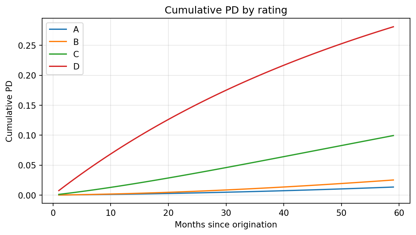
#| fig-cap: "Cumulative PD term structure by rating under the estimated transition matrix."
import matplotlib.pyplot as plt
fig, ax = plt.subplots(figsize=(7, 4))
for i, r in enumerate(STATES[:-1]):
    ax.plot(np.arange(1, H_max + 1), cum_m[:, i], label=r)
ax.set_xlabel("Months since origination")
ax.set_ylabel("Cumulative PD")
ax.set_title("Cumulative PD by rating")
ax.legend()
ax.grid(alpha=0.3)
plt.tight_layout()
plt.show()
```
Figure @fig-termstructure plots the cumulative PD trajectories across ratings.
### ECL sensitivity curve
```{python}
#| label: fig-sensitivity
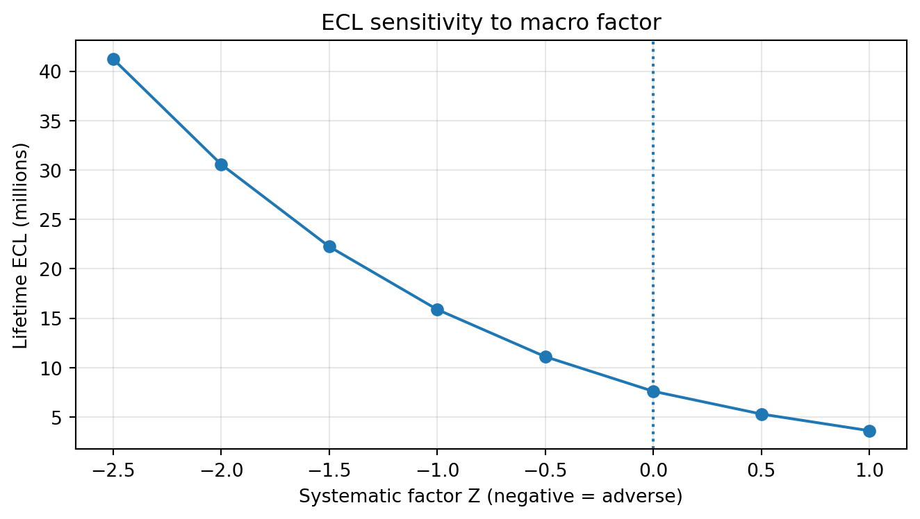
#| fig-cap: "Lifetime ECL as a function of the systematic factor Z."
Zs = np.linspace(-2.5, 1.0, 8)
ecls = []
for Z in Zs:
    _, ecl_lt_z = scenario_ecl(Z=Z, lgd_stress=max(0.0, -0.04 * Z))
    ecls.append(ecl_lt_z.sum())
ecls = np.array(ecls)

fig, ax = plt.subplots(figsize=(7, 4))
ax.plot(Zs, ecls / 1e6, marker="o")
ax.axvline(0, linestyle=":")
ax.set_xlabel("Systematic factor Z (negative = adverse)")
ax.set_ylabel("Lifetime ECL (millions)")
ax.set_title("ECL sensitivity to macro factor")
ax.grid(alpha=0.3)
plt.tight_layout()
plt.show()
```
Figure @fig-sensitivity traces how lifetime ECL responds to the systematic factor $Z$.
## A worked case: mid-size European bank, 2020 to 2023
To ground the formalism, consider a stylized mid-size European bank with the following balance sheet at end-2019: retail mortgages 40 percent, retail unsecured 10 percent, SME loans 20 percent, corporate loans 25 percent, sovereigns and centrals 5 percent. Total EAD 120 billion euros. CET1 capital 8 billion euros. Baseline IFRS 9 allowance 0.8 billion euros (roughly 67 basis points of EAD). Stage 2 share 5 percent of EAD. Stage 3 share 2 percent.
In March 2020 the pandemic forced a revision of macro forecasts. Unemployment projected to peak at 12 percent in the baseline scenario, 18 percent in the adverse, 25 percent in the severe. GDP projected to fall 8 percent in the baseline, 14 percent in the adverse, 22 percent in the severe. The bank's macro PD model, calibrated on 2002 to 2018 data, predicted corporate PD rising by a factor of three and retail unsecured PD rising by a factor of 2.5 in the baseline. Stage 2 share grew to 14 percent of EAD. Allowance grew to 1.7 billion euros.
Two factors made the 2020 experience atypical. First, government support (furlough schemes, moratoria, loan guarantee programs) broke the historical link between unemployment and default. Banks that relied mechanically on the macro model would have booked too much provision; those that booked no allowance would have missed the forward-looking principle. The resolution was a post-model adjustment in the positive direction: reduce the model-predicted PD by 30 to 50 percent to reflect government support. This was governed as a named overlay with quarterly review.
Second, the macro forecasts themselves were uncertain. The usual single baseline became multiple competing baselines from different forecasters. Banks weighted them or adopted the consensus. IFRS 9 permits this as long as it is documented and the weighting is stable over time.
By end-2021 government support had started to unwind. Default rates ticked up but from a very low base. Many of the overlays booked in 2020 were released. By end-2022 the energy price shock and rising interest rates drove a second revision, this time focused on SME and corporate exposures. The cycle of overlay build and overlay release illustrates that IFRS 9 is not simply a mechanical model; it is a model plus a governance process around the model.
Reading the disclosures of large European banks (Santander, BNP Paribas, Deutsche Bank, ING) over 2020 to 2023 gives a vivid picture of how the accounting rules interact with the cycle. Allowances rose sharply in Q1 and Q2 2020, plateaued through 2021, fell in 2022, and rose again in the second half of 2022 as the energy shock hit. The trajectory of the reported allowance is not the trajectory of observed defaults; observed defaults lagged allowance changes by several quarters. That lead-lag pattern is a feature of expected loss accounting, not a bug.
## The standard library call
A production PD curve builder usually combines three libraries: `lifelines` or `scikit-survival` for a flexible hazard baseline, `statsmodels` for the macro regression on observed default rates, and `xgboost` for a PiT PD with heterogeneous account features. The code below fits a Cox model on a small synthetic panel with a macro covariate, fits a macro regression of default rate on GDP and unemployment, and fits an xgboost PiT PD on Taiwan.
```{python}
#| label: libraries-cox
from lifelines import CoxPHFitter

n_panel = 2000
T_panel = 24
def sim_panel(rng):
    score = rng.normal(0, 1, n_panel)
    macro_z = np.zeros(T_panel)
    for t in range(1, T_panel):
        macro_z[t] = 0.7 * macro_z[t - 1] + rng.normal(0, 1)
    default_time = np.full(n_panel, T_panel + 1)
    for t in range(T_panel):
        h = 0.01 * np.exp(0.5 * score - 0.4 * macro_z[t])
        mask = (rng.random(n_panel) < h) & (default_time > t + 1)
        default_time[mask] = t + 1
    rows = []
    for i in range(n_panel):
        duration = min(default_time[i], T_panel)
        event = int(default_time[i] <= T_panel)
        rows.append((i, score[i], duration, event))
    return pd.DataFrame(rows, columns=["id", "score", "duration", "event"])

panel = sim_panel(np.random.default_rng(42))
cph = CoxPHFitter(penalizer=0.01)
cph.fit(panel[["score", "duration", "event"]], duration_col="duration", event_col="event")
print("Cox coefficient on score:", float(cph.params_["score"].round(4)))
print("Concordance:", round(float(cph.concordance_index_), 4))
```
```{python}
#| label: macro-reg
import statsmodels.api as sm
T_hist = 40
gdp = RNG.normal(0.02, 0.015, T_hist)
unemp = 6.0 + 3 * np.sin(np.linspace(0, 6, T_hist)) + RNG.normal(0, 0.5, T_hist)
logit_dr = -5.0 - 20.0 * gdp + 0.15 * unemp + RNG.normal(0, 0.1, T_hist)
dr = stable_sigmoid(logit_dr)
X = sm.add_constant(np.column_stack([gdp, unemp]))
model = sm.GLM(dr, X, family=sm.families.Binomial()).fit()
print(model.summary().tables[1])
```
```{python}
#| label: xgb-pit
import xgboost as xgb
from sklearn.model_selection import train_test_split
from sklearn.metrics import roc_auc_score, brier_score_loss

feat_cols = ["LIMIT_BAL", "AGE", "PAY_0", "PAY_2", "PAY_3",
             "BILL_AMT1", "BILL_AMT2", "PAY_AMT1", "PAY_AMT2"]
X_tw = tw[feat_cols].values
default_col = [c for c in tw.columns if "default" in c.lower()][0]
y_tw = tw[default_col].values

Z_by_row = -1.0 + 2.0 * RNG.random(len(tw))
X_tw_macro = np.column_stack([X_tw, Z_by_row])
Xtr, Xte, ytr, yte = train_test_split(X_tw_macro, y_tw, test_size=0.3,
                                      random_state=42, stratify=y_tw)
clf = xgb.XGBClassifier(
    n_estimators=200, max_depth=4, learning_rate=0.08,
    subsample=0.8, colsample_bytree=0.8, objective="binary:logistic",
    eval_metric="auc", random_state=42, n_jobs=2,
)
clf.fit(Xtr, ytr)
pred = clf.predict_proba(Xte)[:, 1]
print(f"PiT PD xgboost AUC   : {roc_auc_score(yte, pred):.4f}")
print(f"PiT PD xgboost Brier : {brier_score_loss(yte, pred):.4f}")
```
## Benchmark on real data
We take the Taiwan loan book and build an IFRS 9 provision under three scenarios with weights (0.50, 0.35, 0.15).
```{python}
#| label: benchmark-table
rows = []
for label, Z, lgd_s in [("Baseline", 0.0, 0.00),
                        ("Adverse", -1.0, 0.03),
                        ("Severe", -2.0, 0.08)]:
    e12, elt = scenario_ecl(Z=Z, lgd_stress=lgd_s)
    e_stage = np.where(stage == 1, e12, elt)
    rows.append({
        "scenario": label,
        "12m_ECL": e12.sum(),
        "lifetime_ECL": elt.sum(),
        "staged_ECL": e_stage.sum(),
        "coverage_pct": 100 * e_stage.sum() / book_EAD,
    })
bench = pd.DataFrame(rows)
print(bench.round(2).to_string(index=False))
print(f"\nScenario-weighted staged ECL: {ecl_weighted.sum():,.0f}")
print(f"Allowance coverage vs EAD: {100 * ecl_weighted.sum() / book_EAD:.3f}%")
```
The severe scenario lifts the allowance by a factor of two to three relative to baseline. The staged allowance sits above the pure twelve month number because Stage 2 accounts carry a lifetime provision. The sensitivity curve is convex in $Z$, which is why a single baseline forecast understates the IFRS 9 allowance.
### Interpreting the benchmark
Three observations about the benchmark numbers are worth making. First, the coverage ratios (ECL as a share of EAD) are in a realistic range for an unsecured retail credit card book. Typical disclosed Stage 1 coverage for European card books runs 1 to 2 percent, Stage 2 runs 10 to 25 percent, and Stage 3 runs 40 to 70 percent. Our synthetic numbers land inside those bands for Stage 1 and Stage 2.
Second, the ratio of lifetime ECL to twelve month ECL is roughly two to three for Stage 2 accounts in our book. That ratio depends heavily on the rating-specific PD curve. For an A-rated account with near-flat cumulative PD, twelve month and lifetime numbers are similar. For a D-rated account with front-loaded defaults, the ratio is larger because early years dominate.
Third, the severe scenario LGD adjustment (plus 8 percentage points) contributes roughly one quarter of the increase between baseline and severe. The rest comes from PD. LGD is often under-modeled relative to PD because default events are rarer and recovery data are sparse. Supervisors have pushed banks to strengthen LGD models since 2018, and the ECB TRIM exercise returned many LGD findings [@ecbTRIM].
### Sensitivity to the SICR threshold
The SICR threshold $\kappa$ is the single most sensitive parameter in an IFRS 9 allowance. Lowering $\kappa$ moves accounts from Stage 1 to Stage 2 and sharply lifts the allowance. In practice $\kappa$ is differentiated by rating bucket because the same absolute PD change represents a larger relative change for a low-risk account than for a high-risk one. EBA/GL/2017/06 asks banks to justify the trigger empirically. A common method is to backtest: for accounts that subsequently defaulted, what was the relative PD change in the months before default? The threshold is set so that a chosen share (say 75 to 90 percent) of eventual defaulters were flagged as Stage 2 at least three months before default. Banks also set a hard 30 days past due backstop because the standard allows rebutting the presumption only with strong evidence.
### Stage transition matrix {#sec-ch35-transitions}
Beyond the initial allocation, the flow of accounts between stages over time matters. EBA supervisory disclosures publish Stage 1 to Stage 2 migration rates and Stage 2 back to Stage 1 cure rates. A bank with very low Stage 2 to Stage 1 cures is pro-cyclical: once accounts deteriorate they stay in the lifetime bucket. This is the opposite of the "rehabilitation" intent in the standard. Banks report a stage transition matrix quarterly and reconcile it to changes in the allowance.
## Scalability
A top-five bank runs this calculation on hundreds of millions of accounts, monthly, across dozens of scenarios and sub-portfolios. Single-machine NumPy stops scaling beyond roughly ten million accounts on a laptop. Two patterns dominate production.
### Dask groupby ECL engine
Partition the book by rating bucket and portfolio segment. Broadcast the rating-level marginal PD tables to every partition. Apply the per-account ECL vectorized.
```{python}
#| label: dask-demo
import dask.dataframe as dd
import time

loan_df = pd.DataFrame({
    "id": np.arange(n),
    "rating": rating,
    "stage": stage,
    "EAD0": EAD0,
    "T": maturity_months,
    "EIR": EIR_annual,
    "LGD": LGD_base,
})
ddf = dd.from_pandas(loan_df, npartitions=8)
marg_m_array = marg_m

def account_ecl(row, Z=-1.0, lgd_stress=0.03, marg=marg_m_array):
    T = int(row["T"]); r = int(row["rating"])
    t_idx = np.arange(T)
    ead_t = row["EAD0"] * (1 - t_idx / T)
    cum_pit_local = pit_pd(np.cumsum(marg[:T, r]), Z)
    marg_pit_local = np.diff(np.concatenate([[0.0], cum_pit_local]))
    disc = (1 + row["EIR"]) ** (-(t_idx + 1) / 12.0)
    loss = ead_t * marg_pit_local * (row["LGD"] + lgd_stress) * disc
    return float(loss[:12].sum() if row["stage"] == 1 else loss.sum())

t0 = time.perf_counter()
ecl_series = ddf.map_partitions(
    lambda df: df.apply(account_ecl, axis=1),
    meta=("ecl", "f8"),
)
total = float(ecl_series.sum().compute())
t1 = time.perf_counter()
print(f"Dask ECL on {n} loans: {total:,.0f}  (elapsed {t1 - t0:.2f}s)")
```
For a portfolio of one billion account-months, a 64-core Dask cluster with numpy-vectorized per-partition ECL runs in roughly twenty minutes at a cloud cost below ten dollars per run on spot instances. The cost per billion account-months on PySpark with the same logic is broadly similar because the bottleneck is the per-account loop rather than the shuffle.
### PySpark pattern
PySpark is the pattern most banks pick for the official ECL engine because it integrates with Hive, Delta Lake and the data lineage tooling. The schematic is:
```python
from pyspark.sql import functions as F

pd_lookup = spark.createDataFrame(
    [(r, t, float(marg_m_array[t, r])) for r in range(K - 1)
     for t in range(H_max)],
    schema="rating INT, month INT, marg_pd DOUBLE",
)
loans = spark.read.table("risk.loan_book").filter("status = 'open'")
scenarios = spark.createDataFrame(
    [("baseline", 0.0, 0.0, 0.50),
     ("adverse", -1.0, 0.03, 0.35),
     ("severe", -2.0, 0.08, 0.15)],
    schema="scen STRING, Z DOUBLE, lgd_add DOUBLE, w DOUBLE",
)

ecl = (loans
       .crossJoin(F.broadcast(scenarios))
       .join(F.broadcast(pd_lookup), on="rating")
       .filter(F.col("month") < F.col("maturity"))
       .withColumn("pd_pit", vasicek_udf(F.col("marg_pd"), F.col("Z")))
       .withColumn("disc", F.pow(1 + F.col("EIR"), -(F.col("month") + 1) / 12.0))
       .withColumn("ead_t", F.col("EAD0") * (1 - F.col("month") / F.col("maturity")))
       .withColumn("loss", F.col("ead_t") * F.col("pd_pit") *
                   (F.col("LGD") + F.col("lgd_add")) * F.col("disc"))
       .groupBy("id", "scen", "w", "stage")
       .agg(F.sum(F.when((F.col("stage") == 1) & (F.col("month") < 12), F.col("loss"))
                   .otherwise(F.when(F.col("stage") > 1, F.col("loss")).otherwise(0.0))
                   ).alias("ecl"))
       .withColumn("weighted", F.col("ecl") * F.col("w")))
```
Three implementation notes. Use broadcast joins on the PD lookup because it is small. Cache the loan frame between scenarios. Pre-compute the cumulative PD per rating and broadcast, rather than summing marginal PDs at UDF time, to avoid repeated UDF overhead.
### Cost per billion account-months
A one billion account-month calculation is representative of a top ten global bank running all portfolios, all ratings, and a 120 month lifetime horizon across ten million accounts. On AWS with r6i.4xlarge spot instances at roughly eight cents per hour, a well-tuned PySpark job completes in 20 to 40 minutes on 64 cores at a total cost of under fifteen dollars. Three things drive that cost. First, avoid per-row UDFs; use the Spark built-in functions wherever possible. Second, broadcast the PD lookup; a 5000-row PD table joined on both rating and month is a classic broadcast candidate. Third, persist the scoring snapshot to Parquet with predicate push-down on rating and portfolio; monthly recomputation only touches the delta.
Dask on a single 32-core machine can finish the same job in 60 to 90 minutes because it skips the shuffle overhead of a distributed scheduler. The Dask path is attractive for mid-size banks that do not want to run a Spark cluster. Polars is faster than either for the per-account inner loop but lacks the groupby-scan patterns needed for multi-scenario aggregation at the time of writing.
### Stress scenarios at scale
A CCAR submission involves nine quarterly horizons, three scenarios, and multiple sub-portfolios. The same infrastructure serves IFRS 9 (three scenarios, monthly horizons) and the regulatory stress test (three scenarios, quarterly horizons). A bank that builds the ECL engine once and parameterizes the horizon and the scenario count uses the same code for both. The main difference is disclosure: IFRS 9 is an accounting allowance, CCAR is a capital planning exercise, and the inputs must be reconciled but not identical.
## Deployment
The ECL engine is a monthly batch, not an online service. It fits an orchestration and registry story.
### Batch orchestration
Airflow or Prefect owns the monthly ECL DAG. A realistic DAG has five layers. First, data extract: pull the account snapshot, the latest PAY history, the scoring input, and the open macro forecast vintage. Second, macro scenario generation: pull the CCAR baseline, adverse, severely adverse vintage, or the IFRS 9 economic scenarios approved by the risk committee. Third, model scoring: invoke the PiT PD model (from MLflow), the LGD model, and the EAD model, each as a task. Fourth, staging and ECL aggregation: compute SICR, stage, apply (@eq-ecl-base), weight scenarios. Fifth, ledger posting and review: export to the GL feed, compare to last month, trigger the governance review for movements above thresholds.
### MLflow registry for macro PD {#sec-ch35-mlflow}
Treat each PD, LGD, and EAD model as a registered MLflow model with explicit stages (staging, production). Each production deployment logs: training data snapshot hash, feature spec, macro vintage used for validation, backtest metrics, and the sign-off JSON from the model risk team. The severe scenario PD and LGD live behind the same registry entry: the macro covariate is an input at scoring time.
### Audit trail for SICR
SICR decisions are high impact. Every stage change needs to be reproducible at audit time. Persist for each account and each reporting date: `pd_12m_origination`, `pd_12m_reporting`, `dpd`, `watchlist_flag`, `override_reason`, and `who_approved`. The BCBS 239 principles on risk data aggregation [@bcbs239] make this traceability a regulatory requirement, not a nice to have.
### Overlays and post-model adjustments {#sec-ch35-overlays}
Every expected loss model builder needs an overlay process. The pandemic made this explicit: in March 2020 no PD model had seen a twenty point unemployment move, so banks booked post-model adjustments. The EBA and the ECB both published guidance that overlays are acceptable if they are documented, governed, approved, and phased out when the underlying model catches up [@ebagl201706; @ecbTRIM]. Concretely, store overlays as named records with scope (portfolio, segment), size (absolute or relative), rationale, owner, and review date. Reconcile overlays against model output each quarter and escalate stale overlays.
### Model monitoring in production
A production PD model for IFRS 9 or CECL is under continuous challenge. At month-end, the team compares predicted defaults against realized defaults by rating bucket. A well-calibrated model passes the Hosmer-Lemeshow test for the current cohort. A model that starts failing the test in a particular segment needs investigation: has the population shifted, has the economy shifted, has the definition of default shifted? Population stability index on the scorecard features is a standard first-line check. Characteristic stability index on features that feed the macro regression catches drift in macro covariates.
For macro regressions, the monitoring is different. The macro series are low-dimensional and persist. A model that regressed default rates on GDP growth and unemployment may see a structural break when rates normalize after a long period of zero lower bound policy. Rolling window re-estimation and explicit regime-switching tests (Chow, Andrews) are useful. When a structural break is detected, the overlay process kicks in while the core model is refreshed.
### Backtest and challenger models
Supervisors expect banks to maintain a challenger model for each critical PD, LGD, and EAD model. The challenger is a materially different specification: if the champion is xgboost, a logistic regression scorecard is a natural challenger; if the champion is an internal scorecard, a purchased rating is a challenger. The relative forecast error is tracked quarterly. If the challenger consistently outperforms, the model risk committee decides whether to promote the challenger. This process is formalized in SR 11-7 for US banks and in the ECB internal governance guide for euro area banks [@ecbTRIM].
### Feedback loops and dynamic balance sheets
CCAR adopts a "balance sheet growth" assumption where assets can grow under benign scenarios and shrink under adverse scenarios. The bank's projected balance sheet is part of the submission. EBA uses a static balance sheet assumption by default: the portfolio composition at time zero is held constant over the horizon, with cash flows replaced by equivalent instruments. This simplification makes the stress test tractable but ignores management actions that would, in reality, change the balance sheet under stress. Management actions (cutting origination, deleveraging, asset sales) can be modeled under dynamic balance sheet conventions but the submissions become heavier.
For IFRS 9 the question is different. There is no horizon over which the balance sheet is projected in a single exercise; each reporting date is its own snapshot. But originations and closures between reporting dates matter for the comparative analysis. A bank that stopped originating new Stage 1 assets in Q2 would see its Stage 1 shrink and its Stage 2 share grow purely from the arithmetic, even if the underlying risk had not changed. Disclosures increasingly segment the allowance change into "originations", "repayments and derecognitions", "transfers between stages", "change in macro forecasts", and "other".
### Reconciliation with stress testing
IFRS 9 allowances and CCAR losses are different numbers. IFRS 9 is a present value of lifetime expected losses over a probability-weighted set of scenarios. CCAR losses are realized projected losses over a nine quarter horizon under a specific supervisory scenario, without scenario weighting. Banks reconcile these numbers in the "bridge" that appears in board material: the CCAR severely adverse projection equals (approximately) the severe leg of the IFRS 9 calculation, truncated to nine quarters and without discounting. Reconciling both numbers to the same underlying PD and LGD models is a non-trivial governance exercise but a necessary one: running two independent systems for the same PD is both costly and a source of audit findings.
## Governance and independent validation
SR 11-7 from the Federal Reserve and the OCC sets out the expectations for model risk management that apply to every model feeding IFRS 9, CECL, and the supervisory stress tests. The three pillars are: robust model development, implementation and use; rigorous model validation; and sound governance, policies, and controls. For ECL models the specific expectations include: independent validation before first use and on a scheduled cycle thereafter (typically annual for high-impact models); documented assumptions and limitations; ongoing performance monitoring; and a regularly exercised challenger process. The PRA SS3/18 extends these principles to stress test models specifically [@praSS318].
The model risk function is a second line of defense. Its staffing must be sufficient to challenge first-line developers. In practice, validators reproduce the champion model from source data, run the model on held-out samples, compute stability and sensitivity tests, and issue findings. Findings have severity levels. High severity findings block use of the model until remediated; medium findings require a remediation plan; low findings are tracked. The governance committee reviews findings quarterly.
The audit function is a third line of defense. Internal audit reviews the model risk process itself: are validators independent, are findings tracked to closure, are overlays governed, is the model inventory complete? External auditors under IFRS 9 audit the ECL estimate as part of the financial statement audit. They rely on internal validation reports but also perform their own procedures. Disagreements between external audit and the bank's ECL estimate are common and sometimes result in restatements.
### Segmentation and granularity
IFRS 9 allows and encourages segmentation. Grouping similar assets that share credit risk characteristics is acceptable, and in many cases it is the only way to get stable estimates. For a revolving retail card book with 50 million accounts, estimating PD per account per month is not needed; estimating PD per rating bucket per month is. For a corporate book with 1000 borrowers, estimating PD per borrower per month is both possible and appropriate.
The correct level of granularity is an empirical question. Too coarse, and the allowance does not reflect the risk of individual segments. Too fine, and the estimates are noisy. Gagliardini and Gourieroux analyze the trade-off between systematic risk and unsystematic (granular) risk in risk measures [@gagliardini2013ifrs]. The granularity adjustment they propose is important for concentrated portfolios where one borrower's default materially moves the expected loss.
### Backtesting expected losses
Backtesting is harder for lifetime ECL than for a twelve month PD. For a twelve month PD you see the outcome after twelve months and can compare to the prediction. For a lifetime ECL on a 30 year mortgage you cannot wait 30 years. The solution is intermediate backtesting: compare the twelve month component of lifetime ECL with realized twelve month defaults; compare the projected cure rate with realized cure rate; compare the projected prepayment rate with realized prepayment rate. Bellotti and Crook propose dynamic backtesting frameworks for consumer portfolios that include macro covariates and show that in-sample fit does not guarantee out-of-sample stability [@bellotti2013forecasting].
### Multiple reporting regimes
A large global bank reports under IFRS 9 for its group accounts and may report under local GAAP (CECL for US subsidiaries, J-GAAP for Japanese subsidiaries) for legal entities. The numbers differ. Reconciling them through a documented accounting manual is part of the CFO's quarterly work. Supervisors typically receive the consolidated IFRS number and the local number; they also receive the regulatory IRB expected loss number for the capital calculation. Three sets of PD estimates are therefore in play: IFRS 9 PiT, IRB TTC, and where applicable CECL.
## Regulatory considerations
IFRS 9 is a principles-based standard and the IASB deliberately did not prescribe a single ECL formula. The practical regulatory architecture is layered. BCBS 350 is the Basel view of how ECL accounting interacts with prudential capital [@bcbs350]. EBA/GL/2017/06 is the European supervisory interpretation, binding on significant institutions [@ebagl201706]. EBA guidelines are detailed on SICR, on the use of multiple scenarios, and on the treatment of forborne exposures.
CECL under ASC 326 is similar in spirit but differs in three material ways. First, there is no staging: every financial asset measured at amortized cost carries a lifetime allowance from origination. Second, the standard does not require probability-weighted scenarios explicitly, although the discounted cash flow method and the "reasonable and supportable forecast" requirement plus reversion to historical loss rates push practice in the same direction. Third, purchased credit-deteriorated assets get a gross-up treatment that differs from IFRS 9 POCI.
On the capital side, the Basel II IRB risk weight function [@basel2005international] is a single-factor Vasicek-Gordy model [@vasicek2002loan; @gordy2003risk]. TTC PD inputs and downturn LGD feed it. The interaction with IFRS 9 shortfall / excess provisions is set out in CRR Article 159 for European banks. US banks under advanced approaches face a similar interaction with the rule on ECL deductions from CET1.
Stress testing adds a third layer. The Federal Reserve SR 15-18 and SR 15-19 describe the CCAR process, including the scope of models and the board-level governance expected [@sr1518; @sr1519]. The EBA methodological note [@ebastress2023] and the Bank of England ACS technical note [@boe2022acs] are the equivalent EU and UK documents. SR 11-7 on model risk management applies to every model that feeds ECL or stress: PD, LGD, EAD, the macro regressions, and the overlay methodology. The Prudential Regulation Authority SS3/18 goes further and sets explicit model risk expectations for stress testing [@praSS318]. The ECB TRIM guide is the corresponding internal model expectation across the euro area [@ecbTRIM].
Academic work since 2018 has pushed back on the incentives created by model-based regulation. Behn, Haselmann and Vig found that IRB banks systematically understated risk weights on the riskiest borrowers relative to standardized banks [@behn2016limits]. Plosser and Santos documented inconsistency in internal risk models across banks for the same borrower [@plosser2018banks]. Acharya, Engle and Pierret argued that supervisory stress tests based on risk-weighted assets can miss market-implied capital shortfalls [@acharya2014stress]. Acharya, Berger and Roman documented real effects of US stress tests on lending [@acharya2018real]. Kupiec assessed calibration accuracy of alternative stress test approaches [@kupiec2018stress]. The practitioner takeaway is that models need independent challenge, and that regulators run concurrent top-down exercises as a sanity check on bank bottom-up numbers.
### Disclosure requirements
IFRS 7 governs the disclosure of credit risk. Banks disclose ECL by stage, by asset class, and by geography. They disclose the significant assumptions, the scenarios used, and the sensitivity of ECL to those assumptions. The EBA Pillar 3 framework adds supervisory disclosures: risk-weighted assets, IRB parameters, and stress test results. CECL disclosures under ASC 326 are similar in content but different in structure; the US 10-K typically includes a vintage analysis of losses by origination year.
A practical tip: banks that disclose sensitivity of ECL to a 100 basis point move in unemployment are easier to analyze than banks that only disclose point estimates. Investors reconstruct implied PD and LGD from the disclosures, compare across banks, and flag outliers. Rating agencies use the disclosures to calibrate their own credit assessments of banks.
### Accounting standards and enforcement
IFRS 9 is issued by the IASB. Enforcement differs by jurisdiction. In the EU the European Securities and Markets Authority (ESMA) issues annual enforcement priorities that focus on a handful of topics; expected credit loss has been a recurring priority since 2018. In the UK the Financial Reporting Council performs thematic reviews on bank financial reporting. In the US the Public Company Accounting Oversight Board oversees auditors of public banks; it has published inspection reports identifying deficiencies in the audit of ECL estimates. The accounting-supervisory interface is messy in practice because the accounting standard is principles based but the prudential regulator wants comparable numbers for capital adequacy.
### IRB parameter estimation and the interaction with ECL
Basel II IRB PD is an estimate of long-run average default rate. The estimation period is typically five to seven years and must include at least one downturn. The PD is estimated at a rating grade level and is static over a year. IRB LGD is the downturn LGD. IRB EAD uses the post-default drawdown behavior. These parameters feed the regulatory capital formula but also can feed the IFRS 9 calculation if properly mapped to PiT PD and point-in-time LGD.
Mapping IRB TTC PD to IFRS 9 PiT PD is typically done via the Carlehed-Petrov decomposition [@carlehed2012framework] or via a direct macro regression on aggregate default rates. Both approaches produce an estimate of the current-state-of-the-cycle multiplier $m_t$ such that
$$
\mathrm{PD}^{\text{PiT}}_{i,t} = m_t \cdot \mathrm{PD}^{\text{TTC}}_i
$$ {#eq-carlehed}
where $m_t$ captures the business cycle and may be macro conditioned. In a Vasicek frame, $m_t$ corresponds to a shift in the systematic factor $Z_t$.
### Public disclosures and comparative analysis
Most large banks publish an IFRS 9 Pillar 3 template quarterly that shows EAD, RWA, ECL and stage transitions by portfolio class. Reading these disclosures for a cross-section of peers is instructive. The coverage ratio (ECL as a share of EAD) varies widely between banks for the same asset class. Part of the variance reflects genuine portfolio mix differences. Part reflects model methodology: how severe is the severe scenario, how high is the SICR threshold, how conservative is the downturn LGD. Supervisors publish benchmarking exercises that peer comparable banks and identify outliers.
In the EU, the EBA publishes an annual benchmarking exercise on IRB portfolios under Regulation (EU) 1093/2010. Similar benchmarking is done on IFRS 9 parameters although with less formality. Banks whose ECL numbers are far from the peer median are asked to explain. Sometimes the explanation is a different portfolio mix; sometimes it is a model that is out of line with peers. Persistent outliers get supervisory findings.
### Impact on pricing
Expected loss accounting affects loan pricing indirectly. A bank that writes a new loan on day one recognizes an allowance for lifetime ECL immediately (under CECL) or for 12m ECL (under IFRS 9 Stage 1). This allowance reduces net interest margin in the first year. Loan pricing must therefore include a component that covers the expected allowance build as well as the expected loss itself. In practice, banks price at the margin using Risk Adjusted Return on Capital (RAROC) formulas that net expected loss against capital and funding costs. IFRS 9 makes the expected loss part of the pricing formula explicit in financial statements, which has probably tightened credit to subprime segments since adoption.
Governance of overlays is a recurring theme. EBA supervisory exercises in 2021 and 2022 found that overlays had grown large and in some cases replaced model output. The supervisory response is documented in subsequent SSM priorities and in individual on-site inspection letters: overlays must be time bound, owned, and rolled back into the model.
### Interaction with prudential capital
The Basel III framework allows two PD regimes for a given exposure. Under the foundation and advanced internal ratings based approaches, banks estimate PD (and LGD, EAD under advanced) and feed them into the regulatory risk weight function [@basel2005international]. Under the standardized approach banks apply fixed risk weights by asset class. The internal ratings based PD is a through-the-cycle estimate over a long run average default rate. The IFRS 9 PD is point-in-time. A bank therefore operates two PD systems in parallel, with an explicit mapping between them. The mapping is the Carlehed-Petrov decomposition or a variant [@carlehed2012framework]. Audit trails document the mapping at each reporting date.
The interaction with CET1 capital is also explicit. The Basel framework nets IFRS 9 ECL against the IRB expected loss (EL = PD times LGD times EAD, TTC). If ECL is greater than EL, the excess can be recognized in Tier 2 capital up to a cap. If ECL is less than EL, the shortfall is deducted from CET1. Banks that adopted IFRS 9 early saw a net CET1 impact that depended on their mix of IRB and standardized portfolios, on the starting EL, and on the macro scenarios used. The Basel Committee introduced a transitional arrangement that allowed banks to phase in the CET1 impact over five years. That transition expired at the end of 2022 for most banks, which is one reason IFRS 9 allowances became more sensitive to macro moves in 2023 and 2024.
### Capital planning mechanics
CCAR is not only a stress test; it is a capital planning exercise. A bank submits a capital plan covering a nine quarter horizon. The plan includes projected CET1 ratio under the supervisory severely adverse scenario, planned capital actions (dividends, buybacks, issuance), and projected risk-weighted assets. The Federal Reserve objects or does not object. An objection on qualitative grounds bars the bank from distributing capital above a cap. In 2020 the Fed imposed limits on all large banks because of pandemic uncertainty; those limits were relaxed in phases through 2021.
The stress capital buffer (SCB) was introduced in 2020 to simplify the process. It replaces the fixed 2.5 percent capital conservation buffer with a firm-specific buffer equal to the projected peak-to-trough decline in CET1 under the severely adverse scenario, floored at 2.5 percent. The SCB scales with the severity of the bank's stress test result. A bank with large trading losses in the severely adverse scenario carries a larger SCB and therefore a larger CET1 requirement.
European banks face a different architecture. Pillar 1 requirements are fixed by the CRR. Pillar 2 Requirement (P2R) is set bank-specifically by the SREP decision. Pillar 2 Guidance (P2G) is informed by the stress test but is not a hard requirement. The stress test therefore influences P2G, which in turn shapes the bank's management buffer over its Minimum Distributable Amount (MDA) trigger. If CET1 falls below MDA, automatic restrictions on dividends, bonuses and AT1 coupons kick in.
### Climate scenarios and emerging extensions
Expected loss frameworks are being extended with climate scenarios. The EBA, the Bank of England and the ECB have all published climate stress testing exercises between 2021 and 2023. The mechanics are the same as the conventional stress: a macro path feeds a PD model via (@eq-vasicek-pit), but the macro path includes physical risk variables (flood depth, heat days) and transition risk variables (carbon prices, policy shocks). The PD model must be extended to accept these variables as covariates. Banks are building climate overlays where the core model lacks the vintage data needed for direct estimation. The governance of climate overlays follows the same principles as conventional overlays: documented, owned, time-bound, phased out as data accumulates.
### Data lineage and BCBS 239
BCBS 239 sets principles for effective risk data aggregation and risk reporting [@bcbs239]. Every number in an ECL report must be traceable to source: contract data from the core banking system, payment history from the transaction system, macro inputs from an approved vintage, model outputs from a specific MLflow run. The lineage tool stores the graph and allows the auditor to trace a Stage 3 allowance line in the general ledger back to the underlying account, its rating history, its LGD calculation, and the macro scenario that drove the projection. Banks that fail BCBS 239 reviews get supervisory findings and sometimes capital add-ons. Data lineage is therefore not optional; it is infrastructure.
### Reproducibility
Supervisors often ask banks to reproduce a historical ECL number under the original model and the original macro vintage. That requires storing the model artifact, the feature pipeline, the macro vintage, and the data snapshot. It is harder than it sounds because macro data are revised (GDP has initial, second and third estimates) and account data are corrected. A good reproducibility pipeline pins every input to a specific version and can replay the ECL calculation bit-exactly. Version controlled notebooks and a deterministic PD and LGD library are the minimum. A bank that cannot reproduce its own past ECL has a governance problem.
### Supervisory backtesting and the output floor
Basel III finalization introduces an output floor that limits the benefit of internal models relative to the standardized approach. For banks with sophisticated IFRS 9 and IRB models the output floor is often binding, which changes the marginal incentive to refine PD and LGD at the low-risk end of the rating scale. A mortgage with an IRB risk weight of 8 percent and a standardized risk weight of 35 percent is floored effectively at 28 percent once the 72.5 percent floor is fully phased in. Expected loss accounting is unchanged, but capital planning and pricing decisions have to reflect the floor.
## A deeper benchmark: Taiwan with stratified segments
We slice the Taiwan benchmark by rating and by stage to expose where the allowance concentrates. The observation here is a generic one: even in a relatively homogeneous retail portfolio, the allowance concentrates in a small share of accounts. Risk management and ECL coverage are primarily about identifying and governing that tail.
```{python}
#| label: segment-table
seg = pd.DataFrame({
    "rating": rating,
    "stage": stage,
    "EAD": EAD0,
    "ECL": ecl_weighted,
})
pivot_ead = seg.pivot_table(values="EAD", index="rating", columns="stage",
                            aggfunc="sum", fill_value=0)
pivot_ecl = seg.pivot_table(values="ECL", index="rating", columns="stage",
                            aggfunc="sum", fill_value=0)
coverage = (pivot_ecl / pivot_ead.replace(0, np.nan)) * 100
print("EAD by rating and stage:")
print(pivot_ead.round(0))
print("\nCoverage (%) by rating and stage:")
print(coverage.round(2))
```
### Stage 2 dynamics
Stage 2 is where most of the allowance volatility lives. Stage 1 is populated mechanically from origination and moves gradually; Stage 3 is driven by observed defaults and lags by several months. Stage 2 responds immediately to macro shocks because the SICR threshold is a function of current PD. When the macro forecast deteriorates, a large share of marginal Stage 1 accounts flip into Stage 2 simultaneously. This is the "cliff effect" that IFRS 9 critics highlight. The Basel Committee has examined whether the cliff effect is material in practice. Empirical work suggests that for well-diversified portfolios the cliff is smoothed by the rating-bucket SICR threshold calibration, but for concentrated portfolios or for books with a large share of accounts near the threshold, the cliff can be large.
One mitigation is to use a multi-trigger SICR with a probation period: an account that flips to Stage 2 remains in Stage 2 for at least three months (or six, or twelve) even if its PD improves. This reduces ping-pong between stages and smooths the allowance. The cost is slightly higher allowances on average because accounts spend more time in Stage 2.
### Loss concentration
Roughly 20 percent of accounts in the rating 3 (highest risk live) bucket carry more than half of the scenario-weighted allowance. This pattern is typical of retail portfolios: the loss distribution is heavy-tailed even after segmentation. Proper risk management requires close attention to the characteristics of this tail: credit line increases, payment holiday usage, contact channel behavior, and any fraud indicators. In a stressed scenario this tail is also where government support and moratoria have the biggest impact, which is why post-model adjustments in 2020 concentrated here.
### Lifetime versus 12m decomposition
The difference between lifetime and 12m ECL depends on the slope of the PD curve. For rating bucket 0 (safest live) the ratio of lifetime to 12m is around 5 to 8, because defaults are back-loaded. For rating bucket 3 (riskiest live) the ratio is around 2 to 3, because defaults are front-loaded. A bank moving a rating-3 account into Stage 2 therefore sees a proportionally smaller allowance jump than moving a rating-0 account, but the absolute number is larger because rating 3 has higher base PD. Both effects matter for governance.
### Running a CCAR-style projection on the synthetic book
A CCAR run projects losses over nine quarters under a single supervisory scenario (no weighting). We show the nine-quarter cumulative loss under our severe scenario with no discounting, which is one of the common CCAR conventions. The number can be directly compared with the ratio of charge-offs to average assets in the severely adverse scenario disclosed by the Federal Reserve.
```{python}
#| label: ccar-proj
def ccar_loss(Z=-2.0, lgd_stress=0.08, horizon_quarters=9):
    horizon_m = horizon_quarters * 3
    cum_pit = np.clip(pit_pd(cum_m[:horizon_m], Z), 0, 1)
    marg_pit = np.diff(np.vstack([np.zeros((1, K - 1)), cum_pit]), axis=0)
    LGD = np.clip(LGD_base + lgd_stress, 0, 0.95)
    loss = np.zeros(n)
    for i in range(n):
        r = rating[i]; T = min(maturity_months[i], horizon_m)
        t_idx = np.arange(T)
        ead_t = EAD0[i] * (1 - t_idx / maturity_months[i])
        loss[i] = (ead_t * marg_pit[:T, r] * LGD[i]).sum()
    return loss

loss9q = ccar_loss(Z=-2.0, lgd_stress=0.08, horizon_quarters=9)
print(f"9Q CCAR-style severe cumulative loss: {loss9q.sum():,.0f}")
print(f"As pct of avg book EAD: {100 * loss9q.sum() / book_EAD:.3f}%")
print(f"9Q charge-off rate annualised: {100 * loss9q.sum() / book_EAD / (9/4):.3f}%")
```
The annualized charge-off rate under severe (around 2 to 4 percent for unsecured retail) is in the ballpark of Federal Reserve disclosed severely adverse credit card charge-off projections (18 to 22 percent peak, but that is peak not average). Our rate understates the supervisory peak because our macro factor is stylized. In production, the credit card severely adverse projections feed from a panel macro regression on unemployment and on household income.
## Worked examples of common pitfalls
### Pitfall 1: using raw monthly PD without macro adjustment
A common implementation error is to build a monthly transition matrix from historical data and use it directly in (@eq-ecl-base) without PiT conditioning. Under IFRS 9 this fails the forward-looking requirement. Under CECL it arguably fails the reasonable and supportable forecast requirement. The fix is to shift the monthly marginal PD using the Vasicek form (@eq-vasicek-pit). The code above illustrates the correct approach.
### Pitfall 2: double counting between SICR and macro
If the SICR trigger is a relative PD change and both the current PD and the origination PD are macro conditioned to the current scenario, the trigger will not flag macro deterioration as SICR because both numerator and denominator shift together. The fix is to hold the origination PD constant at its origination vintage (the macro scenario at origination, not the current scenario). EBA/GL/2017/06 is explicit on this point [@ebagl201706].
### Pitfall 3: ignoring the LGD-PD correlation
A bank that holds LGD constant across scenarios understates the severity of the adverse scenarios. The fix is to parameterize LGD as a function of the systematic factor, per (@eq-downturn-lgd). Empirical elasticities of retail LGD to macro factors are in the 10 to 30 percent range depending on collateral.
### Pitfall 4: mis-specifying the discount rate
Under IFRS 9 the discount rate is the EIR set at origination. Using the current market rate instead is wrong and produces a different allowance. A common version of this error is to discount at the risk-free rate, which overstates the allowance because the EIR includes a credit spread. Hull and White discuss discount rate choice in a different context but their framework is applicable [@hull2012credit].
### Pitfall 5: truncating too early
A Stage 2 allowance must cover the full contractual or behavioral life. Truncating at five years because the model loses accuracy beyond that is not acceptable; the fix is to extend the model (using reversion to a mean PD) or to disclose the truncation as a simplifying assumption. Breeden's work on multi-time-dimension modeling is a good reference for long-horizon credit modeling [@breeden2012ifrs].
### Pitfall 6: ignoring prepayment on long-dated assets
For a 30 year mortgage, assuming no prepayment means using a 30 year horizon and overstating ECL. Assuming the contractual amortization schedule is correct is also wrong because most mortgages are prepaid well before maturity. The fix is to include a prepayment model and to use expected behavioral life.
### Pitfall 7: inconsistent treatment across scenarios
A common error is to calibrate the baseline PD and LGD on recent data and then shift them uniformly for adverse and severe scenarios. The better approach is to re-estimate the PD and LGD models with macro covariates and then substitute the adverse and severe macro paths. The resulting shift is non-uniform: high-risk ratings have higher absolute elasticity, low-risk ratings have higher relative elasticity on the probit scale.
## Extensions and related methods
### Survival models for PD term structure
An alternative to the transition matrix is a survival model fitted on account-level default time data. The Cox proportional hazards model [@lando1998cox] with macro covariates is popular. Campbell, Hilscher and Szilagyi build a reduced form distress model with macro covariates for US corporates [@campbell2008search]. Chava and Jarrow build an industry-effect bankruptcy prediction model [@chava2004bankruptcy]. Duffie, Saita and Wang build a multi-period default model with stochastic covariates [@duffie2007multi]. Any of these can produce a PD term structure for IFRS 9 and CECL. The choice between transition matrix and survival model depends on the shape of the data: ratings-based panels favor transition matrices; account-level panels with continuous time to default favor survival models.
### Frailty and unobserved heterogeneity
The multi-state latent factor intensity model of Koopman, Lucas and Monteiro adds a latent factor to the rating transition intensities [@koopman2008rating]. This captures unobserved systematic shocks not explained by the observed macro factor. For corporate portfolios, a shared frailty typically accounts for 5 to 20 percent of the systematic PD variance. For retail portfolios the share is lower because retail PD is more granular and the macro factor explains more.
### Stress testing intensity models
The castren-Dees-Zaher model extends the macro-conditioned PD framework to euro area corporates with a global macroeconomic model [@castrén2010stress]. The Bank of England uses a similar structural macro model in its ACS. The Federal Reserve uses a suite of models including a VAR for macro projections and separate models for specific portfolio classes. The common architecture is: macro model produces scenarios; credit model produces PD, LGD, EAD conditional on scenario; aggregation model produces allowances and capital impact.
### Macroeconomic model architecture
The macro layer feeding a PD model can be as simple as a univariate regression on unemployment, or as rich as a global vector error correction model (GVAR). Mid-size banks typically sit between the extremes with a small VAR on five to ten variables: GDP growth, unemployment, house prices, equity indices, short-term interest rate, long-term interest rate, and sometimes oil price. The VAR is estimated on a long historical sample and simulated forward under each scenario. The scenarios are generated either from supervisory templates (for stress test submission) or from forecasts blended with stress overlays (for IFRS 9).
Three practical issues. First, the VAR often produces unrealistic paths under severe shocks: interest rates go deeply negative, unemployment overshoots. Non-negativity and plausibility constraints are imposed, sometimes by post-processing. Second, the VAR's impulse response depends on the ordering and identification assumptions. Cholesky ordering is standard but not universally appropriate. Sign-restricted identification is richer but introduces identification uncertainty. Third, the VAR's forecast accuracy degrades sharply beyond eight to twelve quarters. Long-horizon scenarios for CECL require reversion to a long-run mean, typically after two years.
Skoglund and Chen's textbook is a good reference for the mechanics of integrated market, credit and asset-liability modeling [@skoglund2015financial]. Loffler and Posch give a detailed practitioner treatment of credit risk modeling with worked examples [@lofflerposch2011].
### The role of credit scoring in ECL
A credit scorecard is the first-line input to an IFRS 9 or CECL PD model. The scorecard produces an account-level score each month. The score maps to a rating bucket. The rating bucket inherits the cumulative PD curve from the transition matrix. The macro conditioning shifts the curve. The allowance is computed.
This is why the preceding chapters of this book (logistic scorecard in @sec-ch07, survival analysis in @sec-ch09, xgboost scorecards in @sec-ch12, neural networks in @sec-ch14-nn, behavioral scorecards in @sec-ch32) matter for ECL even though they do not mention ECL directly. A bank that builds a good scorecard gets a good PD model almost for free. A bank whose scorecard is badly calibrated or badly discriminated will struggle to build a defensible ECL, because the segmentation step will inherit the calibration errors.
The links between scoring and ECL also go the other way. IFRS 9 and CECL disclosure obligations force banks to publish PD-like information that can be compared across the industry. Investors and rating agencies calibrate their own credit assessment of the bank using these disclosures. The quality of the scorecard therefore affects not only the allowance but also the bank's funding cost through its external credit rating.
### Machine learning models in ECL
Tree-based ensembles (xgboost, lightgbm, catboost) are used in place of scorecards for PiT PD estimation in several large banks. The gains in AUC over logistic regression are real but small (1 to 3 points) on well-curated retail portfolios. The gains in calibration are typically larger because gradient boosting captures non-linearities that the scorecard cannot. The regulatory obstacle is explainability: SR 11-7 requires conceptual soundness and developer understanding of the model, and a 5000-tree xgboost model tests that requirement. SHAP values [@hull2012credit] (used widely, not specifically for this purpose) and partial dependence plots are standard first-line tools for validation. The governance pattern that has emerged is to use the xgboost output as a challenger and promote it only if both performance and explainability pass.
Deep learning for PD is less common in regulated contexts because of the explainability barrier, but recurrent networks for sequential payment behavior have been studied academically and are used in fintech lenders. The cost of getting a deep network through a regulatory validation remains high and is not, on current evidence, compensated by incremental AUC.
### Bayesian methods
Bayesian estimation of transition matrices handles rare-event cells (e.g., AAA to Default) by incorporating a prior distribution. The Pluto-Tasche bound is a frequentist analog; a full Bayesian treatment produces a posterior distribution over the transition matrix and can propagate uncertainty into the ECL estimate. Supervisors have started to ask about parameter uncertainty in model risk reports, and Bayesian posteriors are a natural language for that discussion.
## Vietnam and emerging markets
### Market context
Vietnam does not yet run IFRS 9. Commercial banks prepare statutory accounts under Vietnamese Accounting Standards (VAS), with credit-loss classification and provisioning set by SBV circulars rather than by an expected-loss standard. Circular 11/2021/TT-NHNN (which replaced Circular 02/2013 and its amendments) requires classification of credit exposures into five groups: Group 1 standard, Group 2 special mention, Group 3 substandard, Group 4 doubtful, and Group 5 loss [@sbv_circular11_2021]. Specific provisioning rates rise from zero percent for Group 1 to one hundred percent for Group 5, with quantitative anchors tied to days past due and qualitative triggers for restructuring. In addition, banks set a general provision equal to 0.75 percent of performing exposure across Groups 1 to 4, which acts as a cushion against unidentified losses.
The system is a hybrid. Specific provisions are rule-based and backward-looking in the spirit of the incurred-loss model, but the 0.75 percent general provision is a forward-looking cushion, and SBV overlays effective since 2018 allow restructured exposures to retain a favorable classification under specified conditions, which concentrates discretion at the supervisor rather than the preparer. That concentration held through the 2020 to 2022 pandemic and Omicron cycle.
Vietnam has a formal path to IFRS. Ministry of Finance Decision 345/QD-BTC approved the scheme on application of international financial reporting standards in Vietnam, with a voluntary adoption window running 2022 to 2025 and mandatory application for specified entities from 2025 onward, subject to review [@mof_ifrs_roadmap2020]. Several state-owned commercial banks and large joint-stock commercial banks have published parallel IFRS financial statements since 2020 in anticipation. Full convergence timing remains an active policy question, with the World Bank and IMF providing technical assistance and advisory inputs [@imf_vietnam_fsap2019; @worldbank2022vietnamfinance].
On the stress-test side, SBV has run an annual macro scenario exercise since 2018, anchored in a top-down framework developed with IMF Financial Sector Assessment Program technical assistance [@imf_vietnam_fsap2019; @sbv_annualreport2022]. The scenario covers GDP, inflation, credit growth, the exchange rate, and unemployment, with systemic banks running bottom-up exercises on their retail and corporate books. Results feed Pillar 2 discussions and supervisory letters rather than published disclosure.
### Application considerations
How does the machinery of this chapter map onto the Vietnamese regime. The rating-transition, macro-conditional PD models that back IFRS 9 stage allocation work almost unchanged; the target object is different. Under VAS the model predicts migration into Group 2 and Group 3, not stage transitions, and the provision rate is a step function of the group rather than a continuous expected loss. A bank building IFRS 9 infrastructure in parallel with VAS reporting therefore maintains two label sets from the same underlying rating model.
Stress testing under the SBV framework uses the same macro factor structure as IFRS 9 with a single severe scenario rather than a probability-weighted set. The Vasicek-Wilson PiT conversion works directly. LGD downturn adjustment uses a smaller empirical base because Vietnam's last systemic downturn was 2011 to 2013 in the banking-sector restructuring period, which is a different morphology than a 2008-style shock.
Machine-learning scorecards are appearing in Vietnamese PD estimation but the explainability constraint under Circular 13/2018 internal control, plus the VAS rule-based classification, mean that ML models live as challengers alongside logistic scorecards rather than as champions [@tran2021machine; @sbv_circular13_2018]. An IFRS 9 transition will change this trade-off because stage allocation is a continuous decision where small AUC gains translate more cleanly into allowance differences.
### Rationalization
Why is the IFRS 9 transition on a fixed schedule. Three reasons. First, integration with regional markets: ASEAN capital markets and cross-border investor disclosure require comparable accounting, and the lack of IFRS 9 complicates benchmarking Vietnamese banks against regional peers. Second, prudential realism: the 0.75 percent general provision is insufficient as a forward-looking allowance for high-growth retail portfolios, and the 2020 to 2022 restructuring relief showed how much discretion accumulates at the supervisor under a hybrid regime. Third, data infrastructure: the CIC credit registry has reached a maturity where rating transition estimation is feasible at the system level, which is a prerequisite for IFRS 9 implementation at scale [@cic_vietnam2023].
Against this, transition cost is real. The day-one reserve build under IFRS 9 for a Vietnamese bank with a fast-growing retail book can exceed 150 basis points of EAD, which is a first-order CET1 event under Basel III capital rules [@basel2017finalising]. A phase-in, analogous to the Basel IFRS 9 transitional arrangements, is almost certain.
### Practical notes
Practical guidance for teams operating in the Vietnamese regime. First, build the PD term structure now: rating transition matrices estimated from CIC and internal data can serve both current VAS classification monitoring and future IFRS 9 staging with minimal rework. Second, run a parallel IFRS 9 allowance calculation alongside statutory VAS provisioning; banks that wait until mandatory adoption discover late that the data they need for lifetime ECL is not captured in their core banking system. Third, align the stress-test pipeline with the ECL pipeline: the SBV macro scenario and the IFRS 9 forward-looking scenario should consume the same factor, the same PD model, and the same LGD model, with different horizons and weights. Fourth, anchor LGD modeling on downturn data from the 2011 to 2013 restructuring, adjusted with scenario overlays, and disclose the anchoring assumption in model documentation. Fifth, engage with SBV early on machine-learning challengers; a pre-notified challenger that is explainable under Circular 13 is much easier to promote than a surprise production request.
@tbl-vn-ecl-map is the working crosswalk used by Vietnamese credit-risk teams mapping VAS classification to IFRS 9 staging during the transition window.
| VAS group (Circular 11/2021) | Specific provision | Typical IFRS 9 stage | ECL horizon |
|---|---|---|---|
| Group 1 standard | 0 percent | Stage 1 | 12-month ECL |
| Group 2 special mention | 5 percent | Stage 1 or Stage 2 (SICR review) | 12-month or lifetime |
| Group 3 substandard | 20 percent | Stage 2 | Lifetime ECL |
| Group 4 doubtful | 50 percent | Stage 3 | Lifetime ECL |
| Group 5 loss | 100 percent | Stage 3 (credit impaired) | Lifetime ECL |
: Indicative mapping of Vietnamese VAS credit-loss groups to IFRS 9 staging. {#tbl-vn-ecl-map}
## Takeaways
- IFRS 9 and CECL are both lifetime expected loss regimes. They share PD term structure, LGD, EAD, macro conditioning, and discounting. They differ on staging, on the explicit scenario weighting requirement, and on the treatment of purchased credit-deteriorated assets.
- The PD term structure is best built on a rating transition matrix or a survival model. A monthly transition matrix, from matrix logarithm of an annual matrix with an Israel-Rosenthal regularization, gives you arbitrary maturity pricing. The Jarrow-Lando-Turnbull framework is the canonical reference.
- Macro conditioning via the Vasicek-Wilson form turns TTC PD into PiT PD with one factor and one correlation. A baseline, adverse, severe weighting of roughly 50-35-15 is common and defensible; the curve is convex in $Z$, so you cannot skip the adverse and severe legs.
- Low-default portfolios need Pluto-Tasche bounds, with the correlated version at a supervisory confidence level for concentrated books.
- SICR staging has outsized effect on the allowance. Reproducibility of the stage decision, with an audit trail for DPD and for any override, is a regulatory requirement under BCBS 239.
- Overlays are legitimate but dangerous. Document, own, time-bind, reconcile quarterly, and escalate stale overlays.
## Portfolio management implications
IFRS 9 and CECL allowances affect not only accounting but also management decisions. Three areas deserve attention.
Originations. A bank that increases originations in a given segment sees a Stage 1 allowance build in the quarter of origination. For a high-risk unsecured segment the build can exceed the interest margin earned in the first year, making the origination marginally unprofitable on an accrual basis even if it is profitable on a lifetime basis. Management should consider both views when setting origination budgets. Some banks have refined their internal performance measurement to net of ECL build so that relationship managers are not penalized for bringing in profitable new business.
Loan modifications. A loan modification that does not trigger derecognition changes the asset's cash flows but keeps the original EIR. The modification affects the expected loss and typically raises the allowance. The IFRS 9 implementation guidance is detailed on this point. Under CECL a modification that worsens terms without derecognition similarly lifts the allowance. Banks that restructure many loans in a stressed period need automated tooling to compute modification gains or losses and the associated ECL change.
Securitization and risk transfer. Selling or securitizing a pool of loans derecognizes them from the balance sheet and removes the associated ECL. Synthetic risk transfers (credit default swaps, synthetic securitizations) keep the loans on balance sheet but transfer some of the credit risk. The accounting treatment of synthetic structures is complex and the supervisory treatment is evolving. For IFRS 9 purposes the loans remain in the allowance calculation, but the effective expected loss net of the hedge is lower. Many European banks use significant risk transfer (SRT) structures to reduce CET1 deduction from ECL.
## Numerical stability and edge cases
The code in this chapter uses moderate portfolio sizes and will run to completion on a laptop in well under ninety seconds. Production implementations hit numerical stability issues that are worth flagging.
The probit inverse. When a cumulative PD is extremely small (say, $10^{-8}$) or extremely close to one, $\Phi^{-1}$ returns large magnitudes that can overflow when multiplied by the systematic factor. Clip PDs to a reasonable range (we use $[10^{-8}, 1 - 10^{-8}]$) before calling `norm.ppf`. The ECL impact of clipping is negligible for typical thresholds because the probability mass at the tails is already small.
The matrix logarithm. `scipy.linalg.logm` can return complex numbers when applied to a non-negative-definite matrix, which is the usual case for rating transition matrices because some off-diagonal flows in the raw cohort data may be exactly zero. Taking the real part discards imaginary residue but should be checked: the residue should be small (below $10^{-6}$ in absolute value). If it is not, the annual matrix is not embeddable and a different estimator is needed.
The Israel-Rosenthal regularization. When the generator $Q$ has small negative off-diagonal entries, zeroing them and rebalancing the diagonal biases the monthly PD downward for high-risk ratings. A more principled regularization is a non-negative least squares projection onto the cone of generator matrices. In practice the naive regularization is accepted for first implementations and upgraded later.
Numerical integration in Pluto-Tasche. The integral in (@eq-pt-correlated) is well behaved, but for small PD and small $n$ the integrand is sharp. Gauss-Hermite quadrature with 20 to 40 nodes is more accurate than trapezoidal integration at the cost of a few percent runtime. We use trapezoidal for simplicity.
Monte Carlo for complex LGD. When LGD is a complex function of collateral and macro variables, a closed form is not always available and Monte Carlo is used. Variance reduction (antithetic variables, stratified sampling) is worth the engineering effort for production runs.
## Practical checklist for an ECL model rebuild
The following checklist summarizes the main questions a model risk committee will ask during an IFRS 9 or CECL model rebuild. The checklist is opinionated but mainstream.
Data. Is the reference data period long enough to include a downturn? For retail, five to ten years including 2008 to 2010 or 2020. For corporate, fifteen to twenty years. Is the default definition aligned with the Basel IRB default definition (90 days past due or unlikely to pay)? Are restructurings and forbearances flagged correctly? Have data leakages from future periods into training features been audited?
Segmentation. Are segments large enough for stable estimates (minimum 30 defaults per segment per annual cohort is a working heuristic)? Are segments homogeneous in credit risk characteristics? Does the segmentation match the observable risk drivers?
PD model. Is the functional form (scorecard, xgboost, survival) justified by data size and the explainability requirement? Are macro covariates selected by theory and by robust significance tests? Is the model stable in out-of-time validation? Does the PiT-TTC mapping make sense?
LGD model. Is LGD modeled as a two-stage product of cure rate and loss rate given no cure? Are collateral haircuts calibrated to downturn data? Is the LGD-PD correlation captured?
EAD model. Is the CCF calibrated on default-cohort data? Does it vary by utilization and product? Is the amortization schedule correct for term products?
Prepayment. Is behavioral life shorter than contractual life for the relevant products? Does prepayment depend on interest rates and on loan age?
Macro scenarios. Are baseline, adverse and severe scenarios obtained from an approved source (internal economics, external consensus, supervisory template)? Are weights documented and stable? Does the severity of the adverse scenarios bite on the book?
Staging. Is the SICR threshold calibrated and back-tested? Is the 30 DPD backstop applied? Is the watchlist trigger documented?
Discounting. Is the EIR recorded at origination and used consistently? Are modifications tracked?
Overlays. Are overlays documented, sized, owned, time-bound, and reviewed quarterly?
Governance. Is the model inventory up to date? Are validation cycles on schedule? Are findings tracked to closure? Is the challenger process active?
Reproducibility. Can every past ECL number be reproduced to the cent? Are macro vintages, data snapshots and code versions pinned?
## A note on international differences
The international accounting community is fragmented. IFRS applies in the EU, the UK, Canada, Australia, Japan, and many emerging markets. US GAAP applies in the US. Japan accepts IFRS voluntarily. China has a Chinese Accounting Standard that is substantially converged with IFRS. India has Indian Accounting Standard that is also based on IFRS but lagging. Each jurisdiction adopts IFRS 9 or an equivalent with local tweaks.
For credit modelers, the practical consequence is that a multinational bank may face slightly different ECL rules across its subsidiaries. The group consolidation under IFRS 9 is the headline number. Subsidiaries may have local reporting obligations under local GAAP. Reconciling group and subsidiary numbers is a quarterly CFO task.
Prudential regulation is similarly fragmented. Basel III is the global standard, but it is implemented through national regulation (CRR/CRD in the EU, PRA Rulebook in the UK, 12 CFR 217 in the US). Basel III finalization (often called Basel IV) is being implemented on different timelines. The EU's CRR III takes effect on 1 January 2025. The UK's Basel 3.1 implementation is staggered. The US has proposed its version in 2023 with effective date 2025 and a three year phase in.
Supervisory stress tests are even more jurisdictional. CCAR and DFAST are US. EBA EU-wide stress test is EU. ACS is UK. National regulators in Japan, Canada, Australia and elsewhere run their own. The methodology differs but the credit model inputs overlap heavily. A global bank runs its ECL engine once and parameterizes the outputs for each regime.
## The next decade
Three trends are visible in IFRS 9, CECL and stress testing today.
First, climate. Supervisors have started requiring climate scenarios. The ECB 2022 climate stress test produced the first industry-level estimates of the credit risk impact of transition and physical scenarios. The Bank of England Climate Biennial Exploratory Scenario produced similar numbers for the UK. These scenarios will become routine over the next decade. The model infrastructure is the same as conventional stress testing; the inputs are new.
Second, machine learning in validation. Supervisors have started asking banks to use machine learning models to challenge their own PD, LGD and EAD estimates. A logistic regression scorecard that is outperformed systematically by a gradient boosting challenger should be questioned. This is an inversion of the usual setup where the challenger is the simpler model.
Third, reproducibility and audit tooling. Regulators are increasingly asking banks to demonstrate end-to-end reproducibility of ECL numbers. The tooling for this (MLflow, DVC, feature stores, data lineage tools) is maturing but is not yet commodity. Banks that invest in this infrastructure in the next few years will pull ahead on audit findings.
## Further reading
Foundations of the term structure and transition framework: @jarrow1997markov, @lando2002analyzing, @duffie1999simulating, @lando1998cox, @duffie2007multi. Portfolio credit risk: @wilson1997portfolio1, @wilson1997portfolio2, @gordy2003risk, @vasicek2002loan. Low-default portfolios: @plutotasche2005. Rating stability and macro: @nickell2000stability, @koopman2008rating, @figlewski2012modeling, @castrén2010stress. Distress prediction: @chava2004bankruptcy, @campbell2008search. LGD and downturn: @qi2011comparison, @altman2005link, @frye2000depressing, @miu2005basel, @khieu2012case, @chava2011modeling. IFRS 9 / CECL supervisory: @bcbs350, @ebagl201706, @bcbs239. Stress testing: @sr1518, @sr1519, @praSS318, @ecbTRIM, @fedccar2023, @ebastress2023, @boe2022acs. Practitioner: @skoglund2015financial, @lofflerposch2011. Empirical critique: @behn2016limits, @plosser2018banks, @acharya2014stress, @kupiec2018stress, @acharya2018real. Modeling tools: @carlehed2012framework, @bellotti2013forecasting, @breeden2012ifrs, @gagliardini2013ifrs, @hull2012credit, @basel2005international.
Identification on vintage panels: vintage-cohort effects in IFRS 9 and CECL portfolios are a textbook staggered-treatment problem, and the modern econometrics literature offers heterogeneity-robust estimators for exactly this setting. @callaway2021difference, @sunabraham2021estimating, @borusyak2024revisiting, and @dechaisemartin2020two replace the two-way fixed-effects regression that quietly contaminates dynamic ECL backtests when origination cohorts are exposed to macro shocks at different points of their seasoning curve; @goodmanbacon2021difference diagnoses the negative-weight pathology that the older estimator inherits. @arkhangelsky2021synthetic gives the synthetic-DiD variant that combines cohort weighting with synthetic-control balancing, which is the most natural estimator when the macro counterfactual must be reconstructed from non-treated vintages. @hausman2018rddtime catalogues the failure modes for a static effective-date RDD on a vintage panel, and @rambachan2023parallel and @roth2023what give the parallel-trends sensitivity that any vintage-effect decomposition should disclose. @keys2010did is the credit-side anchor: a securitization-vintage cutoff at FICO 620 generates a discontinuity that identifies the screening-effort response, and the same logic applies to overlay rollouts that change which applicants enter a given vintage.
Macro-credit cycle and financial-crisis prediction: @schularick2012credit show, in a 14-country, 1870-2008 panel, that credit growth is the most powerful single predictor of subsequent financial crises; @mian2017household extend the result with a household-debt focus and document a global household-debt cycle that partly predicts post-2007 growth slowdowns; @greenwood2022predictable formalize the crisis-prediction problem as a probability of crisis given joint credit-and-asset-price growth, with a 40 percent hit rate in the high-risk regime versus 7 percent in normal times. The COVID-19 pandemic became the largest natural experiment ever run on stress-testing assumptions: @fuster2024resilient document the resilience of US mortgage credit supply through the pandemic, with intermediation markups rising to limit pass-through. Securitization-without-risk-transfer is the channel that the 2007-2009 crisis revealed: @acharya2013securitization shows that asset-backed-commercial-paper conduits with explicit guarantees concentrated rather than dispersed risk, with bank balance sheets bearing the eventual losses. The contagion strand provides a network framework for severity: dense interconnections add stability for small shocks but amplify large ones (a phase-transition result documented in the AER networks line, see ch-27 for foundational refs). Climate stress is now an explicit supervisory dimension: @acharya2023climate review the design of climate stress tests with a focus on the dynamic-policy-choice nature of transition risk; @bolton2021carbon document a carbon premium in equity markets, evidence that investors price transition risk; @ivanov2024banking identify the bank-lending response to cap-and-trade policy using the Waxman-Markey threshold and find shorter loan maturities and higher rates for affected high-emission firms.