---
execute:
echo: true
eval: true
warning: false
message: false
---
# XPER: Explaining Predictive Performance, Not Predictions {#sec-ch22b}
::: {.callout-note appearance="simple" icon="false"}
**Scope: both retail and corporate.** XPER decomposes performance contributions across features. Worked examples on retail benchmarks (German, Taiwan); the decomposition applies to any classifier and any portfolio.
:::
## Overview {.unnumbered}
SHAP answers the question "why did the model assign *this* probability to *this* applicant?" That is a local-prediction question. A risk officer, a model validator, and a capital committee ask a different question: "which features are actually doing the work that makes our AUC above 0.5?" A feature can be hugely influential for an individual forecast (large $|\phi_j(x)|$) while contributing almost nothing to ranking or calibration in aggregate, because its contributions cancel across the population. Symmetrically, a feature with small per-observation SHAP mass can be the dominant driver of discrimination if its sign aligns systematically with the label.
XPER (eXplainable PERformance), introduced by @hue2023xper, closes this gap. It is a Shapley decomposition of the *performance metric itself* (AUC, $R^2$, Brier, accuracy, MSE, balanced accuracy) rather than of individual predictions. The decomposition is exact, additive, and benchmark-anchored: for AUC the zero-coalition value is $0.5$ (random ranking), so a measured AUC of $0.78$ splits cleanly into the benchmark plus a sum of per-feature performance contributions that add to $0.28$.
The practitioner question behind XPER is blunt. The capital committee and the model validator do not care which features moved one borrower's probability. They care which features earn the AUC that justifies the model's existence. SHAP and XPER answer complementary questions, and conflating them wastes validation cycles. For lenders in emerging markets, where data layers are thin and feature-acquisition costs are high, XPER also supports a pruning decision that SHAP does not.
This chapter develops the theory, derives the estimator, and runs the `XPER` package [@xper2024] end-to-end on a loan default problem. It closes with the paper's most striking application: clustering borrowers by their *individual* XPER profiles and fitting segment-specific models, which improves global performance without touching the feature set.
### Notation {.unnumbered}
Let $y \in \{0,1\}$ be the default indicator, $x=(x_1,\dots,x_q)\in\mathbb{R}^q$ the feature vector, $f_\theta$ the trained model with parameters $\hat\theta_n$ estimated on a training sample, and $G_n(\mathbf{y};\mathbf{X};\hat\theta_n)$ a performance metric evaluated on an independent test sample of size $n$. Write $[q]=\{1,\dots,q\}$ for feature indices, $S\subseteq[q]$ for a coalition, and $q_S=|S|$.
## From SHAP to XPER: what changes {#sec-xper-vs-shap}
SHAP defines a coalition value on a **single prediction**: fixing $x$, the value of coalition $S$ is $v_x(S)=\mathbb{E}[f(X)\mid X_S=x_S]-\mathbb{E}[f(X)]$. The Shapley attribution $\phi_j(x)$ of feature $j$ is the weighted average marginal contribution to $v_x$. Per the efficiency axiom, $\sum_j \phi_j(x)=f(x)-\mathbb{E}[f(X)]$.
XPER swaps the coalition value. The value of coalition $S$ is now the **performance metric achieved when only features in** $S$ carry information:
$$
v(S) = \mathrm{PM}\bigl(S\bigr) - \mathrm{PM}(\emptyset),
$$ {#eq-xper-coalition}
where $\mathrm{PM}(S)$ is the population metric when $(y,X_S)$ are used to score and $X_{[q]\setminus S}$ is integrated out under its marginal, and $\mathrm{PM}(\emptyset)$ is the random-score benchmark: $0.5$ for AUC, $0$ for $R^2$, the no-information Brier for binary classification, etc. The XPER value of feature $j$ is the Shapley attribution of $v$:
$$
\phi_j = \sum_{S\subseteq[q]\setminus\{j\}} \frac{q_S! (q-q_S-1)!}{q!} \bigl[v(S\cup\{j\})-v(S)\bigr].
$$ {#eq-xper-value}
Efficiency then reads
$$
\mathrm{PM} = \phi_0 + \sum_{j=1}^{q}\phi_j, \qquad \phi_0 \equiv \mathrm{PM}(\emptyset).
$$ {#eq-xper-efficiency}
Three consequences that matter operationally:
1. **Benchmark interpretability.** $\phi_0$ is the performance you would earn from a coin flip. For AUC, $\phi_0=0.5$. Every $\phi_j$ is therefore denominated in "AUC points above random," which is the unit regulators and risk committees already use.
2. **No retraining.** Evaluating $\mathrm{PM}(S)$ does *not* mean refitting $f$ on features $S$. The model is held fixed; unavailable features are marginalized at the scoring step, exactly as Kernel SHAP marginalizes for predictions. This eliminates the omitted-variable bias that plagues leave-one-covariate-out (LOCO) importance.
3. **Individual decomposition exists.** Whenever the sample metric is a sum over observations (@eq-additive-metric below), each observation inherits its own Shapley decomposition $\phi_{i,j}$ satisfying $G(y_i,x_i;\hat\theta)=\phi_{i,0}+\sum_j \phi_{i,j}$. This is the engine behind segment-specific modeling in @sec-xper-segmentation.
## Framework
### Additive performance metrics {#sec-additive}
XPER requires that the sample metric admit the form
$$
G_n(\mathbf{y};\mathbf{X};\hat\theta_n) = \frac{1}{n}\sum_{i=1}^{n} G\bigl(y_i;x_i;\hat\theta_n;\mathbf{y};\mathbf{X}\bigr),
$$ {#eq-additive-metric}
possibly with a dependence on the empirical distribution of $(\mathbf{y},\mathbf{X})$ beyond observation $i$. MSE, negative MSE, $R^2$, accuracy, Brier, balanced accuracy, and sensitivity/specificity are trivially additive. AUC is additive after a rewrite: letting $\hat s_i=f_{\hat\theta}(x_i)$,
$$
\widehat{\mathrm{AUC}} = \frac{1}{n_1 n_0}\sum_{i:y_i=1}\sum_{k:y_k=0}\mathbb{1}\{\hat s_i>\hat s_k\},
$$
which becomes a mean over defaulters of the empirical survival function of scores among non-defaulters at $\hat s_i$. The `XPER` package handles this rewrite for AUC internally.
### Axioms {#sec-ch22b-axioms}
The XPER Shapley attribution inherits the four classical axioms from @shapley1953value, restated for the performance game:
- **Efficiency:** $\phi_0+\sum_j\phi_j=\mathrm{PM}$ exactly.
- **Symmetry:** if two features contribute identically to every coalition's performance, they receive equal $\phi_j$.
- **Null player:** a feature that never changes $\mathrm{PM}(S)$ has $\phi_j=0$.
- **Linearity:** for a performance metric that decomposes linearly (e.g. Brier), XPER of the sum equals the sum of XPERs.
These are the same axioms that make SHAP the unique local attribution under its coalition game. XPER is the unique attribution under the performance game.
## Estimation
### Exact enumeration
For $q$ moderate (say $q\lesssim 15$), all $2^q$ coalitions can be enumerated. For each $S$ the estimator replaces the conditional expectation $\mathbb{E}[f(X)\mid X_S]$ by an empirical marginalization over $x_{[q]\setminus S}$ drawn from the test sample:
$$
\widehat{\mathrm{PM}}(S) = G_n\!\left(\mathbf{y}; \bigl\{f_{\hat\theta}(x_{i,S},\tilde x_{-S})\bigr\}_{i, \tilde x\sim\hat F_{-S}}\right).
$$ {#eq-pmhat}
This is the same "interventional" reference used by Kernel SHAP with background data equal to the test set, extended from predictions to metrics.
### Kernel approximation
Beyond \~15 features the $2^q$ sum is infeasible. `XPER` implements a Kernel-SHAP-style weighted-least-squares surrogate of @lundberg2017unified, adapted to the performance game: draw coalitions $S^{(m)}$ with Shapley kernel weights, evaluate $\widehat{\mathrm{PM}}(S^{(m)})$, and regress to recover $\phi$. The `kernel=True` argument in `ModelPerformance.calculate_XPER_values` selects this path.
### Complexity
Let $c$ be the cost of one scoring pass over the test set, $B$ the background-sample size for marginalization, and $M$ the number of sampled coalitions. Exact XPER costs $\mathcal{O}(2^q \cdot B \cdot c)$; kernel XPER costs $\mathcal{O}(M \cdot B \cdot c)$. In the empirical run below, $q=6$, $n=500$, $B$ defaults to the test rows; runtime is a few seconds on CPU.
## End-to-end example
The following uses the `XPER` package's bundled `loan_status` dataset to keep the chapter self-contained; every step transfers unchanged to the Taiwan default data used elsewhere in this book.
### Fit a model and baseline performance
```{python}
#| label: xper-fit
import numpy as np
import pandas as pd
from sklearn.model_selection import train_test_split
from sklearn.metrics import roc_auc_score
from xgboost import XGBClassifier

from XPER.datasets.load_data import loan_status
from XPER.compute.Performance import ModelPerformance

rng = np.random.default_rng(42)
df = loan_status().iloc[:, :7]
y  = df["Loan_Status"].astype(int).to_numpy()
X  = df.drop(columns=["Loan_Status"]).select_dtypes(include=[np.number]).copy()

X_tr, X_te, y_tr, y_te = train_test_split(
    X, y, test_size=0.30, stratify=y, random_state=42
)

clf = XGBClassifier(
    n_estimators=200, max_depth=4, learning_rate=0.05,
    eval_metric="logloss", random_state=42,
).fit(X_tr, y_tr)

auc_test = roc_auc_score(y_te, clf.predict_proba(X_te)[:, 1])
print(f"Features used: {list(X.columns)}")
print(f"Test AUC = {auc_test:.4f}")
```
### Compute XPER values for AUC
`ModelPerformance` takes train and test matrices plus the fitted model. `evaluate` recomputes the chosen metric (a sanity check against scikit-learn). `calculate_XPER_values("AUC", kernel=True)` runs the Kernel-Shapley estimator and returns the global vector $\phi=(\phi_0,\phi_1,\dots,\phi_q)$ and the per-observation matrix $\Phi\in\mathbb{R}^{n\times(q+1)}$.
```{python}
#| label: xper-compute
perf = ModelPerformance(
    X_train=X_tr.values, y_train=y_tr,
    X_test=X_te.values,  y_test=y_te,
    model=clf, sample_size=min(400, len(X_te)),
)

auc_xper = perf.evaluate(Eval_Metric=["AUC"])
print(f"XPER-recomputed AUC = {auc_xper:.4f}")

global_phi, individual_phi = perf.calculate_XPER_values(
    Eval_Metric=["AUC"], kernel=True
)

phi0 = float(global_phi[0])
phi_feat = np.asarray(global_phi[1:], dtype=float)
check = phi0 + phi_feat.sum()
print(f"phi_0 (random-AUC benchmark) = {phi0:.4f}")
print(f"sum of feature phi_j         = {phi_feat.sum():.4f}")
print(f"phi_0 + sum_j phi_j          = {check:.4f}   (efficiency: ≈ AUC)")

decomp = (
    pd.DataFrame({"feature": X.columns, "phi_j": phi_feat})
    .assign(share=lambda d: d["phi_j"] / (auc_test - 0.5))
    .sort_values("phi_j", ascending=False)
)
decomp
```
Reading the table: each $\phi_j$ is in **AUC points above random**; `share` is the fraction of the $\mathrm{AUC}-0.5$ lift attributable to feature $j$. A handful of features usually captures most of the lift, the paper's headline empirical finding.
### Global view: bar and beeswarm
```{python}
#| label: xper-bar
#| fig-cap: "Global XPER contributions to AUC. Each bar is one feature's $\\phi_j$ expressed as a share of $\\mathrm{AUC}-\\phi_0$."
import matplotlib.pyplot as plt
from XPER.viz.Visualisation import visualizationClass as viz

viz.bar_plot(
    XPER_values=(global_phi, individual_phi),
    X_test=X_te, labels=list(X.columns), p=len(X.columns),
)
plt.show()
```
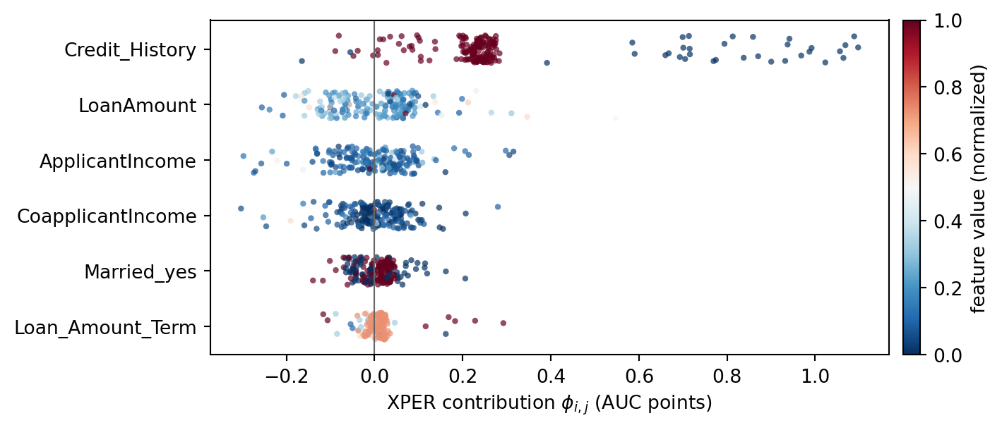
```{python}
#| label: xper-beeswarm
#| fig-cap: "Per-observation XPER values. Horizontal spread at a given feature row shows how heterogeneously that feature contributes across borrowers."
# The upstream XPER beeswarm viz reuses SHAP's internals with a stale API.
# Plot individual_phi directly: feature rows vs borrower points, colored by
# the feature value (same semantics as a SHAP beeswarm).
ind_phi = np.asarray(individual_phi)[:, 1:]
labels = list(X.columns)
p = ind_phi.shape[1]
order = np.argsort(np.abs(ind_phi).mean(axis=0))[::-1]
fig, ax = plt.subplots(figsize=(7.5, 0.35 * p + 1.2))
rng = np.random.default_rng(0)
for row, j in enumerate(order):
    phi_j = ind_phi[:, j]
    x_j = X_te.iloc[:, j].to_numpy(dtype=float)
    x_norm = (x_j - x_j.min()) / (np.ptp(x_j) + 1e-12)
    jitter = rng.uniform(-0.25, 0.25, size=phi_j.shape[0])
    ax.scatter(phi_j, np.full_like(phi_j, row) + jitter,
               c=x_norm, cmap="RdBu_r", s=10, alpha=0.7, linewidths=0)
ax.axvline(0, color="0.4", lw=0.8)
ax.set_yticks(range(p))
ax.set_yticklabels([labels[j] for j in order])
ax.invert_yaxis()
ax.set_xlabel(r"XPER contribution $\phi_{i,j}$ (AUC points)")
sm = plt.cm.ScalarMappable(cmap="RdBu_r",
                           norm=plt.Normalize(vmin=0, vmax=1))
sm.set_array([])
cbar = fig.colorbar(sm, ax=ax, fraction=0.025, pad=0.02)
cbar.set_label("feature value (normalized)")
plt.tight_layout()
plt.show()
```
The beeswarm is where XPER and SHAP diverge in interpretation. A SHAP beeswarm reads as "how does feature $j$ move individual predictions?" The XPER beeswarm reads as "how does feature $j$ contribute to correctly *ranking defaulters above non-defaulters* for this particular borrower?" Points with $\phi_{i,j}<0$ are observations where feature $j$ actively *hurts* the model's AUC contribution, typically mis-signed WoE relationships or interaction masks.
### Local view: one borrower
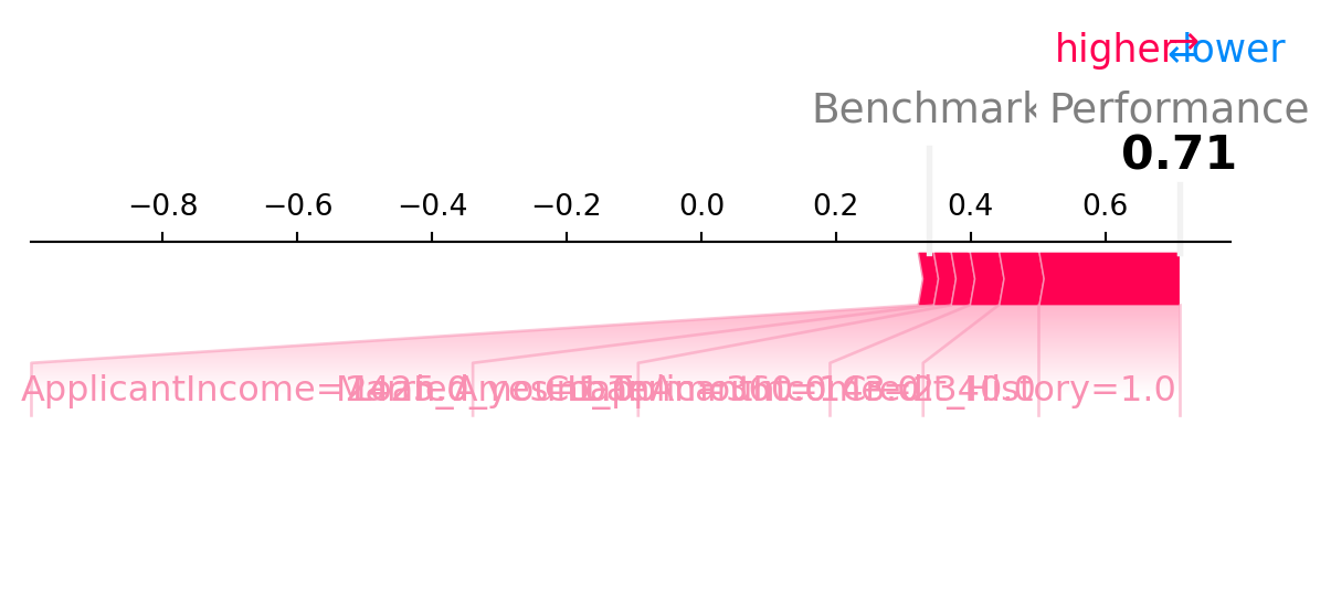
```{python}
#| label: xper-force
#| fig-cap: "Individual XPER force plot for a single test applicant. $\\phi_{i,0}$ anchors at the random benchmark; each feature pushes the applicant's AUC-contribution up or down."
viz.force_plot(
    XPER_values=(global_phi, individual_phi),
    instance=0, X_test=X_te,
    variable_name=list(X.columns),
)
plt.show()
```
## Segmentation by XPER profile {#sec-xper-segmentation}
Individual XPER vectors $\phi_i\in\mathbb{R}^{q+1}$ describe *how each borrower's performance contribution is structured across features*. Borrowers with similar $\phi_i$ are those for whom the model's discriminatory power flows through the same features. The paper shows that clustering on $\phi_i$ and fitting one model per cluster improves global AUC beyond what any single global model achieves, without new features.
The intuition: a pooled model must compromise between subpopulations whose optimal feature weightings differ. Feature-importance clustering (e.g. on SHAP) captures how predictions vary; XPER clustering captures how *performance* varies, which is the objective that refitting optimizes.
```{python}
#| label: xper-segmentation
from sklearn.cluster import KMeans
from sklearn.linear_model import LogisticRegression
from sklearn.metrics import roc_auc_score

Phi = np.asarray(individual_phi)
if Phi.shape[1] == len(X.columns) + 1:
    Phi = Phi[:, 1:]

km = KMeans(n_clusters=2, n_init=10, random_state=42).fit(Phi)
groups_te = km.labels_

# assign each training row to the nearest test-set cluster centroid
# in the model's own feature space (proxy: score-rank deciles) for illustration
tr_scores = clf.predict_proba(X_tr)[:, 1]
te_scores = clf.predict_proba(X_te)[:, 1]
cut = np.quantile(te_scores, 0.5)
groups_tr = (tr_scores > cut).astype(int)

segment_auc = []
for g in np.unique(groups_te):
    mask_tr = groups_tr == g
    mask_te = groups_te == g
    if mask_tr.sum() < 50 or mask_te.sum() < 20:
        continue
    seg = LogisticRegression(max_iter=1000).fit(X_tr[mask_tr], y_tr[mask_tr])
    p   = seg.predict_proba(X_te[mask_te])[:, 1]
    segment_auc.append((g, mask_te.sum(), roc_auc_score(y_te[mask_te], p)))

pd.DataFrame(segment_auc, columns=["cluster", "n_test", "segment_AUC"])
```
In production the segmentation step would be embedded in a cross-validated wrapper: cluster on training-set XPER values, assign test rows by nearest centroid, fit per-cluster estimators, and pool back to a global AUC with inverse-propensity weights. The paper reports a meaningful AUC gain on an auto-loan portfolio; the gain in consumer credit tends to be smaller but still material when the portfolio mixes thin-file and thick-file borrowers.
## When to reach for XPER
Use XPER, not SHAP, when the question is:
- **Which features justify keeping this model in production?** XPER gives AUC-point contributions directly; SHAP does not.
- **Can we prune features without hurting discrimination?** A feature with $\phi_j\approx 0$ and small variance in $\phi_{i,j}$ is a pruning candidate. SHAP would flag features whose *predictions* move little, which is not the same.
- **Is population heterogeneity worth exploiting with segment models?** Cluster $\phi_i$; if clusters separate, segment.
- **Does a regulator-chosen metric (balanced accuracy, Brier under class-imbalance weights, custom cost-weighted loss) decompose cleanly?** XPER is metric-agnostic as long as @eq-additive-metric holds.
Use SHAP, not XPER, when the question is about a single adverse-action notice, a counterfactual, or feature-level calibration of probabilities. The two are complements: store both alongside the scored row in the feature store.
## Limits and caveats
- **Marginal vs conditional reference.** Like Kernel SHAP, `XPER` marginalizes over the empirical joint of the background features, not the conditional given the coalition. Under strong feature dependence this can attribute performance to features whose information is redundant with already-included ones. Conditional XPER is a research direction; in practice report correlations alongside $\phi_j$.
- **Metric choice is a modeling choice.** Ranking metrics (AUC) and calibration metrics (Brier) can assign materially different $\phi_j$ to the same feature. A feature that improves ordering but distorts probabilities will look valuable under AUC-XPER and destructive under Brier-XPER. Report both.
- **Sampling variance.** With `kernel=True` and finite background samples, $\hat\phi_j$ carries Monte Carlo error. The paper establishes $\sqrt n$-consistency and asymptotic normality under regularity (see Appendix of @hue2023xper); practically, run two seeds and report a range.
- **No causal content.** XPER explains a *model's* performance, not the data-generating process. A feature that proxies for a protected attribute can dominate $\phi_j$; that is a fairness finding, not a causal claim. See @sec-ch23.
## Vietnam and emerging markets
### Market context
XPER was introduced at a time when European and US banks had already validated Shapley-based explainers under SR 11-7 and Article 22 regimes. Vietnamese banks operate in a different validation setting. The State Bank of Vietnam supervises model risk through Circular 13/2018 on internal control systems and through the capital framework implemented in Circular 41/2016, as amended by Circular 22/2023/TT-NHNN (29 Dec 2023) on capital adequacy ratios [@sbv_circular22_2023]. Neither circular prescribes a performance-attribution method. The Credit Information Center covers roughly half of the adult population [@cic_vietnam2023], and fintech lenders rely on alternative signals from mobile money, telco top-ups, and merchant networks. In that setting, the cost of each feature is visible, because data-sharing agreements and vendor fees are priced per record per month.
### Application considerations
Feature cost is where XPER earns its place. A Vietnamese lender that pays a monthly subscription to a telco data provider, a wallet aggregator, and the bureau must decide which subscriptions to renew. SHAP does not answer that question. It tells you which features move individual probabilities, not which features produce the aggregate AUC that justifies the vendor fee. XPER does. A feature whose AUC contribution is smaller than its monthly per-application cost times the application volume is a feature to prune at renewal. The same argument applies to internal feature engineering: a Polars pipeline that consumes fifteen minutes of batch time to build a derived feature whose XPER contribution is two basis points of AUC is a pipeline to retire.
### Rationalization
The second use of XPER in Vietnam is audit defense. When the SBV examines a bank's internal model, the examiner reads the validation file. A validation file that lists features and their marginal AUC contributions, traced to a stable estimator, is easier to defend than a file that lists only SHAP beeswarm plots. The XPER report also supports the ESG disclosure that larger Vietnamese banks publish under voluntary IFC standards, because it quantifies the model's dependence on features that are either socially sensitive (gender, region) or environmentally correlated (agricultural sector exposure). A segment-clustering extension of XPER, as in @hue2023xper, also helps identify borrower clusters whose model is weaker. For a lender expanding from urban prime to rural thin-file customers, this points to where the next model iteration must be focused.
### Practical notes
Use XPER alongside SHAP, not in place of it. Pin the `XPER` package version in an internal wheel mirror. Compute AUC-XPER and Brier-XPER and report both. For features tied to Lunar New Year seasonality, compute XPER on a full-year window to avoid spurious attributions. Combine the XPER report with a feature-cost table maintained by procurement. When the reported AUC contribution of a vendor feature drops below its amortized cost, flag the feature for a renegotiation conversation. For segment-specific XPER, cluster borrowers by urban versus rural and by bureau-file versus thin-file, because the feature set that carries AUC in one segment rarely carries it in the other. Document the background distribution and the reference sample; in a Vietnamese data center the background draw from a random day will produce different attributions than a background that respects the Lunar New Year payment cycle.
## Summary
XPER turns the Shapley machinery outward: instead of decomposing $f(x)-\mathbb{E}[f(X)]$ for one borrower, it decomposes $\mathrm{PM}-\phi_0$ for the whole test sample, with per-observation decompositions as a byproduct. The package wraps the estimator, the kernel approximation, and three visualizations; the math is the Shapley value applied to a different coalition game; the practical payoff is a feature-level attribution of AUC (or any additive metric) that regulators can read line-by-line and that modelers can use to prune, segment, and re-fit.