---
execute:
echo: true
eval: true
warning: false
message: false
---
# Algorithmic Fairness: Theory and Definitions {#sec-ch23}
::: {.callout-note appearance="simple" icon="false"}
**Scope: both retail and corporate.** Fairness definitions (demographic parity, equalized odds, calibration) under ECOA Regulation B, which covers consumer and small-business credit. Most worked theory and applied work is on consumer; small-business fairness is touched on and developed empirically in @sec-ch24.
:::
## Overview {.unnumbered}
A credit scoring model is a policy. It decides who gets a loan, what rate, what limit, and who gets told no. Regulators, courts, and borrowers have been arguing about how to audit that policy for decades. The argument has sharpened since machine learning replaced linear scorecards. A neural network does not explain itself the way a weight-of-evidence card does, and the training data carries the discrimination of history. That is the setting of this chapter.
Fairness is not a single objective. It is a family of competing objectives, each defensible, each mutually inconsistent with the others once base rates across groups differ. Practitioners who do not see this collision spend years chasing one metric, reporting success, and discovering later that they have made another metric worse. The impossibility results of @chouldechova2017fair and @kleinberg2017inherent formalize the collision. They also bound what a technical fix can deliver. Everything in this chapter either leads up to those theorems or lives in their shadow.
A second audience reads this chapter from outside the US and EU. Most emerging-market lenders operate under no disparate-impact doctrine at all. The fairness question is still live, but its teeth come from reputational risk, ESG disclosure, and parent-group policy, not from a federal examiner. We treat that setting explicitly in the Vietnam and emerging markets section later in this chapter, because the mathematical taxonomy here travels across legal regimes, while the enforcement model does not.
The chapter is built in three passes. First, the legal frame that governs lending in the United States and Europe (@sec-ch23), because fairness definitions without legal mapping are a toy. Second, the mathematical taxonomy: demographic parity (@sec-ch23-parity), conditional parity (@sec-ch23-cond-parity), equalized odds (@sec-ch23-eqodds), calibration (@sec-ch23-calib), counterfactual fairness (@sec-ch23-cf). Third, the three intervention families (pre-processing (@sec-ch23-preproc), in-processing (@sec-ch23-inproc), post-processing (@sec-ch23-postproc)) with enough code to reproduce each one on a simulated portfolio. @sec-ch24 handles the empirical follow-through on real data.
### Notation {.unnumbered}
Let $Y \in \{0, 1\}$ be the binary outcome (one denotes default), $\hat{Y} \in \{0, 1\}$ the model's binary decision (one denotes "deny credit" when we are explicit about the lending convention, or "predict default"), $S \in [0, 1]$ the continuous score (higher means riskier), $A \in \{0, 1\}$ a protected attribute (zero is the reference group, one the "minority" group), and $X$ the feature vector used by the model. When results generalize to $A$ taking more than two values we say so.
---
## Protected attributes in credit: the legal frame {#sec-ch23-fairtheory}
### ECOA and Regulation B
The United States lists prohibited bases for credit discrimination in the Equal Credit Opportunity Act (15 U.S.C. 1691) and its implementing rule, Regulation B (12 C.F.R. Part 1002). The prohibited bases are race, color, religion, national origin, sex, marital status, age (provided the applicant has capacity to contract), receipt of income from a public assistance program, and good-faith exercise of rights under the Consumer Credit Protection Act. Regulation B, section 1002.4(a), states the general prohibition: a creditor shall not discriminate against an applicant on a prohibited basis regarding any aspect of a credit transaction.
Two doctrines govern enforcement. The first is disparate treatment: treating an applicant differently because of a protected characteristic. The second is disparate impact: a facially neutral policy that produces a disproportionate adverse effect on a protected class and is not justified by business necessity. The Supreme Court endorsed disparate impact in housing credit in Texas Department of Housing v. Inclusive Communities Project (2015). The Consumer Financial Protection Bureau applies both doctrines to lending under ECOA.
A model that uses $A$ as an input produces disparate treatment by construction. A model that excludes $A$ but leans on proxies can still produce disparate impact. Neither doctrine tolerates "blind" models that achieve parity of outcomes by coincidence. Both require documentation.
### The four-fifths rule
The four-fifths rule is a rule of thumb, not a statute. It comes from the 1978 Uniform Guidelines on Employee Selection Procedures (29 C.F.R. Part 1607.4(D)) issued jointly by the EEOC, DOL, DOJ, and OPM. Lending regulators have borrowed it as a screening device, not a safe harbor.
Let $p_a = \Pr(\hat{Y} = 1 \mid A = a)$ be the positive-prediction rate in group $a$ (in lending, this is the approval rate). The four-fifths rule flags a policy if the minority approval rate is less than 80 percent of the majority approval rate:
$$
\frac{\min_a p_a}{\max_a p_a} < 0.80.
$$ {#eq-fourfifths}
The rule flags a ratio, not a difference. It tolerates absolute gaps at low selection rates and penalizes them at high rates. It is silent on sample size, which is why EEOC guidance says to combine it with statistical tests of significance.
Practitioners who have sat in a regulatory examination know that the four-fifths number is the first thing anyone computes. It is also the first thing defense counsel will try to rebut with a business-necessity argument. The rest of this chapter is about what comes after you have computed it.
### Europe and beyond
The EU operates under the Race Equality Directive (2000/43/EC), the Gender Goods and Services Directive (2004/113/EC, which generally prohibits using sex as a pricing factor), and the GDPR (Regulation 2016/679), whose Article 22 gives data subjects the right not to be subject to a decision based solely on automated processing if it produces legal effects. The EU AI Act (Regulation 2024/1689, entered into force August 2024) classifies credit scoring as a high-risk AI system under Annex III, point 5(b), and imposes obligations on data governance, bias mitigation, and post-market monitoring.
The chapter's math is jurisdiction-agnostic. The enforcement practice is not. A model that passes U.S. review can still fail an EU conformity assessment because the EU framework emphasizes ex ante documentation of data quality and risk management under Article 9, while U.S. practice emphasizes ex post statistical evidence of adverse impact.
### Why "protected" is harder than it sounds
ECOA forbids using race. U.S. mortgage lenders collect race because HMDA requires it. U.S. credit-card issuers cannot collect race directly. They infer it, for fair-lending purposes only, with the Bayesian Improved Surname Geocoding (BISG) procedure of Elliott et al. (2009), which combines surname lists from the Census with tract-level demographics. BISG is inaccurate at the individual level, which complicates any fairness audit that conditions on $A$. @sec-ch24 returns to this.
Age is nominally protected but must be allowed to enter a model in some form, because creditworthiness depends on repayment history, which depends on age. The regulatory accommodation is that age can be used if it does not disadvantage an applicant aged 62 or older, and it must enter as a continuous or carefully binned variable, not as a discriminating threshold. See 12 C.F.R. 1002.6(b)(2).
---
## Formal setup
A credit model is a predictor $f: \mathcal{X} \to [0, 1]$ that outputs a score $S = f(X)$. A decision rule is a threshold policy $\hat{Y} = \mathbb{1}[S > t]$, possibly with group-dependent thresholds $t_a$. Data is drawn i.i.d. from a joint distribution $\mathcal{D}$ over $(X, A, Y)$.
We write $P_a(\cdot) = \Pr(\cdot \mid A = a)$ for conditional probabilities in group $a$, and use $E_a[\cdot]$ similarly. The base rate in group $a$ is $\pi_a = P_a(Y = 1) = \Pr(Y = 1 \mid A = a)$. The critical empirical fact that drives most of what follows: in virtually every consumer-credit portfolio, $\pi_a$ differs across groups.
With that setup, we can enumerate the formal definitions.
### Statistical (demographic) parity {#sec-ch23-parity}
A predictor satisfies demographic parity with respect to $A$ if
$$
P_0(\hat{Y} = 1) = P_1(\hat{Y} = 1).
$$ {#eq-dp}
Equivalently, $\hat{Y} \perp A$: the decision is statistically independent of the protected attribute. The relaxed $\varepsilon$-form is
$$
\lvert P_0(\hat{Y} = 1) - P_1(\hat{Y} = 1) \rvert \le \varepsilon,
$$ {#eq-dpeps}
with $\varepsilon = 0$ being strict parity and the four-fifths rule corresponding to the ratio version $P_1(\hat{Y}=1) / P_0(\hat{Y}=1) \ge 0.8$ (after labeling the majority as group zero).
Demographic parity is the oldest formal definition. It is intuitive and easy to test. It has two serious problems. First, it ignores $Y$: a policy that approves everyone is perfectly parity-compliant. Second, when $\pi_0 \neq \pi_1$, demographic parity forces the accuracy to drop in at least one group. The policy must systematically approve more of the worse-risk group or deny more of the better-risk group than the data would suggest.
@dwork2012fairness argued that demographic parity conflates "fair" with "identical," and proposed a "fairness through awareness" framework based on Lipschitz continuity in a task-specific similarity metric: individuals who are similar with respect to the task should receive similar predictions. The framework is mathematically clean and rarely operational, because the similarity metric is never known.
### Conditional statistical parity {#sec-ch23-cond-parity}
A predictor satisfies conditional statistical parity relative to a set of legitimate risk factors $L \subseteq X$ if
$$
P_0(\hat{Y} = 1 \mid L = \ell) = P_1(\hat{Y} = 1 \mid L = \ell) \quad \text{for all } \ell.
$$ {#eq-cdp}
This is the "business necessity" version: once you control for $L$, the residual disparity should be zero. The catch is that the analyst picks $L$. Choose $L$ to include every variable correlated with $Y$, and conditional parity collapses to "the model is well-specified." Choose $L$ sparely, and the constraint approaches demographic parity.
### Equalized odds and equal opportunity {#sec-ch23-eqodds}
@hardt2016equality defined equalized odds: $\hat{Y}$ satisfies equalized odds with respect to $A$ and $Y$ if
$$
P_0(\hat{Y} = 1 \mid Y = y) = P_1(\hat{Y} = 1 \mid Y = y) \quad \text{for } y \in \{0, 1\}.
$$ {#eq-eo}
The constraint is $\hat{Y} \perp A \mid Y$. Unpacking, that is two equalities: the true-positive rate (TPR) matches across groups, and the false-positive rate (FPR) matches across groups. Equivalently in lending terms, the approval rate among repayers is equal, and the approval rate among defaulters is equal.
Equal opportunity is the one-sided relaxation that drops the $y = 0$ constraint and keeps only
$$
P_0(\hat{Y} = 1 \mid Y = 1) = P_1(\hat{Y} = 1 \mid Y = 1).
$$ {#eq-eop}
For defaults this says: among the people who would actually default, the flag rate is equal across groups. The asymmetric version privileges the "positive" outcome label, which in credit is awkward because we relabel in @sec-ch23-simulation-setup.
Equalized odds is error-rate parity. It is the criterion most consistent with the intuition of Title VII disparate-treatment jurisprudence: holding outcome constant, the probability of the decision should not depend on group membership.
### Predictive equality
Predictive equality is the $y = 0$ branch of equalized odds:
$$
P_0(\hat{Y} = 1 \mid Y = 0) = P_1(\hat{Y} = 1 \mid Y = 0).
$$ {#eq-pe}
In lending this is: the false-positive (wrongful-denial) rate is equal across groups. @chouldechova2017fair used this definition in her analysis of recidivism prediction, because she and ProPublica argued that the disparity the journalism uncovered was a disparity in false-positive rates among Black defendants.
### Calibration by group {#sec-ch23-calib}
Calibration says that the score means what it says it means. Formally,
$$
P(Y = 1 \mid S = s, A = a) = s \quad \text{for all } s, a.
$$ {#eq-cal}
Calibration by group is the same condition but stated per group. When a lender is calibrated by group, a 10 percent default probability from the score corresponds to a 10 percent observed default rate, within each group separately.
A weaker but frequently used condition is "predictive parity" or "sufficiency," which requires
$$
P_0(Y = 1 \mid \hat{Y} = y) = P_1(Y = 1 \mid \hat{Y} = y) \quad \text{for } y \in \{0, 1\},
$$ {#eq-pp}
i.e., the positive predictive value and negative predictive value are equal across groups. This is the condition that the COMPAS vendor Northpointe defended itself with in the ProPublica debate.
Group calibration and predictive parity are related but not identical: predictive parity is equality across groups of the posterior probability of $Y$ given the binary decision, while calibration requires correctness of posterior probability of $Y$ given the score at every level.
### Counterfactual fairness {#sec-ch23-cf}
Counterfactual fairness [@kusner2017counterfactual] asks that the prediction be the same in the actual world and in a counterfactual world in which the individual had belonged to a different protected group, with all downstream effects propagated through a structural causal model.
Let $\mathcal{M}$ be a structural causal model over $(A, X, Y)$, and write $X_{A \leftarrow a}(u)$ for the counterfactual value of $X$ when $A$ is set to $a$ and the background noise $u$ is fixed. A predictor $\hat{Y}$ is counterfactually fair if
$$
\Pr\bigl(\hat{Y}_{A \leftarrow a}(u) = y \mid X = x, A = a'\bigr) = \Pr\bigl(\hat{Y}_{A \leftarrow a''}(u) = y \mid X = x, A = a'\bigr)
$$ {#eq-cf}
for all $y$, $a$, $a''$, and observable $(x, a')$. The condition is easier to parse on a causal diagram: $\hat{Y}$ must be a function of variables that are not descendants of $A$ in the DAG.
The practical payload of counterfactual fairness is a recipe: identify the DAG, find the non-descendants of $A$, fit the model only on those. In consumer credit, very little is a non-descendant of race in the U.S. context because race affects neighborhood, which affects schools, which affects income, which affects savings, which affects FICO. Counterfactual fairness without a willing interpretation of the DAG is restrictive to the point of unusability. @kilbertus2017avoiding extend the analysis and distinguish resolving from non-resolving variables, which softens the rigidity but requires the same DAG commitment.
---
## Derivations
### Equalized odds from mutual information
Equalized odds says $\hat{Y} \perp A \mid Y$. By the chain rule for mutual information,
$$
I(\hat{Y}; A) = I(\hat{Y}; A \mid Y) + I(\hat{Y}; Y) - I(\hat{Y}; Y \mid A).
$$
The first term is zero under equalized odds. The remaining two capture the "information about $A$ inside the prediction that flows through $Y$." Equalized odds therefore still permits disparity in $\hat{Y}$ when $Y$ itself is correlated with $A$. This is why equalized odds is compatible with a disparate approval rate.
### Hardt threshold adjustment as a linear program
The $ROC_a$ curve for a scored group $a$ is the set $\{(\mathrm{FPR}_a(t), \mathrm{TPR}_a(t)) : t \in [0, 1]\}$. The convex hull of $ROC_a$ with the points $(0,0)$ and $(1,1)$, denoted $\mathrm{conv}(ROC_a)$, is the achievable set of $(\mathrm{FPR}, \mathrm{TPR})$ pairs for group $a$ using deterministic and randomized threshold rules on the existing score.
The post-processing problem of @hardt2016equality is: find decision rules $D_0$ for group $0$ and $D_1$ for group $1$, each of which is a (randomized) threshold on the score, such that $(\mathrm{FPR}_{D_0}, \mathrm{TPR}_{D_0}) = (\mathrm{FPR}_{D_1}, \mathrm{TPR}_{D_1}) = (u, v)$ for some common $(u, v) \in \mathrm{conv}(ROC_0) \cap \mathrm{conv}(ROC_1)$, and the common operating point maximizes expected utility.
Let the utility of the decision $\hat{Y}$ given label $Y$ be $U_{11}, U_{10}, U_{01}, U_{00}$ for the four cells. Expected utility given $(u, v)$ in group $a$ is
$$
\mathcal{U}_a(u, v) = \pi_a \bigl[U_{11} v + U_{01} (1 - v)\bigr] + (1 - \pi_a) \bigl[U_{10} u + U_{00} (1 - u)\bigr].
$$ {#eq-utility}
With group weights $w_a = \Pr(A = a)$, total expected utility is $\sum_a w_a \mathcal{U}_a(u, v)$, which is linear in $(u, v)$. The constraint set $\mathrm{conv}(ROC_0) \cap \mathrm{conv}(ROC_1)$ is a convex polygon. Hence the Hardt problem is a linear program:
$$
\begin{aligned}
\max_{u, v} \quad & w_0 \mathcal{U}_0(u, v) + w_1 \mathcal{U}_1(u, v) \\
\text{s.t.} \quad & (u, v) \in \mathrm{conv}(ROC_0) \cap \mathrm{conv}(ROC_1).
\end{aligned}
$$ {#eq-lp}
For equal opportunity (TPR parity only) the intersection is replaced by the slab $\{(u_0, v, u_1, v)\}$, which is still a polyhedron. The solution recipe is to enumerate vertices of the two ROC convex hulls, form the intersection polygon, and pick the vertex or edge that maximizes the linear objective. In practice `fairlearn.postprocessing.ThresholdOptimizer` solves this by interpolating between two threshold operating points per group with a Bernoulli coin, which is exactly what the randomized-threshold interpretation requires.
The post-processing solution is Pareto optimal on the group-specific ROC curves: you cannot dominate it without violating either equalized odds or the LP optimality.
### Lagrangian formulation for fairness-constrained ERM
The in-processing strategy of @agarwal2018reductions treats fairness as a linear constraint on the empirical risk. Let $\mathcal{F}$ be a hypothesis class, $R(f) = E[\ell(f(X), Y)]$ the risk, and $M$ a finite set of linear constraints encoding a fairness notion (for equalized odds, four linear equalities balancing TPR and FPR across groups, turned into a signed $2|\mathcal{A}|$ constraint vector). The problem is
$$
\min_{f \in \mathcal{F}} R(f) \quad \text{s.t.} \quad M\gamma(f) \le c,
$$ {#eq-constr}
where $\gamma(f) = (\gamma_j(f))_j$ is the vector of group-conditional moment functionals. The Lagrangian is
$$
\mathcal{L}(f, \lambda) = R(f) + \lambda^{\top}(M\gamma(f) - c),
$$ {#eq-lagrangian}
with $\lambda \ge 0$. The dual problem, $\max_{\lambda \ge 0} \min_{f} \mathcal{L}(f, \lambda)$, has a saddle point because both the primal objective and the constraint functionals are linear in the distribution of $f$ (after randomization over $\mathcal{F}$). @agarwal2018reductions solve it by no-regret iteration: the $\lambda$-player updates by exponentiated gradient, and the $f$-player responds by cost-sensitive classification with example weights $1 + \lambda^{\top} m_i$, where $m_i$ is the row of $M$ corresponding to observation $i$. The exponentiated-gradient reduction turns any weighted-ERM classifier into a fair classifier up to slack $\varepsilon$. `fairlearn.reductions.ExponentiatedGradient` implements this.
### Proof sketch of the impossibility theorem
The cleanest version of the impossibility result is the one in @kleinberg2017inherent. We reproduce the essentials.
Let $S$ be a score, $A \in \{0, 1\}$ a protected attribute, $Y \in \{0, 1\}$ an outcome. Define three desiderata.
(C1) Calibration within groups: for each $a$, $E[Y \mid S = s, A = a] = s$ for every score $s$ in the support.
(C2) Balance for the positive class: $E[S \mid Y = 1, A = 0] = E[S \mid Y = 1, A = 1]$.
(C3) Balance for the negative class: $E[S \mid Y = 0, A = 0] = E[S \mid Y = 0, A = 1]$.
Claim. If $\pi_0 \neq \pi_1$ and $Y$ is not a perfect function of $S$ and $A$ (i.e., the score is not a perfect predictor), then (C1), (C2), (C3) cannot all hold simultaneously.
Proof sketch. Under (C1), calibration implies $E[S \mid A = a] = E[Y \mid A = a] = \pi_a$. Under (C2) and (C3), the conditional means of $S$ within $\{Y = 1\}$ and $\{Y = 0\}$ are equal across groups. Call these common values $\mu_1$ and $\mu_0$. Then
$$
\pi_a = E[S \mid A = a] = \pi_a \mu_1 + (1 - \pi_a) \mu_0
$$
by the law of total expectation. Rearranging,
$$
\pi_a (1 - \mu_1 + \mu_0) = \mu_0,
$$
which means the left side is the same across $a$ only if $\pi_0 = \pi_1$ or $\mu_1 - \mu_0 = 1$. The first contradicts different base rates, and the second forces $\mu_1 = 1$ and $\mu_0 = 0$, i.e., a perfect predictor. Neither is allowed under the hypothesis, so at least one of (C1), (C2), (C3) fails.
@chouldechova2017fair proved the equivalent result in a different notation. When one requires simultaneously: predictive parity (equal positive predictive value across groups), equal false-positive rate, and equal false-negative rate, then base-rate equality is implied. Contrapositive: if base rates differ, all three cannot hold. The derivation follows from the identity
$$
\mathrm{FPR}_a = \frac{\pi_a}{1 - \pi_a} \cdot \frac{1 - \mathrm{PPV}_a}{\mathrm{PPV}_a} \cdot \mathrm{TPR}_a,
$$
which links false-positive rate, true-positive rate, predictive value, and prevalence.
This is not a curiosity. It is the load-bearing wall under every fair-lending debate. The minute a lender publishes parity on any two of {calibration, TPR, FPR}, and base rates differ, the third is forced to disagree.
---
## Simulation setup {#sec-ch23-simulation-setup}
We build a synthetic loan dataset with known ground truth so the fairness geometry is transparent. Real data appears in @sec-ch24.
```{python}
#| label: setup
import warnings
warnings.filterwarnings("ignore")
import sys
sys.path.insert(0, '../code')

import numpy as np
from creditutils import stable_sigmoid
import pandas as pd
import matplotlib.pyplot as plt
from sklearn.linear_model import LogisticRegression
from sklearn.model_selection import train_test_split
from sklearn.metrics import roc_auc_score, roc_curve
from sklearn.calibration import calibration_curve

from fairlearn.postprocessing import ThresholdOptimizer
from fairlearn.metrics import (
    MetricFrame,
    demographic_parity_difference,
    equalized_odds_difference,
    selection_rate,
    true_positive_rate,
    false_positive_rate,
    false_negative_rate,
)

RNG = np.random.default_rng(20240416)
np.random.seed(42)
```
```{python}
#| label: simulate
def simulate_loans(n=12000, seed=0):
    rng = np.random.default_rng(seed)
    # protected attribute A: 0 = majority (60%), 1 = minority (40%)
    A = (rng.uniform(size=n) < 0.4).astype(int)
    # latent creditworthiness z shifted by group; group 1 has lower mean
    z = rng.normal(0, 1, n) - 0.8 * A
    # default probability (higher z means safer, so lower default)
    lin = -0.6 - 1.3 * z
    p_default = stable_sigmoid(lin)
    Y = (rng.uniform(size=n) < p_default).astype(int)
    # observable features: noisy proxies of z plus a group-leaking feature
    x1 = z + rng.normal(0, 0.5, n)      # strong, mostly about risk
    x2 = z + rng.normal(0, 0.7, n)      # weaker
    x3 = 0.4 * A + rng.normal(0, 1, n)  # leaks group membership
    # socioeconomic proxy highly correlated with A
    x4 = 0.7 * A + 0.3 * rng.normal(0, 1, n)
    return pd.DataFrame({
        "x1": x1, "x2": x2, "x3": x3, "x4": x4,
        "A": A, "Y": Y
    })

df = simulate_loans(n=12000, seed=0)
print(df.groupby("A")["Y"].agg(["mean", "count"]).rename(columns={"mean": "base_rate"}))
```
We have a clear difference in base rates: group 0 has lower default probability than group 1. Group 1 is also over-represented in the high-$x_4$ region, which a naive model will interpret as a risk signal.
### Baseline logistic regression and the fairness metrics
```{python}
#| label: fit-baseline
feat_cols = ["x1", "x2", "x3", "x4"]
X = df[feat_cols].values
Y = df["Y"].values
A = df["A"].values

Xtr, Xte, ytr, yte, Atr, Ate = train_test_split(
    X, Y, A, test_size=0.3, random_state=42, stratify=Y
)

base_lr = LogisticRegression(max_iter=500).fit(Xtr, ytr)
p_hat = base_lr.predict_proba(Xte)[:, 1]
y_hat = (p_hat > 0.5).astype(int)

print(f"AUC (overall):           {roc_auc_score(yte, p_hat):.3f}")
print(f"AUC (group 0):           {roc_auc_score(yte[Ate==0], p_hat[Ate==0]):.3f}")
print(f"AUC (group 1):           {roc_auc_score(yte[Ate==1], p_hat[Ate==1]):.3f}")
print()
print(f"Base rate (group 0):     {yte[Ate==0].mean():.3f}")
print(f"Base rate (group 1):     {yte[Ate==1].mean():.3f}")
print()
print(f"Statistical parity diff:      {demographic_parity_difference(yte, y_hat, sensitive_features=Ate):+.3f}")
print(f"Equalized odds diff:          {equalized_odds_difference(yte, y_hat, sensitive_features=Ate):+.3f}")
```
`MetricFrame` shows rate decomposition per group.
```{python}
#| label: metricframe-base
metrics = {
    "selection_rate":     selection_rate,
    "TPR":                true_positive_rate,
    "FPR":                false_positive_rate,
    "FNR":                false_negative_rate,
}
mf = MetricFrame(metrics=metrics, y_true=yte, y_pred=y_hat, sensitive_features=Ate)
print(mf.by_group.round(3))
print()
print(mf.difference(method="between_groups").round(3))
```
The baseline exhibits all the canonical problems: the selection rate (predicted default rate) is higher in group 1 because the true default rate is higher, and the TPR/FPR gaps are nontrivial. The four-fifths ratio on the approval side (treating "predict repay" as the favorable outcome):
```{python}
#| label: four-fifths
approve_0 = (y_hat[Ate == 0] == 0).mean()
approve_1 = (y_hat[Ate == 1] == 0).mean()
print(f"Approval rate group 0: {approve_0:.3f}")
print(f"Approval rate group 1: {approve_1:.3f}")
ratio = min(approve_0, approve_1) / max(approve_0, approve_1)
print(f"Four-fifths ratio:     {ratio:.3f}  (threshold 0.80)")
print(f"Flagged:               {ratio < 0.80}")
```
### Calibration by group
Calibration is checked by binning predicted probabilities and comparing to observed default rates within each group.
```{python}
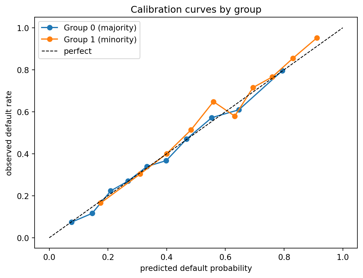
#| label: calibration-by-group
#| fig-cap: "Calibration curves by protected group for the baseline logistic regression."
fig, ax = plt.subplots(figsize=(6.5, 5.0))
for a, label in [(0, "Group 0 (majority)"), (1, "Group 1 (minority)")]:
    mask = Ate == a
    frac_pos, mean_pred = calibration_curve(yte[mask], p_hat[mask], n_bins=10, strategy="quantile")
    ax.plot(mean_pred, frac_pos, "o-", label=label)
ax.plot([0, 1], [0, 1], "k--", lw=1, label="perfect")
ax.set_xlabel("predicted default probability")
ax.set_ylabel("observed default rate")
ax.set_title("Calibration curves by group")
ax.legend()
fig.tight_layout()
plt.show()
```
Logistic regression trained on the pooled sample gives approximately calibrated scores within each group. That is an artifact of the simulation: the latent $z$ is Gaussian within group, and logistic regression is a consistent estimator of the class-posterior under the generated model. Later, when we apply post-processing or adversarial training, calibration will move.
---
## The impossibility theorem in code
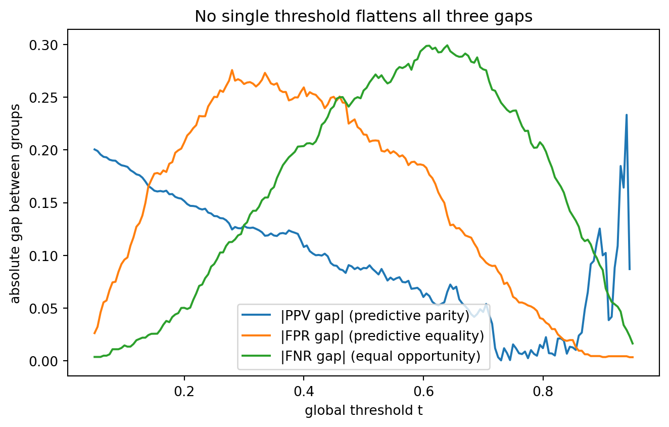
We now construct an empirical demonstration. We take the baseline score and sweep thresholds to find the point that minimizes the calibration-by-group gap, the point that equalizes FPR, the point that equalizes TPR, and show that no single threshold achieves all three.
```{python}
#| label: impossibility-sweep
def group_metrics_at(score, y, a, t):
    yhat = (score > t).astype(int)
    out = {}
    for g in (0, 1):
        m = (a == g)
        yt = y[m]; yh = yhat[m]
        ppv = yh[yh == 1].mean() if (yh == 1).sum() > 0 else np.nan
        # actually PPV = P(Y=1 | yhat=1)
        ppv = yt[yh == 1].mean() if (yh == 1).sum() > 0 else np.nan
        fpr = yh[yt == 0].mean() if (yt == 0).sum() > 0 else np.nan
        fnr = 1 - (yh[yt == 1].mean() if (yt == 1).sum() > 0 else np.nan)
        out[g] = dict(ppv=ppv, fpr=fpr, fnr=fnr)
    return out

ts = np.linspace(0.05, 0.95, 181)
rows = []
for t in ts:
    gm = group_metrics_at(p_hat, yte, Ate, t)
    rows.append({
        "t": t,
        "ppv_gap": abs(gm[0]["ppv"] - gm[1]["ppv"]),
        "fpr_gap": abs(gm[0]["fpr"] - gm[1]["fpr"]),
        "fnr_gap": abs(gm[0]["fnr"] - gm[1]["fnr"]),
    })
sweep = pd.DataFrame(rows)

for col in ["ppv_gap", "fpr_gap", "fnr_gap"]:
    j = sweep[col].idxmin()
    print(f"min {col}: {sweep.loc[j, col]:.3f} at t={sweep.loc[j, 't']:.2f}")
```
```{python}
#| label: impossibility-plot
#| fig-cap: "Three fairness criteria as a function of the global threshold. Each is a different local minimum."
fig, ax = plt.subplots(figsize=(7, 4.5))
ax.plot(sweep["t"], sweep["ppv_gap"], label="|PPV gap| (predictive parity)")
ax.plot(sweep["t"], sweep["fpr_gap"], label="|FPR gap| (predictive equality)")
ax.plot(sweep["t"], sweep["fnr_gap"], label="|FNR gap| (equal opportunity)")
ax.set_xlabel("global threshold t")
ax.set_ylabel("absolute gap between groups")
ax.set_title("No single threshold flattens all three gaps")
ax.legend()
fig.tight_layout()
plt.show()
```
The argmins sit at different thresholds. The impossibility theorem told us this would happen; the sweep makes it visible. A single global threshold cannot simultaneously equate PPV, FPR, and FNR across groups when base rates differ.
A slightly more aggressive demonstration: even if we allow group-specific thresholds, we can only satisfy two of the three criteria at a time. Fix $t_0$ for group 0 and then search $t_1$ in group 1 to equalize FPR and then PPV.
```{python}
#| label: impossibility-group-thresholds
def group_pick_t(score, y, a, t0, match_on="fpr"):
    yhat0 = (score[a == 0] > t0).astype(int)
    y0 = y[a == 0]
    target = {
        "fpr": yhat0[y0 == 0].mean(),
        "tpr": yhat0[y0 == 1].mean(),
        "ppv": y0[yhat0 == 1].mean() if (yhat0 == 1).sum() > 0 else np.nan,
    }[match_on]
    score1 = score[a == 1]; y1 = y[a == 1]
    grid = np.linspace(0.02, 0.98, 961)
    best_t, best_diff = None, np.inf
    for t in grid:
        yh = (score1 > t).astype(int)
        val = {
            "fpr": yh[y1 == 0].mean(),
            "tpr": yh[y1 == 1].mean(),
            "ppv": y1[yh == 1].mean() if (yh == 1).sum() > 0 else np.nan,
        }[match_on]
        if np.isnan(val):
            continue
        d = abs(val - target)
        if d < best_diff:
            best_diff, best_t = d, t
    return best_t, target

t0 = 0.5
t1_fpr, target_fpr = group_pick_t(p_hat, yte, Ate, t0, match_on="fpr")
t1_ppv, target_ppv = group_pick_t(p_hat, yte, Ate, t0, match_on="ppv")
print(f"Match FPR across groups: t0={t0}, t1={t1_fpr:.3f}, FPR target={target_fpr:.3f}")
print(f"Match PPV across groups: t0={t0}, t1={t1_ppv:.3f}, PPV target={target_ppv:.3f}")
print(f"The two thresholds differ, so a lender who fixes t1 to equalize FPR")
print(f"will have a different PPV gap than one who fixes t1 to equalize PPV.")
```
The two "fair" thresholds for group 1 are not the same. Choosing one forces a non-zero residual on the other criterion. That is the impossibility theorem materialized.
---
## Post-processing: Hardt threshold adjustment {#sec-ch23-postproc}
Post-processing operates on a fitted score and produces a new decision rule that satisfies a fairness constraint. The Hardt construction chooses group-specific (randomized) thresholds to land on a common $(FPR, TPR)$ point in the intersection of group-specific ROC convex hulls.
`fairlearn.postprocessing.ThresholdOptimizer` implements this for demographic parity, equalized odds, true-positive-rate parity, and false-positive-rate parity.
```{python}
#| label: threshold-optimizer
to = ThresholdOptimizer(
    estimator=base_lr,
    constraints="equalized_odds",
    objective="accuracy_score",
    prefit=True,
    predict_method="predict_proba",
)
to.fit(Xtr, ytr, sensitive_features=Atr)
y_hat_to = to.predict(Xte, sensitive_features=Ate, random_state=0)

print("After ThresholdOptimizer (equalized_odds):")
mf_to = MetricFrame(metrics=metrics, y_true=yte, y_pred=y_hat_to, sensitive_features=Ate)
print(mf_to.by_group.round(3))
print()
print("Fairness gaps:")
print(f"  statistical parity diff: {demographic_parity_difference(yte, y_hat_to, sensitive_features=Ate):+.3f}")
print(f"  equalized odds diff:     {equalized_odds_difference(yte, y_hat_to, sensitive_features=Ate):+.3f}")
print(f"  original EO diff:        {equalized_odds_difference(yte, y_hat, sensitive_features=Ate):+.3f}")
```
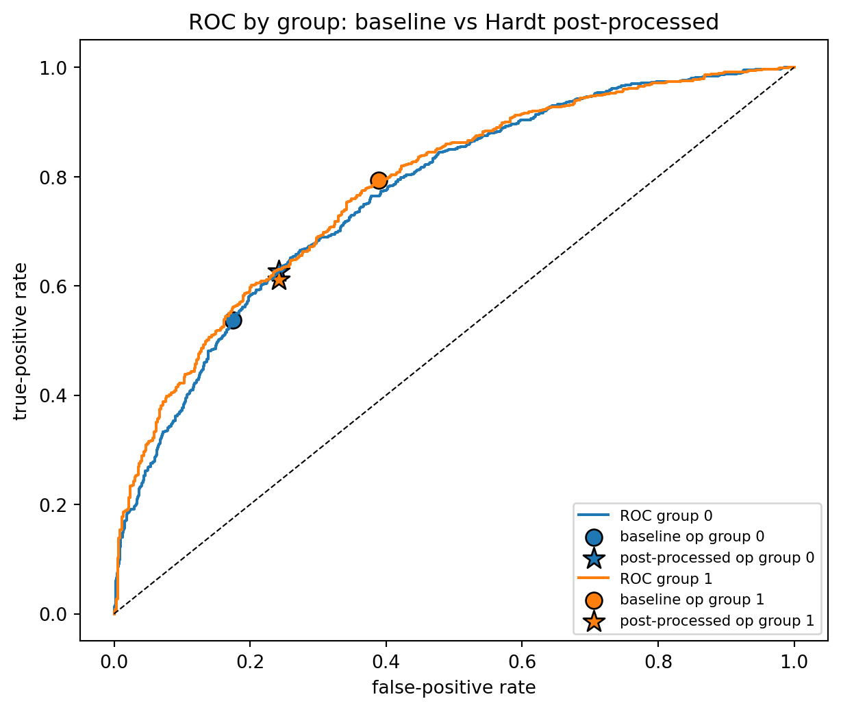
We can also visualize what happened geometrically. The baseline operating point for each group is a single dot; the Hardt solution moves both groups to a common $(FPR, TPR)$ point.
```{python}
#| label: roc-before-after
#| fig-cap: "Group ROC curves with baseline operating points (0.5 threshold) and post-processed common equalized-odds operating point."
fig, ax = plt.subplots(figsize=(6.5, 5.5))
colors = {0: "tab:blue", 1: "tab:orange"}
for g in (0, 1):
    mask = Ate == g
    fpr, tpr, _ = roc_curve(yte[mask], p_hat[mask])
    ax.plot(fpr, tpr, color=colors[g], label=f"ROC group {g}")
    # baseline operating point at t=0.5
    y_g = y_hat[mask]; y_t = yte[mask]
    f = y_g[y_t == 0].mean(); t = y_g[y_t == 1].mean()
    ax.scatter([f], [t], color=colors[g], marker="o", s=80,
               edgecolor="black", label=f"baseline op group {g}")
    # post-processed point
    y_g2 = y_hat_to[mask]
    f2 = y_g2[y_t == 0].mean(); t2 = y_g2[y_t == 1].mean()
    ax.scatter([f2], [t2], color=colors[g], marker="*", s=150,
               edgecolor="black", label=f"post-processed op group {g}")
ax.plot([0, 1], [0, 1], "k--", lw=0.8)
ax.set_xlabel("false-positive rate")
ax.set_ylabel("true-positive rate")
ax.set_title("ROC by group: baseline vs Hardt post-processed")
ax.legend(fontsize=8, loc="lower right")
fig.tight_layout()
plt.show()
```
The post-processed points for the two groups land on top of each other in $(FPR, TPR)$ space, which is the geometric content of equalized odds. The cost is that both groups are moved off their respective ROC curves toward the interior of their convex hull, because the solution is a randomized mixture of two threshold points.
Accuracy also shifts.
```{python}
#| label: accuracy-tradeoff
from sklearn.metrics import accuracy_score
print(f"Accuracy, baseline:       {accuracy_score(yte, y_hat):.3f}")
print(f"Accuracy, post-processed: {accuracy_score(yte, y_hat_to):.3f}")
```
The accuracy drop quantifies the "cost of fairness" in @corbett2017algorithmic: moving the operating point to the common feasible region sacrifices some utility in at least one group. That loss is unavoidable when base rates differ; it is not a flaw of the algorithm.
### What Hardt does not do
Hardt post-processing does not re-calibrate the score. It takes a possibly-calibrated score and produces decision-level parity at the cost of probability-level coherence. After the adjustment, the score no longer has an operationally meaningful probability interpretation unless you recalibrate on top [@pleiss2017fairness formalize the tension]. For credit decisioning this often matters because the score drives pricing, capital, and CECL provisioning, all of which demand a calibrated probability. The implication is that post-processing is best used at the decision layer while keeping an unadjusted probability score for pricing and loss forecasting.
---
## Pre-processing: reweighing and disparate-impact removal {#sec-ch23-preproc}
### Kamiran and Calders reweighing
@kamiran2012data propose a pre-processing weight $w(a, y)$ that makes the training sample look like a world in which $Y \perp A$ while keeping the empirical marginals of $A$ and $Y$ unchanged:
$$
w(a, y) = \frac{\Pr(A = a) \Pr(Y = y)}{\Pr(A = a, Y = y)}.
$$ {#eq-kc-weights}
Apply the weights in any standard learner that accepts sample weights.
```{python}
#| label: reweighing
df_tr = pd.DataFrame({"A": Atr, "Y": ytr})
pA = df_tr["A"].value_counts(normalize=True).to_dict()
pY = df_tr["Y"].value_counts(normalize=True).to_dict()
pAY = (df_tr.groupby(["A", "Y"]).size() / len(df_tr)).to_dict()

def kc_weight(a, y):
    return (pA[a] * pY[y]) / pAY[(a, y)]

w_train = np.array([kc_weight(a, y) for a, y in zip(Atr, ytr)])

lr_rw = LogisticRegression(max_iter=500).fit(Xtr, ytr, sample_weight=w_train)
p_rw = lr_rw.predict_proba(Xte)[:, 1]
y_rw = (p_rw > 0.5).astype(int)

print("Kamiran-Calders reweighing:")
print(f"  AUC:                        {roc_auc_score(yte, p_rw):.3f}")
print(f"  Statistical parity diff:    {demographic_parity_difference(yte, y_rw, sensitive_features=Ate):+.3f}")
print(f"  Equalized odds diff:        {equalized_odds_difference(yte, y_rw, sensitive_features=Ate):+.3f}")
print()
print("Baseline for comparison:")
print(f"  AUC:                        {roc_auc_score(yte, p_hat):.3f}")
print(f"  Statistical parity diff:    {demographic_parity_difference(yte, y_hat, sensitive_features=Ate):+.3f}")
print(f"  Equalized odds diff:        {equalized_odds_difference(yte, y_hat, sensitive_features=Ate):+.3f}")
```
Reweighing is cheap and preserves AUC because it only changes the sample distribution of $(A, Y)$, not of $(X, Y)$. The demographic-parity gap shrinks but does not vanish, because the features $x_3$ and $x_4$ still carry information about $A$. The feature-level leakage has to be closed with a different intervention.
### Feldman disparate-impact remover
@feldman2015certifying proposed to edit each continuous feature so that its distribution conditional on $A$ becomes $A$-invariant, while preserving the marginal ordering within groups.
Let $X_j$ be a continuous feature with group-conditional CDFs $F_{j,a}$, and let $F_j^*$ be a target marginal (for example a weighted mix of the group CDFs). The disparate-impact remover replaces $X_j$ in group $a$ with
$$
\tilde{X}_j = F_j^{*-1}\!\bigl((1 - \lambda) F_{j,a}(X_j) + \lambda F_j^{*}(X_j)\bigr),
$$ {#eq-dir}
where $\lambda \in [0, 1]$ is a repair level. At $\lambda = 0$ nothing is changed, at $\lambda = 1$ the per-group distributions are identical after transformation. The procedure is rank-preserving within groups.
```{python}
#| label: disparate-impact-remover
def quantile_remove(x, a, lam=1.0):
    x = np.asarray(x, dtype=float)
    a = np.asarray(a)
    # build empirical CDFs per group
    out = np.empty_like(x)
    unique_a = np.unique(a)
    # target CDF is the pooled empirical CDF
    pooled_sorted = np.sort(x)
    def pooled_cdf(v):
        return np.searchsorted(pooled_sorted, v, side="right") / len(pooled_sorted)
    def pooled_quantile(p):
        p = np.clip(p, 0.0, 1.0)
        return np.quantile(pooled_sorted, p)
    for g in unique_a:
        m = (a == g)
        xg = x[m]
        order = np.argsort(xg)
        ranks = np.empty_like(order, dtype=float)
        ranks[order] = (np.arange(len(xg)) + 0.5) / len(xg)  # group CDF values
        target = pooled_cdf(xg)  # target CDF values
        mixed = (1 - lam) * ranks + lam * target
        out[m] = pooled_quantile(mixed)
    return out

# Apply to the leaky features only
Xtr_rep = Xtr.copy().astype(float)
Xte_rep = Xte.copy().astype(float)
for j, name in enumerate(feat_cols):
    if name in ("x3", "x4"):
        Xtr_rep[:, j] = quantile_remove(Xtr[:, j], Atr, lam=1.0)
        Xte_rep[:, j] = quantile_remove(Xte[:, j], Ate, lam=1.0)

lr_dir = LogisticRegression(max_iter=500).fit(Xtr_rep, ytr)
p_dir = lr_dir.predict_proba(Xte_rep)[:, 1]
y_dir = (p_dir > 0.5).astype(int)
print("Feldman disparate-impact remover (lam=1 on x3, x4):")
print(f"  AUC:                     {roc_auc_score(yte, p_dir):.3f}")
print(f"  Statistical parity diff: {demographic_parity_difference(yte, y_dir, sensitive_features=Ate):+.3f}")
print(f"  Equalized odds diff:     {equalized_odds_difference(yte, y_dir, sensitive_features=Ate):+.3f}")
```
The disparate-impact remover neutralizes the group-conditional distribution of the edited features. Group 1 now looks, as far as $x_3$ and $x_4$ are concerned, like group 0. AUC drops because one source of predictive signal has been filtered out, which is the whole point. The remaining parity gap lives in $x_1$ and $x_2$, which are downstream of the latent $z$ and are correlated with $A$ through $z$.
Neither reweighing nor disparate-impact remediation can produce equalized odds by themselves, because both are data-space edits that do not know about the model's error structure.
---
## In-processing: adversarial debiasing {#sec-ch23-inproc}
Adversarial debiasing [@zhang2018mitigating] trains a predictor and an adversary jointly. The predictor receives $X$ (sometimes $X$ and $Y$) and outputs $\hat{Y}$. The adversary receives the predictor's output and tries to infer $A$. Gradient updates move the predictor to minimize prediction loss and maximize adversary loss.
The formulation depends on which fairness constraint we target.
- Demographic parity: adversary sees $\hat{Y}$ only, tries to recover $A$.
- Equalized odds: adversary sees $(\hat{Y}, Y)$, tries to recover $A$. The conditioning on $Y$ makes the adversary's task equivalent to $\hat{Y} \perp A \mid Y$.
@zhang2018mitigating parameterize the adversary with the triple $(s, s \cdot y, s \cdot (1 - y))$ as input, which is sufficient for equalized odds under a Sigmoid adversary. The predictor update follows
$$
\theta_p \leftarrow \theta_p - \eta \bigl[\nabla \mathcal{L}_y
- \text{proj}_{\nabla \mathcal{L}_a} \nabla \mathcal{L}_y
- \alpha \nabla \mathcal{L}_a\bigr],
$$ {#eq-zhang-update}
where $\mathcal{L}_y$ is the predictor's task loss and $\mathcal{L}_a$ is the adversary's loss evaluated at the current $(\theta_p, \theta_a)$. The projection term removes the component of the task gradient that would help the adversary; the $-\alpha \nabla \mathcal{L}_a$ term actively pushes against the adversary.
We build a small PyTorch implementation.
```{python}
#| label: adversarial-setup
import torch
import torch.nn as nn

torch.manual_seed(0)

device = torch.device("cpu")
X_tr = torch.tensor(Xtr, dtype=torch.float32, device=device)
y_tr = torch.tensor(ytr, dtype=torch.float32, device=device)
a_tr = torch.tensor(Atr, dtype=torch.float32, device=device)
X_te = torch.tensor(Xte, dtype=torch.float32, device=device)
y_te = torch.tensor(yte, dtype=torch.float32, device=device)
a_te = torch.tensor(Ate, dtype=torch.float32, device=device)

class Predictor(nn.Module):
    def __init__(self, d_in, d_hidden=16):
        super().__init__()
        self.net = nn.Sequential(
            nn.Linear(d_in, d_hidden),
            nn.ReLU(),
            nn.Linear(d_hidden, 1),
        )
    def forward(self, x):
        return self.net(x).squeeze(-1)  # returns logits

class EqOddsAdversary(nn.Module):
    """Zhang-Lemoine-Mitchell style adversary for equalized odds."""
    def __init__(self, d_hidden=8):
        super().__init__()
        self.net = nn.Sequential(
            nn.Linear(3, d_hidden),
            nn.ReLU(),
            nn.Linear(d_hidden, 1),
        )
    def forward(self, logits, y):
        s = torch.sigmoid(logits)
        inp = torch.stack([s, s * y, s * (1 - y)], dim=-1)
        return self.net(inp).squeeze(-1)
```
```{python}
#| label: adversarial-train
def train_adversarial(alpha, epochs=200, seed=0):
    torch.manual_seed(seed)
    pred = Predictor(X_tr.shape[1]).to(device)
    adv = EqOddsAdversary().to(device)
    opt_p = torch.optim.Adam(pred.parameters(), lr=5e-3)
    opt_a = torch.optim.Adam(adv.parameters(), lr=5e-3)
    bce = nn.BCEWithLogitsLoss()
    for _ in range(epochs):
        # adversary step
        opt_a.zero_grad()
        with torch.no_grad():
            logits = pred(X_tr)
        loss_a = bce(adv(logits, y_tr), a_tr)
        loss_a.backward()
        opt_a.step()
        # predictor step
        opt_p.zero_grad()
        logits = pred(X_tr)
        loss_y = bce(logits, y_tr)
        # adversary loss at current predictor output
        loss_a_for_p = bce(adv(logits, y_tr), a_tr)
        # minimize prediction loss AND maximize adversary loss
        total = loss_y - alpha * loss_a_for_p
        total.backward()
        opt_p.step()
    pred.eval()
    with torch.no_grad():
        p_test = torch.sigmoid(pred(X_te)).cpu().numpy()
    return p_test

rows = []
for alpha in [0.0, 0.5, 1.0, 2.0, 4.0]:
    p_adv = train_adversarial(alpha=alpha, epochs=200)
    y_adv = (p_adv > 0.5).astype(int)
    rows.append({
        "alpha":      alpha,
        "AUC":        roc_auc_score(yte, p_adv),
        "DP_diff":    demographic_parity_difference(yte, y_adv, sensitive_features=Ate),
        "EO_diff":    equalized_odds_difference(yte, y_adv, sensitive_features=Ate),
    })
trade = pd.DataFrame(rows)
print(trade.round(3))
```
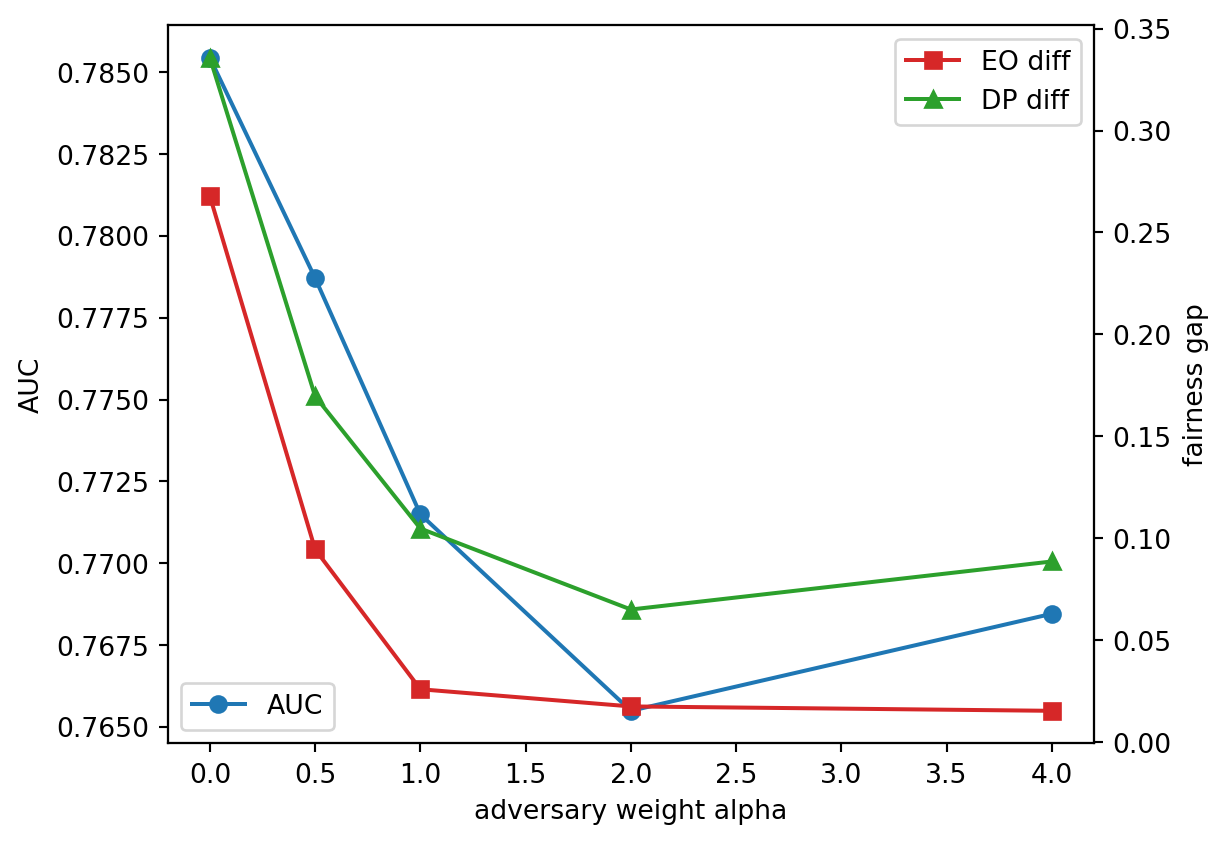
```{python}
#| label: adversarial-plot
#| fig-cap: "Accuracy vs equalized-odds trade-off as the adversarial weight alpha grows."
fig, ax1 = plt.subplots(figsize=(6.5, 4.5))
ax2 = ax1.twinx()
ax1.plot(trade["alpha"], trade["AUC"], "o-", color="tab:blue", label="AUC")
ax2.plot(trade["alpha"], trade["EO_diff"], "s-", color="tab:red", label="EO diff")
ax2.plot(trade["alpha"], trade["DP_diff"], "^-", color="tab:green", label="DP diff")
ax1.set_xlabel("adversary weight alpha")
ax1.set_ylabel("AUC")
ax2.set_ylabel("fairness gap")
ax1.legend(loc="lower left")
ax2.legend(loc="upper right")
fig.tight_layout()
plt.show()
```
The shape is the canonical Pareto curve: AUC falls as $\alpha$ grows, equalized-odds gap and demographic-parity gap both fall. Practitioners who need a defensible operating point pick $\alpha$ on this curve by either a policy rule ("we target EO diff $\le 0.05$") or by solving a regulatory cost/utility trade. There is no principled "right" $\alpha$; the curve is the answer, the single point is a business decision.
### Fair representations in one paragraph
Adversarial debiasing produces a fair classifier. A related line of work [@zemel2013learning; @madras2018learning] produces a fair representation $Z = \phi(X)$ that a downstream learner can use freely while retaining the fairness property. The trick is to train $\phi$ with three competing objectives: reconstruct $X$, predict $Y$ from $Z$, and be uninformative about $A$. The attraction for credit is that the representation can be shared across downstream tasks (origination, pricing, collections) without re-doing the debiasing. The cost is that all three downstream users must accept the same fairness target, which is rare when origination, pricing, and collections report to different risk committees.
---
## Putting the four treatments side by side
```{python}
#| label: all-methods-summary
from sklearn.metrics import accuracy_score

def summarize(name, p_pred, y_pred, y_true, a_true):
    return {
        "method":    name,
        "AUC":       roc_auc_score(y_true, p_pred),
        "accuracy":  accuracy_score(y_true, y_pred),
        "DP_diff":   demographic_parity_difference(y_true, y_pred, sensitive_features=a_true),
        "EO_diff":   equalized_odds_difference(y_true, y_pred, sensitive_features=a_true),
    }

p_adv_best = train_adversarial(alpha=2.0, epochs=200)
y_adv_best = (p_adv_best > 0.5).astype(int)

# for TO, we do not have a probability, but we can use the baseline probability for AUC
out = pd.DataFrame([
    summarize("baseline",                p_hat, y_hat, yte, Ate),
    summarize("reweighing",              p_rw,  y_rw,  yte, Ate),
    summarize("disparate-impact remover", p_dir, y_dir, yte, Ate),
    summarize("adversarial (alpha=2)",   p_adv_best, y_adv_best, yte, Ate),
    summarize("threshold optimizer (EO)", p_hat, y_hat_to, yte, Ate),
]).round(3)
print(out)
```
The ranking is what the theory predicts. The threshold optimizer minimizes the equalized-odds gap most aggressively but does not change statistical parity much. Reweighing nudges both gaps at zero accuracy cost. Disparate-impact remover cuts statistical parity hard but less on equalized odds. Adversarial debiasing trades AUC for both gaps; the amount of AUC given up is the tuning knob.
There is no uniformly dominant method. The choice is driven by which fairness target matches the legal argument you are going to make, and which accuracy degradation the portfolio can absorb.
---
## Scalability of the fairness pipeline
Reweighing and disparate-impact removal are single-pass operations: compute group-conditional CDFs, apply the transformation, refit. Both scale linearly with $n$ and are trivially distributable in Spark or Dask by broadcasting the per-group CDFs.
Post-processing with `ThresholdOptimizer` requires the full score vector and the protected attribute vector at prediction time. The ROC convex hulls can be constructed from per-group histograms of scores, which can be computed in Polars with a `group_by(A).agg` on quantile bins; for $n > 10^7$ this runs in under a minute on a laptop.
Adversarial debiasing is the expensive step. Training the classifier and adversary is GPU-friendly and scales like a standard deep net. The only fairness-specific scaling subtlety is that stochastic minibatches can have very few instances of a minority subgroup, which destabilizes the adversary. The standard remedy is stratified batching by $(A, Y)$ quadrants. With four quadrants and a minority share of 10 percent, a batch of 256 should oversample to at least 20 minority-group defaulters per batch.
Exponentiated-gradient reductions (`fairlearn.reductions.ExponentiatedGradient`) are linear in the number of inner ERM calls, typically 50 to 200 for reasonable fairness slack. On a credit-card dataset of a few million rows this is minutes with a fast base learner.
---
## Deployment and regulatory considerations
### Deployment notes
A deployed fair model has three moving parts: the trained probability predictor, the post-processing layer if any, and the audit logger that records $(X, A, S, \hat{Y}, Y)$ triples for later fairness review. Wrapping the predictor in FastAPI with an MLflow model URI is standard; the specific addition for a fair model is that the service must either have access to $A$ at inference time (needed for `ThresholdOptimizer.predict`) or must have a pre-processing pipeline that renders $A$ unnecessary at inference (reweighing and adversarial debiasing do).
If $A$ enters the decision surface at inference time, you have created disparate treatment unless the statute provides an affirmative authorization. ECOA provides no such authorization for race or national origin. The practical workaround, used by several banks under the CFPB's observation, is to validate a fair model offline but deploy a strictly $A$-blind policy, then monitor for disparate impact quarterly. This is the "fair training, blind inference" pattern, and it rules out `ThresholdOptimizer`-style post-processing by itself, since that rule is explicitly group-specific. Adversarial debiasing and reweighing survive the blind-inference constraint because both produce an inference function that does not use $A$.
### Regulatory mapping
Under SR 11-7 (Supervisory Guidance on Model Risk Management, Fed 2011), a fair-lending intervention is itself a model component and requires effective challenge, testing documentation, and ongoing monitoring. The reviewer will ask: why did you choose equalized odds over calibration? What does the impossibility theorem imply about the criterion you did not satisfy? What is the business-necessity basis for the remaining disparity?
Under ECOA and Regulation B, the fair-lending compliance team must produce a record showing the four-fifths computation, a statistical significance test, the choice of benchmark, the business-necessity argument, and the consideration of less discriminatory alternatives (LDAs). The LDA requirement is the one that most often defeats naive fair-lending defenses in U.S. credit supervision: the regulator asks whether any LDA was considered that would have achieved similar business outcomes with smaller disparity, and if the answer is "we didn't look," the file is incomplete.
Under the EU AI Act, Article 10 requires that high-risk systems be trained on data sets that are subject to "appropriate data governance and management practices," including examination in view of possible biases that may affect fundamental rights. Article 15 requires accuracy, robustness, and cybersecurity. Neither mandates a specific fairness definition. Both effectively require that the lender be able to state, document, and justify a choice. The chapter's taxonomy is the menu from which that choice is made.
Under GDPR Article 22, a decision "based solely on automated processing" that has legal or similarly significant effects requires human review or an exception (contract, consent, or authorized law). Most lenders claim the "necessary for a contract" exception under Article 22(2)(a), but the decision must still be accompanied by "meaningful information about the logic involved," which Recital 71 links to fair processing. An adversarially-debiased or reweighted model satisfies this only if the team can explain why that intervention was preferred over the alternatives: calibration, threshold adjustment, fair representations.
### Model documentation
Whatever method is adopted, the fairness-documentation artifact in a model risk file contains four things: a statement of the chosen fairness criterion and the legal rationale; a quantified demonstration of the criterion on training and holdout; a quantified statement of what other criteria do under the chosen intervention, including the calibration criterion; and a monitoring plan that re-estimates all these numbers on a recurring cadence. The numerical code in this chapter produces all four.
---
## Vietnam and emerging markets
### Market context
Vietnam has no direct equivalent of the Equal Credit Opportunity Act. The general anti-discrimination framework sits across several statutes. The Law on Gender Equality, No. 73/2006/QH11 [@vn_law_gender_equality_2006], prohibits discrimination on the basis of sex in economic activity and state management. The Law on Persons with Disabilities, No. 51/2010/QH12 [@vn_law_disabilities_2010], requires the state and credit institutions to support access to finance for persons with disabilities, without specifying a scoring rule. The 2013 Constitution prohibits discrimination on the basis of ethnicity, religion, sex, social origin, belief, and social status, but does not create a private cause of action against a lender. There is no Vietnamese analog of Regulation B, no four-fifths rule, no CFPB-style circular, and no reported case law in which a denied applicant successfully sued a lender for disparate impact. Fairness in Vietnamese lending is therefore ethical, reputational, and increasingly tied to ESG disclosure rather than codified in consumer protection.
The social context that fairness analysis must reflect is still sharp. Vietnam recognizes 54 ethnic groups, with the Kinh majority accounting for roughly 85 percent of the population and 53 other groups concentrated in the Northern mountains, the Central Highlands, and the Mekong Delta margins. Rural and urban gaps in bureau coverage are material. The CIC covers a substantially smaller fraction of adults in rural provinces than in Hanoi and Ho Chi Minh City [@cic_vietnam2023], and thin-file rural borrowers are routinely declined by scoring models that were trained on urban samples. Gender patterns in self-employment, informal work, and household headship also produce measurable score gaps, though these gaps do not map cleanly to the US or EU protected-class taxonomy.
### Application considerations
A fairness audit in Vietnam is not a test against a statutory rule; it is a test against an internal policy that the lender writes. Three audits are defensible in the current market. The first is a group-level disparity report on gender, computed in the same way as a US four-fifths report, run quarterly, and disclosed to the risk committee. The second is a rural-versus-urban disparity report, computed by province code or by the CIC-derived residency flag. The third is an ethnic-majority-versus-minority report, which is harder because most credit institutions do not store ethnicity as a feature. In that case, the audit uses geography, language of application, and surname heuristics as imperfect proxies, and reports the estimated bound rather than a point estimate.
The fairness mathematics in this chapter travel unchanged. Demographic parity, equalized odds, calibration, and the impossibility theorem of @chouldechova2017fair and @kleinberg2017inherent depend on base rates and score distributions, not on statute. What changes is the enforcement model. In the US, a four-fifths violation triggers a regulator referral. In Vietnam, it triggers a conversation with the parent group's compliance team, a line in the annual sustainability report, and in some cases a discussion with the IFC or a development finance investor.
### Rationalization
The case for fairness work in Vietnam rests on three pillars. The first is ESG disclosure. Larger Vietnamese banks are moving toward voluntary adoption of the IFC Performance Standards and SBV Circular 17/2022/TT-NHNN on environmental risk management in credit-granting activity. A fairness audit is one of the few quantitative artifacts that can go into an ESG report without translation. The second is parent-group policy. Foreign-owned finance companies and joint-venture banks typically inherit a group fairness policy from Seoul, Tokyo, Paris, or Frankfurt. The third is preparatory work for the rule that market participants expect. An SBV circular on algorithmic lending has been under discussion since 2023, and firms that have a running fairness pipeline will adapt to it faster than firms that do not.
### Practical notes
Build the audit pipeline before the rule arrives. Use `fairlearn` for the US-style metrics, Run the audit by gender, by urban-rural, and by region. Treat ethnicity as a proxy exercise, not a direct measurement. Document the fairness definition you chose and the definition you sacrificed, using the impossibility theorem as the justification, because the parent group or the ESG auditor will ask. Do not attempt disparate-impact litigation defense in Vietnam, because the cause of action does not yet exist; instead, document the business necessity argument for any feature that produces large group disparity, because that documentation is what the SBV examiner is most likely to read.
## Takeaways
- Fairness in credit decomposes into three incompatible families: distribution parity (DP and conditional DP), error-rate parity (EO, predictive equality, equal opportunity), and outcome parity (calibration, PPV). The choice is legal first and technical second.
- The impossibility theorems of @chouldechova2017fair and @kleinberg2017inherent show that when base rates differ, you can satisfy at most two of {calibration, balance for positives, balance for negatives}. Any "fair" model is therefore a choice of which criterion to sacrifice.
- Each of the three intervention families does something different: pre-processing reweights or repairs features and leaves the learner alone; in-processing changes the objective through adversarial or Lagrangian terms; post-processing adjusts the decision rule after training.
- Post-processing [@hardt2016equality] is a small linear program that chooses group-specific randomized thresholds on the group-wise ROC convex hulls. It is fast and exactly hits equalized odds but breaks calibration.
- Adversarial debiasing sweeps out a Pareto curve between accuracy and fairness; the operating point is a business decision, not an optimization output.
- Under ECOA, a deployed model that uses $A$ at inference time creates disparate treatment. Fair training plus blind inference is the default U.S. pattern.
## Further reading
- @hardt2016equality for the original equalized-odds post-processing construction.
- @chouldechova2017fair and @kleinberg2017inherent for the two complementary statements of the impossibility result.
- @kusner2017counterfactual and @kilbertus2017avoiding for the causal branch of fairness.
- @dwork2012fairness for the Lipschitz "fairness through awareness" frame.
- @agarwal2018reductions for the reductions approach and `ExponentiatedGradient`.
- @zhang2018mitigating for adversarial debiasing.
- @kamiran2012data for reweighing and @feldman2015certifying for disparate-impact remediation.
- @pleiss2017fairness for the calibration versus error-rate tension.
- @barocas2016big and @hurley2016credit for the legal-framework background.
- @bartlett2022consumer23 and @fuster2022predictably for empirical evidence of disparities in consumer-credit machine-learning pipelines.
- @corbett2017algorithmic for the cost-of-fairness analysis.
- @mehrabi2021survey for a survey of the broader literature.