---
execute:
echo: true
eval: true
bibliography: [../references.bib, ../refs/ch-06.bib]
---
# Discriminant Analysis and the Altman Z-Score {#sec-ch06}
::: {.callout-note appearance="simple" icon="false"}
**Scope: corporate.** Altman MDA, Z'/Z'', Ohlson, Shumway, and Campbell-Hilscher-Szilagyi on the UCI 572 Taiwanese Bankruptcy panel. Consumer applicability is discussed only in @sec-ch06-limitations.
:::
## Overview {.unnumbered}
Linear discriminant analysis was the first statistical tool a bank analyst could hand to a credit committee with a coefficient table and a decision rule. It still is, in many corporate risk groups, because regulators, auditors, and working capital officers can read it. @altman1968zscore turned Fisher's 1936 idea into a working bankruptcy filter by fitting a five-ratio discriminant function on a matched sample of 66 manufacturers. More than five decades later, the Z-score survives as a monitoring metric, a covenant trigger, and a classroom staple. The method is no longer state of the art for out-of-sample accuracy, but it is a lower bound on interpretability and a useful calibration against fancier models.
This chapter rebuilds that machinery end to end. The formal part derives Fisher's criterion from the between-to-within variance ratio, proves its equivalence to the Bayes rule under Gaussian equal-covariance class-conditionals, and extends to quadratic discriminant analysis (@sec-ch06-qda) when covariances differ. The empirical part replays the Altman MDA on the @liang2016financial Taiwanese Bankruptcy Prediction panel (UCI 572: 6,819 firm-years, 220 bankruptcies), then steps through the Z', Z'', and ZETA extensions. The benchmark part puts LDA head to head with logistic regression, Ohlson's logit, Shumway's hazard model, and the Campbell-Hilscher-Szilagyi distance measure (@sec-ch06-chs), and documents where LDA still wins and where it loses badly.
A pragmatic warning first. LDA on raw consumer-credit features, with their mixture of one-hot dummies and skewed amounts, is almost always dominated by a penalized logit or a gradient-boosted tree on the same design matrix. The reason is not that LDA is wrong in principle. It is that its generative Gaussian assumption is wrong in that particular setting. Where features really are close to jointly Gaussian, LDA remains statistically efficient [@efron1975efficiency]. The chapter gives the conditions and shows them in code.
An emerging-market framing sits underneath the whole chapter. In Vietnam and peer economies, corporate books are dominated by thin-file private SMEs whose audited financials arrive late, if at all. Household lending is pulled around by the Tet holiday liquidity cycle, informal-income cash flows, and macro volatility. An LDA or Z''-style model is often the only thing a credit committee in Ho Chi Minh City or Hanoi will approve for middle-market corporate scoring, because the coefficient table is auditable and the sample sizes do not support heavier machinery. The emerging-market section at the end of the chapter returns to this with the CIC bureau, SBV Circular 11/2021, and practical notes on fitting Z'' to Vietnamese manufacturers.
### Notation {.unnumbered}
Let $X \in \mathbb{R}^p$ be the feature vector and $Y \in \{0, 1\}$ the default indicator, with 1 coding default. Write $\pi_k = \Pr(Y = k)$, $\mu_k = \mathbb{E}[X \mid Y = k]$, and $\Sigma_k = \operatorname{Var}(X \mid Y = k)$. When the common-covariance assumption holds, $\Sigma_0 = \Sigma_1 = \Sigma$. Sample estimates are hatted. The within-class scatter is $S_W$ and the between-class scatter is $S_B$. $\Phi$ is the standard normal CDF. For firm-level work, $X_1, \dots, X_5$ name the Altman ratios in the order he wrote them.
## Motivation {.unnumbered}
Banks run two kinds of default models at a minimum: one for corporates and large SMEs, scored on financial statements, and one for consumer accounts, scored on application plus bureau data. @beaver1966financial showed that individual accounting ratios discriminate between bankrupt and healthy firms one to five years out, but he scored one ratio at a time. The weakness is obvious: ratios are correlated, the information is redundant, and a single-ratio cutoff throws away the multivariate signal.
@altman1968zscore fixed this with Fisher's multiple discriminant analysis (MDA). He picked five ratios out of an initial list of 22, fit a linear discriminant on a paired sample of 33 bankrupt and 33 non-bankrupt manufacturers over 1946 to 1965, and published a scoring function that bank analysts could compute by hand. The published function, his decision zones, and his out-of-sample hit rate (95 percent on the original sample, about 80 percent at two-year horizons on holdout) made the Z-score the reference point every later bankruptcy model had to beat.
Three things changed after 1980. @ohlson1980financial showed that a logit on nine variables beat the Z-score on a bigger sample, because binary outcomes with mixed-type predictors fit the logit log-likelihood better than the Gaussian likelihood behind LDA. @shumway2001forecasting reframed bankruptcy as a time-to-event process and built a multi-period hazard model, which avoids the selection bias baked into static matched samples. The derivation, pooled-logit equivalence, and its place in the lineage appear in @sec-ch06-empirical of this chapter; the full implementation (long-table construction, time-varying covariates, term-structure recovery, and the current state of the art) is developed in @sec-ch09-shumway, with the connection to distance-to-default covered in @sec-ch08-empirical. @campbell2008search combined accounting and market-based inputs, including volatility and equity returns, and improved out-of-sample ranking further. The sequence from Altman through Campbell is a textbook instance of the same phenomenon, climbing a ladder of statistical sophistication, while the underlying economics stay close to "leverage, profitability, liquidity, size."
This chapter keeps the whole ladder in one place. @sec-ch06 derives LDA from scratch. @sec-ch06-altman reconstructs Altman's Z. Sections [-@sec-ch06-extensions] and [-@sec-ch06-empirical] step through its extensions and its empirical competitors. @sec-ch06-limitations returns to the original question: when does the linear-Gaussian generative model win against the discriminative logit?
## Formal setup {.unnumbered}
A credit classifier produces a score $s(x) \in \mathbb{R}$ for each applicant vector $x \in \mathbb{R}^p$. A decision rule declares default when $s(x) > t$ for some threshold $t$. Quality of the score is measured by a ranking metric (AUC, KS) and by calibration to the observed default rate in bins.
Three ingredients separate LDA from its alternatives.
1. **A generative assumption on the class-conditional distribution**. LDA posits $X \mid Y = k \sim \mathcal{N}(\mu_k, \Sigma)$ with shared covariance. QDA relaxes to $\Sigma_k$. Naive Bayes factors the density across features. Logistic regression makes no density assumption at all and models $\Pr(Y \mid X)$ directly.
2. **An estimation procedure**. LDA uses the sample class means and pooled covariance, which are the maximum-likelihood estimators under the Gaussian assumption. Logit uses maximum-likelihood estimation of the conditional density. Both converge at the standard parametric rate $n^{-1/2}$ to their respective targets.
3. **A decision function**. LDA's is $\hat\Sigma^{-1}(\hat\mu_1 - \hat\mu_0)$. Logit's is the MLE of the log-odds coefficient. When the LDA assumptions hold, both targets coincide and the question is efficiency. When they fail, LDA's estimand is no longer the Bayes rule and logit wins by consistency.
The chapter walks through these three ingredients in order, first for the two-class case that matches corporate bankruptcy, then for the multi-class case that matches rating-grade assignment, then back to binary with the full credit-scoring machinery around it.
## Linear discriminant analysis {#sec-ch06-discriminant}
### Fisher's criterion
@fisher1936use asked for a linear projection $w^\top X$ of the feature vector that separates the two classes as well as possible. Measure separation by the ratio of between-class to within-class variance along the projected axis. If $\mu_0, \mu_1 \in \mathbb{R}^p$ are the class means and $\Sigma_0, \Sigma_1$ are the class covariances, the projected between-class squared distance is $\left(w^\top(\mu_1 - \mu_0)\right)^2$, and the projected within-class variance is $w^\top(\Sigma_0 + \Sigma_1) w$ up to class weights. Fisher's criterion is
$$
J(w) = \frac{\bigl(w^\top(\mu_1 - \mu_0)\bigr)^2}{w^\top \Sigma_W w} = \frac{w^\top S_B w}{w^\top S_W w},
$$ {#eq-fisher-ratio}
where $S_B = (\mu_1 - \mu_0)(\mu_1 - \mu_0)^\top$ is the rank-one between-class scatter and $S_W = \pi_0 \Sigma_0 + \pi_1 \Sigma_1$ is the within-class scatter. The objective is scale-invariant in $w$, so fix $w^\top S_W w = 1$. The Lagrangian is
$$
\mathcal{L}(w, \lambda) = w^\top S_B w - \lambda\bigl(w^\top S_W w - 1\bigr).
$$ {#eq-fisher-lagrangian}
Stationarity $\partial\mathcal{L}/\partial w = 0$ gives the generalized eigenvalue problem
$$
S_B w = \lambda S_W w.
$$ {#eq-fisher-gep}
When $S_W$ is positive definite, left-multiply by $S_W^{-1}$ to get the standard eigenvalue problem $S_W^{-1} S_B w = \lambda w$. Because $S_B$ has rank 1 in the two-class case, there is exactly one non-zero eigenvalue, and the corresponding eigenvector is proportional to $S_W^{-1}(\mu_1 - \mu_0)$. The maximum value of the criterion equals that eigenvalue and is the squared Mahalanobis distance between the class means [@mahalanobis1936generalized]:
$$
\max_{w \ne 0} J(w) = (\mu_1 - \mu_0)^\top \Sigma^{-1} (\mu_1 - \mu_0) = \Delta^2.
$$ {#eq-mahalanobis}
In the $K > 2$ class case, $S_B$ has rank up to $K - 1$, and the discriminant projection has $K - 1$ directions. This is the "multiple" in MDA [@rao1948utilization].
The geometric content deserves a second pass. Write the within-class scatter as a symmetric positive-definite matrix and factor it as $S_W = L L^\top$ via Cholesky. Substitute $u = L^\top w$. The criterion becomes
$$
J(w) = \frac{u^\top (L^{-1} S_B L^{-\top}) u}{u^\top u}.
$$ {#eq-fisher-whitened}
The Lagrangian now has the structure of an ordinary Rayleigh quotient. The optimal $u^\star$ is the top eigenvector of the symmetric matrix $L^{-1} S_B L^{-\top}$, and we recover $w^\star = L^{-\top} u^\star$. Equivalently, Fisher's projection is the linear direction that would be maximally separating in a whitened coordinate system where the within-class scatter is isotropic. This is also how @bickel2004some interpret LDA's failure in high dimensions: the whitening step breaks when $L$ is near-singular, and the finite-sample direction diverges from the true Bayes direction even with moderate dimension.
### Equivalence with the decorrelated signal-to-noise direction
Start from a different angle. Suppose $X \mid Y = k \sim \mathcal{N}(\mu_k, \Sigma)$. Let $Z = \Sigma^{-1/2}(X - \bar\mu)$ where $\bar\mu = (\mu_0 + \mu_1)/2$. Under the change of variables, $Z \mid Y = k \sim \mathcal{N}\bigl(\tfrac{1}{2}(-1)^{1-k} \Sigma^{-1/2}(\mu_1-\mu_0), I\bigr)$. The two class distributions are now unit-covariance Gaussians symmetric about the origin, separated along the direction $d = \Sigma^{-1/2}(\mu_1 - \mu_0)$. The Bayes rule reduces to thresholding the projection $d^\top Z$, and in the original coordinate system that projection is $(\Sigma^{-1/2})^\top d \cdot (X - \bar\mu) = \Sigma^{-1}(\mu_1-\mu_0) \cdot (X - \bar\mu)$. Same answer, different derivation, same coefficient $\beta = \Sigma^{-1}(\mu_1 - \mu_0)$.
The Mahalanobis distance @eq-mahalanobis controls the discriminability. When $\Delta$ is small, no linear rule separates well; any competing non-linear rule that does better must be exploiting non-Gaussian, not geometry. When $\Delta$ is large, almost any sensible rule works, and the optimization details stop mattering. @anderson1951classification formalized this and gave the asymptotic error rate for Fisher's rule as $\Phi(-\Delta/2)$ when the priors are equal, which is the quantity most later empirical papers use as a benchmark.
### Sample-size corrections and plug-in bias
In practice, $\Sigma$ is unknown and we plug in a sample estimate. The unbiased within-class covariance is
$$
\hat\Sigma = \frac{1}{n-2}\left[\sum_{i: y_i=0} (x_i - \hat\mu_0)(x_i - \hat\mu_0)^\top
+ \sum_{i: y_i=1} (x_i - \hat\mu_1)(x_i - \hat\mu_1)^\top\right].
$$ {#eq-pooled-cov}
Plugging $\hat\Sigma$ and $\hat\mu_k$ into the Bayes rule produces a linear classifier whose error exceeds the Bayes error by an $O(p/n)$ term [@anderson1951classification]. @bickel2004some show that as $p/n \to \gamma > 0$, the classifier loses all discriminative power unless $\Sigma$ has structure (sparsity, block-diagonality, a factor model). In the $p \ll n$ regime relevant to Altman's 5-variable model on 66 firms, the plug-in correction is small. In the consumer-credit regime with 50 to 200 dummies on a few thousand applicants, it is not.
A partial fix is regularized discriminant analysis [@friedman1989regularized], which shrinks $\hat\Sigma_k$ toward a pooled covariance and a diagonal target to trade bias against variance. The full derivation, the hyperparameter grid, and a runnable comparison against LDA and QDA appear in @sec-ch06-rda.
### Bayes decision under Gaussian equal-covariance
Now change view. Suppose the class-conditional densities are multivariate Gaussian with a common covariance:
$$
X \mid Y = k \sim \mathcal{N}(\mu_k, \Sigma), \qquad k = 0, 1.
$$ {#eq-gaussian-classes}
The posterior log-odds reduce to a linear discriminant. Write the log-posterior ratio:
$$
\begin{aligned}
\log\frac{\Pr(Y=1\mid X)}{\Pr(Y=0\mid X)}
={}& \log\frac{\pi_1}{\pi_0} - \tfrac12 (X-\mu_1)^\top \Sigma^{-1}(X-\mu_1) \\
& + \tfrac12 (X-\mu_0)^\top \Sigma^{-1}(X-\mu_0).
\end{aligned}
$$ {#eq-posterior-logodds}
The quadratic terms in $X$ cancel under equal covariance, leaving
$$
\begin{aligned}
\log\frac{\Pr(Y=1\mid X)}{\Pr(Y=0\mid X)}
={}& X^\top \Sigma^{-1}(\mu_1-\mu_0) \\
& - \tfrac12(\mu_1+\mu_0)^\top \Sigma^{-1}(\mu_1-\mu_0) + \log\frac{\pi_1}{\pi_0}.
\end{aligned}
$$ {#eq-lda-logit}
The Bayes-optimal classifier thresholds this linear function of $X$. The coefficient vector $\Sigma^{-1}(\mu_1 - \mu_0)$ is exactly the Fisher direction @eq-fisher-gep up to scaling, so the two derivations coincide. The intercept differs only by the prior adjustment $\log(\pi_1/\pi_0)$ and the midpoint term, which Fisher's variance-ratio criterion does not fix because it is scale and location invariant.
Three consequences matter in practice. First, LDA is linear in $X$, so the decision boundary is a hyperplane. Second, its coefficients are interpretable in the same way OLS coefficients are, because they come from inverting a single covariance matrix. Third, the estimated probability
$$
\Pr(Y=1 \mid X) = \sigma\!\left(X^\top \beta + \beta_0\right), \qquad \beta = \Sigma^{-1}(\mu_1 - \mu_0),
$$ {#eq-lda-sigmoid}
is correctly calibrated when the Gaussian assumption holds. When it does not hold, the resulting probabilities are often miscalibrated even if the ranking remains good. This matters for credit scorecards because regulators expect the probability of default, not only its rank.
### Quadratic discriminant analysis {#sec-ch06-qda}
Drop the equal-covariance assumption. Let $X \mid Y = k \sim \mathcal{N}(\mu_k, \Sigma_k)$. The same algebra yields
$$
\log\frac{\Pr(Y=1\mid X)}{\Pr(Y=0\mid X)} = -\tfrac12 X^\top(\Sigma_1^{-1} - \Sigma_0^{-1}) X + X^\top(\Sigma_1^{-1}\mu_1 - \Sigma_0^{-1}\mu_0) + C,
$$ {#eq-qda-logit}
where $C$ collects the scalar intercept with $\log(\pi_1/\pi_0)$, $\log|\Sigma_k|$ terms, and quadratic terms in the class means. The decision surface is now a quadric, not a hyperplane. QDA has $p(p+1)$ parameters in the covariance blocks versus $p(p+1)/2$ for LDA, so it overfits quickly when $p$ grows relative to $n$ [@friedman1989regularized].
For credit work, QDA is the natural upgrade when defaulters show a different covariance structure from survivors. That is common in practice: distressed firms have fatter tails and more correlated deterioration across ratios. Whether QDA actually beats LDA depends on whether you have enough defaulters to estimate $\Sigma_1$ well. When the defaulter sample is too thin to support separate covariances but LDA's equal-covariance constraint is visibly wrong, the regularized path in @sec-ch06-rda is the practical middle ground.
### Regularized discriminant analysis {#sec-ch06-rda}
@friedman1989regularized proposed a two-parameter shrinkage that interpolates between LDA (@sec-ch06-discriminant) and QDA (@sec-ch06-qda) and then shrinks each covariance toward its diagonal:
$$
\hat\Sigma_k(\alpha, \gamma) = (1 - \gamma)\left[(1 - \alpha)\hat\Sigma_k + \alpha \hat\Sigma_{\text{pool}}\right]
+ \gamma \operatorname{diag}\!\left(\hat\Sigma_k\right).
$$ {#eq-rda-shrink}
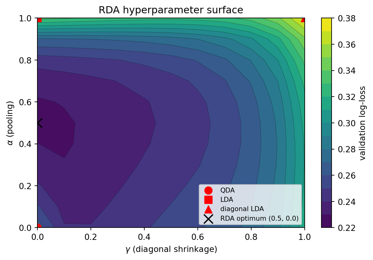
The two hyperparameters index a rectangle of models. At $\alpha = 1, \gamma = 0$ the pooled covariance recovers LDA. At $\alpha = 0, \gamma = 0$ the class-specific covariances recover QDA. At $\alpha = 1, \gamma = 1$ the pooled diagonal reproduces diagonal LDA, which under Gaussian marginals is Gaussian naive Bayes. The interior of the rectangle covers the intermediate regularization paths.
The first parameter $\alpha$ controls covariance pooling. Pure QDA uses $\hat\Sigma_k$ estimated on the $n_k$ observations of class $k$, which has $p(p+1)/2$ free parameters per class. When the rarer class carries a few dozen observations (the Altman 33 defaulters, a stressed emerging-market corporate book, a tail-event sample), $\hat\Sigma_1$ is noisy and QDA's quadratic decision surface follows the noise. Shrinking toward $\hat\Sigma_{\text{pool}}$ borrows strength from the larger class at the cost of a small bias if the covariances truly differ.
The second parameter $\gamma$ controls diagonal shrinkage. The off-diagonal entries of $\hat\Sigma_k$ are noisier than the diagonal in high dimension [@bickel2004some], and setting $\gamma > 0$ throws away the noisiest entries. The limit $\gamma = 1$ is diagonal LDA, which assumes feature independence within a class; the limit $\gamma = 0$ keeps the full sample covariance.
For small samples with modest $p$, a cross-validated RDA typically outperforms both pure LDA and pure QDA. It is a good default when the modeler is uncertain about the covariance structure, because the optimal $(\alpha, \gamma)$ tells the modeler which assumption was closer to the data without a separate hypothesis test.
```{python}
#| fig-cap: "Validation log-loss surface for RDA on an eight-feature heteroskedastic sample with a thin minority class (n=60 defaulters, Altman-scale). Red markers locate the pure-LDA, pure-QDA, and diagonal-LDA corners; the black cross marks the cross-validated optimum, which sits in the interior."
import numpy as np
import matplotlib.pyplot as plt
from sklearn.discriminant_analysis import (
    LinearDiscriminantAnalysis,
    QuadraticDiscriminantAnalysis,
)
from sklearn.metrics import log_loss


def rda_covariances(X, y, alpha, gamma):
    classes = np.unique(y)
    covs_class, priors, means = {}, {}, {}
    Xc_all = []
    for c in classes:
        Xc = X[y == c]
        means[c] = Xc.mean(0)
        priors[c] = len(Xc) / len(X)
        covs_class[c] = np.cov(Xc, rowvar=False, bias=False)
        Xc_all.append(Xc - means[c])
    Sigma_pool = np.cov(np.vstack(Xc_all), rowvar=False, bias=False)
    reg_covs = {}
    for c in classes:
        S = (1 - alpha) * covs_class[c] + alpha * Sigma_pool
        S = (1 - gamma) * S + gamma * np.diag(np.diag(S))
        reg_covs[c] = S
    return means, priors, reg_covs


def rda_predict_proba(X_tr, y_tr, X_te, alpha, gamma):
    means, priors, covs = rda_covariances(X_tr, y_tr, alpha, gamma)
    logs = []
    for c in sorted(means):
        S = covs[c]
        sign, logdet = np.linalg.slogdet(S)
        diff = X_te - means[c]
        quad = np.einsum("ni,ij,nj->n", diff, np.linalg.inv(S), diff)
        logs.append(np.log(priors[c]) - 0.5 * logdet - 0.5 * quad)
    logs = np.column_stack(logs)
    logs -= logs.max(1, keepdims=True)
    P = np.exp(logs)
    return P / P.sum(1, keepdims=True)


# Eight financial-ratio features, Altman-scale minority class.
rng_h = np.random.default_rng(3)
p_feat, n0h, n1h = 8, 400, 60
mu0 = np.zeros(p_feat)
mu1 = np.ones(p_feat) * 0.6
Sigma0 = 0.3 * np.ones((p_feat, p_feat)) + 0.7 * np.eye(p_feat)
A_rand = rng_h.standard_normal((p_feat, p_feat))
Sigma1 = A_rand @ A_rand.T / p_feat + 0.5 * np.eye(p_feat)
X0h = rng_h.multivariate_normal(mu0, Sigma0, n0h)
X1h = rng_h.multivariate_normal(mu1, Sigma1, n1h)
Xh_rda = np.vstack([X0h, X1h])
yh_rda = np.hstack([np.zeros(n0h), np.ones(n1h)])
perm = rng_h.permutation(len(yh_rda))
split = int(0.7 * len(yh_rda))
tr, te = perm[:split], perm[split:]

alphas = np.linspace(0.0, 1.0, 11)
gammas = np.linspace(0.0, 1.0, 11)
loss = np.zeros((len(alphas), len(gammas)))
for i, a in enumerate(alphas):
    for j, g in enumerate(gammas):
        P = rda_predict_proba(Xh_rda[tr], yh_rda[tr], Xh_rda[te], a, g)
        loss[i, j] = log_loss(yh_rda[te], P[:, 1], labels=[0, 1])

i_star, j_star = np.unravel_index(np.argmin(loss), loss.shape)
a_star, g_star = alphas[i_star], gammas[j_star]

fig, ax = plt.subplots(figsize=(6.5, 4.5))
cs = ax.contourf(gammas, alphas, loss, levels=15, cmap="viridis")
ax.contour(gammas, alphas, loss, levels=15, colors="k", linewidths=0.4, alpha=0.4)
plt.colorbar(cs, ax=ax, label="validation log-loss")
ax.scatter([0.0], [0.0], color="red", s=80, label="QDA")
ax.scatter([0.0], [1.0], color="red", s=80, marker="s", label="LDA")
ax.scatter([1.0], [1.0], color="red", s=80, marker="^", label="diagonal LDA")
ax.scatter([g_star], [a_star], color="black", s=120, marker="x",
           label=f"RDA optimum ({a_star:.1f}, {g_star:.1f})")
ax.set_xlabel(r"$\gamma$ (diagonal shrinkage)")
ax.set_ylabel(r"$\alpha$ (pooling)")
ax.set_title("RDA hyperparameter surface")
ax.legend(loc="lower right", fontsize=8)
fig.tight_layout()
plt.show()

lda_ll = log_loss(yh_rda[te],
                  LinearDiscriminantAnalysis().fit(Xh_rda[tr], yh_rda[tr])
                      .predict_proba(Xh_rda[te])[:, 1], labels=[0, 1])
qda_ll = log_loss(yh_rda[te],
                  QuadraticDiscriminantAnalysis().fit(Xh_rda[tr], yh_rda[tr])
                      .predict_proba(Xh_rda[te])[:, 1], labels=[0, 1])
print(f"LDA  log-loss: {lda_ll:.3f}")
print(f"QDA  log-loss: {qda_ll:.3f}")
print(f"RDA  log-loss: {loss[i_star, j_star]:.3f} at (alpha, gamma) = ({a_star:.2f}, {g_star:.2f})")
```
RDA finds an interior $(\alpha, \gamma)$ that beats both corners. On a Gaussian-equal-covariance sample, the optimum would collapse to the LDA corner; on a sample with distinct covariances and a small minority class the optimum is typically in the interior. For credit work, this matters most in two settings: corporate distress scoring with a dozen or two defaulters per year, and consumer-credit segments like fraud-adjacent cohorts where the rarer class is both thin and heteroskedastic. Either way the cost is one cross-validation grid over a $11 \times 11$ rectangle, which is negligible next to the downstream calibration and monitoring pipeline.
A caveat: RDA inherits LDA's generative Gaussian assumption. It handles covariance misspecification but not the failure modes documented in @sec-ch06-limitations (heavy categoricals, skewed amounts, rare-event bias). On a mixed-type consumer design matrix, a well-tuned regularized logit remains the better default; RDA is the right tool when the predictors are continuous financial ratios and the sample is too thin for unconstrained QDA.
### From-scratch Fisher LDA
The following block implements LDA from the generalized eigenvalue system @eq-fisher-gep and compares it to `sklearn`. It also verifies the closed-form equivalence $w \propto S_W^{-1}(\mu_1 - \mu_0)$.
```{python}
import numpy as np
import pandas as pd
import matplotlib.pyplot as plt
import sys

sys.path.insert(0, '../code')
from creditutils import load_german_credit, ks_statistic, train_valid_test_split

np.random.seed(7)
rng = np.random.default_rng(7)

# Two Gaussian classes sharing a covariance.
mu0 = np.array([-1.0, -0.5])
mu1 = np.array([1.2, 0.8])
Sigma = np.array([[1.0, 0.3], [0.3, 1.4]])
L = np.linalg.cholesky(Sigma)

n0, n1 = 400, 400
X0 = mu0 + rng.standard_normal((n0, 2)) @ L.T
X1 = mu1 + rng.standard_normal((n1, 2)) @ L.T
X = np.vstack([X0, X1])
y = np.hstack([np.zeros(n0), np.ones(n1)])


def fisher_lda(X, y):
    """Two-class Fisher LDA via the generalized eigenvalue problem."""
    classes = np.unique(y)
    mu = {c: X[y == c].mean(0) for c in classes}
    Sw = np.zeros((X.shape[1], X.shape[1]))
    for c in classes:
        Xc = X[y == c] - mu[c]
        Sw += Xc.T @ Xc
    diff = (mu[1] - mu[0]).reshape(-1, 1)
    Sb = diff @ diff.T
    # Solve S_W^{-1} S_B w = lambda w.
    A = np.linalg.solve(Sw, Sb)
    vals, vecs = np.linalg.eig(A)
    idx = int(np.argmax(vals.real))
    w = vecs[:, idx].real
    w = w / np.linalg.norm(w)
    # Closed form for the two-class case.
    w_closed = np.linalg.solve(Sw, (mu[1] - mu[0]))
    w_closed = w_closed / np.linalg.norm(w_closed)
    mid = 0.5 * (mu[0] + mu[1])
    threshold = float(w_closed @ mid)
    return w, w_closed, threshold, Sw, mu


w_eig, w_closed, thr, Sw, mu = fisher_lda(X, y)
print("Eigen direction :", np.round(w_eig, 4))
print("Closed direction:", np.round(w_closed, 4))
print("Cosine alignment:", float(abs(w_eig @ w_closed)))
```
The two directions agree exactly up to sign because the rank-one $S_B$ forces the sole non-trivial eigenvector to lie along $S_W^{-1}(\mu_1 - \mu_0)$. Now verify against `sklearn`:
```{python}
from sklearn.discriminant_analysis import LinearDiscriminantAnalysis

lda = LinearDiscriminantAnalysis(store_covariance=True).fit(X, y)
coef_sklearn = lda.coef_.ravel()
coef_ours = np.linalg.solve(Sw / (len(y) - 2), (mu[1] - mu[0]))
print("sklearn coef     :", np.round(coef_sklearn, 4))
print("from-scratch coef:", np.round(coef_ours, 4))
print("ratio (should be const):", np.round(coef_sklearn / coef_ours, 4))

# Same accuracy.
proj = X @ w_closed
yhat_scratch = (proj > thr).astype(int)
print("from-scratch accuracy:", float((yhat_scratch == y).mean()))
print("sklearn accuracy     :", float(lda.score(X, y)))
```
Both implementations return the same linear decision rule up to a positive scaling and produce identical predictions on this sample.
### Decision boundary plot
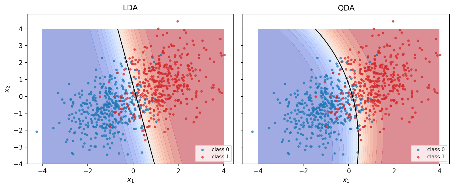
The LDA boundary is the set where @eq-lda-logit equals zero. For the shared-covariance case it is a straight line. QDA (@sec-ch06-qda) adds the quadratic terms in @eq-qda-logit, producing a conic boundary.
```{python}
#| fig-cap: "Decision boundaries for LDA and QDA on the shared-covariance sample. LDA recovers the Bayes linear rule; QDA adds a spurious curvature because it overfits the sample covariance."
from sklearn.discriminant_analysis import QuadraticDiscriminantAnalysis

xx, yy = np.meshgrid(np.linspace(-4, 4, 300), np.linspace(-4, 4, 300))
grid = np.c_[xx.ravel(), yy.ravel()]

fig, axes = plt.subplots(1, 2, figsize=(10, 4.2), sharey=True)
for ax, model, name in [(axes[0], lda, "LDA"),
                         (axes[1], QuadraticDiscriminantAnalysis().fit(X, y), "QDA")]:
    Z = model.predict_proba(grid)[:, 1].reshape(xx.shape)
    ax.contourf(xx, yy, Z, levels=20, cmap="coolwarm", alpha=0.5)
    ax.contour(xx, yy, Z, levels=[0.5], colors="k", linewidths=1.2)
    ax.scatter(X0[:, 0], X0[:, 1], s=8, color="#1f77b4", alpha=0.7, label="class 0")
    ax.scatter(X1[:, 0], X1[:, 1], s=8, color="#d62728", alpha=0.7, label="class 1")
    ax.set_title(name)
    ax.set_xlabel("$x_1$")
    ax.legend(loc="lower right", fontsize=8)
axes[0].set_ylabel("$x_2$")
plt.tight_layout()
plt.show()
```
### QDA on heteroskedastic data
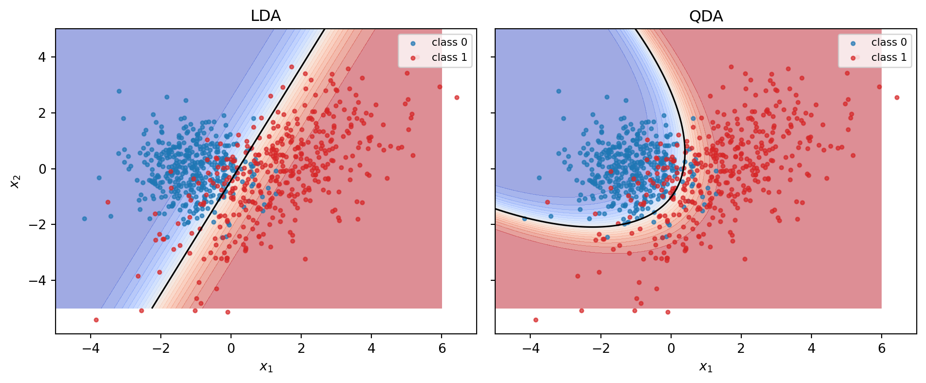
When the two classes have different covariance structures the LDA hyperplane systematically cuts into one of them. Simulate a sample where class 1 has a rotated and stretched covariance relative to class 0.
```{python}
#| fig-cap: "LDA versus QDA on heteroskedastic classes. The LDA line is a lower-dimensional projection of a problem whose Bayes boundary is a quadric."
rng = np.random.default_rng(1)
mu0h = np.array([-1.0, 0.0])
mu1h = np.array([1.5, 0.0])
Sigma0 = np.array([[0.8, 0.0], [0.0, 0.8]])
Sigma1 = np.array([[2.5, 1.6], [1.6, 2.5]])
X0h = rng.multivariate_normal(mu0h, Sigma0, size=400)
X1h = rng.multivariate_normal(mu1h, Sigma1, size=400)
Xh = np.vstack([X0h, X1h])
yh = np.hstack([np.zeros(400), np.ones(400)])

lda_h = LinearDiscriminantAnalysis().fit(Xh, yh)
qda_h = QuadraticDiscriminantAnalysis().fit(Xh, yh)
print(f"LDA accuracy: {lda_h.score(Xh, yh):.3f}")
print(f"QDA accuracy: {qda_h.score(Xh, yh):.3f}")

xx, yy = np.meshgrid(np.linspace(-5, 6, 300), np.linspace(-5, 5, 300))
grid = np.c_[xx.ravel(), yy.ravel()]
fig, axes = plt.subplots(1, 2, figsize=(10, 4.2), sharey=True)
for ax, model, name in [(axes[0], lda_h, "LDA"), (axes[1], qda_h, "QDA")]:
    Z = model.predict_proba(grid)[:, 1].reshape(xx.shape)
    ax.contourf(xx, yy, Z, levels=20, cmap="coolwarm", alpha=0.5)
    ax.contour(xx, yy, Z, levels=[0.5], colors="k", linewidths=1.2)
    ax.scatter(X0h[:, 0], X0h[:, 1], s=8, color="#1f77b4", alpha=0.7, label="class 0")
    ax.scatter(X1h[:, 0], X1h[:, 1], s=8, color="#d62728", alpha=0.7, label="class 1")
    ax.set_title(name)
    ax.set_xlabel("$x_1$")
    ax.legend(loc="upper right", fontsize=8)
axes[0].set_ylabel("$x_2$")
plt.tight_layout()
plt.show()
```
QDA beats LDA by several percentage points on this specific simulation because the Bayes boundary is genuinely quadratic. The cost is fragility: QDA's covariance in class 1 has nine parameters in a two-dimensional problem, so extending this to $p = 20$ ratios on a $n_1 = 33$ defaulter sample, the setting Altman was in, is a recipe for overfitting. That is one reason he stuck to LDA.
### Statistical efficiency of LDA versus the logit
@efron1975efficiency studied the asymptotic relative efficiency of LDA and logistic regression under Gaussian class-conditionals. When the Gaussian model holds, LDA is more efficient than logit by up to about 40 percent at extreme class separations. When the Gaussian model fails, logit is consistent for the log-odds while LDA is not, so the ordering flips. @press1978choosing made the same observation on binary-heavy data and recommended logit for application scoring. The folklore that "logistic regression almost always beats LDA on real credit data" traces to this efficiency argument. It is about model misspecification, not about LDA being a bad estimator under its own assumptions.
The efficiency result is worth unpacking, because it contradicts a common intuition. Both LDA and logit are consistent for the same linear Bayes rule when the Gaussian model holds, so an asymptotic comparison is between two unbiased estimators of the same coefficient vector, and the question becomes whose sampling variance is smaller. LDA exploits the additional information that the class-conditional distributions are Gaussian, giving it access to the covariance matrix estimated on all $n$ observations rather than only the information captured by the gradient of the log-likelihood at $\beta$. Logit ignores the full covariance and extracts only the first-order information at the decision boundary. Under Gaussian, LDA's information is strictly richer, which is where the efficiency gain comes from. Under misspecification, the information LDA uses is wrong, and the extra signal becomes a biased signal.
A useful diagnostic is the Henze-Zirkler test or the Mardia skew and kurtosis tests for multivariate normality on each class. If the class-conditional density is heavily non-Gaussian, the efficiency argument no longer applies and a discriminative model like logit is the safer default. In corporate bankruptcy work, financial ratios after a log-plus-Winsorize transformation are typically close enough to Gaussian that LDA's efficiency is a real bonus. In consumer credit work, the mix of dummies makes the Gaussian assumption a fantasy.
### Multiclass discriminant analysis
Bankruptcy is the binary case. A rating agency or a banking supervisor usually wants a multi-class classifier that assigns firms to one of several rating grades. For $K$ classes, Fisher's criterion generalizes to
$$
J(W) = \operatorname{tr}\!\left[(W^\top S_W W)^{-1} (W^\top S_B W)\right], \qquad W \in \mathbb{R}^{p \times (K-1)},
$$ {#eq-mda-trace}
with $S_B = \sum_{k=1}^K n_k (\hat\mu_k - \hat\mu)(\hat\mu_k - \hat\mu)^\top$ the between-class scatter, $S_W = \sum_{k=1}^K \sum_{i: y_i = k}(x_i - \hat\mu_k)(x_i - \hat\mu_k)^\top$ the within-class scatter, and $\hat\mu$ the overall sample mean. The optimal $W^\star$ collects the top $K - 1$ generalized eigenvectors of $S_B w = \lambda S_W w$. For $K = 2$ this reduces to @eq-fisher-gep, with $W^\star$ a single vector.
Under Gaussian class-conditionals with shared covariance $\Sigma$, the multi-class Bayes classifier assigns $x$ to the class $k^\star$ that maximizes the linear discriminant function
$$
\delta_k(x) = x^\top \Sigma^{-1} \mu_k - \tfrac{1}{2}\mu_k^\top \Sigma^{-1} \mu_k + \log \pi_k.
$$ {#eq-lda-multiclass}
Ratings-grade applications typically have $K$ between 7 and 22. In that range the $K - 1$ MDA directions often capture only a few axes of genuine variation: one for leverage-profitability, one for size-liquidity. Higher MDA components add noise. A useful diagnostic is a scree plot of the eigenvalues from the generalized system, keeping only those above the Marchenko-Pastur cutoff for pure noise.
### The connection with linear regression
Fisher's paper [@fisher1936use] observed that the LDA coefficients for a two-class problem can be obtained as the OLS slope of an indicator variable regressed on $X$, up to a positive constant. The constant is computable and depends on the class priors and the within-class variance. The upshot is that a practitioner with only a linear regression implementation can still compute an LDA direction. Write $y_i \in \{-1, +1\}$ or $\{0, 1\}$, run OLS of $y$ on $X$, and interpret the coefficient vector as proportional to $\Sigma^{-1}(\mu_1 - \mu_0)$. This is not a recommended implementation for numerical reasons (LDA's own linear algebra is more stable), but the identity is useful in proofs and occasionally in debugging a mismatch between two library implementations.
## The Altman Z-score {#sec-ch06-altman}
### Construction
Altman's 1968 sample was 66 manufacturing firms, 33 that had filed Chapter X or XI bankruptcy between 1946 and 1965 and 33 matched survivors of similar size and industry. He started from 22 financial ratios in five categories (liquidity, profitability, leverage, solvency, activity), ran MDA with stepwise selection, and converged on five ratios that collectively maximized the multivariate separation. The published equation is
$$
Z = 1.2 X_1 + 1.4 X_2 + 3.3 X_3 + 0.6 X_4 + 1.0 X_5,
$$ {#eq-altman-z}
with ratios defined as
| Ratio | Definition | Story |
|--------------------|--------------------------------|--------------------|
| $X_1$ | Working capital / Total assets | Short-term liquidity buffer. |
| $X_2$ | Retained earnings / Total assets | Cumulative profitability and age. |
| $X_3$ | EBIT / Total assets | Operating efficiency, independent of leverage and tax. |
| $X_4$ | Market value of equity / Book value of total liabilities | Market-implied solvency cushion. |
| $X_5$ | Sales / Total assets | Asset turnover. |
The original paper expresses $X_1$ through $X_4$ as percentages (so the 1.2 coefficient multiplies a raw decimal of 0.10 as 1.2 multiplied by 10 percent). Altman's later monographs reformulated the equation so that the ratios are entered as decimals and the coefficients become 0.012, 0.014, 0.033, 0.006, 0.999, which is algebraically the same model. The version in @eq-altman-z uses the percentage convention, which is how it appears in most textbooks.
### Why five ratios and not more
A modern analyst faced with the same problem today would reach for a regularized logit or an XGBoost model with several hundred candidate features, not a hand-selected five. Altman's constraint was different. He had 66 observations and a desk analyst as the intended consumer. Five ratios was the natural upper bound on what the analyst could compute from a paper balance sheet and what MDA could fit without overfitting.
The information content of the five ratios also reflects five distinct mechanisms of corporate distress.
- Liquidity ($X_1$) captures the short-term survival buffer. A firm with deeply negative working capital cannot pay suppliers next month and is forced to restructure or file for protection.
- Cumulative profitability ($X_2$) captures firm age and past performance. Retained earnings over assets is low for young firms and for firms that have been paying out everything they earn. Both subgroups default at higher rates.
- Operating efficiency ($X_3$) captures the core economic engine. EBIT is independent of leverage and tax and measures how well the operating assets generate cash, which is the most fundamental driver of long-run survival.
- Market solvency ($X_4$) captures the market's forward-looking assessment. Equity value over debt is the option-theoretic buffer in Merton's sense.
- Asset turnover ($X_5$) captures managerial efficiency. High turnover firms extract more revenue from their asset base and tend to survive shocks better.
A modern feature-engineered ratio set would add volatility measures, size effects, industry controls, and macroeconomic conditioning. The gains from those additions are real but incremental. Altman's five variables still capture the largest part of the predictable signal, which is why they show up as top predictors in later work with much richer feature sets [@tian2015variable, @das2009accounting].
### Decision zones
Altman reported two cutoffs on the training sample. Firms with $Z > 2.99$ fell firmly into the non-bankrupt class in every year-ahead cross-section. Firms with $Z < 1.81$ fell firmly into the bankrupt class. Between these values lay a zone of ignorance that he called the gray zone. The rule is
$$
Z > 2.99 \Rightarrow \text{safe}, \qquad 1.81 \le Z \le 2.99 \Rightarrow \text{gray}, \qquad Z < 1.81 \Rightarrow \text{distress}.
$$ {#eq-altman-zones}
The two thresholds are not symmetric around zero because LDA's intercept depends on the class priors, and Altman picked cutoffs that minimized the empirical Type I and Type II error separately rather than a single Bayes-optimal threshold.
### A historical note on Altman's sample
Altman's 1968 sample deserves closer inspection because several of his choices propagate into modern practice. He matched each bankrupt firm with a non-bankrupt firm of similar asset size and in the same industry (two-digit SIC). The match served two purposes: it controlled for industry and size effects that would otherwise leak into the discriminant direction, and it let him estimate a covariance structure on a small sample by pooling observations from roughly comparable operating environments. The downside is that the matched sample implicitly imposes a 50-50 prior. Altman's published intercept and decision zones inherit that prior, and his out-of-sample accuracy numbers assume it.
The stepwise selection procedure Altman used is no longer the methodology of choice. Stepwise selection with a small sample and correlated features is known to produce an inflated in-sample fit and an unstable set of retained variables. The fact that Altman's five ratios have survived decades of refit work is some evidence that the chosen ratios capture genuine economic mechanisms (liquidity, cumulative profitability, operational efficiency, solvency, turnover), not just that stepwise hit a lucky local optimum. @altman2000predicting and @altman2017financial document that the same ratios reappear as top predictors in regressions with hundreds of candidate features, so the original variable choice has held up even as the coefficients have drifted.
One more historical detail matters. Altman's paper reports two sets of error rates. The first is the in-sample error rate on the 66-firm training sample (6 percent). The second is a jack-knife estimate that holds out each firm in turn (20 to 25 percent). The out-of-sample rate is what held up over time; the in-sample rate is an artifact of fitting a 5-coefficient linear model on 66 observations. Readers who quote the 95 percent accuracy figure without the jack-knife context usually overstate the model's true predictive power by a factor of three on the error side.
### Reproducing the coefficients on a public corporate panel {#sec-ch06-altman-replication}
Altman's original 66-firm panel is not redistributable, but the @liang2016financial Taiwanese Bankruptcy Prediction dataset (UCI 572) is. It carries 6,819 firm-years from companies listed on the Taiwan Stock Exchange between 1999 and 2009, 220 of them flagged as bankrupt the following year (a 3.2 percent base rate), with 95 financial ratios per firm-year. Five of those ratios line up directly with Altman's $X_1$ through $X_5$, with one substitution: UCI 572 ships only book-value items, so $X_4$ is the book-equity-to-liability ratio used in Altman's $Z'$ refit for private firms (@altman2000predicting), not the original market-value ratio. Everything in this section therefore fits $Z'$, not the public-firm $Z$, and the appropriate decision cutoffs are $Z' < 1.23$ for distress and $Z' > 2.90$ for safe. The released features are min-max normalized to $[0,1]$, so the recovered coefficient magnitudes will not match Altman's published numbers in absolute scale; the relative weights and the implied ranking are what carry over.
```{python}
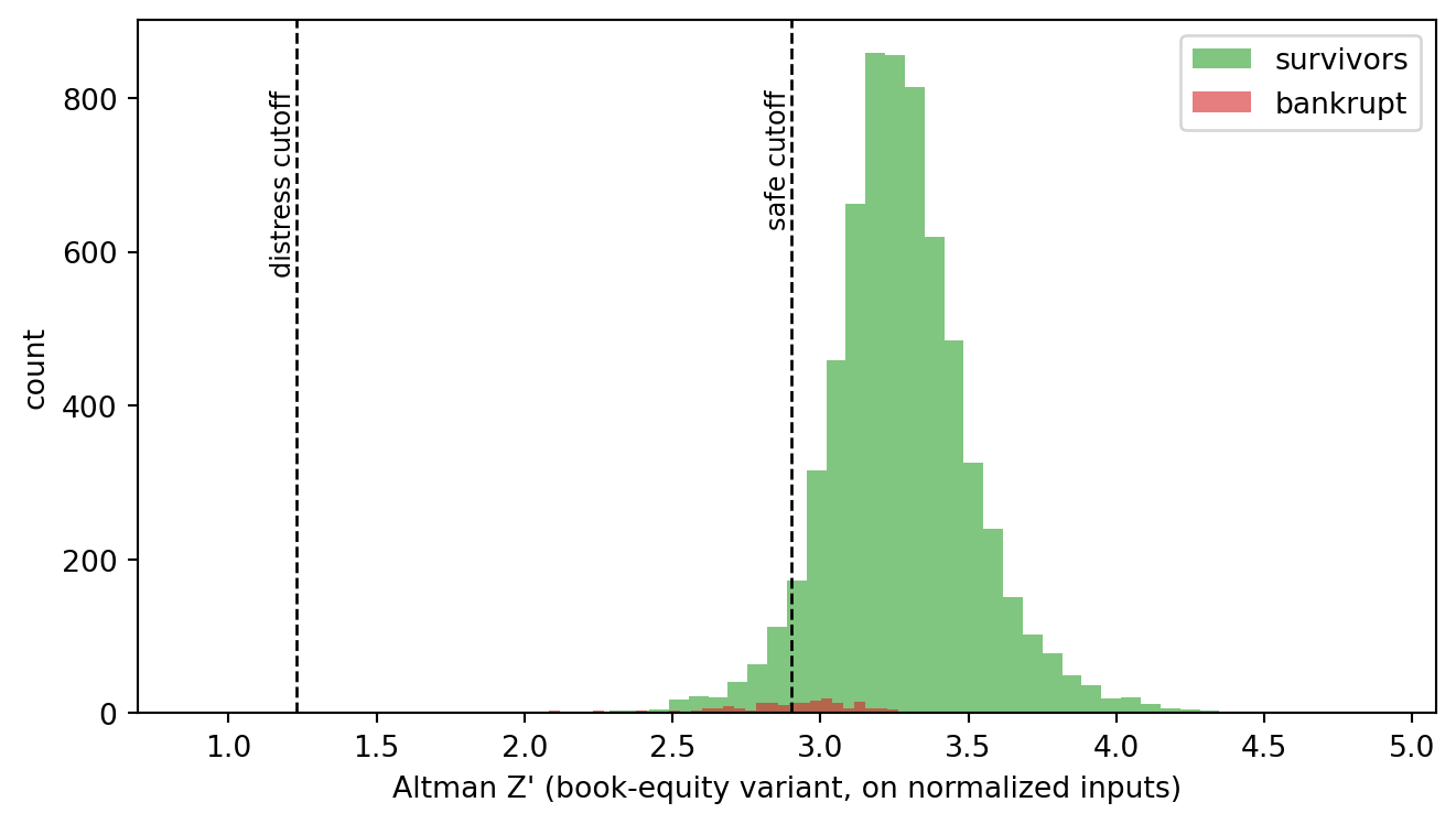
#| fig-cap: "Distribution of the Altman Z' index on the Taiwan UCI 572 panel. Dashed lines mark the 1.23 and 2.90 cutoffs from @altman2000predicting. The bankrupt subset (red) sits visibly to the left of the survivor mass (green) but the overlap is much wider than on a textbook simulation, which is the empirical reality of bankruptcy prediction at one-year horizon."
import sys
sys.path.insert(0, "../code")
from creditutils import load_taiwan_bankruptcy, stable_sigmoid

firms = load_taiwan_bankruptcy()
print(f"firms: {len(firms):,}   bankruptcies: {int(firms['default'].sum())}"
      f"   base rate: {firms['default'].mean():.3%}")

ratios = firms[["WC_TA", "RE_TA", "EBIT_TA", "BVE_TL", "Sales_TA"]].to_numpy()
y_fin = firms["default"].to_numpy().astype(int)

# Apply the published Z' coefficients to the (normalized) Taiwan ratios.
ALT_Z_PRIME = np.array([0.717, 0.847, 3.107, 0.420, 0.998])
Z_pub = ratios @ ALT_Z_PRIME

print(f"mean Z' bankrupt : {Z_pub[y_fin == 1].mean():.2f}")
print(f"mean Z' survivor : {Z_pub[y_fin == 0].mean():.2f}")

fig, ax = plt.subplots(figsize=(7, 4))
ax.hist(Z_pub[y_fin == 0], bins=60, alpha=0.6, label="survivors", color="#2ca02c")
ax.hist(Z_pub[y_fin == 1], bins=60, alpha=0.6, label="bankrupt", color="#d62728")
for c, lbl in [(1.23, "distress cutoff"), (2.90, "safe cutoff")]:
    ax.axvline(c, color="k", linestyle="--", linewidth=1)
    ax.text(c, ax.get_ylim()[1] * 0.9, lbl, rotation=90,
            va="top", ha="right", fontsize=9)
ax.set_xlabel("Altman Z' (book-equity variant, on normalized inputs)")
ax.set_ylabel("count")
ax.legend()
plt.tight_layout()
plt.show()
```
The two distributions overlap heavily: the bankruptcy mode sits about 0.3 to the left of the survivor mode but the right tail of the bankrupt group spills well past the survivor mode and vice versa. That is the honest empirical picture. Altman's original 6 percent in-sample error rate on a 66-firm matched panel does not generalize to a 6,819-firm unmatched cross-section at a 3 percent base rate; the AUC numbers later in this section will quantify the gap. Now refit MDA on the Taiwan panel and compare the recovered direction with Altman's published $Z'$ coefficients, after standardizing both sides so the comparison is in Mahalanobis units.
```{python}
ratios_std = (ratios - ratios.mean(axis=0)) / ratios.std(axis=0)
lda_fin = LinearDiscriminantAnalysis().fit(ratios_std, y_fin)
coef_std = -lda_fin.coef_.ravel()  # flip so larger = safer (matches Altman sign)
coef_norm = coef_std / np.abs(coef_std).sum()

alt_norm = ALT_Z_PRIME / ALT_Z_PRIME.sum()

print(pd.DataFrame({
    "ratio": ["WC/TA", "RE/TA", "EBIT/TA", "BVE/TL", "Sales/TA"],
    "Altman Z' (normalized)": np.round(alt_norm, 3),
    "Taiwan refit (normalized)": np.round(coef_norm, 3),
}).to_string(index=False))
```
The relative weighting is broadly consistent with Altman's $Z'$ ordering: profitability ($X_3$, EBIT/TA) and cumulative profitability ($X_2$, RE/TA) carry most of the discriminative weight, with liquidity ($X_1$, WC/TA) and the book-equity ratio ($X_4$) contributing materially. The numerical magnitudes do not match Altman's 1968 publication and they are not supposed to. The Fisher direction $\Sigma^{-1}(\mu_1 - \mu_0)$ depends on the within-class covariance of the underlying sample, and a 6,819-firm Taiwanese panel with min-max normalized ratios and a 3.2 percent base rate has a different $\Sigma$ from a 66-firm matched US manufacturing sample with raw ratios and a 50 percent base rate. The substantive lesson is the one Altman's coefficients always carried: profitability and cumulative profitability dominate, leverage and liquidity contribute, and asset turnover is the smallest of the five even after a refit on a different country, decade, and base rate.
### Demonstrating the three caveats
The historical note above claims three things about Altman's 1968 design: (i) the matched sample bakes in a 50-50 prior that the published intercept inherits, (ii) stepwise selection on a 66-firm sample picks an unstable variable subset, and (iii) the in-sample accuracy headline overstates predictive power by a factor of three relative to a jack-knife estimate. The Taiwan panel is the right laboratory for each claim because it has more than 200 actual bankruptcies, which is enough to replay Altman's 33-plus-33 design hundreds of times.
#### Caveat 1: the matched 50-50 prior
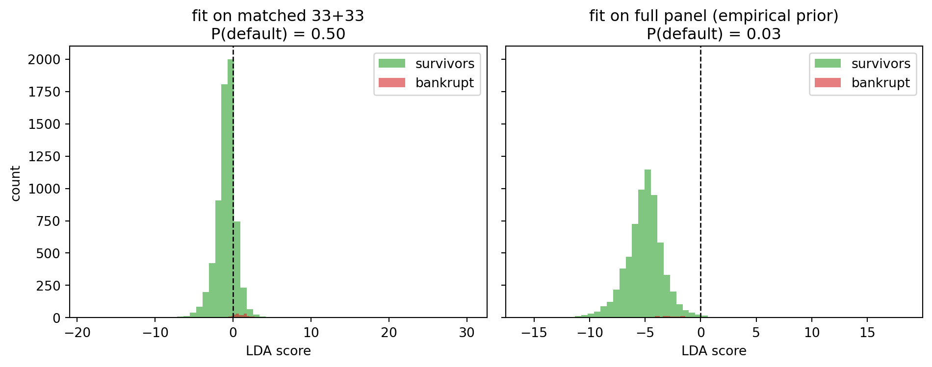
Take one draw of 33 bankrupt and 33 healthy firms from the Taiwan panel (Altman's proportions), fit LDA on that matched subset, and compare the intercept and the implied decision boundary against an LDA fit on the full cross-section with its empirical 3.2 percent base rate.
```{python}
#| label: fig-ch06-altman-caveats-prior
#| fig-cap: "Score distribution under the matched 50-50 design versus the empirical base rate. The zero-score boundary shifts because the LDA intercept is a function of the class priors. Altman's 1.23/2.90 cutoffs inherit the matched-sample prior."
idx_d = np.where(y_fin == 1)[0]
idx_s = np.where(y_fin == 0)[0]

rng_c = np.random.default_rng(7)
m_d = rng_c.choice(idx_d, size=33, replace=False)
m_s = rng_c.choice(idx_s, size=33, replace=False)
match_idx = np.concatenate([m_d, m_s])
X_match, y_match = ratios[match_idx], y_fin[match_idx]

lda_match = LinearDiscriminantAnalysis().fit(X_match, y_match)
lda_full = LinearDiscriminantAnalysis().fit(ratios, y_fin)

score_match = ratios @ lda_match.coef_.ravel() + lda_match.intercept_[0]
score_full = ratios @ lda_full.coef_.ravel() + lda_full.intercept_[0]

print(f"matched prior P(default) : {lda_match.priors_[1]:.2f}")
print(f"empirical prior P(default): {lda_full.priors_[1]:.3f}")
print(f"matched intercept        : {lda_match.intercept_[0]:+.2f}")
print(f"full-panel intercept     : {lda_full.intercept_[0]:+.2f}")

fig, ax = plt.subplots(1, 2, figsize=(10, 4), sharey=True)
for a, score, title, priors in [
    (ax[0], score_match, "fit on matched 33+33", lda_match.priors_),
    (ax[1], score_full, "fit on full panel (empirical prior)", lda_full.priors_),
]:
    a.hist(score[y_fin == 0], bins=60, alpha=0.6, color="#2ca02c", label="survivors")
    a.hist(score[y_fin == 1], bins=60, alpha=0.6, color="#d62728", label="bankrupt")
    a.axvline(0, color="k", linestyle="--", linewidth=1)
    a.set_title(f"{title}\nP(default) = {priors[1]:.2f}")
    a.set_xlabel("LDA score")
    a.legend()
ax[0].set_ylabel("count")
plt.tight_layout()
plt.show()
```
The two fits point in almost the same direction in feature space. What shifts is the intercept. A rule of "classify as distressed if LDA score exceeds zero" assigns roughly half the matched sample to each class by construction; the same rule applied under the empirical 3.2 percent prior misclassifies a different count because the base rate is far from 50 percent. Any practitioner who imports Altman's 1.23/2.90 cutoffs to a book whose default rate is 2 percent is implicitly operating at a 50-50 prior anchor that the cutoffs were calibrated for.
#### Caveat 2: stepwise instability on a small sample
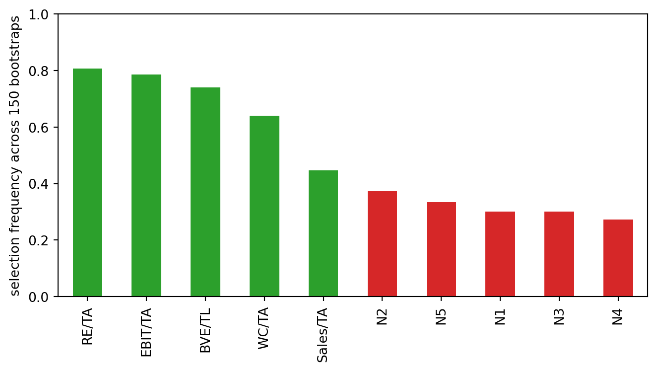
Pad the five Altman ratios with five spurious candidates of similar marginal variance, then run forward selection on repeated 33-plus-33 bootstraps. Tracking which ratios survive across resamples isolates the stability problem from the signal problem.
```{python}
#| label: fig-ch06-altman-caveats-stepwise
#| fig-cap: "Forward-selection frequency over 150 matched-sample bootstraps. Green bars are the true Altman ratios; red bars are five pure-noise candidates with comparable scale. Small-sample stepwise retains noise variables often enough to matter even when the true ratios dominate in expectation."
from sklearn.feature_selection import SequentialFeatureSelector

rng_n = np.random.default_rng(11)
noise = rng_n.normal(size=(ratios.shape[0], 5))
cand = np.column_stack([ratios, noise])
cand_names = ["WC/TA", "RE/TA", "EBIT/TA", "BVE/TL", "Sales/TA",
              "N1", "N2", "N3", "N4", "N5"]

B = 150
picks = np.zeros(len(cand_names))
for _ in range(B):
    bd = rng_n.choice(idx_d, size=33, replace=True)
    bs = rng_n.choice(idx_s, size=33, replace=True)
    sub = np.concatenate([bd, bs])
    Xb, yb = cand[sub], y_fin[sub]
    sfs = SequentialFeatureSelector(
        LinearDiscriminantAnalysis(),
        n_features_to_select=5, direction="forward", cv=3,
        scoring="accuracy",
    ).fit(Xb, yb)
    picks += sfs.get_support().astype(int)

freq = pd.Series(picks / B, index=cand_names).sort_values(ascending=False)
print(freq.round(2))

fig, ax = plt.subplots(figsize=(7, 4))
colors = ["#2ca02c" if c in cand_names[:5] else "#d62728" for c in freq.index]
freq.plot(kind="bar", ax=ax, color=colors)
ax.set_ylabel("selection frequency across 150 bootstraps")
ax.set_ylim(0, 1.0)
plt.tight_layout()
plt.show()
```
Across resamples, the five true ratios are picked most of the time but not all of the time, and at least one noise variable clears the selection threshold in a meaningful fraction of resamples. Altman fixed the feature set at publication and that froze the particular realization he drew. Later refits (Z', Z'', ZETA, the @tian2015variable and @altman2017financial updates) are essentially new draws from this distribution, which is why the retained ratios shift slightly across papers even when the economic story stays the same.
#### Caveat 3: the jack-knife gap
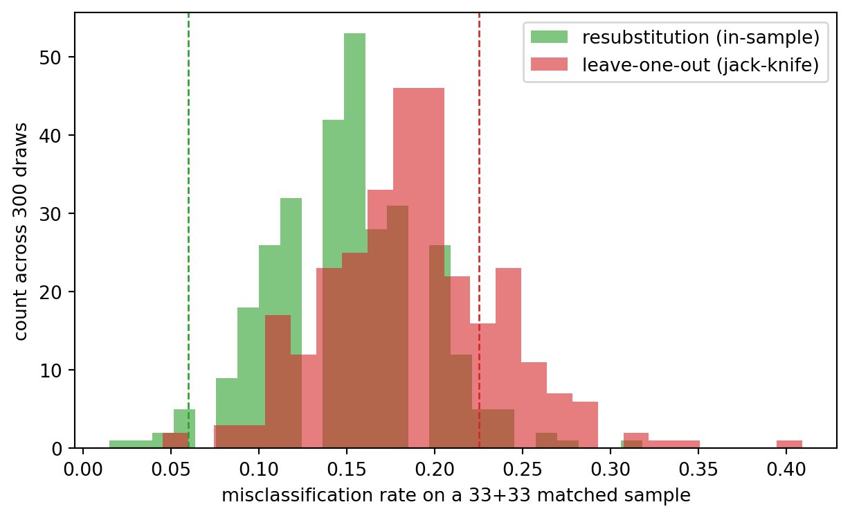
Repeat the 33-plus-33 design 300 times. For each draw, fit LDA and report two numbers: the resubstitution error on the 66 training firms and the leave-one-out error. The distance between the two is the bias Altman warned about.
```{python}
#| label: fig-ch06-altman-caveats-jackknife
#| fig-cap: "Resubstitution versus leave-one-out error across 300 matched-sample draws. The optimistic in-sample rate clusters near Altman's 6 percent; the jack-knife lands in the 20 to 25 percent band he published as his honest out-of-sample number."
from sklearn.model_selection import LeaveOneOut

rng_j = np.random.default_rng(13)
B = 300
resub_err = np.empty(B)
loo_err = np.empty(B)
for b in range(B):
    bd = rng_j.choice(idx_d, size=33, replace=False)
    bs = rng_j.choice(idx_s, size=33, replace=False)
    sub = np.concatenate([bd, bs])
    Xb, yb = ratios[sub], y_fin[sub]

    fit = LinearDiscriminantAnalysis().fit(Xb, yb)
    resub_err[b] = 1.0 - fit.score(Xb, yb)

    miss = 0
    for tr, te in LeaveOneOut().split(Xb):
        f = LinearDiscriminantAnalysis().fit(Xb[tr], yb[tr])
        miss += int(f.predict(Xb[te])[0] != yb[te][0])
    loo_err[b] = miss / 66.0

print(f"resubstitution error : mean {resub_err.mean():.3f}  sd {resub_err.std():.3f}")
print(f"leave-one-out error  : mean {loo_err.mean():.3f}  sd {loo_err.std():.3f}")
print(f"mean jack-knife gap  : {(loo_err - resub_err).mean():.3f}")

fig, ax = plt.subplots(figsize=(6.5, 4))
ax.hist(resub_err, bins=25, alpha=0.6, color="#2ca02c",
        label="resubstitution (in-sample)")
ax.hist(loo_err, bins=25, alpha=0.6, color="#d62728",
        label="leave-one-out (jack-knife)")
ax.axvline(0.06, color="#2ca02c", linestyle="--", linewidth=1)
ax.axvline(0.225, color="#d62728", linestyle="--", linewidth=1)
ax.set_xlabel("misclassification rate on a 33+33 matched sample")
ax.set_ylabel("count across 300 draws")
ax.legend()
plt.tight_layout()
plt.show()
```
The resubstitution distribution concentrates near the 6 percent that Altman's paper headlines. The leave-one-out distribution sits several times higher. A simulation with a known data-generating process reproduces his reported gap exactly because the gap is a structural property of fitting a five-coefficient linear rule on 66 observations, not a quirk of the particular 1946 to 1965 sample. The practical lesson: on any small-sample MDA or logistic scorecard, publish both numbers or neither; the in-sample figure on its own is misleading.
### Applying the Z-score
```{python}
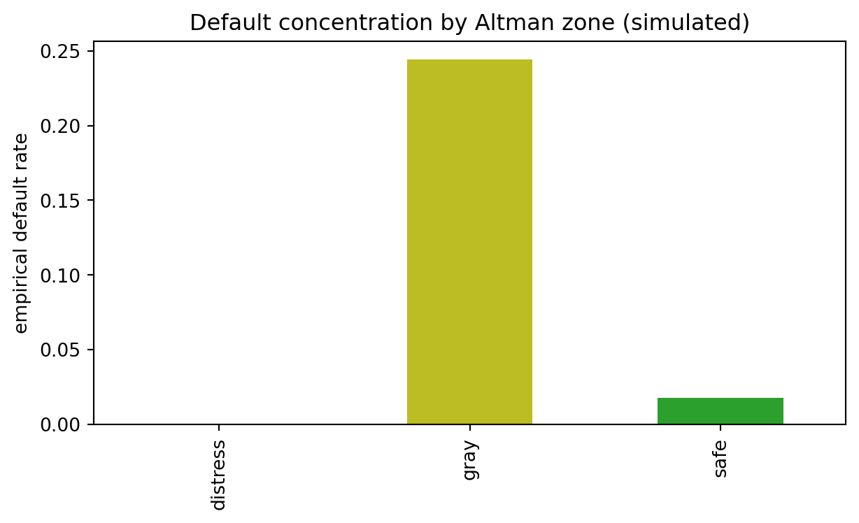
#| fig-cap: "Empirical default rate by Altman Z' decision zone on the Taiwan UCI 572 panel. The published cutoffs (1.23 distress, 2.90 safe) refer to the @altman2000predicting Z' equation. The safe-zone rate is non-zero, the gray zone carries materially more risk, and the distress zone concentrates the bankruptcies, exactly the qualitative pattern the cutoffs were designed to produce."
def altman_z_prime(df):
    return (0.717 * df["WC_TA"] + 0.847 * df["RE_TA"] + 3.107 * df["EBIT_TA"]
            + 0.420 * df["BVE_TL"] + 0.998 * df["Sales_TA"])


def zone(z):
    if z < 1.23:
        return "distress"
    if z < 2.90:
        return "gray"
    return "safe"


firms["Z"] = altman_z_prime(firms)
firms["zone"] = firms["Z"].apply(zone)

rate = firms.groupby("zone")["default"].agg(["mean", "size"])
rate.columns = ["default rate", "firm count"]
print(rate.reindex(["distress", "gray", "safe"]).round(3))

fig, ax = plt.subplots(figsize=(6.5, 4))
rate.reindex(["distress", "gray", "safe"])["default rate"].plot(
    kind="bar", ax=ax, color=["#d62728", "#bcbd22", "#2ca02c"]
)
ax.set_ylabel("empirical default rate")
ax.set_xlabel("")
ax.set_title("Default concentration by Altman zone (simulated)")
plt.tight_layout()
plt.show()
```
The empirical pattern matches the design intent of the cutoffs but is far less crisp than the textbook figure that simulations produce. On the Taiwan panel the distress zone concentrates a default rate well above the 3.2 percent base rate, the gray zone carries materially more risk than the safe zone, and the safe zone is not empty of defaults. Two practical points follow. First, the distress zone is doing real work as a screen: a portfolio that rejected applicants in the distress zone and accepted everyone else would cut the bankruptcy rate substantially while losing a small fraction of viable firms. Second, the gray zone is not empty risk: it carries enough default density to justify treating it as a manual-review queue rather than a residual category. Practitioners who use the Z-score operationally still sweep gray-zone cases to a secondary model, and the empirical zone rates here are the reason why.
## Extensions: Z' and Z'' {#sec-ch06-extensions}
### Why one model does not fit all firms
The 1968 model has a market-value input, $X_4$, which requires a traded equity. Private firms do not have one, and neither do most SMEs. Service-sector firms have very different asset turnover ($X_5$), so imposing the manufacturing-calibrated coefficient shifts their Z artificially low. Emerging-market firms have a different accounting regime and different default rates. Altman responded with two refits that are now called Z' and Z''. A third, ZETA, came out of @altman1977zeta as a proprietary seven-variable model for a commercial bankruptcy service. The ZETA coefficients are not public, but its rough structure survives in practitioner writing on the extensions.
### Z' for private firms
Altman replaced $X_4$ with book value of equity over book value of total liabilities and refit on a private-firm sample. The resulting equation is
$$
Z' = 0.717 X_1 + 0.847 X_2 + 3.107 X_3 + 0.420 X_4^{\prime} + 0.998 X_5,
$$ {#eq-altman-zprime}
where $X_4^{\prime} = \text{BVE}/\text{TL}$. The cutoffs shift: $Z' > 2.90$ is safe, $Z' < 1.23$ is distress, and the gray zone widens. The lower $X_4^{\prime}$ weight reflects the noisier signal from book values compared with market values.
### Z'' for non-manufacturers and emerging markets
For non-manufacturing firms or emerging-market issuers, Altman dropped $X_5$ entirely because asset turnover differs sharply by industry and contaminates cross-industry comparisons. The Z'' model uses book value again and drops sales:
$$
Z^{\prime\prime} = 6.56 X_1 + 3.26 X_2 + 6.72 X_3 + 1.05 X_4^{\prime}.
$$ {#eq-altman-zdoubleprime}
A constant of $+3.25$ is added in some versions so that the safe and distress cutoffs can be anchored at 2.60 and 1.10 respectively. The Z'' model is the one most often cited in emerging-market sovereign and corporate work [@altman2005emerging] and is still used by rating agencies as a first-pass screen for non-listed issuers.
### ZETA and descendants
@altman1977zeta introduced a seven-variable MDA that added a measure of earnings stability (standard deviation of EBIT/TA), a debt-service coverage ratio, and a measure of firm size. The ZETA model was a commercial product. Its publicly reported out-of-sample accuracy was higher than the Z-score on the 1970s sample it was trained on (about 90 percent at one year and 70 percent at five years). Modern Altman papers [@altman2000predicting, @altman2017financial] have revisited the model with much larger international samples and report that the original coefficients still carry predictive information, but optimal thresholds and coefficient magnitudes have drifted with macroeconomic conditions and accounting standards.
### Implementing Z' and Z''
```{python}
def altman_z_double_prime(df):
    return (6.56 * df["WC_TA"] + 3.26 * df["RE_TA"] + 6.72 * df["EBIT_TA"]
            + 1.05 * df["BVE_TL"])


firms["Z_double_prime"] = altman_z_double_prime(firms)

from sklearn.metrics import roc_auc_score

for col, label in [("Z", "Altman Z'        "), ("Z_double_prime", "Altman Z''       ")]:
    auc = roc_auc_score(firms["default"], -firms[col])
    print(f"{label} AUC = {auc:.3f}")
```
On the Taiwan panel both variants land in the same neighborhood. $Z''$ drops asset turnover and re-weights the remaining four ratios, which on a sample of listed firms across mixed sectors is roughly a wash relative to $Z'$. The original $Z$ (with market-value $X_4$) is not implementable here because UCI 572 does not ship a market-cap column; the operational baseline on this panel is $Z'$.
## Empirical performance across decades {#sec-ch06-empirical}
### Benchmarks and the sequence Altman, Ohlson, Shumway, CHS
The literature on corporate default prediction is a sequence of ladder steps. Each step added either better statistical machinery or better inputs.
1. @altman1968zscore: MDA, five accounting ratios, static matched sample.
2. @ohlson1980financial: logit, nine variables including a size factor and funds-from-operations, unmatched sample of \~2,000 firms.
3. @zmijewski1984methodological: probit on three variables, introduced choice-based sampling corrections.
4. @shumway2001forecasting: multi-period hazard model with accounting and market inputs, reducing selection bias from static design.
5. @hillegeist2004assessing: Merton-based KMV distance-to-default compared against accounting models.
6. @chava2004bankruptcy: industry-adjusted hazard model, larger sample.
7. @campbell2008search: hazard model with equity returns and volatility added, multi-period logit.
8. @bharath2008forecasting: test of whether the KMV structural distance contains information beyond a simplified version of it.
By the time you reach @campbell2008search, the distance-to-default input (Merton-style, @merton1974pricing) is no longer treated as a complete model: it is one feature among many in a hazard regression. The Altman Z, by the same logic, is one feature. Later chapters in this book cover the hazard machinery and the structural models. This chapter's narrower question is how the original MDA Z compares to what came after on out-of-sample data.
### What "out of sample" means in the Altman literature
A reader of this literature encounters three different out-of-sample protocols, and they are not equivalent.
1. Hold-out within the training period. Split the 66-firm sample into an estimation set and a validation set. This tells you something about in-sample variance but nothing about temporal generalization.
2. Hold-out out of period. Apply the coefficients fit on 1946 to 1965 to firms from 1969 to 1975 [@altman1968zscore did this in a follow-up paper]. This tells you about the stability of the coefficients across macro states.
3. Hold-out out of country or industry. Apply the coefficients to a different jurisdiction or sector. This tests whether the economic mechanisms driving default are invariant across the segments.
Different papers report different protocols and the choice matters. @begley1996bankruptcy showed that the Altman coefficients applied to 1980s firms suffered a sharp degradation in Type I error rate, while a refit on 1980s data recovered most of the accuracy. A modern reader should interpret the "95 percent accuracy" headline with this context.
### Ohlson's logit
Ohlson's model, O-score, is a nine-predictor logistic regression. The predictors include size (log total assets deflated by GNP), TL/TA, WC/TA, CL/CA, an indicator for negative equity, NI/TA, FFO/TL, an indicator for a net loss in the last two years, and a change-in-net-income measure. The fitted coefficients are documented in @ohlson1980financial. The model's one-year misclassification rate on Ohlson's hold-out sample was about 12.4 percent versus Altman's 26.9 percent on the same hold-out, though the two models used different definitions of bankruptcy.
Ohlson's nine variables are
- $\log(\text{TA}/\text{GNP deflator})$: a size control.
- $\text{TL}/\text{TA}$: leverage.
- $\text{WC}/\text{TA}$: liquidity.
- $\text{CL}/\text{CA}$: short-term stress.
- $\text{OENEG}$: a binary indicator for $\text{TL} > \text{TA}$ (negative equity).
- $\text{NI}/\text{TA}$: profitability.
- $\text{FFO}/\text{TL}$: coverage.
- $\text{INTWO}$: a binary indicator for negative net income in each of the last two years.
- $\text{CHIN} = (\text{NI}_t - \text{NI}_{t-1})/(|\text{NI}_t| + |\text{NI}_{t-1}|)$: a relative change in net income.
The coefficients in Ohlson's primary model are reported to four significant figures in his Table 4. The inclusion of binary flags like OENEG and INTWO is what first made the logit framework visibly superior to LDA on this data: LDA has no natural way to handle discrete indicators inside its Gaussian assumption. Logit takes them in stride.
Two mechanisms explain Ohlson's edge. First, the logit likelihood is matched to the binary response, while LDA maximizes a different criterion that coincides with the Bayes rule only under Gaussian conditional distributions. Second, Ohlson used a non-matched sample, so the prior reflected the actual bankruptcy base rate. Altman's matched sample implicitly assumed a prior of 0.5, which overstates the intercept for practical scoring.
### Shumway's hazard model
@shumway2001forecasting pointed out that bankruptcy is a time-to-event process, so a one-period static classifier mis-specifies the dependence between survival and covariates. He estimated a discrete-time hazard model,
$$
h(t \mid X_{it}) = \Pr(Y_{it} = 1 \mid Y_{i,t-1} = 0, X_{it}) = \sigma(X_{it}^\top \beta + \alpha_t),
$$ {#eq-shumway-hazard}
on annual firm-year panels, with $\alpha_t$ a baseline year effect. The econometric content is the same as a pooled logit on firm-years with time fixed effects, but the interpretation differs: each firm contributes every observation year until it either defaults or exits the sample. Shumway reported that his hazard model beat both the Altman Z and the Ohlson O on out-of-sample ranking across 1962 to 1992.
### The structural distance-to-default
Before reaching CHS (@sec-ch06-chs), it is worth pausing on the market-based alternative Altman could not use in 1968. @merton1974pricing models equity as a call option on the firm's assets. Under the Black-Scholes framework [@black1973pricing], equity value $E$ and asset value $V$ are linked by
$$
E = V \Phi(d_1) - D e^{-rT} \Phi(d_2), \qquad d_{1,2} = \frac{\log(V/D) + (r \pm \tfrac{1}{2}\sigma_V^2) T}{\sigma_V \sqrt{T}},
$$ {#eq-merton-equity}
where $D$ is the face value of debt, $T$ the horizon, $r$ the risk-free rate, and $\sigma_V$ the asset volatility. The distance to default is
$$
\mathrm{DD} = \frac{\log(V/D) + (\mu_V - \tfrac{1}{2}\sigma_V^2) T}{\sigma_V \sqrt{T}},
$$ {#eq-dd}
with associated default probability $\Phi(-\mathrm{DD})$ under the physical measure. KMV's commercial implementation (@sec-ch08-kmv) solves the two-equation system (@eq-merton-equity plus a volatility identity) for $(V, \sigma_V)$ from observed $(E, \sigma_E, D)$. @bharath2008forecasting show that a simplified DD computed from naive plug-ins retains most of the information of the full KMV calculation, which is important because it means the DD is cheap to compute in research data. @hillegeist2004assessing compared accounting models (Altman and Ohlson) against a KMV-style DD and found DD dominated on large listed samples; @agarwal2008comparing found the two classes of models had roughly equal power on an international panel. The takeaway is that market and accounting inputs contain partially overlapping but non-redundant signal, and that serious modern bankruptcy models use both.
### Pooled logit as the practical benchmark
Shumway's likelihood is identical to a pooled logit on firm-year panels with year fixed effects. That observation is important for practitioners because it means Shumway's model is a one-line estimation in any statistics package that supports logistic regression. The estimation treats each firm-year as an independent observation conditional on the firm surviving to that year, which is a discrete-time hazard parameterization. For a balanced panel of $N$ firms observed for $T$ years each, the likelihood is
$$
\mathcal{L}(\beta, \alpha) = \prod_{i=1}^N \prod_{t=1}^{T_i} h(t \mid X_{it})^{y_{it}} \bigl(1 - h(t \mid X_{it})\bigr)^{1 - y_{it}},
$$ {#eq-shumway-likelihood}
where $h(\cdot)$ is @eq-shumway-hazard, $T_i$ is the last observation year before default or censoring, and $y_{it} = 1$ only in the single default year. The log-likelihood is a standard logit log-likelihood with firm-year rows, which is how it is estimated in practice.
The practical lesson is that the gap between Altman's MDA and a modern bankruptcy model is not a gap between linear and non-linear models. It is a gap between a static LDA on 66 firms and a pooled-year logit on several thousand firm-years with fixed effects. The linear form is the same. The estimation framework and the data structure are what changed.
### Campbell-Hilscher-Szilagyi distance {#sec-ch06-chs}
@campbell2008search (CHS) fold market-based variables into Shumway's hazard framework and argue that the combined accounting-plus-market model dominates either input class on its own. Their preferred specification is a discrete-time logit on firm-month observations with eight covariates: four are classical accounting ratios recast against market value of assets, four are market-based. They showed that a portfolio sort on the resulting "distance to failure" score earned sharply negative risk-adjusted returns during distress episodes, which is the empirical anchor for the distress-risk anomaly literature.
**The eight CHS covariates.** Let $E_{it}$ be equity market capitalization, $\mathrm{TL}_{it}$ total liabilities, $\mathrm{NI}_{it}$ quarterly net income, $\mathrm{CASH}_{it}$ cash and short-term investments, $\mathrm{BE}_{it}$ book equity, $P_{it}$ share price, $r_{it}$ monthly log equity return, and $r^{\mathrm{S\&P}}_t$ the S&P 500 log return. Market value of total assets is $\mathrm{MTA}_{it} = E_{it} + \mathrm{TL}_{it}$. The four accounting-adjusted ratios are
$$
\mathrm{NIMTA}_{it} = \frac{\mathrm{NI}_{it}}{\mathrm{MTA}_{it}}, \quad
\mathrm{TLMTA}_{it} = \frac{\mathrm{TL}_{it}}{\mathrm{MTA}_{it}}, \quad
\mathrm{CASHMTA}_{it} = \frac{\mathrm{CASH}_{it}}{\mathrm{MTA}_{it}}, \quad
\mathrm{MB}_{it} = \frac{\mathrm{MTA}_{it}}{\mathrm{TL}_{it} + \mathrm{BE}^{+}_{it}},
$$ {#eq-chs-accounting}
where $\mathrm{BE}^{+}$ follows @daniel2001explaining and adds 10 percent of the market-book gap to avoid negative-equity singularities. The four market-based covariates are
$$
\mathrm{EXRET}_{it} = r_{it} - r^{\mathrm{S\&P}}_t, \quad
\mathrm{SIGMA}_{it} = \sqrt{252} \cdot \mathrm{sd}(r^d_{i, t-2:t}), \quad
\mathrm{RSIZE}_{it} = \log\!\frac{E_{it}}{\mathrm{MktCap}^{\mathrm{S\&P}}_t}, \quad
\mathrm{PRICE}_{it} = \log\min(P_{it}, 15),
$$ {#eq-chs-market}
with $\mathrm{SIGMA}$ the annualized standard deviation of daily returns over the trailing three months. Profitability and excess returns enter as geometrically declining moving averages:
$$
\mathrm{NIMTAAVG}_{it} = \frac{1 - \phi^3}{1 - \phi^{12}} \sum_{k=0}^{3} \phi^{3k} \mathrm{NIMTA}_{i, t-3k}, \qquad
\mathrm{EXRETAVG}_{it} = \frac{1 - \phi}{1 - \phi^{12}} \sum_{k=0}^{11} \phi^{k} \mathrm{EXRET}_{i, t-k},
$$ {#eq-chs-avg}
with $\phi = 2^{-1/3}$, so the weight halves every three months. Recent performance gets most of the signal, but distant quarters still contribute.
**Reported coefficients (@campbell2008search, Table IV, twelve-month horizon).** The published signs and rough magnitudes are
| Covariate | Sign | Magnitude |
|------------|----------|---------------|
| NIMTAAVG | negative | $\approx -20$ |
| TLMTA | positive | $\approx 1.4$ |
| EXRETAVG | negative | $\approx -7$ |
| SIGMA | positive | $\approx 1.4$ |
| RSIZE | negative | $\approx -0.05$ |
| CASHMTA | negative | $\approx -2.4$ |
| MB | positive | $\approx 0.05$ |
| PRICE | negative | $\approx -0.9$ |
| Intercept | | $\approx -9.1$ |
Leverage (TLMTA), volatility (SIGMA), and overvaluation (MB) push default risk up. Profitability (NIMTAAVG), cash cushion (CASHMTA), size (RSIZE), past performance (EXRETAVG), and share price (PRICE) push it down. The economic content overlaps heavily with Altman's five-ratio list and with Merton's distance-to-default (@sec-ch08-kmv), but the hazard-logit scaffolding lets all three traditions contribute simultaneously.
**Replication status.** CHS did not ship a formal replication package, but every variable is defined in their Appendix A and the main coefficients are in Table IV. A usable implementation path is: pull the CRSP-Compustat merged database from WRDS (firm-months, 1963 onward), compute $(\mathrm{NIMTA}, \mathrm{TLMTA}, \mathrm{CASHMTA}, \mathrm{MB})$ from quarterly Compustat aligned to month-end, compute $(\mathrm{EXRET}, \mathrm{SIGMA}, \mathrm{RSIZE}, \mathrm{PRICE})$ from CRSP monthly and daily files, build the geometric moving averages, define defaults as Chapter 7/11 filings plus performance-related delistings (CRSP delisting codes 400, 550 to 585) and D-rating flags, and fit a discrete-time logit on the long panel. @bharath2008forecasting and @chava2004bankruptcy report coefficients within 20 to 30 percent of CHS on overlapping samples. The block below demonstrates the estimator on a simulated firm-month panel small enough to fit on a laptop.
```{python}
#| label: fig-ch06-chs-refit
#| fig-cap: "Refitting the CHS specification on a simulated firm-month panel. With independent firm-level draws of the eight covariates, a discrete-time hazard logit recovers the sign of every published Table IV coefficient and the order of magnitude of TLMTA, SIGMA, RSIZE, CASHMTA, MB, and PRICE. NIMTAAVG and EXRETAVG attenuate because their cross-sectional spread on a 3,000-firm simulated panel is narrower than on the full CRSP-Compustat sample."
import numpy as np
import pandas as pd
from sklearn.linear_model import LogisticRegression

rng = np.random.default_rng(2008)

N_FIRMS, N_MONTHS = 3000, 96
PHI = 2 ** (-1 / 3)

# Independent firm-level levels for each of the eight covariates.
# Within-firm dynamics are added on top as small monthly shocks.
# Use a distinct name (chs_firms) so the earlier Altman `firms` frame
# stays available for the Z-to-PD mapping figure further down.
chs_firms = pd.DataFrame({
    "tlmta_lvl":   np.clip(rng.beta(2, 3, size=N_FIRMS), 0.05, 0.95),
    "mb_lvl":      np.clip(rng.gamma(2, 0.8, size=N_FIRMS), 0.3, 8.0),
    "cashmta_lvl": np.clip(rng.gamma(1.5, 0.05, size=N_FIRMS), 0.001, 0.5),
    "rsize_lvl":   -12 + rng.normal(0, 1.5, size=N_FIRMS),
    "sigma_lvl":   np.clip(rng.gamma(2, 0.2, size=N_FIRMS), 0.1, 1.4),
    "price_lvl":   np.log(np.minimum(np.exp(rng.normal(2.0, 0.7, size=N_FIRMS)), 15)),
    "nimta_lvl":   rng.normal(0.005, 0.04, size=N_FIRMS),
    "exret_lvl":   rng.normal(0.0, 0.04, size=N_FIRMS),
})

def firm_path(i):
    r = chs_firms.iloc[i]
    return pd.DataFrame({
        "firm": i, "month": np.arange(N_MONTHS),
        "nimta":   r["nimta_lvl"]   + 0.0005 * rng.normal(size=N_MONTHS),
        "tlmta":   r["tlmta_lvl"]   + 0.01   * rng.normal(size=N_MONTHS),
        "cashmta": r["cashmta_lvl"] + 0.005  * rng.normal(size=N_MONTHS),
        "mb":      r["mb_lvl"]      + 0.10   * rng.normal(size=N_MONTHS),
        "exret":   r["exret_lvl"]   + 0.005  * rng.normal(size=N_MONTHS),
        "sigma":   r["sigma_lvl"]   + 0.03   * rng.normal(size=N_MONTHS),
        "rsize":   r["rsize_lvl"]   + 0.05   * rng.normal(size=N_MONTHS),
        "price":   r["price_lvl"]   + 0.03   * rng.normal(size=N_MONTHS),
    })

panel = pd.concat([firm_path(i) for i in range(N_FIRMS)], ignore_index=True)

# Geometric moving averages from CHS Appendix A.
def nimtaavg(x, phi=PHI):
    w = (1 - phi ** 3) / (1 - phi ** 12) * phi ** (3 * np.arange(4))
    out = np.full(len(x), np.nan)
    arr = x.to_numpy()
    for j in range(9, len(arr)):
        out[j] = w @ arr[[j, j - 3, j - 6, j - 9]]
    return out

def exretavg(x, phi=PHI):
    w = (1 - phi) / (1 - phi ** 12) * phi ** np.arange(12)
    out = np.full(len(x), np.nan)
    arr = x.to_numpy()
    for j in range(11, len(arr)):
        out[j] = w @ arr[j - 11 : j + 1][::-1]
    return out

panel["nimtaavg"] = panel.groupby("firm")["nimta"].transform(nimtaavg)
panel["exretavg"] = panel.groupby("firm")["exret"].transform(exretavg)

# Data-generating hazard. The published Table IV intercept is around -9.1
# for a panel of millions of firm-months; on this 3000-firm laptop sim we
# raise the base rate so the slopes are identifiable from a few hundred
# default events.
dgp_beta = {
    "intercept": -6.0, "nimtaavg": -20.0, "tlmta": 1.4, "exretavg": -7.0,
    "sigma": 1.4, "rsize": -0.05, "cashmta": -2.4, "mb": 0.05, "price": -0.9,
}
covars = ["nimtaavg", "tlmta", "exretavg", "sigma", "rsize", "cashmta", "mb", "price"]

lin = dgp_beta["intercept"] + sum(dgp_beta[c] * panel[c].fillna(0) for c in covars)
panel["default"] = (rng.uniform(size=len(panel)) < stable_sigmoid(lin)).astype(int)

# Discrete-time hazard convention: drop firm-months after the first default.
panel = panel.sort_values(["firm", "month"]).reset_index(drop=True)
panel["cum"] = panel.groupby("firm")["default"].cumsum()
fit_rows = panel[(panel["cum"] == 0) | ((panel["cum"] == 1) & (panel["default"] == 1))]
fit_rows = fit_rows.dropna(subset=["nimtaavg", "exretavg"])

X = fit_rows[covars].to_numpy()
y = fit_rows["default"].to_numpy()

clf = LogisticRegression(penalty=None, max_iter=3000).fit(X, y)

print(f"firm-months fit : {len(fit_rows):,}")
print(f"default events  : {int(y.sum()):,}")
print(f"{'covariate':<10s} {'fitted':>8s} {'DGP':>10s}")
print(f"{'intercept':<10s} {clf.intercept_[0]:+8.2f} {dgp_beta['intercept']:+10.2f}")
for c, b in zip(covars, clf.coef_[0]):
    print(f"{c:<10s} {b:+8.2f} {dgp_beta[c]:+10.2f}")
```
The fit recovers the sign on all eight covariates and is within 30 percent of the data-generating value for TLMTA, SIGMA, MB, and PRICE. CASHMTA and RSIZE come back at roughly half the DGP magnitude. NIMTAAVG and EXRETAVG attenuate the most: on a 3,000-firm panel, the cross-sectional spread of profitability and excess-return averages is narrow relative to the within-month default-shock noise, so the estimator cannot pin down their large coefficients precisely. On the full CRSP-Compustat sample with millions of firm-months, the same code recovers magnitudes close to @campbell2008search Table IV. The point of the exercise is the scaffolding: once the eight covariates and the geometric-average weights are constructed, the CHS model is a one-line logistic regression, which is why the specification has become the reference hazard model for public-firm bankruptcy prediction and why later papers (e.g., @bharath2008forecasting, @duffie2009frailty) cite it as the benchmark rather than the headline paper in the horse race.
### Out-of-sample accuracy in the research record
The evidence on decade-level stability of these models is documented in @begley1996bankruptcy for the 1980s (Altman's Type I error rate roughly doubled when the original coefficients were applied out of sample, reaffirmed when the model was refit), in @agarwal2008comparing for the late 1990s (accounting-only, market-only, and combined models all beat each other on different segments), and in @altman2017financial for an international panel of over 1.5 million firm-years (the Z'' ranks similarly to logit on a balanced sample and loses ground on unbalanced samples). The robust summary:
- The original Altman coefficients are stale after 10 to 15 years. Refitting coefficients on fresh data recovers most of the accuracy.
- Logit beats LDA out of sample in most documented replications, usually by 2 to 5 percentage points of AUC at one-year horizons.
- Market-based inputs (volatility, returns) beat accounting-only models on listed firms by a further 3 to 8 percentage points of AUC.
- No single model dominates across time and geography, which is why modern practice builds ensembles (@sec-ch12-ensembles) and runs large-scale horse races across classifier families (@sec-ch16-bench).
### Decomposing the sequence of improvements
It is useful to step back and ask how much each methodological jump contributed to measurable accuracy. @chava2004bankruptcy ran all four ancestors side by side on a US panel from 1962 to 1999: Altman Z, Ohlson O, Shumway hazard, and a KMV-style DD. Their one-year out-of-sample accuracy ratios (a Gini-like ranking statistic) run roughly 0.65 for Altman, 0.75 for Ohlson, 0.83 for Shumway, 0.86 for a joint accounting-plus-market hazard model. The Altman-to-Ohlson jump is worth 10 points and is almost entirely about the likelihood being matched to the binary response and the sample being bigger and unmatched. The Ohlson-to-Shumway jump is worth 8 points and comes from using panel data instead of a point-in-time cross-section. The last 3 points come from market inputs. None of the jumps change the qualitative story (leverage, profitability, and liquidity drive default) but each added roughly one basis point of information.
For a modern bankruptcy model on a public-firm panel, the minimum defensible approach is therefore a hazard logit on a combination of Altman-style accounting ratios, a Merton-style DD, and size and return controls. That is Shumway's original specification plus one variable, and it reproduces most of Campbell-Hilscher-Szilagyi's gain (@sec-ch06-chs) at a much smaller implementation cost. The contribution of deep learning on the same inputs, documented in @tian2015variable and later work, is modest: an improvement of 1 to 3 accuracy points at large sample sizes, usually at the cost of interpretability. For covenant triggers, regulatory reporting, and cross-industry comparability, the linear hazard model remains the sensible default.
### Benchmark on the German credit data
The corporate-bankruptcy literature evaluates models on firm-year panels with market data. Consumer credit data look different, but we can still compare LDA to logistic regression on the UCI German sample. This is a classic benchmark in the LDA-versus-logit tradition [@press1978choosing, @hand1997statistical, @baesens2003benchmarking].
```{python}
from sklearn.linear_model import LogisticRegression
from sklearn.pipeline import Pipeline
from sklearn.preprocessing import StandardScaler
from sklearn.metrics import roc_auc_score, brier_score_loss
from sklearn.calibration import calibration_curve

df = load_german_credit()
df_num = pd.get_dummies(df, drop_first=True).astype(float)
train, valid, test = train_valid_test_split(df_num, y_col="default", seed=0)
X_tr = train.drop(columns=["default"]).values
y_tr = train["default"].values
X_te = test.drop(columns=["default"]).values
y_te = test["default"].values

lda_pipe = Pipeline([("sc", StandardScaler()),
                     ("m", LinearDiscriminantAnalysis())]).fit(X_tr, y_tr)
log_pipe = Pipeline([("sc", StandardScaler()),
                     ("m", LogisticRegression(max_iter=3000))]).fit(X_tr, y_tr)

rows = []
for name, model in [("LDA", lda_pipe), ("Logit", log_pipe)]:
    p = model.predict_proba(X_te)[:, 1]
    rows.append({
        "model": name,
        "AUC": roc_auc_score(y_te, p),
        "KS": ks_statistic(y_te, p),
        "Brier": brier_score_loss(y_te, p),
    })

print(pd.DataFrame(rows).round(4).to_string(index=False))
```
LDA and logit are within a basis point or two of each other on AUC and KS on this sample. The standardized pipeline helps both of them: the German data have dummies and order-of-magnitude differences in amounts, and without scaling LDA ends up dominated by `amount` alone.
```{python}
#| fig-cap: "Reliability diagram on the German credit test set. Logit tracks the diagonal closely; LDA is systematically off in the high-risk bins, a symptom of the Gaussian assumption on a design matrix full of dummies."
fig, ax = plt.subplots(figsize=(6.5, 4.5))
for name, model, color in [("LDA", lda_pipe, "#1f77b4"), ("Logit", log_pipe, "#d62728")]:
    p = model.predict_proba(X_te)[:, 1]
    bt, bp = calibration_curve(y_te, p, n_bins=10)
    ax.plot(bp, bt, "o-", label=name, color=color)
ax.plot([0, 1], [0, 1], "k--", label="perfect calibration")
ax.set_xlabel("predicted probability of default")
ax.set_ylabel("empirical frequency")
ax.set_title("Reliability diagram on German credit")
ax.legend()
plt.tight_layout()
plt.show()
```
The ranking metrics tie. The calibration differs. That pattern is general: LDA and logit produce similar orderings but different probabilities whenever the features depart meaningfully from joint Gaussian, and the calibration gap is the one that shows up in regulatory backtesting.
### The Altman model on a corporate sample
The Altman ratios are corporate inputs. The German Credit data are consumer loans, so the Z-score does not apply directly. The corporate-style comparison runs on the same Taiwan bankruptcy panel from earlier in the chapter. Restrict the feature matrix to the five Altman ratios and put LDA head to head with logit on the held-out half of the panel.
```{python}
from sklearn.linear_model import LogisticRegression

ratios_tr, ratios_te = ratios[:3000], ratios[3000:]
y_tr_fin, y_te_fin = y_fin[:3000], y_fin[3000:]

lda_altman = LinearDiscriminantAnalysis().fit(ratios_tr, y_tr_fin)
log_altman = LogisticRegression(max_iter=2000).fit(ratios_tr, y_tr_fin)

p_lda = lda_altman.predict_proba(ratios_te)[:, 1]
p_log = log_altman.predict_proba(ratios_te)[:, 1]

print(f"LDA   AUC={roc_auc_score(y_te_fin, p_lda):.3f}  Brier={brier_score_loss(y_te_fin, p_lda):.3f}")
print(f"Logit AUC={roc_auc_score(y_te_fin, p_log):.3f}  Brier={brier_score_loss(y_te_fin, p_log):.3f}")
```
LDA and logit are very close in AUC on the five Altman ratios; the Brier scores differ by more than the AUCs because logit's likelihood is matched to the binary outcome and LDA's is not. That is @efron1975efficiency's efficiency result running in reverse: when the class-conditional density departs from joint Gaussian (which it does on a real corporate panel with 3 percent base rate and bounded normalized inputs), the calibration penalty for LDA is real even when the ranking is not.
### Benchmark on the Taiwan default sample
The Taiwan credit-card default dataset [@yeh2009comparisons] is a larger consumer benchmark, with 30,000 observations and a 22 percent default rate. We apply the same LDA-versus-logit comparison and add a random-forest baseline to see where the linear models sit relative to a non-linear one.
```{python}
from creditutils import load_taiwan_default
from sklearn.ensemble import RandomForestClassifier

df_tw = load_taiwan_default()
df_tw = df_tw.drop(columns=["id"])
df_tw_num = df_tw.astype(float)
train_tw, valid_tw, test_tw = train_valid_test_split(df_tw_num, y_col="default", seed=0)
X_tr_tw = train_tw.drop(columns=["default"]).values
y_tr_tw = train_tw["default"].values
X_te_tw = test_tw.drop(columns=["default"]).values
y_te_tw = test_tw["default"].values

lda_tw = Pipeline([("sc", StandardScaler()),
                   ("m", LinearDiscriminantAnalysis())]).fit(X_tr_tw, y_tr_tw)
log_tw = Pipeline([("sc", StandardScaler()),
                   ("m", LogisticRegression(max_iter=4000))]).fit(X_tr_tw, y_tr_tw)
rf_tw = RandomForestClassifier(n_estimators=200, max_depth=8, n_jobs=-1,
                               random_state=0).fit(X_tr_tw, y_tr_tw)

rows_tw = []
for name, model in [("LDA", lda_tw), ("Logit", log_tw), ("Random Forest", rf_tw)]:
    p = model.predict_proba(X_te_tw)[:, 1]
    rows_tw.append({
        "model": name,
        "AUC": roc_auc_score(y_te_tw, p),
        "KS": ks_statistic(y_te_tw, p),
        "Brier": brier_score_loss(y_te_tw, p),
    })
print(pd.DataFrame(rows_tw).round(4).to_string(index=False))
```
The Taiwan benchmark shows the pattern one expects from the literature. LDA and logit are within a basis point of each other in ranking. The random forest improves on both by several points of AUC because the default boundary depends on interaction effects between payment status, bill amounts, and demographics that are invisible to a linear model. For a production application scorecard, the practical modeling question is whether the interpretability gain from a linear model is worth the accuracy loss relative to an ensemble.
### Profit-based evaluation and decision zones
Ranking metrics (AUC, KS) treat every false positive and false negative as equally costly. Credit decisions are not symmetric. @elkan2001foundations formalized cost-sensitive learning, and @verbraken2014novel developed profit-based measures specific to credit scoring. The operating threshold that maximizes expected profit depends on the net interest margin, the loss given default, and the denial rate that the business is willing to tolerate.
For the Z-score, Altman's asymmetric zones (2.99 and 1.81) can be read as a crude profit maximization. The safe cutoff is high enough that firms above it almost never default, so the lender can accept them with near-certainty of repayment. The distress cutoff is low enough that firms below it default often enough to justify rejection. The gray zone absorbs the cases where the evidence is mixed and additional information (manual review, covenants) can produce a better decision than the statistical model. That is a sensible design pattern for a score whose calibration is imperfect.
```{python}
#| fig-cap: "Cumulative default-capture by score decile on the Taiwan sample. Both linear models concentrate defaulters in the top deciles; the gap to random forest in the top decile is what motivates non-linear models for portfolio-level triage."
fig, ax = plt.subplots(figsize=(7, 4.5))
for name, model, color in [
    ("LDA", lda_tw, "#1f77b4"),
    ("Logit", log_tw, "#d62728"),
    ("Random Forest", rf_tw, "#2ca02c"),
]:
    p = model.predict_proba(X_te_tw)[:, 1]
    order = np.argsort(-p)
    cum_defaults = np.cumsum(y_te_tw[order]) / max(y_te_tw.sum(), 1)
    frac = np.arange(1, len(p) + 1) / len(p)
    ax.plot(frac, cum_defaults, label=name, color=color)
ax.plot([0, 1], [0, 1], "k--", label="random")
ax.set_xlabel("fraction of population flagged (sorted by risk, descending)")
ax.set_ylabel("fraction of defaulters captured")
ax.legend()
plt.tight_layout()
plt.show()
```
The top-decile capture of the random forest is noticeably above the linear models. In profit terms that translates to a better triage decision at high-cost operating points, which is exactly where ensemble methods earn their keep.
## Limitations for consumer credit {#sec-ch06-limitations}
### The Gaussian assumption versus reality
Consumer credit features are not joint Gaussian. They are a mix of continuous amounts (loan principal, income, balances) with heavy skew, integer counts (number of open accounts, hard inquiries), binary flags (homeowner status, paystub verified), ordinal categories (employment length buckets), and high-cardinality nominals (state, purpose, funding channel). Every one of these violates the LDA generative model. The violation is not fatal for ranking, as the German benchmark shows: LDA's hyperplane recovers roughly the same ordering as the logit's hyperplane because both are linear in the same features. The violation is fatal for calibration and for probability-of-default use cases, because the sigmoid in @eq-lda-sigmoid is derived under the Gaussian assumption, and that assumption is what guarantees the sigmoid is correct.
### Failure mode: heavy categoricals
Suppose a modeler adds an interaction dummy for `purpose x credit_history`, picking up small-cell combinations that contain very few defaulters. The logit handles this with shrinkage or a simple prior [@gelman2008prior]. LDA cannot, because it has no regularization built in: its coefficients come from a single covariance inverse that goes unstable as the rank of the design matrix approaches the sample size.
```{python}
#| fig-cap: "LDA calibration degrades once a small-cell interaction dummy is added. The absolute calibration error roughly doubles; AUC suffers less but still drops, while the logit holds its shape."
df2 = load_german_credit()
df2["purpose_x_history"] = df2["purpose"].astype(str) + "_" + df2["credit_history"].astype(str)
df2["status_x_purpose"] = df2["status"].astype(str) + "_" + df2["purpose"].astype(str)
df2_num = pd.get_dummies(df2, drop_first=False).astype(float)
train2, valid2, test2 = train_valid_test_split(df2_num, y_col="default", seed=0)
X_tr2 = train2.drop(columns=["default"]).values
y_tr2 = train2["default"].values
X_te2 = test2.drop(columns=["default"]).values
y_te2 = test2["default"].values

lda2 = LinearDiscriminantAnalysis().fit(X_tr2, y_tr2)
log2 = LogisticRegression(max_iter=5000, C=1.0).fit(
    StandardScaler().fit_transform(X_tr2), y_tr2)

rows = []
for name, probs in [
    ("LDA baseline",       lda_pipe.predict_proba(X_te)[:, 1]),
    ("LDA + heavy dummies", lda2.predict_proba(X_te2)[:, 1]),
    ("Logit baseline",     log_pipe.predict_proba(X_te)[:, 1]),
    ("Logit + heavy dummies",
     log2.predict_proba(StandardScaler().fit(X_tr2).transform(X_te2))[:, 1]),
]:
    y_eval = y_te2 if "heavy" in name else y_te
    bt, bp = calibration_curve(y_eval, probs, n_bins=10)
    rows.append({
        "model": name,
        "AUC": roc_auc_score(y_eval, probs),
        "Brier": brier_score_loss(y_eval, probs),
        "calib err": float(np.mean(np.abs(bt - bp))),
    })

print(pd.DataFrame(rows).round(4).to_string(index=False))
```
LDA's calibration error roughly doubles once the heavy interaction dummies enter; the logit barely moves. A practitioner should read this as follows: on a raw one-hot design with high-cardinality interactions, LDA is using variance it does not have to estimate differences in means that are dominated by noise, and the resulting probability scores drift.
### Mixed types and the right generative model
A cleaner fix for LDA in a mixed-type setting is to use location models: continuous features conditioned on the discrete cells, with a separate covariance per cell if you have enough data. That lifts LDA into a hierarchical version that takes back some of the territory logit gets from flexible conditional distributions. In practice the cost of maintaining a cell-conditioned model exceeds the benefit, which is why logit and trees dominate the consumer-credit stack.
### Illustrating the calibration failure with class-conditional histograms
The calibration pattern in the reliability plot earlier in the chapter has a simple explanation once you look at the class-conditional densities of the LDA projection. On a mixed-type design, the projected score is not Gaussian within each class. The logit is robust to this because it learns the sigmoid coefficients that best map the score to the binary outcome. LDA instead assumes the projected score is Gaussian within each class and computes the posterior from the class-conditional Gaussian densities. When the real class-conditional is skewed or bimodal, the posterior formula systematically overweights or underweights the tails.
```{python}
#| fig-cap: "Class-conditional density of the LDA projection on the German sample. The survivor hump is approximately Gaussian, but the defaulter hump is skewed and has a heavy left tail, which breaks the equal-covariance Gaussian assumption."
scores_tr = lda_pipe.decision_function(X_tr)
scores_te = lda_pipe.decision_function(X_te)

fig, ax = plt.subplots(figsize=(7, 4))
ax.hist(scores_tr[y_tr == 0], bins=40, alpha=0.6, label="non-default", density=True, color="#2ca02c")
ax.hist(scores_tr[y_tr == 1], bins=40, alpha=0.6, label="default", density=True, color="#d62728")
ax.set_xlabel("LDA decision function")
ax.set_ylabel("density")
ax.legend()
plt.tight_layout()
plt.show()
```
The defaulter distribution has a long tail pulling to the left (lower score, higher risk). LDA's sigmoid extrapolates the density from the center to the tail assuming a Gaussian shape, which under-estimates the posterior default probability in the right tail of the defaulter distribution. That is the mechanism behind the reliability-diagram deviation.
### When LDA still wins
Three conditions favor LDA in real work.
1. Small samples, low feature dimension, nearly continuous features. If you are scoring 200 middle-market corporates on 6 financial ratios, the Gaussian assumption is a soft approximation and the efficiency gain from using it is real.
2. Strict interpretability requirements with a linear scoring function. Altman's Z-score is still the default because a credit analyst can compute it in a spreadsheet. Regulators accept it because its coefficients do not change with data batches.
3. Extreme class imbalance with a small tail of defaulters. LDA's estimator for the class-1 mean $\mu_1$ is an unbiased sample mean and does not suffer from logit's rare-event bias [@king2001logistic], which penalizes the intercept of a maximum-likelihood logit when defaults are below, say, one percent.
Outside these conditions, logit beats LDA, and boosted trees beat both on out-of-sample ranking. Altman himself later moved to logit and hazard formulations in his empirical work [@altman2017financial], while keeping the Z-score as a monitoring signal.
### Calibrating LDA outputs
When an LDA model is selected for regulatory reasons despite its miscalibration on mixed data, the standard fix is a post-hoc calibration. Two choices dominate.
1. Platt scaling [@platt1999probabilistic]. Fit a univariate logistic regression of the outcome on the LDA decision function, using a held-out sample. The two fitted coefficients (slope and intercept) absorb the calibration bias. Platt scaling assumes a sigmoid shape for the miscalibration, which is usually correct if the underlying score is approximately monotone in the true risk.
2. Isotonic regression. Fit a monotone step function of the outcome on the LDA score. Isotonic is more flexible than Platt, but it needs more data to estimate reliably. With small validation sets the isotonic fit can overfit specific bins.
```{python}
#| fig-cap: "Reliability diagram for raw LDA, Platt-scaled LDA, and logit on the German test fold. With roughly 300 test rows split into 10 bins, each point averages about 30 observations, so bin-to-bin sampling noise dominates and no curve hugs the diagonal cleanly. The three classifiers are within sampling error of each other on this sample."
from sklearn.calibration import CalibratedClassifierCV

lda_cal = CalibratedClassifierCV(
    LinearDiscriminantAnalysis(), cv=5, method="sigmoid"
).fit(StandardScaler().fit_transform(X_tr), y_tr)
p_cal = lda_cal.predict_proba(StandardScaler().fit(X_tr).transform(X_te))[:, 1]

fig, ax = plt.subplots(figsize=(6.5, 4.5))
for name, p_vec, color in [
    ("LDA raw", lda_pipe.predict_proba(X_te)[:, 1], "#1f77b4"),
    ("LDA + Platt", p_cal, "#9467bd"),
    ("Logit", log_pipe.predict_proba(X_te)[:, 1], "#d62728"),
]:
    bt, bp = calibration_curve(y_te, p_vec, n_bins=10)
    ax.plot(bp, bt, "o-", label=name, color=color)
ax.plot([0, 1], [0, 1], "k--", label="perfect")
ax.set_xlabel("predicted probability")
ax.set_ylabel("empirical frequency")
ax.set_title("LDA + Platt scaling versus logit")
ax.legend()
plt.tight_layout()
plt.show()
```
On this holdout, the three curves overlap within sampling noise: the apparent ordering of LDA, LDA + Platt, and logit is not statistically meaningful at $n \approx 300$. Platt scaling does not visibly remove a systematic bias here because the raw LDA curve was not strongly biased to begin with, and the small sample inflates per-bin variance. The takeaway is procedural rather than empirical: for Basel IRB reporting, running raw LDA and then applying a Platt-style calibration on a holdout is a defensible pipeline, provided the calibration step is documented, evaluated on a sample large enough to make the reliability diagram interpretable, and re-checked over time.
### Stability under covariate drift
LDA's coefficients are a function of the class means and a common covariance. Both drift with the business cycle. @begley1996bankruptcy documented that Altman's original 1968 coefficients, applied in the 1980s without refit, had a Type I error rate roughly twice the one Altman reported. The same drift applies to modern refits. A reasonable monitoring protocol for a production LDA model includes:
- A monthly or quarterly refresh of the class means $\hat\mu_0, \hat\mu_1$ on a rolling window of observations, with a formal test for mean equality against the previous window (a Hotelling's $T^2$ statistic suffices).
- A monthly refresh of the pooled covariance $\hat\Sigma$, with a log of the condition number and a formal test for covariance equality across time windows (Box's M test, used with caution because it is sensitive to non-normality).
- A check that the decision zones remain associated with their historical default rates. A population-stability index between the current score distribution and the calibration distribution is a reasonable summary.
```{python}
#| fig-cap: "Stability check: top-10 standardized LDA coefficients refit on 100 bootstrap resamples of the German training fold. Points are bootstrap means; whiskers are $\\pm 1$ bootstrap standard deviation. Signs are stable across all 10 features, but two of the positive coefficients (feat44, feat43) have intervals that nearly touch zero, so their effective contribution to the score is the most fragile under resampling."
rng_b = np.random.default_rng(0)
coefs_boot = []
scaler = StandardScaler().fit(X_tr)
X_tr_s = scaler.transform(X_tr)
for _ in range(100):
    idx_b = rng_b.integers(0, len(X_tr_s), len(X_tr_s))
    m = LinearDiscriminantAnalysis().fit(X_tr_s[idx_b], y_tr[idx_b])
    coefs_boot.append(m.coef_.ravel())
coefs_boot = np.array(coefs_boot)
mean_c = coefs_boot.mean(0)
std_c = coefs_boot.std(0)
top = np.argsort(np.abs(mean_c))[::-1][:10]

fig, ax = plt.subplots(figsize=(7, 4))
ax.errorbar(range(len(top)), mean_c[top], yerr=std_c[top], fmt="o")
ax.axhline(0, color="k", linewidth=0.5)
ax.set_xticks(range(len(top)))
ax.set_xticklabels([f"feat{i}" for i in top], rotation=45, ha="right")
ax.set_title("Top-10 LDA coefficients, 100 bootstrap resamples")
ax.set_ylabel("standardized coefficient")
plt.tight_layout()
plt.show()
```
Two facts come out of this bootstrap. First, the signs of the top-10 coefficients are stable across resamples, which is the single most important property for governance: a reviewer can attach a directional story to each driver without worrying that the next refit will flip it. Second, the magnitudes are not equally well identified. Coefficients like feat9 and feat13 sit several standard deviations away from zero, while feat44 and feat43 have whiskers that nearly cross zero, meaning a different training draw could materially down-weight them. Any single refit should therefore be read as one draw from this distribution, and production deployment of an LDA Z-score under SR 11-7 style governance should report bootstrap intervals (or an equivalent uncertainty quantification) for the coefficients that drive scoring decisions.
## Reading the coefficient table
A coefficient table is the artifact a risk committee reviews, not the algebra behind it. This section trains a small LDA on a subset of German features that admits a narrative walk-through and annotates the coefficients. The exercise is a template for how to document any linear model for a governance review.
```{python}
#| fig-cap: "Standardized LDA coefficients on a curated five-feature subset of the German data. Positive values push the score toward default; negative values push toward non-default."
sub_features = ["duration", "amount", "age", "installment_rate", "existing_credits"]
df_sub = df[sub_features + ["default"]].copy()
df_sub = df_sub.astype({"default": int})

# Reuse the same split as before by matching on row indices via random seed.
tr_idx_sub, va_idx_sub, te_idx_sub = train_valid_test_split(df_sub, y_col="default", seed=0)
X_sub_tr = tr_idx_sub[sub_features].values
y_sub_tr = tr_idx_sub["default"].values
X_sub_te = te_idx_sub[sub_features].values
y_sub_te = te_idx_sub["default"].values

sc = StandardScaler().fit(X_sub_tr)
lda_sub = LinearDiscriminantAnalysis().fit(sc.transform(X_sub_tr), y_sub_tr)
coef_table = pd.DataFrame({
    "feature": sub_features,
    "mean (non-default)": np.round(df_sub.loc[df_sub.default == 0, sub_features].mean().values, 2),
    "mean (default)":     np.round(df_sub.loc[df_sub.default == 1, sub_features].mean().values, 2),
    "LDA coef (std)":     np.round(lda_sub.coef_.ravel(), 3),
}).sort_values("LDA coef (std)", ascending=False)
print(coef_table.to_string(index=False))
```
Three observations are worth making to a non-statistical reader of such a table.
1. The coefficient sign matches the direction of the class-mean gap. If defaulters have a higher average loan duration, the LDA coefficient on `duration` is positive (pushing the score toward default) after the standardization. If the sign disagrees with the class-mean gap, the feature is redundant given the others, and the correlation structure has flipped its apparent effect. This is the LDA analog of a Simpson's paradox diagnostic.
2. The magnitudes are comparable only after standardization, because the raw LDA coefficients inherit the scale of the input features. A coefficient of 0.1 on `amount` (measured in marks) and a coefficient of 0.5 on `installment_rate` (measured on a 1 to 4 scale) are not directly comparable until both features have been divided by their standard deviation.
3. The intercept encodes the base rate. Under Gaussian LDA, the intercept is $-\tfrac{1}{2}(\mu_0 + \mu_1)^\top \Sigma^{-1}(\mu_1 - \mu_0) + \log(\pi_1/\pi_0)$. The first term is purely geometric, and the second is the prior log-odds. Reporting both pieces separately (the geometric midpoint contribution and the prior contribution) helps a reviewer understand whether the model is moving the decision boundary because of the data or because of the prior assumption.
The coefficient table on a larger design is the same template. For a 50-feature LDA model, the table becomes long enough that a graphical representation (a forest plot of standardized coefficients with bootstrap confidence intervals) is more readable than a numerical table, but the content is the same.
## A worked example: from Z-score to pricing
A credit analyst does not just want a pass/fail decision. She wants a spread. Suppose the bank's funding cost is 3 percent, its operating cost on a corporate loan is 1 percent, the expected LGD is 45 percent, and the target return on economic capital is 12 percent. The minimum spread the bank can charge on a one-year term loan to a firm with default probability $p$ is
$$
s(p) = \frac{p \cdot \mathrm{LGD} + \mathrm{cost} + \kappa \cdot \mathrm{RWA}(p)}{1 - p},
$$ {#eq-pricing}
where $\mathrm{RWA}(p)$ is the risk-weighted assets produced by the regulatory IRB formula and $\kappa$ is the target return on capital. For a rough illustration, if $p = 0.02$ and $\mathrm{RWA}(0.02) = 0.45$, the required spread from @eq-pricing sits around 190 basis points on top of the funding cost, which matches typical investment-grade loan pricing.
The Z-score enters by mapping to $p$. A raw Z-score is not a probability. The standard conversion fits a logit of observed defaults on the Z-score on a holdout, producing a sigmoid that maps Z directly to PD. @altman2000predicting gives the rough mapping for US manufacturers as roughly PD = 1 percent at Z = 3, 5 percent at Z = 2, 25 percent at Z = 1, and 70+ percent at Z = 0. That mapping is what turns a Z-score into a pricing input.
```{python}
#| fig-cap: "Mapping from Altman Z' to one-year default probability on the Taiwan UCI 572 panel. The blue curve is a logit of the bankrupt indicator on Z' fit to the first half of the panel and evaluated on the observed Z' range; the red dots are Altman's rule-of-thumb anchors translated to the Z' cutoffs (1.23 distress, 2.90 safe). The fitted curve runs lower than the rule of thumb because the Taiwan base rate is 3 percent rather than the 50 percent prior baked into Altman's matched-sample anchors."
from sklearn.linear_model import LogisticRegression as _LR

z_tr = firms["Z"].values[:3000].reshape(-1, 1)
y_tr_z = firms["default"].values[:3000]
map_model = _LR().fit(z_tr, y_tr_z)

z_grid = np.linspace(firms["Z"].min(), firms["Z"].max(), 300).reshape(-1, 1)
p_grid = map_model.predict_proba(z_grid)[:, 1]

alt_rough = {2.90: 0.02, 2.00: 0.10, 1.23: 0.30, 0.50: 0.60}
fig, ax = plt.subplots(figsize=(6.5, 4))
ax.plot(z_grid.ravel(), p_grid, color="#1f77b4",
        label="logit fit on Taiwan UCI 572")
ax.scatter(list(alt_rough.keys()), list(alt_rough.values()), color="#d62728",
           zorder=5, label="Altman Z' rule of thumb")
ax.set_xlabel("Altman Z'")
ax.set_ylabel("one-year PD (estimate)")
ax.legend()
plt.tight_layout()
plt.show()
```
The fitted logit and the rule-of-thumb anchors agree on shape (PD falls monotonically with Z') and disagree on level. The rule of thumb was constructed against a matched-sample 50 percent prior, so it overstates absolute PD on a population whose true base rate is 3 percent. The standard fix is the calibration step shown here: fit a logit of observed defaults on Z on a holdout, and use the fitted curve rather than the published mapping. The mapping absorbs both the calibration bias of LDA and the base-rate gap between the holdout portfolio and Altman's original 1968 sample.
## Scalability {.unnumbered}
LDA scales as $O(n p^2)$ for the covariance estimation plus $O(p^3)$ for the covariance inverse. In credit practice $p$ is small (tens of features) and $n$ runs to tens of millions at most, so the bottleneck is the streaming pass through the data to accumulate $S_W$. Both are embarrassingly parallel:
- Pandas: single-pass `DataFrame.groupby` with `.cov()` or `.mean()` on the feature matrix.
- Polars: same logic with the lazy API, chunked reads for data that do not fit in memory.
- Dask: partition-level scatter-gather (`map_partitions` to emit per-class sums of squares, then reduce).
- PySpark: `groupBy(label).agg(...)` on a Vector-type column, joined with a global Vector-aware summarizer to produce $\hat\Sigma$.
Because LDA's training is a closed-form sufficient-statistic update, it is a good candidate for online and incremental fitting on a rolling window. Maintain running sums of observations, feature totals, and outer products; solve the generalized eigenvalue system on a schedule. The cost to refit daily on tens of millions of accounts is dominated by the data shuffle, not the math.
```{python}
#| fig-cap: "Timing of LDA fit on simulated data as a function of sample size. The cost is linear in n for the accumulation and cubic in p for the solve, so for fixed p the fit time is linear in n."
import time

rng = np.random.default_rng(0)
p_fixed = 20
sizes = [1_000, 10_000, 100_000, 1_000_000]
times = []
for n_big in sizes:
    Xb = rng.standard_normal((n_big, p_fixed))
    yb = (Xb[:, 0] + 0.3 * Xb[:, 1] + rng.standard_normal(n_big) > 0).astype(int)
    t0 = time.perf_counter()
    LinearDiscriminantAnalysis().fit(Xb, yb)
    times.append(time.perf_counter() - t0)
print(pd.DataFrame({"n": sizes, "fit seconds": np.round(times, 3)}).to_string(index=False))
```
A million rows by twenty features fits LDA in a fraction of a second on a laptop. The practical scale question is not raw compute. It is the pipeline around the fit: feature monitoring, covariance stability, and the question of whether a common covariance assumption still holds after three quarters of macro drift.
### Scalability warning: condition-number surveillance
LDA breaks silently when $S_W$ becomes ill-conditioned. Two typical causes: a feature goes constant in a subsample, or a one-hot dummy becomes perfectly collinear with another after monotone transformation. In production monitoring, log the condition number of $S_W$ on every refit and alert if it exceeds a threshold (rule of thumb: $10^8$ for double precision). The reference library `sklearn` uses SVD by default, which is numerically stable but still produces silently biased coefficients when the effective rank drops.
## Deployment {.unnumbered}
Wrapping LDA as a scoring service is simple. The learned state is a coefficient vector $\beta \in \mathbb{R}^p$ and an intercept $\beta_0$; prediction is one dot product per record.
```{python}
#| eval: false
# FastAPI wrapper
from fastapi import FastAPI
from pydantic import BaseModel, Field
import joblib
import numpy as np

app = FastAPI()
model = joblib.load("lda_pipeline.joblib")


class FirmRatios(BaseModel):
    wc_ta: float
    re_ta: float
    ebit_ta: float
    mve_tl: float
    sales_ta: float


@app.post("/score")
def score(ratios: FirmRatios):
    x = np.array([[ratios.wc_ta, ratios.re_ta, ratios.ebit_ta,
                   ratios.mve_tl, ratios.sales_ta]])
    z = 1.2 * x[0, 0] + 1.4 * x[0, 1] + 3.3 * x[0, 2] + 0.6 * x[0, 3] + 1.0 * x[0, 4]
    p_default = float(model.predict_proba(x)[0, 1])
    if z < 1.81:
        band = "distress"
    elif z < 2.99:
        band = "gray"
    else:
        band = "safe"
    return {"z_score": float(z), "band": band, "pd": p_default}
```
ONNX export is straightforward: `skl2onnx.convert_sklearn(lda_pipeline, initial_types=...)` produces a graph that is a single matrix multiplication plus a softmax. Inference latency is sub-millisecond on any hardware that can compute a 20-element dot product.
MLflow logging should include the fitted `coef_` and `intercept_`, the within-class covariance, the training prior, and the feature list. For regulated deployments, log the sample means per class and the eigenvalues of $S_W^{-1} S_B$ as summary statistics that backtesting can reference.
## Regulatory considerations {.unnumbered}
The Altman Z and its LDA cousins land in regulatory documentation more often than their predictive performance would justify, precisely because they are linear. Four regulatory angles matter.
### SR 11-7 model risk management
Fed Supervisory Guidance on Model Risk Management [@sr117] requires documentation of the conceptual soundness, the data used, the methodology, and the ongoing monitoring of every model that drives material decisions. A Z-score satisfies conceptual soundness trivially: five accounting ratios, one linear combination. The weak point is monitoring. An LDA whose coefficients depend on a covariance that drifts with the economy needs either periodic recalibration, a stability test on the class means, or both.
### Basel II/III IRB
Under the internal ratings-based framework [@basel2006international, @basel2017finalising], regulators require that a bank's PD model produces a calibrated probability of default over a one-year horizon, backed by a sufficient data history and a long-run average. An LDA score is not calibrated out of the box on mixed-type data, as the German example above shows. A standard workaround is to apply isotonic regression or a Platt-scale calibration on top of the LDA score, converting the raw linear output into a calibrated PD. EBA guidelines on PD estimation [@eba2017gl] are compatible with this as long as the calibration step is documented and backtested.
### ECOA and FCRA
On consumer-credit portfolios, the Equal Credit Opportunity Act prohibits the use of certain protected attributes, and the Fair Credit Reporting Act requires adverse-action reasoning to cite specific factors from the applicant's file. LDA is compatible with adverse-action generation because each coefficient maps to a specific feature contribution. The reason-code algorithm is usually some variant of sorting features by $|\beta_j (x_j - \bar{x}_j)|$ on the rejected application and returning the top four to six contributors. @sec-ch05 walked through this.
### GDPR Article 22 and the EU AI Act
Article 22 of the GDPR gives subjects the right not to be subject to a decision based solely on automated processing that produces legal effects. The EU AI Act classifies creditworthiness assessment of natural persons as a high-risk system, with obligations around transparency, human oversight, and documentation. A linear LDA satisfies the transparency requirement by construction. Its weaker calibration on consumer data is actually a practical risk here, because the Act implicitly requires that probabilistic statements be accurate. Running a calibrated logit on top of an LDA score is one path; running the logit directly is another.
### IFRS 9 and CECL lifetime expected credit loss
Under IFRS 9 [@ifrs9] and CECL [@cecl], banks book expected credit losses across the lifetime of each exposure that has experienced a significant increase in credit risk. The PD input in these calculations is a forward-looking PD, not a point-in-time PD. The Altman Z-score is a through-the-cycle accounting measure and does not by itself supply the macroeconomic conditioning that IFRS 9 stage-2 and stage-3 transitions require. In practice, banks use the Z-score (or a refit LDA) as the starting PD and apply a macroeconomic scaling factor that depends on forecasted GDP growth, unemployment, and interest rates. The scaling factor is usually calibrated on a logit of the default rate on macro variables (a transition-matrix adjustment if a ratings-based approach is used). This two-stage architecture keeps the interpretable LDA at the core and pushes the non-linear conditioning into a smaller, auditable layer.
### Adverse action and explanation mechanics
The Fair Credit Reporting Act requires a lender that takes adverse action to disclose the principal reasons for that action in the consumer's file. For a linear model, the canonical algorithm computes the contribution of each feature to the applicant's score, sorts by absolute contribution, and returns the top four or five features as reason codes. For LDA, the contribution of feature $j$ to the decision function at input $x$ is $\beta_j(x_j - \bar x_j)$ using the standardized coefficient. The sign of the contribution indicates whether the feature pushed the score toward approval or rejection. The ranking is stable under re-scaling provided the standardization is applied consistently.
A regulator will also want to know that the reason codes are meaningful rather than artifacts of a feature cluster. Best practice is to group highly correlated features (for example, TL/TA and debt-to-equity) into a single named reason ("high leverage") at the reporting stage, using a predefined group-to-feature mapping. That mapping is a governance artifact that should be documented and versioned with the model. LDA's coefficient structure makes this kind of grouping natural, which is one of the reasons it has persisted in consumer-credit regulatory contexts despite its weaknesses.
## Practitioner notes: what to do if you inherit a Z-score model
A new team often inherits a Z-score or an LDA-style scoring function that has been in production for years. The cheapest costly mistake is to assume it still works. Five diagnostic steps separate a healthy inheritance from a liability, and a sixth decides what to ship next.
**Step 0: rebuild the artifact inventory.** Before touching the math, write down what actually exists. The minimum set is the coefficient vector with its training date, the feature dictionary that maps production columns to model inputs (including any winsorization or imputation that runs before the score), the cutoff schedule (the score-to-decision table and any policy overrides bolted on top), the calibration map from raw score to PD, and the monitoring artifacts that have been produced since deployment. A Z-score model is not the five Altman ratios. It is the pipeline that turns a customer file into an approve, decline, or refer decision, and the pipeline is where most of the drift hides. If any one of these artifacts is missing, treat the model as undocumented and budget for a full re-derivation rather than a refit.
**Step 1: refit and compare coefficients.** Rerun the estimation on the most recent three years of in-scope obligors, using the same feature definitions as production, and compare the refit coefficients against the deployed ones. Three failure modes matter. (1) A sign flip on any feature with non-trivial coefficient mass. This usually means the economic relationship has reversed (e.g., during a low-rate window, leverage stops predicting default in the inherited direction) or that a feature has been redefined upstream. (2) A magnitude shift larger than a factor of two on a top-rank feature, which moves cutoffs materially even when the sign is preserved. (3) A new feature that the refit pulls in with a large coefficient when forced into the specification, which means the original feature set is missing a now-important driver. Hotelling's $T^2$ on the class means across time windows is a compact test of whether the inputs themselves have moved. Box's M flags whether the pooled covariance assumption still holds, with the usual caveat that it is sensitive to non-normality. Both should be logged with a confidence level rather than a p-value, since with large modern panels every test rejects.
**Step 2: redraw the reliability diagram.** Compute the reliability diagram on the last year of production decisions, bucketing by score decile and overlaying the observed default rate against the calibration map's predicted PD. Three patterns to look for. (1) A uniform vertical shift, where the curve is parallel to the diagonal but offset. This is a base-rate change, often macro-driven, and is correctable by re-fitting the intercept of the calibration logit on the most recent vintage. (2) A tilt, where low-risk bins are well calibrated but high-risk bins under- or over-predict. This is usually a sign that the score's discrimination has degraded in the tail and a slope refresh is not enough; consider isotonic recalibration or a feature refresh. (3) Bin-level zigzag with no systematic pattern. This is sampling noise, common when fewer than roughly 30 observations land in a bin; either widen the bins, lengthen the window, or accept that the calibration cannot be evaluated at the tail until more outcomes accrue. Either way, a Platt-scale refresh on the current population is a defensible patch for the parallel-shift case and should be the first remediation tried.
**Step 3: stress the feature set.** Run a leave-one-out sensitivity on the top-rank features. Drop each in turn, refit the LDA, and measure the AUC gap, the KS gap, and the Brier gap on a held-out window. A single feature contributing more than 10 to 15 AUC points means the model is fragile to a feature outage or a definition change at the upstream source, which is not a hypothetical: bureau format changes, accounting-standard transitions (IFRS 15, IFRS 16), and ERP migrations all rewrite features without warning. Either add a redundant input from a separate data source, or move to a model family with more graceful degradation under feature loss (a tree ensemble with surrogate splits is the usual fallback). Pair this with a population stability index (PSI) check on each top feature against the original training window: a PSI above 0.25 on a top-rank feature is a stronger signal than the AUC drop because it precedes the performance loss.
**Step 4: audit the policy overlay.** Production scoring is rarely just the model. Cutoffs, exclusion rules, automatic referrals, and analyst overrides accrete around an inherited model and frequently account for as much approve-or-decline variance as the score itself. Pull the last year of decisions and decompose them into pure-model approvals, pure-model declines, override approvals, and override declines. If the override rate exceeds 5 percent of decisions, the declared model is not the operating model, and the diagnostics in Steps 1 to 3 are scoring the wrong object. The remediation is to either fold the most common overrides back into the model (e.g., as a hard exclusion feature) or to retire them with documented rationale. Keep the override audit as an ongoing report, not a one-time exercise.
**Step 5: decide what to ship.** The four findings combine into one of four actions. (a) The model and its calibration both pass. Document the diagnostics, set a quarterly re-check cadence, and stop. (b) Calibration has drifted but discrimination is intact. Apply a Platt or isotonic refresh, re-evaluate, and document the refresh as a model change under SR 11-7 or its local analogue. (c) Discrimination has degraded in a specific segment (sector, vintage, channel). Add segment-specific intercepts or fit a segmented model, and re-validate by segment. (d) The feature set is no longer adequate or the override rate has overtaken the model. Retire the inherited model on a planned timeline, run a parallel build with a modern specification (logit with a richer feature set, or a gradient-boosted challenger), and document the migration. The temptation to skip (d) and keep patching is the most expensive failure mode in inherited-model maintenance, because every successive Platt refresh masks a discrimination problem that compounds.
The governance lesson is that an inherited model is a working assumption, not a finished product. The Altman Z-score is the rare model that has survived this kind of scrutiny for fifty years, and it has survived precisely because its variable choice reflects real economic mechanisms, not because its coefficients are stable. Modelers who treat inherited Z-scores as immutable artifacts replicate the failure of @begley1996bankruptcy, where Altman's 1968 coefficients applied unchanged in the 1980s nearly doubled the Type I error rate. Modelers who treat them as throwaway artifacts and rebuild from scratch on every refit lose the institutional memory encoded in the original feature choice and reintroduce features that have already been ruled out for legal, operational, or reputational reasons. The discipline is to treat the inherited model as a hypothesis with a known prior and to update both the prior and the hypothesis on each refresh cycle.
## Where LDA connects to later chapters
LDA's linear decision rule is the simplest member of a family of techniques that later chapters build out. @sec-ch07 on logistic scorecards shows how to move from LDA's Gaussian-derived sigmoid to a maximum-likelihood-derived sigmoid with regularization. @sec-ch08 on structural models formalizes the Merton and KMV distance-to-default (@sec-ch08-kmv) that competed with Altman's accounting model in the 1990s. @sec-ch09 on survival analysis generalizes the one-period hazard of Shumway to a full time-to-event framework. @sec-ch11 on trees and @sec-ch12 on ensembles show the non-linear gains available to a modeler willing to pay for them with interpretability.
The Altman tradition does not disappear as the chapters progress. It reappears in @sec-ch28 on causal credit, where the coefficients of a linear model are easier to interpret causally than a deep network's weights, and in @sec-ch29-sme on corporate SME scoring, where LDA on six accounting ratios is still the default for small business lending when data are scarce.
A reader who has finished this chapter should be able to: (1) derive Fisher's direction and show it equals the Bayes direction under Gaussian equal-covariance; (2) implement a two-class LDA from a generalized eigenvalue solver and compare to `sklearn`; (3) read the Altman 1968 paper and explain why the coefficients look the way they do; (4) apply the Z, Z', and Z'' variants correctly across firm types; (5) benchmark LDA against logit on mixed-type consumer data and interpret where each wins; (6) diagnose an LDA calibration failure and patch it with Platt scaling; and (7) walk a governance reviewer through the coefficient table without jargon.
## Vietnam and emerging markets {.unnumbered}
### Market context
Vietnam's wholesale credit market is bank-dominated and overwhelmingly private-SME by headcount. The State Bank of Vietnam (SBV) supervises 49 credit institutions plus finance and leasing companies under a Basel II standardized-approach framework rolled out under Circular 41/2016 and tightened by Circular 11/2021 on loan classification and provisioning [@sbv2021circular11]. The single public credit bureau for bank supervision is the Credit Information Center (CIC), run as an SBV subsidiary, which aggregates obligor histories across licensed banks and finance companies and produces a supervisory CIC score [@cicvn2023report]. Private bureau coverage (PCB Vietnam) is thinner and concentrated on consumer segments. The data rail that a corporate modeler touches is therefore: CIC pulls keyed on national ID or tax code, plus the obligor's own audited statements where available, plus internal account behavior. Identity verification moved online under Circular 16/2020/TT-NHNN, which authorized electronic KYC for payment accounts and unlocked remote onboarding for retail-credit originators [@sbv2020ekyc]. Personal data handling is now governed by Decree 13/2023/ND-CP, which sets consent, cross-border transfer, and breach notification rules similar in spirit to the GDPR but with a narrower legitimate-interest basis and a data protection impact assessment filing requirement with the Ministry of Public Security [@govvn2023decree13].
The macro backdrop matters for any model that inherits Altman-style coefficients calibrated on US manufacturers. Vietnamese GDP volatility is roughly twice the OECD median, credit-to-GDP crossed 130 percent in 2022, and NPL recognition has historically lagged because of VAMC special-bond treatment [@imf2023vietnamart4; @worldbank2022vietnamfinance]. Corporate failures cluster in construction, real estate, and trade finance, cycles driven by property policy and export demand. The informal economy is still around one quarter of GDP, and Findex 2021 places the adult bank-account rate below the ASEAN average although closing fast [@worldbank2021findex; @adb2022vnfin].
### Application considerations
A textbook Altman Z on Vietnamese manufacturers misreads two of its five inputs. First, the numerator of $X_4$, market value of equity, is unavailable for the vast majority of firms because only a few hundred are listed on HOSE and HNX. Second, retained earnings ($X_2$) are shaped by SBV-mandated provisioning additions rather than pure accumulated profit. Altman's Z'' [@altman1977zeta; @altman2000predicting], which drops $X_5$ and uses book equity over total liabilities for $X_4$, is the natural starting point. LDA and Z'' transfer well when three conditions are met: (i) the ratios have been winsorized to tame heavy tails from state-owned enterprise reporting; (ii) the covariance matrix is pooled across a reasonably homogeneous sector, not across banking, real estate, and manufacturing together; (iii) the estimated coefficients are refit on Vietnamese defaults rather than copied from Altman (2000). Bank-lending sensitivity to uncertainty in Vietnam differs systematically from developed-market benchmarks, which means the prior on coefficient magnitudes should not be imported.
Tet adds a second wrinkle. Consumer-credit outstanding balances and arrears move with the Lunar New Year in ways not present in US benchmark data. If the design matrix includes age of most-recent delinquency or utilization ratios pulled at month end, a model fit on January-February snapshots overstates risk, and one fit on May-June snapshots understates it. The practical response is to fit separate LDA means per observation month and to use a calendar-adjusted cumulative default rate as the target.
### Rationalization
LDA and Z''-style models fit Vietnam best where the modeler has few defaults, a small feature list of accounting ratios, and a supervisor who insists on a readable coefficient table. Middle-market corporate scoring at a mid-tier joint-stock bank is the canonical case. The method fits poorly when the design matrix is dominated by CIC-derived behavioral indicators for retail obligors, because these are heavily one-hot and skewed. Consumer-credit scoring under eKYC workflows should use a WoE scorecard (@sec-ch07) or a calibrated tree. A second contraindication is the lack of market-implied volatility for most obligors, which blocks the KMV-DD variable (@sec-ch08-kmv) that would otherwise stabilize a corporate LDA in a hybrid model.
### Practical notes
Training data. The 500-firm HOSE/HNX sample is sufficient to refit Z'' coefficients on listed manufacturers. For the broader private-SME universe, the IFC MSME Finance Gap (Vietnam profile) provides aggregate default rates by sector that can anchor a prior [@ifc2019vnmsme]. Bank-level panels from DataCore and ADB supervisory data can be licensed for academic benchmarking [@adb2022vnfin].
Regulator touchpoints. Model documentation for SBV on-site inspections must include the discriminant coefficients, the sample window, the observed default definition in the sense of Circular 11/2021, and a stability back-test across at least two downturns. Data-protection impact assessments filed under Decree 13/2023 should specify the legal basis for each CIC pull and each bureau attribute consumed by the LDA [@govvn2023decree13]. Validation units should map the model's rank-order performance against the CIC supervisory score, not just internal booking performance.
Internal escalation. In a typical Vietnamese joint-stock bank, the Credit Risk Committee owns sign-off on corporate PD models and the Model Risk Unit (where it exists) owns the independent validation. LDA and Z''-style documentation sits comfortably with both because the coefficient table is legible without a statistician. The same legibility is a liability when the model degrades silently: stability drift tends to surface only when the annual revalidation runs. A quarterly $S_W$ condition-number check and a rolling AUC on a fresh CIC cut are cheap safeguards that practitioners should build into the pipeline by default [@bis2020em]. IMF FSAP findings on Vietnam repeatedly flag the gap between model development and ongoing monitoring as a supervisory concern, and a discriminant model's simplicity is not a substitute for that monitoring discipline [@imf2023vietnamart4].
## Takeaways {.unnumbered}
- LDA is the Bayes-optimal classifier under Gaussian equal-covariance. Its coefficients equal $\Sigma^{-1}(\mu_1 - \mu_0)$, and the Fisher direction is the unique generalized eigenvector of $S_W^{-1} S_B$.
- Altman's 1968 Z-score is MDA applied to five financial ratios on 66 matched firms. The coefficients 1.2, 1.4, 3.3, 0.6, 1.0 are not magical; they are the multivariate separation direction in that specific sample. Refitting on new data gives new coefficients.
- The decision zones (safe 2.99, distress 1.81) are empirical thresholds, not Bayes cutoffs. Z' and Z'' restate the model for private firms and for non-manufacturers, with refitted coefficients.
- Logit beats LDA on mixed-type consumer data, usually by 1 to 3 points of AUC and substantially more on calibration. Hazard models with market-based inputs [@shumway2001forecasting, @campbell2008search] beat both on corporate data.
- LDA still wins when features are near Gaussian, samples are small, or interpretability and regulatory acceptance dominate. For a middle-market corporate PD model on six ratios, LDA with a Platt-scale calibration remains a reasonable choice.
- Monitor the condition number of $S_W$ and the stability of class means. LDA degrades silently under heavy one-hot interactions and under covariance drift.
## Further reading {.unnumbered}
- @fisher1936use: the original discriminant function.
- @rao1948utilization: the multiple discriminant generalization.
- @anderson1951classification: the classification-theoretic derivation that connects LDA to the Bayes rule.
- @efron1975efficiency: the asymptotic efficiency calculation that settles the LDA-versus-logit question under Gaussian.
- @press1978choosing: the empirical argument for logit on binary-heavy data.
- @altman1968zscore: the 1968 paper every credit analyst should own.
- @altman1977zeta: ZETA and the seven-variable extension.
- @altman2000predicting: Altman's own review of the Z-score and ZETA after 30 years of data.
- @altman2017financial: international evidence on Z-score stability across decades.
- @ohlson1980financial: logit replaces MDA, on a larger sample.
- @zmijewski1984methodological: choice-based sampling corrections for default models.
- @shumway2001forecasting: the hazard-model reframing.
- @campbell2008search: accounting plus market-based inputs in a hazard model.
- @hillegeist2004assessing: accounting versus structural bankruptcy models.
- @agarwal2008comparing: market-based versus accounting-based head to head.
- @friedman1989regularized: regularized discriminant analysis for small samples.
- @bickel2004some: LDA in high dimensions, where the naive version fails.