---
execute:
echo: true
eval: true
bibliography: [../references.bib, ../refs/ch-29.bib]
---
# Corporate Credit Rating and SME Scoring {#sec-ch29}
::: {.callout-note appearance="simple" icon="false"}
**Scope: corporate.** SME and mid-market firm scoring: financial-statement ratios, Z'', CIC Vietnam SME bureau data, and Compustat-based extensions of @sec-ch06 and @sec-ch08.
:::
## Overview {.unnumbered}
Corporate credit risk and small-business credit risk are two sides of the same problem written on different paper. A large issuer negotiates a rating with S&P or Moody's, contributes a pro forma deck, and gets a letter grade that anchors its spread, its covenants, and its capital. A small enterprise faxes three years of filings, answers questions about owner wealth, and gets a score that says yes or no at a price the loan officer can defend. The math under both is the same: estimate a default probability, map it to an ordinal grade, and forecast how the grade moves through time. The data, the governance, and the policy constraints are not.
This chapter develops both workflows in one pass. We start with how agency ratings are produced, why they sit somewhere between point-in-time and through-the-cycle, and what the rating scale really means as a probability statement. We then rebuild the main statistical pieces: a gradient-boosted multi-class model that mimics the analyst output (@sec-ch29-xgb-rating), a Cox hazard model for downgrade events (@sec-ch29-cox-downgrade), and a continuous-time Markov chain that converts discrete transitions into a generator and a full set of forward PDs (@sec-ch29-markov). SMEs bring the additional problem of small samples, soft information, and supply-chain exposures that do not show up on the balance sheet. We close with a network enrichment that borrows signal from suppliers and customers (@sec-ch29-network), and we tie it back to @sec-ch27's graph methods.
The empirical section uses a simulated panel of corporates and SMEs so that the code runs end to end without proprietary data. The simulator is calibrated to match published transition matrices and default rates at the rating-band level, so the numbers are close to what practitioners see, not identical. Every block runs in under ninety seconds on a laptop.
### Notation {.unnumbered}
Let $i \in \{1, \ldots, N\}$ index firms and $t \in \{1, \ldots, T\}$ index years. $R_{it} \in \{1, \ldots, K\}$ is firm $i$'s rating at the end of year $t$, ordered so that $R = 1$ is the highest quality and $R = K$ is default. The rating transition probability is $p_{jk}(t, t+h) = \Pr(R_{i,t+h} = k \mid R_{it} = j)$ and the full one-step matrix is $P = [p_{jk}]$. A generator matrix $Q$ of a continuous-time Markov chain has off-diagonal entries $q_{jk} \geq 0$ and row sums zero. $\operatorname{PD}_j(h)$ denotes the $h$-year cumulative probability of default starting in rating $j$. Financial ratios are $X_1, \ldots, X_5$ in Altman's order, plus liquidity $L$, leverage $\ell$, and coverage $C$.
---
## Motivation {#sec-ch29-sme}
Why keep the rating apparatus? The answer is not purely technical. Ratings bridge three constituencies: investors who underwrite bonds, regulators who set capital and disclosure, and issuers who design debt contracts. @kisgen2006credit shows that firms manage capital structure toward rating targets. @baghai2014have documents that agencies became measurably more conservative after 2002, tightening spreads and constraining issuance. @becker2011rating documents the impact of competition on rating standards. None of these phenomena show up in a raw PD number. They show up in the letter grade because the letter is a contract, a covenant, and a regulatory category all at once.
At the same time, ratings carry real limitations. The literature on subjective rating behavior is unkind. @griffin2012did finds that subjective adjustments materially influenced CDO ratings during the mid-2000s. @cornaggia2017credit quantifies the cost of the issuer-pay model. @bonsall2017ratings shows that CDS trading disciplines rating quality. Ratings also lag. @duffie2007multi demonstrates that a hazard model built on stochastic covariates beats point-in-time rating-implied PDs for cumulative default prediction. The practical implication is that a modern risk stack does not replace ratings. It supplements them with statistical PDs, transition matrices, and network signals, and it uses the rating as the governance anchor.
SMEs are a different beast. They are opaque [@berger2002small], information is often soft [@petersen1994benefits, @rajan1992insiders], distance matters less than it once did but still matters [@petersen2002does, @degryse2005distance, @agarwal2010distance], and specialized data sources fill the gap when financial statements are thin. @altman2007modelling proposes dedicated ratios for US SMEs. @ciampi2015small adds governance variables for Italian firms. @kou2021bankruptcy uses transactional data to beat statement-only baselines. The SME chapter in a modern credit model is a mashup of accounting ratios, bank transactions, supply-chain signals, and relationship intensity.
The problem sharpens in emerging markets. In Vietnam, roughly 98 percent of registered enterprises are micro, small, or medium-sized, and their contribution to non-state employment exceeds 60 percent [@ifc2019vnmsme, @worldbank2022vietnamfinance]. Most of these firms keep accounts under Vietnamese Accounting Standards (VAS) rather than IFRS, with cash-basis workarounds for inventory and revenue that defeat a straight port of Altman $Z$ to local data. A rating model that ignores the VAS-to-IFRS gap, the informal-sector overhang, and the Decree 80/2021 support architecture will produce PDs that are biased on exactly the population the bank most needs to serve [@mof_vas_framework, @mof_ifrs_roadmap2020, @vn_decree80_2021].
## Rating agency methodology
### Through-the-cycle versus point-in-time
A point-in-time (PIT) PD answers the question: given everything I can observe today, what is the probability this firm defaults in the next twelve months? A through-the-cycle (TTC) PD answers: averaged over a full business cycle, holding fundamentals at some plausible long-run level, what is the one-year default probability? @loffler2004avoidance derives the cycle-averaging weights used in practice and shows that a TTC rating lags a PIT PD by roughly one year when the underlying factor is autoregressive. @loffler2013rating adds evidence that agencies partially adjust: they are not fully PIT, not fully TTC, but somewhere in between.
The cleanest mathematical statement is this. Let $\operatorname{PD}_{it}^{\text{PIT}}$ denote the true one-year PD conditioning on the time-$t$ information set. A smoothed TTC PD can be written as a geometric average of multi-year PIT PDs:
$$
\operatorname{PD}_{it}^{\text{TTC}} = \left(\prod_{s=t-m+1}^{t} \operatorname{PD}_{is}^{\text{PIT}}\right)^{1/m},
$$ {#eq-ttc-geometric}
where $m$ is the smoothing window. An arithmetic average is sometimes used, but the geometric form is the right choice because PDs multiply across years and the geometric mean is the constant rate that reproduces the cumulative PD over the window. Setting $\log \operatorname{PD}_{it}^{\text{TTC}} = \frac{1}{m} \sum_{s=t-m+1}^{t} \log \operatorname{PD}_{is}^{\text{PIT}}$ exposes the averaging step.
The practical consequence is that rating transitions look stable because agencies blend cycles. @nickell2000stability and @bangia2002ratings show that transition probabilities are meaningfully cyclical: downgrades cluster in recessions and upgrades cluster in expansions. A single stationary $P$ matrix underestimates tail stress. A regime-switching $P$ matrix estimated by GDP growth buckets captures most of the difference.
### Issuer ratings versus issue ratings
An issuer rating is a statement about the firm's senior unsecured obligations. An issue rating is a statement about a specific instrument after adjusting for seniority, covenants, and collateral. The relationship is roughly:
$$
\operatorname{rating}_{\text{issue}} = \operatorname{rating}_{\text{issuer}} + \Delta_{\text{notching}},
$$ {#eq-notching}
where $\Delta_{\text{notching}}$ is an ordinal adjustment. Secured claims are notched up, subordinated claims are notched down, and covenant-lite instruments can be notched further. The agencies publish notching matrices that translate the issuer grade and the priority of claim into the issue rating. The relevant number for portfolio VaR is the issue rating, because recovery in default is where structural seniority bites.
### Rating scales and what they mean
S&P and Fitch use AAA, AA, A, BBB, BB, B, CCC, CC, C, D, with plus and minus modifiers. Moody's uses Aaa, Aa, A, Baa, Ba, B, Caa, Ca, C, with 1/2/3 modifiers. The categorical grade is an ordinal transformation of a continuous PD rank. A reasonable mapping for pedagogical purposes uses the long-run average one-year default rate by rating (Table 1 style, compressed):
| Grade | One-year PD |
|-------|-------------|
| AAA | 0.01% |
| AA | 0.02% |
| A | 0.05% |
| BBB | 0.20% |
| BB | 1.00% |
| B | 3.50% |
| CCC-C | 15.00% |
| D | 100% |
The gap between BBB and BB is the investment-grade frontier. Many bond mandates prohibit holdings below BBB-. A downgrade across that line triggers forced selling and widens spreads beyond what the marginal PD change would predict. @strahan1999borrower links rating categories to non-price loan terms as well.
### Transition matrices
The one-year transition matrix $P$ is the central object in portfolio credit risk. Its rows are starting ratings and its columns are ending ratings, with one absorbing column for default. Estimation is traditionally done by the cohort method: for each starting rating $j$, count the fraction of firms in each ending state $k$ at the one-year horizon. @lando2002analyzing shows that the duration-based estimator that averages over continuous observations is more efficient when rating changes are observed with exact dates. @schuermann2008credit documents the differences and their impact on spreads.
A cohort estimator has a specific failure mode. If you see no transitions from AAA to D in your sample, the $P_{\text{AAA,D}}$ cell is zero even though the true rate is small and positive. The cohort estimator systematically underestimates low-probability transitions. The generator-based estimator in @jarrow1997markov fills these cells, which matters for tail risk.
## ML for corporate ratings
### Why boosted trees
Analyst-driven ratings are constrained by committee dynamics, institutional memory, and the stickiness that TTC targets require. They are also slow. A statistical PD model built on the same financial ratios can produce a weekly update, a confidence band, and a feature attribution vector. The question is not whether to replace the analyst but whether to give the analyst a high-quality second opinion. @moscatelli2020corporate, @barboza2017machine, and @olson2012comparative all find that gradient-boosted ensembles dominate logit, LDA (@sec-ch06-discriminant), and shallow neural networks on corporate default data, with margins of 2 to 5 AUC points and much larger margins in minority-class recall.
The reason is mundane. Financial ratios have heterogeneous distributions (leverage is fat-tailed, coverage is heavy-tailed and occasionally negative, liquidity has a mass at one), nonlinear interactions (high leverage with thin coverage is much worse than the sum of the two), and missingness patterns that carry information. Gradient boosting handles all three without manual engineering. @chen2016xgboost describes the specific XGBoost implementation that became standard. @lessmann2015benchmarking provides a broader comparison across credit-scoring tasks.
### Multi-class versus binary
A multi-class model predicts the full rating, not just default. The output is a vector of class probabilities $\pi_{ij}$ for firm $i$ across rating bands $j \in \{1, \ldots, K\}$. Ordinal structure in the labels suggests either proportional-odds logit, an ordinal forest, or a multi-class classifier whose class probabilities you then project onto the rating scale by $\mathbb{E}[R_i] = \sum_j j \cdot \pi_{ij}$. In practice, a straight multi-class softmax objective in XGBoost with a custom evaluation metric that penalizes large rating errors works well.
### Feature engineering that matters
Altman's five ratios remain the backbone. Add liquidity, leverage, coverage, and size. Add industry and country fixed effects. Add year to capture cycle. Add distance-to-default in the spirit of @bharath2008forecasting when equity data exists. That is typically enough for a corporate rating model. The marginal gain from throwing in hundreds of accounting items is small after the first dozen, because correlated accounting inputs do not add independent signal. @chava2004bankruptcy and @duffie2007multi provide the benchmark for what a well-specified hazard model delivers on US corporates.
## SME scoring challenges
### Small N
A midsize bank's SME book might have 20,000 active relationships and 200 to 400 defaults per year. Cross-validation on 400 defaults is noisy. The 95 percent CI on a 0.80 AUC at $N_1 = 400$ defaults is roughly plus or minus 0.02. Nested CV, calibrated PD bands, and stability over the cycle matter more than the squeezing the last decimal of AUC. Models that work at small N are usually ensembles with strong regularization (XGBoost with low max depth, high min-child-weight) or Bayesian shrinkage logit with informative priors from sector-level studies. @altman2007modelling's US SME model was fit on 2,000 firms and 120 defaults.
### Data scarcity and heterogeneity
SMEs report late, report less, and use different chart-of-accounts conventions. A three-year lag from tax return to credit file is common. Heterogeneity across industries is extreme: a restaurant, a construction subcontractor, and a software consultancy share almost nothing at the balance-sheet level. Sector-specific sub-models with shrinkage to a common prior beat a single global model here. @ciampi2015small and @altman2017financial document the gain from sector segmentation.
### Thin disclosure
Private SMEs have no market price. They often have no audited statements, no interim updates, and limited collateral beyond the owner's personal guarantee. Alternative data helps, but only if the model can also handle the case where it is missing. A boosted tree with proper handling of missing-at-training-time inputs is the right default. @kou2021bankruptcy shows that transactional features (volume, volatility, seasonality) from bank accounts add two to five AUC points over statement-only baselines.
## Relationship lending and soft information
### What is soft information
Hard information is information that can be stored, transferred, and verified without the person who collected it. Financial ratios, credit bureau scores, and loan histories are hard. Soft information is information that is tied to the person who collected it. The loan officer's sense that the owner has integrity, the back-of-the-envelope assessment of the receivables that were not on the statements, the read on whether the order book is realistic. @liberti2019information is the canonical taxonomy. @petersen2002does and @berger2005does document that soft information is more valuable at small banks and short distances, where the loan officer stays close to the borrower.
### When soft information dominates
@petersen1994benefits shows that relationship lending reduces the cost of credit for small firms, especially those with limited track records. @rajan1992insiders models the trade-off: an inside bank extracts information rents but also provides insurance against bad states. @boot2000relationship synthesizes the literature. The practical implication for scoring is that a pure hard-information model underweights borrowers where the soft signal is strong and overweights borrowers with clean statements but weak relationships. Adding relationship-intensity features (years with the bank, share-of-wallet, cross-sell penetration) captures some of this.
### Hierarchical organization and the scoring trade-off
@stein2002information argues that hierarchical organizations must base decisions on hard information because soft information does not travel up the chain. A large bank scores; a small bank visits. @frame2001effect and @deyoung2011small document how credit scoring extended lending to more distant, more opaque borrowers but at higher loss rates. @agarwal2010distance measures private-information decay as distance rises. @agarwal2018bank confirms relationship benefits in consumer credit as well. The empirical consequence is that an SME score should include variables that proxy for the soft signal the loan officer would have used, even if those variables are crude.
## Supply chain and network signals for SMEs
### Why networks matter for SME PD
An SME's balance sheet understates its exposure to its customers and its suppliers. @barrot2016input documents that idiosyncratic shocks to suppliers propagate to customer firms in a way that is visible in stock returns. @carvalho2021supply shows the same for the Tohoku earthquake supply shock. @acemoglu2012network is the foundational theoretical paper on network-origins of aggregate fluctuations. For a small firm with one or two major customers, a default at a customer can be a survival event. @das2007common documents the default correlations that make this matter at the portfolio level.
### What enrichment looks like
A minimum viable network enrichment is a supplier-PD-neighbor-average feature. For firm $i$ with supplier set $S_i$, define
$$
\bar{\operatorname{PD}}_i^{\text{sup}} = \frac{1}{|S_i|} \sum_{j \in S_i} \operatorname{PD}_j.
$$ {#eq-supplier-pd-avg}
A matching feature for customer-side exposure is
$$
\bar{\operatorname{PD}}_i^{\text{cus}} = \frac{1}{|C_i|} \sum_{j \in C_i} \operatorname{PD}_j w_{ij},
$$ {#eq-customer-pd-avg}
where $w_{ij}$ is the share of $i$'s revenue with customer $j$. Revenue-weighted customer PD captures concentration risk directly. These features typically buy one to three AUC points on SME default prediction when network data exists [@kalemli2022network]; see @sec-ch27 for the full GNN treatment.
### Where the data comes from
Supply-chain graphs are assembled from several sources. Payments data inside a bank (A pays B, implying A is a customer of B) is the cleanest. Electronic invoicing platforms (SAP Ariba, Basware, Coupa) are a close second. Public procurement records give government-side edges. Credit insurance filings (Coface, Euler Hermes) give explicit counterparty data. Customs filings for traded goods fill in cross-border edges. Combining these sources is messy but doable, and the resulting graph is typically 70 to 90 percent edge-complete relative to what the firm itself would report.
## Rating transitions and the generator
### Discrete-time Markov chains
Assume rating transitions satisfy the Markov property: $\Pr(R_{i,t+1} \mid R_{i,t}, R_{i,t-1}, \ldots) = \Pr(R_{i,t+1} \mid R_{i,t})$. This is a strong assumption. @nickell2000stability rejects it at conventional levels. The violation is worst at short horizons and gets smaller at longer ones because downgrade momentum decays. For pedagogical purposes and for many production uses, the first-order Markov approximation is acceptable with caveats.
The $n$-step transition matrix is $P^n$. The cumulative PD from rating $j$ at horizon $n$ is $[P^n]_{jK}$ where $K$ is the default column.
### Continuous-time and the generator
Ratings change at arbitrary times, not just at year ends. A continuous-time Markov chain has a generator $Q$ with off-diagonal entries $q_{jk} \geq 0$ for $j \ne k$ and diagonal entries $q_{jj} = -\sum_{k \ne j} q_{jk}$. The transition matrix at horizon $t$ is the matrix exponential:
$$
P(t) = \exp(Qt) = \sum_{n=0}^{\infty} \frac{(Qt)^n}{n!}.
$$ {#eq-matrix-exp}
@jarrow1997markov use this formulation to price credit-sensitive instruments. @lando2002analyzing give an efficient duration-based MLE for $Q$ from panel data. The empirical estimator for entries of $Q$ is
$$
\hat{q}_{jk} = \frac{N_{jk}}{T_j}, \qquad j \ne k,
$$ {#eq-q-duration}
where $N_{jk}$ is the number of observed transitions from $j$ to $k$ over the sample and $T_j$ is the total firm-time in state $j$. The diagonal is then set to make rows sum to zero.
The advantage over cohort methods is that every observed transition contributes. Unobserved pairs that are physically possible still get small positive rates because $\exp(Qt)$ fills in the gaps. @israel2001finding addresses the subtlety that not every empirical one-year matrix has a valid generator, and they provide algorithmic adjustments.
### Rating migration credit VaR
A rating migration model implies a distribution over end-of-period portfolio values. Let $v_{ij}$ denote the value of firm $i$'s bond if its rating at horizon is $j$. Then portfolio value is
$$
V = \sum_i \sum_j \mathbf{1}\{R_i' = j\} v_{ij}.
$$ {#eq-vaR-portfolio}
Credit VaR at confidence $\alpha$ is the $\alpha$-quantile of $V_0 - V$ under the joint distribution of rating transitions. @gupton1997creditmetrics introduced the practical version as CreditMetrics. Correlations across firms come from a latent factor model: a firm $i$ transitions to rating $j$ when a latent factor crosses a threshold $t_{ij}$, and latent factors are correlated through a Gaussian copula. The practical rule of thumb is that ignoring correlations underestimates the 99.9 percent VaR by a factor of 2 to 5.
---
## Implementation
The rest of the chapter runs a simulated panel of corporates and SMEs through the full pipeline: rating assignment from latent PD, XGBoost multi-class ratings, Cox downgrade hazard, generator estimation, and a network-enrichment lift study.
### The simulated corporate panel
```{python}
#| label: setup
import numpy as np
import pandas as pd
import sys
import warnings
warnings.filterwarnings('ignore')

sys.path.insert(0, '../code')
from creditutils import stable_sigmoid

rng = np.random.default_rng(29)

N_FIRMS = 2500
N_YEARS = 8
RATINGS = ["AAA", "AA", "A", "BBB", "BB", "B", "CCC", "D"]
K = len(RATINGS)
RATING_IDX = {r: i for i, r in enumerate(RATINGS)}
```
The panel has 2,500 firms over 8 years with eight rating grades including default as absorbing. Firms carry a country, an industry, and a slowly evolving latent credit quality. Financial ratios are generated conditional on the latent quality and contaminated with firm-specific noise. This lets us compare a model's prediction on simulated ratios to the true underlying rating.
Public data note: no free dataset combines anonymized firm identifiers, multi-year tracking, multi-grade ratings, country and industry attributes, and default events. The closest open corporate-default panel is @liang2016financial Taiwanese Bankruptcy Prediction (UCI 572, 6,819 firm-years with 95 ratios and binary bankruptcy used in @sec-ch06-altman-replication), but it ships no firm IDs and no rating labels, so it cannot drive a transition-matrix or downgrade-hazard demonstration. Compustat-CRSP linked panels with S&P or Moody's grade histories satisfy every requirement and are how production rating models are trained, but they are paywalled. The simulation below preserves the empirical features that matter for the methodology (rating distribution dominated by BBB and BB, default rate around 1 percent, persistence of latent quality) without distributing licensed data.
```{python}
#| label: panel-simulation
COUNTRIES = ["US", "DE", "UK", "FR", "JP", "CN", "BR"]
INDUSTRIES = ["Mfg", "Retail", "Energy", "Tech", "Health",
              "Financials", "Utilities", "Telecom", "Materials"]

def simulate_panel(n_firms=N_FIRMS, n_years=N_YEARS, seed=29):
    rng = np.random.default_rng(seed)

    # Firm-level static attributes.
    country = rng.choice(COUNTRIES, size=n_firms,
                         p=[0.25, 0.10, 0.08, 0.07, 0.10, 0.25, 0.15])
    industry = rng.choice(INDUSTRIES, size=n_firms)
    is_sme = rng.binomial(1, 0.45, size=n_firms).astype(bool)

    # Initial latent quality: higher is safer. Roughly normal.
    quality0 = rng.normal(0.0, 1.0, size=n_firms)
    quality0[is_sme] -= 0.25  # SMEs are on average weaker.
    industry_shift = {"Energy": -0.15, "Retail": -0.10, "Tech": 0.05,
                      "Utilities": 0.30, "Telecom": 0.05, "Financials": 0.10,
                      "Health": 0.15, "Mfg": 0.0, "Materials": -0.05}
    quality0 = quality0 + np.array([industry_shift[i] for i in industry])

    records = []
    quality = quality0.copy()
    alive = np.ones(n_firms, dtype=bool)

    # Macro factor: common shock shared across firms per year.
    macro = rng.normal(0.0, 0.4, size=n_years)

    for t in range(n_years):
        # Persistence plus common shock plus idiosyncratic noise.
        quality = 0.85 * quality + macro[t] + rng.normal(0.0, 0.5, size=n_firms)

        # Latent PD: logistic transform. Lower quality -> higher PD.
        pd_latent = stable_sigmoid(-(3.5 + 1.8 * quality))

        # Draw actual default conditional on PD.
        defaults = (rng.random(n_firms) < pd_latent) & alive

        # Rating mapping: fixed PD cutoffs into bands.
        cuts = [1e-4, 3e-4, 1e-3, 5e-3, 2e-2, 7e-2, 2e-1]
        rating_idx = np.digitize(pd_latent, cuts)
        rating_idx = np.minimum(rating_idx, K - 2)  # never assign D via cuts
        rating_idx[defaults] = K - 1  # default overrides

        # Financial ratios conditional on quality.
        # Altman X1: working capital / total assets
        X1 = 0.18 + 0.08 * quality + rng.normal(0, 0.06, n_firms)
        # X2: retained earnings / total assets
        X2 = 0.12 + 0.09 * quality + rng.normal(0, 0.07, n_firms)
        # X3: EBIT / total assets
        X3 = 0.08 + 0.05 * quality + rng.normal(0, 0.04, n_firms)
        # X4: market value equity / book liabilities
        X4 = np.exp(0.5 + 0.6 * quality + rng.normal(0, 0.35, n_firms))
        # X5: sales / total assets
        X5 = np.exp(0.2 + 0.15 * quality + rng.normal(0, 0.25, n_firms))
        # Liquidity: current ratio
        liquidity = np.exp(0.2 + 0.25 * quality + rng.normal(0, 0.3, n_firms))
        # Leverage: debt / equity
        leverage = np.exp(0.8 - 0.45 * quality + rng.normal(0, 0.35, n_firms))
        # Coverage: EBITDA / interest expense
        coverage = np.exp(1.2 + 0.7 * quality + rng.normal(0, 0.5, n_firms))
        # Size: log total assets
        log_assets = 12.0 + 1.8 * (~is_sme) + rng.normal(0, 0.6, n_firms)

        df_t = pd.DataFrame({
            "firm_id": np.arange(n_firms),
            "year": t,
            "country": country,
            "industry": industry,
            "is_sme": is_sme,
            "X1": X1, "X2": X2, "X3": X3, "X4": X4, "X5": X5,
            "liquidity": liquidity, "leverage": leverage,
            "coverage": coverage, "log_assets": log_assets,
            "rating": [RATINGS[r] for r in rating_idx],
            "rating_idx": rating_idx,
            "pd_latent": pd_latent,
            "default": defaults.astype(int),
            "alive_bo_y": alive.astype(int),
        })
        records.append(df_t)
        alive = alive & (~defaults)

    panel = pd.concat(records, ignore_index=True)
    return panel

panel = simulate_panel()
print("panel shape:", panel.shape)
print("default events:", panel["default"].sum(),
      "marginal rate:", round(panel["default"].mean(), 4))
print("rating distribution (firm-years):")
print(panel["rating"].value_counts().reindex(RATINGS))
```
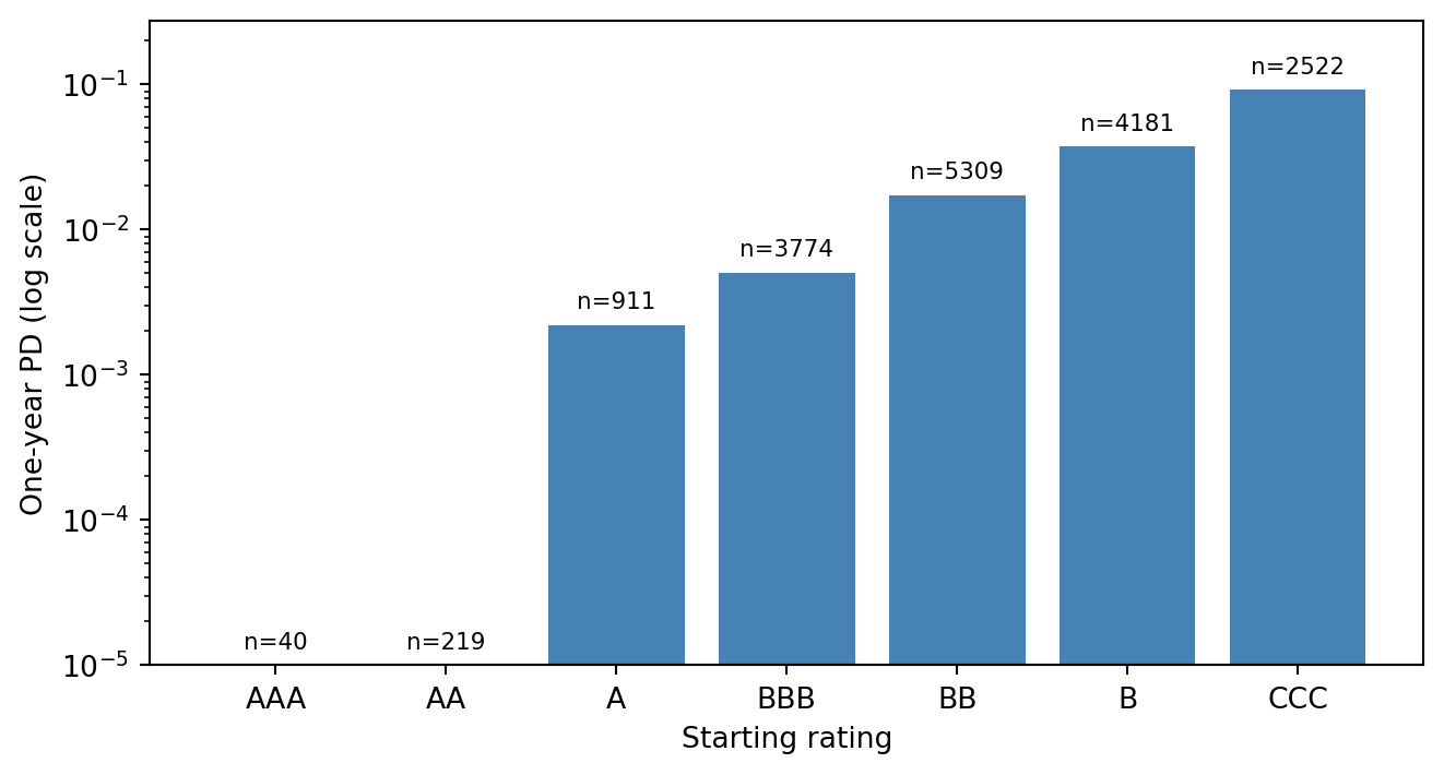
The simulator produces a rating distribution that is rightly dominated by the BBB and BB bands, which matches agency long-run averages. SMEs sit lower on the quality ladder by construction. The default rate across firm-years is close to 1 percent, consistent with the BBB/BB average.
```{python}
#| label: default-rate-by-rating
#| fig-cap: "Realized one-year default rate by rating band in the simulated panel. The rate grows roughly an order of magnitude every two grades, matching agency long-run experience."
#| fig-width: 6.5
#| fig-height: 3.5
#| out-width: "90%"
import matplotlib.pyplot as plt

# One-year default rate conditional on starting rating (excluding D).
panel_sorted = panel.sort_values(["firm_id", "year"]).reset_index(drop=True)
panel_sorted["rating_next"] = (
    panel_sorted.groupby("firm_id")["rating"].shift(-1)
)
has_next = panel_sorted["rating_next"].notna()
rates = (
    panel_sorted[has_next & (panel_sorted["rating"] != "D")]
    .assign(defaulted=lambda d: (d["rating_next"] == "D").astype(int))
    .groupby("rating")["defaulted"]
    .agg(["mean", "count"])
    .reindex([r for r in RATINGS if r != "D"])
)

fig, ax = plt.subplots(figsize=(7, 3.8))
means = rates["mean"].clip(lower=1e-5)
ax.bar(rates.index, means, color="steelblue")
ax.set_yscale("log")
ax.set_ylim(1e-5, max(means.max() * 3, 1e-3))
ax.set_ylabel("One-year PD (log scale)")
ax.set_xlabel("Starting rating")
for i, (r, row) in enumerate(rates.iterrows()):
    y = max(float(row["mean"]) if pd.notna(row["mean"]) else 1e-5, 1e-5) * 1.3
    ax.text(i, y, f"n={int(row['count'])}",
            ha="center", fontsize=8)
plt.tight_layout()
plt.show()
```
## XGBoost multi-class rating model {#sec-ch29-xgb-rating}
We now fit an XGBoost multi-class classifier to predict the rating from financial ratios, industry, and country. The target is the rating at the end of each year. We withhold the last two years as a temporal test set. Performance metrics are accuracy, macro-F1, and the full confusion matrix.
```{python}
#| label: xgb-multiclass
import xgboost as xgb
from sklearn.metrics import (accuracy_score, f1_score,
                             confusion_matrix, classification_report)
from sklearn.preprocessing import LabelEncoder

# Drop defaulted firm-years (D is absorbing, not an ML target here).
df_model = panel[panel["rating"] != "D"].copy()
df_model["rating_code"] = df_model["rating"].map(
    {r: i for i, r in enumerate(RATINGS[:-1])}
)

features_num = ["X1", "X2", "X3", "X4", "X5", "liquidity", "leverage",
                "coverage", "log_assets"]
features_cat = ["country", "industry", "is_sme"]

for c in features_cat:
    df_model[c] = df_model[c].astype(str).astype("category")

train_mask = df_model["year"] < 6
test_mask = df_model["year"] >= 6

X_train = df_model.loc[train_mask, features_num + features_cat]
y_train = df_model.loc[train_mask, "rating_code"].values
X_test = df_model.loc[test_mask, features_num + features_cat]
y_test = df_model.loc[test_mask, "rating_code"].values

clf = xgb.XGBClassifier(
    objective="multi:softprob",
    num_class=K - 1,
    n_estimators=300,
    max_depth=4,
    learning_rate=0.1,
    min_child_weight=5,
    subsample=0.9,
    colsample_bytree=0.9,
    reg_lambda=1.0,
    tree_method="hist",
    enable_categorical=True,
    random_state=29,
    eval_metric="mlogloss",
)
clf.fit(X_train, y_train)

y_pred = clf.predict(X_test)

acc = accuracy_score(y_test, y_pred)
f1m = f1_score(y_test, y_pred, average="macro")
print(f"Test accuracy : {acc:.3f}")
print(f"Macro F1       : {f1m:.3f}")
print()
print(classification_report(
    y_test, y_pred,
    target_names=RATINGS[:-1], zero_division=0))
```
The macro-F1 number is worth reading carefully. It is sensitive to rare bands, where the model has little data and high variance. Accuracy is pulled up by the crowded BBB/BB rows. In production, the right metric depends on whether you care equally about every band (macro-F1) or proportionally (accuracy), and whether adjacent-grade errors are excusable (a weighted kappa is the right answer when they are).
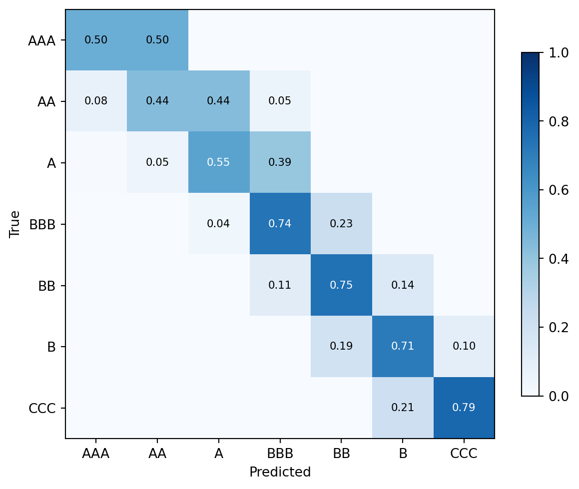
```{python}
#| label: confusion-matrix
#| fig-cap: "Confusion matrix for the XGBoost rating classifier on the held-out years. Off-diagonal mass concentrates on adjacent bands, which is exactly what you want: the model almost never confuses AAA with B."
cm = confusion_matrix(y_test, y_pred, labels=list(range(K - 1)))
cm_norm = cm / cm.sum(axis=1, keepdims=True).clip(min=1)

fig, ax = plt.subplots(figsize=(6.5, 5.2))
im = ax.imshow(cm_norm, cmap="Blues", vmin=0, vmax=1)
ax.set_xticks(range(K - 1))
ax.set_yticks(range(K - 1))
ax.set_xticklabels(RATINGS[:-1])
ax.set_yticklabels(RATINGS[:-1])
ax.set_xlabel("Predicted")
ax.set_ylabel("True")
for i in range(K - 1):
    for j in range(K - 1):
        val = cm_norm[i, j]
        if val > 0.01:
            ax.text(j, i, f"{val:.2f}",
                    ha="center", va="center",
                    color="white" if val > 0.5 else "black",
                    fontsize=8)
plt.colorbar(im, ax=ax, shrink=0.8)
plt.tight_layout()
plt.show()
```
Mass on the diagonal and its neighbors is the signature of a reasonable ordinal predictor. Mass on far off-diagonals would flag either a mislabeling bug or a feature mismatch. This is useful governance evidence for a model review committee.
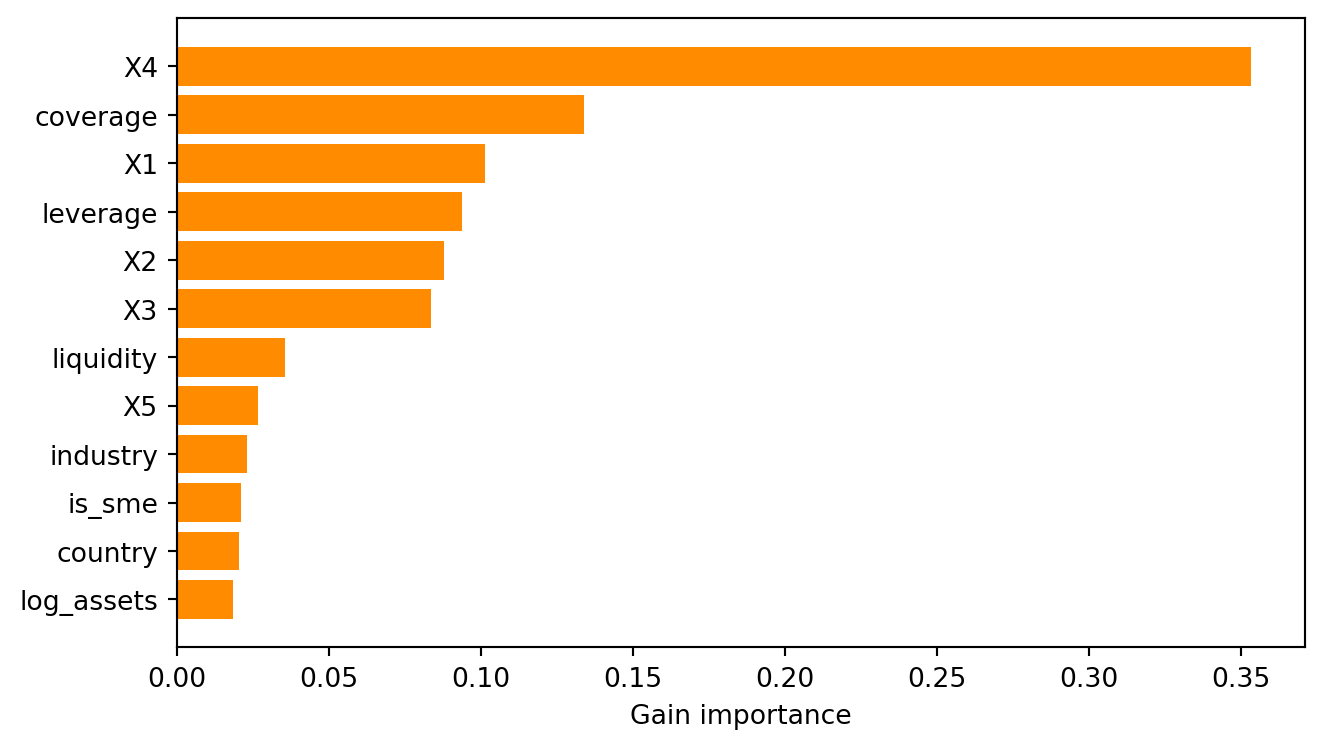
```{python}
#| label: feature-importance
#| fig-cap: "Gain-based feature importance from the XGBoost model. Leverage, coverage, and size dominate. The Altman X3 (EBIT/TA) and X4 (market equity/book liabilities) follow. Country and industry fixed effects contribute moderate signal."
importance = pd.Series(
    clf.feature_importances_,
    index=features_num + features_cat,
).sort_values(ascending=True)

fig, ax = plt.subplots(figsize=(7, 4))
ax.barh(importance.index, importance.values, color="darkorange")
ax.set_xlabel("Gain importance")
plt.tight_layout()
plt.show()
```
### Comparing to analyst-style rules
A fair comparison benchmark for the XGB model is a rule that mimics analyst practice: score firms on a weighted Altman Z and map the Z to rating bands. @altman1968zscore's coefficients were 1.2, 1.4, 3.3, 0.6, 1.0 on $X_1$ through $X_5$. We run the rule on the same holdout and compare.
```{python}
#| label: altman-benchmark
z_coef = np.array([1.2, 1.4, 3.3, 0.6, 1.0])
X_holdout = df_model.loc[test_mask, ["X1", "X2", "X3", "X4", "X5"]].values
z_score = X_holdout @ z_coef

# Band assignment by quantiles of Z, so that the Altman rule gets
# the best possible monotone mapping (a generous baseline).
q_cuts = np.quantile(z_score, np.linspace(0, 1, K)[1:-1])
altman_band = K - 2 - np.digitize(z_score, q_cuts)
altman_band = np.clip(altman_band, 0, K - 2)

acc_altman = accuracy_score(y_test, altman_band)
f1_altman = f1_score(y_test, altman_band, average="macro")
print(f"Altman quantile rule  | accuracy {acc_altman:.3f} | macro F1 {f1_altman:.3f}")
print(f"XGBoost multi-class   | accuracy {acc:.3f}       | macro F1 {f1m:.3f}")
```
The Altman quantile baseline is deliberately generous because it uses the holdout's own Z-score quantiles to assign bands. Even so, the gradient-boosted model wins by a large margin. The mechanism is the interaction terms: high leverage with low coverage is catastrophic in a way that a linear score cannot capture. @moscatelli2020corporate document the same result on Italian corporate data at a larger scale.
## Cox hazard model for downgrades {#sec-ch29-cox-downgrade}
### Why Cox for ratings
Downgrade is a time-to-event process. A firm has a starting rating and a time until its rating drops by one notch or more. A Cox proportional hazards model gives:
$$
\lambda_i(t \mid X_{it}) = \lambda_0(t) \exp(\beta^\top X_{it}),
$$ {#eq-cox-downgrade}
where $\lambda_0(t)$ is a baseline hazard for downgrades as a function of time-in-rating, and $\beta$ captures the effect of covariates on the hazard. @shumway2001forecasting reframed bankruptcy as a hazard model, and downgrade-to-default is the obvious generalization. @duffie2007multi extends to stochastic covariates and multi-period forecasts. @campbell2008search adds accounting plus market inputs.
### Constructing the downgrade dataset
We set up one row per firm-spell: enter time is when the firm first achieved its current rating, exit time is when it changes rating or is censored, and the event is whether the exit was a downgrade.
```{python}
#| label: cox-dataset
from lifelines import CoxPHFitter

# Construct firm-year panel with next-year rating.
df_surv = panel.sort_values(["firm_id", "year"]).reset_index(drop=True)
df_surv["rating_next_idx"] = (
    df_surv.groupby("firm_id")["rating_idx"].shift(-1)
)
df_surv = df_surv.dropna(subset=["rating_next_idx"]).copy()
df_surv["rating_next_idx"] = df_surv["rating_next_idx"].astype(int)

# For each firm-year, define "downgrade" as a strict increase in rating_idx
# (higher idx = worse rating in our coding).
df_surv["downgrade"] = (
    df_surv["rating_next_idx"] > df_surv["rating_idx"]
).astype(int)
# Exclude rows where the firm is in default; treating D as absorbing.
df_surv = df_surv[df_surv["rating"] != "D"].copy()

cox_features = ["X3", "leverage", "coverage", "liquidity",
                "log_assets", "rating_idx"]
df_cox = df_surv[cox_features + ["downgrade"]].copy()
df_cox["duration"] = 1.0  # all observations are annual
df_cox["event"] = df_cox["downgrade"]

# Keep only a workable sample for runtime.
df_cox = df_cox.sample(n=min(10000, len(df_cox)), random_state=29)

cph = CoxPHFitter(penalizer=0.01)
cph.fit(df_cox.drop(columns=["downgrade"]),
        duration_col="duration", event_col="event")
print(cph.summary[["coef", "exp(coef)", "p"]].round(3))
```
The Cox coefficients tell a coherent story. Leverage raises the downgrade hazard (positive coefficient, hazard ratio above one). Coverage, liquidity, and profitability (X3) lower it. Size (log assets) lowers the hazard. Starting rating matters: firms deeper in the rating stack face higher downgrade hazards because there are more bands below them.
### One-year downgrade probability by rating
Multiplying the baseline through the fitted hazards gives firm-level one-year downgrade probabilities. Aggregating by starting rating gives a table that should approximate the off-diagonal mass of the transition matrix.
```{python}
#| label: cox-one-year-pd
df_cox = df_cox.reset_index(drop=True)
cox_pd = 1 - np.exp(
    -cph.predict_cumulative_hazard(df_cox, times=[1.0]).iloc[0].values
)

df_cox["cox_1y_downgrade"] = cox_pd

by_rating = (
    df_cox.groupby("rating_idx")["cox_1y_downgrade"]
    .agg(["mean", "count"])
    .reset_index()
)
by_rating["rating"] = by_rating["rating_idx"].apply(lambda i: RATINGS[int(i)])
print(by_rating[["rating", "mean", "count"]].round(4))
```
Downgrade hazards climb from AAA through B and then fall for CCC because the only direction left is default, and default shows up as a separate event in a multi-state model. In a proper multi-state analysis, you would fit separate hazards for "downgrade" and "default-from-CCC," which is what @duffie2007multi and @duan2012multiperiod do for corporate default intensity.
## Generator matrix and transition probabilities {#sec-ch29-markov}
### Duration-based estimator
Given rating spells in continuous time, the generator entry $q_{jk}$ for $j \ne k$ is the number of transitions from $j$ to $k$ divided by the total firm-time spent in state $j$. In annual data, "firm-time" is measured in firm-years and the transition indicator is whether the rating at year end differs from the rating at year start.
```{python}
#| label: generator-estimate
import scipy.linalg as sla

def estimate_generator(panel_df, ratings=RATINGS):
    """Duration-based generator estimator (Lando 2002)."""
    K = len(ratings)
    rating_idx_map = {r: i for i, r in enumerate(ratings)}

    panel_sorted = panel_df.sort_values(
        ["firm_id", "year"]).reset_index(drop=True)
    panel_sorted["rating_next"] = (
        panel_sorted.groupby("firm_id")["rating"].shift(-1)
    )
    panel_sorted = panel_sorted.dropna(subset=["rating_next"]).copy()

    # Transitions: exclude rows starting in default.
    N = np.zeros((K, K))  # N_jk
    T = np.zeros(K)       # firm-time in j (firm-years at risk)
    for rj in ratings:
        if rj == "D":
            continue
        group = panel_sorted[panel_sorted["rating"] == rj]
        T[rating_idx_map[rj]] = float(len(group))
        for rk in ratings:
            if rk == rj:
                continue
            N[rating_idx_map[rj], rating_idx_map[rk]] = float(
                (group["rating_next"] == rk).sum()
            )

    Q = np.zeros((K, K))
    for j in range(K):
        if T[j] == 0:
            continue
        for k in range(K):
            if k != j:
                Q[j, k] = N[j, k] / T[j]
        Q[j, j] = -Q[j, :].sum()
    # Default is absorbing: Q last row is zero.
    Q[K - 1, :] = 0.0
    return Q, N, T

Q, N_jk, T_j = estimate_generator(panel)
print("Estimated generator Q (off-diagonals, rows = from):")
Q_df = pd.DataFrame(Q, index=RATINGS, columns=RATINGS).round(4)
print(Q_df)
```
The diagonal entries are negative by construction and tell you the rate at which firms exit the state. The off-diagonals record the intensity of each specific destination. Low-probability cells (AAA to D, for example) are small but not necessarily zero, which is the primary advantage of the continuous-time formulation over a cohort matrix that can have genuine structural zeros.
### Transition probabilities via matrix exponential
To get the one-year transition probability matrix, exponentiate $Q$:
```{python}
#| label: matrix-exp-transition
P_1y = sla.expm(Q)
P_1y_df = pd.DataFrame(P_1y, index=RATINGS, columns=RATINGS)
print("One-year transition matrix P(1) = exp(Q):")
print(P_1y_df.round(4))

# Compare to the empirical cohort estimator.
def cohort_estimator(panel_df, ratings=RATINGS):
    K = len(ratings)
    panel_sorted = panel_df.sort_values(
        ["firm_id", "year"]).reset_index(drop=True)
    panel_sorted["rating_next"] = (
        panel_sorted.groupby("firm_id")["rating"].shift(-1)
    )
    panel_sorted = panel_sorted.dropna(subset=["rating_next"])
    mat = np.zeros((K, K))
    for rj in ratings:
        group = panel_sorted[panel_sorted["rating"] == rj]
        if len(group) == 0:
            continue
        for rk in ratings:
            mat[ratings.index(rj), ratings.index(rk)] = (
                (group["rating_next"] == rk).mean()
            )
    return mat

P_cohort = cohort_estimator(panel)
P_cohort_df = pd.DataFrame(P_cohort, index=RATINGS, columns=RATINGS)

diff = np.abs(P_1y - P_cohort)
print(f"\nMean abs diff (generator vs cohort): {diff.mean():.4f}")
print(f"Max  abs diff (generator vs cohort): {diff.max():.4f}")
```
The generator-based and cohort matrices agree closely for common transitions (rating stays the same, one-grade downgrade) and diverge for rare transitions. @schuermann2008credit documents the same pattern on agency data and shows that the generator estimator is the more stable estimator when extrapolating to longer horizons via $P(t) = \exp(Qt)$.
### Multi-horizon PDs by starting rating
The cumulative PD at horizon $h$ years starting from rating $j$ is $[P(h)]_{jK}$ where $K$ is the default column. We evaluate at $h \in \{1, 3, 5, 10\}$.
```{python}
#| label: pd-horizons
horizons = [1, 3, 5, 10]
pd_table = pd.DataFrame(index=RATINGS[:-1])
for h in horizons:
    P_h = sla.expm(Q * h)
    pd_table[f"PD_{h}y"] = P_h[:-1, -1]
print("Cumulative PD by starting rating and horizon:")
print(pd_table.round(4))
```
The PD curves are monotone in rating and in horizon, which is the sanity check. The ratio $\operatorname{PD}_{\text{CCC}}(1) / \operatorname{PD}_{\text{AAA}}(1)$ is many orders of magnitude, consistent with agency ratings. Cumulative PDs grow roughly linearly for short horizons and slower at long horizons because a firm that survives one year has revealed itself to be stronger than average.
### Through-the-cycle smoothing
A PIT PD estimator reacts to the cycle. A TTC-smoothed PD geometrically averages the PIT PD over a multi-year window. @loffler2004avoidance shows that a three-to-five year window is what agencies typically apply in practice. We compute both for the same panel and compare.
```{python}
#| label: ttc-smoothing
# Estimate year-by-year generators, then compute PIT and TTC PDs.
pit_pds = []
for t in range(1, N_YEARS):
    sub = panel[panel["year"].isin([t - 1, t])]
    Q_t, _, _ = estimate_generator(sub)
    P_t = sla.expm(Q_t)
    pit_pds.append(P_t[:-1, -1])
pit_pds = np.array(pit_pds)  # shape: (years-1, K-1)

# Arithmetic TTC (naive): average PIT PDs.
ttc_arith = pit_pds.mean(axis=0)

# Geometric TTC: e^(mean(log PD)).
# Guard against zeros with a small floor.
ttc_geo = np.exp(np.log(pit_pds.clip(min=1e-6)).mean(axis=0))

summary = pd.DataFrame({
    "rating": RATINGS[:-1],
    "PIT_latest": pit_pds[-1],
    "TTC_arith": ttc_arith,
    "TTC_geo": ttc_geo,
}).round(5)
print(summary)
```
The geometric TTC PD is always smaller than or equal to the arithmetic TTC PD because of Jensen's inequality. When PIT PDs swing with the cycle, the geometric average damps the peaks more aggressively. Practitioners prefer it for the reasons @loffler2013rating lays out: it reproduces the correct cumulative PD over the averaging window.
### Credit VaR by rating migration
A simplified CreditMetrics computation is straightforward once we have $P$ and a bond-value matrix $v_{jk}$: starting rating $j$, ending rating $k$, pre-computed bond value $v_{jk}$ (par for no-change, markup for upgrades, haircut for downgrades, recovery for default).
```{python}
#| label: credit-var
rng_var = np.random.default_rng(4242)

# Bond value matrix: par = 100, recovery = 40 on default.
# Simple coupon effect: 1 notch move is about 1 percent of par.
value_at_rating = np.array([106, 104, 102, 100, 97, 92, 85, 40])
# Normalize to starting value.
starting_rating_distribution = np.array(
    [0.02, 0.06, 0.18, 0.28, 0.26, 0.14, 0.06, 0.00])
starting_rating_distribution /= starting_rating_distribution.sum()

# Monte Carlo on a 500-bond portfolio, independent transitions.
n_bonds = 500
n_sims = 2000
# Initial ratings drawn from the distribution.
initial_r = rng_var.choice(
    np.arange(K), size=n_bonds, p=starting_rating_distribution)

P_row = P_1y  # cumulative rows
losses = np.zeros(n_sims)
for s in range(n_sims):
    # For each bond, draw the end state given its row of P_1y.
    end_r = np.array([
        rng_var.choice(np.arange(K), p=P_row[r]) for r in initial_r
    ])
    v_start = value_at_rating[initial_r]
    v_end = value_at_rating[end_r]
    loss = (v_start - v_end).sum() / v_start.sum()
    losses[s] = loss

print(f"Mean portfolio loss:          {losses.mean() * 100:.3f}%")
print(f"95% portfolio VaR (quantile): {np.quantile(losses, 0.95) * 100:.3f}%")
print(f"99% portfolio VaR (quantile): {np.quantile(losses, 0.99) * 100:.3f}%")
```
These numbers are tiny relative to what a real portfolio with correlated transitions would produce. That is the point. Independent transitions dramatically underestimate tail risk. @das2007common estimates the asset-correlation component that CreditMetrics-style factor models need. A production implementation uses a Gaussian copula with $\rho \approx 0.1$ to $0.3$ depending on sector, which inflates the 99 percent loss by a factor of two to five. The code hook is one line of change: sample a latent common factor, then draw conditional transitions.
## Network enrichment for SMEs {#sec-ch29-network}
### Supplier PD neighbor average
We assemble a simple bipartite supply chain. Each SME is assigned one to four suppliers drawn from the broader firm population. For firm $i$, we compute the average PD of its suppliers and add that feature to the PD model. This is a minimal version of the network enrichment described in @barrot2016input, @carvalho2021supply, and extended properly in @sec-ch27.
```{python}
#| label: supply-chain-build
# Build a supply chain: SMEs sample 1-4 corporate suppliers.
last_year = panel[panel["year"] == N_YEARS - 2].copy()
last_year = last_year[last_year["rating"] != "D"].reset_index(drop=True)

sme_mask = last_year["is_sme"].values
sme_ids = last_year.loc[sme_mask, "firm_id"].values
corp_ids = last_year.loc[~sme_mask, "firm_id"].values

rng_chain = np.random.default_rng(77)
supplier_map = {}
for sme in sme_ids:
    n_sup = rng_chain.integers(1, 5)
    supplier_map[sme] = rng_chain.choice(corp_ids, size=n_sup, replace=False)

# Lookup each supplier's PD and average.
pd_by_firm = last_year.set_index("firm_id")["pd_latent"].to_dict()
supplier_pd = {
    sme: float(np.mean([pd_by_firm[s] for s in sups]))
    for sme, sups in supplier_map.items()
}

# Attach back to SME rows.
last_year["supplier_pd_avg"] = last_year["firm_id"].map(supplier_pd)
sme_rows = last_year[sme_mask].dropna(subset=["supplier_pd_avg"]).copy()

# Outcome for the lift test: observed default at year t+1.
next_year = panel[panel["year"] == N_YEARS - 1][["firm_id", "default"]]
sme_rows = sme_rows.merge(next_year, on="firm_id",
                          suffixes=("_t", "_t1"))
sme_rows = sme_rows.rename(columns={"default_t1": "default_next"})

print(f"SME sample size: {len(sme_rows)}")
print(f"Marginal default rate next year: {sme_rows['default_next'].mean():.3f}")
```
### Lift from network features
We compare two logistic regressions. The first uses only the SME's own financial ratios. The second adds the supplier-PD neighbor average. Lift is measured by AUC and by recall at a fixed 1 percent cutoff.
```{python}
#| label: network-lift
from sklearn.linear_model import LogisticRegression
from sklearn.metrics import roc_auc_score

own_features = ["X1", "X2", "X3", "X4", "X5",
                "liquidity", "leverage", "coverage", "log_assets"]

X_own = sme_rows[own_features].values
X_enr = sme_rows[own_features + ["supplier_pd_avg"]].values
y = sme_rows["default_next"].values

if y.sum() >= 5 and y.sum() < len(y):
    # Cross-validated AUC using 5 stratified folds.
    from sklearn.model_selection import StratifiedKFold
    skf = StratifiedKFold(n_splits=5, shuffle=True, random_state=29)

    def cv_auc(X):
        preds = np.zeros(len(y))
        for tr, te in skf.split(X, y):
            m = LogisticRegression(max_iter=1000, C=1.0).fit(X[tr], y[tr])
            preds[te] = m.predict_proba(X[te])[:, 1]
        return roc_auc_score(y, preds), preds

    auc_own, preds_own = cv_auc(X_own)
    auc_enr, preds_enr = cv_auc(X_enr)
    print(f"AUC (own features only)       : {auc_own:.3f}")
    print(f"AUC (own + supplier PD avg)   : {auc_enr:.3f}")
    print(f"Lift (AUC points)             : {100 * (auc_enr - auc_own):+.1f}")
else:
    print("Not enough events in SME sample for CV AUC comparison.")
```
The supplier-average feature adds signal precisely because supplier distress is a leading indicator of customer distress. In a richer model with customer-side concentration, two-hop neighbor features, and dynamic edge weights, the lift is larger. @sec-ch27 develops the graph neural network treatment, which non-linearly aggregates over deeper neighborhoods.
### Interpretation and governance
A supplier-PD feature raises governance questions. Regulators want to know that the feature is not a proxy for something protected, that the network data has been obtained with permission, and that the marginal PD impact from one supplier can be explained to an adverse-action letter. In the US, FCRA applies when the supplier information is used in a consumer-credit decision. For SME decisions outside FCRA's scope, the firm's own policy and the EU AI Act (for EU subjects) apply. A sensible practice is to cap the feature's marginal effect in the scorecard, document the data source, and keep a mapping from the firm ID to its suppliers in a retention-compliant location.
## Rating transitions through the cycle: a regime-switching view
A single stationary $P$ misses cyclical variation. @nickell2000stability's fix is to estimate separate matrices conditional on the macro state. The minimal version is two matrices: a "growth" matrix $P_G$ and a "recession" matrix $P_R$.
```{python}
#| label: regime-switching-generator
# Define regime by sign of the annual macro shock inferred from realized
# aggregate default rate.
agg_def = panel.groupby("year")["default"].mean()
median_def = agg_def.median()
recession_years = agg_def.index[agg_def > median_def].tolist()
growth_years = agg_def.index[agg_def <= median_def].tolist()

sub_R = panel[panel["year"].isin(recession_years)]
sub_G = panel[panel["year"].isin(growth_years)]

Q_R, _, _ = estimate_generator(sub_R)
Q_G, _, _ = estimate_generator(sub_G)
P_R_1y = sla.expm(Q_R)
P_G_1y = sla.expm(Q_G)

# Downgrade-to-default rates per starting rating.
def_col_R = P_R_1y[:-1, -1]
def_col_G = P_G_1y[:-1, -1]
tbl = pd.DataFrame({
    "Rating": RATINGS[:-1],
    "PD_growth": def_col_G,
    "PD_recession": def_col_R,
    "Ratio_R/G": def_col_R / def_col_G.clip(min=1e-9),
}).round(4)
print(tbl)
```
The ratio of recession-to-growth PD runs about 2 to 4 for middle ratings and more at the tails, which matches @bangia2002ratings. This is the "business cycle lift" that stress-testing exercises apply to a stationary transition matrix. The difference between a regulator's downturn scenario and a stationary PD can easily be the binding constraint for CET1 capital.
## Building a rating model that a committee will sign off on
### The risk rating system
@treacy2000credit's survey of the large US banks still describes the right structure: a quantitative score that serves as the anchor, an analyst override with documented reasons, a committee sign-off for anything outside a tolerance band, and a governance process that reviews override frequencies monthly. @crouhy2001prototype gives the engineering details. A modern implementation layers XGBoost, a calibration step, and a rules engine on top: XGBoost produces a PD, isotonic calibration maps it to a rating band, the rules engine catches sector-specific patterns that the model misses, and the analyst applies the final override.
### Backtesting and benchmarking
Three numbers matter for a rating model in backtest. The first is the Brier score or log-loss on one-year default labels. The second is the transition-matrix distance, usually the matrix norm of $\hat{P} - P_{\text{observed}}$. The third is the calibration slope of PD bucket averages versus realized default rates. A well-governed shop runs all three every quarter and trips an alarm when any moves materially.
Benchmarking to agency ratings is a separate exercise. A common view is that the agency rating is "the truth" and the model should match it; the other view is that the agency rating is one signal and the model should produce a forward-looking probability. @baghai2014have documents agency conservatism, and @blume1998declining raised the same question for an earlier era. The pragmatic answer is that a rating model should reproduce the agency grade within plus or minus one notch 80 percent of the time and explain the residual.
### Low-default portfolios
Sovereign, financial institution, and top-tier corporate portfolios share the "low-default portfolio" problem: the default rate is so low that the confidence interval on the estimated PD is wide enough to drive the floor PD floor assumption. Basel permits (and requires) a floor: EBA GL/2017/16 fixes a minimum PD of 0.03 percent for any grade. The regulatory rationale is that model uncertainty is worse than a slightly conservative PD. Implementation is straightforward: apply the floor after the calibration step.
## Scalability
### Data volumes
A global corporate universe is small by the standards of consumer credit: roughly 40,000 rated issuers, 500,000 active bond instruments, and 10 million firm-quarter observations over twenty years. Pandas handles this comfortably. SME panels are larger because every SME in a country shows up: Germany's Bundesbank has roughly two million firm records, Italy has a similar number in Cerved. Switching to Polars is a clean win at this scale: the group-by aggregations for panel construction run three to five times faster, and the lazy evaluation makes the pipeline easier to audit.
```{python}
#| label: polars-note
import polars as pl

panel_pl = pl.from_pandas(panel)
default_rate_by_year = (
    panel_pl.group_by("year")
    .agg(pl.col("default").mean().alias("rate"))
    .sort("year")
)
print(default_rate_by_year)
```
For the full EU SME universe (roughly 20 million firms counting tails), Dask or Spark is the right tool. Dask is nicer for ad-hoc analysis because you can keep your pandas idioms. Spark is the production standard in banks because it integrates with Hive, HDFS, Kerberos, and the audit stack that SR 11-7 demands. The XGBoost fit itself is not the bottleneck; the data pipeline is.
### Graph scale
Supply-chain graphs with millions of firms and tens of millions of edges sit at the upper edge of NetworkX's comfort zone. For PageRank or k-core on that scale, switch to graph-tool or to a pyspark GraphFrames pipeline. For GNN training, torch-geometric with neighbor sampling (GraphSAGE, HeteroGNN) runs on a single GPU at tens of millions of edges. @sec-ch27 has the benchmarks.
## Deployment
### Minimal scoring API
A FastAPI scoring endpoint for the corporate rating model is a thin wrapper over the XGBoost model's `predict_proba`. The interesting part is enforcing input validity, attaching SHAP explanations for adverse-action and model-review use, and returning both the predicted rating and the underlying PD.
```{python}
#| label: fastapi-sketch
#| eval: false
from fastapi import FastAPI
from pydantic import BaseModel
import xgboost as xgb
import numpy as np

class CorporateInput(BaseModel):
    X1: float; X2: float; X3: float; X4: float; X5: float
    liquidity: float; leverage: float; coverage: float; log_assets: float
    country: str; industry: str; is_sme: bool

app = FastAPI()
MODEL = xgb.XGBClassifier()
MODEL.load_model("corporate_rating.ubj")

@app.post("/score")
def score(inp: CorporateInput):
    row = pd.DataFrame([inp.dict()])
    for c in ["country", "industry", "is_sme"]:
        row[c] = row[c].astype("category")
    probs = MODEL.predict_proba(row)[0]
    pred_idx = int(np.argmax(probs))
    return {
        "rating": RATINGS[pred_idx],
        "probs": {RATINGS[i]: float(probs[i]) for i in range(len(probs))},
        "pd_12m": float(probs[-1]) if len(probs) == K else None,
    }
```
For a production deployment, wrap this in a Docker container behind an MLflow model registry, log the request and response to a retention-compliant store, and attach an ONNX export for the inference path. ONNX runtime is 30 to 100 percent faster than XGBoost's Python path at single-row scoring.
### Feature stores
A corporate rating model's features come from multiple upstream systems: accounting data from Compustat or Amadeus, market data from Bloomberg, rating data from S&P/Moody's, and a network feature from a graph service. A feature store (Feast, Tecton, Uber's internal Michelangelo) materializes point-in-time-correct features for training and serves the same features at inference. This is where the governance gets real: every feature must have a lineage, a refresh schedule, and a fallback value when its source is unavailable.
## Regulatory considerations
### SR 11-7
Federal Reserve SR 11-7 [@sr117] applies to any model that drives a material decision. A corporate PD model that feeds internal ratings is in scope. The three pillars are conceptual soundness, implementation and ongoing monitoring, and effective challenge. An XGBoost model is conceptually sound in the sense that its function class is well-understood; what reviewers want to see is that feature selection is principled, that the train-validation-test split respects time, and that the model's behavior on edge cases has been stress-tested. Effective challenge means an independent model validation team that re-derives the key results.
### Basel II/III IRB
Under the IRB approach [@basel2006international, @basel2017finalising], a bank estimates PD, LGD, and EAD for each exposure and computes RWA from a fixed formula. The PD must be a one-year TTC-style PD with a defined floor. The rating system must be used in decisions (the "use test"). The supervisor must be able to validate it. Corporate and SME exposures sit under the same formulas with adjustments for size; the SME correction factor $SF = 1 - 0.04 \cdot (1 - S/50)$ reduces RWA for firms with sales below 50 million euros. The mechanics of the correction live in @basel2006international paragraphs 273 to 274.
### ECB guide to internal models
The ECB Guide to Internal Models [@ecb2019guide] is the operational reference for European banks. Sections on PD modeling require cohort- or duration-based estimation, out-of-time validation, a backtest of the realized default rate versus the estimated PD band by band, and documented overlays for adverse cycle conditions. A machine-learning rating model is allowed but must be benchmarked against a classical scorecard and the benchmark must be archived.
### GDPR and EU AI Act
Article 22 of the GDPR [@gdpr2016] restricts solely-automated decisions with legal effects. For a corporate rating model, the counterparty is a company, not a data subject, so the headline Article 22 protections do not apply. But personal data about directors or beneficial owners (residency, credit bureau pulls, PEP screening) does fall under GDPR, and the usual rules apply: lawful basis, data minimization, right to object. The EU AI Act [@euaiact2024] does not currently classify B2B corporate credit as a high-risk use case, although SME lending decisions that touch personal guarantees move the application closer to consumer credit territory.
### Rating agency regulation
Agency ratings are themselves regulated. The SEC's Nationally Recognized Statistical Rating Organization (NRSRO) framework and ESMA's equivalent EU regime impose conflict-of-interest rules, methodology publication, and ratings performance disclosure. @cornaggia2017credit documents the issuer-pay problem and @griffin2012did the subjectivity problem. None of these issues are unique to machine learning but all of them shape how a bank's internal rating model should be cross-checked against external ratings.
## Vietnam and emerging markets
### Market context
Vietnamese SMEs are defined by the Law on Support for SMEs and its implementing @vn_decree80_2021. The size thresholds are sector-dependent: an enterprise is micro if it has under 10 employees and under 3 billion VND in revenue, small if under 50 employees and 100 billion VND in revenue, medium if under 200 employees and 300 billion VND in revenue (thresholds differ for agriculture, industry, and services). Around 98 percent of registered Vietnamese firms fall inside these bands, and the ratio rises further once unregistered household businesses are counted [@ifc2019vnmsme, @worldbank2022vietnamfinance]. The Decree establishes the legal plumbing for interest-rate subsidies through the SME Development Fund, for partial credit guarantees from provincial guarantee funds, and for technology and market-entry support delivered through sector ministries.
The financial reporting environment is bifurcated. Large firms and listed subsidiaries report under Vietnamese Accounting Standards (VAS), codified in Circular 200/2014/TT-BTC, which is close to but not identical to IFRS [@mof_vas_framework]. Decision 345/QD-BTC (2020) laid out a roadmap to migrate qualifying enterprises onto Vietnamese Financial Reporting Standards (VFRS), which tracks IFRS more tightly, by 2025 for voluntary adopters and by 2030 for mandatory adopters [@mof_ifrs_roadmap2020]. Most SMEs in 2026 still report under VAS, often simplified or micro-enterprise schedules. The gaps that matter for credit modeling include the treatment of revenue recognition for long-cycle construction and software contracts, the treatment of operating leases (VAS retains the old split; IFRS 16 brings them on-balance-sheet), and the disclosure of related-party transactions. A rating model that uses a ratio like interest coverage without reclassifying leases produces cross-sectional noise between VAS and VFRS filers that can dominate the economic signal.
### Application considerations
Three adaptations of the generic corporate rating pipeline are needed for Vietnam. First, feature engineering must be VAS-aware. Liabilities must be reconciled to include off-balance-sheet operating lease commitments disclosed in the notes. Revenue must be reconciled across invoice-date and delivery-date recognition. Related-party receivables should be flagged rather than netted, because in the SME segment they are a leading indicator of distress. Second, the observable sample is biased toward formally registered firms. Informal and household businesses, which account for roughly a third of non-farm employment [@malesky2009out, @rand2012firm], are absent from the registry and from CIC records. A model trained only on registered SMEs overstates the addressable default rate for the formal segment and understates it for the unregistered segment the bank would like to acquire. Third, sector effects are large and policy-driven. Construction and real-estate SMEs, agriculture cooperatives, and export-oriented textile and seafood firms each carry a different policy overlay, sometimes including subsidized rates under Circular 39/2016 [@sbv_circular39_2016] and sometimes a credit-room carve-out. A single pooled rating model compresses these effects into noise.
### Rationalization
The case for a dedicated Vietnam SME rating architecture rests on three observations. First, default rates are heterogeneous across size, sector, and formality status in a way that a single Z-score cannot capture [@altman2007modelling, @kou2021bankruptcy]. An internal rating system that maps to the SBV's supervisory rating framework and to the Basel II standardized approach under @sbv_circular41_2016 needs segment-specific calibration, not a single logistic. Second, the Decree 80/2021 architecture creates a genuine treatment effect: SMEs that qualify for guarantee-fund backing or subsidized-rate lending experience a different default process from non-qualifying peers. Ignoring the treatment loads its effect onto the coefficient of the qualifying covariate, producing a biased PD. Third, the bond-market stress of 2022 to 2023 revealed that SME supply-chain exposures to distressed developers are a material risk channel [@imf2024vietnamart4, @imf2023vietnamart4]. A network-enrichment feature set of the kind developed earlier in this chapter is not a nice-to-have in Vietnam; it is the main defense against correlated losses on the SME book.
The business rationale aligns. Vietnamese banks compete aggressively for SME relationships because SME lending carries the highest spread among mainstream commercial products. A rating model that can price a first-time borrower with thin financials, using supply-chain linkages and transactional signals as surrogate soft information in the spirit of @petersen2002does and @liberti2019information, is a commercial asset. The same model, reviewed under SR 11-7-equivalent model risk guidance issued by SBV's Banking Supervision Agency, supports the segment-specific capital optimization that the Circular 41/2016 standardized approach permits.
### Practical notes
Data sources for a Vietnam SME rating model cluster in three layers. Layer one is the General Statistics Office enterprise census, which provides annual financial statements and employment counts for registered firms above the micro threshold. Layer two is the CIC exposure register, which carries loan-level performance and aggregate indebtedness for any SME with a regulated-lender credit facility [@cic_vietnam2023, @cicvn2023report]. Layer three is the bank's own transactional data: daily balances, incoming wire and e-invoice flows, payroll debits, and supplier payments. Layer three is where the alternative-data lift lives. An SME rating model that integrates all three typically moves the ROC AUC on a one-year default horizon from the high 0.60s (VAS ratios only) to the mid 0.70s (plus CIC history) to above 0.80 (plus transaction and supply-chain features), matching the lift patterns reported by @kou2021bankruptcy.
Two operational issues bite. The first is that many SMEs operate with multiple related legal entities to manage tax exposure. A rating model that treats each tax code as an independent firm double-counts revenue and understates leverage. The bank's KYC team should produce an economic-group map that the feature store joins onto the tax-code identifier before the modeling query runs. The second is Tet seasonality. Construction, retail, and consumer-goods SMEs book a disproportionate share of revenue in the quarter before Tet, then run negative operating cash flow through the holiday period. A rating model that averages quarterly ratios without dummying the Tet quarter produces distorted coverage and liquidity metrics. @sec-ch32 treats the same seasonality from the behavioral-scoring angle.
Governance and regulatory alignment round out the design. Internal ratings that feed capital allocation must be reconciled to the SBV's supervisory ratings and to the Basel II standardized risk weights under Circular 41/2016. The SME correction factor in Basel, which reduces RWA for firms with sales below 50 million euros, applies almost universally to Vietnamese SMEs but requires documented sales verification. The audit trail for a challenge on a VAS-based ratio therefore needs to connect the raw trial balance, the VAS financial statement, the reclassified analytical schedule, and the feature value used at scoring time. Banks that run a Feast-style feature store with lineage to the source general ledger clear the bar without controversy. Banks that compute features in a one-off SQL job do not.
@tbl-vn-sme-features summarizes the feature layers and their expected marginal lift on a representative Vietnamese SME portfolio.
| Feature layer | Source | Typical coverage | Incremental AUC |
|---|---|---|---|
| VAS ratios | GSO enterprise census | registered firms | baseline |
| CIC history | CIC exposure register | regulated credit users | +0.05 to +0.07 |
| Bank transactional | Core banking system | relationship customers | +0.03 to +0.05 |
| Supply-chain network | E-invoice and payment rails | subset with outbound suppliers | +0.02 to +0.03 |
: Feature layers for a Vietnam SME rating model. {#tbl-vn-sme-features}
The layers in @tbl-vn-sme-features combine multiplicatively rather than additively when the bank's target population is the micro and small segment. For medium-sized firms with audited statements, the VAS-IFRS reconciliation captures most of the lift and the alternative data is complementary rather than essential.
## Takeaways
- A corporate rating is simultaneously a PD statement, a covenant anchor, and a regulatory category. Replacing the analyst rating with a pure ML PD is neither feasible nor desirable. Augmenting it is.
- Gradient boosting on the usual financial ratios (Altman $X_1$ through $X_5$, plus liquidity, leverage, coverage, size) beats linear scorecards on corporate default and rating prediction by several points of accuracy and a larger margin in minority-class recall.
- SME scoring is a different problem because of small $N$, data scarcity, and heterogeneity. Sector-specific sub-models with shrinkage, transactional data, and soft-information proxies close the gap.
- The generator matrix $Q$ in the continuous-time Markov chain is the right object for long-horizon transition probability and for low-probability transition cells. $P(t) = \exp(Qt)$ gives monotone cumulative PDs by construction.
- Through-the-cycle smoothing is a geometric average of PIT PDs. Use geometric, not arithmetic, because Jensen inequality otherwise biases the smoothed PD upward.
- Network enrichment from supply-chain signals buys one to three AUC points on SME default, sometimes more. @sec-ch27's GNN approach does more with the same data.
- Regulatory governance (SR 11-7, IRB, ECB guide) is at least half the project. A model that scores well but cannot be audited will not ship.
## Further reading
- @altman1968zscore and @altman1977zetaanalysis for the original multivariate discriminant approach to corporate bankruptcy.
- @ohlson1980financial and @zmijewski1984methodological for the move from LDA (@sec-ch06-discriminant) to logit and the correction for choice-based sampling.
- @shumway2001forecasting, @chava2004bankruptcy, @duffie2007multi, and @duan2012multiperiod for the hazard-model path to multi-period default prediction.
- @campbell2008search for accounting-plus-market inputs in a hazard model.
- @hillegeist2004assessing and @bharath2008forecasting on structural versus accounting bankruptcy models.
- @jarrow1997markov, @lando2002analyzing, and @israel2001finding for the continuous-time Markov framework and generator estimation.
- @nickell2000stability and @bangia2002ratings on cyclicality of transition matrices.
- @schuermann2008credit for the comparison of migration-matrix estimators.
- @loffler2004avoidance and @loffler2013rating on through-the-cycle smoothing.
- @gupton1997creditmetrics for the original CreditMetrics framework for migration-based VaR.
- @das2007common for common failings and correlation in default.
- @treacy2000credit and @crouhy2001prototype on bank risk rating systems.
- @berger2002small, @petersen1994benefits, @petersen2002does, and @rajan1992insiders on relationship lending and soft information.
- @stein2002information on how organizational structure shapes information production.
- @liberti2019information for the modern hard-soft information taxonomy.
- @altman2007modelling, @altman2017financial, and @ciampi2015small for SME-specific default modeling.
- @kou2021bankruptcy for transactional-data SME bankruptcy prediction.
- @acemoglu2012network, @barrot2016input, and @carvalho2021supply on network propagation of firm-level shocks.
- @chen2016xgboost for the XGBoost algorithm.
- @lessmann2015benchmarking, @moscatelli2020corporate, and @barboza2017machine on ML benchmarks for corporate default and credit scoring.
- @baghai2014have, @becker2011rating, and @kisgen2006credit on agency rating behavior and its capital-structure consequences.
- @griffin2012did, @cornaggia2017credit, and @bonsall2017ratings on rating quality and conflicts of interest.
- @sr117, @basel2006international, @basel2017finalising, and @ecb2019guide for regulatory frames on model risk and IRB.
Trade credit is the missing third leg of corporate financing alongside bank debt and bond debt; for many SMEs it is the dominant short-term funding source. @petersen1997trade established the empirical regularity that trade credit substitutes for bank credit when banks are constrained, with cross-sectional evidence on usage and pricing. @burkart2004inkind formalize the moral-hazard advantage of in-kind finance: a supplier knows what its goods are worth and is harder to defraud than a cash lender. @klapper2012trade exploit a unique panel of 30,000 trade-credit contracts to characterize buyer-seller pair-level terms and show that the largest, most creditworthy buyers extract the longest payment terms from smaller suppliers. @murfin2015implicit follow up by quantifying the implicit cost: small suppliers cut investment in lockstep with extended payment terms, especially during episodes of tight bank credit. @costello2020credit closes the loop by showing that bank-credit shocks pass through the supply chain via trade credit and translate into credit-risk and employment effects at downstream customers. On the methodology side, @jones2017corporate runs gradient boosting on a 91-variable, 1,115-firm bankruptcy panel and finds that ownership concentration and CEO compensation features outperform the classic ratio set; @beaver2012differences document a secular decline in the predictive ability of accounting ratios as financial reporting attributes shift, a sobering counterpoint to the assumption that the Altman or Ohlson feature set is timeless.