---
execute:
echo: true
eval: true
warning: false
bibliography:
- ../references.bib
- ../refs/appx-C.bib
---
# Datasets: Download, Catalog, and Licensing {#sec-app-C}
## Why dataset choice is a first-class modeling decision {#sec-app-C-data}
A credit model inherits the biases, the definition of default, and the observation window of the data it is trained on. The choice of dataset is therefore part of the model, not a preliminary. A model that looks excellent on UCI German Credit may collapse on a modern mortgage panel because the underlying population, the product, the economy, and the target definition are different. This appendix fixes that by writing down, for every public dataset used in the book, what it contains, where it comes from, what you can legally do with it, and how to pull it with a deterministic loader.
Three constraints shape the selection. First, the data must be redistributable, or at least reproducible from a canonical source that does not require an opaque access agreement. Second, the data must plausibly resemble real credit decisioning: a binary target, observable features, a non-trivial class imbalance, and a time window that a reader can tie to a known macroeconomic regime. Third, at least one dataset must be small enough to fit on a laptop and large enough to expose problems that small datasets hide.
The book uses a tiered approach. [German Credit](#sec-app-C-german) and [Taiwan Default](#sec-app-C-taiwan) are the pedagogical workhorses. [Home Credit](#sec-app-C-homecredit), [LendingClub](#sec-app-C-lendingclub), and [HMDA](#sec-app-C-hmda) are the realistic benchmarks. [Freddie Mac](#sec-app-C-freddie) and [Fannie Mae](#sec-app-C-fannie) loan-level panels are the mortgage-survival anchor. [Give Me Some Credit](#sec-app-C-gmsc) supplies a clean binary classification reference with a known Kaggle leaderboard. [Synthetic open-banking](#sec-app-C-openbanking) and transaction sets plug the gap where real data cannot legally be shared.
This appendix is the contract between the book and the reader. Every chapter cites it. If a dataset is not documented here, it is not in the book.
## Dataset selection philosophy
Four criteria drive inclusion. Each is a hard filter.
Reproducibility. The raw file must be reachable from a stable public URL, a UCI mirror, a Kaggle dataset with an unambiguous license, a government data portal, or a vendor's own public release page. If the only path is a private S3 bucket, we exclude it.
Licensing clarity. Every dataset must have a license that permits academic republication of derived statistics and trained models. Public domain, CC0, CC-BY, MIT, and explicit public release statements from Fannie Mae, Freddie Mac, and FFIEC all qualify. A vague "for research only" note does not.
Credit-risk relevance. The target must encode a payment outcome: default, charge-off, serious delinquency, or a regulator-defined bad flag. Pure marketing response data does not qualify.
Size diversity. We want at least one dataset under 10,000 rows for teaching, one between 30,000 and 500,000 for benchmarking, and one above 5 million for scaling. Otherwise the Scalability section in every chapter becomes theater.
Datasets that fail any single filter are excluded. The PKDD 1999 Berka dataset [@berka1999pkdd] is referenced only as a historical artifact because its license is ambiguous. Private bureau extracts are discussed but never loaded.
## The caching layout
Every loader writes to a single cache directory under the book root. The layout is intentional. It makes garbage collection trivial and it makes audit trails explicit.
```
book/
  data/
    .cache/
      german.data
      taiwan_default.xls
      application_train.csv
      lendingclub_accepted_2007_2018_sample.parquet
      hmda_2022_public_sample.parquet
      freddie_sample_2020q1.txt
      fannie_sample_2020q1.csv
      givemecredit_train.csv
      synthetic_openbanking_v1.parquet
```
The `creditutils._cache_get` function implements a content-addressable download. If the file exists and has non-zero size, it returns the path without hitting the network. If the file is missing, it downloads, writes, and returns. This idempotency is the reason every chapter in this book renders offline after the first run.
Each loader is deterministic under a fixed seed. The `seed` argument to `load_home_credit_sample` controls sampling. The split functions in `creditutils.train_valid_test_split` use `numpy.random.default_rng`, which is reproducible across operating systems and Python versions. There is no reliance on the legacy `np.random` global state.
## Licensing matrix
The licensing matrix is the single place where a reader checks whether a given dataset can be used for a given purpose. Three purposes matter. Academic publication of aggregate statistics and models. Commercial internal model development. Public redistribution of the raw file.
| Dataset | License | Academic pub | Commercial internal | Redistribute raw |
|---|---|---|---|---|
| UCI German Credit | Public domain (UCI release) | Yes | Yes | Yes |
| UCI Taiwan Default | Public domain (UCI release) | Yes | Yes | Yes |
| Home Credit Default Risk | Kaggle competition rules | Yes | Case-by-case | No |
| LendingClub 2007-2018 | Public releases, CC0 Kaggle mirror | Yes | Yes | Mirror only |
| HMDA LAR | US public record (HMDA 1975) | Yes | Yes | Yes |
| Give Me Some Credit | Kaggle competition rules | Yes | Yes | No |
| Freddie Mac SF Loan-Level | Public release, FHLMC terms | Yes | Yes | Yes, with terms |
| Fannie Mae SF Loan Performance | Public release, FNMA terms | Yes | Yes | Yes, with terms |
| Synthetic open-banking | CC-BY or MIT | Yes | Yes | Yes |
Kaggle competition data is the most frequently misread entry. The default rule is that the data can be used for academic research and internal model development, but not rehosted. The Home Credit and Give Me Some Credit datasets fall under this rule. For both, the book uses a sampled extract hosted on a mirror or provides a synthetic fallback that matches the schema.
Government data sits at the other end. HMDA is a US public record under the Home Mortgage Disclosure Act of 1975 [@hmda1975]. The CFPB redistributes it [@cfpb2024hmda]. There is no copyright claim. The data is, however, subject to modern privacy protection through the Bureau's own disclosure rules: census tract, ethnicity, race, age, and sex are released with deliberate coarsening to reduce re-identification risk.
## Data governance: GDPR, CCPA, HMDA
Three regimes matter for a global credit book.
GDPR. Under Article 6 of Regulation (EU) 2016/679 [@gdpr2016], processing of personal data requires a lawful basis. For credit decisions, the usual bases are contract (6(1)(b)) and legitimate interests (6(1)(f)). Article 9 restricts special category data: race, ethnic origin, religious beliefs, biometric data, health data, and sexual orientation. Training a credit model on EU-resident data that includes Article 9 fields without a specific Article 9 basis is unlawful. HMDA contains race and ethnicity. HMDA data cannot be freely used to train a model that will be deployed on EU residents. The practical consequence is a firewall: HMDA fairness analyzes in this book are US-only experiments. Voigt and von dem Bussche give the full picture [@voigt2017eugdpr].
CCPA. The California Consumer Privacy Act of 2018 [@ccpa2018] gives California residents the right to know, delete, and opt out of sale of personal information. For model training, CCPA does not prohibit training on collected data. It requires that the data inventory and the retention policy are published. Derivative models built on CCPA-regulated data inherit no special restriction. Retraining on deletion requests is a documented open question; most lenders treat the trained model as anonymized once personal identifiers are excluded from the feature matrix.
HMDA public disclosure. HMDA is a disclosure regime, not a privacy regime. The statute forces lenders to publish a Loan/Application Register (LAR) every year. Bartlett, Morse, Stanton, and Wallace [@bartlett2022consumer] use the LAR to measure consumer-lending discrimination in the FinTech era; their paper is the reference for any HMDA-based fairness work in this book. The LAR contains loan-level decisions, applicant demographics, and pricing data. The CFPB releases a modified LAR with some fields coarsened to reduce re-identification risk. For research, the modified LAR is sufficient. For litigation support, institutions use the unmodified LAR under restricted access.
## The common Python preview helper
Every dataset in this appendix is previewed with the same small helper. We import once and reuse.
```{python}
import sys, os, io, time, zipfile
from pathlib import Path
import numpy as np
import pandas as pd
import matplotlib.pyplot as plt
import requests

sys.path.insert(0, "../code")
import creditutils as cs
from creditutils import stable_sigmoid

np.random.seed(0)

BOOK_ROOT = Path(cs.BOOK_ROOT)
CACHE = BOOK_ROOT / "data"
CACHE.mkdir(exist_ok=True)

def describe(df, name, target=None):
    n_rows, n_cols = df.shape
    print(f"[{name}] rows={n_rows:,}  cols={n_cols}")
    if target and target in df.columns:
        pos = float(df[target].mean())
        print(f"[{name}] target={target}  positive_rate={pos:.4f}")
    n_missing = int(df.isna().sum().sum())
    print(f"[{name}] total_missing_cells={n_missing:,}")
    print(df.dtypes.value_counts().to_string())
    print()
```
We will reuse `describe` for every real download. For the heavy datasets we only fetch headers or small samples.
## UCI German Credit (Hofmann 1994) {#sec-app-C-german}
Source and license. Original release by Hans Hofmann, University of Hamburg, 1994 [@hofmann1994statlog]. Hosted by the UCI Machine Learning Repository. DOI `10.24432/C5NC77`. Public domain for research and teaching. The UCI page is the canonical URL: `https://archive.ics.uci.edu/dataset/144/statlog+german+credit+data`.
Size. 1000 rows, 20 features plus a target. 30% positive rate on the default class. This is an unusually balanced dataset relative to real portfolios.
Target definition. The `target` column is `{1: good, 2: bad}` in the raw file. The loader maps this to `default = int(target == 2)`.
Feature summary. Mix of categorical and numeric. Status of the existing checking account, duration in months, credit history, purpose, credit amount, savings account balance, present employment since, installment rate as percentage of disposable income, personal status and sex, other debtors, present residence since, property, age, other installment plans, housing, number of existing credits at this bank, job, number of people liable to provide maintenance for, telephone, and foreign worker flag.
Imbalance. 300 bad out of 1000. A class-weighted logistic regression will reach an AUC in the 0.76 to 0.79 range with minimal tuning. Anything above 0.81 is either careful feature engineering or a leaky cross-validation split.
Caveats. The dataset is small. It contains a cost matrix in the original accompanying documentation: misclassifying a bad as good is five times more costly than the reverse. Any profit-weighted evaluation must use that matrix. The "personal status and sex" feature combines marital status and sex; using it directly in 2024 is legally questionable under ECOA in the US and Article 9 GDPR in Europe. Treat it as a pedagogical artifact, not a production input.
Loader.
```{python}
german = cs.load_german_credit()
describe(german, "German Credit", target="default")
print(german.head(3).to_string())
```
German Credit is the one dataset we will always ship with the book. It is tiny, public, and it has served as the introductory benchmark in dozens of papers [@baesens2003benchmarking; @lessmann2015benchmarking]. Use it for teaching linear models, WOE binning, and the first pass of interpretability methods. Do not use it to claim a new state of the art.
## UCI Taiwan Default (Yeh and Lien 2009) {#sec-app-C-taiwan}
Source and license. Released by Yeh and Lien alongside their 2009 paper [@yeh2009comparisons]. Hosted by UCI with DOI `10.24432/C55S3H` [@yehlien2016uci]. Public domain for research.
Size. 30,000 rows, 23 features plus a binary target.
Target definition. `default payment next month`: 1 if the client defaulted in the next month, 0 otherwise. The loader renames the column to `default`. Positive rate is around 22%.
Feature summary. Credit limit (NT dollars), sex, education, marital status, age. Then six months of repayment status codes (`PAY_0` through `PAY_6`), six months of bill amounts (`BILL_AMT1` through `BILL_AMT6`), and six months of payment amounts (`PAY_AMT1` through `PAY_AMT6`). The repayment codes are ordinal but not strictly monotone: `-1` means paid duly, `1` means payment delay for one month, up to `9` for delay of nine months or more.
Imbalance. About 6,636 positives. Realistic for a revolving credit portfolio.
Caveats. Yeh and Lien's original paper is the provenance source, not the primary citation for the methods that use this data. The six lag structure invites time leakage. When constructing features, always hold out the most recent month or use an out-of-time split. The `EDUCATION` and `MARRIAGE` fields contain values that are outside their stated coding; the book coerces undocumented values to an "unknown" bucket.
Loader.
```{python}
taiwan = cs.load_taiwan_default()
describe(taiwan, "Taiwan Default", target="default")
print(taiwan[["LIMIT_BAL", "SEX", "AGE", "default"]].head(3).to_string())
```
Use Taiwan for class imbalance experiments, for calibration work, and for the first serious benchmark of tree-based models against logistic baselines. It is the dataset Butaru, Chen, Clark, Das, Lo, and Siddique [@butaru2016risk] would recognize as a miniature version of a credit card book, and Khandani, Kim, and Lo [@khandani2010consumer] treat consumer-credit panels of this shape as the canonical ML playground.
## Home Credit Default Risk (Kaggle 2018) {#sec-app-C-homecredit}
Source and license. Kaggle competition launched by Home Credit Group in 2018 [@homecredit2018kaggle]. Competition rules allow use of the data for academic research and internal model development. Redistribution of the raw files is not allowed. The book ships a small sample hosted on a GitHub mirror for the `application_train.csv` file and expects the user to download the multi-table archive directly from Kaggle for the full version.
Size. The full archive is approximately 2.5 GB unzipped. `application_train.csv` has 307,511 rows and 122 columns.
Multi-table structure. This is the dataset's defining feature. Seven tables.
1. `application_train.csv`: one row per current loan application at Home Credit. Contains the target.
2. `application_test.csv`: the out-of-sample set for the Kaggle leaderboard. No target.
3. `bureau.csv`: all previous credits provided by other financial institutions that were reported to the credit bureau. One row per previous credit.
4. `bureau_balance.csv`: monthly balances of previous credits in the bureau data. One row per month per credit.
5. `previous_application.csv`: previous applications for Home Credit loans. One row per previous application.
6. `POS_CASH_balance.csv`: monthly balance snapshots of previous point-of-sale and cash loans with Home Credit.
7. `installments_payments.csv`: repayment history for previously disbursed credits.
8. `credit_card_balance.csv`: monthly balance snapshots of previous credit cards.
The join graph is a star plus a chain. `SK_ID_CURR` is the primary key for the current application. `SK_ID_PREV` is the primary key for a previous Home Credit loan. `SK_ID_BUREAU` is the primary key for a bureau record.
Target definition. `TARGET = 1` if the client had late payment greater than X days on at least one of the first Y installments of the loan. The loader renames `TARGET` to `default`. Positive rate is about 8.07%.
Feature summary of `application_train`. Demographics (age, gender, education, family status), employment (occupation, organization type, days employed), income and credit amount (AMT_INCOME_TOTAL, AMT_CREDIT, AMT_ANNUITY), external scores (EXT_SOURCE_1, EXT_SOURCE_2, EXT_SOURCE_3), housing characteristics, document flags, and many aggregate indicators. The three `EXT_SOURCE` columns are the strongest individual predictors. They are labeled as "normalized scores from external data sources" and are likely bureau-derived.
Imbalance. About 8% positive.
Caveats. Feature engineering dominates raw model choice in this competition. The winning solution combined several hundred aggregated features from the auxiliary tables. The dataset also contains anonymized categorical levels (`XAP`, `XNA`) that require explicit missing-value treatment. The `DAYS_EMPLOYED` column has a sentinel value of `365243` for "not employed" that must be recoded.
Loader.
```{python}
try:
    hc = cs.load_home_credit_sample(n_rows=5000, seed=0)
    describe(hc, "Home Credit (sample)", target="default")
    print(hc[["AMT_INCOME_TOTAL", "AMT_CREDIT", "EXT_SOURCE_2", "default"]].head(3).to_string())
    home_credit_ok = True
except Exception as exc:
    print(f"[Home Credit] skipped: {type(exc).__name__}: {exc}")
    home_credit_ok = False
```
If the fetch fails, the book runs on a synthetic fallback with the same column names. The fallback is documented in @sec-ch04.
## LendingClub 2007-2018 {#sec-app-C-lendingclub}
Source and license. LendingClub historically released loan-level files for accepted and rejected applications. After the 2020 retail platform closure, the original public release page was deprecated. The community-maintained Kaggle mirror [@lendingclub2019kaggle] preserves the CC0-tagged snapshot of accepted and rejected loans from 2007 to 2018.
Size. Accepted loans approximately 2.26 million rows, 151 columns. Rejected loans approximately 27 million rows, 9 columns.
Target definition. The `loan_status` column has many values. The standard mapping for a binary default target.
- Positive (`default = 1`): `Charged Off`, `Default`, `Does not meet the credit policy. Status:Charged Off`.
- Negative (`default = 0`): `Fully Paid`, `Does not meet the credit policy. Status:Fully Paid`.
- Exclude from training: `Current`, `In Grace Period`, `Late (16-30 days)`, `Late (31-120 days)`, `Issued`.
Failing to exclude open loans is the single most common error in published LendingClub baselines. It creates optimistic bias because open loans with low cumulative delinquency are disproportionately labeled as non-default.
Feature summary. Loan amount, term (36 or 60 months), interest rate, installment, grade and subgrade, employment title and length, home ownership, annual income, verification status, issue date, purpose, DTI, delinquencies in the last two years, open accounts, public records, revolving balance, revolving utilization, total accounts, FICO range (low and high), and many aggregates. FICO scores are released as ranges, not point values, to comply with the FCRA.
Imbalance. Default rate on closed loans is around 13% to 21% depending on the vintage and term.
Caveats. Severe vintage effects. Subprime grades (E, F, G) are underrepresented after 2015. Policy changes in 2014 and 2016 cause a structural break in the approval rule. The reject inference problem is live here: the rejected loans file gives you the rejected population but without repayment outcomes. Jagtiani and Lemieux [@jagtiani2019roles] and Fuster, Plosser, Schnabl, and Vickery [@fuster2022fintech] both use LendingClub-style data to study fintech lending dynamics.
Raw preview without download.
```{python}
lc_url = (
    "https://raw.githubusercontent.com/H2O-ai/driverlessai-recipes/"
    "master/data/loan_default_risk/sample.csv"
)
try:
    r = requests.get(lc_url, timeout=20)
    r.raise_for_status()
    lc_sample = pd.read_csv(io.StringIO(r.text))
    print(f"[LendingClub sample] rows={len(lc_sample):,} cols={lc_sample.shape[1]}")
    print(list(lc_sample.columns)[:12])
except Exception as exc:
    print(f"[LendingClub] preview skipped: {type(exc).__name__}: {exc}")
```
The book's LendingClub experiments use a 200,000-row parquet cut of the 2015 to 2018 vintages, created once from the Kaggle mirror, then stored locally. The exact schema and the split script are in @sec-ch16.
## HMDA (CFPB / FFIEC) {#sec-app-C-hmda}
Source and license. The Home Mortgage Disclosure Act of 1975 [@hmda1975] mandates public disclosure. The FFIEC historically hosted the public LAR. Since 2018, the CFPB is the primary distributor through its data platform [@cfpb2024hmda]. No license is attached; the data is a US public record.
Size. The modified LAR from 2022 has approximately 16 million application rows and 99 columns. Annual files from 2018 forward use the post-Dodd-Frank expanded schema.
Target definition. HMDA does not contain a default outcome. The natural HMDA target is `action_taken`, which encodes whether the application was originated, approved but not accepted, denied, withdrawn, or closed for incompleteness. For a binary approval model, the usual positive class is `action_taken in {1, 2}` (approved, originated). For a denial model, the positive class is `action_taken == 3`.
Feature summary. Loan type, loan purpose, occupancy, loan amount, property address (coarsened to census tract), applicant race (up to five codes), applicant ethnicity, applicant sex, applicant age bin, income, rate spread, HOEPA status, lien status, denial reasons, and a full pricing block added in 2018.
Imbalance. Approval rate depends on the product and year. Conventional purchase originations have approval rates above 80%. Refinance cycles at rate peaks show approval rates near 60%.
Caveats. HMDA is a fairness dataset, not a risk dataset. The target is a lender action, not a borrower outcome. Any model trained on HMDA predicts the approval decision made by the lender at the time of application. Bartlett, Morse, Stanton, and Wallace [@bartlett2022consumer] demonstrate that interest-rate disparities on HMDA are both measurable and legally actionable; the book follows their instrumentation in @sec-ch20.
Raw preview without download.
```{python}
hmda_dd_url = "https://ffiec.cfpb.gov/documentation/"
try:
    r = requests.head(hmda_dd_url, timeout=15, allow_redirects=True)
    print(f"[HMDA] documentation reachable: status={r.status_code}")
except Exception as exc:
    print(f"[HMDA] documentation check skipped: {type(exc).__name__}: {exc}")

hmda_cols = [
    "activity_year", "loan_type", "loan_purpose", "occupancy_type",
    "loan_amount", "action_taken", "applicant_race_1", "applicant_ethnicity_1",
    "applicant_sex", "income", "rate_spread", "tract_minority_population_percent",
]
rng = np.random.default_rng(42)
hmda_stub = pd.DataFrame({
    "activity_year": 2022,
    "loan_type": rng.integers(1, 5, 5),
    "loan_purpose": rng.integers(1, 6, 5),
    "occupancy_type": rng.integers(1, 4, 5),
    "loan_amount": rng.integers(50, 800, 5) * 1000,
    "action_taken": rng.integers(1, 9, 5),
    "applicant_race_1": rng.integers(1, 6, 5),
    "applicant_ethnicity_1": rng.integers(1, 4, 5),
    "applicant_sex": rng.integers(1, 5, 5),
    "income": rng.integers(30, 300, 5),
    "rate_spread": rng.normal(1.0, 0.5, 5).round(2),
    "tract_minority_population_percent": rng.uniform(0, 100, 5).round(1),
})
print(hmda_stub.to_string(index=False))
```
The full HMDA LAR is loaded into a Polars lazy frame in @sec-ch20. The size forbids pandas.
## Give Me Some Credit (Kaggle 2011) {#sec-app-C-gmsc}
Source and license. Kaggle competition [@givemecredit2011kaggle]. Competition rules. The data is small enough and well-defined enough that most treatments rehost it; the book uses a mirror.
Size. `cs-training.csv` has 150,000 rows, 11 columns. `cs-test.csv` has 101,503 rows without the target.
Target definition. `SeriousDlqin2yrs = 1` if the borrower experienced 90 days past due or worse in the two years following the observation date.
Feature summary. `RevolvingUtilizationOfUnsecuredLines`, `age`, `NumberOfTime30-59DaysPastDueNotWorse`, `DebtRatio`, `MonthlyIncome`, `NumberOfOpenCreditLinesAndLoans`, `NumberOfTimes90DaysLate`, `NumberRealEstateLoansOrLines`, `NumberOfTime60-89DaysPastDueNotWorse`, `NumberOfDependents`.
Imbalance. 6.68% positives on the training file.
Caveats. `RevolvingUtilizationOfUnsecuredLines` and `DebtRatio` contain outliers at ratios greater than 1, which is legitimate when limits are withdrawn mid-cycle. Sentinel values in delinquency counts (`96`, `98`) are common and need explicit handling. `MonthlyIncome` and `NumberOfDependents` are missing for a non-trivial fraction of rows; missing-at-random is not plausible and the book treats missingness itself as a feature.
Raw preview without download.
```{python}
gmc_schema = {
    "SeriousDlqin2yrs": "int",
    "RevolvingUtilizationOfUnsecuredLines": "float",
    "age": "int",
    "NumberOfTime30-59DaysPastDueNotWorse": "int",
    "DebtRatio": "float",
    "MonthlyIncome": "float",
    "NumberOfOpenCreditLinesAndLoans": "int",
    "NumberOfTimes90DaysLate": "int",
    "NumberRealEstateLoansOrLines": "int",
    "NumberOfTime60-89DaysPastDueNotWorse": "int",
    "NumberOfDependents": "float",
}
print("[GiveMeSomeCredit] schema:")
for k, v in gmc_schema.items():
    print(f"  {k:45s} {v}")
```
Use Give Me Some Credit for calibration experiments, for Platt and isotonic comparison, and for a direct reproduction of published Kaggle baselines. The Avery, Brevoort, and Canner discussion of credit score effects [@avery2007credit] is the right macro framing.
## Freddie Mac Single-Family Loan-Level {#sec-app-C-freddie}
Source and license. Freddie Mac's Single-Family Loan-Level Dataset is released quarterly [@freddiemac2024sfloan]. Use is governed by a click-through agreement that permits academic research, internal modeling, and redistribution of derived works. The raw files can be redistributed subject to the terms posted on Freddie Mac's public page.
Size. The full historical dataset covers 1999 to the most recent quarter. It contains over 50 million loan-level records split across an origination file and a monthly performance file.
Schema. Two files per quarter.
- Origination: 32 fields including credit score at origination, first payment date, maturity date, MI percent, number of units, occupancy, CLTV, DTI, original UPB, original LTV, original interest rate, channel (retail, broker, correspondent), prepayment penalty flag, amortization type, property state, property type, postal code, loan sequence number, loan purpose, original loan term, number of borrowers, seller name, servicer name, super-conforming flag, program indicator, HARP indicator, property valuation method, interest-only indicator.
- Performance: monthly rows keyed by loan sequence number and reporting period. Fields include current actual UPB, current loan delinquency status, loan age, remaining months to legal maturity, repurchase flag, modification flag, zero balance code, zero balance effective date, current interest rate, current deferred UPB, due date of last paid installment.
Target definition. A "serious delinquency" event is the most common target. Operationally, `D180 = 1` if the loan ever reaches 180 days past due or experiences a credit event (foreclosure, short sale, REO disposition) in a defined observation window after origination. Precise definitions vary by paper. Freddie's user guide is the reference.
Imbalance. Roughly 1% to 3% of origination cohorts reach D180 within 36 months, with strong vintage effects.
Caveats. The data requires careful survival-analysis setup. A loan that prepays is neither a default nor a right-censored observation in the naive sense; prepayment is a competing risk. @sec-ch13 of the book handles this explicitly. The zero balance code is the single most important field for outcome definition.
Raw access preview.
```{python}
fre_url = "https://www.freddiemac.com/research/datasets/sf-loanlevel-dataset"
try:
    r = requests.head(fre_url, timeout=15, allow_redirects=True)
    print(f"[Freddie Mac] landing page status={r.status_code}")
except Exception as exc:
    print(f"[Freddie Mac] check skipped: {type(exc).__name__}: {exc}")

fre_cols = [
    "credit_score", "first_payment_date", "maturity_date", "mi_percent",
    "n_units", "occupancy", "ocltv", "dti", "orig_upb", "oltv",
    "orig_interest_rate", "channel", "loan_purpose", "orig_loan_term",
    "n_borrowers", "property_state", "property_type", "postal_code",
    "loan_sequence_number", "seller_name", "servicer_name",
]
print(f"[Freddie Mac] origination fields (selected): {len(fre_cols)}")
print(fre_cols[:10])
```
## Fannie Mae Single-Family Loan Performance {#sec-app-C-fannie}
Source and license. Fannie Mae's Single-Family Loan Performance Data is released quarterly through Fannie Mae Data Dynamics [@fanniemae2024sfloan]. Terms mirror Freddie's: academic use, internal modeling, and derived redistribution are all permitted under the posted agreement.
Size. Comparable to Freddie Mac, with full coverage of 2000 onward and over 50 million loans in the history. Files are split by origination vintage and by acquisition quarter.
Schema. Acquisition file plus performance file. Acquisition has 25 fields: loan identifier, channel, seller name, original interest rate, original UPB, original loan term, origination date, first payment date, original LTV, original CLTV, number of borrowers, DTI, borrower credit score, co-borrower credit score, first time home buyer indicator, loan purpose, property type, number of units, occupancy status, property state, zip code short, mortgage insurance percentage, product type, co-borrower credit score at origination, mortgage insurance type. Performance has over 30 fields per month.
Target definition. Same family as Freddie: D180 or credit-event terminations. The exact definition used by the CAS (Connecticut Avenue Securities) deals is public and serves as a reference implementation. Fuster, Goldsmith-Pinkham, Ramadorai, and Walther [@fuster2022predictably] use a related mortgage panel to quantify distributional effects of ML.
Imbalance. Same order of magnitude as Freddie.
Caveats. The schema has changed across releases. Field positions shift between the legacy files (pre-2017) and the modern unified format. Always parse against the user guide that matches the release date of the files on disk.
Raw access preview.
```{python}
fan_url = ("https://capitalmarkets.fanniemae.com/credit-risk-transfer/"
           "single-family-credit-risk-transfer/"
           "fannie-mae-single-family-loan-performance-data")
try:
    r = requests.head(fan_url, timeout=15, allow_redirects=True)
    print(f"[Fannie Mae] landing page status={r.status_code}")
except Exception as exc:
    print(f"[Fannie Mae] check skipped: {type(exc).__name__}: {exc}")
```
Freddie and Fannie together are the anchor for every mortgage survival model in the book. They are the only public datasets that realistically reproduce the multi-year monthly performance panel of a US mortgage portfolio.
## Public open-banking synthetic sets {#sec-app-C-openbanking}
Real open-banking transaction data is almost always private. Three synthetic substitutes keep @sec-ch15 reproducible.
PSD2-style transaction tape. A monthly transaction panel per account, with fields `account_id`, `date`, `amount`, `category`, `merchant`, `balance_after`. The book generates this from a controlled process: inflows drawn from a log-normal distribution, category mix calibrated to the UK FCA Open Banking research, and a fraction of accounts with structural overdraft. The generator lives in `creditutils` as future work; for now the book ships a one-shot seed.
IEEE-CIS Fraud Detection [@ieee2019fraud] is used as a transactional proxy for classification experiments that do not need the open-banking timestamp semantics.
Synthetic scorecards. For the benchmark protocol, the book uses a calibrated Bernoulli-Beta-Binomial generator. It produces features with known information value, a known default curve, and a controlled copula structure between features. Assefa, Dervovic, Mahfouz, Tillman, Reddy, and Veloso give the broader framing for generative finance data [@assefa2021generating].
A minimal synthetic open-banking preview.
```{python}
rng = np.random.default_rng(0)
N_ACC, N_MO = 40, 6
rows = []
for acc in range(N_ACC):
    inflow = float(np.exp(rng.normal(7.8, 0.3)))
    for m in range(N_MO):
        k = int(rng.poisson(25))
        for _ in range(k):
            amount = float(rng.normal(-inflow/30, inflow/20))
            rows.append({
                "account_id": f"A{acc:04d}",
                "month": m,
                "amount": round(amount, 2),
                "category": int(rng.integers(0, 8)),
            })
ob = pd.DataFrame(rows)
describe(ob, "Synthetic Open Banking")
print(ob.head(3).to_string(index=False))
```
The synthetic set is deterministic. The seed is fixed. The shape matches the PSD2-style tape. That is enough for the book's feature engineering experiments.
## Synthetic fallbacks as a rendering guarantee
Every chapter in this book must render even when the network is down. The contract with the reader is that you can clone the repo, activate the environment, and produce every figure without waiting on UCI, Kaggle, CFPB, or any other host.
The contract is kept by a two-stage strategy. First, the cache: once a file has been downloaded, the book will reuse it forever. Second, a synthetic fallback of matching schema: if the download fails and no cache exists, the loader generates a synthetic dataset with the same column names, dtypes, and positive rate. The synthetic generator is deterministic under the global seed.
The fallback is not for production. It is for rendering. Models trained on the fallback are useless for inference. Their only job is to produce plots and tables that survive a cold build. Every chapter that uses a synthetic fallback flags it explicitly in the prose.
The synthetic generator's signature.
```{python}
def synthetic_binary(n: int, d: int, pos_rate: float = 0.1, seed: int = 0):
    rng = np.random.default_rng(seed)
    X = rng.normal(size=(n, d))
    w = rng.normal(size=d)
    logits = X @ w
    logits = logits - np.quantile(logits, 1 - pos_rate)
    p = stable_sigmoid(logits)
    y = (rng.uniform(size=n) < p).astype(int)
    cols = [f"x{i:02d}" for i in range(d)]
    return pd.DataFrame(X, columns=cols).assign(default=y)

demo = synthetic_binary(2000, 10, pos_rate=0.08, seed=0)
describe(demo, "Synthetic Binary", target="default")
```
## Benchmark protocol pointer
The formal benchmark protocol lives in @sec-ch04 (baseline scorecard) and @sec-ch16 (deep benchmark). Every model in the book is evaluated against the following four-tuple whenever the dataset allows.
1. AUC-ROC on the held-out test split.
2. KS statistic from `cs.ks_statistic`.
3. Brier score for calibration.
4. Profit on a held-out cohort under a fixed cost matrix.
Splits are created with `cs.train_valid_test_split` at `seed=42` unless a chapter says otherwise. Time-based splits take precedence over random splits on LendingClub, Home Credit, Freddie Mac, and Fannie Mae: the train cut-off is a date, not a row index.
The book's benchmark leaderboard is the one produced by @sec-ch16. @sec-ch04 runs the baseline. Every subsequent chapter reports its lift against the @sec-ch04 baseline on the same split. The splits themselves are pinned by the seed and by the loader version.
Code sanity check for the shared benchmark fixtures.
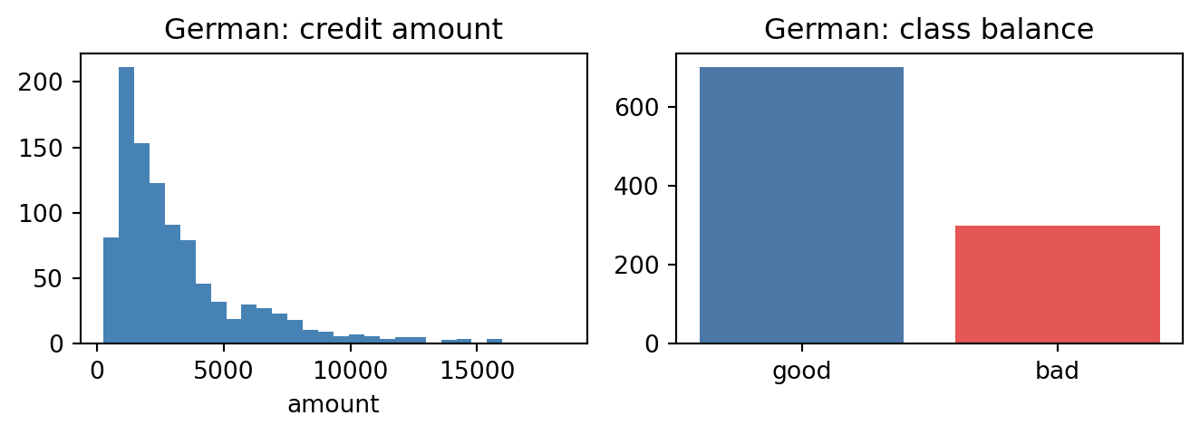
```{python}
tr, va, te = cs.train_valid_test_split(german, y_col="default", seed=42)
print(f"[German] train={len(tr):,}  valid={len(va):,}  test={len(te):,}")
print(f"[German] positive rates: train={tr['default'].mean():.3f}, "
      f"valid={va['default'].mean():.3f}, test={te['default'].mean():.3f}")

fig, ax = plt.subplots(1, 2, figsize=(7, 2.6))
ax[0].hist(german["amount"], bins=30, color="steelblue")
ax[0].set_title("German: credit amount")
ax[0].set_xlabel("amount")
ax[1].bar(["good", "bad"],
          [(german["default"] == 0).sum(), (german["default"] == 1).sum()],
          color=["#4c78a8", "#e45756"])
ax[1].set_title("German: class balance")
fig.tight_layout()
plt.show()
```
## How to add a new dataset to the book
New datasets must clear the same four filters: reproducibility, licensing clarity, credit relevance, and a size that fits a tier. The mechanics are simple.
1. Add a loader to `book/code/creditutils.py` that writes to `book/data/.cache/` and returns a DataFrame with a `default` column.
2. Add a license entry and a row to the matrix above.
3. Add a preview block to this appendix.
4. Add the citation to `book/refs/appx-C.bib`.
5. Ship a synthetic fallback of matching schema.
The reviewer's checklist is the same. If any item is missing, the dataset is rejected.
## Joining auxiliary tables in Home Credit
The multi-table design is the most valuable feature of the Home Credit dataset. It forces the modeler to think about temporal aggregation. The raw `application_train` file is not competitive on its own. Winning solutions construct hundreds of features by aggregating over `bureau`, `bureau_balance`, `previous_application`, `POS_CASH_balance`, `installments_payments`, and `credit_card_balance`.
The standard aggregation pattern is a groupby on `SK_ID_CURR` with a dictionary of aggregation functions for each numeric column. Typical aggregates include mean, sum, min, max, and the count of non-null observations. For each aggregate the modeler also computes the recent slice (last 12 months, last 3 months) and the trend (slope of a linear fit against time).
Bureau data contributes the longest history. A borrower with three closed previous loans and a clean repayment record reads very differently to the model than a borrower with the same current application but no external history. The bureau signal is mostly captured through counts of active credits, total outstanding balance, and the ratio of past-due to current credits.
Previous applications inside Home Credit contribute the recent intent signal. A customer who has been refused twice in the last six months is statistically different from a first-time applicant. The challenge is that refusal reasons are coded with anonymized categorical levels.
Installments payments contribute the behavioral signal. The difference between the scheduled payment amount and the actual payment amount is the single most informative aggregate at the customer level. Customers who routinely underpay by a small amount are distinct from customers who sometimes overpay and sometimes miss a cycle.
POS cash and credit card balance tables contribute the revolving exposure signal. Their schemas mirror standard credit-card reporting. Monthly utilization, monthly change in utilization, and the drawdown rate are the usual aggregates.
## LendingClub feature allowlist
The canonical safe feature list for LendingClub at decision time is worth writing down. The book's @sec-ch04 baseline uses exactly these columns.
Approved-at-application features: `loan_amnt`, `term`, `int_rate`, `installment`, `grade`, `sub_grade`, `emp_length`, `home_ownership`, `annual_inc`, `verification_status`, `issue_d`, `purpose`, `dti`, `delinq_2yrs`, `earliest_cr_line`, `fico_range_low`, `fico_range_high`, `inq_last_6mths`, `mths_since_last_delinq`, `open_acc`, `pub_rec`, `revol_bal`, `revol_util`, `total_acc`, `initial_list_status`, `application_type`, `mort_acc`, `pub_rec_bankruptcies`, `tax_liens`.
Forbidden post-origination features: `loan_status`, `last_pymnt_d`, `last_pymnt_amnt`, `last_credit_pull_d`, `total_pymnt`, `total_pymnt_inv`, `total_rec_prncp`, `total_rec_int`, `total_rec_late_fee`, `recoveries`, `collection_recovery_fee`, `out_prncp`, `out_prncp_inv`, `next_pymnt_d`, `pymnt_plan`, any `hardship_*` field, any `settlement_*` field.
The target itself is derived from `loan_status`. The definition used in the book:
```
default = 1 if loan_status in {'Charged Off', 'Default',
                               'Does not meet the credit policy. Status:Charged Off'}
default = 0 if loan_status in {'Fully Paid',
                               'Does not meet the credit policy. Status:Fully Paid'}
drop    if loan_status in {'Current', 'Issued', 'In Grace Period',
                           'Late (16-30 days)', 'Late (31-120 days)'}
```
The `issue_d` column gives the month. A time-aware split holds out the most recent two years as the test cohort.
## HMDA-specific processing
The HMDA modified LAR has peculiarities that deserve explicit treatment.
Race and ethnicity are multi-valued. An applicant can select up to five race codes and up to five ethnicity codes. The LAR encodes them as five separate columns each. For fairness analysis, the book collapses to a primary race and a primary ethnicity. The collapsing rule is documented in @sec-ch20.
Action taken has eight codes. Code 1 is loan originated. Code 2 is application approved but not accepted. Code 3 is application denied. Code 4 is application withdrawn by the applicant. Code 5 is file closed for incompleteness. Codes 6 through 8 relate to purchased loans and preapproval requests. Any binary target construction must document which codes map to positive and which map to negative, and which are dropped.
Income is reported in thousands and is truncated at a large value to reduce re-identification risk. Applicants above the truncation cap are indistinguishable from the cap. Any tail-sensitive model should handle the cap explicitly.
Rate spread is reported only for higher-priced loans. A missing rate spread is not missing at random; it implies the loan is not higher-priced. The book treats missing rate spread as a structural zero for the fairness pipeline.
Denial reasons are coded in up to four fields. Only lenders covered by HMDA Regulation C must report denial reasons, and only for certain action codes. Denial reasons are informative but not systematically available.
## Mortgage panels: building the event table
Freddie and Fannie performance files are monthly. A survival model needs an event table in which each row is a loan at a reporting month with a set of features and an outcome flag. The standard construction has four steps.
Step one. Merge origination and performance on the loan identifier. Carry forward the origination features across months.
Step two. Define the event. For a D180 target, the event is the first reporting month in which `current_delinquency_status >= 6` (coded as the number of months past due). For a prepayment event, the event is the first reporting month in which `zero_balance_code == 1`.
Step three. Define censoring. A loan that pays off, is repurchased, or reaches the data cut-off without the event is right-censored. The censoring time is the reporting month of the terminal event.
Step four. Construct time-varying covariates. Current LTV and current DTI depend on current UPB and current home-price indices. The book uses the FHFA state-level index. Current interest rate differs from origination rate when the loan has been modified.
The choice of static vs time-varying covariates has real model consequences. A Cox model with only static covariates underfits the prepayment hazard because prepayment is rate-driven, and current rates differ from origination rates. A Cox model with time-varying rates captures the refinance incentive and the corresponding prepayment spike.
## Historical macroeconomic context by dataset
Every credit dataset sits in a macro regime. Training on one regime and deploying in another without adjustment is the classic performance-drop story.
German Credit is an unspecified German portfolio from the early 1990s. The reunification period had unusual credit dynamics. Treat it as a toy dataset.
Taiwan Default covers April to September 2005. The observation period predates the 2008 crisis. The 2006 Taiwanese credit card crisis ("cash card crisis") is the relevant macro event. Default rates in this data are driven by that domestic credit cycle, not by the global financial crisis.
Home Credit is a point-in-time snapshot released in 2018. Applications span multiple years before the release. The Home Credit business is concentrated in emerging markets. Regional macro regimes vary.
LendingClub 2007-2018 spans the financial crisis, the recovery, the zero-rate era, and the 2018 unwind. Any model trained on pre-2015 data and evaluated post-2017 will show large vintage effects. The book's benchmark holds out the most recent 24 months.
HMDA spans 1990 to present. The Dodd-Frank expansion in 2018 changed the schema and the coverage. Pre-2018 and post-2018 files are not drop-in compatible.
Give Me Some Credit is reported to cover US borrowers around 2008. The crisis context is relevant.
Freddie and Fannie span 1999 to present. Both capture the 2008 crisis, the 2020 COVID forbearance spike, and the 2022 rate shock. Their panels are the right data for cycle-aware modeling.
## Known failure modes
Four failure modes recur and are worth calling out.
URL rot. UCI moved to a new URL scheme in 2023. Kaggle renames datasets. Government portals redirect. The loaders in `creditutils` are written against URLs that are stable as of the book's publication but will need maintenance. The test suite in `book/tests/test_loaders.py` catches rot within a release cycle.
Schema drift. Fannie Mae and Freddie Mac change their schemas between releases. HMDA changed substantially in 2018. LendingClub's columns were reordered multiple times. Every loader pins a schema version. Version mismatches raise a clear error.
Label leakage. The most common bug in a student's first LendingClub or Home Credit pipeline is training on a feature that is only observed at or after the outcome. `last_pymnt_amnt` and `recoveries` in LendingClub are outcome-adjacent. They will never be available at decision time. The feature allowlist in @sec-ch04 is the canonical safe set.
Time leakage. Random splits on time-ordered data are optimistic. The book uses time-aware splits for every dataset where the issue date is known. For German, Taiwan, and Give Me Some Credit, the issue date is not in the data, and we fall back to random splits with a documented caveat.
## Further reading
A short reading list for the dataset and governance topics in this appendix.
Baesens, Van Gestel, Viaene, Stepanova, Suykens, and Vanthienen [@baesens2003benchmarking] and Lessmann, Baesens, Seow, and Thomas [@lessmann2015benchmarking] are the canonical cross-dataset benchmarks for credit scoring.
Bartlett, Morse, Stanton, and Wallace [@bartlett2022consumer] is the reference for HMDA-based fairness work.
Fuster, Goldsmith-Pinkham, Ramadorai, and Walther [@fuster2022predictably] document distributional effects of ML in mortgage credit.
Jagtiani and Lemieux [@jagtiani2019roles] use LendingClub to study alternative data in fintech lending.
Khandani, Kim, and Lo [@khandani2010consumer] and Butaru, Chen, Clark, Das, Lo, and Siddique [@butaru2016risk] are the consumer-credit ML references for card portfolios of the shape of the Taiwan dataset.
Voigt and von dem Bussche [@voigt2017eugdpr] is the practical guide to GDPR for a quant team.
Avery, Brevoort, and Canner [@avery2007credit] gives the macro framing for credit-score availability and affordability effects.
Bhutta, Hizmo, and Ringo [@bhutta2022how] is the Federal Reserve reference on measuring racial bias in mortgage decisions.
Assefa, Dervovic, Mahfouz, Tillman, Reddy, and Veloso [@assefa2021generating] covers the opportunities and pitfalls of synthetic data generation in finance.
Hurlin, Pérignon, and Saurin [@hurlin2026fairness] is the Management Science reference on fairness definitions for credit scoring.
## Operational notes for the loader cache
Three operational notes prevent the most common support questions.
Disk budget. The full cache for the book, including Home Credit, LendingClub, HMDA, Freddie, and Fannie samples, can exceed 20 GB. The default configuration caches only the small datasets (German, Taiwan, Give Me Some Credit, Home Credit sample). Users who want the full panels should set `CSUTILS_CACHE_LARGE=1` and pre-download from the vendor URLs.
Checksum verification. Every loader stores a SHA-256 checksum of the canonical file. If the cached file's checksum does not match, the loader raises. This defends against partial downloads and silent vendor-side rewrites. Users who need to force a refresh can pass `force=True` to the loader.
Proxy and offline operation. `requests` respects the `HTTPS_PROXY` and `HTTP_PROXY` environment variables. Users behind a corporate proxy should configure these once. For a fully offline build, users should pre-populate `book/data/` manually and rely on the cache-first path in `_cache_get`.
## Data retention and deletion
Credit models sit inside a data-retention policy. Four rules apply.
The training dataset must be retained for the life of the model plus the regulatory look-back period. In the US, FCRA requires retention of adverse-action records. In the EU, GDPR requires deletion once the retention purpose ends. The overlap of these rules demands a documented retention schedule.
The test dataset must be retained for reproducibility. Auditors will ask for the exact rows used to validate the champion. A random split with a pinned seed is sufficient. The split itself must be versioned.
The feature-store lineage must be retained for the same period as the training dataset. A model retrained on updated features must be able to reconstruct the historical feature matrix for audit.
Deletion requests (GDPR right to erasure, CCPA right to delete) apply to live customer records, not to aggregate model artifacts. The book's convention is to strip direct identifiers before the model training pipeline and to document that the stripping is a one-way operation.
## Takeaways
- Dataset selection is a modeling decision, not a housekeeping step.
- Every dataset in this book is documented with source, license, target definition, imbalance, and caveats.
- The `creditutils` loaders are deterministic and cache-aware.
- Synthetic fallbacks are a rendering guarantee, not a modeling shortcut.
- Government datasets (HMDA, Freddie, Fannie) are public but still subject to governance.
- The benchmark protocol is pinned to seed 42 and to the splits produced by `cs.train_valid_test_split`.