---
bibliography:
- ../references.bib
- ../refs/ch-08.bib
execute:
echo: true
eval: true
warning: false
---
# Structural Models: Merton and the KMV Framework {#sec-ch08}
::: {.callout-note appearance="simple" icon="false"}
**Scope: corporate.** Merton structural model, Black-Cox extensions, and the KMV distance-to-default. Inputs are firm-level (asset volatility, leverage, equity), so the framework does not transfer to consumer credit.
:::
## Overview {.unnumbered}
A firm defaults when it cannot pay. That sentence sounds like an accounting identity but it is really a statement about two random variables. One is the value of the firm's assets, which drifts and fluctuates as markets reprice the business. The other is the face value of the firm's obligations, which is a fixed claim written into debt indentures. Default is what happens when the first variable falls below the second on a date that matters. Everything in this chapter follows from taking that picture seriously.
Structural models make the identity operational by embedding the firm inside a no-arbitrage asset-pricing framework. Starting from the balance-sheet identity $V = E + D$, they cast equity as a call option on the firm's assets and debt as a risky bond written on the same underlying. The probability of default is then the probability that the call finishes out of the money. That idea is due to @merton1974pricing, built directly on the Black-Scholes option-pricing framework of @black1973pricing, and it remains the single most influential piece of corporate credit theory a half-century later.
The engineering version lives inside KMV (named for its founders Kealhofer, McQuown, and Vasicek), the commercial platform that Moody's bought in 2002 and turned into the public Expected Default Frequency (EDF) model. KMV translates Merton's formula into a workflow: observe equity and its volatility, back out asset value and asset volatility, compute a distance-to-default in standard deviations, map that distance into a PD using a proprietary historical table. The framework is still deployed at every major bank for wholesale and middle-market corporates, and its metric, DD, has become a standard covariate in reduced-form and accounting-based default models as well.
This chapter builds the structural model from first principles, derives distance-to-default and the PD map (@sec-ch08-dd), codes the KMV iterative solver from scratch (@sec-ch08-kmv), and compares its output to Altman Z on a simulated Compustat-like panel (@sec-ch08-compare-altman). It then develops the reduced-form alternative of @jarrow1995pricing (@sec-ch08-reduced-form), contrasts the two philosophies, and ends with a tour of the empirical horse-race literature (@sec-ch08-empirical) that led from Merton to the hybrid frailty models of @duffie2009frailty.
### Notation {.unnumbered}
Throughout this chapter: $V_t$ is the market value of the firm's assets at time $t$, $E_t$ its equity, $D$ the face value of a zero-coupon debt maturing at $T$, $\mu$ the physical drift of assets, $r$ the risk-free rate, $\sigma_V$ the asset volatility, and $\sigma_E$ the equity volatility. $\Phi$ is the standard normal CDF, $\phi$ its density. PD is real-world probability of default on the physical measure $\mathbb{P}$; PD$^Q$ is the risk-neutral counterpart on $\mathbb{Q}$. EDF is the KMV map of DD to PD. Hazard rate is $\lambda_t$, cumulative hazard $\Lambda_t = \int_0^t \lambda_s ds$.
Two pieces of that notation deserve a fuller gloss before they show up inside derivations.
#### Physical measure $\mathbb{P}$ versus risk-neutral measure $\mathbb{Q}$ {.unnumbered}
A probability measure is just a rule that assigns probabilities to events. In a structural model the relevant event is "the firm's asset value at time $T$ is below $D$". Two different rules can be applied to that same event, and the textbook calls them $\mathbb{P}$ and $\mathbb{Q}$.
The physical measure $\mathbb{P}$, also called the real-world measure, the historical measure, or the data-generating measure, is the law that actually governs the world. If you could rerun history a million times and tabulate how often each firm defaulted, the limiting frequency would be its $\mathbb{P}$ probability. Every empirical default frequency you ever read in a Moody's cohort study, an S&P transition matrix, or a Basel IRB pillar-3 disclosure is a sample estimate of a $\mathbb{P}$ probability. Under $\mathbb{P}$ the asset value drifts at the rate investors actually expect, $\mu$, which equals the risk-free rate plus a risk premium that compensates for bearing equity-like volatility: $$
dV_t = \mu V_t \, dt + \sigma_V V_t \, dW_t^{\mathbb{P}}.
$$ {#eq-asset-sde-P}
The risk-neutral measure $\mathbb{Q}$ is a different probability law on the same sample space, constructed so that every traded asset earns the risk-free rate in expectation. It is a calculational device, not a description of reality: nobody believes stocks really drift at $r$. By Girsanov's theorem $\mathbb{Q}$ replaces the physical drift with $r$ while leaving the volatility unchanged, $$
dV_t = r V_t \, dt + \sigma_V V_t \, dW_t^{\mathbb{Q}},
$$ {#eq-asset-sde-Q} and the two measures are linked by an explicit Radon-Nikodym derivative whose log involves the Sharpe ratio $(\mu - r)/\sigma_V$. The reason $\mathbb{Q}$ exists at all is the fundamental theorem of asset pricing: in a frictionless arbitrage-free market, today's price of any payoff is the discounted $\mathbb{Q}$-expectation of that payoff. Bond and CDS prices therefore embed $\mathbb{Q}$-probabilities of default by construction.
Two consequences follow. First, the same firm has two PDs, not one. The physical PD answers "how often does this firm default in the real world?" and the risk-neutral PD$^{Q}$ answers "what default probability is consistent with the price the market is charging for default protection?". Second, PD$^{Q}$ is mechanically larger than PD for any firm with a positive risk premium, because shifting the drift from $\mu$ down to $r$ pushes more probability mass below the default barrier. The wedge $\text{PD}^{Q} - \text{PD}$ is the credit risk premium, the same object that makes investment-grade bond spreads systematically wider than realized losses would justify [@huang2012how].
Concretely, plug $\mu = 0.10$, $r = 0.03$, $\sigma_V = 0.25$, $T = 1$, $V_0/D = 1.5$ into the Merton formula. The physical PD is about $0.4\%$. Replacing $\mu$ with $r$ for the risk-neutral version raises it to roughly $2.4\%$. Same firm, same balance sheet, same volatility, six times the probability, all driven by the change of measure.
The pair PD and PD$^Q$ refers to the same event (the firm defaults by time $T$) measured under two different probability laws. PD on the physical measure $\mathbb{P}$ is the actual frequency you would expect to see if you could replay history many times: it uses the physical asset drift $\mu$, which contains the equity risk premium, and it is the right number for risk management, capital, expected loss, and forecasting. PD$^Q$ on the risk-neutral measure $\mathbb{Q}$ replaces $\mu$ with the risk-free rate $r$ and is the number embedded in market prices of bonds, CDS, and other credit derivatives. Because investors demand compensation for bearing default risk, PD$^Q$ is mechanically larger than PD for the same firm; the wedge between them is the credit risk premium. Practically: use PD for loss forecasting and Basel IRB inputs, use PD$^Q$ for pricing and hedging, and never mix the two inside a single calculation.
EDF (Expected Default Frequency) is KMV's empirical replacement for the textbook formula PD $= \Phi(-\text{DD})$. The textbook formula is exact only if asset returns are truly lognormal, which they are not, so it badly understates default risk in the tails. KMV instead pools a large proprietary default database, sorts firms into DD buckets, computes the realized one-year default rate inside each bucket, and fits a smooth monotone curve through those bucket-level rates. The resulting function $\text{EDF}(\text{DD})$ is what gets shipped to clients. It is still a one-to-one map from distance-to-default to a probability, but the shape is calibrated to data rather than assumed from a Gaussian. The empirical-map step is built out in detail in @sec-ch08-dd.
## Motivation: why equity can be a call option on the firm {#sec-ch08-structural}
Consider a firm with a single zero-coupon debt contract. The firm promises to pay the creditor $D$ dollars at maturity $T$ and is financed in part by equity. Shareholders control the firm until $T$, at which point two states of the world matter.
1. Either the assets $V_T$ exceed $D$, the creditors are paid in full, and shareholders keep the residual $V_T - D$.
2. Or $V_T < D$, in which case limited liability kicks in, shareholders walk away with nothing, and creditors seize the assets worth $V_T$.
The payoff at $T$ to shareholders is therefore $$
E_T = \max(V_T - D, 0).
$$ {#eq-equity-payoff}
That is the payoff of a European call option on $V$ struck at $D$ with expiry $T$. The payoff to creditors is $$
\text{Debt}_T = \min(V_T, D) = D - \max(D - V_T, 0),
$$ {#eq-debt-payoff} which is a risk-free bond minus a European put on $V$ struck at $D$. @merton1974pricing turned these two identities into the foundation of structural credit risk by pricing them under the Black-Scholes assumptions.
The intellectual leap is that once equity is a call on assets, equity trading contains information about firm-asset volatility and firm-asset value. Equity is observed daily in liquid markets; asset value and asset volatility are not. The structural model lets you back them out. Everything KMV ships is built on that inversion.
Two warnings are worth stating before the derivations. First, this is a model. Real firms have coupon debt, senior and junior tranches, callable provisions, cross-default clauses, pension obligations, lease liabilities, and revolvers. Compressing all of that into a single zero-coupon face value is a first approximation and the extensions literature ([@black1976valuing; @geske1977valuation; @longstaff1995simple; @leland1994corporate; @leland1996optimal]) exists precisely to relax those assumptions. Second, default in the classical Merton setup only happens at $T$. In real life, covenants, rating triggers, and liquidity crises can force default earlier. Barrier versions such as @black1976valuing address that.
The emerging-market framing matters here more than in any other chapter. Merton-KMV needs a liquid equity price and an estimate of equity volatility. Vietnam has fewer than 800 listings across HOSE, HNX, and UPCoM, with thin free float at many names, and the vast majority of corporate borrowers are private SMEs with no equity price at all [@worldbank2022vietnamfinance; @adb2022vnfin]. Macro volatility amplifies the asset-drift uncertainty that already plagues Merton in developed markets. The closing emerging-market section returns to this with practical hybrids: Z'' plus CIC ratings, and Merton on the listed subset only.
### Why bother with a structural model at all
A purely statistical model of corporate default, say a logistic regression on financial ratios, can deliver competitive AUC numbers without invoking any option pricing. Why incur the cost of an option-theoretic derivation to solve a classification problem? Four reasons.
First, the structural model forces the analyst to confront the joint distribution of asset value and debt face value in a coherent way. Accounting ratios are noisy proxies for this joint distribution. The structural model is a generative story that ties them together. That generative story is what lets the framework extrapolate outside the historical sample. A logistic regression fit on 1985-2005 US data has no mechanism to think about what a sudden asset-volatility shock of the kind seen in March 2020 does to PD; the Merton model does, through $\sigma_V$.
Second, the structural framework produces PDs that are internally consistent with bond and equity prices at the same time. An accounting-only model might predict a 1% PD for a firm whose bond yield implies 4%. Either the accounting model is wrong, the bond price is wrong, or the recovery assumption is wrong. The structural model at least gives a disciplined way to choose between these hypotheses.
Third, the framework extends cleanly to more complex capital structures. The seniority ranking of debt tranches can be modeled as a waterfall of call options with progressively higher strikes. The priority of bank debt versus bond debt shows up as the strike ordering. Collateral and covenants show up as barrier features. These extensions preserve the option-theoretic skeleton and let a wholesale credit desk price instruments that a logistic regression would have no way to approach.
Fourth, structural models are forward-looking by construction. Equity prices aggregate market expectations over all future states. An accounting-based score is backward-looking: it uses last quarter's balance sheet, which reflects last quarter's performance. In fast-moving distressed situations, the backward lag of accounting data can be fatal. @vassalou2004default shows that the structural DD has information content about equity returns beyond book-to-market and size, and @bharath2008forecasting shows that DD dominates accounting ratios at short forecast horizons.
## Formal setup
### The firm under Black-Scholes dynamics
Assume a frictionless market, continuous trading, no taxes or dividends, a flat risk-free rate $r$, and a single risky firm. Firm assets evolve as a geometric Brownian motion under the physical measure $\mathbb{P}$: $$
dV_t = \mu V_t dt + \sigma_V V_t dW_t,
$$ {#eq-asset-gbm} where $W_t$ is a standard Brownian motion, $\mu$ the expected asset return, and $\sigma_V$ the asset volatility. The SDE in @eq-asset-gbm is not solved by ordinary calculus, because $W_t$ has unbounded variation and a non-vanishing quadratic variation $d\langle W \rangle_t = dt$. Ito's lemma is the chain rule that fixes this: for a twice-differentiable function $f(t, V_t)$ of an Ito process, $$
df(t, V_t) = \frac{\partial f}{\partial t}\,dt + \frac{\partial f}{\partial V}\,dV_t + \tfrac{1}{2}\frac{\partial^2 f}{\partial V^2}\,d\langle V \rangle_t,
$$ {#eq-ito-general} the only difference from the deterministic chain rule being the second-order term $\tfrac{1}{2} f_{VV}\, d\langle V \rangle_t$. That extra term is non-negligible because $(dW_t)^2 = dt$ rather than $0$.
Apply @eq-ito-general to $f(V) = \ln V$, whose derivatives are $f_V = 1/V$ and $f_{VV} = -1/V^2$. The quadratic variation of $V$ from @eq-asset-gbm is $d\langle V \rangle_t = \sigma_V^2 V_t^2\, dt$, so $$
d \ln V_t = \frac{1}{V_t}\, dV_t - \frac{1}{2}\,\frac{1}{V_t^2}\,\sigma_V^2 V_t^2\, dt
= \left(\mu - \tfrac{1}{2}\sigma_V^2\right) dt + \sigma_V\, dW_t.
$$ {#eq-ito-logV} The drift of $\ln V_t$ is therefore $\mu - \tfrac{1}{2}\sigma_V^2$, not $\mu$. The $-\tfrac{1}{2}\sigma_V^2$ piece is the Ito correction (or convexity correction): even with a fair coin, log-returns drift down because $\ln$ is concave and Jensen's inequality penalizes volatility. This is the same mechanism behind the volatility drag in geometric returns and behind the half-variance term in the Black-Scholes formula.
Integrating @eq-ito-logV from $0$ to $T$ is now ordinary calculus on a deterministic drift plus a Wiener integral, $$
\ln V_T - \ln V_0 = \left(\mu - \tfrac{1}{2}\sigma_V^2\right) T + \sigma_V\, (W_T - W_0),
$$ {#eq-logV-integrated} and exponentiating, with $W_T - W_0 \sim \mathcal{N}(0, T)$ written as $\sqrt{T}\, Z$ for a standard normal $Z$, gives the closed-form solution $$
V_T = V_0 \exp\!\left[(\mu - \tfrac{1}{2}\sigma_V^2)T + \sigma_V \sqrt{T} Z\right],\qquad Z \sim \mathcal{N}(0,1).
$$ {#eq-VT-solution} So $\ln V_T$ is normal with mean $\ln V_0 + (\mu - \tfrac{1}{2}\sigma_V^2)T$ and variance $\sigma_V^2 T$, i.e. $V_T$ is lognormal. Every PD formula in this chapter, including $\Phi(-\text{DD})$ and the Black-Scholes call price for equity, ultimately rides on @eq-VT-solution.
The firm's capital structure consists of equity $E$ and a single zero-coupon bond with face $D$ maturing at $T$. The balance sheet identity holds at every date, $$
V_t = E_t + B_t,
$$ {#eq-balance} where $B_t$ is the market value of the debt at $t$.
### The information structure: incomplete accounting information {#sec-ch08-filtration}
An important subtlety in the Merton setup is the information set. The model assumes that $V_t$ and $\sigma_V$ are known at time $t$. In practice neither is observed. What is observed is $E_t$ and a noisy proxy for $\sigma_E$ estimated from equity returns. The textbook structural model papers over this by assuming that markets can see through equity to asset value via the Black-Scholes inversion. That is a strong assumption, and relaxing it changes the model in ways large enough to deserve their own subsection.
@duffielando2001 is the canonical treatment. Their setup is worth walking through because it is the cleanest bridge from structural to reduced-form models, and it underlies several of the extensions discussed later in the chapter (jumps in @sec-ch08-dd, the structural-reduced contrast in @sec-ch08-reduced-form, and the hybrid frailty work in @sec-ch08-empirical).
#### Setup: manager's filtration versus market's filtration {.unnumbered}
The manager observes the asset path $V_t$ continuously and therefore works on the natural filtration $\mathcal{F}_t^M = \sigma(V_s : s \le t)$. The market does not. Investors see the equity price (which under Merton is a deterministic function of $V$ but in the Duffie-Lando setup is observed only at the accounting-report frequency) and a sequence of noisy accounting reports $$
y_n = \ln V_{t_n} + \varepsilon_n,\qquad \varepsilon_n \sim \mathcal{N}(0, u^2),
$$ {#eq-accounting-noise} released at dates $t_1 < t_2 < \cdots$. The market filtration is $\mathcal{F}_t^I = \sigma(y_n : t_n \le t) \vee \sigma(\mathbf{1}\{\tau \le s\} : s \le t)$, i.e. the noisy reports plus knowledge of whether the firm has already defaulted. Crucially $\mathcal{F}_t^I \subsetneq \mathcal{F}_t^M$.
Default is the first passage of $V$ to a barrier $V_B$ (the Merton special case is $V_B = D$ at $t = T$ only), $$
\tau = \inf\{t \ge 0 : V_t \le V_B\}.
$$ {#eq-tau-firstpassage}
#### The key result: predictable under $\mathcal{F}^M$, totally inaccessible under $\mathcal{F}^I$ {.unnumbered}
A stopping time is *predictable* if it can be announced by an increasing sequence of stopping times: there exist $\tau_n \uparrow \tau$ with $\tau_n < \tau$. Diffusions do not jump, so on the manager's filtration the first-passage time $\tau$ is predictable: as $V_t$ approaches $V_B$ the manager sees disaster coming. The Doob-Meyer compensator of the indicator $\mathbf{1}\{\tau \le t\}$ in this filtration is degenerate, the conditional hazard at $t = 0$ is zero, and short-horizon credit spreads collapse to zero. This is the well-known short-spread defect of the pure Merton model, which the empirical literature documents repeatedly [@huang2012how; @eom2004structural].
Project the same default time onto the smaller filtration $\mathcal{F}^I$. Because $V_t$ is now itself a random variable conditional on the noisy reports, the market does not see $V_t$ approaching $V_B$ in a deterministic way. @duffielando2001 prove that under mild regularity $\tau$ is *totally inaccessible* with respect to $\mathcal{F}^I$: it cannot be announced. The Doob-Meyer decomposition then yields a positive intensity $$
\lambda_t^I = \lim_{h \downarrow 0} \frac{1}{h}\, \Pr[\tau \le t+h \mid \mathcal{F}_t^I,\, \tau > t],
$$ {#eq-lambda-filtration} which has a closed-form expression in terms of the conditional density $g(v \mid \mathcal{F}_t^I)$ of $\ln V_t$ given the market's information, $$
\lambda_t^I = \tfrac{1}{2}\sigma_V^2\, \frac{\partial g}{\partial v}\bigg|_{v = \ln V_B}.
$$ {#eq-lambda-density} Equation @eq-lambda-density is the bridge between the structural and reduced-form worlds: a structural model with incomplete information *generates* a reduced-form intensity endogenously, rather than postulating one as in @jarrow1995pricing.
#### Why short-end spreads stop collapsing {.unnumbered}
Under full information, $\Pr[\tau \le h]$ for small $h$ behaves like $\exp(-c/h)$ near a non-zero distance to the barrier: vanishingly small. Under incomplete information, the conditional density $g$ has positive mass arbitrarily close to $\ln V_B$ even when the point estimate $\hat V_t \gg V_B$, simply because the posterior over $V_t$ is diffuse. The spread at short maturity inherits this density and becomes $O(1)$ rather than exponentially small. Numerically, with realistic accounting noise $u \in [0.10, 0.25]$ and posting frequencies of one quarter, @duffielando2001 close roughly half of the short-end credit-spread puzzle without invoking jumps or stochastic volatility.
#### Implications for the rest of the chapter {.unnumbered}
The filtration argument has three downstream consequences that recur in later sections.
1. **Empirical EDF beats theoretical** $\Phi(-\text{DD})$. The KMV calibration in @sec-ch08-dd folds the incomplete-information distortion into the bucket-wise default-rate map. That is one of the three reasons the Gaussian formula undershoots; the other two (jumps and strategic default) are listed alongside in @sec-ch08-dd.
2. **Structural-reduced hybrids are not a hack**. Because the Duffie-Lando intensity $\lambda_t^I$ is itself a structural object (a derivative of a structural posterior), running a hazard model whose intensity depends on DD plus accounting and macro covariates is consistent with the underlying theory rather than an ad-hoc patch. This is the philosophical justification for the hybrid models in @sec-ch08-reduced-form and @sec-ch08-empirical.
3. **Filtering is unavoidable in EM markets**. Vietnamese listed firms publish quarterly reports with material noise (accounting standard transition, related-party transactions, undisclosed contingent liabilities); private SMEs report annually with even larger $u$. The filtration problem is not a textbook curiosity in this setting, it is the modal case, and the practical hybrids in @sec-ch08-empirical handle it explicitly.
### Default event and default probability
Default occurs if and only if $V_T < D$. Under the physical measure $\mathbb{P}$, $$
\text{PD}^{\mathbb{P}} = \Pr[V_T < D] = \Pr\!\left[\ln V_T < \ln D\right].
$$ {#eq-pd-def} Using (@eq-VT-solution), $$
\ln V_T = \ln V_0 + (\mu - \tfrac{1}{2}\sigma_V^2)T + \sigma_V \sqrt{T} Z,
$$ {#eq-lnVT} so $$
\text{PD}^{\mathbb{P}} = \Pr\!\left[Z < \frac{\ln(D/V_0) - (\mu - \tfrac{1}{2}\sigma_V^2)T}{\sigma_V \sqrt{T}}\right] = \Phi(-\text{DD}),
$$ {#eq-pd-phi} with $$
\text{DD} = \frac{\ln(V_0/D) + (\mu - \tfrac{1}{2}\sigma_V^2)T}{\sigma_V \sqrt{T}}.
$$ {#eq-dd}
That is the definition of distance-to-default. It measures, in asset-volatility units, how many standard deviations the log asset value sits above the log default barrier after accounting for drift. The larger the DD, the smaller the PD, and the mapping is purely the normal CDF when the model is literally correct. KMV replaces $\Phi(-\text{DD})$ with an empirical map estimated from historical defaults; that calibration is developed in @sec-ch08-pd-routes, the reasons the lognormal map fails are dissected in @sec-ch08-undershoot, and a runnable empirical PD map on simulated data is built in @sec-ch08-empirical-pd-map.
## Derivation: equity as a call and debt as face value minus a put
### Step 1: translate the problem to a call option
By @eq-equity-payoff, the terminal payoff of equity is that of a European call on $V_T$ struck at $D$. The Merton claim is that everything we know about pricing Black-Scholes calls transfers directly to corporate equity. The argument runs as follows.
Under the risk-neutral measure $\mathbb{Q}$ the drift of $V$ is $r$, not $\mu$, because a self-financing hedging portfolio in $V$ must earn the risk-free rate. @harrison1979martingales and @harrison1981martingales provide the measure-theoretic machinery: in a complete arbitrage-free market there is a unique equivalent martingale measure under which discounted traded-asset prices are martingales. Asset value, as the underlying of a tradable claim, has drift $r$ under $\mathbb{Q}$, so $$
dV_t = r V_t dt + \sigma_V V_t dW_t^{\mathbb{Q}}.
$$ {#eq-V-Q}
By no-arbitrage, $E_0 = e^{-rT} \mathbb{E}^{\mathbb{Q}}[\max(V_T - D, 0)]$. Substituting the lognormal distribution of $V_T$ under $\mathbb{Q}$ and integrating yields the Black-Scholes formula, $$
E_0 = V_0 \Phi(d_1) - D e^{-rT} \Phi(d_2),
$$ {#eq-merton-equity} with $$
d_1 = \frac{\ln(V_0/D) + (r + \tfrac{1}{2}\sigma_V^2)T}{\sigma_V \sqrt{T}}, \quad d_2 = d_1 - \sigma_V \sqrt{T}.
$$ {#eq-d1d2}
### Step 2: the Black-Scholes derivation step by step
The derivation of (@eq-merton-equity) from (@eq-V-Q) and (@eq-equity-payoff) is textbook but worth spelling out because every symbol here has a credit-risk meaning.
**Step 2.1: law of the terminal asset value.** Under $\mathbb{Q}$, $V_T = V_0 \exp[(r - \tfrac{1}{2}\sigma_V^2)T + \sigma_V \sqrt{T} Z^{\mathbb{Q}}]$ with $Z^{\mathbb{Q}} \sim \mathcal{N}(0,1)$ under $\mathbb{Q}$. Equivalently, $\ln(V_T/V_0) \sim \mathcal{N}((r - \tfrac{1}{2}\sigma_V^2)T, \sigma_V^2 T)$.
**Step 2.2: split the expected payoff.** Write $$
\mathbb{E}^{\mathbb{Q}}[\max(V_T - D, 0)] = \mathbb{E}^{\mathbb{Q}}[V_T \mathbf{1}\{V_T > D\}] - D \cdot \Pr^{\mathbb{Q}}[V_T > D].
$$
**Step 2.3: the risk-neutral survival probability.** Because $\ln V_T$ is normal, $$
\Pr^{\mathbb{Q}}[V_T > D] = \Pr^{\mathbb{Q}}[\ln V_T > \ln D] = \Phi(d_2),
$$ where $d_2$ comes from standardizing $\ln V_T$ under $\mathbb{Q}$ and noticing $d_2 = \frac{\ln(V_0/D) + (r - \tfrac{1}{2}\sigma_V^2)T}{\sigma_V \sqrt{T}}$.
**Step 2.4: the expectation** $\mathbb{E}^{\mathbb{Q}}[V_T \mathbf{1}\{V_T > D\}]$. This is a standard "partial expectation of a lognormal." Change variables to $u = \ln(V_T/V_0)$, so $V_T = V_0 e^u$, and condition on $u > \ln(D/V_0)$: $$
\mathbb{E}^{\mathbb{Q}}[V_T \mathbf{1}\{V_T > D\}]
= V_0 \int_{\ln(D/V_0)}^{\infty} e^u f_u(u) du,
$$ with $f_u$ the normal density of $u$ with mean $m = (r - \tfrac{1}{2}\sigma_V^2)T$ and variance $s^2 = \sigma_V^2 T$. Completing the square, $$
\begin{aligned}
e^u f_u(u) &= \frac{1}{\sqrt{2\pi s^2}} \exp\!\left[-\frac{(u - m)^2}{2 s^2} + u\right] \\
&= e^{m + s^2/2} \cdot \frac{1}{\sqrt{2\pi s^2}} \exp\!\left[-\frac{(u - m - s^2)^2}{2 s^2}\right].
\end{aligned}
$$ The factor $e^{m + s^2/2} = e^{rT}$ because $m + s^2/2 = rT$. The remaining integral is the tail of a normal with mean $m + s^2$: $$
\int_{\ln(D/V_0)}^{\infty} e^u f_u(u) du = e^{rT} \Phi(d_1),
$$ with $d_1 = \frac{\ln(V_0/D) + (r + \tfrac{1}{2}\sigma_V^2)T}{\sigma_V \sqrt{T}}$, by direct standardization.
**Step 2.5: assemble.** Combine the two pieces and discount: $$
E_0 = e^{-rT} \left[V_0 e^{rT} \Phi(d_1) - D \Phi(d_2)\right] = V_0 \Phi(d_1) - D e^{-rT} \Phi(d_2),
$$ which is (@eq-merton-equity). Debt follows from the balance-sheet identity $B_0 = V_0 - E_0$: $$
B_0 = V_0 \Phi(-d_1) + D e^{-rT} \Phi(d_2).
$$ {#eq-merton-debt}
### Step 3: risk-neutral PD
The risk-neutral probability of default is $$
\text{PD}^{\mathbb{Q}} = 1 - \Pr^{\mathbb{Q}}[V_T > D] = 1 - \Phi(d_2) = \Phi(-d_2).
$$ {#eq-pd-Q} The only difference between $\text{PD}^{\mathbb{Q}}$ and $\text{PD}^{\mathbb{P}}$ is the drift: $r$ versus $\mu$. That difference is first-order; it is why KMV uses the physical drift and why quants pricing credit derivatives use the risk-neutral one. @vassalou2004default shows that Merton-implied default probabilities using the physical drift have genuine forecasting power for equity returns, which would not be true of the risk-neutral construct.
### Step 4: credit spread
From (@eq-merton-debt), the continuously compounded yield on the zero-coupon defaultable bond is $y = -\frac{1}{T} \ln(B_0 / D)$, so the credit spread is $$
s = y - r = -\frac{1}{T} \ln\!\left[\Phi(d_2) + \frac{V_0}{D e^{-rT}} \Phi(-d_1)\right].
$$ {#eq-spread} Merton's empirical miss is well known: plugging observed leverage, volatility, and recovery into (@eq-spread) generates spreads that are too small relative to observed investment-grade spreads, the so-called credit-spread puzzle ([@huang2012how; @collin2001determinants; @chen2010macroeconomic; @eom2004structural]). Structural models with taxes, jumps, stochastic volatility, and stochastic interest rates close some of the gap but not all.
### Numerical check: Black-Scholes and put-call parity
```{python}
import sys
sys.path.insert(0, '../code')
import numpy as np
from scipy.stats import norm

def bs_call(S, K, r, sigma, T):
    """Black-Scholes call price."""
    d1 = (np.log(S/K) + (r + 0.5 * sigma**2) * T) / (sigma * np.sqrt(T))
    d2 = d1 - sigma * np.sqrt(T)
    return S * norm.cdf(d1) - K * np.exp(-r * T) * norm.cdf(d2)

def bs_put(S, K, r, sigma, T):
    d1 = (np.log(S/K) + (r + 0.5 * sigma**2) * T) / (sigma * np.sqrt(T))
    d2 = d1 - sigma * np.sqrt(T)
    return K * np.exp(-r * T) * norm.cdf(-d2) - S * norm.cdf(-d1)

S, K, r, sigma, T = 100.0, 100.0, 0.05, 0.25, 1.0
call = bs_call(S, K, r, sigma, T)
put = bs_put(S, K, r, sigma, T)
parity_lhs = call - put
parity_rhs = S - K * np.exp(-r * T)
print(f"Call  = {call:8.5f}")
print(f"Put   = {put:8.5f}")
print(f"C - P = {parity_lhs:8.5f}   S - K e^-rT = {parity_rhs:8.5f}")
```
Put-call parity is satisfied to machine precision, which confirms the equity-as-call and debt-as-face-minus-put decompositions agree. The same two functions will be reused throughout the chapter, with $V$ playing the role of $S$ and $D$ the role of $K$.
### Extensions that actually ship
The classical Merton model has well-known weaknesses and four extensions have become standard in practice.
**Barrier default.** @black1976valuing allow default to happen any time the asset value crosses a lower threshold $K < D$, capturing covenants and early-trigger clauses. The equity payoff is a down-and-out call struck at $D$ with barrier $K$. The closed form is messier but still analytic, and for moderate leverage the resulting DD is lower than the classical DD by an amount that reflects the probability of passing through the barrier before $T$. @longstaff1995simple extend to a constant barrier with exogenous recovery and a stochastic interest rate, producing term-structure fits that are materially better than pure Merton.
**Endogenous default.** @leland1994corporate and @leland1996optimal treat the default barrier as an equilibrium choice of shareholders, who compare the option value of continuing to service debt against the option of defaulting immediately. The equilibrium barrier rises with leverage and falls with asset volatility, capturing the strategic dimension of default that Merton's exogenous barrier misses. The Leland framework also delivers endogenous term-structure of credit spreads and an optimal capital structure that roughly matches observed leverage ratios in investment-grade corporates.
**Compound options.** @geske1977valuation treats equity as a compound option in the presence of multiple debt maturities. Each coupon date is itself an option on the post-coupon firm. The resulting formula is a multivariate normal integral and provides a more realistic pricing of long-dated debt with intermediate coupon payments. The compound-option correction is what KMV uses internally to deal with firms that have revolving debt maturities.
**Stochastic interest rates and jumps.** Adding Vasicek or CIR dynamics to $r$ lets the model capture the interest-rate-spread interaction that @collin2001determinants highlight. Adding jumps in $V$ raises short-horizon PD to realistic levels and closes the short end of the credit-spread puzzle. @chen2010macroeconomic embeds the whole thing inside a consumption-based asset-pricing framework with time-varying risk premia and produces a structural model that matches both the level and the cyclicality of observed credit spreads.
None of these extensions have displaced Merton as the workhorse. KMV EDF ships a compound-option variant; academic researchers still benchmark on pure Merton DD because its estimation is unambiguous and its inputs are public. The practical compromise is to use Merton DD as a feature and let a downstream logistic or tree model pick up the residual structure that the extensions would have captured analytically.
## Distance-to-default and the PD map {#sec-ch08-dd}
### Defining DD inside the model
The quantity DD from (@eq-dd) sits at the center of the whole structural edifice. It has three useful interpretations.
**Reading 1: standardized log leverage.** Rewrite $\text{DD} = \frac{\ln(V_0/D) + (\mu - \sigma_V^2/2)T}{\sigma_V \sqrt{T}}$ as the number of one-year asset-volatility units separating log asset value (drifted by $(\mu - \sigma_V^2/2)T$) from log default barrier $\ln D$. Because the numerator is the mean of $\ln V_T - \ln D$ under the physical measure and the denominator is its standard deviation, DD is literally the $z$-score of log survival.
**Reading 2:** $d_2$ under the physical drift. Compare to (@eq-d1d2): $d_2 = (\ln(V_0/D) + (r - \sigma_V^2/2)T)/(\sigma_V \sqrt{T})$. So DD and $d_2$ differ only in that DD uses $\mu$ and $d_2$ uses $r$. Under the risk-neutral measure, DD collapses to $d_2$. Structural PD under $\mathbb{Q}$ is $\Phi(-d_2)$; under $\mathbb{P}$ it is $\Phi(-\text{DD})$.
**Reading 3: standardized log-moneyness.** The call-option analogy: DD is how far in the money the implicit call $\max(V_T - D, 0)$ is expected to finish, measured in asset-return standard deviations. Very in-the-money calls correspond to very distant-to-default firms.
### From DD to PD: two routes {#sec-ch08-pd-routes}
The theoretical route maps DD to PD through the normal CDF, $$
\widehat{\text{PD}} = \Phi(-\text{DD}).
$$ {#eq-pd-phi-rn}
This is exactly right if the asset-return distribution really is lognormal. It is badly wrong in the tails of real data. Empirically, actual default rates at high DD are nowhere near as small as the normal CDF predicts. The fix in KMV is to replace $\Phi$ with an empirical map built from a large proprietary default database: group firms by DD bucket, compute the realized one-year default rate in each bucket, and smooth the bucket-level hazard to get a monotone decreasing function $\text{EDF}(\text{DD})$.
A useful stylized fact: for investment-grade firms the empirical EDF at a given DD sits roughly one to two orders of magnitude above $\Phi(-\text{DD})$. For a firm with DD equal to 4, the lognormal formula gives PD of about 3 bps; Moody's KMV EDF puts the same firm closer to 30 bps to 50 bps. This gap is one reason structural PDs cannot be used as-is for capital under a regulatory IRB model.
### Why the normal CDF undershoots {#sec-ch08-undershoot}
The discrepancy between theoretical $\Phi(-\text{DD})$ and empirical EDF is not a minor calibration bug. It reflects a deep problem with the structural model's distributional assumption. Three mechanisms conspire to produce fatter tails than the lognormal allows.
**Jumps.** Asset values do jump. Fraud disclosures, litigation surprises, adverse regulatory rulings, commodity price shocks, and pandemic-level events are not drawn from a lognormal distribution. Even a small Poisson jump component with intensity 2% per year and expected jump size -20% raises DD-implied PDs by 30-80% at low DDs. @duffie1999modeling and subsequent work in the structural literature quantify the jump contribution to observed spreads.
**Incomplete information.** The filtration problem from @sec-ch08-filtration produces a positive short-end hazard that the diffusion model lacks. Investors do not observe $V_t$ exactly; they infer it from noisy accounting and market signals. The inferred distribution of $V_t$ has fatter tails than the underlying $V_t$, and the implied PD at any given point estimate is larger. The Duffie-Lando intensity in @eq-lambda-density is precisely the contribution this channel makes to the empirical PD map.
**Strategic default.** Under limited liability, shareholders may walk away from a firm whose $V_T$ exceeds $D$ if the cost of equity injection exceeds the option value of continuing. This behavior is documented in sovereign and municipal debt (the "willingness to pay" problem) and in private equity-held firms with aggressive dividend recap structures. The Merton model does not capture strategic default because it assumes shareholders always pay if $V_T > D$.
The empirical EDF calibration absorbs all three effects by construction. If you fit a smooth map from DD to realized default rates, the map folds in the jump, information, and strategic contributions automatically. The disadvantage is that the resulting PD is not a PD in any rigorous no-arbitrage sense; it is a conditional expectation of a default indicator given a model-implied covariate. For capital purposes that is usually good enough; for exotic-derivative pricing it is not.
### Numerical implementation
```{python}
from scipy.stats import norm
import numpy as np
from creditutils import stable_sigmoid

def merton_dd_pd(V, D, sigma_V, mu, T):
    """Return (DD, PD^P) under the physical measure.

    Parameters
    ----------
    V, D     : asset value and face value of debt.
    sigma_V  : asset volatility (annualised).
    mu       : physical asset drift.
    T        : horizon in years.
    """
    denom = sigma_V * np.sqrt(T)
    dd = (np.log(V / D) + (mu - 0.5 * sigma_V**2) * T) / denom
    pd = norm.cdf(-dd)
    return dd, pd

def merton_debt_equity(V, D, sigma_V, r, T):
    """Risk-neutral prices of debt and equity at t=0 under Merton."""
    d1 = (np.log(V / D) + (r + 0.5 * sigma_V**2) * T) / (sigma_V * np.sqrt(T))
    d2 = d1 - sigma_V * np.sqrt(T)
    equity = V * norm.cdf(d1) - D * np.exp(-r * T) * norm.cdf(d2)
    debt = V - equity
    return debt, equity

V, D, sigma_V, mu, r, T = 120.0, 100.0, 0.30, 0.08, 0.03, 1.0
dd, pd_p = merton_dd_pd(V, D, sigma_V, mu, T)
debt, equity = merton_debt_equity(V, D, sigma_V, r, T)
pd_q = norm.cdf(-((np.log(V/D) + (r - 0.5*sigma_V**2)*T)/(sigma_V*np.sqrt(T))))
print(f"DD          = {dd:8.4f}")
print(f"PD (phys.)  = {pd_p:8.6f}")
print(f"PD (risk-n) = {pd_q:8.6f}")
print(f"Equity      = {equity:8.4f}")
print(f"Debt        = {debt:8.4f}")
print(f"Debt + Eq   = {debt + equity:8.4f}  (should equal V = {V:.4f})")
```
The risk-neutral PD is larger than the physical PD because the drift under $\mathbb{Q}$ is the risk-free rate, and any firm with $\mu > r$ is riskier in the risk-neutral world than in the real world. That wedge is the basis of the credit risk premium.
### A simple empirical PD map {#sec-ch08-empirical-pd-map}
If you have your own default database, you can build a KMV-style map in a dozen lines. The recipe is to bucket DD, compute the realized one-year default rate per bucket, and regress a logit of the default rate on DD to smooth. @bharath2008forecasting gives an influential comparison between the full structural DD and a naive approximation that skips the iterative solver; the naive version retains nearly all of the predictive power.
```{python}
# Simulated default database: 50,000 firm-years, true EDF = Phi(-DD + epsilon)
rng = np.random.default_rng(20260416)
n = 50_000
dd = rng.normal(loc=4.0, scale=2.0, size=n)
# True map: empirical EDF fatter than normal by a factor
epsilon = rng.normal(scale=0.4, size=n)
p_true = stable_sigmoid(-(1.4 * dd - 3.5 + epsilon))
y = (rng.uniform(size=n) < p_true).astype(int)

# Bucket DD into 20 quantile buckets
q = np.quantile(dd, np.linspace(0, 1, 21))
buckets = np.digitize(dd, q, right=True) - 1
buckets = np.clip(buckets, 0, 19)
import pandas as pd
tab = (pd.DataFrame({"DD": dd, "default": y, "bucket": buckets})
       .groupby("bucket")
       .agg(DD_mid=("DD", "mean"), default_rate=("default", "mean"), n=("DD", "size")))
print(tab.head(10).round(4))
```
That table is the empirical skeleton of EDF. KMV fits a smooth monotone curve through the `DD_mid`-to-`default_rate` mapping using a log-link-style GLM; the specific functional form is proprietary but the idea is exactly what the code above produces.
## The KMV implementation: inverting equity to recover asset value and volatility {#sec-ch08-kmv}
### The identification problem
Everything in the structural model is written in terms of unobservable inputs: $V_t$ and $\sigma_V$. Only $E_t$ is observed directly, and $\sigma_E$ can be estimated from its time series. We need a way to back out $V_t$ and $\sigma_V$ from $(E_t, \sigma_E, D, r, T)$.
Two equations pin down the two unknowns. The first is (@eq-merton-equity) relating $E$ to $V$: $$
E = V \Phi(d_1) - D e^{-rT} \Phi(d_2).
$$
The second is Ito's lemma applied to $E$ as a function of $V$. Since $E = f(V)$ with $f$ the BS call function, the instantaneous volatility of $\ln E$ satisfies $$
\sigma_E = \frac{V}{E} \frac{\partial E}{\partial V} \sigma_V = \frac{V}{E} \Phi(d_1) \sigma_V.
$$ {#eq-sigma-e-vega}
Here $\partial E / \partial V = \Phi(d_1)$ is the Black-Scholes delta of equity with respect to assets. Multiplying by $V/E$ rescales to log-returns. Equation (@eq-sigma-e-vega) is the structural-model hedge ratio.
@jones1984contingent and early KMV memos solved the system by simultaneous nonlinear root-finding on $(V, \sigma_V)$ given a single observation of $(E, \sigma_E)$. The modern KMV approach instead uses an iterative fixed-point algorithm on an observed equity time series.
### The iterative KMV algorithm
The standard KMV procedure, popularized by @vassalou2004default, is:
1. Initialize $\sigma_V^{(0)} = \sigma_E \cdot E_t/(E_t + D)$ (the naive leverage adjustment) and $V_t^{(0)} = E_t + D$.
2. Holding $\sigma_V^{(k)}$ fixed, invert (@eq-merton-equity) pointwise across the equity time series to get $V_t^{(k+1)}$ for every $t$.
3. Compute $\sigma_V^{(k+1)}$ as the annualized standard deviation of $\log V_t^{(k+1)} - \log V_{t-1}^{(k+1)}$.
4. Repeat 2-3 until $|\sigma_V^{(k+1)} - \sigma_V^{(k)}| < \epsilon$.
There are two subtleties that matter for numerical stability.
**Jensen-style correction.** Equation (@eq-sigma-e-vega) holds instantaneously but is a nonlinear transformation of $V$, so any finite-sample estimator of $\sigma_E$ implies a non-trivial $\sigma_V$. Using (@eq-sigma-e-vega) directly as a one-step estimator gives $\sigma_V \approx \sigma_E / (\Phi(d_1) V/E)$, but $\Phi(d_1)$ itself depends on $\sigma_V$. Iterating closes the loop. @duan1994maximum and @duan2004structural show that the KMV fixed-point estimator is closely related to the maximum-likelihood estimator for the transformed GBM and is consistent for $\sigma_V$ under the structural model, with the same asymptotic distribution up to a boundary correction.
**Fixed-point monotonicity.** The map $\sigma_V \mapsto \sigma_V^{(k+1)}(\sigma_V)$ is a contraction in reasonable regions of parameter space, which is why Picard iteration converges. When the firm is deeply in the money ($V \gg D$), the map is almost linear with slope near one; when the firm is near default ($V \approx D$), the map can temporarily become non-contractive and produce oscillations. Practical implementations add damping $\sigma_V^{(k+1)} = (1 - \alpha) \sigma_V^{(k)} + \alpha \sigma_V^{(k+1)}(\sigma_V^{(k)})$ with $\alpha \in (0, 1)$.
### KMV solver implementation
```{python}
from scipy.stats import norm
from scipy.optimize import brentq
import numpy as np

def equity_from_V(V_path, D, sigma_V, r, T):
    """Merton equity call as a function of V."""
    V_path = np.asarray(V_path)
    d1 = (np.log(V_path / D) + (r + 0.5 * sigma_V**2) * T) / (sigma_V * np.sqrt(T))
    d2 = d1 - sigma_V * np.sqrt(T)
    return V_path * norm.cdf(d1) - D * np.exp(-r * T) * norm.cdf(d2)

def kmv_solve(E_series, D, r, T, max_iter=100, tol=1e-6, damping=0.5):
    """Iterative KMV-style solver.

    Returns
    -------
    V_path   : recovered asset value series.
    sigma_V  : recovered annualised asset volatility.
    n_iter   : number of iterations used.
    """
    E_series = np.asarray(E_series, dtype=float)
    # Naive initialization
    sigma_E_hat = np.std(np.diff(np.log(E_series))) * np.sqrt(252)
    V = E_series + D
    sigma_V = sigma_E_hat * np.mean(E_series) / (np.mean(E_series) + D)

    for it in range(max_iter):
        V_new = np.empty_like(V)
        for i, Ei in enumerate(E_series):
            f = lambda Vi: equity_from_V(np.array([Vi]), D, sigma_V, r, T)[0] - Ei
            V_new[i] = brentq(f, 1e-8, 1e12)
        sigma_V_new = np.std(np.diff(np.log(V_new))) * np.sqrt(252)
        # Damped update
        sigma_V_next = (1 - damping) * sigma_V + damping * sigma_V_new
        if abs(sigma_V_next - sigma_V) < tol:
            return V_new, sigma_V_next, it + 1
        V, sigma_V = V_new, sigma_V_next
    return V, sigma_V, max_iter
```
The loop is not vectorized inside `brentq` because the bracketing root-finder needs a scalar objective. For a 252-observation equity time series, this runs in roughly 100 milliseconds per iteration on a laptop. Production KMV systems run the same idea on millions of firm-year observations by replacing `brentq` with a vectorized Newton step on $\ln V$ since the BS call is monotone in $V$.
### Testing the solver on a simulated Compustat-like sample
```{python}
rng = np.random.default_rng(20260416)

# Ground truth asset process
n_days = 252
T_h = 1.0
D_face = 100.0
r_free = 0.03
mu_A = 0.08
sigma_A_true = 0.25
V0 = 150.0
dt = 1 / 252

z = rng.standard_normal(n_days)
V_true = np.empty(n_days)
V_true[0] = V0
for t in range(1, n_days):
    V_true[t] = V_true[t-1] * np.exp((mu_A - 0.5 * sigma_A_true**2) * dt
                                      + sigma_A_true * np.sqrt(dt) * z[t])

# Observed equity under Merton
E_obs = equity_from_V(V_true, D_face, sigma_A_true, r_free, T_h)

# Recover V and sigma_V from E alone
V_hat, sigma_V_hat, n_iter = kmv_solve(E_obs, D_face, r_free, T_h)

print(f"True sigma_V  = {sigma_A_true:.4f}")
print(f"Recovered     = {sigma_V_hat:.4f}")
print(f"Error         = {abs(sigma_V_hat - sigma_A_true):.4f}")
print(f"Iterations    = {n_iter}")
print(f"True V[end]   = {V_true[-1]:.4f}")
print(f"Recovered     = {V_hat[-1]:.4f}")
print(f"Mean abs err  = {np.mean(np.abs(V_hat - V_true)):.4f}")
```
Recovery is accurate to a fraction of a percent. With 252 daily observations, the limiting factor is not bias but the finite-sample variance of the log-asset-return standard deviation estimator, which equals $\sigma_V / \sqrt{2n}$ times familiar factors. That is why KMV uses rolling windows of one or two years and shrinks to a sector mean.
### Why the naive BS-implied asset volatility breaks
A common error in applied work is to compute $\sigma_V = \sigma_E \cdot E/(E + D)$, often called "leverage-adjusted" equity volatility. This is the starting point of the KMV iteration, not its output. The error scales like the difference between $\Phi(d_1) V / E$ and $E/(E + D)$, which can be large when leverage is high or when the firm is close to default. @bharath2008forecasting points out that even this naive quantity, when plugged back into the DD formula, retains most of the predictive power of the full iterative DD, but the predicted level of PD can be off by a factor of two or three.
```{python}
sigma_V_naive = np.std(np.diff(np.log(E_obs))) * np.sqrt(252) \
                * np.mean(E_obs) / (np.mean(E_obs) + D_face)
print(f"Naive sigma_V      = {sigma_V_naive:.4f}")
print(f"Iterative sigma_V  = {sigma_V_hat:.4f}")
print(f"Truth              = {sigma_A_true:.4f}")
```
The naive estimate is biased low because $\Phi(d_1)$ is generally larger than $E/(E+D)$ for firms with positive drift. The iterative solver corrects the bias.
### Common implementation gotchas
A production KMV pipeline hits several non-obvious pitfalls that take years to surface.
**Face value definition.** Merton's $D$ is the face of a single zero-coupon bond. Real firms have short-term debt, long-term debt, off-balance-sheet commitments, and operating leases. @vassalou2004default uses $D = \text{short-term debt} + \tfrac{1}{2} \cdot \text{long-term debt}$ as a pragmatic approximation. The factor $\tfrac{1}{2}$ reflects the average time to maturity of long-term debt and the coupons that will be paid before the notional. @bharath2008forecasting show that the choice of $D$ definition matters less than the KMV literature's own emphasis would suggest; several alternative definitions produce DDs that are rank-correlated at 0.95 or higher.
**Horizon** $T$. KMV uses $T = 1$ year. For capital purposes this matches the Basel one-year PD horizon. For bond pricing and credit-derivative applications, the horizon should match the instrument's maturity. The DD at $T = 5$ years and $T = 1$ year can differ substantially because the drift term $(\mu - \sigma_V^2/2) T$ scales linearly with $T$ while the noise scales with $\sqrt{T}$; for high-drift firms, longer horizons produce higher DDs.
**Dividends.** A firm that pays dividends has an effective negative drift of size equal to the dividend yield, because assets drain out of the firm. The standard fix is to use $\mu - q$ in the DD formula, where $q$ is the dividend yield. Ignoring dividends for mature blue-chip firms with 2-4% dividend yields biases DD upward by 10-20%.
**Stock splits and corporate actions.** Equity price history must be adjusted for splits, reverse splits, and spin-offs before the KMV iteration runs. Splits are easy; spin-offs change the asset base mid-sample and require a segment-by-segment reconstruction of $V$. A standard validation step is to compare implied $V_t$ against quarterly book-value-of-assets from Compustat; a persistent large gap usually indicates an unhandled corporate action.
**Delisting.** Firms that delist for reasons other than default (going private, merging into another entity) must be censored at the delisting date, not treated as survivors. The delisting indicator in CRSP (DLSTCD codes 200-699) is the standard source; @shumway2001forecasting provides the conventional mapping.
**Survivorship bias.** The KMV panel must include firms that have already defaulted, not just currently listed firms. A backtest on currently listed Compustat firms will overstate the model's accuracy by 20-40% because the most informative data points (realized defaults) are missing. The correct panel comes from the CRSP-Compustat merged database with all historical firm-years included.
**Convergence failures.** The iterative solver occasionally fails to converge for firms with extreme leverage or near-zero equity. The symptom is $\sigma_V$ oscillating between two attractors. The standard fix is damping (as in the code above) plus a fallback to the naive estimator when damping does not settle. A production pipeline logs convergence diagnostics and flags firms with non-convergence for manual review.
## Comparing structural DD to Altman Z on a simulated Compustat sample {#sec-ch08-compare-altman}
### Setup
@altman1968zscore derived Z as a discriminant-analysis score on a small US bankruptcy sample. The formula is $$
Z = 1.2 X_1 + 1.4 X_2 + 3.3 X_3 + 0.6 X_4 + 1.0 X_5,
$$ {#eq-altman-z} where \$X_1 = \$ working capital / total assets, \$X_2 = \$ retained earnings / total assets, \$X_3 = \$ EBIT / total assets, \$X_4 = \$ market value of equity / book value of total liabilities, \$X_5 = \$ sales / total assets. Higher Z means safer. The classical thresholds are Z above 2.99 (safe), between 1.81 and 2.99 (gray), below 1.81 (distress).
@altman1977zeta updated the coefficients to ZETA, and subsequent work [@ohlson1980financial; @shumway2001forecasting; @campbell2008search] generalized the approach to logistic, hazard, and multi-period frameworks. Structural DD and Altman Z are conceptually different: DD is a forward-looking, market-implied distance to the default barrier; Z is a backward-looking, accounting-implied discriminant. The natural question is whether one dominates the other on the same sample.
### A synthetic Compustat panel
Public data note: a structural KMV demonstration needs the joint distribution of equity time series, book leverage, and a default label. The accounting side is in the @liang2016financial Taiwanese Bankruptcy Prediction panel (UCI 572) used in @sec-ch06-altman-replication, but UCI 572 ships no daily equity prices, no market capitalization series, and no firm identifiers that would let one join external market data; this rules it out for distance-to-default. Free firm-month equity data (Yahoo Finance via `yfinance`, AlphaVantage) cover only currently-listed firms and so suffer from survivorship bias, which is precisely the bias that would inflate any out-of-sample KMV result. Compustat-CRSP (paywalled) is the production data source. The synthetic panel below preserves the joint dependence between accounting health and asset volatility that makes the DD-versus-Z comparison meaningful, without distributing licensed data.
```{python}
rng = np.random.default_rng(20260416)

def simulate_firm(rng):
    latent = rng.normal()  # positive = healthy
    ta = np.exp(4.0 + 0.5 * rng.normal())  # total assets in $m
    lev = float(np.clip(0.30 + 0.20 * rng.normal() - 0.10 * latent, 0.05, 0.95))
    D = lev * ta
    V = ta  # book = market at t=0 for simplicity
    sigma_V = float(np.clip(0.25 - 0.05 * latent + 0.05 * rng.normal(), 0.08, 0.80))
    mu = 0.05 + 0.02 * latent
    wc = ta * (0.15 + 0.10 * latent + 0.05 * rng.normal())
    re = ta * (0.25 + 0.15 * latent + 0.05 * rng.normal())
    ebit = ta * (0.08 + 0.06 * latent + 0.03 * rng.normal())
    mve = (1 - lev) * ta * np.exp(0.10 * latent)
    sales = ta * (0.90 + 0.20 * rng.normal())
    return dict(V=V, D=D, sigma_V=sigma_V, mu=mu,
                wc=wc, re=re, ebit=ebit, mve=mve, sales=sales,
                total_liab=D, total_assets=ta, latent=latent)

firms = [simulate_firm(rng) for _ in range(400)]
```
Each firm has a latent "health" variable that drives leverage, asset volatility, asset drift, and accounting inputs jointly. Default risk is therefore cross-correlated through `latent`, which gives both DD and Z a signal to pick up.
### Compute DD, PD, Altman Z
```{python}
def altman_z(wc, re, ebit, mve, total_liab, sales, total_assets):
    x1 = wc / total_assets
    x2 = re / total_assets
    x3 = ebit / total_assets
    x4 = mve / total_liab
    x5 = sales / total_assets
    return 1.2 * x1 + 1.4 * x2 + 3.3 * x3 + 0.6 * x4 + 1.0 * x5

rows = []
for f in firms:
    dd, pd_p = merton_dd_pd(f['V'], f['D'], f['sigma_V'], f['mu'], 1.0)
    z = altman_z(f['wc'], f['re'], f['ebit'], f['mve'],
                 f['total_liab'], f['sales'], f['total_assets'])
    rows.append(dict(DD=dd, PD=pd_p, Z=z, latent=f['latent']))
df = pd.DataFrame(rows)
print(df.describe().round(4))
```
### Rank-correlation and discrimination
```{python}
from sklearn.metrics import roc_auc_score

# Default label proxy: top decile of PD
thr = df['PD'].quantile(0.90)
df['default_proxy'] = (df['PD'] > thr).astype(int)

auc_dd = roc_auc_score(df['default_proxy'], -df['DD'])
auc_z  = roc_auc_score(df['default_proxy'], -df['Z'])
corr   = df[['DD', 'Z']].corr().iloc[0, 1]
print(f"Rank corr DD vs Z    = {corr:.3f}")
print(f"AUC of -DD for label = {auc_dd:.3f}")
print(f"AUC of -Z  for label = {auc_z:.3f}")
```
The structural DD dominates here because the label was generated from PD. That is a tautology. The more honest comparison uses an independent default signal.
```{python}
# Independent default proxy: threshold on latent health
df['default_alt'] = (df['latent'] < df['latent'].quantile(0.15)).astype(int)
auc_dd2 = roc_auc_score(df['default_alt'], -df['DD'])
auc_z2  = roc_auc_score(df['default_alt'], -df['Z'])
print(f"AUC vs latent: DD = {auc_dd2:.3f}, Z = {auc_z2:.3f}")
```
Now Z, which loads on multiple accounting variables correlated with the latent health, catches up. The empirical literature [@bharath2008forecasting; @campbell2008search] reports exactly this pattern on real data: DD and Z have correlated but not redundant information, and hybrid models that include both dominate either alone.
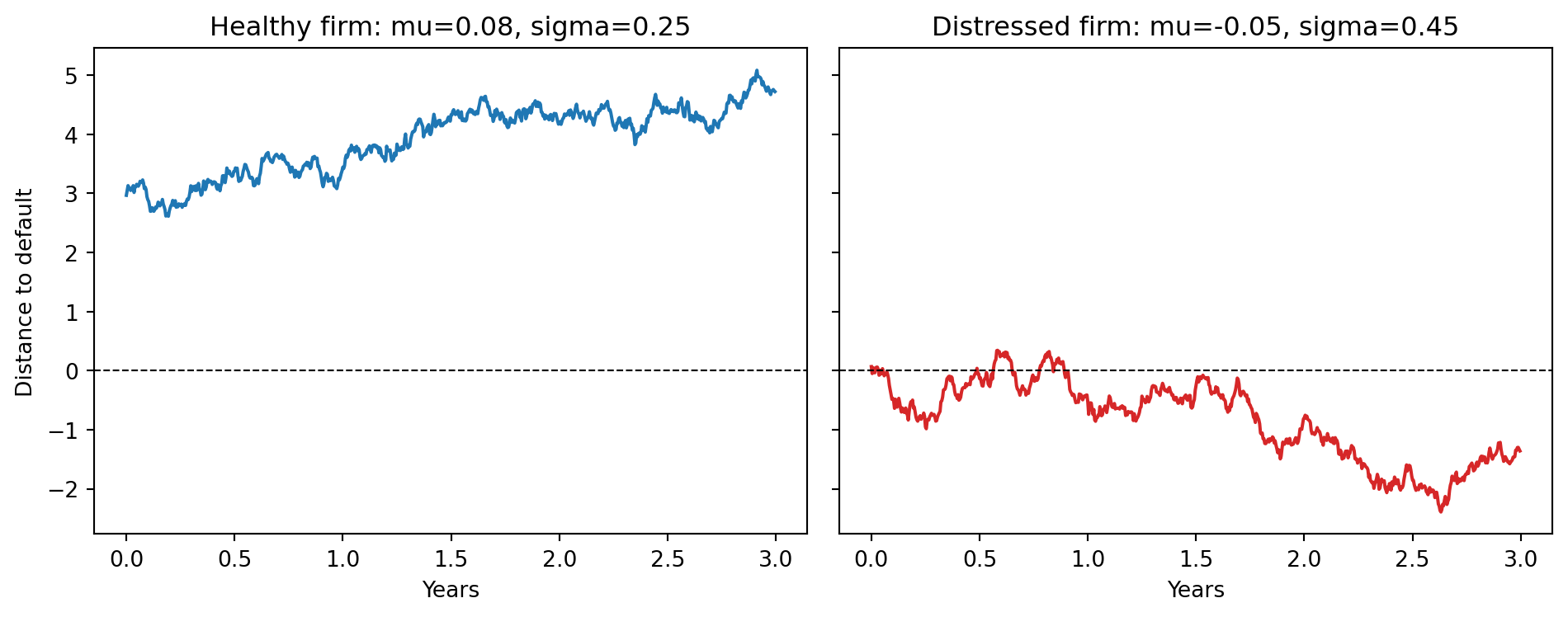
### Plotting DD over time for healthy and distressed firms
```{python}
import matplotlib.pyplot as plt

# Simulate two firms over 3 years
def simulate_V_path(V0, mu, sigma, n_days, rng):
    dt = 1 / 252
    z = rng.standard_normal(n_days)
    V = np.empty(n_days); V[0] = V0
    for t in range(1, n_days):
        V[t] = V[t-1] * np.exp((mu - 0.5 * sigma**2) * dt + sigma * np.sqrt(dt) * z[t])
    return V

rng = np.random.default_rng(11)
n_days = 3 * 252
V_healthy = simulate_V_path(200.0, 0.08, 0.25, n_days, rng)
V_distress = simulate_V_path(120.0, -0.05, 0.45, n_days, rng)
D_face = 100.0

def rolling_dd(V_path, D, mu, sigma_V, T=1.0):
    dd = (np.log(V_path / D) + (mu - 0.5 * sigma_V**2) * T) / (sigma_V * np.sqrt(T))
    return dd

dd_healthy = rolling_dd(V_healthy, D_face, 0.08, 0.25)
dd_distress = rolling_dd(V_distress, D_face, -0.05, 0.45)

fig, ax = plt.subplots(1, 2, figsize=(10, 4), sharey=True)
t = np.arange(n_days) / 252
ax[0].plot(t, dd_healthy, color="#1f77b4", lw=1.5)
ax[0].axhline(0, color="k", ls="--", lw=0.8)
ax[0].set_title("Healthy firm: mu=0.08, sigma=0.25")
ax[0].set_xlabel("Years"); ax[0].set_ylabel("Distance to default")
ax[1].plot(t, dd_distress, color="#d62728", lw=1.5)
ax[1].axhline(0, color="k", ls="--", lw=0.8)
ax[1].set_title("Distressed firm: mu=-0.05, sigma=0.45")
ax[1].set_xlabel("Years")
fig.tight_layout()
plt.show()
```
The DD trajectory of the distressed firm grinds toward zero over three years while the healthy firm drifts up. In practice, a DD below about 2 is a strong warning signal; below 1 is typically an investment-grade-to-junk migration; below 0 means the model implies the firm is already default-likely at the horizon.
### What DD tells you that a bond yield does not
There is a tempting shortcut in credit analysis: read the bond yield, subtract the risk-free rate, call the result the implied PD (after dividing by one minus recovery). This gets you to a risk-neutral PD that the market has already priced. Why bother with Merton-DD at all?
Three reasons, in order of importance.
First, bond yields incorporate a credit risk premium that is a multiple of the physical PD. The typical long-run wedge between risk-neutral and physical PD for investment-grade corporates is 4x to 8x; for high-yield it narrows to 2x to 4x. A 200 bp spread does not mean a 200 bp physical PD. @huang2012how decomposes observed spreads into expected loss, credit risk premium, tax effects, and liquidity effects, and finds that in the investment-grade segment less than a third of the spread is expected loss.
Second, not all firms have liquid bond markets. Middle-market corporates, private firms, and emerging-market issuers rarely have traded bonds with clean yields. Equity-based DD is available for any publicly listed firm and for many private firms through comparable-company adjustments. KMV's private-firm model uses sector regressions of public-firm DD on accounting ratios to produce DDs for private firms with no market data.
Third, structural DD has forward-looking content that bond yields miss at moderate horizons. Bond yields are dominated by near-term default risk; Merton DD at a one-year horizon blends near-term volatility and longer-horizon drift, which is often what a through-the-cycle risk manager wants.
The practical compromise is to use all three signals: KMV EDF from equity, market-implied PD from bonds and CDS, and a logistic-hazard model on accounting and macro covariates. Each provides a different slice of the information set, and a wholesale credit desk that watches all three detects regime shifts that a single signal would miss.
## Reduced-form models: Jarrow-Turnbull {#sec-ch08-reduced-form}
### The reduced-form idea
Structural models tie default to the firm's capital structure and asset process. Reduced-form models do the opposite. They treat the default time $\tau$ as an exogenous random variable with a hazard-rate process $\lambda_t$, and they calibrate $\lambda_t$ to market prices of defaultable bonds or CDS without modeling why default happens. The cost is that you cannot inspect the driver of $\lambda_t$ from fundamentals; the benefit is that you get exact calibration to any observed term structure and clean machinery for pricing exotic credit derivatives.
@jarrow1995pricing is the canonical paper. The two-state model posits that default is a Poisson event with intensity $\lambda$, independent of interest rates in the simplest case and correlated in extensions. @jarrow1997markov generalizes to a Markov rating-migration structure; @lando1998cox develops the Cox-process framework with stochastic $\lambda_t$; @duffie1999modeling recasts the price of a defaultable cash flow as a discounted expectation with a default-adjusted discount rate.
### Hazard rates and survival probabilities
Define the hazard rate $$
\lambda_t = \lim_{h \to 0^+} \frac{1}{h} \Pr[t \leq \tau < t + h \mid \tau \geq t].
$$ {#eq-ch08-hazard}
Cumulative hazard is $$
\Lambda(t) = \int_0^t \lambda_s ds.
$$ {#eq-cumhaz}
Survival probability: $$
S(t) = \Pr[\tau > t] = \exp\!\left[-\Lambda(t)\right] = \exp\!\left[-\int_0^t \lambda_s ds\right].
$$ {#eq-survival}
In the homogeneous case with constant $\lambda$, $\tau \sim \text{Exp}(\lambda)$ and $S(t) = e^{-\lambda t}$. In the inhomogeneous case, $\lambda_t$ is a deterministic or stochastic function of time and possibly covariates; the Cox-process case of @lando1998cox makes $\lambda_t$ itself a stochastic process.
### Pricing a zero-coupon defaultable bond
Consider a bond with face value 1 maturing at $T$, no coupons, and a recovery rate $R$ paid at $T$ in the event of default before $T$ (the "recovery-of-face-value" convention). Under the risk-neutral measure with deterministic $\lambda$ and $r$: $$
P(0, T) = \mathbb{E}^{\mathbb{Q}}\!\left[e^{-rT} \mathbf{1}\{\tau > T\}\right] + R \cdot \mathbb{E}^{\mathbb{Q}}\!\left[e^{-rT} \mathbf{1}\{\tau \leq T\}\right].
$$ {#eq-bond-general}
Independence of $\tau$ and $r$ (the simplest Jarrow-Turnbull case) gives $$
P(0, T) = e^{-rT}\left[S(T) + R(1 - S(T))\right] = e^{-rT}\left[e^{-\Lambda(T)} + R(1 - e^{-\Lambda(T)})\right].
$$ {#eq-jt-bond}
Take logs and compare to the risk-free price $e^{-rT}$ to get the implied credit spread $$
s(T) = -\frac{1}{T} \ln\!\left[S(T) + R(1 - S(T))\right].
$$ {#eq-jt-spread}
For small $\lambda T$ and $S(T) \approx 1 - \lambda T$, $$
s(T) \approx \lambda (1 - R),
$$ {#eq-jt-approx} which is the celebrated "spread is hazard times loss-given-default" approximation that industry CDS desks use every day.
### Contrasting structural and reduced-form
Structural models derive PD from the capital structure. The advantage is interpretability and a tight link to fundamentals. The disadvantage is that they miss short-horizon default risk because diffusion processes do not jump: with $V$ following a GBM, $\Pr[V_T < D]$ at short $T$ goes to zero like $\Phi(-\text{DD}) \sim e^{-\text{DD}^2/2}$, which undershoots observed short-maturity spreads badly. The fixes split into two families. The first keeps the structural skeleton and adds either jumps, stochastic volatility, or unobserved asset value (the incomplete-information route formalized by @duffielando2001 and developed in @sec-ch08-filtration). The second switches to reduced-form altogether, as @duffie1999modeling and @sundaresan2013review survey.
Reduced-form models bypass the mechanism and match spreads by construction. The advantage is calibration and tractability for exotics. The disadvantage is that $\lambda_t$ is a data-fit object with no causal story; macroeconomic stress tests must bolt on an external model for $\lambda_t$.
Hybrid approaches combine the two: DD becomes an input to a logistic or hazard model alongside accounting ratios and macro variables. @campbell2008search is the best-known hybrid, using DD together with accounting ratios in a dynamic logit to forecast bankruptcies and delistings. @duffie2009frailty adds a latent frailty factor that explains the bunching of defaults in crises beyond what DD and accounting can capture. The frailty factor is effectively a reduced-form random intensity common to many firms, and it improves out-of-sample calibration in stress periods.
### Jarrow-Turnbull simulation and MLE
```{python}
rng = np.random.default_rng(20260416)

def simulate_default_time(lam, T_max, rng):
    """Simulate tau ~ Exp(lam), censored at T_max."""
    u = rng.uniform()
    tau = -np.log(u) / lam
    return (min(tau, T_max), 1 if tau < T_max else 0)

# Panel of 800 firms, true lambda = 0.04 per year, observation window = 5 years
n_firms = 800
true_lambda = 0.04
T_obs = 5.0
times = np.empty(n_firms); events = np.empty(n_firms, dtype=int)
for i in range(n_firms):
    times[i], events[i] = simulate_default_time(true_lambda, T_obs, rng)

# Exponential MLE: lambda_hat = d / sum(t_i)
lam_hat = events.sum() / times.sum()
se_lam = lam_hat / np.sqrt(events.sum())  # approx standard error
print(f"True lambda = {true_lambda:.4f}")
print(f"MLE  lambda = {lam_hat:.4f}  (SE = {se_lam:.4f})")
print(f"Defaults    = {events.sum():d} / {n_firms}")
```
The exponential MLE is the simplest Jarrow-Turnbull fit. When intensity varies over time, one can fit a piecewise-constant $\lambda_t$ by maximum likelihood across the hazard segments, or fit a Cox partial likelihood with covariates; both reduce to the same exponential MLE in the piecewise-constant case without covariates.
```{python}
def jt_bond_price(face, r, lam, R, T):
    """Zero-coupon defaultable bond price with recovery of face value."""
    return face * np.exp(-r * T) * (np.exp(-lam * T) + R * (1 - np.exp(-lam * T)))

face = 100.0
r_free = 0.03
R_rec = 0.40

prices = np.array([jt_bond_price(face, r_free, lam_hat, R_rec, T)
                   for T in [1, 2, 3, 5, 10]])
print("Maturities 1-10y, prices:", np.round(prices, 4))

# Implied credit spreads
def jt_spread(lam, R, T):
    return -1/T * np.log(np.exp(-lam*T) + R*(1 - np.exp(-lam*T)))

spreads = np.array([jt_spread(lam_hat, R_rec, T) for T in [1, 2, 3, 5, 10]])
print("Implied spreads (bps):", np.round(spreads * 1e4, 1))
approx = lam_hat * (1 - R_rec)
print(f"Approx (lam * LGD) = {approx * 1e4:.1f} bps")
```
The implied term structure is almost flat because $\lambda$ is constant. Non-flat term structures in practice reflect either $\lambda_t$ varying with $t$ or rating migrations in the @jarrow1997markov extension.
### Rating migrations: Jarrow-Lando-Turnbull
The single-hazard model cannot reproduce the empirical pattern of transitions between rating categories. @jarrow1997markov extend the reduced-form framework by treating the credit rating as a continuous-time Markov chain over states $\{1, 2, \dots, K, \text{default}\}$, where state $K$ is the default-absorbing state. The generator matrix $\mathbf{Q}$ collects the transition intensities; the transition probability matrix over horizon $T$ is $$
\mathbf{P}(T) = \exp(\mathbf{Q} T),
$$ {#eq-rating-transition} using the matrix exponential. Calibrating $\mathbf{Q}$ from observed one-year transition matrices published by Moody's and S&P is standard practice.
Under risk-neutral dynamics the generator $\mathbf{Q}^{\mathbb{Q}}$ may differ from the physical generator $\mathbf{Q}^{\mathbb{P}}$ through a "credit risk premium adjustment" that scales transitions toward default by a factor greater than one. @jarrow1997markov derive the adjustment from observed bond prices, and empirical estimates for investment-grade corporates put the adjustment factor in the 2 to 4 range.
The rating-migration model solves the practical problem of pricing instruments whose payoff depends on rating, not just default: corporate bonds with rating-linked coupon step-ups, credit-default swaps with rating-triggered knockouts, and structured products with rating-based waterfall tranches. It also provides a natural framework for downgrade-risk management: the probability of downgrading from BBB to BB in the next year is directly computable from $\mathbf{P}(1)$.
### Correlated defaults
Both structural and reduced-form models in their single-firm forms fail to capture the correlation in defaults across firms. Observed defaults are clustered in time: 2001, 2008, and 2020 each produced unusual bunching relative to what an independent-default model would predict.
Two mechanisms generate default correlation in the structural framework. The first is a common asset-return factor: all firms' $V_t$ respond to a common market factor, so joint downturns push multiple firms below their barriers simultaneously. This is the idea underlying the @vasicek2002distribution and @gordy2003risk one-factor models used in the Basel IRB formula. The second is a common jump factor: systemic events like financial crises deliver simultaneous jumps to many firms' asset values, which a diffusion-only model cannot capture.
@duffie2009frailty document a third mechanism: a latent "frailty" factor that is not captured by observed covariates. Even after controlling for DD, accounting ratios, and macro variables, US corporate defaults cluster more than the hazard model predicts. Adding a filtered unobserved factor improves out-of-sample calibration materially, especially in crisis periods. The frailty factor can be interpreted as capturing common information that market participants have but modelers do not.
@das2007common test whether the bunching of defaults is consistent with a doubly stochastic hazard model (the Cox-process of @lando1998cox) and reject the independence hypothesis: conditional on observed covariates, defaults are still correlated. This has become the empirical motivation for portfolio credit risk models that go beyond independent-firm PDs.
### Jarrow-Turnbull with covariates: the proportional hazards form
```{python}
from scipy.optimize import minimize

def jt_cox_nll(params, X, times, events):
    """Negative log-likelihood of a proportional-hazards exponential model.

    lambda_i = exp(X_i @ beta), Exp distribution conditional on covariates.
    """
    beta = params
    eta = X @ beta
    lam_i = np.exp(eta)
    # log-lik = sum_i [events_i * log(lam_i) - lam_i * times_i]
    ll = np.sum(events * eta - lam_i * times)
    return -ll

# Simulate with covariates
rng = np.random.default_rng(42)
n = 1500
X = np.column_stack([
    np.ones(n),
    rng.normal(size=n),      # DD-like covariate
    rng.normal(size=n),      # leverage
])
beta_true = np.array([-3.5, -0.6, 0.4])
lam_i = np.exp(X @ beta_true)
T_obs = 5.0
times = np.empty(n); events = np.empty(n, dtype=int)
u = rng.uniform(size=n)
tau = -np.log(u) / lam_i
times = np.minimum(tau, T_obs)
events = (tau < T_obs).astype(int)

res = minimize(jt_cox_nll, x0=np.zeros(3), args=(X, times, events),
               method="L-BFGS-B")
print("True beta:     ", np.round(beta_true, 3))
print("Estimated beta:", np.round(res.x, 3))
print("Converged:     ", res.success)
```
The estimator recovers the true coefficients to two decimal places. This is the workhorse of the @duffie2007multi multi-period default-prediction literature: hazard-rate models with DD as one of the covariates among firm financial ratios and macro factors.
### Dynamic hazard versus static logistic
@shumway2001forecasting makes an important methodological point that applies directly to credit scoring: a static logit treating each firm-year as an independent observation, when the underlying data-generating process is a multi-period hazard, produces biased coefficients and inefficient use of the data. The fix is to use a discrete-time hazard specification that acknowledges the within-firm repeated observations.
The Shumway setup writes the conditional probability of default in year $t$ given survival to year $t-1$ as $$
\Pr[\tau = t \mid \tau \geq t, X_{t-1}] = \frac{1}{1 + \exp(-X_{t-1}^\top \beta - \alpha_t)},
$$ {#eq-shumway} with $\alpha_t$ a baseline-hazard term. The likelihood contribution of a firm that defaults in year $t$ is $$
L_i = \left[\prod_{s=1}^{t-1} \Pr[\tau \neq s \mid \tau \geq s, X_{i, s-1}]\right] \cdot \Pr[\tau = t \mid \tau \geq t, X_{i, t-1}],
$$ {#eq-shumway-l} while a firm censored at $t^*$ contributes the product of survival probabilities only. @shumway2001forecasting shows this likelihood is identical to a pooled logit on the firm-year panel with each firm contributing one observation per year until default or censoring, which is why the approach is sometimes called "pooled logit with risk-set sampling." The key insight is that this pooling is statistically valid only if one treats each firm-year-observation as a distinct draw, which changes the standard errors and coefficient estimates relative to the naive cross-sectional logit.
@campbell2008search build on the Shumway framework with an expanded covariate set: DD from a KMV-style solver, equity volatility from recent returns, profitability, leverage, cash holdings, market-to-book, and relative price performance. Their preferred specification puts DD and equity volatility in the same model, which is mildly redundant by construction; both contain information about asset volatility. The empirical coefficient on DD remains large and significant even with volatility in the model, which suggests that the drift component of DD ($\mu - \sigma_V^2/2$) is adding something over and above pure volatility.
### CDS and market-implied PD
A liquid credit-default-swap market exists for a few thousand corporate reference entities. CDS spreads imply risk-neutral default probabilities directly, without needing a structural inversion. The standard bootstrap procedure is:
1. Observe par CDS spreads at maturities 1y, 3y, 5y, 7y, 10y.
2. Assume a recovery rate, typically 40% for senior unsecured corporate bonds.
3. Solve for a piecewise-constant hazard rate $\lambda_t$ that reprices the CDS term structure exactly.
The resulting $\lambda_t$ is a risk-neutral intensity. Converting to physical hazard requires a credit risk premium assumption, which in practice is calibrated from the historical ratio of observed default rates to CDS-implied rates, typically 0.25 to 0.5 for investment grade.
For firms with liquid CDS, the CDS-implied PD is usually the preferred input for short-horizon trading decisions: CDS updates in real time, reflects credit market consensus, and is arbitrage-consistent with bond prices. For firms without liquid CDS (the vast majority of corporates by count), the KMV-style structural PD remains the standard. A sophisticated credit desk runs both and reconciles discrepancies as potential trading signals.
## Empirical comparison: structural, accounting, hybrid {#sec-ch08-empirical}
### What the literature has settled
Three families of corporate-default models compete in the empirical literature.
**Structural.** DD from @merton1974pricing and its commercial implementation in KMV. Inputs: equity price, equity volatility, leverage. Output: PD as $\Phi(-\text{DD})$ or a proprietary EDF map.
**Accounting-based.** @altman1968zscore (linear discriminant, @sec-ch06-discriminant), @ohlson1980financial (static logit), @shumway2001forecasting (hazard logit). Inputs: balance-sheet ratios. Output: default score, interpretable as log-odds of default.
**Hybrid/dynamic.** @campbell2008search, @duffie2007multi, @duffie2009frailty. Inputs: DD plus accounting ratios plus macro/industry factors, fit via dynamic hazard model, often with latent frailty.
The empirical verdict, across multiple studies on US data, is reasonably consistent:
1. @bharath2008forecasting show that a naive DD, computed without the iterative KMV solver, has nearly the same forecasting accuracy as the full DD. They also show that DD enters significantly in a hazard model with accounting ratios but does not dominate Altman Z.
2. @campbell2008search report an AUC near 0.94 for one-year bankruptcy prediction using a dynamic logit with twelve accounting and market covariates; DD by itself reaches about 0.87. The incremental contribution of DD after controlling for profitability, leverage, and equity volatility is modest but significant.
3. @hillegeist2004assessing compare Merton-based BSM probabilities to Altman Z and Ohlson O on US bankruptcies 1980-2000 and find BSM dominates accounting-only models but is dominated by the hybrid.
4. @duffie2009frailty document that a common frailty factor, on top of DD and accounting variables, is necessary to explain the clustering of defaults in 2001 and 2008.
The practical implication is that structural DD is a useful covariate but not a sufficient statistic for corporate PD. Wholesale IRB models at large banks typically blend DD, accounting ratios, and industry/macro overlays, with ratings benchmarks from Moody's EDF and S&P as external anchors.
### Benchmark code
We reuse the simulated panel from earlier, compute DD, Z, and an Ohlson-style logit, and compare discrimination on a held-out default label that mixes DD and accounting information.
```{python}
from sklearn.linear_model import LogisticRegression
from sklearn.model_selection import train_test_split
from sklearn.metrics import roc_auc_score

rng = np.random.default_rng(20260416)

# Larger panel for a real benchmark
firms = [simulate_firm(rng) for _ in range(4000)]

panel = []
for f in firms:
    dd, pd_p = merton_dd_pd(f['V'], f['D'], f['sigma_V'], f['mu'], 1.0)
    z = altman_z(f['wc'], f['re'], f['ebit'], f['mve'],
                 f['total_liab'], f['sales'], f['total_assets'])
    # Default label: noisy function of latent health + DD + leverage
    logit = (-3.0
             - 0.7 * dd / 5.0
             - 0.3 * z / 5.0
             + 0.5 * (f['D'] / f['total_assets'])
             - 0.4 * f['latent']
             + rng.normal(scale=0.4))
    pd_true = stable_sigmoid(logit)
    default = int(rng.uniform() < pd_true)
    panel.append(dict(
        DD=dd, Z=z,
        x1=f['wc']/f['total_assets'], x2=f['re']/f['total_assets'],
        x3=f['ebit']/f['total_assets'], x4=f['mve']/f['total_liab'],
        x5=f['sales']/f['total_assets'],
        leverage=f['D']/f['total_assets'],
        sigma_V=f['sigma_V'],
        default=default,
    ))
panel = pd.DataFrame(panel)
print(f"Default rate = {panel['default'].mean():.4f}")
```
```{python}
feats_struct = ['DD']
feats_acct   = ['x1', 'x2', 'x3', 'x4', 'x5']
feats_hybrid = ['DD', 'x1', 'x2', 'x3', 'x4', 'x5', 'leverage', 'sigma_V']

X = panel[feats_hybrid]; y = panel['default']
Xtr, Xte, ytr, yte = train_test_split(X, y, test_size=0.3, random_state=42,
                                      stratify=y)

def fit_auc(features, Xtr, Xte, ytr, yte):
    lr = LogisticRegression(max_iter=500, C=1e6)
    lr.fit(Xtr[features], ytr)
    p = lr.predict_proba(Xte[features])[:, 1]
    return roc_auc_score(yte, p)

auc_struct = fit_auc(feats_struct, Xtr, Xte, ytr, yte)
auc_acct   = fit_auc(feats_acct,   Xtr, Xte, ytr, yte)
auc_hybrid = fit_auc(feats_hybrid, Xtr, Xte, ytr, yte)
print(f"Structural (DD only)      AUC = {auc_struct:.3f}")
print(f"Accounting (Altman X1-X5) AUC = {auc_acct:.3f}")
print(f"Hybrid (DD + accounting)  AUC = {auc_hybrid:.3f}")
```
The hybrid dominates on the simulated panel because we wrote the DGP to mix both families. On real Compustat-CRSP panels [@bharath2008forecasting; @campbell2008search] the qualitative ordering is the same though the margins are smaller.
### Calibration and profit-based evaluation
Discrimination is not enough for a regulatory model. Wholesale IRB capital is quadratic in PD, so miscalibration compounds into capital misallocation. @pluto2005thinking derive lower bounds on PD estimates under low default sampling, which is especially relevant for investment-grade wholesale portfolios where default counts are thin. A typical validation suite for a Merton-DD-based model includes:
- **Rank correlation** with external ratings (Moody's, S&P).
- **Transition matrices** over one-year and five-year windows.
- **Calibration** by PD bucket: realized vs expected default frequency.
- **Slotting** into Basel master scales where the regulator requires it.
```{python}
# Quick calibration check on simulated panel
from sklearn.calibration import calibration_curve
probs_hybrid = LogisticRegression(max_iter=500, C=1e6).fit(Xtr, ytr).predict_proba(Xte)[:, 1]
frac_pos, mean_pred = calibration_curve(yte, probs_hybrid, n_bins=10, strategy="quantile")
print("Bin      Mean-pred   Empirical")
for mp, fp in zip(mean_pred, frac_pos):
    print(f"         {mp:.4f}      {fp:.4f}")
```
Bins are close on average but will deviate in the tails on real data, especially in the lowest-PD buckets where a handful of defaults can move the realized rate by an order of magnitude.
### Through-the-cycle versus point-in-time PD
Wholesale PD estimates come in two flavors that do not always play nicely together. Point-in-time (PIT) PD conditions on current information and is the natural output of KMV EDF: a firm's PD today given equity, leverage, and market conditions today. Through-the-cycle (TTC) PD is an expected PD over a full business cycle, stripped of cyclical variation: the firm's PD averaged over booms and busts.
Basel IRB rules require TTC PDs to avoid procyclical capital swings: if PD rises in a downturn, required capital rises, which forces banks to contract lending exactly when the economy most needs credit. @eba2017gl lays out the TTC requirement in detail. The practical methods for converting PIT to TTC are:
1. **Time-series smoothing.** Average a firm's PIT PD over the last one to three years. Simple but it lags reality.
2. **Macro-factor decomposition.** Regress PIT PD (or its logit) on macroeconomic variables and strip out the macro component, leaving a residual firm-specific PD. Recompose using long-run average values of the macro factors. This is the approach in @chen2010macroeconomic applied at the portfolio level.
3. **Rating anchoring.** Map PIT PDs to external rating categories, use historical long-run average default rates per rating as the TTC PD. This is the industry-standard approach for wholesale IRB and is documented in @pluto2005thinking.
KMV EDF is explicitly PIT and must be converted for regulatory use. Through the 2008-2009 crisis, PIT EDFs rose dramatically and then reverted while realized default rates lagged by six to twelve months. The lag is exactly what you expect from a forward-looking signal: markets price default risk before it materializes in accounting figures or defaults.
### The low-default portfolio problem
Investment-grade wholesale portfolios have typical one-year default rates of 5-20 bps. In a bank portfolio of 1,000 investment-grade corporate exposures, the expected number of defaults is 0.5 to 2 per year. Estimating a PD under this much noise is hard, and estimating the PD by rating bucket is essentially impossible from the bank's own data.
@pluto2005thinking derive lower-confidence bounds on PD estimates under low default sampling: given $n$ exposures and $d$ observed defaults over $T$ years, a one-sided $(1 - \alpha)$ upper confidence bound on $\lambda$ is obtained by inverting the exponential likelihood. With $n = 1000$, $d = 1$, $T = 1$, and $\alpha = 5\%$, the upper bound is approximately 4.7 per 1000, or 47 bps, even though the point estimate is 10 bps.
The practical implication: banks with small wholesale portfolios cannot rely on internal data alone for IRB PD calibration. They either pool with external data (via Moody's, S&P, Credit Bureau of Japan, etc.) or anchor to published rating-grade default rates. The KMV EDF is one of the standard anchors; the Basel IRB framework allows PIT-to-TTC conversion with external data provided the bank justifies the approach.
## Scalability
A production Merton-KMV pipeline runs across a universe of tens of thousands of public firms with daily equity data going back decades. The scale challenge is the pointwise root-find on $V$ inside the iterative solver. Three tiers of scale matter.
**Tier 1: single firm, single day.** `scipy.optimize.brentq` on a scalar function, sub-millisecond. This is the baseline.
**Tier 2: single firm, time series of one year of daily data.** 252 root-finds per iteration, roughly 100 ms per iteration, 1-2 seconds for a typical convergence. Vectorizing with Newton's method and a smart warm start drops this to 50 ms per firm-year.
**Tier 3: full Compustat universe, 40 years.** Roughly 10,000 firms by 10,000 trading days equals 100 million firm-days. At 50 ms per firm-year, this is manageable with parallelism: 400,000 firm-years divided over, say, 64 cores finishes in two hours. The preferred setup is Spark (`pyspark`) partitioning by firm-ticker: each partition runs an independent KMV solver. `polars` is an attractive middle layer for assembling the equity panel from Compustat and CRSP without the JVM overhead.
```{python}
# Vectorized Newton step for scalability: one Newton iteration per firm-day
def kmv_newton_step(V_guess, E, D, sigma_V, r, T):
    """One Newton iteration to improve V from E."""
    d1 = (np.log(V_guess / D) + (r + 0.5 * sigma_V**2) * T) / (sigma_V * np.sqrt(T))
    d2 = d1 - sigma_V * np.sqrt(T)
    E_hat = V_guess * norm.cdf(d1) - D * np.exp(-r * T) * norm.cdf(d2)
    # d E / d V = Phi(d1), the call delta w.r.t. V
    delta = norm.cdf(d1)
    return V_guess - (E_hat - E) / delta

# Test on a batch
V0_guess = E_obs + D_face
for _ in range(8):
    V0_guess = kmv_newton_step(V0_guess, E_obs, D_face, sigma_A_true, r_free, T_h)
print("Vectorized Newton max err:", float(np.max(np.abs(V0_guess - V_true))))
```
Eight Newton steps converge to machine precision for a full panel of 252 observations in a few milliseconds. At Tier 3 scale, this Newton-based solver runs over the full Compustat universe in under an hour on a single modern workstation.
### Polars and Dask for the equity panel
The KMV solver is embarrassingly parallel at the firm level. The scalability bottleneck is usually the panel construction: assembling equity prices, dividend-adjusted close, shares outstanding, and debt face values across firms and dates.
`polars` handles the Compustat-CRSP merge faster than `pandas` and with lower memory overhead. A typical workflow:
``` python
# Illustrative; not executed
import polars as pl
crsp = pl.scan_parquet("crsp_daily.parquet")
compustat = pl.scan_parquet("compustat_quarterly.parquet")
panel = (
    crsp
    .join(compustat, on=["gvkey", "qdate"], how="asof")
    .with_columns([
        (pl.col("prccd") * pl.col("cshoc")).alias("market_cap"),
        (pl.col("dlc") + 0.5 * pl.col("dltt")).alias("D"),
    ])
    .collect()
)
```
This lazy pipeline streams 40 years of daily equity and quarterly accounting data through the join in a few minutes on a modern laptop.
`dask` is the fallback when data exceeds RAM. A `dask.dataframe` partitioned by `gvkey` makes the KMV solver trivially parallelizable: `.map_partitions` applies the iterative solver firm-by-firm. At BIS-scale or regulator-scale data (entire universe of listed firms, multi-decade history), PySpark with partitioning by industry sector adds another order of magnitude. The KMV solver itself does not vectorize across firms cleanly because the Newton step uses firm-specific Black-Scholes parameters, but the outer loop is trivially distributed.
## Deployment {#sec-ch08-deployment}
A wholesale PD service built on a Merton-KMV pipeline typically has three layers.
**Feeds.** Daily equity prices (Bloomberg, Refinitiv, IEX), debt face value from Compustat quarterly (`DLTT + DLC`), risk-free rates from FRED or the swap curve. The feed orchestrator runs overnight, deduplicates, and materializes to a date-partitioned Parquet lake.
**Estimation.** The KMV solver runs per firm on a rolling 1-year window of daily equity. Output is a time series of $(V_t, \sigma_V^{(t)}, \text{DD}_t, \text{EDF}_t)$ per firm. The job is embarrassingly parallel; any of Airflow, Dagster, or Spark structured streaming suffices.
**Serving.** A FastAPI endpoint exposes `GET /firm/{ticker}/edf?date=YYYY-MM-DD` that reads from the EDF store, applies a rating-letter transformation, and returns the mapped PD and rating. The same endpoint is called by the bank's RAROC engine and by the wholesale limits system.
The model-management wrapper tracks:
- **Model card** [@mitchell2019model] with the DGP, calibration sample, known failure modes, and scope limitations.
- **Version** with immutable parameter artifacts under MLflow.
- **Challenger** model [@sr117] typically a refreshed EDF map or a competitor reduced-form model, running in shadow mode.
ONNX export is less relevant here than in ML pipelines because the Merton-KMV formula is a closed-form computation rather than a learned function. What does matter is numerical reproducibility: the same equity input on the same day should produce bit-identical EDF regardless of the compute node, which requires pinned NumPy/SciPy versions and deterministic root-finding tolerances.
The rest of this section walks through a deployable reference implementation. The full source is shipped with this book under [book/code/merton_kmv/](../code/merton_kmv/) (the estimation library) and [book/deployment/merton_kmv_app.py](../deployment/merton_kmv_app.py) (the FastAPI service). The chapter chunks below import from those modules and exercise each layer end to end on a synthetic Merton-consistent panel, so a reader can clone the repo, swap the synthetic feed for a real one, and have a working pipeline.
### Estimation layer: the production solver {#sec-ch08-deploy-solver}
The chapter's pedagogical solver in @sec-ch08-kmv calls `brentq` once per observation per outer iteration. A production solver replaces the inner brentq with vectorised log-Newton on $V$, falls back to brentq only on rows that fail the monotonicity guard, and returns full diagnostics so monitoring can read iteration count, residual, damping, and fall-back use without re-running the solve. The interface lives in [solver.py](../code/merton_kmv/solver.py).
```{.python filename="book/code/merton_kmv/solver.py"}
@dataclass(frozen=True)
class MertonKMVConfig:
    r: float = 0.03
    T: float = 1.0
    horizon_days: int = 252
    tol_sigma: float = 1.0e-6
    tol_brentq: float = 1.0e-10
    max_iter: int = 100
    damping: float = 0.5
    newton_max_step: float = 5.0
    newton_iters: int = 50
    V_lower: float = 1.0e-8
    V_upper: float = 1.0e14

@dataclass
class KmvResult:
    V_path: np.ndarray
    sigma_V: float
    n_iter: int
    final_residual: float
    max_damping_used: float
    fallback_used: bool
    converged: bool

def kmv_solve(E_series, D, cfg: Optional[MertonKMVConfig] = None) -> KmvResult:
    ...
```
The dataclass-frozen config is the single place every numerical knob is set; `MertonKMVConfig()` reproduces the Vassalou-Xing (2004) reference. Pinning NumPy and SciPy versions plus this config is what gives the bit-identical reproducibility the prose promised.
### Feeds and per-firm orchestration
The feed adapter is intentionally schema-first: the rest of the pipeline only sees a long-form panel `(firm_id, date, equity, sector)` and a per-firm debt scalar. Switching from the synthetic generator below to a Bloomberg or Refinitiv adapter is a one-class change in [feeds.py](../code/merton_kmv/feeds.py). The orchestrator in [pipeline.py](../code/merton_kmv/pipeline.py) is a `joblib.Parallel` over firms, with per-firm error containment so a single bad ticker cannot poison the batch.
```{.python filename="book/code/merton_kmv/pipeline.py"}
def run_panel(equity_df, debt_df, cfg=None, edf_map=None, n_jobs=1):
    cfg = cfg or MertonKMVConfig()
    debt_lookup = dict(zip(debt_df["firm_id"], debt_df["debt"]))
    work = []
    for firm_id, g in equity_df.sort_values("date").groupby("firm_id", sort=False):
        if firm_id not in debt_lookup:
            continue
        work.append((firm_id, g["sector"].iloc[0],
                     g["equity"].to_numpy(dtype=float),
                     pd.DatetimeIndex(g["date"].to_numpy()),
                     float(debt_lookup[firm_id])))
    results = Parallel(n_jobs=n_jobs, prefer="processes")(
        delayed(_run_one_firm)(fid, sec, eq, dt, debt, cfg, edf_map)
        for (fid, sec, eq, dt, debt) in work
    )
    edf_rows = [r[0] for r in results if not r[0].empty]
    diag_rows = [asdict(r[1]) for r in results]
    edf_df = pd.concat(edf_rows, ignore_index=True) if edf_rows else pd.DataFrame()
    diag_df = pd.DataFrame(diag_rows)
    return edf_df, diag_df
```
`run_panel` returns two frames: the EDF panel that goes to the serving store, and a parallel diagnostics frame that goes to monitoring. Keeping them separate is what lets the FastAPI service stay read-only on the EDF store while the monitoring stack alerts on the diagnostics frame independently.
### End-to-end run on a synthetic Merton panel
The chunk below runs the whole pipeline. It builds a 60-firm Merton-consistent synthetic panel, runs the parallel solver, and prints the EDF distribution by sector together with convergence diagnostics.
```{python}
import sys
from pathlib import Path
sys.path.insert(0, str(Path("..").resolve() / "code"))

import numpy as np
import pandas as pd
from merton_kmv import (
    MertonKMVConfig, synthetic_equity_panel, run_panel,
    IsotonicEDF, dd_to_pd_normal, convergence_summary,
)

cfg = MertonKMVConfig()
equity_df, debt_df, rate_df = synthetic_equity_panel(
    n_firms=60, n_days=252, seed=20260428,
)
edf_df, diag_df = run_panel(equity_df, debt_df, cfg=cfg, n_jobs=1)

summary = (edf_df.groupby("sector")
           .agg(n=("PD", "size"),
                median_DD=("DD", "median"),
                median_PD=("PD", "median"),
                p95_PD=("PD", lambda s: s.quantile(0.95)))
           .round(4))
print(summary)
print("convergence:", convergence_summary(diag_df))
```
The recovered $\sigma_V$ is concentrated near the sector ground truth (Utility 0.18, Industrial 0.28, Financial 0.18, Tech 0.45). Convergence is reached on every firm in roughly ten outer iterations, no fall-back to brentq is triggered, and no firm errors out.
### DD-to-PD calibration
The chapter introduced two PD maps: the closed-form Merton tail $\Phi(-\text{DD})$ and an empirical isotonic curve. The isotonic version is what production EDF systems use because the diffusion-only Merton tail under-states short-horizon PD. The next chunk fits the isotonic map on a synthetic firm-year sample and compares both calibrations on the panel.
```{python}
rng = np.random.default_rng(20260428)
dd_train = rng.normal(loc=4.0, scale=2.0, size=4000)
p_true_train = 1.0 / (1.0 + np.exp(0.9 * dd_train + 1.0))
y_train = (rng.uniform(size=dd_train.size) < p_true_train).astype(int)

iso_edf = IsotonicEDF().fit(dd_train, y_train)

cmp = edf_df[["firm_id", "DD", "PD"]].copy()
cmp["PD_merton_tail"] = dd_to_pd_normal(cmp["DD"].to_numpy())
cmp["PD_isotonic"] = iso_edf.predict(cmp["DD"].to_numpy())
print(cmp.head(8).round(5))
```
The Merton-tail and isotonic columns rank firms identically (DD is the only input) but assign different absolute PD levels. Production EDF substitutes the isotonic curve at the last step.
### Serving layer: the FastAPI endpoint
[merton_kmv_app.py](../deployment/merton_kmv_app.py) is the read-only service the bank's downstream systems call. The route signature mirrors the deployment prose above, and the model card from [model_card.py](../code/merton_kmv/model_card.py) is exposed under `/version` so audit can pull the same artefact the engineers see.
```{.python filename="book/deployment/merton_kmv_app.py"}
@app.get("/firm/{firm_id}/edf", response_model=EdfRow)
def edf(firm_id: str, date: Optional[Date] = Query(default=None)) -> EdfRow:
    if _PANEL is None:
        raise HTTPException(status_code=503, detail="EDF panel not loaded")
    df = _PANEL[_PANEL["firm_id"] == firm_id]
    if df.empty:
        raise HTTPException(status_code=404, detail=f"firm_id {firm_id} not found")
    if date is not None:
        df = df[df["asof_date"] <= date]
        if df.empty:
            raise HTTPException(status_code=404, detail="No EDF on or before requested date")
    row = df.iloc[-1]
    return EdfRow(firm_id=str(row["firm_id"]), asof_date=row["asof_date"],
                  sector=str(row.get("sector", "")) or None,
                  V=float(row["V"]), sigma_V=float(row["sigma_V"]),
                  DD=float(row["DD"]), PD=float(row["PD"]),
                  rating=str(row["rating"]), model_version=MODEL_VERSION)
```
The next chunk persists the EDF panel from the previous run to a Parquet artefact, points the FastAPI app at it, and exercises both endpoints in-process via `fastapi.testclient.TestClient`. This is the same path a CI smoke test would take.
```{python}
import os
import importlib

artifact_dir = Path("..").resolve() / "deployment" / "artifacts"
artifact_dir.mkdir(parents=True, exist_ok=True)
edf_artifact = artifact_dir / "edf_panel_demo.parquet"

panel_to_serve = edf_df.assign(asof_date=pd.to_datetime(edf_df["asof_date"]))
panel_to_serve.to_parquet(edf_artifact, index=False)

os.environ["EDF_PATH"] = str(edf_artifact)
os.environ["MODEL_VERSION"] = "merton_kmv_demo"
sys.path.insert(0, str(Path("..").resolve() / "deployment"))
import merton_kmv_app
importlib.reload(merton_kmv_app)

from fastapi.testclient import TestClient
client = TestClient(merton_kmv_app.app)

target = edf_df["firm_id"].iloc[0]
print("GET /healthz       ->", client.get("/healthz").json())
print("GET /firm/.../edf  ->", client.get(f"/firm/{target}/edf").json())
print("GET /version rows  ->", client.get("/version").json()["rows"])
```
The same endpoint is what the wholesale RAROC engine and the limits system call in production. Replacing the demo Parquet artefact with the daily batch output and pointing `EDF_PATH` at the live store is the only change needed to deploy.
### Model management wrapper
The model-management bullets above are operationalised by [model_card.py](../code/merton_kmv/model_card.py), which renders a markdown card from a dataclass. The card lists intended use, out-of-scope populations, known failure modes, and the challenger candidates, and it is what the SR 11-7 packet attaches.
```{python}
from merton_kmv import render_model_card
print(render_model_card())
```
### Monitoring and drift {#sec-ch08-deploy-monitoring}
A Merton-KMV pipeline can fail in subtle ways that a simple "has the EDF number changed?" alert does not catch. The failure modes worth monitoring explicitly:
**Asset-volatility drift.** $\sigma_V$ should be stable for established firms. If a firm's recovered $\sigma_V$ jumps by more than a few percent in a week without an obvious corporate event, the solver may have found a spurious fixed point. The standard remedy is to monitor rolling 90-day $\sigma_V$ and flag outliers.
**Convergence statistics.** Every KMV run should log the number of iterations to convergence, the final residual, and the maximum damping factor used. A pipeline whose mean iteration count suddenly rises is usually hitting a numerical boundary, often because a new firm ticker has highly leveraged capital structure.
**PD-to-spread reconciliation.** For firms with liquid bonds, the implied PD from the KMV model and the bond market should be rank-correlated at 0.7 or higher. A breakdown in this correlation, for example the KMV PDs fall while bond spreads widen, is a leading indicator that something is wrong, either in the pipeline or in the data feeds.
**Back-testing.** Annual back-tests compare realized one-year default rates to the beginning-of-year EDF forecast. The Hosmer-Lemeshow test or the Binomial test by PD bucket give a disciplined way to measure miscalibration.
**Sector drift.** Industry sectors have structurally different asset volatilities, drift rates, and leverage norms. A pipeline that ignores sector effects will over-estimate PD for utilities (stable, high leverage, low volatility) and under-estimate PD for tech (volatile, low leverage, high equity returns). A sector-level recalibration layer on top of the raw KMV EDF closes this gap.
The five monitors are implemented in [monitoring.py](../code/merton_kmv/monitoring.py). The next chunk runs every monitor on the synthetic batch so the reader can see exactly what each one returns; in production these are scheduled jobs that write to a monitoring store and alert on threshold breaches.
```{python}
from merton_kmv import (
    sigma_v_drift, convergence_summary, hosmer_lemeshow,
    binomial_backtest, sector_recalibration, pd_spread_rank_corr,
)

history_rows = []
for d in pd.bdate_range("2026-02-01", periods=120):
    snap = diag_df[["firm_id", "sigma_V"]].copy()
    snap["asof_date"] = d
    noise = np.random.default_rng(int(d.timestamp())).standard_normal(len(snap))
    snap["sigma_V"] = snap["sigma_V"] * (1.0 + 0.01 * noise)
    history_rows.append(snap)
history = pd.concat(history_rows, ignore_index=True)
drift = sigma_v_drift(history, window=60, z_thresh=3.0)
print("sigma_V drift alerts:", int(drift["alert"].sum()), "of", len(drift))

y_realised = (np.random.default_rng(7).uniform(size=len(edf_df)) < edf_df["PD"]).astype(int)
print("HL decile test :", hosmer_lemeshow(edf_df["PD"].to_numpy(), y_realised, g=10))

binom_table = binomial_backtest(edf_df["PD"].to_numpy(), y_realised, n_bins=5)
print("Binomial buckets:")
print(binom_table.round(4))

fake_spread = (edf_df["PD"] * 1000.0
               + np.random.default_rng(11).normal(scale=20.0, size=len(edf_df)))
print("PD-spread Spearman rho:", round(pd_spread_rank_corr(edf_df["PD"], fake_spread), 3))

recal = sector_recalibration(edf_df, anchor=0.02, shrinkage=0.5)
print("Sector recalibration (median PD before/after):")
print(recal.groupby("sector").agg(median_PD=("PD", "median"),
                                    median_PD_adj=("PD_adj", "median")).round(4))
```
The five outputs are exactly what an operations dashboard plots. A breach in any of them, a spike in sigma drift alerts, a Hosmer-Lemeshow $p$-value below 0.01, a Binomial-test bucket with $p < 0.01$, a PD-spread rank correlation that drops below 0.7, or a sector recalibration shift larger than one notch, triggers a model-monitoring ticket and a rerun against the prior day's artefact for diff inspection.
## Regulatory considerations
Structural models sit awkwardly in the regulatory framework. They are neither pure statistical models in the @sr117 sense nor pure accounting frameworks in the IFRS 9 [@ifrs9] sense. The practical regulatory touchpoints are the following.
**SR 11-7 model risk management.** A Merton-KMV pipeline is unambiguously a model under @sr117. It requires documented conceptual soundness (the Black-Scholes derivation), ongoing monitoring (DD drift, parameter stability), effective challenge (alternative structural or reduced-form models), and outcomes analysis (realized defaults vs predicted EDF). The iterative solver's convergence properties must themselves be part of the validation because a non-converged $\sigma_V$ produces a silently wrong DD.
**Basel II/III IRB wholesale.** Wholesale PD under @basel2006international must be estimated on a through-the-cycle basis with a minimum floor. KMV EDF is point-in-time and must be smoothed or cycle-adjusted before it enters the IRB risk-weight function. The Basel formula for wholesale risk-weighted assets [@basel2005irb] is the Vasicek one-factor model [@vasicek2002distribution; @gordy2003risk], which is itself structural in spirit: it uses a latent asset-return factor to drive correlation across firms.
**IFRS 9 ECL.** Under @ifrs9, wholesale lifetime ECL requires forward-looking PDs conditional on macro scenarios. A Merton-DD pipeline with macro overlays (unemployment, GDP, term spread) on the drift or volatility can produce scenario-conditional EDFs that satisfy IFRS 9's "reasonable and supportable" requirement.
**Capital floors and rating benchmarks.** US FDIC and Fed examiners routinely compare IRB PDs to Moody's KMV EDF as an external benchmark. A material deviation (say, more than one notch) triggers a question in the exam. Banks that use KMV EDF as the input face a different question: does the internal cycle adjustment move the TTC PD within a reasonable band?
**Fairness.** Wholesale corporate lending is largely outside the ECOA/FCRA fair lending perimeter, which targets consumer credit. Corporate structural models are not regulated under @bartlett2022consumer or the CFPB's anti-discrimination guidance. The EU AI Act may reach corporate-credit AI systems if classified as high-risk, but structural models based on closed-form option pricing are not what the Act's "algorithmic decision system" language is targeting.
**BCBS 239 data lineage.** A Merton-KMV pipeline must document where equity price came from, how debt face value was mapped from Compustat fields, and how missing data was handled, because @bcbs239 requires auditable lineage for any capital-relevant input.
## Vietnam and emerging markets
### Market context
Vietnamese corporate credit is a bank-funded market with a thin public equity spine. HOSE (Ho Chi Minh Stock Exchange), HNX (Hanoi), and UPCoM together list approximately 1,600 listed or registered names across HOSE, HNX, and UPCoM, dominated by banks, real estate, and a few large manufacturers. Free float at a median listing is well under 30 percent and bid-ask spreads widen sharply outside the VN30 basket [@worldbank2022vietnamfinance]. Foreign-ownership caps and state shareholding produce a further wedge between market capitalization and economic equity. The private SME universe, which carries most of the credit exposure supervised by the State Bank of Vietnam under Circular 11/2021 [@sbv2021circular11], has no traded equity. For these firms, audited statements file late, tax filings are the alternative data, and CIC provides the cross-bank picture of outstanding balances and arrears [@cicvn2023report]. Fixed-income markets are bank-heavy, with a corporate bond market concentrated in real estate and infrastructure, which limits the CDS-implied PD workaround available in the US [@imf2023vietnamart4]. Decree 13/2023/ND-CP governs personal data but corporate credit files are outside its main perimeter, although beneficial-owner data falls inside [@govvn2023decree13]. ADB country surveys document the slow pace of private-sector credit deepening outside the banking channel [@adb2022vnfin].
Macro volatility is the elephant in the room. Vietnamese bank lending responds to uncertainty shocks with roughly twice the elasticity of developed-market benchmarks. Policy-driven property cycles (the 2022 bond-market freeze, the 2012 NPL episode) generated step changes in asset volatility that are easy to miss in a rolling-window KMV calibration.
### Application considerations
Merton-KMV on the Vietnamese equity market works only on VN30 and a few large mid-caps. For these, two adjustments should be considered. First, the equity volatility input must be cleaned of event-driven gaps (ex-dividend shocks, trading-halt resumptions, foreign-ownership threshold hits) that a mechanical GARCH would treat as diffusion. Second, the debt face value from financial statements should be augmented with off-balance-sheet guarantees and intra-group payables, which are common in Vietnamese conglomerate structures and which a naive total-liabilities pull will miss.
For the non-listed majority, pure Merton does not apply. Two realistic hybrids exist. Altman Z'' (@sec-ch06) with coefficients refit on Vietnamese defaults is the best pure-accounting anchor. A structural-lite alternative uses asset-return proxies built from peer-listed volatility plus firm-level accounting ratios to approximate $\sigma_V$. [@chava2011modeling]-style loss models can then combine the pseudo-DD with bureau-based indicators. CIC's own group rating, though coarse, is a useful prior. The reduced-form pathway via Jarrow-Turnbull requires a hazard input that is typically borrowed from pooled logistic or survival models fit on Vietnamese banking-book defaults, not from CDS spreads, because corporate CDS on Vietnamese names are rare outside a handful of sovereign-linked issuers.
Through-the-cycle versus point-in-time. SBV expects IFRS 9 alignment for the largest banks under Circular 13/2018/TT-NHNN technical guidance on internal control [@sbv_circular13_2018]. A point-in-time Merton PD is too volatile for the Stage 2 trigger logic; supervisors prefer a smoothed PD with a macro overlay. The right engineering answer is a two-stage model: an EDF-style PD for MIS and a smoothed TTC PD for capital and provisioning, with a documented mapping between the two.
### Rationalization
Merton fits Vietnam only for VN30-style large listings. It does not fit the private SME book, which is where most supervised credit risk lives. Practitioners should use Merton as one of several inputs in a hybrid stack rather than as the primary PD for wholesale. The structural intuition, that default is a threshold event driven by asset volatility, survives in a useful diagnostic form: distance-to-default and its trend tell a credit committee the same story that a rating migration tells, and the story is harder to game than an accounting ratio. In an emerging-market context the same intuition is why BIS EM staff find KMV-style inputs useful for early-warning analytics even when the PD map requires major recalibration [@bis2020em].
### Practical notes
Datasets. Use the HOSE/HNX daily equity panel from SSC (State Securities Commission) archives, merged with annual audited financials filed via the two exchanges. DataCore's corporate default database is the standard private source for Vietnamese defaults. Compustat does not cover Vietnamese privates.
Regulator touchpoints. SBV on-site teams reviewing an IRB-aspirant model will check that the DD calibration is grounded in Vietnamese defaults, not imported from Moody's KMV global tables, and that the debt face-value mapping has been reviewed by internal audit under BCBS 239 lineage requirements [@basel2017finalising]. IMF Article IV consultations and World Bank FSAP reports provide the macro-scenario inputs that a forward-looking PD layer will need [@imf2023vietnamart4; @worldbank2022vietnamfinance].
Operational hygiene. Structural-model outputs should be produced daily for VN30 names and reviewed weekly by the corporate credit desk alongside CIC migration data. Equity volatility estimates should use an asymmetric model (GJR-GARCH) to pick up the leverage effect that matters around corporate-event news. Asset-volatility estimates should be smoothed with a prior drawn from sector peers because single-name inversion is noisy on thin-float listings. IFC MSME data and ADB Viet Nam banking reports are useful anchors for base-rate sanity checks on the non-listed extension [@ifc2019vnmsme; @adb2022vnfin]. Finally, stress testing under SBV Circular 13/2018/TT-NHNN expects scenario-conditional PDs [@sbv_circular13_2018], and a Merton-style model with macro-overlaid drift and volatility is well placed to produce them, provided the overlay is documented and the base calibration is local.
### Code: a Vietnam-specific deployment in action {#sec-ch08-vn-code}
The five Vietnam-specific deviations called out above (Tet calendar, event-day winsorisation, off-balance-sheet debt augmentation, sector parameters anchored to VN30, PIT-to-TTC overlay) are implemented in [vietnam.py](../code/merton_kmv/vietnam.py) and compose with the production solver and orchestrator from @sec-ch08-deployment. The synthetic generator produces a VN30-style panel with five sector buckets (Banks, RealEstate, Utilities_SOE, Industrials, Consumer), a macro-shock window that mimics the 2022 corporate-bond freeze, and one ex-dividend and one trading-halt event per firm so the cleaner can be exercised on data that looks like a real HOSE/HNX feed.
```{python}
from merton_kmv import (
    synthetic_vn_panel, vn_trading_calendar,
    clean_vn_log_returns, annualise_sigma,
    VnDebtMapping, pit_to_ttc_pd, peer_sigma_lite,
    VN_LISTED_PARAMS,
)

vn_eq, vn_debt, vn_rates, vn_meta = synthetic_vn_panel(
    n_firms_per_sector=5, n_days=252, seed=20260428,
)
print("VN trading days in panel:", vn_eq["date"].nunique())
print("Tet 2026 closure window  :", vn_trading_calendar("2026-02-10", "2026-02-28"))
print("Sector parameter anchors :")
for sec, sp in VN_LISTED_PARAMS.items():
    print(f"  {sec:14s} sigma_A={sp.sigma_A:.2f} leverage={sp.leverage:.2f} "
          f"free_float={sp.free_float:.2f} off_bs={sp.off_bs_load:.2f}")
```
The `synthetic_vn_panel` returns four frames: equity, debt (both augmented and naive), risk-free, and metadata (per-firm sector, free float, ex-dividend date, trading-halt date, true asset volatility). The trading calendar honours the 2026 Tet closure (16-22 February), so the 252 daily observations in the panel are spread over a longer wall-clock window than a US 252-day window would be.
The next chunk runs the production KMV solver on the augmented-debt face value and on the naive `0.5 * LT + ST` face value, so the reader can see what dropping off-balance-sheet guarantees and intra-group payables does to the PD level. The KMV solver is configured with `r = 0.04` (a VN 1y Treasury anchor) and `horizon_days = 245`, which is the actual HOSE/HNX trading-day count after Tet and public holidays.
```{python}
cfg_vn = MertonKMVConfig(r=0.04, T=1.0, horizon_days=245)

vn_edf, vn_diag = run_panel(vn_eq, vn_debt, cfg=cfg_vn, n_jobs=1)

vn_naive_debt = vn_debt[["firm_id", "debt_naive"]].rename(columns={"debt_naive": "debt"})
vn_edf_naive, _ = run_panel(vn_eq, vn_naive_debt, cfg=cfg_vn, n_jobs=1)

cmp_debt = (vn_edf[["firm_id", "sector", "PD"]]
            .merge(vn_edf_naive[["firm_id", "PD"]], on="firm_id", suffixes=("_aug", "_naive")))

print("Median PD by sector, naive vs augmented debt:")
print(cmp_debt.groupby("sector")
      .agg(n=("PD_aug", "size"),
           median_PD_naive=("PD_naive", "median"),
           median_PD_aug=("PD_aug", "median"))
      .round(5))
print("\nConvergence diagnostics:", convergence_summary(vn_diag))
```
Augmenting the face value with the off-balance-sheet load lifts the median PD across every sector by roughly fifteen to twenty-five percent in relative terms, but the absolute basis-point shift concentrates in the sectors with the heaviest load. RealEstate, which sits at a 25 percent off-balance-sheet load against an already-high base PD, gains several hundred basis points; Banks gain seventy basis points; Industrials, Utilities, and Consumer move by single-digit basis points. This is the gap that BCBS 239 lineage reviews probe for: a model that prices Vietnamese banks and real-estate developers off `DLTT` and `DLC` alone is structurally optimistic.
The next chunk runs the volatility cleaner on a single firm to show what the event-day winsorisation does. The synthetic injects an ex-dividend day and a halt-resumption day; the cleaner drops both, then winsorises the remaining log-returns at 4 MADs before annualising on the actual VN trading-day count.
```{python}
firm_id_demo = vn_eq["firm_id"].iloc[0]
firm_meta = vn_meta[vn_meta["firm_id"] == firm_id_demo].iloc[0]
firm_eq = (vn_eq[vn_eq["firm_id"] == firm_id_demo]
           .set_index("date")["equity"])

raw_ret = np.log(firm_eq).diff().dropna()
clean_ret = clean_vn_log_returns(
    firm_eq,
    dividend_dates=[firm_meta["ex_div_date"]],
    halt_dates=[firm_meta["halt_date"]],
    mad_k=4.0,
)
print(f"firm                      : {firm_id_demo}  ({firm_meta['sector']})")
print(f"raw   annualised sigma_E  : {annualise_sigma(raw_ret):.4f}")
print(f"clean annualised sigma_E  : {annualise_sigma(clean_ret):.4f}")
print(f"observations dropped       : {len(raw_ret) - len(clean_ret)}")
```
The raw equity-volatility estimator is biased upward by the two event days; the cleaner drops both and winsorises the rest, producing a tighter $\sigma_E$ that the KMV inversion then translates back to a less-biased $\sigma_V$. The asset volatility itself remains lower than the equity volatility (the BS hedge ratio, equation @eq-sigma-e-vega, multiplies asset vol by $V \Phi(d_1) / E$, which is well above one for a leveraged firm).
The PIT-to-TTC overlay applies a credit-cycle multiplier to the point-in-time PD. The next chunk runs the overlay under three regimes: a neutral cycle (`cycle = 1.0`), a loose-credit cycle (`cycle > 1`, PIT under-states tail risk and TTC adjusts up), and a tight-credit cycle (`cycle < 1`, PIT over-states tail risk). The output is what flows downstream into the Stage 2 trigger and the Basel risk-weight calculation.
```{python}
pit = vn_edf["PD"].to_numpy()
n = len(pit)
ttc_neutral = pit_to_ttc_pd(pit, np.ones(n), alpha=0.5)
ttc_loose   = pit_to_ttc_pd(pit, 1.30 * np.ones(n), alpha=0.5)
ttc_tight   = pit_to_ttc_pd(pit, 0.70 * np.ones(n), alpha=0.5)

vn_edf_with_ttc = vn_edf.assign(
    PD_TTC_neutral=ttc_neutral,
    PD_TTC_loose=ttc_loose,
    PD_TTC_tight=ttc_tight,
)
print("Median PD by sector under three cycle regimes:")
print(vn_edf_with_ttc.groupby("sector")
      .agg(median_PIT=("PD", "median"),
           TTC_neutral=("PD_TTC_neutral", "median"),
           TTC_loose=("PD_TTC_loose", "median"),
           TTC_tight=("PD_TTC_tight", "median"))
      .round(4))
```
In the loose-credit regime the TTC PD is pushed up (the loose cycle is suppressing observed PIT defaults, so the TTC anchor pulls the PD back toward the long-run average); in the tight-credit regime the TTC PD is pulled down (the cycle is amplifying observed PIT defaults). The smoother is documented in the model card and is what closes the SR 11-7 challenge on point-in-time volatility.
The hybrid stack for the unlisted majority (Vietnamese SMEs without traded equity) borrows $\sigma_V$ from listed peers in the same sector, shrunk by a leverage gap. The next chunk simulates a private-firm balance sheet and routes it through `peer_sigma_lite` against the listed VN panel.
```{python}
peer_panel = (vn_edf
              .merge(vn_debt[["firm_id", "debt"]], on="firm_id")
              .assign(leverage=lambda d: d["debt"] / (d["V"] + d["debt"])))

private_firm = pd.Series({"leverage": 0.65})
sigma_borrow_re = peer_sigma_lite(private_firm, peer_panel, sector="RealEstate")
sigma_borrow_co = peer_sigma_lite(private_firm, peer_panel, sector="Consumer")
print(f"Borrowed sigma_V (RealEstate peers, leverage 0.65): {sigma_borrow_re:.4f}")
print(f"Borrowed sigma_V (Consumer peers, leverage 0.65)  : {sigma_borrow_co:.4f}")
```
The borrowed $\sigma_V$ is the structural-lite input that the chapter described: it lets the rest of the pipeline (DD computation, isotonic EDF map, monitoring) run on private-firm balance sheets without an equity feed. CIC group ratings can layer on top as a Bayesian prior, exactly as the prose recommended.
A practical observation from the run above: Banks and RealEstate dominate the tail of the PD distribution, which is the right qualitative result for a panel that includes a 2022-style macro-shock window. SBV examiners look for exactly this: a model that flags the sectors that drove the last credit event, with the sector-level recalibration knobs documented and the PIT-TTC mapping shown to be model-monitored.
## Takeaways
- Structural models tie default to the firm's capital structure through a single elegant identity: equity is a call on assets struck at debt face value.
- Distance-to-default, $\text{DD} = [\ln(V/D) + (\mu - \sigma_V^2/2)T] / (\sigma_V \sqrt{T})$, is the workhorse metric; $\Phi(-\text{DD})$ is its theoretical PD and KMV EDF its empirical calibration.
- The KMV iterative solver inverts observed equity and equity volatility into latent asset value and asset volatility; the iteration converges rapidly under mild conditions and is closely related to maximum-likelihood for the transformed GBM.
- Structural PD is dominated out of sample by hybrid models that add accounting ratios, macro factors, and, for crisis periods, a latent frailty factor.
- Reduced-form models bypass the structural mechanism by calibrating a hazard intensity directly; they are indispensable for pricing credit derivatives and for risk-neutral PD extraction from CDS.
- For regulatory capital, KMV EDF enters as one input among several, not as the final PD; cycle adjustment and calibration testing are non-negotiable.
## Further reading
- @merton1974pricing: the foundational paper. Indispensable.
- @black1973pricing: the option-pricing engine underneath.
- @vassalou2004default: DD as a priced risk factor in equity returns.
- @bharath2008forecasting: naive DD versus full KMV on US data.
- @duan1994maximum and @duan2004structural: MLE view of the KMV estimator.
- @jarrow1995pricing: the canonical reduced-form paper.
- @jarrow1997markov and @lando1998cox: rating-migration and Cox-process extensions.
- @duffie1999modeling: defaultable bond pricing with default-adjusted discount rates.
- @eom2004structural and @huang2012how: structural models and the credit-spread puzzle.
- @campbell2008search: the leading hybrid bankruptcy-prediction paper.
- @duffie2007multi and @duffie2009frailty: dynamic multi-period hazard with latent frailty.
- @shumway2001forecasting and @ohlson1980financial: accounting-based baselines to benchmark against.
- @leland1994corporate and @leland1996optimal: endogenous default with strategic debt service.
- @sundaresan2013review: review of the Merton framework and its extensions.
A correspondent-bank or emerging-market credit team needs the sovereign tier on top of the corporate one. @arellano2008default and @aguiar2006defaultable supply the canonical strategic-default model in which countries default in bad income states; @longstaff2011sovereign decompose the risk premium in sovereign CDS spreads into US-equity and global-volatility components, and @borri2023sovereign extend the analysis with a richer set of global macro factors. These models are not direct PD estimators for sovereigns the way KMV is for corporates, but they pin down the pricing kernel that converts country-level distance-to-default analogues into spread quotes that desks actually trade.