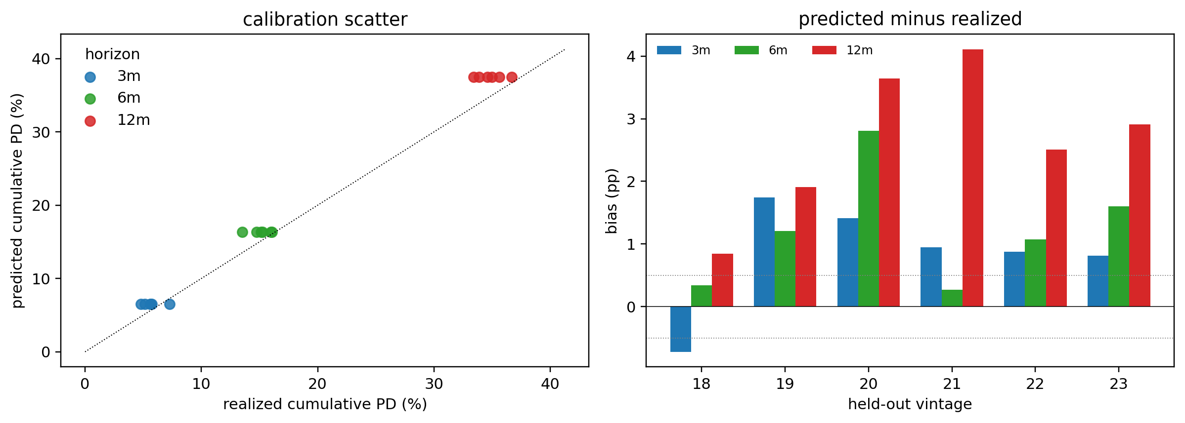
---
execute:
echo: true
eval: true
warning: false
message: false
bibliography:
- ../references.bib
- ../refs/ch-09.bib
---
# Survival Analysis and Time-to-Default {#sec-ch09}
::: {.callout-note appearance="simple" icon="false"}
**Scope: both retail and corporate.** Survival and discrete-time hazard models. Retail vintage analysis (account-level time-to-default) and corporate firm-year hazards (@sec-ch09-shumway, popularized by Shumway 2001) share the same likelihood.
:::
## Overview {.unnumbered}
### A failure that motivates the chapter {.unnumbered}
A logistic regression trained on a 36-month auto-loan vintage at month 6 and scored at month 24 will mis-rank an obligor who defaulted in month 4 the same way it mis-ranks one who was censored in month 4: both look like a positive label at horizon 6 even though the first obligor exited the risk set and the second is still on book. Dropping censored observations biases the bad rate; keeping them as zeros biases it the other way. Either way the IFRS 9 stage-2 lifetime provision computed off the resulting score is wrong by tens of basis points (the direction depends on which censoring choice you made), and the Basel one-year through-the-cycle PD is mis-calibrated by enough to fail an SR 11-7 effective-challenge benchmark against any model that respects the time axis. The failure is structural: a binary classifier *cannot* represent the joint distribution of (event, time) that the regulator's question is asking about. It is also avoidable: the same data, rescored on a Cox PH or a discrete-time Shumway logit fit on the same loan-month panel, recovers the time-dependent AUC and lifts the calibration deviation at 24 months back inside the stage-2 SLA. The rest of the chapter is what that rescoring entails, what it costs, and how to defend it in writing to four regulators.
A binary default flag tells you whether a loan went bad. It does not tell you when. In consumer and corporate credit, the when matters at least as much as the whether. A loan that defaults in month 6 bleeds capital differently from a loan that defaults in month 36. An IFRS 9 stage-2 provision [@ifrs9] depends on the lifetime distribution of default, not on a point prediction. A Basel IRB model [@basel2006international] must deliver a through-the-cycle probability of default at a one-year horizon, plus term-structure inputs for stress tests [@bellotti2013forecasting]. The problem is intrinsically temporal, and treating it as classification throws away the most useful piece of the data: the time axis.
Survival analysis is the right tool. It was built in biostatistics [@kaplan1958nonparametric; @cox1972regression; @aalen1978nonparametric] to handle exactly the situation lenders face: the event of interest may not occur during the observation window (censoring), covariates influence the timing of the event (regression on times), and competing events can preempt the one you care about (prepayment terminates a loan without default). Retail credit adopted these methods early [@narain1992survival; @banasik1999not; @stepanova2002survival] and continues to refine them [@bellotti2009credit; @dirick2017time].
### The chapter's throughline {.unnumbered}
Default is a time-to-event problem with five structural assumptions a model can lock in: independence of censoring from the event clock, a parametric (or nonparametric) hazard shape, proportional hazards across covariates, a single absorbing event, no immune fraction, and homogeneity within an observed risk band. This chapter walks the family of estimators that progressively relaxes those assumptions, scores the cost of each relaxation under controlled stress, and lands the surviving roster on a regulator-grade Vietnamese consumer-credit case study where four of the five assumptions are violated at once.
### Three threads, one chapter {.unnumbered}
The chapter braids three threads. Knowing which one you are on at any moment is the difference between reading the chapter and being lost in it.
- **Thread M (methods).** The genealogy walk from Kaplan-Meier down each branch (Cox, AFT, competing risks, cure, the heterogeneity extensions, Shumway). Every method section opens with the credit question it answers and the limitation of the prior section that motivated it. This is the chapter's spine.
- **Thread P (production).** Every method has a "leave the notebook" companion: the `survival_diagnostics` package (@sec-ch09-defensibility-production), the `discrete_hazard` package (@sec-ch09-shumway-production), the FastAPI scoring service (@sec-ch09-deployment), the MLflow artifact lineage, the Spark-scale fits (@sec-ch09-scalability). Each Thread P interlude opens with one paragraph on why the code needs to leave the notebook.
- **Thread C (case).** Two applied case threads do different work. The controlled six-DGP stress benchmark at @sec-ch09-comparison-stress proves the cost sheet at @sec-ch09-comparison-matrix by violating one assumption per world with a known oracle. The Vietnam capstone at @sec-ch09-vietnam-code proves the chapter on a portfolio that triggers four assumption violations at once with no oracle and a regulator watching.
### Reader contract {.unnumbered}
Three concrete promises:
- *Methods reader.* Every model is implemented twice (from-scratch so the math is visible, and with a reference library: `lifelines`, `scikit-survival`, `statsmodels`). Every section opens with the credit question it answers and the prior-section limitation it relaxes.
- *Production reader.* Every method has a Thread P interlude with a versioned package, a schema validator, a FastAPI surface, and an MLflow lineage. The cross-cutting infrastructure is gathered around @sec-ch09-deployment.
- *Reviewer reader.* The chapter delivers a cost sheet (@sec-ch09-comparison-matrix), a routing aid (@sec-ch09-comparison-flowchart), an upgrade aid (@sec-ch09-marketing's extension selector), a controlled assumption-violation oracle (@sec-ch09-comparison-stress), and a no-oracle public-file reality check (@sec-ch09-benchmark), all calibrated against a regulator's pre-read.
The case for survival models is sharpest in emerging markets. Vietnamese consumer loans book with thin CIC histories, cash-flow incomes that flex with Tet, and informal-sector obligors whose default timing concentrates in months 2 to 6 when a seasonal cash buffer runs out. A one-year classification target hides both the seasonal spike and the early-prepayment culture that ends the risk window for a large fraction of the book. The capstone case study at @sec-ch09-vietnam returns to this with Circular 11/2021 default timing, competing-risk prepayment from Tet bonuses, vintage analysis under macro volatility, and Decree 13/2023 data-protection obligations.
This chapter develops the machinery, end to end, from nonparametric product-limit estimators (@sec-ch09-km-cox) to parametric accelerated failure time models (@sec-ch09-aft), through competing risks (@sec-ch09-competing), cure mixtures (@sec-ch09-cure), heterogeneity and state dependence (@sec-ch09-marketing), vintage analysis (@sec-ch09-vintage), and the discrete-time hazard formulation (@sec-ch09-shumway) popularized in corporate default by @shumway2001forecasting and @duffie2007multi.
### Model genealogy: what each step up buys you {.unnumbered}
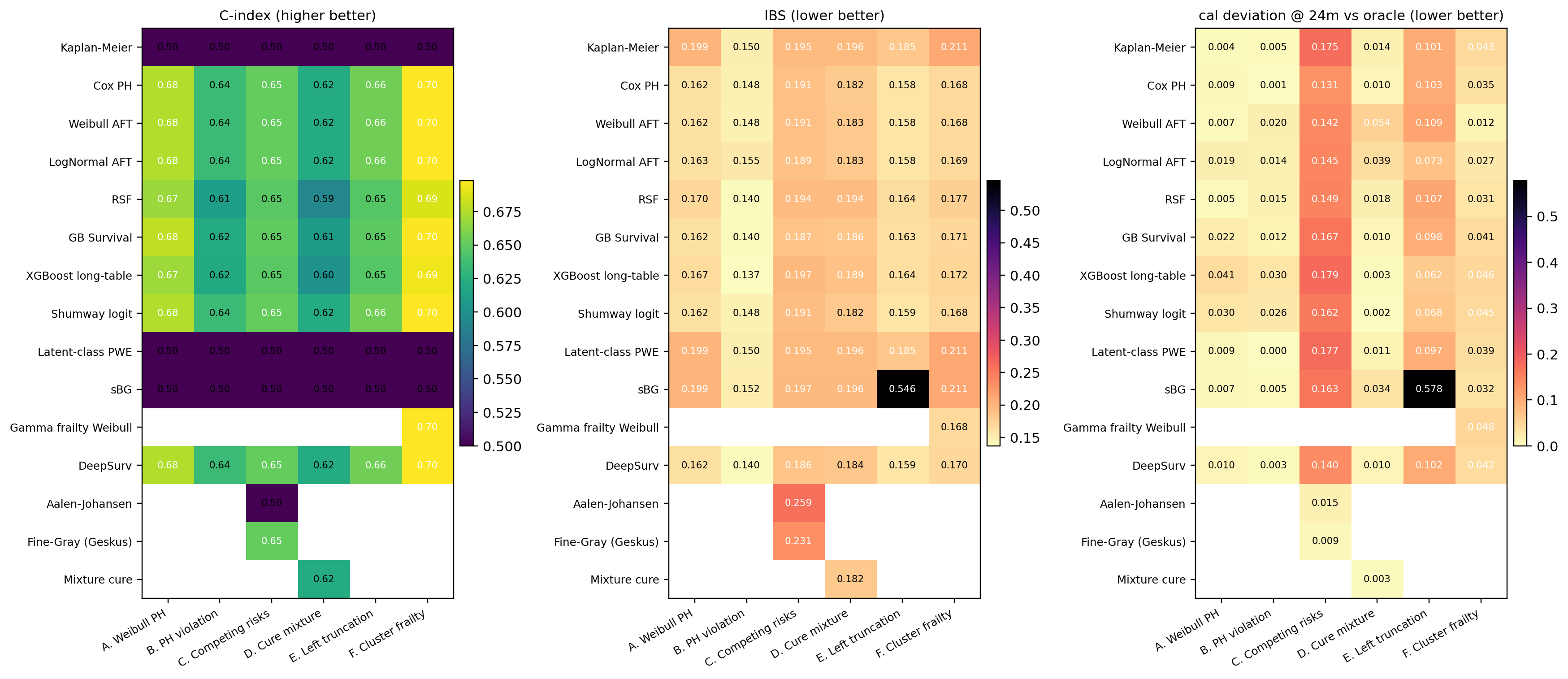
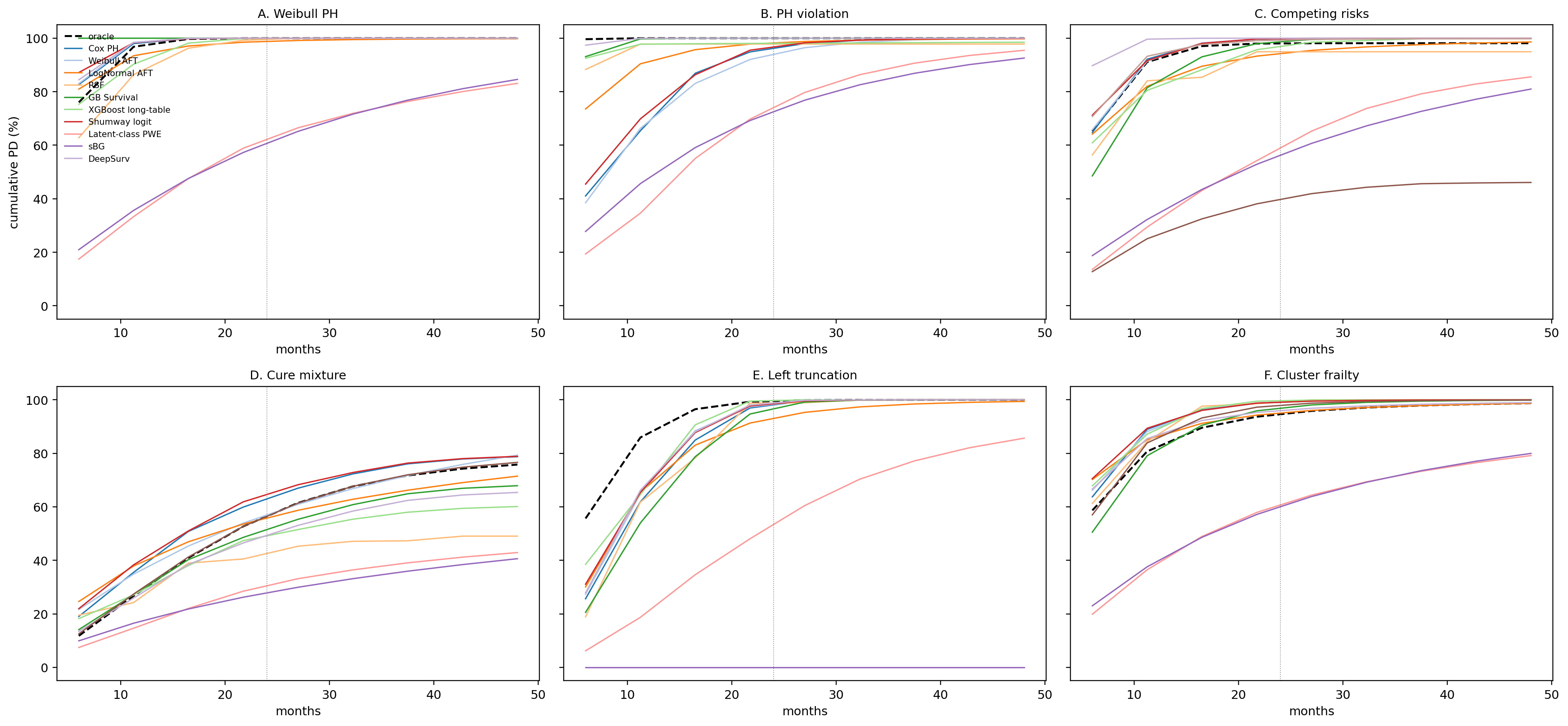
Survival is a family of models, not a single estimator. Each member of the family relaxes a structural assumption that an earlier member relied on, and pays for that flexibility somewhere else (more data, more compute, weaker extrapolation, harder identification). @fig-ch09-genealogy is the chapter map. The cost sheet at @sec-ch09-comparison-matrix is the dual: each row is a node on the tree, each column an assumption an arrow into the node relaxed. The routing aid at @sec-ch09-comparison-flowchart compresses both into binary questions a model-risk pre-read answers in five minutes. The stress benchmark at @sec-ch09-comparison-stress drops the whole roster onto six controlled DGPs and turns each cost-sheet entry into a number.
```{mermaid}
%%| label: fig-ch09-genealogy
%%| fig-cap: "Survival model genealogy. Each arrow is labeled with the assumption a more sophisticated estimator relaxes relative to its parent. Grey: anti-pattern baseline (binary classifier discards the time axis). Blue: regression backbones (Cox, AFT, Shumway). Orange: structure relaxers that add unobserved heterogeneity, immunity, or fully nonparametric hazard shape. Green: competing-risk estimators that admit more than one terminating event. Purple: marketing-style retention. The right way to read this chapter is to walk the tree from a question (extrapolate past observed horizon? cluster effect? immune fraction? competing prepayment?) to the cheapest family that answers yes."
graph TD
    BIN["Binary classifier<br/>(anti-pattern: discards 'when')"]
    KM["Kaplan-Meier<br/>marginal S(t)"]
    COX["Cox PH<br/>+ covariates (log-linear)"]
    STR["Cox + strata<br/>baseline varies across groups"]
    TVC["Cox + TVC<br/>covariates evolve over time"]
    FR["Frailty Cox / Weibull<br/>+ unobserved cluster effect"]
    AFT["AFT family<br/>(Weibull, LogNormal, LogLogistic)"]
    CURE["Mixture cure<br/>+ immune fraction"]
    AJ["Aalen-Johansen<br/>marginal CIF, multi-state"]
    FG["Fine-Gray<br/>covariates on CIF"]
    SHUM["Shumway discrete logit<br/>period basis, easy TVC"]
    LCPWE["Latent-class PWE<br/>+ discrete heterogeneity"]
    SBG["Shifted Beta-Geometric<br/>retention with beta heterogeneity"]
    RSF["RSF / GBSurv<br/>tree-based, free hazard shape"]
    DEEP["DeepSurv / XGB long-table<br/>scale to high-dim covariates"]

    BIN -->|"+ time axis, + censoring"| KM
    KM -->|"+ covariates (PH assumed)"| COX
    KM -->|"+ parametric shape → lifetime PD"| AFT
    KM -->|"+ competing event"| AJ
    KM -->|"+ geometric retention + heterogeneity"| SBG
    COX -->|"baseline per group"| STR
    COX -->|"covariates change over time"| TVC
    COX -->|"+ random effect on hazard"| FR
    COX -->|"discretize time, fit as logit"| SHUM
    COX -->|"drop log-linear, drop PH"| RSF
    COX -->|"drop log-linear, scale up"| DEEP
    AFT -->|"+ susceptible vs immune split"| CURE
    AJ -->|"+ covariates on subdistribution"| FG
    SHUM -->|"+ latent classes on hazard"| LCPWE

    classDef base fill:#f4f4f8,stroke:#444,color:#111;
    classDef regr fill:#eef3ff,stroke:#3355aa,color:#111;
    classDef relax fill:#fff1d6,stroke:#b8860b,color:#111;
    classDef compete fill:#e6f5ea,stroke:#2a8,color:#111;
    classDef retain fill:#f0e6f7,stroke:#7a3ea1,color:#111;
    class BIN,KM base;
    class COX,STR,TVC,AFT,SHUM regr;
    class FR,CURE,LCPWE,RSF,DEEP relax;
    class AJ,FG compete;
    class SBG retain;
```
A reader can use the map as a decision aid. *Need a one-year PD with the strongest discrimination on the file you have?* Walk down to RSF or GBSurv and accept that you cannot extrapolate past the longest training horizon. *Need a lifetime ECL curve to month 60 from a book observed only to month 36?* Walk down the AFT branch and pay with a parametric hazard shape. *Need a CIF that does not double-count prepayments as defaults?* Walk down to Aalen-Johansen, then to Fine-Gray once covariates matter. *Need a covariate effect that flips sign at age 12?* Walk down to TVC or to Shumway with a period basis. *Suspect a long-run immune fraction (revolvers who never default)?* Walk to mixture cure. *Suspect cluster heterogeneity (branches, dealers, originators)?* Walk to frailty Cox, or to latent-class PWE if the heterogeneity is discrete and the hazard shape is unknown. The chapter walks each branch, fits each model both from scratch and with a reference library, and closes at @sec-ch09-comparison with the same roster scored on six DGPs that each break exactly one assumption.
### Notation {.unnumbered}
- $T \in (0, \infty)$: time to default, a nonnegative random variable with density $f(t)$ and c.d.f. $F(t)$.
- $S(t) = \Pr(T > t) = 1 - F(t)$: survival function.
- $h(t) = \lim_{\Delta \downarrow 0} \Pr(t \le T < t+\Delta \mid T \ge t)/\Delta = f(t)/S(t)$: hazard rate.
- $H(t) = \int_0^t h(u)du = -\log S(t)$: cumulative hazard.
- $C$: right-censoring time, often administrative. We observe $Y = \min(T, C)$ and $\delta = \mathbf{1}\{T \le C\}$ (true default time seen), while $\delta= 0$: censored ($T >C$) (Loan still alive at cutoff $C$; default time unknown, only know $T > C$).
- $x \in \mathbb{R}^p$: time-fixed covariates (e.g., application attributes). $x(t)$: time-varying (e.g., unemployment rate in month $t$).
- $\beta \in \mathbb{R}^p$: regression coefficients in proportional hazards or AFT form.
- Vintage $v$: the origination period of a cohort. Age $a$: months since origination. Calendar $c = v + a$.
## Credit as survival {#sec-ch09-survival}
The logistic-regression failure that opened the chapter was a structural mismatch between the question (lifetime distribution of an event time) and the model (one-period probability of a binary label). The next page gives that question its language: a state machine for the loan, a likelihood that respects censoring, and three fundamental functions ($S$, $h$, $H$) that every estimator in the rest of the chapter is a parametrization of. Everything below in this section is data-side: shape of the panel, threats to identification, defensibility diagnostics. Everything from @sec-ch09-km-cox onward is a parametric or nonparametric specification of the hazard.
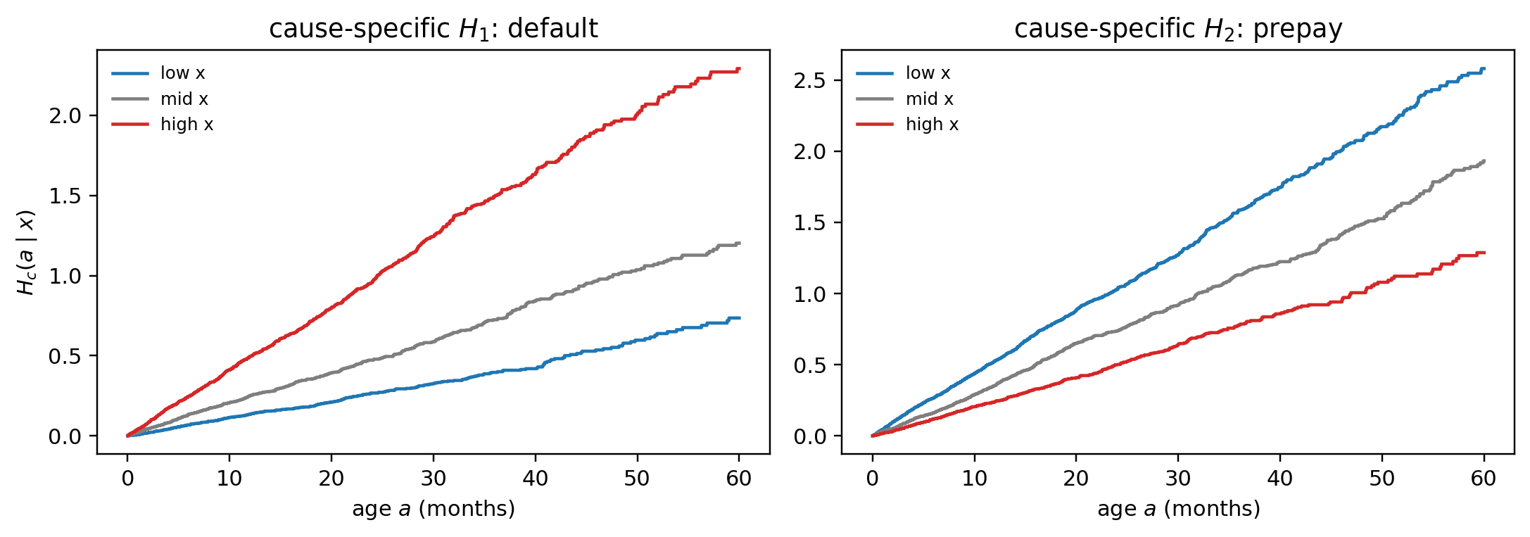
A loan originated in month $v$ with principal $L$ and contractual term $M$ becomes a point in a state diagram. At each month $a = 1, 2, \ldots, M$ the loan is in exactly one of four states: current, delinquent, defaulted, closed (paid off, refinanced, or written off). The transition of interest is current-or-delinquent to defaulted. Call that random transition time $T$. Because the loan matures at month $M$, the event time is right-censored at $C = M$ unless the loan prepays, in which case a competing event removes the loan from the risk set early. This is the canonical survival setup [@cox1972regression; @prentice1978analysis]. @fig-ch09-states draws the state machine: solid arrows are within-loan rolls, the bold arrow into *Defaulted* is the event of interest, *Closed* is the competing event, and reaching age $M$ without either is administrative right-censoring.
```{mermaid}
%%| label: fig-ch09-states
%%| fig-cap: "Loan-month state diagram. Each month the loan occupies exactly one node. *Current* and *Delinquent* form the at-risk set; the bold transition to *Defaulted* is the survival event $T$. *Closed* (prepay, refinance, write-off short of default) is a competing event that removes the loan from the risk set. Reaching contractual maturity $a=M$ without default or closure is administrative right-censoring at $C=M$."
stateDiagram-v2
    direction LR
    [*] --> Current: origination a=0
    Current --> Delinquent: miss payment
    Delinquent --> Current: cure
    Delinquent --> Defaulted: 90+ DPD, event T
    Current --> Closed: prepay or refinance
    Delinquent --> Closed: write-off or settlement
    Current --> Censored: reach maturity a=M
    Delinquent --> Censored: reach maturity a=M
    Defaulted --> [*]
    Closed --> [*]
    Censored --> [*]

    classDef risk fill:#eef3ff,stroke:#3355aa,color:#111;
    classDef event fill:#fde2e2,stroke:#a33,color:#111,font-weight:bold;
    classDef compete fill:#f4f4f8,stroke:#444,color:#111;
    classDef cens fill:#eafaf1,stroke:#2a8,color:#111;
    class Current,Delinquent risk;
    class Defaulted event;
    class Closed compete;
    class Censored cens;
```
The three fundamental functions are equivalent descriptions of the same distribution:
$$
S(t) = \Pr(T > t) = \exp\{-H(t)\}, \qquad H(t) = \int_0^t h(u) du, \qquad h(t) = -\frac{d}{dt}\log S(t).
$$ {#eq-triplet}
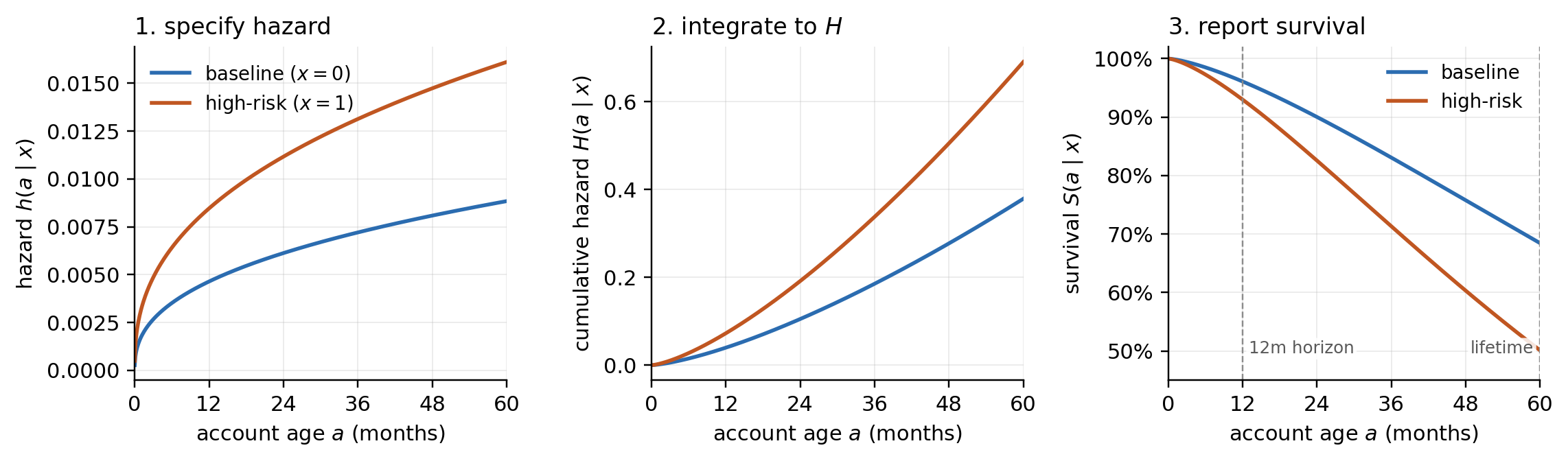
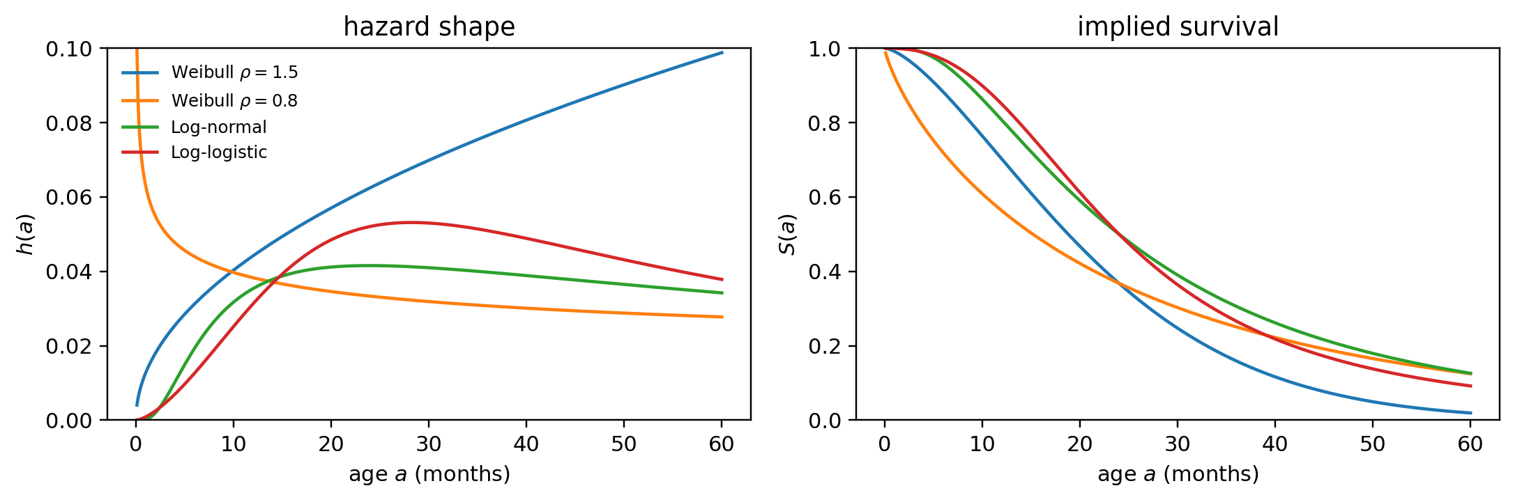
The hazard is the natural modeling primitive. It is local in time (unlike $S$ or $F$, which are cumulative), it is nonnegative (unlike derivatives of $F$, which are nonnegative only because $F$ is monotone), and covariates enter it in clean multiplicative or additive form. Credit risk measurement reports prefer $S(t)$ or the probability of default curve $F(t)$ because provisioning formulas, Basel risk-weight functions [@basel2017finalising], and stress tests quote lifetime or 12-month probabilities. A good modeler specifies $h$ and reports $S$. @fig-ch09-spec-report makes that workflow concrete: pick a parametric hazard, integrate to the cumulative hazard $H$, exponentiate to $S$, and read off the 12-month and lifetime PDs the report consumer actually wants.
### Right censoring and the likelihood
Right censoring is the defining feature of survival data. In retail credit, the most common form is administrative: the observation window ends at calendar time $\tau_{\text{end}}$, so a loan originated in month $v$ has follow-up $\tau_{\text{end}} - v$. Loans still current at $\tau_{\text{end}}$ contribute only their realized duration, not their (unobserved) default time.
Assume independent censoring: $T \perp C \mid x$. In words, among loans that share the same covariate vector $x$, the ones whose follow-up gets cut short carry no extra information about default timing beyond what their $x$ already says. Equivalently, the censoring mechanism is allowed to depend on $x$ (and on calendar time, since that is the same for everyone) but not on the latent $T$ once $x$ is conditioned on. If the assumption holds, the at-risk set $\mathcal{R}(t) = \{i : Y_i \ge t\}$ is a random sample of the population still at risk at age $t$, and the partial-likelihood and product-limit estimators treat each censored observation as "alive on its last seen day, future unknown" without bias.
Is the assumption realistic in retail credit? It is partly enforced by design and partly violated in practice. Three patterns matter:
1. *Administrative cutoff at* $\tau_{\text{end}}$ is the safe case. The data extraction date is exogenous to any individual loan's risk. Conditional on origination month $v$ and the covariate vector, the censoring time $C = \tau_{\text{end}} - v$ is deterministic, so $T \perp C \mid x, v$ holds by construction. This is why most credit-survival papers simply state "all censoring is administrative" and stop there.[^09-survival-analysis-1]
2. *Prepayment is the dangerous case.* A 36-month auto loan booked at month $v$ with covariates $x$ has a latent default time $T$ drawn from $h(t \mid x)$. At month 18, the borrower's credit improves (a fact not in $x$, unless you instrument refreshed scores), and a competitor offers a lower rate; the borrower refinances, so the loan is closed at $C = 18$ with $\delta_i = 0$. The naive likelihood treats this row as "survived 18 months, future unknown, average risk going forward" via the $S(18 \mid x)$ factor in @eq-liki. But the row was *not* average: it was a future low-risk borrower, removed from the risk set precisely because that information leaked through the refinance offer. Multiply across thousands of similar prepayments. After month 18, the surviving cohort is enriched in high-risk borrowers, the Kaplan-Meier drop rate over each subsequent interval rises, and the estimated baseline hazard $\hat{h}(t)$ for $t > 18$ tilts upward. Lifetime $\hat{F}(M \mid x) = 1 - \hat{S}(M \mid x)$ inherits the bias and the bank over-reserves on a portfolio that, if anything, is healthier than reported. **Fix**: do not call refinance "censoring." Treat it as a competing event with its own cause-specific hazard $h_{\text{prepay}}(t \mid x)$, fit jointly, and use Aalen-Johansen or Fine-Gray for the report (see @sec-ch09-competing).
3. *Lender-initiated closure (line cuts, charge-off short of default, forced refinance) is the intermediate case.* The decision is made by the bank using information about the account that may or may not be in $x$. If risk-driver scores, behavior, and macro covariates are all in $x$, conditional independence is plausible; if not, censoring is informative.[^09-survival-analysis-2]
[^09-survival-analysis-1]: Even the safe case has corner cases. Suppose the bank truncates the data extract at $\tau_{\text{end}}$ but a separate IT pipeline drops loans that have been "inactive" for three months ahead of extraction. Now $C$ depends on payment behavior, which depends on $T$. The fix is to use the original servicing snapshot, not a cleaned downstream copy.
[^09-survival-analysis-2]: Three concrete examples. (a) *Hardship programs* in the 2020 pandemic re-amortized millions of mortgages. The eligibility rule (recent unemployment, payment hardship attestation) used information about the borrower that the application-time $x$ did not contain. Loans that entered hardship were closed in the analytic record at the modification date; they were the ones most likely to default. Treating them as censored biases the default hazard *down*. (b) *Credit-line reductions* on revolving products. The bank cuts the limit on accounts whose utilization is climbing or whose external bureau score has fallen, and the account either pays out or transitions to a different product, ending its observation. Censoring depends on a behavior covariate that is rarely in the application-time $x$. (c) *Dealer recourse on indirect auto loans.* Loans bought with recourse can be sold back to the dealer when the dealer suspects payment trouble; those exits look like prepayments in the servicer's record but track future default better than prepayment does.
Independent censoring is *not* fully testable from observed data: $T$ is unobserved precisely when $C$ is observed, so the joint distribution $(T, C)$ is not identified without further assumptions [@tsiatis1975nonidentifiability]. What can be done is to gather evidence:
- *Compare covariate distributions across censoring causes.* If administratively-censored loans, prepaid loans, and lender-closed loans have visibly different $x$ distributions, conditional independence is more demanding; either widen $x$ or model the cause explicitly.
- *Inverse-probability-of-censoring weighting (IPCW).* Fit a model for the censoring hazard $\lambda_C(t \mid x)$, weight each at-risk observation by $1/\hat{S}_C(t \mid x)$, and refit the survival model. Stable estimates under IPCW are evidence that conditional independence on the chosen $x$ is enough; large shifts say the censoring depends on something not in $x$ [@robins1992recovery].
- *Sensitivity / tipping-point analysis.* Assume censored borrowers default at rate $\rho \cdot \hat{h}(t \mid x)$ for $\rho \in [0.5, 2]$ and re-estimate $S$. Report the range. If the 12m PD is stable across the range, the report is robust; if it flips sign on a key decision, escalate.
- *Holdout against a clean cohort.* Where possible, fit on a vintage with mostly administrative censoring and compare the implied hazard to a vintage with heavy prepay. Persistent disagreement past what covariates explain is informative-censoring evidence.
> $T \perp C \mid x$ is a working assumption that you make defensible by
>
> \(a\) including the covariates that drive censoring,
>
> \(b\) modeling prepayment as a competing event rather than independent censoring, and
>
> \(c\) reporting the IPCW or tipping-point sensitivity alongside the headline survival curve.
>
> @sec-ch09-defensibility runs all four diagnostics in code on the simulated cohort.
Then the contribution of observation $i$ to the likelihood is
$$
\begin{aligned}
L_i(\theta) &= f(y_i \mid x_i; \theta)^{\delta_i}\, S(y_i \mid x_i; \theta)^{1-\delta_i} \\
&= \bigl[h(y_i \mid x_i; \theta)\, S(y_i \mid x_i; \theta)\bigr]^{\delta_i}\, S(y_i \mid x_i; \theta)^{1-\delta_i} \\
&= h(y_i \mid x_i; \theta)^{\delta_i}\, S(y_i \mid x_i; \theta)^{\delta_i + (1-\delta_i)} \\
&= h(y_i \mid x_i; \theta)^{\delta_i}\, S(y_i \mid x_i; \theta).
\end{aligned}
$$ {#eq-liki}
The step from line one to line two is the key substitution: $f(t) = h(t)\, S(t)$. This follows immediately from the definition of the hazard, $h(t) = f(t)/S(t)$, just rearranged. Once both observed and censored contributions are written in terms of $h$ and $S$, they share the same survival factor and the powers of $S$ collapse from $\delta_i + (1 - \delta_i) = 1$ to a single $S(y_i \mid x_i; \theta)$. The remaining $h^{\delta_i}$ rewards the model only when an event was actually observed ($\delta_i = 1$), and is silent otherwise. This is exactly why the hazard, not the density, is the natural primitive to specify: censored rows contribute through $S$, event rows contribute through $h \cdot S$, and both terms are something the modeler already controls.
Total log-likelihood is $\ell(\theta) = \sum_i \delta_i \log h(y_i \mid x_i; \theta) - H(y_i \mid x_i; \theta)$. Every parametric model we will fit in this chapter (Weibull, log-logistic, log-normal, Cox with Breslow baseline, mixture cure) is a special case of @eq-liki. Every likelihood-ratio test, AIC comparison, and Wald statistic derives from it.
A related but distinct pitfall is *left truncation*. Suppose the analytic window opens at calendar time $\tau_{\text{start}}$ and a loan was originated earlier, at $v < \tau_{\text{start}}$. The loan only enters the dataset because it was *still alive* at $\tau_{\text{start}}$, that is, at age $a_0 = \tau_{\text{start}} - v > 0$. What is wrong with treating it as if it had been observed from age 0? Two things, both about selection.
- First, the cohort of "loans alive at $\tau_{\text{start}}$" excludes every loan from the same vintage that already defaulted before $\tau_{\text{start}}$. Pretending the observation started at age 0 puts a survivor in the risk set at every young age $0 \le t < a_0$ where they were *not actually observable*, so $n_k$ in the KM denominator is inflated for early time bins. Early hazards come out biased *downward*.
- Second, the at-risk indicator inside the partial likelihood becomes wrong: at event time $t < a_0$, this loan should not be in $\mathcal{R}(t)$ at all, because we would never have seen it had it failed before $\tau_{\text{start}}$. Including it pretends we had information we did not.
The fix is *delayed entry*, not deletion. Drop the rows and you discard valid follow-up at ages $a \ge a_0$, throwing away exactly the data the older vintages contribute (and biasing toward young vintages, which themselves bias toward early defaulters). Instead, re-define each row's at-risk window: enter the risk set at age $a_0$, exit at age $a_0 + \text{follow-up}$, with the event indicator unchanged. The Kaplan-Meier and Cox estimators then form $\mathcal{R}(t) = \{i : a_0^{(i)} \le t \le \text{exit}^{(i)}\}$ and the math goes through. The `lifelines` `entry` argument and the counting-process $(\text{start}, \text{stop}, \text{event})$ formulation of @andersen1982cox implement this directly. @sec-ch09-truncation-demo shows the bias and the fix on simulated data.
The mirror-image pitfall is *right truncation*. It is structurally distinct from right *censoring* and the two are routinely confused in the credit-risk literature. Right censoring means a loan is alive at the analysis cutoff and we will eventually see whether it defaults; the row is in the dataset, the event time is bounded below. Right truncation means the row is in the dataset *only because* the event has already happened by some calendar bound. Three concrete sources in production:
- *Defaulted-only extracts.* The data team hands you a chargeoff table joined to origination, on the grounds that "good loans don't need a default-time field". Every row is a defaulter; the never-defaulted population is silently absent.
- *Reporting-lag truncation in incident data.* Fraud, first-payment-default, or recovery feeds arrive at the warehouse only once a case file is closed. The cohort assembled at calendar time $\tau_{\text{end}}$ contains case $i$ iff $t_{\text{event}}^{(i)} + \ell^{(i)} \le \tau_{\text{end}}$, where $\ell$ is the random reporting lag. Long-lag events for recently-originated loans are not yet visible.
- *Recovery-time studies.* Loss-given-default analyses that retain only loans whose recovery completed by $\tau_{\text{end}}$ truncate exactly the long-lag, low-recovery tail.
Naively fitting Kaplan-Meier on a right-truncated sample biases the survival curve *upward at the tail* (long-failing loans are over-represented) and *downward at the head* (short-failing loans are over-represented relative to the full origination cohort). The standard fixes invert the time axis and run KM on $\tau - t$ [@lagakos1988nonparametric] or use the @efron1999nonparametric self-consistent NPMLE. In `lifelines` the practical handle is `KaplanMeierFitter.fit_left_truncation_right_censoring` for the symmetric case; for retrospective right-truncation only, the reverse-time KM is a half-page of NumPy. @sec-ch09-right-truncation-demo shows both the bias and the fix on simulated data, and `survival_diagnostics.truncation` ships a production guard that flags when an incoming cohort looks event-only.
### Why not just classification?
A naive approach frames default as a binary outcome: over the horizon $H$, did the borrower default? Fit a logistic regression [@thomas2000survey]. That works when $H$ is fixed and the portfolio composition is stable. It fails in three ways:
1. **Horizons are not fixed**. IFRS 9 stage-2 uses lifetime. Scenario testing uses 3-year. Pricing uses 5-year. A single logistic cannot produce all three without refitting.
2. **Censoring is ignored**. A loan booked 3 months ago with 33 months to go is treated as a non-default. It gives the same evidence as a loan that survived 36 months. The first is mostly missing.
3. **The time profile is informative**. Early defaults cluster around affordability shocks; late defaults track adverse selection and macro shocks [@duffie2007multi; @bellotti2009credit]. A hazard curve carries that signature.
The rest of the chapter shows how to extract it.
```{python}
#| label: setup
import sys
sys.path.insert(0, '../code')
import os
os.environ.setdefault('OMP_NUM_THREADS', '2')

import numpy as np
import pandas as pd
import matplotlib.pyplot as plt

rng = np.random.default_rng(7)
plt.rcParams.update({'figure.dpi': 110, 'savefig.bbox': 'tight'})
```
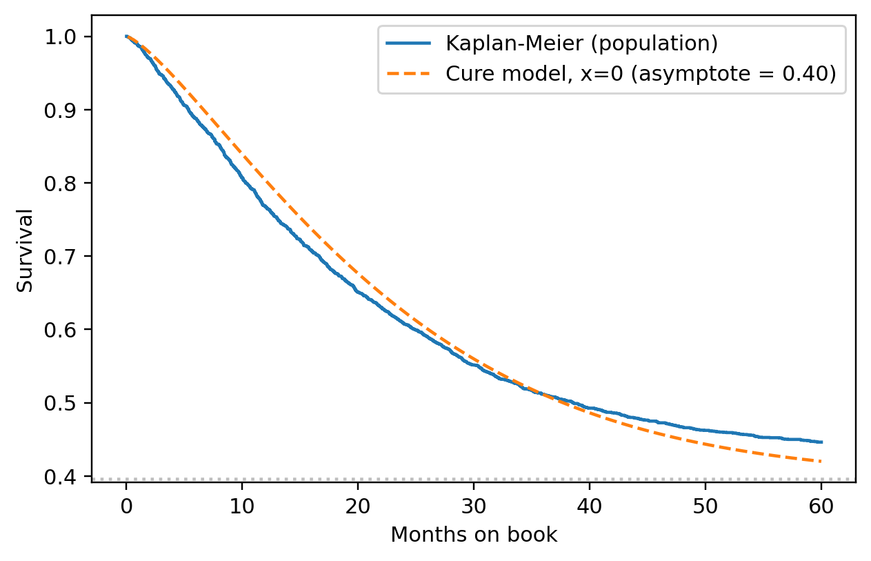
To make "specify $h$, report $S$" tangible before any data appears, fix a Weibull hazard $h(t \mid x) = (k/\lambda)(t/\lambda)^{k-1} \exp(\beta x)$ with shape $k$, scale $\lambda$, and a single binary covariate $x \in \{0, 1\}$ for a higher-risk segment. The modeler chooses the hazard form and parameters; everything the report consumer sees is derived. The cumulative hazard is $H(t \mid x) = (t/\lambda)^k \exp(\beta x)$, the survival is $S(t \mid x) = \exp\{-H(t \mid x)\}$, and the marginal default probability over horizon $H$ is $F(H \mid x) = 1 - S(H \mid x)$. @fig-ch09-spec-report shows the three curves; the table below it converts to the two numbers a stress test or IFRS 9 stage classifier actually wants.
```{python}
#| label: fig-ch09-spec-report
#| fig-cap: "Specify hazard, report survival. Left: parametric Weibull hazard $h(t \\mid x)$ for two segments (specified by the modeler, $k=1.4$, $\\lambda=120$ months, $\\beta=0.6$ for the high-risk flag). Middle: cumulative hazard $H(t \\mid x) = \\int_0^t h$. Right: survival $S(t \\mid x) = e^{-H}$, with vertical guides at the 12-month IFRS 9 stage-2 horizon and the 60-month contractual maturity. The reported numbers, 12m PD and lifetime PD, are read off the right panel."
k, lam = 1.4, 120.0
beta = 0.6
M = 60
t = np.linspace(0.01, M, 600)

def weibull_h(t, k, lam, x, beta):
    return (k / lam) * (t / lam) ** (k - 1) * np.exp(beta * x)

def weibull_H(t, k, lam, x, beta):
    return (t / lam) ** k * np.exp(beta * x)

h0 = weibull_h(t, k, lam, x=0, beta=beta)
h1 = weibull_h(t, k, lam, x=1, beta=beta)
H0, H1 = weibull_H(t, k, lam, 0, beta), weibull_H(t, k, lam, 1, beta)
S0, S1 = np.exp(-H0), np.exp(-H1)

c0, c1 = '#2b6cb0', '#c05621'
fig, ax = plt.subplots(1, 3, figsize=(10.5, 3.2), sharex=True)
for a in ax:
    a.grid(True, alpha=0.25, lw=0.6)
    for side in ('top', 'right'):
        a.spines[side].set_visible(False)
    a.set_xlabel('account age $a$ (months)')
    a.set_xlim(0, M)
    a.set_xticks([0, 12, 24, 36, 48, 60])

ax[0].plot(t, h0, color=c0, lw=1.8, label='baseline ($x=0$)')
ax[0].plot(t, h1, color=c1, lw=1.8, label='high-risk ($x=1$)')
ax[0].set_ylabel('hazard $h(a \\mid x)$')
ax[0].set_title('1. specify hazard', loc='left', fontsize=11)
ax[0].legend(frameon=False, loc='upper left', fontsize=9)

ax[1].plot(t, H0, color=c0, lw=1.8)
ax[1].plot(t, H1, color=c1, lw=1.8)
ax[1].set_ylabel('cumulative hazard $H(a \\mid x)$')
ax[1].set_title('2. integrate to $H$', loc='left', fontsize=11)

ax[2].plot(t, S0, color=c0, lw=1.8, label='baseline')
ax[2].plot(t, S1, color=c1, lw=1.8, label='high-risk')
ax[2].set_ylabel('survival $S(a \\mid x)$')
ax[2].set_title('3. report survival', loc='left', fontsize=11)
ax[2].set_ylim(0.45, 1.02)
ax[2].yaxis.set_major_formatter(plt.FuncFormatter(lambda v, _: f'{v:.0%}'))
for h_mark, lbl, ha, dx in [(12, '12m horizon', 'left', 1.0), (60, 'lifetime', 'right', -1.0)]:
    ax[2].axvline(h_mark, color='0.55', lw=0.8, ls='--')
    ax[2].text(h_mark + dx, 0.49, lbl, ha=ha, va='bottom',
               fontsize=8, color='0.35',
               bbox=dict(boxstyle='round,pad=0.15', fc='white', ec='none', alpha=0.85))
ax[2].legend(frameon=False, loc='upper right', fontsize=9)

fig.tight_layout()
plt.show()
```
```{python}
#| label: tbl-ch09-spec-report
report = pd.DataFrame({
    'segment': ['baseline (x=0)', 'high-risk (x=1)'],
    '12m PD': [1 - np.exp(-weibull_H(12, k, lam, 0, beta)),
               1 - np.exp(-weibull_H(12, k, lam, 1, beta))],
    'lifetime PD (M=60)': [1 - np.exp(-weibull_H(M, k, lam, 0, beta)),
                            1 - np.exp(-weibull_H(M, k, lam, 1, beta))],
})
report.round(4)
```
The modeler touched only $k$, $\lambda$, $\beta$. Everything the report shows, the curves and the two PDs, follows from @eq-triplet. Swapping the Weibull for a Cox baseline plus the same $\beta x$ would change the *shape* of $h$, but leave the pipeline (hazard $\to$ $H$ $\to$ $S$ $\to$ horizon PD) identical; that is the payoff of treating the hazard as the primitive. The remaining sections of this chapter populate the *specify* $h$ step with progressively richer estimators, but the *report* $S$ step never changes.
### Informative censoring: a numerical demo {#sec-ch09-informative-censoring-demo}
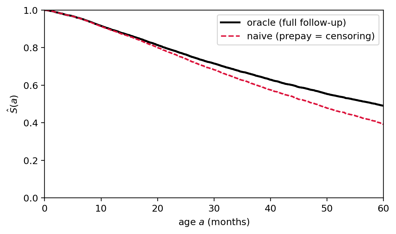
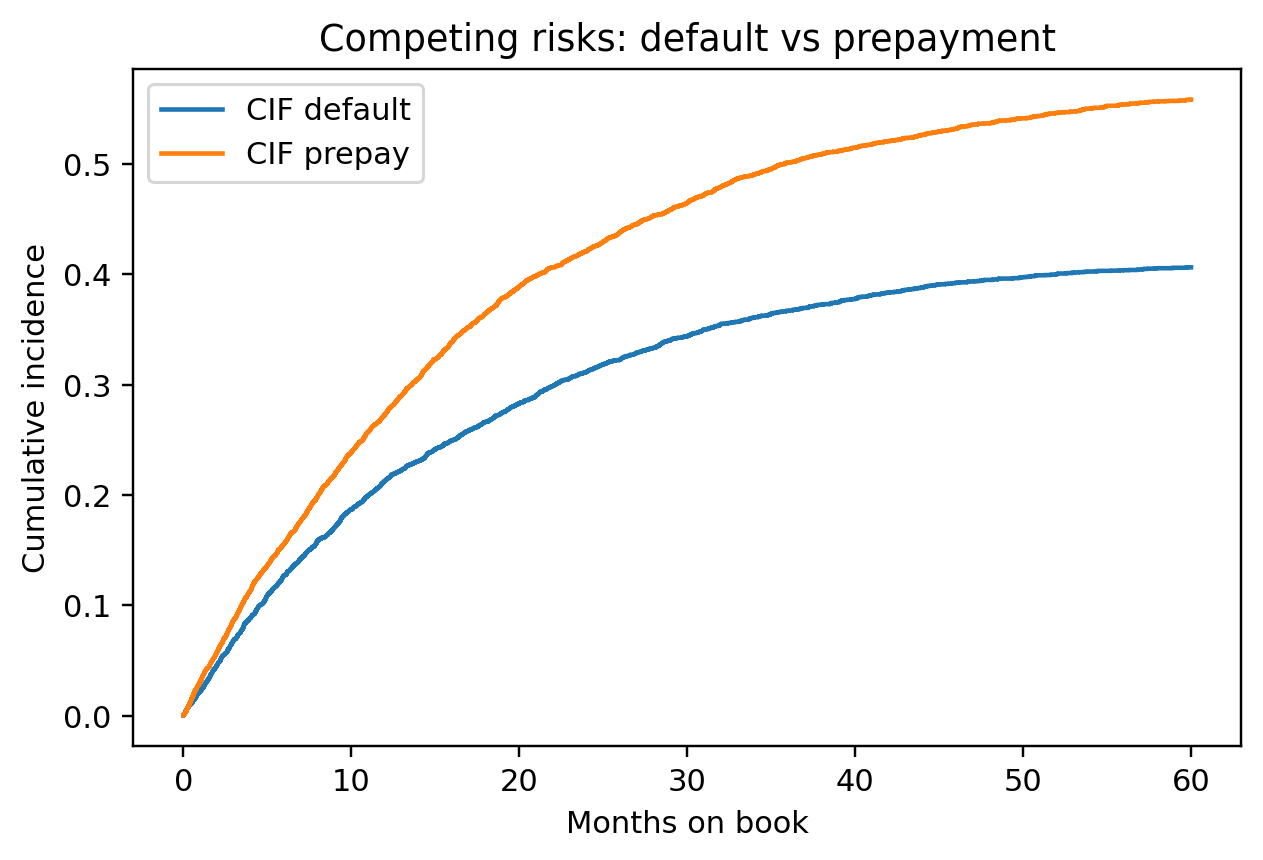
The earlier walkthrough claimed that treating prepayment as independent censoring biases the survival estimate. @fig-ch09-informative-censoring quantifies the bias on a simulated cohort where a latent risk score $Z$ drives both the default time and the prepayment time, in opposite directions: high $Z$ (bad risks) default early and rarely prepay; low $Z$ (good risks) survive long and prepay early. The naive Kaplan-Meier curve treats prepayments as ordinary censoring; the oracle curve uses the full latent default time. The gap is the bias.
```{python}
#| label: fig-ch09-informative-censoring
#| fig-cap: "Informative censoring from prepayment. Black: oracle Kaplan-Meier built from the latent default time $T$ followed for the full contractual term $M$. Red dashed: naive KM that treats prepayments as ordinary censoring on a cohort where good risks prepay early. The naive curve runs *below* the truth at later ages because, after the good risks leave, the surviving at-risk set is enriched in bad risks; the estimated drop rate per interval rises and survival is understated. Reverse the sign of the dependence and the bias flips."
from lifelines import KaplanMeierFitter

n = 6000
k_w, lam_base, alpha = 1.4, 80.0, 0.8
M_term = 60

Z = rng.normal(size=n)
T_lat = lam_base * np.exp(-alpha * Z) * rng.weibull(k_w, size=n)
P_lat = lam_base * np.exp(+alpha * Z) * rng.weibull(k_w, size=n)

Y = np.minimum.reduce([T_lat, P_lat, np.full(n, M_term)])
delta_naive = ((T_lat <= P_lat) & (T_lat <= M_term)).astype(int)

Y_oracle = np.minimum(T_lat, M_term)
delta_oracle = (T_lat <= M_term).astype(int)

kmf_truth = KaplanMeierFitter().fit(Y_oracle, delta_oracle, label='oracle (full follow-up)')
kmf_naive = KaplanMeierFitter().fit(Y, delta_naive, label='naive (prepay = censoring)')

fig, ax = plt.subplots(1, 1, figsize=(6.0, 3.6))
kmf_truth.plot_survival_function(ax=ax, ci_show=False, color='black', lw=2)
kmf_naive.plot_survival_function(ax=ax, ci_show=False, color='crimson', linestyle='--')
ax.set_xlabel('age $a$ (months)'); ax.set_ylabel('$\\hat S(a)$')
ax.set_xlim(0, M_term); ax.set_ylim(0, 1)
fig.tight_layout(); plt.show()

print(f"oracle 12m PD : {1 - float(kmf_truth.predict(12)):.4f}")
print(f"naive  12m PD : {1 - float(kmf_naive.predict(12)):.4f}")
print(f"oracle lifetime PD: {1 - float(kmf_truth.predict(M_term-1)):.4f}")
print(f"naive  lifetime PD: {1 - float(kmf_naive.predict(M_term-1)):.4f}")
```
The naive lifetime PD comes out larger than the truth: prepay-driven exits removed the good risks early, so the conditional default rate among the survivors is inflated. In a real portfolio you do not have the oracle column; the right move is to recognize prepay as a competing event (@sec-ch09-competing) and report cause-specific or Aalen-Johansen cumulative incidence instead of treating prepay as censoring.
### Defensibility diagnostics: IPCW, tipping-point, and cohort holdout {#sec-ch09-defensibility}
Independence $T \perp C \mid x$ is untestable directly: the joint distribution of $(T, C)$ is not identified from the data we observe. Four diagnostics provide *indirect* evidence by attacking the assumption from different angles. Each answers a distinct sub-question, and a validation pack should report all four:
1. *Cause-cohort overlap* asks whether censored loans look like at-risk loans on the covariates we already have.
2. *IPCW reweighting* asks whether putting the suspect covariate into the censoring model closes the bias.
3. *Tipping-point sensitivity* asks how wrong the assumption would have to be before the headline number flips.
4. *Clean-cohort holdout* asks whether the bias disappears on a parallel vintage where censoring is rare.
All four run on the cohort from @sec-ch09-informative-censoring-demo, so the bias in @fig-ch09-informative-censoring and its corrections share one axis. The output is the artifact a model-validation pack attaches next to the headline KM curve.
#### Diagnostic 1: cause-cohort overlap on covariates {#sec-ch09-defensibility-overlap}
**Question.** Do prepaid loans look like administratively-censored loans on the observed covariates?
**Intuition.** If censoring is unrelated to risk *conditional on* $x$, then censored and at-risk loans should share the same $x$ distribution within each stratum. The diagnostic is as follows: when prepaid loans cluster at low $Z$ (good risks), while admin-censored loans straddle the full $Z$ range, $x$ is too narrow to absorb the dependence. We do not need to know the truth to see this; we just need the cause-of-exit label.
**How to read it.** A Kolmogorov-Smirnov statistic on $Z$ across cause cohorts, plus group means and standard deviations. A large KS distance with a small p-value means censoring is selective on $Z$, which forces a choice: widen $x$ to include $Z$, or move to IPCW with $Z$ in the censoring model.
```{python}
#| label: tbl-ch09-cause-overlap
from scipy.stats import ks_2samp

cause = np.where(delta_naive == 1, 'default',
        np.where((P_lat <= T_lat) & (P_lat <= M_term), 'prepay', 'admin'))
cause_df = pd.DataFrame({'Z': Z, 'cause': cause})

summary = cause_df.groupby('cause')['Z'].agg(['count', 'mean', 'std']).round(3)
ks_admin_vs_prepay = ks_2samp(cause_df.query("cause=='admin'")['Z'],
                              cause_df.query("cause=='prepay'")['Z'])
ks_admin_vs_default = ks_2samp(cause_df.query("cause=='admin'")['Z'],
                               cause_df.query("cause=='default'")['Z'])
print(summary)
print(f"KS(admin vs prepay)  : D={ks_admin_vs_prepay.statistic:.3f}  p={ks_admin_vs_prepay.pvalue:.2e}")
print(f"KS(admin vs default) : D={ks_admin_vs_default.statistic:.3f}  p={ks_admin_vs_default.pvalue:.2e}")
```
The prepaid pool sits at low $Z$ (good risks), the default pool at high $Z$, and admin censoring straddles both because it conditions only on age. The KS distance between admin and prepay is large and the null of equal $Z$ distributions is rejected: the censoring mechanism *is* selective on $Z$.
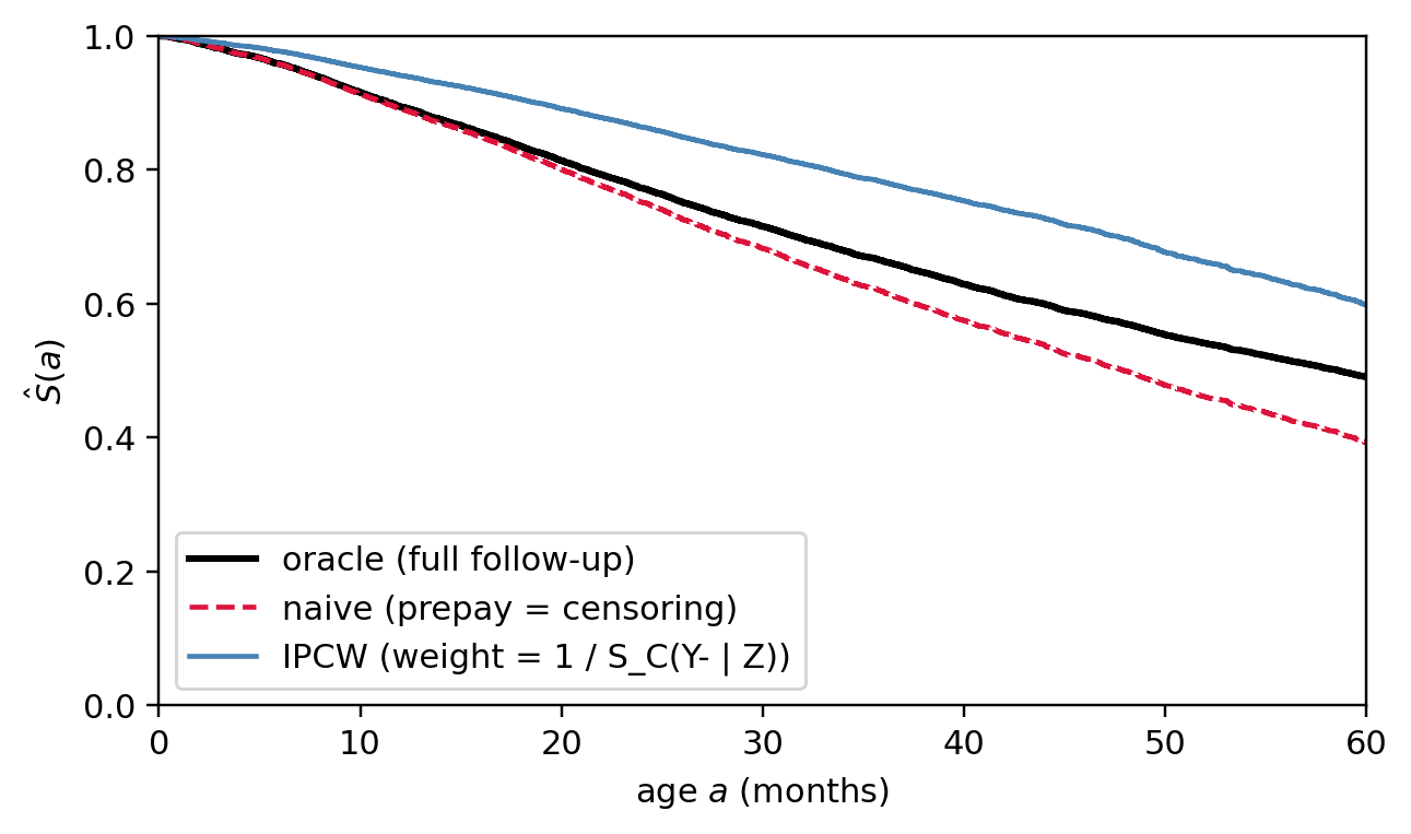
#### Diagnostic 2: IPCW reweighting {#sec-ch09-defensibility-ipcw}
**Question.** If we put the suspect covariate into the censoring model, does the bias close?
**Intuition.** Every loan that prepays would have continued accruing default-time information had it stayed in the book. IPCW reconstructs that lost information by *upweighting at-risk loans that look like the prepaid ones*, where resemblance is measured through the censoring survival $\hat S_C(Y_i^- \mid x_i)$ from a Cox model fit on the prepay hazard. Each row carries weight $1/\hat S_C$: observations whose covariate-siblings tend to leave early carry more weight, because they are speaking on behalf of the prepayers we no longer observe. If the lost information runs along $x$, IPCW recovers it; if it runs along an *unmeasured* driver, IPCW cannot help and the residual gap is evidence of that.
**How to read it.** Overlay three KMs: the oracle (latent $T$, no prepay), the naive (treats prepay as independent censoring), and the IPCW-weighted. A closed gap on the IPCW curve is a positive signal but not proof, since IPCW only corrects for marginalization across the modeled covariates. Watch the weights: a max or 99th-percentile weight past 5-10 means a handful of rows do most of the correcting and bootstrap CIs widen accordingly. Production stabilizes the weights (numerator $\hat S_C^{\text{marg}}(t)$ from a covariate-free censoring KM) and caps at the 99th percentile to trade a small bias for a large variance reduction; @robins1992recovery is the IPCW reference.
```{python}
#| label: fig-ch09-ipcw
#| fig-cap: "IPCW correction. Black: oracle KM (latent $T$, no prepay). Red dashed: naive KM that treats prepay as ordinary censoring and ignores $Z$. Blue: IPCW-weighted KM where each row carries weight $1/\\hat S_C(Y_i^- \\mid Z_i)$ from a Cox model for the prepay hazard. The IPCW curve closes most of the gap because the lost information runs along $Z$, which the censoring model captures. A residual gap survives because IPCW corrects for marginalisation, not for unmeasured drivers; if the gap stayed wide after conditioning on every observable, that would be evidence of unmeasured informative censoring."
from lifelines import CoxPHFitter

prep_df = pd.DataFrame({'Y': Y, 'event_def': delta_naive, 'Z': Z})
prep_df['event_prep'] = ((P_lat <= T_lat) & (P_lat <= M_term)).astype(int)

cph_C = CoxPHFitter(penalizer=1e-4).fit(prep_df[['Y', 'event_prep', 'Z']],
                                        duration_col='Y', event_col='event_prep')
times_sorted = np.unique(np.append(Y, [0.0]))
S_C = cph_C.predict_survival_function(prep_df[['Z']], times=times_sorted)
idx = np.searchsorted(times_sorted, Y, side='right') - 1
S_C_at_Y = np.clip(S_C.values[idx, np.arange(n)], 0.05, 1.0)
w_ipcw = 1.0 / S_C_at_Y

kmf_ipcw = KaplanMeierFitter().fit(Y, delta_naive, weights=w_ipcw,
                                   label='IPCW (weight = 1 / S_C(Y- | Z))')

fig, ax = plt.subplots(1, 1, figsize=(6.0, 3.6))
kmf_truth.plot_survival_function(ax=ax, ci_show=False, color='black', lw=2)
kmf_naive.plot_survival_function(ax=ax, ci_show=False, color='crimson', linestyle='--')
kmf_ipcw.plot_survival_function(ax=ax, ci_show=False, color='steelblue')
ax.set_xlabel('age $a$ (months)'); ax.set_ylabel('$\\hat S(a)$')
ax.set_xlim(0, M_term); ax.set_ylim(0, 1)
fig.tight_layout(); plt.show()

pd_oracle = 1 - float(kmf_truth.predict(12))
pd_naive  = 1 - float(kmf_naive.predict(12))
pd_ipcw   = 1 - float(kmf_ipcw.predict(12))
print(f"12m PD  oracle={pd_oracle:.4f}  naive={pd_naive:.4f}  IPCW={pd_ipcw:.4f}")
print(f"weight summary  min={w_ipcw.min():.2f}  median={np.median(w_ipcw):.2f}  "
      f"p99={np.quantile(w_ipcw, 0.99):.2f}  max={w_ipcw.max():.2f}")
```
The IPCW curve closes most of the gap on this cohort because the lost information runs along $Z$, which the censoring model captures. A residual gap survives because IPCW corrects for marginalisation, not for unmeasured drivers; if the gap stayed wide after conditioning on every observable, that would be evidence of unmeasured informative censoring and a job for Diagnostic 3.
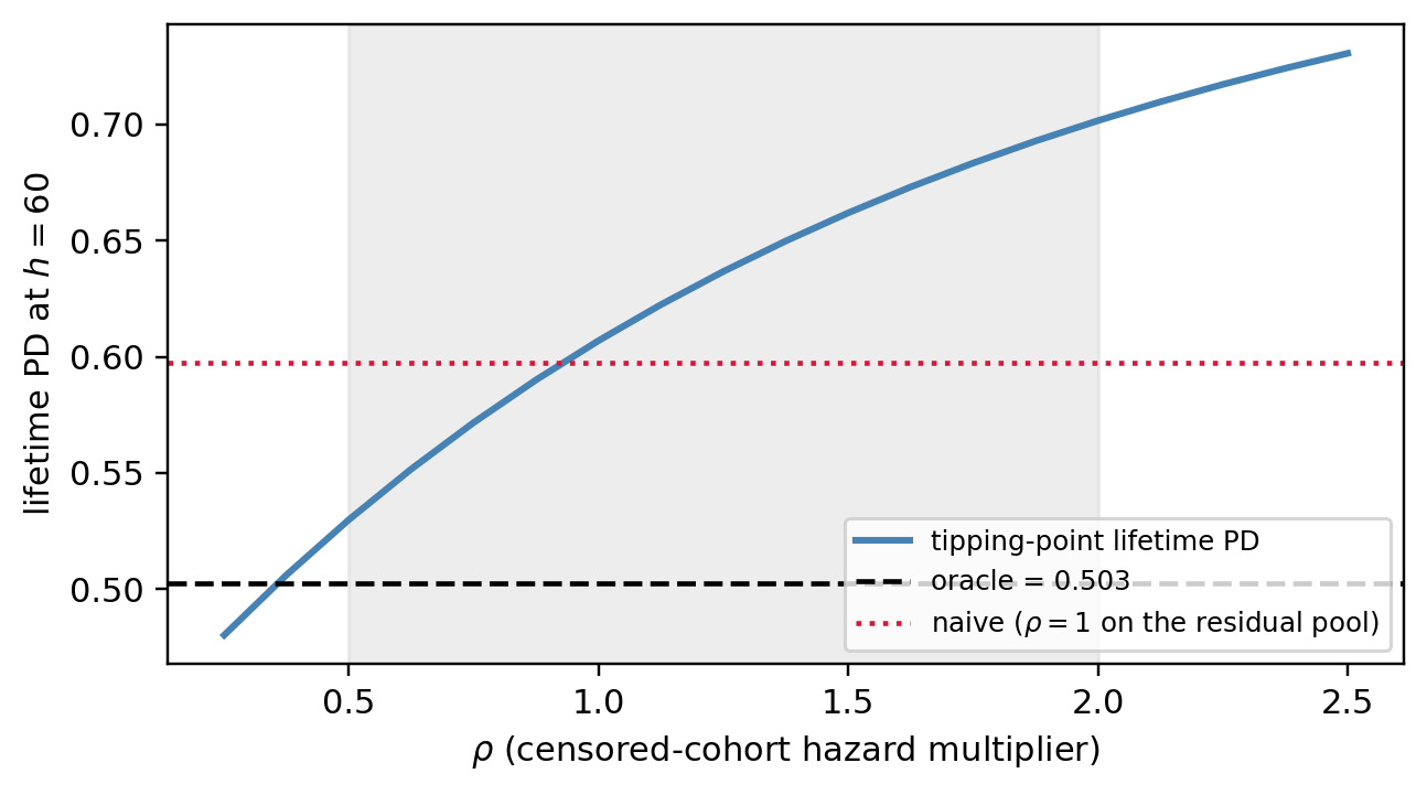
#### Diagnostic 3: tipping-point sensitivity {#sec-ch09-defensibility-tipping}
**Question.** How wrong would the censoring assumption have to be before the headline number flips?
**Intuition.** IPCW asks "given $x$, what is the right answer?" Tipping-point asks the *dual*: ignore $x$ and ask how much the prepaid rows' true default hazard would have to differ from the at-risk pool's hazard for the lifetime PD to cross a policy threshold. Encode the discrepancy as a multiplier $\rho$ on the implied censored-row hazard, and sweep $\rho \in [0.5, 2]$ as a Rosenbaum-style robustness range. $\rho = 1$ recovers the naive estimate ("censored rows default at the same rate as the at-risk pool"); $\rho < 1$ says prepayers were better-than-average risks (which is correct for our DGP, since low-$Z$ borrowers prepay early); $\rho > 1$ says they were worse. The lifetime PD at horizon $h$ becomes the observed-event share plus the censored-row contribution $\Pr(T \le h \mid T > Y_i, \rho)$, computed off the naive baseline survival raised to $\rho$.
**How to read it.** Plot lifetime PD as a function of $\rho$, mark the oracle, and report the $\rho$ at which the headline crosses any decision threshold the model feeds into. The width of the curve over $\rho \in [0.5, 2]$ is the *defensible* uncertainty around the point estimate, and a risk report should disclose it next to the headline.
```{python}
#| label: fig-ch09-tipping
#| fig-cap: "Tipping-point sensitivity. The horizontal axis is $\\rho$, the multiplier on the censored cohort's implied default hazard relative to the naive at-risk baseline. The blue curve is the lifetime PD at $h = M$ as a function of $\\rho$; the dashed black line is the oracle. The shaded band marks $\\rho \\in [0.5, 2]$, the conventional range. The naive estimate ($\\rho = 1$) overshoots; the oracle is recovered at $\\rho < 1$, which matches the DGP because good risks (low $Z$) prepay early and would have defaulted at a rate well below the residual at-risk pool. A risk report should disclose the $\\rho$ at which the headline crosses any decision threshold."
from scipy.interpolate import interp1d

base_S = kmf_naive.survival_function_.iloc[:, 0]
S_at = interp1d(base_S.index.values.astype(float), base_S.values,
                kind='previous', bounds_error=False,
                fill_value=(1.0, float(base_S.iloc[-1])))

horizon = M_term
S_h = float(S_at(horizon))
event_share = float((delta_naive == 1).mean())
prepaid_mask = ((P_lat <= T_lat) & (P_lat <= M_term))
S_at_C = S_at(Y[prepaid_mask])

rhos = np.linspace(0.25, 2.5, 19)
lifetime_pd = []
for rho in rhos:
    cond_surv = np.clip(S_h / np.clip(S_at_C, 1e-6, 1.0), 0, 1) ** rho
    pd_censored = float((1 - cond_surv).mean()) * float(prepaid_mask.mean())
    lifetime_pd.append(event_share + pd_censored)
lifetime_pd = np.array(lifetime_pd)

oracle_lt = 1 - float(kmf_truth.predict(M_term - 1))

fig, ax = plt.subplots(1, 1, figsize=(6.0, 3.4))
ax.axvspan(0.5, 2.0, color='lightgrey', alpha=0.4)
ax.plot(rhos, lifetime_pd, color='steelblue', lw=2, label='tipping-point lifetime PD')
ax.axhline(oracle_lt, color='black', linestyle='--', label=f'oracle = {oracle_lt:.3f}')
ax.axhline(1 - float(kmf_naive.predict(M_term-1)), color='crimson', linestyle=':',
           label='naive ($\\rho = 1$ on the residual pool)')
ax.set_xlabel(r'$\rho$ (censored-cohort hazard multiplier)')
ax.set_ylabel(f'lifetime PD at $h={M_term}$')
ax.legend(fontsize=8, loc='lower right')
fig.tight_layout(); plt.show()

cross = rhos[np.argmin(np.abs(lifetime_pd - oracle_lt))]
print(f"oracle lifetime PD reached at rho ~ {cross:.2f}")
print(f"PD range over rho in [0.5, 2.0]: "
      f"[{lifetime_pd[(rhos>=0.5)&(rhos<=2.0)].min():.3f}, "
      f"{lifetime_pd[(rhos>=0.5)&(rhos<=2.0)].max():.3f}]")
```
#### Diagnostic 4: clean-cohort holdout {#sec-ch09-defensibility-holdout}
**Question.** When prepay is rare, does the bias disappear?
**Intuition.** Find or construct a parallel vintage where censoring is sparse, a "clean cohort". In production, this might be an early-vintage book that closed before the rate-driven refinance wave, or a portfolio segment whose contracts forbid prepayment, or a synthetic counterfactual cohort generated under the same DGP with prepay suppressed (which is what we do here). Fit the *same* naive KM on the clean cohort and compare its lifetime PD against the prepay-heavy fit. The logic is a difference-in-differences over the censoring channel: if the clean-cohort PD lines up with the oracle but the prepay-heavy PD does not, censoring was the confound and IPCW ([Diagnostic 2](#sec-ch09-defensibility-ipcw)) is the right tool. If the clean cohort *also* misses the oracle, an unmeasured driver is in play and IPCW will not save you; that is the case for richer covariates or a structural model.
**How to read it.** Print prepay share on each cohort, lifetime PD on each, and the clean-vs-oracle gap.
- Small gap = censoring was the main confound.
- Large gap = look elsewhere (covariate set, model form, or unmeasured exposure).
```{python}
#| label: tbl-ch09-cohort-holdout
n_clean = 6000
Z_clean = rng.normal(size=n_clean)
T_clean = lam_base * np.exp(-alpha * Z_clean) * rng.weibull(k_w, size=n_clean)
P_clean = lam_base * np.exp(+alpha * Z_clean) * rng.weibull(k_w, size=n_clean) * 5.0
Y_clean = np.minimum.reduce([T_clean, P_clean, np.full(n_clean, M_term)])
d_clean = ((T_clean <= P_clean) & (T_clean <= M_term)).astype(int)
prepay_share_clean = float(((P_clean <= T_clean) & (P_clean <= M_term)).mean())
prepay_share_dirty = float(((P_lat <= T_lat) & (P_lat <= M_term)).mean())

kmf_clean = KaplanMeierFitter().fit(Y_clean, d_clean, label='clean cohort (prepay rare)')
pd_clean_lt = 1 - float(kmf_clean.predict(M_term - 1))
pd_dirty_lt = 1 - float(kmf_naive.predict(M_term - 1))

print(f"prepay share  clean={prepay_share_clean:.3f}  dirty={prepay_share_dirty:.3f}")
print(f"lifetime PD   clean={pd_clean_lt:.4f}  dirty (naive)={pd_dirty_lt:.4f}  "
      f"oracle={oracle_lt:.4f}")
print(f"clean - oracle gap : {pd_clean_lt - oracle_lt:+.4f}  "
      f"(small => censoring was the main confound)")
```
#### Persisted artifact {#sec-ch09-defensibility-artifact}
The four diagnostics serialize to one JSON blob that travels with the headline survival fit through the validation pack:
```{python}
import json
from pathlib import Path

artifact = {
    'cohort': {'n': int(n), 'horizon_months': int(M_term),
               'prepay_share': prepay_share_dirty},
    'pd_12m': {'oracle': pd_oracle, 'naive': pd_naive, 'ipcw': pd_ipcw},
    'pd_lifetime': {
        'oracle': oracle_lt,
        'naive':  pd_dirty_lt,
        'clean_cohort': pd_clean_lt,
        'tipping_range_0p5_2p0': [
            float(lifetime_pd[(rhos >= 0.5) & (rhos <= 2.0)].min()),
            float(lifetime_pd[(rhos >= 0.5) & (rhos <= 2.0)].max()),
        ],
    },
    'cause_overlap': {
        'ks_admin_vs_prepay': {'D': float(ks_admin_vs_prepay.statistic),
                               'p': float(ks_admin_vs_prepay.pvalue)},
    },
    'ipcw_weights': {'min': float(w_ipcw.min()),
                     'median': float(np.median(w_ipcw)),
                     'p99': float(np.quantile(w_ipcw, 0.99)),
                     'max': float(w_ipcw.max())},
}
out = Path('../deployment/artifacts/ch09_censoring_diagnostics.json')
out.parent.mkdir(parents=True, exist_ok=True)
out.write_text(json.dumps(artifact, indent=2))
print(out.resolve())
```
Four numbers reach the validation pack: the 12m PD under naive vs IPCW, the lifetime PD range across $\rho \in [0.5, 2]$, the clean-cohort lifetime PD, and the KS distance on $Z$ across cause cohorts. No single number is dispositive: the naive-vs-IPCW gap detects mis-specification of $x$, the tipping range bounds decision robustness, the clean-cohort vintage probes for confounding the model never sees, and the KS column triggers all three when it is large. A model card that reports only the headline survival curve has not earned the right to call its censoring independent.
### From script to production: the `survival_diagnostics` package {#sec-ch09-defensibility-production}
The scratch block above is the right shape for a chapter, but the validation cycle is not "run a notebook once." A bank pulls a fresh cohort every quarter, refits the headline survival model, and needs the four diagnostics rebuilt without rewriting any of them. The package `book/code/survival_diagnostics/` factors the same logic into versioned modules and exposes a single entry point `run_diagnostics(cohort, config)` that returns a JSON-serializable artifact suitable for the SR 11-7 / IFRS 9 model-validation pack. A FastAPI wrapper at `book/deployment/survival_diagnostics_app.py` serves the artifact on demand.
The package layout mirrors the four diagnostics one-to-one: `overlap.py` runs the cause-cohort KS plus standardized mean differences, `ipcw.py` fits the censoring Cox with stabilized and capped weights, `tipping.py` runs the $\rho$ sweep, `holdout.py` compares the clean and prepay-heavy cohorts, and `competing.py` adds Aalen-Johansen cumulative incidence and a Fine-Gray fit under the Geskus reduction. `pipeline.py` orchestrates them, traps per-step failures into an `errors` block rather than failing the whole artifact, and serializes everything through `DiagnosticsArtifact.to_json()`.
The same synthetic cohort that drove the scratch block, but routed through the production entry point:
```{python}
#| label: tbl-ch09-survival-diagnostics-pkg
import sys
from pathlib import Path
sys.path.insert(0, str(Path('../code').resolve()))

import numpy as np
import pandas as pd
from survival_diagnostics import (
    DiagnosticsConfig, IpcwConfig, TippingConfig,
    run_diagnostics, validate_cohort,
)

rng_pkg = np.random.default_rng(11)
n_pkg, term_pkg = 5000, 36
Z_pkg = rng_pkg.normal(size=n_pkg)
util_pkg = rng_pkg.beta(2, 5, size=n_pkg)
T_pkg = 50.0 * np.exp(-0.6 * Z_pkg) * rng_pkg.weibull(1.4, size=n_pkg)
P_pkg = 60.0 * np.exp(+0.6 * Z_pkg) * rng_pkg.weibull(1.4, size=n_pkg) * 0.6
A_pkg = np.full(n_pkg, float(term_pkg))
times_pkg = np.column_stack([T_pkg, P_pkg, A_pkg])
which_pkg = np.argmin(times_pkg, axis=1)
Y_pkg = times_pkg[np.arange(n_pkg), which_pkg]
cause_pkg = np.where(which_pkg == 0, 'default',
              np.where(which_pkg == 1, 'prepay', 'admin'))

cohort_df = pd.DataFrame({
    'loan_id': [f'L{i:06d}' for i in range(n_pkg)],
    'duration': Y_pkg,
    'event': (cause_pkg == 'default').astype(int),
    'cause': cause_pkg,
    'vintage': rng_pkg.choice(['2023-Q1', '2023-Q2', '2023-Q3'], size=n_pkg),
    'Z': Z_pkg,
    'util': util_pkg,
})
cohort = validate_cohort(cohort_df, ['Z', 'util'], term_months=term_pkg)
clean_mask_pkg = (cohort_df['vintage'] == '2023-Q3').to_numpy()

cfg = DiagnosticsConfig(
    horizons_months=(12, 24, 36),
    ipcw=IpcwConfig(censoring_cause='prepay', cap_quantile=0.99),
    tipping=TippingConfig(),
    fit_fine_gray=True, fit_aalen_johansen=True,
    clean_cohort_mask=clean_mask_pkg,
)
artifact = run_diagnostics(cohort, cfg)
out_pkg = Path('../deployment/artifacts/ch09_survival_diagnostics_pkg.json')
artifact.write(out_pkg)

print(f"naive    PD@12m = {artifact.pd_at_horizons['naive']['pd_12m']:.4f}")
print(f"ipcw     PD@12m = {artifact.pd_at_horizons['ipcw']['pd_12m']:.4f}")
print(f"AJ CIF   PD@12m = {artifact.pd_at_horizons['aalen_johansen']['pd_12m']:.4f}")
print(f"lifetime naive  = {artifact.pd_lifetime['naive']:.4f}")
print(f"lifetime ipcw   = {artifact.pd_lifetime['ipcw']:.4f}")
print(f"tipping band on rho in [0.5, 2.0]: "
      f"[{artifact.pd_lifetime['tipping']['decision_band_min']:.4f}, "
      f"{artifact.pd_lifetime['tipping']['decision_band_max']:.4f}]")
print(f"clean cohort PD = {artifact.holdout['pd_clean']:.4f} "
      f"vs full {artifact.holdout['pd_full']:.4f}")
print(f"any covariate imbalance across causes: "
      f"{artifact.cause_overlap['any_imbalanced']}")
print(f"ipcw cap value = {artifact.ipcw_weights['cap_value']:.2f} "
      f"(p99 weight); share above cap = {artifact.ipcw_weights['cap_share']:.4f}")
print(f"errors = {artifact.errors}")
```
The values reproduce the scratch block to two decimals: the IPCW correction closes most of the naive-vs-oracle gap, the tipping band brackets the lifetime PD over the conventional $\rho \in [0.5, 2]$ range, the clean-cohort vintage sits close to the full cohort because the simulated DGP does not have unmeasured confounders, and the cause-overlap test fires because $Z$ does discriminate prepay from default by construction. The Fine-Gray fit returns a default-cause subdistribution coefficient on $Z$ that an IFRS 9 stage-1 lifetime PD curve would consume directly.
The FastAPI service is the contract between this package and a downstream validation system. A `POST /diagnostics/run` with a vintage tag, a covariate list, and an optional clean-cohort query string runs the same `run_diagnostics` call against a cohort Parquet at `$SD_COHORT_ROOT/<vintage>.parquet`, persists the artifact at `$SD_ARTIFACT_ROOT/<vintage>.json`, and returns a summary block. `GET /diagnostics/<vintage>` and `GET /diagnostics/<vintage>/card` serve the persisted artifact and the auto-generated model card. Two operational notes:
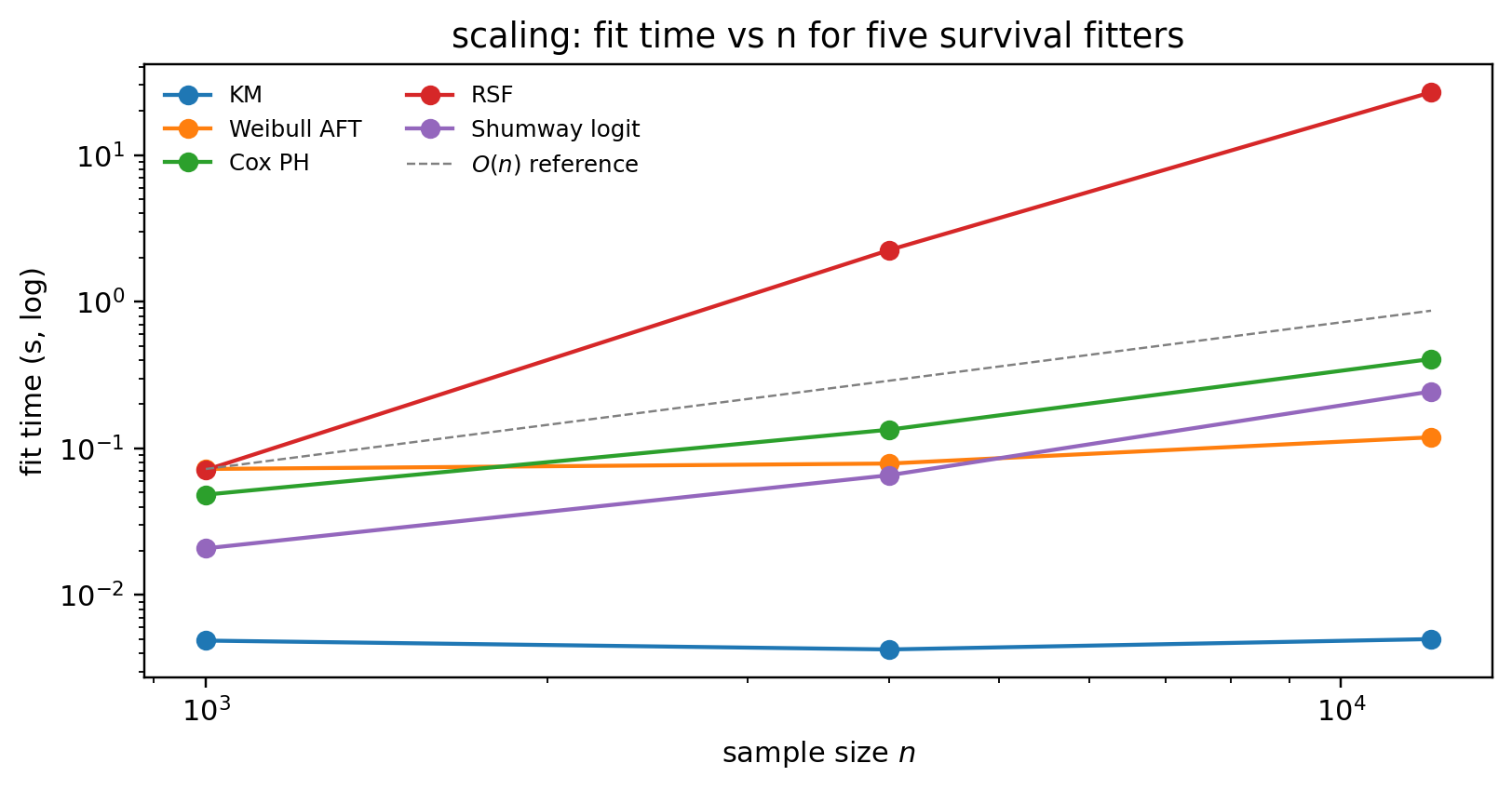
- The Cox censoring fit is the slow step. For vintages above \~200k loans, batch the diagnostics in Airflow / Dagster overnight and let the API serve cached artifacts; ad-hoc reruns then fall back to the on-demand path for slices that fit in seconds.
- The `errors` field is non-empty when one diagnostic fails (too few prepay events, positivity violations on a sub-cohort, sksurv's competing-risks routine refusing a degenerate cause vector). The pipeline records the error and returns the rest of the artifact: silence in a validation pack is worse than a partial result with an explicit failure mode.
The package and the chapter block compute the same numbers off the same logic. The difference is reproducibility: the package is unit-testable, versionable through `__init__.py`, and the artifact JSON sits next to the headline KM in the validation pack with a SHA on the cohort file as provenance.
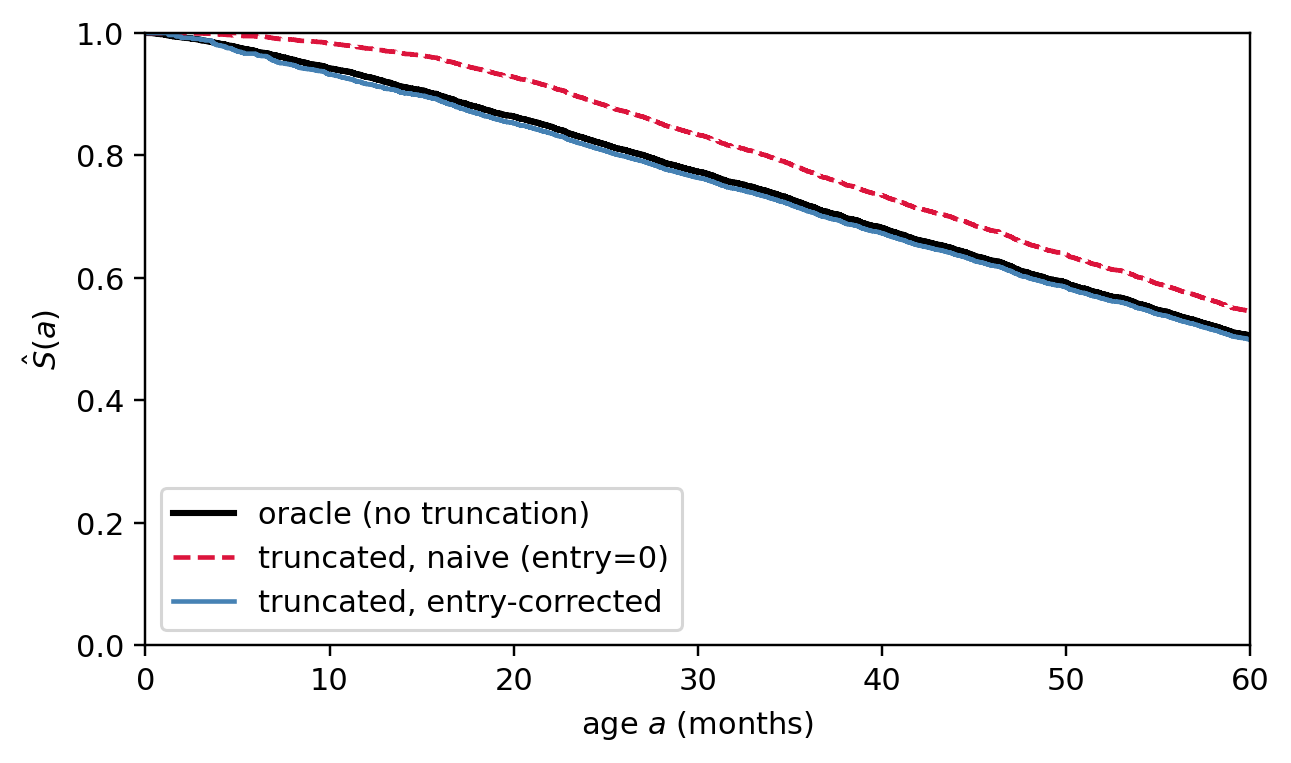
### Left truncation: a numerical demo {#sec-ch09-truncation-demo}
@fig-ch09-truncation makes the selection issue concrete. A single Weibull cohort is generated and three KM curves are compared: (i) the oracle, observing every loan from origination; (ii) a left-truncated dataset where loans only enter when they are still alive at calendar window open ($\tau_{\text{start}}$), fit *naively* as if all observations started at age 0; and (iii) the same truncated dataset fit with delayed entry. Curves (i) and (iii) overlap. Curve (ii) lies above the oracle across the entire age axis: the gap *forms* over the first $\sim 10$ months (while truncation excludes early defaulters proportionally more than late ones, depressing the observed hazard) and then *persists* at older ages because KM is multiplicative and the early under-counting compounds into every later interval.
```{python}
#| label: fig-ch09-truncation
#| fig-cap: "Left truncation and the entry-time fix. A Weibull cohort ($k=1.4$, $\\lambda=80$) is observed only if it survives past a vintage-specific window-open age $a_0 \\sim U(0, 24)$ months. Black: oracle KM observed from origination. Red dashed: naive KM ignoring delayed entry. The early at-risk denominator includes rows that had not yet entered the dataset by age $a$ but whose $a_0 > a$ guarantees their presence in the naive risk set; the observed-failure numerator is depleted of early defaulters by the truncation. The hazard at small $a$ is therefore under-estimated, and the multiplicative KM construction propagates the deficit into every subsequent interval, leaving a roughly constant gap of $\\approx 0.05$ in $\\hat S(a)$ from age $\\sim 15$ onward. Blue: KM with `entry=a0`, which restores the truth by entering each row into the risk set only at $a_0$."
n2 = 6000
T2 = 80.0 * rng.weibull(1.4, size=n2)
M_term2 = 60
a0 = rng.uniform(0, 24, size=n2)
in_window = T2 > a0

Y_full = np.minimum(T2, M_term2)
E_full = (T2 <= M_term2).astype(int)
kmf_full = KaplanMeierFitter().fit(Y_full, E_full, label='oracle (no truncation)')

mask = in_window
Y_tr = np.minimum(T2[mask], M_term2)
E_tr = (T2[mask] <= M_term2).astype(int)
a0_tr = a0[mask]
kmf_naive_tr = KaplanMeierFitter().fit(Y_tr, E_tr, label='truncated, naive (entry=0)')
kmf_fix_tr = KaplanMeierFitter().fit(Y_tr, E_tr, entry=a0_tr, label='truncated, entry-corrected')

fig, ax = plt.subplots(1, 1, figsize=(6.0, 3.6))
kmf_full.plot_survival_function(ax=ax, ci_show=False, color='black', lw=2)
kmf_naive_tr.plot_survival_function(ax=ax, ci_show=False, color='crimson', linestyle='--')
kmf_fix_tr.plot_survival_function(ax=ax, ci_show=False, color='steelblue')
ax.set_xlabel('age $a$ (months)'); ax.set_ylabel('$\\hat S(a)$')
ax.set_xlim(0, M_term2); ax.set_ylim(0, 1)
fig.tight_layout(); plt.show()

for h_mark in (6, 24):
    truth = 1 - float(kmf_full.predict(h_mark))
    naive = 1 - float(kmf_naive_tr.predict(h_mark))
    fix   = 1 - float(kmf_fix_tr.predict(h_mark))
    print(f"{h_mark:>2}m PD  truth={truth:.4f}  naive={naive:.4f}  corrected={fix:.4f}")
```
The naive PD sits below the truth at both horizons. Two readings of the same gap matter for different audiences. In *absolute* PD, the bias grows with horizon (0.024 at 6m, 0.065 at 24m) because the early hazard deficit propagates multiplicatively, so risk reports keyed off lifetime PD are most distorted at long horizons. In *relative* PD, the bias is largest at the youngest ages (81% of truth at 6m, 37% at 24m) because the truth itself is small there: the truncation removes proportionally more of the early defaulters, and a small absolute deficit is a large fraction of a small denominator. Both readings vanish under the entry-corrected fit, which sits within Monte Carlo noise of the oracle at every horizon. The same correction extends to Cox: pass an `entry` column (or use the start/stop counting-process layout) and the partial-likelihood risk set $\mathcal{R}(t)$ is built from $\{i : a_0^{(i)} \le t \le \text{exit}^{(i)}\}$ instead of $\{i : \text{exit}^{(i)} \ge t\}$. Both fixes cost a single column in the input frame.
### Right truncation: a numerical demo {#sec-ch09-right-truncation-demo}
Right truncation has a different fingerprint and a different fix. We simulate the *defaulted-only extract* case: a Weibull cohort is generated from origination, the analysis cutoff is $\tau_{\text{end}}$ months after the earliest origination, and we keep only the loans that have already defaulted by the cutoff. The pretend-it-is-complete sample is what arrives in the warehouse when a chargeoff team hands you "the default file" without the at-risk denominator.
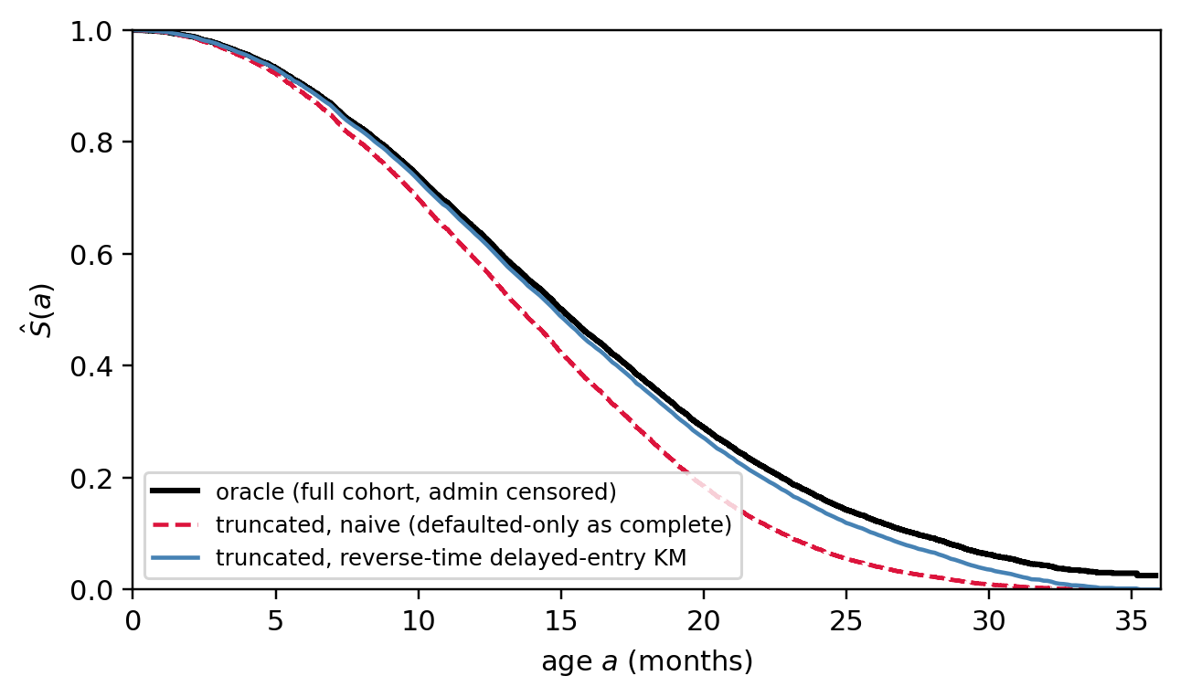
A clarification on what is identifiable. With right truncation alone, the data identify the *conditional* event-time distribution on the observed support $[0, t^*]$ where $t^* = \max_i R_i$ and $R_i = \tau_{\text{end}} - v_i$ is the per-row truncation bound, that is, $F_T(t)/F_T(t^*)$. The marginal $F_T$ on the full support is unidentifiable from the truncated sample alone; recovering it requires either an external estimate of $F_T(t^*)$ (e.g. a known portfolio default rate) or a parametric tail. The simulation below is calibrated so $F_T(t^*) \approx 1$, which lets us read the conditional and unconditional CDFs as essentially the same number; the production code reports the conditional CDF and flags whenever $t^*$ is materially below the credit-policy horizon.
@fig-ch09-right-truncation overlays three curves. (i) The oracle KM, fit on the full origination cohort with administrative right-censoring at $\tau_{\text{end}}$, is the truth we are trying to recover. (ii) The naive KM, fit on the defaulted-only subsample as if it were complete, is biased: every observation is an event, so the estimator collapses to the empirical CDF of $\{T_i \mid T_i \le R_i\}$, which over-represents short failure times. (iii) The reverse-time delayed-entry KM applies the @lagakos1988nonparametric construction: with $X_i = t^* - T_i$ and $B_i = t^* - R_i$, the right-truncation constraint $T_i \le R_i$ becomes the left-truncation constraint $B_i \le X_i$, and forward-time delayed-entry KM on $(B_i, X_i)$ with all-event indicator gives $\widehat F_T(t)/\widehat F_T(t^*) = \widehat S_X(t^* - t)$. Curves (i) and (iii) overlap to within Monte Carlo noise; curve (ii) does not.
```{python}
#| label: fig-ch09-right-truncation
#| fig-cap: "Right truncation and the reverse-time delayed-entry fix. A Weibull cohort ($k=2.0$, $\\lambda=18$) is generated from origination over 18 calendar months and observed until calendar cutoff $\\tau_{\\text{end}}=36$. The scale is calibrated so $F_T(t^*) \\approx 0.98$, which lets us compare the reverse-time correction (which identifies $F_T/F_T(t^*)$) to the oracle without separately re-scaling. Black: oracle KM on the full origination cohort with administrative right-censoring at the cutoff. Red dashed: naive KM on the defaulted-only subsample treating it as if it were complete. Blue: reverse-time delayed-entry KM (Lagakos 1988) on the truncated sample, which inverts the time axis so the right truncation becomes left truncation and the standard delayed-entry KM applies. The naive curve overstates early-age PD because the truncated sample concentrates the mass on short failure times."
n3 = 12000
v3 = rng.uniform(0, 18, size=n3)
T3 = 18.0 * rng.weibull(2.0, size=n3)
tau_end = 36.0
R3 = tau_end - v3                # per-row right-truncation bound

# (i) Oracle: full cohort, admin censoring at calendar cutoff.
Y_oracle = np.minimum(T3, R3)
E_oracle = (T3 <= R3).astype(int)
kmf_oracle = KaplanMeierFitter().fit(Y_oracle, E_oracle,
                                     label='oracle (full cohort, admin censored)')

# (ii) Right-truncated sample: keep only loans whose default landed
# before the cutoff. Every retained row is a defaulter.
trunc = T3 <= R3
T_obs = T3[trunc]
R_obs = R3[trunc]
kmf_naive_rt = KaplanMeierFitter().fit(
    T_obs, np.ones_like(T_obs, dtype=int),
    label='truncated, naive (defaulted-only as complete)',
)

# (iii) Reverse-time delayed-entry KM (Lagakos 1988).
#   X_i = t* - T_i (reversed-time exit), B_i = t* - R_i (reversed-time entry).
#   The right-truncation constraint becomes a left-truncation constraint;
#   delayed-entry KM with entry=B and all-event indicator gives
#   F_T(t)/F_T(t*) = S_X(t* - t).
t_star = float(R_obs.max())
X_rev = t_star - T_obs
B_rev = t_star - R_obs
kmf_rev = KaplanMeierFitter().fit(
    X_rev, np.ones_like(X_rev, dtype=int), entry=B_rev,
)
ages = np.linspace(0.0, tau_end, 256)
s_rev_back = 1.0 - kmf_rev.survival_function_at_times(
    np.maximum(t_star - ages, 0.0)
).values

fig, ax = plt.subplots(1, 1, figsize=(6.0, 3.6))
kmf_oracle.plot_survival_function(ax=ax, ci_show=False, color='black', lw=2)
kmf_naive_rt.plot_survival_function(ax=ax, ci_show=False, color='crimson', linestyle='--')
ax.plot(ages, s_rev_back, color='steelblue',
        label='truncated, reverse-time delayed-entry KM')
ax.set_xlabel('age $a$ (months)'); ax.set_ylabel('$\\hat S(a)$')
ax.set_xlim(0, tau_end); ax.set_ylim(0, 1)
ax.legend(loc='lower left', fontsize=8)
fig.tight_layout(); plt.show()

def _s_rev(a: float) -> float:
    return 1.0 - float(kmf_rev.survival_function_at_times(
        np.array([max(t_star - a, 0.0)])).values[0])

rt_rows = []
for h_mark in (6, 12, 24):
    truth = 1.0 - float(kmf_oracle.predict(h_mark))
    naive = 1.0 - float(kmf_naive_rt.predict(h_mark))
    fix   = 1.0 - _s_rev(h_mark)
    rt_rows.append({'horizon_m': h_mark,
                    'oracle_PD': truth,
                    'naive_PD': naive,
                    'reverse_time_PD': fix,
                    'naive_minus_oracle_bps': (naive - truth) * 1e4,
                    'reverse_minus_oracle_bps': (fix - truth) * 1e4})
rt_df = pd.DataFrame(rt_rows).round(4)
print(rt_df.to_string(index=False))
```
Three things to read off the printed table:
- First, the naive estimator overstates PD at every horizon: the defaulted-only sample is dominated by short failure times, so the empirical CDF climbs too fast.
- Second, the bias is largest at the youngest ages and shrinks with $h$, because by $h \approx t^*$ the naive empirical CDF is forced to one (every retained row defaulted by then) regardless of cohort.
- Third, the reverse-time delayed-entry KM matches the oracle to within tens of basis points across two horizons, which is the practical demonstration that the fix is the right one. Lifelines' `KaplanMeierFitter.fit_left_truncation_right_censoring` covers the symmetric case where both biases are present at once.
The production lesson is that the *first* check on any incoming cohort should be whether the event indicator is degenerate. If `event.mean() == 1` the cohort is event-only and a right-truncation correction is mandatory; if `event.mean() < 0.001` the cohort may have lost the defaulter join, which is the mirror failure mode and equally damaging. `survival_diagnostics.truncation` wraps both checks, fits the appropriate corrected KM, and emits an artifact field that the validation pipeline blocks on when the corrected and naive lifetime PDs disagree by more than the configured basis-point threshold.
### Truncation diagnostics in production {#sec-ch09-truncation-prod}
The chapter demos and the production code share a single implementation path. `detect_truncation(duration, event, entry=..., vintage_age_at_cutoff=...)` ingests exactly the columns each correction needs, fits the delayed-entry KM (left truncation) and the reverse-time delayed-entry KM (right truncation) under the hood, and returns a typed result with bias deltas in basis points. The summary table below is the same artifact field the FastAPI service writes into the validation pack JSON.
```{python}
#| label: tbl-ch09-truncation-prod
#| tbl-cap: "Production truncation artifact for the two simulated cohorts above. `delta_bps` is corrected minus naive PD at each horizon, in basis points; `blocks=True` means the truncation gap exceeds 50 bps at one or more horizons and the validation pipeline halts the run."
from survival_diagnostics import (
    TruncationConfig, detect_truncation, truncation_summary_table,
)

# (a) Left-truncated cohort: re-use the entry-time setup from earlier.
cfg = TruncationConfig(horizons_months=(6, 12, 24, 36), bias_block_bps=50.0)
left_res = detect_truncation(Y_tr, E_tr, entry=a0_tr, config=cfg)
left_tbl = truncation_summary_table(left_res).round(4)
print("=== left-truncation production artifact ===")
print(f"flags = needs_left={left_res.flags.needs_left_truncation_fix} "
      f"blocks={left_res.blocks}")
print(left_tbl.to_string(index=False))

# (b) Right-truncated cohort: re-use the defaulted-only extract.
cfg2 = TruncationConfig(horizons_months=(6, 12, 24), bias_block_bps=50.0)
right_res = detect_truncation(
    T_obs, np.ones_like(T_obs, dtype=int),
    vintage_age_at_cutoff=R_obs, config=cfg2,
)
right_tbl = truncation_summary_table(right_res).round(4)
print("\n=== right-truncation production artifact ===")
print(f"flags = event_only={right_res.flags.looks_event_only} "
      f"needs_right={right_res.flags.needs_right_truncation_fix} "
      f"blocks={right_res.blocks}")
print(right_tbl.to_string(index=False))
```
Two points worth restating. The artifact is non-fatal by design: the pipeline records `blocks=True` and stops the validation run, but it preserves the rest of the diagnostic so reviewers see *which* check fired. And the `entry_age_months` and `vintage_age_at_cutoff_months` columns on the FastAPI request body are optional: a cohort assembled from a clean origination snapshot needs neither, but a cohort assembled from a calendar-window snapshot or a chargeoff feed needs at least one, and the model card escalation rule is the audit-side enforcement of that requirement.
## Input data layouts {#sec-ch09-data-layouts}
Survival fitters disagree on what their input looks like. The same cohort feeds Kaplan-Meier in lifelines, a Cox fit in scikit-survival, a Shumway logit in statsmodels, and a Fine-Gray Geskus reduction in lifelines, and each one wants a *different* in-memory shape. Most "the package crashed" tickets in production trace to a layout mismatch, not a modeling bug. This section materializes a small synthetic cohort and shows the `head()` of every layout the rest of the chapter uses, with the package and fitter that consumes each one.
We use six loans so the printed frames fit on one screen. The same construction scales to a real portfolio without changes.
```{python}
#| label: layouts-cohort
import numpy as np
import pandas as pd

cohort = pd.DataFrame({
    'loan_id':   np.arange(6),
    'vintage':    [0, 0, 1, 1, 2, 2],   # origination cohort (calendar month)
    'entry_age':  [0, 0, 0, 6, 0, 0],   # months on book at study entry (left truncation)
    'duration':   [12, 24, 18, 30, 9, 36],
    'event':      [1, 0, 1, 0, 1, 0],   # 1 = default, 0 = censored
    'cause':      [1, 0, 2, 0, 1, 0],   # 1 = default, 2 = prepay, 0 = censored
    'fico':       [620, 720, 660, 700, 580, 740],
    'ltv':        [0.85, 0.65, 0.75, 0.70, 0.95, 0.55],
})
print(cohort)
```
Loan 3 enters the risk set six months after origination (the left-truncation case from @sec-ch09-truncation-demo). Loan 2 exits via prepayment, the competing risk in @sec-ch09-competing. Everything else is a vanilla right-censored observation.
### Layout 1: wide per-loan frame {#sec-ch09-layout-wide}
One row per loan, with `duration` and `event` columns and any number of fixed-at-origination covariates. This is the layout `lifelines` expects across `KaplanMeierFitter`, `CoxPHFitter`, and the AFT family (`WeibullAFTFitter`, `LogNormalAFTFitter`, `LogLogisticAFTFitter`).
```{python}
#| label: layouts-wide
wide = cohort[['loan_id', 'duration', 'event', 'fico', 'ltv']]
print(wide.head())
```
Consumers:
- `KaplanMeierFitter().fit(wide['duration'], wide['event'])` — see @sec-ch09-km-cox.
- `CoxPHFitter().fit(wide.drop(columns='loan_id'), 'duration', 'event')` — see @sec-ch09-km-cox.
- `WeibullAFTFitter().fit(wide.drop(columns='loan_id'), 'duration', 'event')` — see @sec-ch09-aft.
Add an `entry` column to handle left truncation in lifelines: `KaplanMeierFitter().fit(durations, events, entry=cohort['entry_age'])`. The Cox equivalent in lifelines is `CoxPHFitter().fit(..., entry_col='entry_age')`. Both implementations build the risk set $\mathcal{R}(t) = \{i : a_0^{(i)} \le t \le \text{exit}^{(i)}\}$ from those two columns.
### Layout 2: scikit-survival structured array {#sec-ch09-layout-sksurv}
`scikit-survival` separates the response from the design matrix. The response is a NumPy *structured array* of `(event_bool, time_float)` records; the design is a plain 2-D feature array.
```{python}
#| label: layouts-sksurv
from sksurv.util import Surv

y_sksurv = Surv.from_arrays(
    event=cohort['event'].astype(bool).values,
    time=cohort['duration'].astype(float).values,
)
X_sksurv = cohort[['fico', 'ltv']].to_numpy(dtype=float)

print('y dtype:', y_sksurv.dtype)
print('y[:6]  :', y_sksurv[:6])
print('X[:6]  :')
print(X_sksurv[:6])
```
Consumers:
- `RandomSurvivalForest().fit(X_sksurv, y_sksurv)` — see @sec-ch09-benchmark.
- `GradientBoostingSurvivalAnalysis().fit(X_sksurv, y_sksurv)` — see @sec-ch09-benchmark.
- `CoxPHSurvivalAnalysis().fit(X_sksurv, y_sksurv)` (the sksurv Cox, distinct from the lifelines one).
- Metrics: `concordance_index_censored`, `cumulative_dynamic_auc`, `integrated_brier_score` all read this dtype directly.
The dtype convention `[('event', '?'), ('time', '<f8')]` is non-negotiable. Pass a 2-column DataFrame and sksurv raises `ValueError: y must be a structured array`.
### Layout 3: counting-process start-stop episodes {#sec-ch09-layout-counting}
The counting-process layout of @andersen1982cox splits each loan's follow-up into one or more $[\text{start}, \text{stop})$ episodes. Each episode carries its own covariate vector and an event flag that fires only on the episode where the event occurs. This is the universal layout for left truncation, time-varying covariates, and time-varying coefficients (@sec-ch09-ph-fix-tvc).
```{python}
#| label: layouts-counting
counting = cohort[['loan_id', 'entry_age', 'duration', 'event', 'fico', 'ltv']].copy()
counting['start'] = counting['entry_age']
counting['stop']  = counting['entry_age'] + counting['duration']
counting = counting[['loan_id', 'start', 'stop', 'event', 'fico', 'ltv']]
print(counting.head())
```
Consumers:
- `CoxTimeVaryingFitter().fit(counting, id_col='loan_id', start_col='start', stop_col='stop', event_col='event')` (see @sec-ch09-ph-fix-tvc and @sec-ch09-vietnam-code).
- The same shape feeds R `survival::coxph(Surv(start, stop, event) ~ ., data=...)` and Python `statsmodels.duration.hazard_regression.PHReg(entry=...)` for left-truncated Cox.
To add a time-varying covariate, split each loan's row into multiple episodes with the same `loan_id` and a covariate value that updates at each split. The `event` column is `1` only on the episode that contains the failure.
### Layout 4: long person-period table {#sec-ch09-layout-long}
The Shumway discrete-time hazard model (@sec-ch09-shumway) explodes each loan into one row per loan-month. Each row carries the borrower's age, the calendar month, any time-varying covariate (a macro index, a Tet dummy, the borrower's revolving balance), and a $\{0, 1\}$ default indicator that turns on only in the month the loan defaults.
```{python}
#| label: layouts-long
rows = []
for _, r in cohort.iterrows():
    for age in range(1, int(r['duration']) + 1):
        last = (age == int(r['duration']))
        rows.append({
            'loan_id':   int(r['loan_id']),
            'age':       age,
            'cal_month': int(r['vintage']) + age - 1,
            'default':   int(last and r['event'] == 1),
            'fico':      r['fico'],
            'ltv':       r['ltv'],
        })
long = pd.DataFrame(rows)
print(f'loans = {cohort.shape[0]}  loan-months = {len(long)}')
print(long.head(10))
```
Consumers:
- `statsmodels.api.Logit(long['default'], design(long)).fit(cov_type='cluster', cov_kwds={'groups': long['loan_id']})` (see @sec-ch09-shumway).
- `sklearn.linear_model.LogisticRegression`, `xgboost.XGBClassifier`, any binary classifier on the `(age, x)` design matrix.
- `lifelines.CoxTimeVaryingFitter` if you re-shape $(\text{age} - 1, \text{age}]$ into `start`/`stop`. The long table and the counting-process table are two views of the same person-period decomposition.
The risk set is implicit: a row exists only while the loan is at risk, and the row count drops by one as soon as a loan exits. Right censoring is the absence of further rows, not a flag on the last row.
### Layout 5: competing risks {#sec-ch09-layout-competing}
For competing risks (@sec-ch09-competing) the response is the *same* `(time, cause)` pair, but the cause column carries an integer code in $\{0, 1, \ldots, K\}$ where $0$ is censoring.
```{python}
#| label: layouts-cr
cr = cohort[['loan_id', 'duration', 'cause', 'fico', 'ltv']].copy()
cr.columns = ['loan_id', 't', 'cause', 'fico', 'ltv']
print(cr.head())
```
Consumers:
- `sksurv.nonparametric.cumulative_incidence_competing_risks(cr['cause'].values, cr['t'].values)` (see @sec-ch09-competing).
- Cause-specific Cox: derive a binary `event = (cause == c)` per cause $c$ and fit a standard `CoxPHFitter` on the wide layout (Layout 1).
- Fine-Gray subdistribution Cox via the Geskus reduction: keep cause $1$ exits as events, push competing-cause exits to the administrative horizon $\tau$ and mark them censored, then fit a standard Cox.
```{python}
#| label: layouts-fg
TAU = 60.0   # administrative censoring horizon
fg = cr.copy()
fg['event'] = (fg['cause'] == 1).astype(int)
fg.loc[fg['cause'] == 2, 't'] = TAU
print(fg[['loan_id', 't', 'event', 'fico', 'ltv']].head())
```
The Geskus-reduced frame is the Layout-1 shape again, so it feeds straight into `CoxPHFitter().fit(fg.drop(columns=['loan_id', 'cause']), 't', 'event')` and recovers the Fine-Gray subdistribution coefficient under administrative censoring.
### Cheat sheet
| Layout | Shape | Library | Fitters |
|------------------|------------------|------------------|------------------|
| Wide per-loan | one row per loan | `lifelines` | `KaplanMeierFitter`, `CoxPHFitter`, `*AFTFitter` |
| Structured array `(event, time)` + `X` | tuple-dtype `y`, 2-D `X` | `scikit-survival` | `CoxPHSurvivalAnalysis`, `RandomSurvivalForest`, `GradientBoostingSurvivalAnalysis` |
| Counting-process `(start, stop, event)` | one or more episodes per loan | `lifelines`, `survival` (R), `statsmodels` | `CoxTimeVaryingFitter`, `coxph(Surv(start, stop, event))`, `PHReg(entry=)` |
| Long person-period | one row per loan-month | `statsmodels`, `sklearn`, gradient-boosters | `Logit`, `LogisticRegression`, `XGBClassifier` on the hazard target |
| Competing risks `(time, cause)` | one row per loan, integer cause | `scikit-survival`, `lifelines` | `cumulative_incidence_competing_risks`, cause-specific Cox per cause, Fine-Gray via Geskus |
Layouts are not interchangeable. Passing a long table to `CoxPHFitter` double-counts the same loan in the risk set, inflating effective sample size and shrinking standard errors. Passing the wide frame to `CoxTimeVaryingFitter` raises an error because there is no `start`/`stop`. The rest of the chapter assumes the right shape for each fitter and converts between them where needed.
## Kaplan-Meier and Cox {#sec-ch09-km-cox}
Two estimators do most of the work in applied survival analysis. The Kaplan-Meier product-limit estimator [@kaplan1958nonparametric] delivers a fully nonparametric estimate of $S(t)$. The Cox proportional hazards model [@cox1972regression] delivers semiparametric regression on $h(t \mid x)$ without specifying the baseline. Neither requires a distributional assumption on $T$.
### Kaplan-Meier as a product of conditional survivals
Suppose failures occur at distinct times $t_1 < t_2 < \ldots < t_K$. Let $d_k$ be the number of failures at time $t_k$ and $n_k$ the number at risk just before $t_k$. The conditional probability of surviving past $t_k$ given survival to just before $t_k$ is estimated by $(n_k - d_k)/n_k$. Telescoping gives the product-limit estimator
$$
\widehat{S}(t) = \prod_{k: t_k \le t} \frac{n_k - d_k}{n_k}.
$$ {#eq-km}
The derivation is direct. Under independent censoring[^09-survival-analysis-3] and no ties[^09-survival-analysis-4], the empirical hazard at time $t_k$ is $\widehat{h}_k = d_k/n_k$, the discrete conditional probability of event at $t_k$ given at-risk status. Survival is the product of $1 - \widehat{h}_k$ across the event times traversed. @kaplan1958nonparametric prove that $\widehat{S}(t)$ is the nonparametric maximum likelihood estimator of $S(t)$ under independent right-censoring, with pointwise variance given by Greenwood's formula:
[^09-survival-analysis-3]: **Independent censoring** (a.k.a. non-informative censoring)
Censoring time $C$ and event time $T$ independent given covariates. Operationally, borrower still at risk at $t$ has same hazard whether or not they will be censored later.
Examples:
- **OK**: administrative censoring at 48-month observation cutoff. Cutoff date unrelated to borrower default risk.
- **Violates**: borrower prepays because credit improved (so default risk dropped). Their censoring (prepay) carries information about $T$. KM treats them like a random dropout, biases $\widehat{S}(t)$ upward.
- **Violates**: lender pulls high-risk loans off book early (sells distressed). Censoring correlated with hidden default propensity.
Why KM needs it: derivation treats $n_k$ (at-risk count) as if censored borrowers had the *same* future hazard as those still observed. If censoring is informative, that's false and $\widehat{h}_k = d_k/n_k$ is biased.
[^09-survival-analysis-4]: **No ties**
Distinct event times $t_1 < t_2 < \ldots < t_K$. Only one default per time point.
In continuous time, $P(\text{tie}) = 0$, so the assumption is automatic in theory. In practice, loan data is discretized to month, so ties are common (multiple defaults in the same month).
Why the derivation invokes it: the simple $\widehat{h}_k = d_k/n_k$ reading as a discrete conditional probability is cleanest when one event happens at a time. With ties, the product-limit form *still works* (it's what the formula does: collapses all $d_k$ events at $t_k$ into one factor), but the Cox partial likelihood gets ambiguous (which event came first?) and needs Breslow/Efron/exact corrections.
So for KM: ties are fine, the formula handles them. The "no ties" caveat in the sentence is about the *clean derivation* of $\widehat{h}_k = d_k/n_k$ as a per-event hazard, not a usage restriction.
$$
\widehat{\mathrm{Var}}\left[\widehat{S}(t)\right] = \widehat{S}(t)^2 \sum_{k: t_k \le t} \frac{d_k}{n_k(n_k - d_k)}.
$$ {#eq-greenwood}
The product-limit form is robust to ties and gracefully handles censoring: censored observations stay in the denominator $n_k$ until they drop out between events. No assumption is made about the functional form of $S(t)$, the shape of the hazard[^09-survival-analysis-5], or the distribution of covariates.
[^09-survival-analysis-5]: "Shape of hazard" = functional form of $h(t)$ as a function of $t$.
Recall the identity: $$
h(t) = -\frac{d}{dt} \log S(t), \qquad S(t) = \exp!\left(-\int_0^t h(u), du\right).
$$
So $S(t)$ and $h(t)$ are mathematically equivalent: fix one, the other is determined. Writing both in the sentence is mild redundancy, but they emphasize different things:
| Assumption being denied | What a parametric model would impose |
|----|----|
| Functional form of $S(t)$ | $S(t) = e^{-\lambda t}$ (exponential), $S(t) = e^{-(\lambda t)^k}$ (Weibull), etc. |
| Shape of the hazard | $h(t) = \lambda$ (constant, exponential), $h(t) = \lambda k (\lambda t)^{k-1}$ (monotone, Weibull), $h(t) = \lambda_0 \exp(\beta_0 + \beta_1 \log t)$ (log-logistic, hump-shaped) |
Concrete shapes the phrase is ruling out:
- **Constant**: $h(t) = \lambda$. Memoryless. Default rate same at month 3 and month 36.
- **Monotone increasing**: $h(t) \uparrow$. Risk grows with age on book.
- **Monotone decreasing**: $h(t) \downarrow$. Front-loaded risk, survivors get safer.
- **Bathtub**: $h(t)$ down then up. Burn-in then aging.
- **Hump / unimodal**: $h(t)$ up then down. Classic for unsecured consumer credit, peak default hazard around month 9-15.
KM imposes none of these. $\widehat{h}_k = d_k/n_k$ is just whatever the data shows at each event time. The estimator can trace a hump, a spike, a flat line, anything.
Contrast with parametric AFT/PH where you write down $h(t; \theta)$ as a specific function of $t$ before fitting. Cox sits in between: arbitrary baseline $h_0(t)$ (no shape assumed), but $h(t \mid x) = h_0(t) e^{x^\top \beta}$ (proportional shift across covariates).
### Simulated loan cohort
We simulate a cohort of 2,000 loans with three observable risk bands, exponential default times whose rates differ by band, and administrative censoring at 48 months. KM curves should separate cleanly.
```{python}
#| label: km-sim
from lifelines import KaplanMeierFitter

rng = np.random.default_rng(7)
n = 2000
risk = rng.choice(['A', 'B', 'C'], size=n, p=[0.45, 0.40, 0.15])
band_rate = {'A': 0.008, 'B': 0.022, 'C': 0.055}
lam = np.array([band_rate[r] for r in risk])
t_def = rng.exponential(1.0 / lam)
horizon = 48.0
y = np.minimum(t_def, horizon)
event = (t_def <= horizon).astype(int)
loans = pd.DataFrame({'duration': y, 'event': event, 'risk': risk})

print(loans.groupby('risk').agg(n=('event', 'size'),
                                events=('event', 'sum'),
                                mean_time=('duration', 'mean')))
```
Kaplan-Meier per band:
```{python}
#| label: km-plot
km = KaplanMeierFitter()
fig, ax = plt.subplots(figsize=(6.5, 4.5))
for band in ['A', 'B', 'C']:
    mask = loans['risk'] == band
    km.fit(loans.loc[mask, 'duration'], loans.loc[mask, 'event'],
           label=f'Band {band}')
    km.plot_survival_function(ax=ax, ci_show=True)
ax.set_xlabel('Months on book')
ax.set_ylabel('Survival S(t)')
ax.set_title('Kaplan-Meier by risk band')
ax.set_ylim(0, 1.02)
plt.show()
```
The three curves separate almost monotonically in risk, with the weakest band losing roughly a quarter of its mass by month 12 and about 90% by month 48.
### Where do the bands come from? {#sec-ch09-bands-in-practice}
In the simulation above, the `risk` label is given by construction. Real portfolios do not arrive pre-bucketed by hazard. Bands come from one of three places.
1. **Policy or regulatory grades.** Banks maintain a PD masterscale (for example seven to twenty-one grades aligned with rating-agency conventions). Each account is mapped to a grade by the application scorecard at booking. Kaplan-Meier by grade is then a *monitoring* chart: it tests whether the masterscale still separates survival as designed.
2. **Operational segments.** Product, channel, vintage cohort, geography, or a coarse FICO bucket. These exist in the data because someone defined them upstream; KM by segment is a descriptive cut.
3. **Data-driven binning of a fitted risk score.** When no grade exists, fit a hazard model on covariates and bin the predicted score. This is the standard construction inside model development.
The third path is the one a modeler builds. The recipe is: fit Cox (or any survival model) on covariates, take the linear predictor or partial hazard, and `qcut` it into deciles or tertiles. Cut points are frozen on the development sample so out-of-time accounts land in known buckets.
```{python}
#| label: km-bands-from-cox
from lifelines import CoxPHFitter

rng2 = np.random.default_rng(11)
n2 = 4000
X = pd.DataFrame({
    'age':  rng2.normal(0.0, 1.0, n2),
    'ltv':  rng2.normal(0.0, 1.0, n2),
    'dti':  rng2.normal(0.0, 1.0, n2),
})
beta_true = np.array([0.4, 0.6, 0.5])
lam2 = 0.01 * np.exp(X.values @ beta_true)
t2 = rng2.exponential(1.0 / lam2)
horizon = 48.0
df2 = X.assign(duration=np.minimum(t2, horizon),
               event=(t2 <= horizon).astype(int))

cph = CoxPHFitter().fit(df2, duration_col='duration', event_col='event',
                        formula='age + ltv + dti')
df2['score'] = cph.predict_partial_hazard(df2)
cuts = np.quantile(df2['score'], [0.0, 1/3, 2/3, 1.0])
df2['band'] = pd.cut(df2['score'], bins=cuts, include_lowest=True,
                     labels=['A', 'B', 'C'])

km = KaplanMeierFitter()
fig, ax = plt.subplots(figsize=(6.5, 4.5))
for b in ['A', 'B', 'C']:
    m = df2['band'] == b
    km.fit(df2.loc[m, 'duration'], df2.loc[m, 'event'], label=f'Band {b}')
    km.plot_survival_function(ax=ax, ci_show=True)
ax.set_xlabel('Months on book')
ax.set_ylabel('Survival S(t)')
ax.set_title('Kaplan-Meier by Cox-score tertile')
ax.set_ylim(0, 1.02)
plt.show()
```
Band A corresponds to the lowest-score tertile (best credit), C to the highest. The cut points `cuts` are the artifact a production team would persist; new accounts get scored, looked up against the frozen quantiles, and assigned a band. KM on the resulting bands is then a lift chart for the survival model: if the curves do not separate monotonically out-of-time, the model has lost discrimination.
Two refinements worth knowing:
- **Survival trees** (`scikit-survival` `SurvivalTree`, R `rpart` with `method = "exp"`) produce data-driven bands by recursively splitting covariates to maximize log-rank separation. Useful when interactions matter and a single linear score under-fits.
- **Optimal cutpoint search on a single covariate** (R `survminer::surv_cutpoint`, or a hand-rolled grid over `logrank_test`) finds a cut on a continuous variable that maximizes the log-rank statistic. Common in medical survival; less common in credit because masterscale grades are policy artifacts, not chosen to maximize separation post-hoc.
For the rest of this section we keep the synthetic `risk` label so the math stays clean.
### Kaplan-Meier from scratch
The `lifelines` curves are easy to reproduce. We sort on event times, compute at-risk counts and event counts, and take the running product.
```{python}
#| label: km-scratch
def km_scratch(times, events):
    df = pd.DataFrame({'t': np.asarray(times), 'e': np.asarray(events)})
    df = df.sort_values('t').reset_index(drop=True)
    tbl = (df.groupby('t')
             .agg(d=('e', 'sum'), n_exit=('e', 'size'))
             .sort_index())
    n_total = len(df)
    tbl['at_risk'] = n_total - tbl['n_exit'].cumsum().shift(fill_value=0)
    tbl['cond'] = 1.0 - tbl['d'] / tbl['at_risk']
    tbl['S'] = tbl['cond'].cumprod()
    return tbl[['d', 'at_risk', 'S']]

band_a = loans[loans.risk == 'A']
tbl = km_scratch(band_a['duration'], band_a['event'])
ref = KaplanMeierFitter().fit(band_a['duration'], band_a['event'])
S_lib = float(ref.survival_function_.iloc[-1, 0])
S_scratch = float(tbl['S'].iloc[-1])
print(f'lifelines S(48)  = {S_lib:.6f}')
print(f'scratch   S(48) = {S_scratch:.6f}')
assert abs(S_lib - S_scratch) < 1e-8
```
The scratch curve reproduces `lifelines` to numerical precision. The implementation is 20 lines because Kaplan-Meier is that simple. Two situations push the bookkeeping past what these 20 lines handle.
- The first is *ties*. Loan data is recorded in months, so several borrowers routinely default in the same period. Kaplan-Meier in its textbook form assumes events happen one at a time, which forces a choice about the order in which the tied borrowers leave the at-risk set. Two conventions are common.
- The Breslow approximation pretends all tied events happen simultaneously, which keeps the denominator constant across the tied group and is fast but biased when ties are heavy.
- The Efron approximation [@efron1977efficiency] is the more accurate alternative: it averages the contribution of each tied event over the possible orderings, so the denominator is shrunk by half a tie's worth for the second event, two-thirds for the third, and so on. With monthly cohorts and dozens of defaults per month, the Efron correction is the default choice and is what `lifelines` uses unless told otherwise.
- The second is *delayed entry*. A borrower observed only from month 6 onward, because the data feed started late or the loan was acquired mid-life from another lender, should not sit in the denominator before month 6 even though the survival clock began at origination. Including such records from $t=0$ inflates the at-risk set with subjects who could not yet have been observed defaulting, and biases the survival curve upward. `lifelines` accepts an `entry` column for exactly this case. The scratch code above ignores it; production curves on acquired or merged portfolios should not.
### Cox proportional hazards
Parametric models force a functional form on the baseline hazard. Cox [@cox1972regression] separates the problem: specify how covariates shift the hazard multiplicatively, and let the baseline be anything. @helsen1993analyzing benchmark proportional hazards regression against ad hoc duration alternatives across multiple marketing datasets and document its superior stability, face validity, and predictive accuracy; the result has carried over into credit, where Cox is now the default semiparametric workhorse. @seetharaman2003proportional give a systematic comparison of parametric and semiparametric specifications under proportional hazards. The model is
$$
h(t \mid x) = h_0(t) \exp(x^\top \beta),
$$ {#eq-ch09-cox}
where $h_0(t)$ is an unspecified baseline hazard shared by all subjects. The hazard ratio for a one-unit change in $x_j$ is $\exp(\beta_j)$, independent of $t$ and of other covariates. Proportional hazards is a strong assumption; we test it in @sec-ch09-ph-diagnostics.
### Partial likelihood derivation
The genius of @cox1972regression is that $\beta$ can be estimated without estimating $h_0$. Consider distinct event times $t_{(1)} < t_{(2)} < \ldots < t_{(K)}$, with the $k$-th event happening to subject $i_k$. Let $R_k = \{j : y_j \ge t_{(k)}\}$ denote the risk set at time $t_{(k)}$, the set of subjects still under observation and uncensored immediately before $t_{(k)}$.
Condition on the event that a failure occurred at $t_{(k)}$ and on the composition of the risk set. The conditional probability that the failure is subject $i_k$ rather than some other member $j \in R_k$ is, by the proportional hazards assumption,
$$
\begin{aligned}
\Pr(\text{subject } i_k \text{ fails} \mid R_k, \text{failure at } t_{(k)})
&= \frac{h_0(t_{(k)}) e^{x_{i_k}^\top \beta}}{\sum_{j \in R_k} h_0(t_{(k)}) e^{x_j^\top \beta}} \\
&= \frac{e^{x_{i_k}^\top \beta}}{\sum_{j \in R_k} e^{x_j^\top \beta}}.
\end{aligned}
$$ {#eq-cox-cond}
The baseline hazard cancels from numerator and denominator. Multiplying across event times yields Cox's partial likelihood:
$$
L_{\text{P}}(\beta) = \prod_{k=1}^K \frac{\exp(x_{i_k}^\top \beta)}{\sum_{j \in R_k} \exp(x_j^\top \beta)},
$$ {#eq-cox-plik}
with log-likelihood
$$
\ell_{\text{P}}(\beta) = \sum_{k=1}^K \left[ x_{i_k}^\top \beta - \log \sum_{j \in R_k} \exp(x_j^\top \beta) \right].
$$ {#eq-cox-logplik}
@cox1975partial later formalized partial likelihood as a valid likelihood in its own right. The score and information are
$$
U(\beta) = \sum_{k=1}^K \left[ x_{i_k} - \bar x(\beta, R_k) \right], \qquad I(\beta) = \sum_{k=1}^K V(\beta, R_k),
$$ {#eq-cox-score}
where $\bar x(\beta, R_k) = \sum_{j \in R_k} w_j(\beta) x_j$ is the weighted mean of covariates over the risk set with weights $w_j(\beta) = e^{x_j^\top \beta} / \sum_{\ell \in R_k} e^{x_\ell^\top \beta}$, and $V(\beta, R_k)$ is the corresponding weighted covariance matrix. Under standard regularity conditions, @andersen1982cox and @tsiatis1981large show that $\hat\beta$ is consistent and asymptotically normal with $\mathrm{Cov}(\hat\beta) \to I(\beta)^{-1}$.
Ties among event times are handled by one of three methods.
1. @breslow1974covariance treats tied events as if the risk set is shared.
2. @efron1977efficiency averages over the possible orderings and is more accurate when ties are common.
3. The exact method computes the permutation probability directly and is used rarely because of cost.
> In retail credit with monthly reporting, ties are everywhere and Efron's correction is strongly preferred.
### Cox from scratch and `lifelines`
We simulate a richer dataset with three covariates, fit the Cox PH via `lifelines`, and verify the partial log-likelihood against a direct NumPy implementation.
```{python}
#| label: cox-sim
rng = np.random.default_rng(11)
n = 1500
x1 = rng.normal(size=n)                # e.g., utilization z-score
x2 = rng.normal(size=n)                # e.g., income z-score
x3 = rng.binomial(1, 0.4, size=n)      # e.g., homeowner flag
lam = 0.020 * np.exp(0.50 * x1 - 0.40 * x2 + 0.30 * x3)
t_def = rng.exponential(1.0 / lam)
horizon = 48.0
y = np.minimum(t_def, horizon)
event = (t_def <= horizon).astype(int)
sim = pd.DataFrame({'duration': y, 'event': event,
                    'x1': x1, 'x2': x2, 'x3': x3})
print('event rate =', event.mean().round(3))
```
`lifelines` implementation:
```{python}
#| label: cox-lifelines
from lifelines import CoxPHFitter

cph = CoxPHFitter(penalizer=1e-4)
cph.fit(sim, duration_col='duration', event_col='event')
summ = cph.summary[['coef', 'exp(coef)', 'se(coef)', 'p']].round(4)
print(summ)
print(f'concordance = {cph.concordance_index_:.4f}')

# Calibration check on the simulated DGP. Because the data were generated from
# an exponential with rate lam_i, the truth is S_i(t) = exp(-lam_i t). Compare
# the Cox-fitted S(t|x) to that closed form at three reference profiles
# (population mean of x and one-sigma high/low utilization shocks).
profiles = pd.DataFrame({'x1': [-1.0, 0.0, 1.0],
                         'x2': [ 0.0, 0.0, 0.0],
                         'x3': [ 0,   0,    0  ]}, index=['low', 'mid', 'high'])
t_eval  = np.array([6, 12, 24, 48], dtype=float)
S_cox   = cph.predict_survival_function(profiles, times=t_eval)
lam_tr  = 0.020 * np.exp(
    0.50 * profiles['x1'].values
    - 0.40 * profiles['x2'].values
    + 0.30 * profiles['x3'].values
)
S_true  = pd.DataFrame(np.exp(-np.outer(t_eval, lam_tr)),
                       index=t_eval, columns=profiles.index)
cal = pd.concat([S_cox.round(4), S_true.round(4)], axis=1,
                keys=['Cox S(t|x)', 'True S(t|x)'])
print(cal)
print(f"max |Cox - true| at t in {list(t_eval.astype(int))}: "
      f"{float((S_cox.values - S_true.values).__abs__().max()):.4f}")
```
Hazard ratios read cleanly: $\exp(0.48)\approx 1.62$ for $x_1$ means a one standard-deviation rise in utilization multiplies the default hazard by roughly 1.6 at every age. The concordance index, roughly analogous to AUC for right-censored data [@harrell1982evaluating], lands around 0.67 for this simulation. Discrimination alone is not enough: the Cox $\hat S(t \mid x)$ table above is compared to the closed-form exponential survival $\exp(-\lambda_i t)$ implied by the DGP at three covariate profiles. The maximum absolute gap across $t \in \{6, 12, 24, 48\}$ is the calibration headline; it should be small relative to the level of $S$ itself, which is the missing leg every later validation block in this chapter restores.
Scratch implementation. We compute the Efron-corrected log partial likelihood.
```{python}
#| label: cox-scratch
from scipy.optimize import minimize

X = sim[['x1', 'x2', 'x3']].to_numpy()
t = sim['duration'].to_numpy()
e = sim['event'].to_numpy().astype(int)

# Sort by time descending for easy cumulative risk-set sums.
order = np.argsort(t)
Xs, ts, es = X[order], t[order], e[order]

def neg_logplik(beta):
    xb = Xs @ beta
    # For Breslow correction: risk set at each unique event time is
    # {j : t_j >= t_(k)}. We bucket by unique event times.
    unique_events = np.unique(ts[es == 1])
    ll = 0.0
    for tk in unique_events:
        at_risk = ts >= tk
        tied = (ts == tk) & (es == 1)
        if tied.sum() == 0:
            continue
        num = xb[tied].sum()
        # Breslow tie handling: denominator is shared across ties.
        log_den = np.log(np.exp(xb[at_risk] - xb[at_risk].max()).sum()) + xb[at_risk].max()
        ll += num - tied.sum() * log_den
    return -ll

res = minimize(neg_logplik, x0=np.zeros(3), method='L-BFGS-B')
beta_scratch = res.x
print('scratch beta:   ', np.round(beta_scratch, 4))
print('lifelines beta: ', cph.params_.values.round(4))
```
Read the three numbers in column order: they are $\hat\beta_1, \hat\beta_2, \hat\beta_3$ for utilization, income, and the homeowner flag. The data were generated with true values $(0.50, -0.40, 0.30)$, so the estimates $(0.5085, -0.3706, 0.361)$ recover the truth to within roughly one standard error on a sample of $n = 1{,}500$ with about a third of the borrowers defaulting before the 48-month horizon. Translating to hazard ratios: a one-standard-deviation rise in utilization multiplies the default hazard by $\exp(0.508) \approx 1.66$, a one-standard-deviation rise in income multiplies it by $\exp(-0.371) \approx 0.69$ (a 31% protective effect), and homeowners face a hazard $\exp(0.361) \approx 1.43$ times that of non-homeowners after controlling for the other two. The signs match the data-generating process and the magnitudes are stable to four decimals across both estimators, which is the validation we wanted: the scratch optimizer and `lifelines` are solving the same partial likelihood up to tie handling. The remaining gap of one to two units in the fourth decimal is *not* numerical noise. The scratch code uses Breslow ties (denominator shared across all events at $t_k$), while `lifelines` defaults to Efron, which averages over the possible orderings of tied events and is slightly more efficient when ties are common [@efron1977efficiency]. With monthly-reported credit data, ties are the rule rather than the exception, so production code should use Efron; the takeaway here is that the partial likelihood in @eq-cox-plik is a handful of lines of NumPy once you sort by time and loop over event times, and that the choice of tie correction is the only methodological lever between a textbook fit and a library fit.
### Proportional hazards diagnostics {#sec-ch09-ph-diagnostics}
#### What the assumption says, in one picture
Proportional hazards (PH) is the assumption that *the relative riskiness of two borrowers does not change as the loan ages*. Pick any two borrowers, A and B, and write down the ratio of their hazards:
$$
\frac{h(t \mid x_A)}{h(t \mid x_B)} = \frac{h_0(t)\,\exp(x_A^\top \beta)}{h_0(t)\,\exp(x_B^\top \beta)} = \exp\big((x_A - x_B)^\top \beta\big).
$$
The shared baseline $h_0(t)$ cancels, so the right-hand side has *no* $t$ in it. That is what "proportional" means: whatever multiplier separates A's hazard from B's hazard at month one is the *same* multiplier at month twelve and at month forty-eight. If borrower A has triple the default hazard of borrower B today, PH says A still has triple the hazard four years from now, even if both borrowers' absolute hazards have risen or fallen with seasoning. A concrete reading. Suppose A and B differ only in utilization, with $x_{A,1} - x_{B,1} = 1$ standard deviation, and $\beta_1 = 0.50$. Then A's hazard is $\exp(0.50) \approx 1.65$ times B's at every age. The two hazard curves $h(t \mid x_A)$ and $h(t \mid x_B)$ may rise, fall, or wiggle as the loan seasons (that is the job of $h_0(t)$), but they move *in lockstep*: their ratio is pinned at 1.65. The same statement on the log-cumulative-hazard scale is often easier to plot. Integrating $h(t \mid x) = h_0(t) \exp(x^\top \beta)$ from 0 to $t$ gives $H(t \mid x) = H_0(t) \exp(x^\top \beta)$, and taking logs gives
$$
\log H(t \mid x) = \log H_0(t) + x^\top \beta,
$$ {#eq-ph-loglog}
which is a straight-line decomposition: a common shape $\log H_0(t)$ plus a constant vertical shift $x^\top \beta$ that depends only on the covariates. So if you plot $\log H(t \mid x)$ for, say, low- versus high-utilization borrowers, PH predicts two curves of the *same shape* offset by a constant gap. They are parallel translations: they never cross, narrow, or fan out as $t$ increases. Crossing curves, a gap that grows with seasoning, or a gap that shrinks toward zero are all visual signatures of PH failure. PH fails for three recurring reasons in retail credit. First, an effect can be *strong early and fade*: a high-utilization borrower either defaults fast or stabilizes, so the hazard ratio is large in the first year and drifts toward one by year three. Second, an effect can *build with seasoning*: a payment-shock variable (e.g. teaser-rate expiry) is irrelevant before the shock and dominant after, so the hazard ratio grows with $t$. Third, the population can be a *mixture across regimes* (origination year, product type, geography), so the pooled baseline $h_0(t)$ is itself a weighted average of cohort-specific baselines and the "constant" coefficients are an artifact of pooling. The diagnostics below detect each of these as a *time trend in residuals*: under PH the residuals scatter flat around zero, and any of the three failure modes shows up as slope.
#### Schoenfeld residuals and the Grambsch-Therneau test
Recall from @eq-cox-score that at the MLE $\hat\beta$, the score contribution from event time $t_k$ is $r_k = x_{i_k} - \bar x(\hat\beta, R_k)$. This is the *Schoenfeld residual*: the difference between the failing subject's covariate and the risk-set-weighted mean. Under PH, $E[r_k] = 0$ at every event time, so a plot of $r_{kj}$ versus $t_k$ should be a horizontal cloud with no trend.
@grambsch1994proportional sharpened this into a test by *scaling* the residual by the estimated covariance of the score at $t_k$:
$$
r^*_k = d \cdot V(\hat\beta, R_k)^{-1} r_k,
$$ {#eq-scaled-schoenfeld}
where $d$ is the number of events. They show that if the true coefficient drifts as $\beta_j(t) = \beta_j + \theta_j g(t)$ for some known time function $g$ (e.g. $g(t) = \log t$ or the rank of $t$), then $E[r^*_{kj}] \approx \theta_j g(t_k)$. So *regressing the scaled residual on* $g(t)$ and testing $\theta_j = 0$ is a direct test of constant-effect-in-time. `lifelines` reports this regression for each covariate and a global chi-squared.
#### Diagnostic on the simulated data (PH should hold)
The data in @eq-ch09-cox were generated with constant $\beta$, so the Grambsch-Therneau regression should be insignificant on every covariate.
```{python}
#| label: cox-ph-test
from lifelines.statistics import proportional_hazard_test

ph_test = proportional_hazard_test(cph, sim, time_transform='rank')
print(ph_test.summary.round(4))
```
To see *why* the test passes, plot the scaled Schoenfeld residuals against event time. A flat smoother is the visual analogue of "$\theta_j g(t) \approx 0$".
Why plot against *time* and not against $x_j$? Because the question PH asks is "does the effect of $x_j$ drift as the loan ages?" The Schoenfeld residual at event time $t_k$ is constructed to have mean zero *if* $\beta_j$ is constant; it acquires a non-zero mean *as a function of* $t$ if $\beta_j(t) = \beta_j + \theta_j g(t)$. So the diagnostic axis is age-on-book, not the value of the covariate. A residuals-vs-$x_j$ plot would diagnose a different problem (functional-form misspecification of the linear predictor), not PH.
```{python}
#| label: fig-ch09-schoenfeld
#| fig-cap: "Scaled Schoenfeld residuals plotted against actual event time (months), one panel per covariate. Under proportional hazards, residuals scatter around zero with no trend. The red curve is a centered rolling mean over event times; a clear upward or downward slope flags a coefficient that drifts with age, which calls for a time interaction $x_j \\cdot \\log t$, a stratified Cox, or a switch to a fully parametric model. The $x_3$ panel shows three horizontal bands, which is structural for a binary covariate (see text), not a violation; the smoother on $x_3$ wanders within $\\pm 0.7$ but has no monotone trend across the 48-month window. On simulated data generated under PH, all three smoothers are flat by construction."
sch = cph.compute_residuals(sim, kind='scaled_schoenfeld').sort_index()
event_time = sim.loc[sch.index, 'duration'].to_numpy()
order = np.argsort(event_time)
event_time_sorted = event_time[order]
fig, axes = plt.subplots(1, 3, figsize=(11.0, 3.2), sharey=False)
for ax, col in zip(axes, ['x1', 'x2', 'x3']):
    r = sch[col].to_numpy()[order]
    ax.scatter(event_time_sorted, r, s=8, alpha=0.30, color='steelblue')
    win = max(20, len(r) // 20)
    smooth = pd.Series(r).rolling(win, center=True, min_periods=1).mean().to_numpy()
    ax.plot(event_time_sorted, smooth, color='crimson', lw=1.6)
    ax.axhline(0, color='black', lw=0.5)
    ax.set_xlabel('event time (months)')
    ax.set_title(f'scaled Schoenfeld: {col}')
fig.tight_layout(); plt.show()
```
How to read each panel. For $x_1$ and $x_2$ (continuous standard normals), the blue dots form a roughly symmetric cloud around zero spanning the full vertical range, and the red rolling mean hugs the zero line across the full 48-month window. That is the picture of a constant coefficient: the average residual is zero everywhere on the time axis, so there is no evidence that $\beta_1$ or $\beta_2$ drifts with age.
The $x_3$ panel looks visually different and deserves its own reading. $x_3$ is a binary homeowner flag, $x_3 \in \{0, 1\}$, so the residual $r_{k3} = x_{3,i_k} - \bar x_3(\hat\beta, R_k)$ can take only two values at each event time: roughly $-\bar x_3$ when the failing borrower is a non-homeowner and $1 - \bar x_3$ when she is a homeowner. After the Grambsch-Therneau scaling by $V^{-1}$, those two values become the upper band near $+2.3$ and the lower band near $-1.8$ that you see in the plot, plus a thin middle stripe from the few event times where the risk set is nearly all-zero or all-one. *This bimodal banding is structural for any binary covariate and is not a PH violation*. The signal lives entirely in the smoother, which weights the two bands by the local share of homeowner failures: if the smoother is flat, the homeowner share among failers is stable in time and PH holds; if it slopes up or down, homeowners are over- or under-represented among failers at certain ages and PH fails. Here the red curve wanders inside roughly $\pm 0.7$ with no monotone direction across months 0 to 48, which matches the non-significant Grambsch-Therneau $p$-value above. The lesson is to *always* trust the smoother over the scatter for binary or low-cardinality covariates.
On simulated data generated under proportional hazards, `lifelines` does not reject and the rolling-mean curves stay near zero on all three panels.
#### What violation looks like
To see what the test catches, build a dataset where the effect of one covariate *changes* at month $\tau = 12$. Concretely, simulate piecewise-constant hazards
$$
h(t \mid x) = \lambda_0 \exp \big(\beta_1(t)\, x\big), \qquad \beta_1(t) = \begin{cases} 0.20, & t \le 12 \\ 1.20, & t > 12. \end{cases}
$$ {#eq-ph-violator}
This is the structural form behind "payment shock after teaser period": the same covariate behaves like a weak risk early, then a strong one after seasoning. Inverse-CDF sampling on the cumulative hazard gives exact times.
```{python}
#| label: cox-ph-violator-sim
rng2 = np.random.default_rng(7)
n2 = 1500
xv = rng2.normal(size=n2)
lam0, tau = 0.03, 12.0
b_pre, b_post = 0.20, 1.20
H_tau = tau * lam0 * np.exp(b_pre * xv)            # cum hazard at tau
U = rng2.uniform(size=n2)
target = -np.log(U)
in_pre = target <= H_tau
t_pre = target / (lam0 * np.exp(b_pre * xv))
t_post = tau + (target - H_tau) / (lam0 * np.exp(b_post * xv))
T_v = np.where(in_pre, t_pre, t_post)
horizon = 48.0
y2 = np.minimum(T_v, horizon)
e2 = (T_v <= horizon).astype(int)
viol = pd.DataFrame({'duration': y2, 'event': e2, 'x': xv})
print('event rate =', e2.mean().round(3))

cph_v = CoxPHFitter(penalizer=1e-4).fit(viol, duration_col='duration', event_col='event')
print(cph_v.summary[['coef', 'exp(coef)', 'p']].round(4))
ph_test_v = proportional_hazard_test(cph_v, viol, time_transform='rank')
print(ph_test_v.summary.round(4))
```
The pooled estimate splits the difference between the pre- and post-$\tau$ effects, and the Grambsch-Therneau $p$-value for `x` is small. The scaled-residual smoother shows the trend the test is picking up.
```{python}
#| label: fig-ch09-schoenfeld-violator
#| fig-cap: "Scaled Schoenfeld residual for the violator covariate, plotted against actual event time in months. The dashed gray line marks the data-generating breakpoint $\\tau=12$. Under PH the rolling mean would be flat at zero across the full 0--48 month window; here the smoother sits visibly *below* zero before $\\tau$ and rises *above* zero after $\\tau$, exactly the visual signature of an effect that jumps from $\\beta=0.20$ to $\\beta=1.20$ at month twelve."
sch_v = cph_v.compute_residuals(viol, kind='scaled_schoenfeld').sort_index()
event_time_v = viol.loc[sch_v.index, 'duration'].to_numpy()
order_v = np.argsort(event_time_v)
t_v_sorted = event_time_v[order_v]
r_v_sorted = sch_v['x'].to_numpy()[order_v]
win_v = max(20, len(r_v_sorted) // 20)
smooth_v = pd.Series(r_v_sorted).rolling(win_v, center=True, min_periods=1).mean().to_numpy()

fig, ax = plt.subplots(figsize=(6.4, 3.2))
ax.scatter(t_v_sorted, r_v_sorted, s=10, alpha=0.30, color='steelblue')
ax.plot(t_v_sorted, smooth_v, color='crimson', lw=1.8, label='rolling mean')
ax.axvline(tau, color='gray', lw=1.0, ls='--', label=r'true breakpoint $\tau=12$')
ax.axhline(0, color='black', lw=0.5)
ax.set_xlim(0, horizon)
ax.set_xlabel('event time (months)')
ax.set_ylabel(r'$r^*_{k}$ for $x$')
ax.legend(loc='upper right')
fig.tight_layout(); plt.show()
```
How to read this against the previous (well-behaved) figure. There the red smoothers hugged zero across all 48 months; here, the smoother is the opposite of flat. Before $\tau = 12$ the average residual sits below zero, meaning that high-$x$ borrowers are *under-represented* among early failers relative to what a constant $\beta = 0.62$ (the pooled fit) would predict, because the true early effect is only $\beta_{\text{pre}} = 0.20$. After $\tau$, the average residual rises above zero, meaning that high-$x$ borrowers are *over-represented* among later failers, because the true late effect $\beta_{\text{post}} = 1.20$ is much stronger than the pooled coefficient. The crossover near month twelve is the visual fingerprint of the data-generating jump in $\beta_1(t)$, and it is what the small Grambsch-Therneau $p$-value above is detecting.
#### Fix 1: stratification {#sec-ch09-ph-fix-strata}
Use stratification when a *categorical* variable (origination cohort, product type, region) shifts the *baseline* hazard but you have no quarrel with constant covariate effects within stratum. Each stratum gets its own unspecified $h_{0s}(t)$, and the partial likelihood factors by stratum. The variable disappears from the coefficient table; that is the price.
```{python}
#| label: cox-ph-fix-strata
viol_s = viol.copy()
viol_s['cohort'] = (viol_s['duration'] > tau).astype(int)  # toy stratum for illustration
cph_strat = CoxPHFitter(penalizer=1e-4).fit(
    viol_s, duration_col='duration', event_col='event', strata=['cohort']
)
print(cph_strat.summary[['coef', 'exp(coef)', 'p']].round(4))
```
Use this when the violating variable is *nuisance* (you don't need a hazard ratio for it) and roughly discrete. It cannot recover a coefficient on the stratifying variable.
#### Fix 2: time-varying coefficient {#sec-ch09-ph-fix-tvc}
When the violating variable is *the* variable of interest, give it a coefficient that depends on time. The standard trick is to split each subject's follow-up at $\tau$, duplicate the row into two episodes, and let the post-$\tau$ episode carry an extra "interaction" covariate $x \cdot \mathbb{1}\{t > \tau\}$. Fit with `CoxTimeVaryingFitter`, which uses the counting-process likelihood of @andersen1982cox.
```{python}
#| label: cox-ph-fix-tvc
from lifelines import CoxTimeVaryingFitter

def to_episodes(df, tau):
    rows = []
    for i, r in df.reset_index(drop=True).iterrows():
        if r['duration'] <= tau:
            rows.append({'id': i, 'start': 0.0, 'stop': r['duration'],
                         'event': int(r['event']), 'x': r['x'], 'x_post': 0.0})
        else:
            rows.append({'id': i, 'start': 0.0, 'stop': tau,
                         'event': 0, 'x': r['x'], 'x_post': 0.0})
            rows.append({'id': i, 'start': tau, 'stop': r['duration'],
                         'event': int(r['event']), 'x': r['x'], 'x_post': r['x']})
    return pd.DataFrame(rows)

epi = to_episodes(viol[['duration', 'event', 'x']], tau)
ctv = CoxTimeVaryingFitter(penalizer=1e-4).fit(
    epi, id_col='id', event_col='event', start_col='start', stop_col='stop'
)
print(ctv.summary[['coef', 'exp(coef)', 'p']].round(4))
```
The `x` row recovers the pre-$\tau$ effect ($\beta_1 \approx 0.20$); summing `x` and `x_post` recovers the post-$\tau$ effect ($\beta_1 \approx 1.20$). When $\tau$ is unknown, replace the indicator with a smooth function of time (e.g. $x \cdot \log t$) and read off $\theta_j$ directly, as in @eq-scaled-schoenfeld.
#### Fix 3: switch to AFT {#sec-ch09-ph-fix-aft}
If multiple covariates violate PH and the substantive interest is *lifetime PD,* rather than instantaneous hazard ratios, abandon Cox and fit a parametric AFT (@sec-ch09-aft). AFT models the effect on time itself, not on hazard, so non-proportionality is no longer an assumption to defend; the price is committing to a baseline distribution (Weibull, log-normal, log-logistic), which can be checked with a Q-Q plot of Cox-Snell residuals. The competing-risks (@sec-ch09-competing) and Shumway discrete-time (@sec-ch09-shumway) routes are also free of the PH assumption.
#### A short triage rule
1. Run `proportional_hazard_test` once after every Cox refit. Treat the global $p$-value as a smoke test, not a verdict.
2. If exactly one variable fails and it is a *nuisance*, stratify on it (Fix 1).
3. If a *modeled* variable fails and you can name a breakpoint or a smooth shape in time, use a time-varying coefficient (Fix 2).
4. If most of the model fails or the violation has no obvious time shape, switch to AFT or discrete-time hazard (Fix 3).
## Accelerated failure time models {#sec-ch09-aft}
*Credit question this section answers:* what is the lifetime PD past the longest horizon you actually observed? *What Cox PH could not do:* extrapolate $S(t \mid x)$ for $t$ beyond $\max y_i$ without bolting on a separate parametric tail. The Cox baseline $\hat{H}_0(t)$ is a step function that goes flat past the last event; a 36-month book scored to month 60 for IFRS 9 inherits that flatness as a forecast, which is wrong in both directions (overstates survival on a deteriorating book, understates losses on a stressed cohort). AFT pays a parametric tail (Weibull, log-normal, log-logistic) to buy a closed-form $S(t \mid x)$ at every horizon the regulator asks for.
Cox models the multiplicative effect on the hazard. An alternative is to model the multiplicative effect on time itself. Accelerated failure time [AFT; @cox1975partial] writes
$$
\log T = x^\top \beta + \sigma W,
$$ {#eq-aft}
where $W$ is a mean-zero error with a specified distribution. Exponentiating, $T = T_0 \exp(x^\top \beta)$, where $T_0 = \exp(\sigma W)$ is a baseline failure time. A covariate with $\beta_j > 0$ stretches time (good borrowers take longer to default), $\beta_j < 0$ compresses time (bad borrowers default sooner). The hazard is
$$
h(t \mid x) = \frac{h_0(t e^{-x^\top \beta})}{e^{x^\top \beta}}.
$$ {#eq-aft-hazard}
AFT is intuitive in lending: the effect of a covariate is on loan life, not on instantaneous hazard. It is also fully parametric, so lifetime PD at any horizon is a closed-form integral. Three parametric families dominate.
### Weibull
If the AFT noise $W$ in @eq-aft is Gumbel (standard extreme-value), $T$ is Weibull. The survival and hazard are
$$
S(t) = \exp\{-(\lambda t)^\rho\}, \qquad h(t) = \rho \lambda^\rho t^{\rho-1},
$$ {#eq-weibull}
with scale $\lambda = \exp(-x^\top \beta / \sigma)$ and shape $\rho = 1/\sigma$. The Weibull is the unique distribution that is simultaneously AFT and proportional hazards. It has a monotone hazard: increasing for $\rho > 1$, decreasing for $\rho < 1$. Mortgage defaults often show $\rho$ slightly above 1 after seasoning but below 1 in the first few months (higher early hazard from fraud and affordability mismatch).
### Log-normal
If the AFT noise $W \sim N(0, 1)$, $T$ is log-normal. The hazard first rises then falls, which matches the hump-shaped default curve seen in many consumer portfolios [@stepanova2002survival; @dirick2017time]. The survival function involves $\Phi$ and has no closed-form density for $T$ that is as tidy as Weibull, but the log-likelihood is still easy.
### Log-logistic
If the AFT noise $W$ has a logistic distribution, $T$ is log-logistic. Its hazard is unimodal for $\rho > 1$ and monotonically decreasing for $\rho \le 1$. The log-logistic is often the best fit for short-term unsecured lending where defaults spike a few months after origination.
@fig-ch09-aft-shapes draws the four canonical hazard shapes on a common median so the reader can pick by *shape* before fitting. The location is a covariate effect; the shape is the modeling choice.
```{python}
#| label: fig-ch09-aft-shapes
#| fig-cap: "Four canonical AFT hazard shapes on a common median (24 months). Weibull with $\\rho=1.5$ is monotonically increasing (seasoning-driven); Weibull with $\\rho=0.8$ is monotonically decreasing (early-default-heavy). Log-normal is hump-shaped with a thin right tail; log-logistic is hump-shaped with a heavier right tail. Right panel: the implied survival functions. The shape is the modeling choice; covariates shift the location."
from scipy.stats import weibull_min, lognorm, fisk

t_grid = np.linspace(0.1, 60, 600)

def haz(pdf_v, sf_v):
    return pdf_v / np.where(sf_v > 1e-9, sf_v, 1e-9)

w15 = weibull_min(c=1.5, scale=24)
w08 = weibull_min(c=0.8, scale=24)
ln  = lognorm(s=0.8, scale=24)
ll  = fisk(c=2.5, scale=24)

fig, ax = plt.subplots(1, 2, figsize=(10.0, 3.4))
for d, lbl, c in [(w15, r'Weibull $\rho=1.5$', '#1f77b4'),
                  (w08, r'Weibull $\rho=0.8$', '#ff7f0e'),
                  (ln,  'Log-normal',           '#2ca02c'),
                  (ll,  'Log-logistic',         '#d62728')]:
    ax[0].plot(t_grid, haz(d.pdf(t_grid), d.sf(t_grid)), label=lbl, color=c)
    ax[1].plot(t_grid, d.sf(t_grid), color=c)
ax[0].set_xlabel('age $a$ (months)'); ax[0].set_ylabel('$h(a)$')
ax[0].set_title('hazard shape'); ax[0].legend(frameon=False, fontsize=8)
ax[0].set_ylim(0, 0.10)
ax[1].set_xlabel('age $a$ (months)'); ax[1].set_ylabel('$S(a)$')
ax[1].set_title('implied survival'); ax[1].set_ylim(0, 1)
fig.tight_layout(); plt.show()
```
### Fitting AFTs and choosing one
We fit all three to the same simulated data and compare via AIC. Lower AIC wins.
```{python}
#| label: aft-fit
from lifelines import WeibullAFTFitter, LogLogisticAFTFitter, LogNormalAFTFitter

models = {
    'Weibull':     WeibullAFTFitter(),
    'LogLogistic': LogLogisticAFTFitter(),
    'LogNormal':   LogNormalAFTFitter(),
}

# Calibration column: marginal predicted vs realized cumulative incidence at
# h = 24 months. Discrimination (C-index) and parsimony (AIC) are not enough:
# a C-winner that mis-locates F(h) over-provisions on every IFRS 9 review.
H_CAL = 24.0
realized_F24 = float(((sim['event'] == 1) & (sim['duration'] <= H_CAL)).mean())
event_at_h   = ((sim['event'] == 1) & (sim['duration'] <= H_CAL)).astype(float).values

rows = []
for name, m in models.items():
    m.fit(sim, duration_col='duration', event_col='event')
    S24     = m.predict_survival_function(sim, times=[H_CAL]).values.ravel()
    F24     = 1.0 - S24
    cal_gap = float(F24.mean() - realized_F24)
    brier   = float(np.mean((F24 - event_at_h) ** 2))
    rows.append((name, m.log_likelihood_, m.AIC_, m.concordance_index_,
                 cal_gap, brier))
aft_tbl = pd.DataFrame(rows,
                       columns=['model', 'loglik', 'AIC', 'C-index',
                                'F24_gap', 'Brier24']).round(4)
print(aft_tbl.to_string(index=False))
print(f'realized F(24) = {realized_F24:.4f}  '
      'F24_gap = mean predicted F(24) minus realized')
```
On exponential-generated times, Weibull wins by construction (exponential is Weibull with $\rho = 1$). Real portfolios show more variation: the hump-shaped hazards seen in installment lending often favor log-logistic or log-normal. The `F24_gap` column is the marginal calibration deviation at 24 months. A model can win on C-index (rank) and still mis-locate $F(24)$, which is the failure mode that over-provisions an IFRS 9 stage-2 reserve while passing every discrimination check. `Brier24` combines rank and level into one scalar at the reporting horizon, and it is the right summary when the consumer of the model is a provisioning pipeline rather than an underwriter ranking applicants. Censoring is light at 24 months on this DGP (administrative censoring at 48), so the uncorrected Brier and calibration gap are close to their IPCW counterparts; on heavier censoring, switch to `sksurv.metrics.integrated_brier_score` with inverse probability of censoring weights [@graf1999assessment].
Parametric AFTs enable lifetime projections that Cox cannot produce without extra baseline estimation. For IFRS 9 stage-2 provisions, we need cumulative PD at the contractual maturity.
```{python}
#| label: aft-projection
wei = models['Weibull']
# Project cumulative default probability at 12, 24, 36, 48 months
# for a low-, median-, high-risk profile.
profiles = pd.DataFrame({
    'x1': [-1.0, 0.0, 1.0],
    'x2': [ 1.0, 0.0, -1.0],
    'x3': [ 1,   0,    0],
}, index=['low', 'median', 'high'])
surv = wei.predict_survival_function(profiles, times=[12, 24, 36, 48])
pd_lifetime = (1 - surv).round(3)
print(pd_lifetime)
```
A practitioner reads off the term structure directly from the table. @fig-ch09-aft-term-structure plots the same projection on a continuous grid; the four vertical guides mark the horizons consumed by capital (12m), IFRS 9 stage-2 (12m), ICAAP (24 to 36 months), and lifetime (contractual maturity).
```{python}
#| label: fig-ch09-aft-term-structure
#| fig-cap: "Term structure of cumulative PD for three borrower profiles under the fitted Weibull AFT. Curves are $1 - S(t \\mid x)$ on a continuous grid. The dashed vertical guides at 12, 24, 36, 48 months mark the horizons that downstream capital, provisioning, and stress-test reports consume. A single fit produces every horizon a regulator asks for; a 12-month classifier produces only one and refuses to extrapolate."
t_curve = np.linspace(1, 48, 200)
surv_curve = wei.predict_survival_function(profiles, times=t_curve)
fig, ax = plt.subplots(figsize=(6.8, 3.8))
for col, color in zip(profiles.index, ['steelblue', 'grey', 'crimson']):
    ax.plot(t_curve, (1 - surv_curve[col].values) * 100, color=color, lw=1.8, label=col)
for h in (12, 24, 36, 48):
    ax.axvline(h, color='lightgrey', lw=0.7, ls=':')
    ax.text(h, ax.get_ylim()[1] * 0.02, f'{h}m', ha='center', fontsize=8, color='grey')
ax.set_xlabel('age $a$ (months)'); ax.set_ylabel('cumulative PD $F(a \\mid x)$ (%)')
ax.legend(frameon=False, title='profile')
fig.tight_layout(); plt.show()
```
Each column of the table above and each curve in @fig-ch09-aft-term-structure is the same object viewed two ways: a probability of default at a stated horizon for a stated profile.
### From-scratch Weibull MLE
For completeness, the Weibull log-likelihood under right-censoring is
$$
\ell(\lambda, \rho, \beta) = \sum_i \delta_i \left[ \log \rho + \rho \log \lambda_i + (\rho-1) \log y_i \right] - \sum_i (\lambda_i y_i)^\rho,
$$ {#eq-weibull-ll}
with $\lambda_i = \lambda \exp(x_i^\top \beta)$.
```{python}
#| label: weibull-scratch
def neg_weibull_ll(params, X, y, e):
    log_lam, log_rho, *beta = params
    lam = np.exp(log_lam)
    rho = np.exp(log_rho)
    beta = np.array(beta)
    lam_i = lam * np.exp(X @ beta)
    y = np.clip(y, 1e-9, None)
    ll = e * (np.log(rho) + rho * np.log(lam_i) + (rho - 1) * np.log(y)) \
         - (lam_i * y) ** rho
    return -ll.sum()

res = minimize(neg_weibull_ll, x0=np.r_[-3.0, 0.0, np.zeros(3)],
               args=(X, t, e), method='L-BFGS-B')
log_lam, log_rho, b1, b2, b3 = res.x
print(f'scratch:   lambda={np.exp(log_lam):.4f}, rho={np.exp(log_rho):.3f}, '
      f'beta=({b1:+.3f}, {b2:+.3f}, {b3:+.3f})')

lib_int = wei.params_.loc[('lambda_', 'Intercept')]
lib_b   = wei.params_.loc['lambda_'].drop('Intercept').values
print(f'lifelines: lambda={np.exp(-lib_int):.4f}, rho={np.exp(wei.params_.loc[("rho_","Intercept")]):.3f}, '
      f'beta=({-lib_b[0]:+.3f}, {-lib_b[1]:+.3f}, {-lib_b[2]:+.3f})  '
      '# scale-parameterization, sign-flipped to match scratch')
print(f'log-lik:   scratch={-res.fun:.3f}, lifelines={wei.log_likelihood_:.3f}')
```
The two fits are the same model written in two conventions. The scratch likelihood @eq-weibull-ll puts covariates on the *rate*, $\lambda_i = \lambda \exp(x_i^\top \beta)$, so a positive $\beta_j$ raises the hazard and shortens survival. `WeibullAFTFitter` puts them on the *scale*, $\log \lambda(x) = \beta_0 + x^\top \beta$, so a positive $\beta_j$ lengthens survival. Since scale equals reciprocal rate, the relationship is exact: `lifelines` intercept $= -\log \lambda_{\text{scratch}}$ and `lifelines` covariate coefficients $= -\beta_{\text{scratch}}$. The reconciliation lines above confirm this to three decimals, and both estimators report the same maximized log-likelihood, $\rho$, and predicted survival functions. The sign flip is a presentation choice, not a disagreement.
## Competing risks {#sec-ch09-competing}
A loan leaves the risk set when it defaults or when it prepays (early payoff, refinance, or sale). Treating prepayment as censoring when computing default probabilities understates default risk if prepayment is informative: good borrowers prepay early and selectively remove themselves, leaving a weaker residual. Correctly modeling both exits is competing risks [@prentice1978analysis; @fine1999proportional; @deng2000mortgage].
Let there be two causes: default ($c = 1$) and prepayment ($c = 2$). Observed data are $(Y_i, \epsilon_i, x_i)$ where $Y_i = \min(T_{1i}, T_{2i}, C_i)$ and $\epsilon_i \in \{0, 1, 2\}$ indicates censoring, default, or prepayment.
### Cause-specific hazard
The cause-specific hazard [@prentice1978analysis] is
$$
h_c(t \mid x) = \lim_{\Delta \downarrow 0} \frac{\Pr(t \le T < t + \Delta, \epsilon = c \mid T \ge t, x)}{\Delta}.
$$ {#eq-cshaz}
It is the hazard of cause $c$ given survival from all causes. Estimating $h_c$ is mechanical: treat cause $c$ as the event and all other causes (plus censoring) as censoring, then fit any standard survival model (Cox PH from @sec-ch09-km-cox, AFT from @sec-ch09-aft). The interpretation is conditional: "given a loan is still alive at time $t$, what is the instantaneous rate of default?"
### Subdistribution hazard (Fine-Gray)
Cause-specific hazards do not translate directly into the cumulative probability of cause-$c$ failure. For that we need the cumulative incidence function:
$$
F_c(t \mid x) = \Pr(T \le t, \epsilon = c \mid x) = \int_0^t h_c(u \mid x) \exp\left\{-\sum_{k} H_k(u \mid x)\right\} du.
$$ {#eq-cif}
$F_c$ depends on both cause-$c$ hazards and all other cause hazards through the survival factor. A covariate can lower $h_1$ while raising $F_1$, if it lowers $h_2$ by more.
@fine1999proportional proposed to model the subdistribution hazard directly:
$$
\tilde h_c(t \mid x) = \lim_{\Delta \downarrow 0} \frac{1}{\Delta}\,
\Pr\!\big(t \le T < t + \Delta,\, \epsilon = c \,\big|\, T \ge t \text{ or } (T < t,\, \epsilon \ne c),\, x\big).
$$ {#eq-fg}
The subdistribution keeps subjects who have failed from a competing cause in the risk set. The Fine-Gray model specifies $\tilde h_c(t \mid x) = \tilde h_{0,c}(t) \exp(x^\top \beta)$, and regression coefficients have a direct interpretation on $F_c$: $\exp(\beta_j) > 1$ means higher cumulative incidence of cause $c$ per unit of $x_j$. For regulatory PD curves and lifetime loss forecasts, Fine-Gray is the right tool.
### Aalen-Johansen and simulated prepayment-default
We simulate latent default and prepayment times per loan, observe the first event or censoring, and compute cause-specific Cox models plus a nonparametric cumulative incidence function [@aalen1978nonparametric].
```{python}
#| label: cr-sim
rng = np.random.default_rng(31)
n = 5000
x = rng.normal(size=n)
# Default hazard rises with x; prepayment falls with x.
lam1 = 0.020 * np.exp( 0.60 * x)
lam2 = 0.030 * np.exp(-0.40 * x)
t1 = rng.exponential(1.0 / lam1)
t2 = rng.exponential(1.0 / lam2)
C  = 60.0
times = np.column_stack([t1, t2, np.full(n, C)])
cause = np.argmin(times, axis=1) + 1
cause[cause == 3] = 0
t_obs = times.min(axis=1)
cr = pd.DataFrame({'t': t_obs, 'cause': cause, 'x': x})
print(cr['cause'].value_counts().rename({0: 'censored', 1: 'default', 2: 'prepay'}))
```
Cause-specific Cox on each cause:
```{python}
#| label: cr-cs
for c, lbl in [(1, 'default'), (2, 'prepay')]:
    d = cr.copy()
    d['event'] = (d['cause'] == c).astype(int)
    cph = CoxPHFitter()
    cph.fit(d[['t', 'event', 'x']], duration_col='t', event_col='event')
    print(f'{lbl}: beta_x = {cph.params_["x"]:+.3f}  '
          f'HR = {np.exp(cph.params_["x"]):.2f}  '
          f'n_events = {d["event"].sum()}')
```
The default hazard rises with $x$ (positive coefficient near 0.6) and the prepayment hazard falls with $x$ (negative coefficient near $-0.4$), matching the generating process.
Nonparametric cumulative incidence via `scikit-survival`:
```{python}
#| label: cr-aalen-johansen
from sksurv.nonparametric import cumulative_incidence_competing_risks

# sksurv expects event codes in {0, 1, ..., K} (0 is censoring) and exit times.
# It returns (times, cif_array) where cif_array has shape (K+1, n_times):
# cif_array[0] is the total incidence, cif_array[c] is the CIF for cause c.
times_grid, cif = cumulative_incidence_competing_risks(
    cr['cause'].values.astype(int),
    cr['t'].values,
)
fig, ax = plt.subplots(figsize=(6.5, 4))
ax.step(times_grid, cif[1], where='post', label='CIF default')
ax.step(times_grid, cif[2], where='post', label='CIF prepay')
ax.set_xlabel('Months on book')
ax.set_ylabel('Cumulative incidence')
ax.set_title('Competing risks: default vs prepayment')
ax.legend()
plt.show()
```
The cumulative incidence curves are by construction bounded so that $F_1(t) + F_2(t) + S(t) = 1$. A risk manager reads off both the lifetime default rate and the lifetime prepay rate, by age. Quantitatively:
```{python}
#| label: aj-vs-naive
from lifelines import KaplanMeierFitter

i60 = np.searchsorted(times_grid, 60.0, side='right') - 1
F1_60, F2_60 = float(cif[1][i60]), float(cif[2][i60])
S_60 = 1.0 - F1_60 - F2_60

km_naive = KaplanMeierFitter().fit(cr['t'], (cr['cause'] == 1).astype(int))
naive_F1_60 = float(1.0 - km_naive.survival_function_at_times([60.0]).values[0])

print(f'AJ at t=60:    F1={F1_60:.3f}  F2={F2_60:.3f}  S={S_60:.3f}  '
      f'sum={F1_60+F2_60+S_60:.4f}')
print(f'Naive 1 - S_default-only(60) = {naive_F1_60:.3f}')
print(f'Naive overstates lifetime default by '
      f'{(naive_F1_60-F1_60)/F1_60*100:.0f}% relative to AJ.')
```
The naive Kaplan-Meier integrates the cause-specific cumulative hazard $\Lambda_1$ as if cause 2 did not exist: $1 - e^{-\Lambda_1(t)}$. The Aalen-Johansen estimator integrates the same $d\Lambda_1$ against the joint survival $S(u) = e^{-\Lambda_1(u) - \Lambda_2(u)}$, so $F_1 \le 1 - e^{-\Lambda_1}$ pointwise. The gap is large here because the prepay hazard is comparable in size to the default hazard, so a quarter of the cohort is removed from the default risk set every year.
@fig-ch09-cause-specific cuts the same data the other way. Cumulative incidence answers "what cumulative share of loans had ended in cause $c$ by age $t$"; cause-specific cumulative hazard answers "given a loan is still at risk, what is the rate at which cause $c$ removes it." The two are different objects and a risk report needs to be explicit about which it is showing.
```{python}
#| label: fig-ch09-cause-specific
#| fig-cap: "Cause-specific cumulative hazards, $H_c(t \\mid x) = \\int_0^t h_c(u \\mid x) du$, by tertile of the covariate $x$. Default (left) rises with $x$; prepayment (right) falls with $x$, matching the generating process. Cause-specific hazard answers 'rate of default given still alive at age $t$'; cumulative incidence (previous figure) answers 'cumulative share of loans that ended in default by age $t$'. The two are different summaries of the same competing-risk model and a risk report should label which one it is showing."
from sksurv.nonparametric import nelson_aalen_estimator

cr['x_tertile'] = pd.qcut(cr['x'], 3, labels=['low x', 'mid x', 'high x'])
fig, ax = plt.subplots(1, 2, figsize=(10.0, 3.6), sharex=True)
colors = {'low x': '#1f77b4', 'mid x': '#7f7f7f', 'high x': '#d62728'}
for tert in ['low x', 'mid x', 'high x']:
    m = (cr['x_tertile'] == tert).values
    for cause, panel, ttl in [(1, 0, 'cause-specific $H_1$: default'),
                              (2, 1, 'cause-specific $H_2$: prepay')]:
        is_evt = (cr.loc[m, 'cause'].values == cause)
        t_ax, H_ax = nelson_aalen_estimator(is_evt, cr.loc[m, 't'].values)
        ax[panel].step(t_ax, H_ax, where='post', label=tert, color=colors[tert])
        ax[panel].set_title(ttl); ax[panel].set_xlabel('age $a$ (months)')
ax[0].set_ylabel('$H_c(a \\mid x)$')
for a in ax: a.legend(frameon=False, fontsize=8)
fig.tight_layout(); plt.show()
```
### Fine-Gray subdistribution Cox
The Fine-Gray model fits the partial likelihood for cause $c$ on a *subdistribution* risk set: subjects who have failed from a competing cause stay at risk for cause $c$ after their event, weighted by the inverse-probability-of-censoring weight $w_i(t) = G(t) / G(Y_i^-)$ where $G$ is the censoring survival [@fine1999proportional; @geskus2011cause]. `lifelines` and `scikit-survival` do not ship a native Fine-Gray fitter, but the estimator can be reproduced exactly with two lines of preprocessing whenever censoring is administrative at a common horizon $\tau$: in that case, $G(t) = 1$ for $t < \tau$, the IPCW weights collapse to one, and the subdistribution risk set is implemented by reassigning competing-event subjects' exit times to $\tau$ and marking them as censored. The estimator then reduces to a standard weighted Cox fit on the modified data.
```{python}
#| label: fg-fit
fg = cr.copy()
fg['event'] = (fg['cause'] == 1).astype(int)        # default = event for FG
fg.loc[fg['cause'] == 2, 't'] = C                   # extend prepay to tau, censored
cph_fg = CoxPHFitter().fit(fg[['t', 'event', 'x']],
                           duration_col='t', event_col='event')

cs = cr.copy()
cs['event'] = (cs['cause'] == 1).astype(int)
cph_cs = CoxPHFitter().fit(cs[['t', 'event', 'x']],
                           duration_col='t', event_col='event')

beta_cs = cph_cs.params_['x']
beta_fg = cph_fg.params_['x']
print(f'cause-specific (default): beta={beta_cs:+.3f}  HR={np.exp(beta_cs):.3f}')
print(f'Fine-Gray subdistribution: beta={beta_fg:+.3f}  HR={np.exp(beta_fg):.3f}')
```
The two coefficients are not estimating the same thing and need not match. The cause-specific $\beta$ governs the *rate* at which still-alive loans default, and recovers the data-generating value 0.60 to within Monte Carlo error. The Fine-Gray $\beta$ governs the *cumulative incidence* $F_1$, and is larger here because the same covariate $x$ also lowers the prepay hazard ($\beta_{2} = -0.40$ in the simulation): high-$x$ loans are more likely to default per unit time *and* stay at risk longer because they are less likely to prepay, so the effect on $F_1$ exceeds the effect on $h_1$. This is exactly the tension between @eq-cshaz and @eq-cif.
When censoring is random, replace the Geskus reduction above with the full IPCW expansion: split each competing-event row into intervals at the cause-1 event times beyond $Y_i$, attach the time-varying weight $G(t)/G(Y_i^-)$, and fit a weighted counting-process Cox.
#### IPCW expansion in code {#sec-ch09-fg-ipcw}
The recipe runs end-to-end on the same DGP used in @sec-ch09-competing, with random censoring layered on top of the administrative horizon $\tau = 60$. We re-simulate so the random censoring channel is explicit.
```{python}
#| label: fg-ipcw-sim
from lifelines import KaplanMeierFitter, CoxTimeVaryingFitter

rng_ip = np.random.default_rng(31)
n_ip = 2000
x_ip = rng_ip.normal(size=n_ip)
lam1_ip = 0.020 * np.exp( 0.60 * x_ip)
lam2_ip = 0.030 * np.exp(-0.40 * x_ip)
T1_ip = rng_ip.exponential(1.0 / lam1_ip)
T2_ip = rng_ip.exponential(1.0 / lam2_ip)

TAU = 60.0
C_ip = rng_ip.exponential(1.0 / 0.025, size=n_ip)            # random censoring
times_ip = np.column_stack([T1_ip, T2_ip, np.minimum(C_ip, TAU)])
cause_ip = np.argmin(times_ip, axis=1) + 1
cause_ip[cause_ip == 3] = 0
Y_ip = times_ip.min(axis=1)
df_ip = pd.DataFrame({'id': np.arange(n_ip), 't': Y_ip,
                      'cause': cause_ip, 'x': x_ip})
print(df_ip['cause'].value_counts().rename(
    {0: 'censored', 1: 'default', 2: 'prepay'}))
```
Step 1: estimate $G(t)$, the censoring survival, by Kaplan-Meier with the censoring indicator as the "event". This is the same KM you would run for an IPCW correction (@sec-ch09-defensibility-ipcw); only the event flag changes.
```{python}
#| label: fg-ipcw-G
kmG = KaplanMeierFitter().fit(df_ip['t'], (df_ip['cause'] == 0).astype(int))

def G(t):
    return float(kmG.survival_function_at_times(np.atleast_1d(t)).values[0])

print(f'G(12)={G(12.0):.3f}  G(24)={G(24.0):.3f}  '
      f'G(48)={G(48.0):.3f}  G(60)={G(60.0):.3f}')
```
Step 2: enumerate the cause-1 event time grid. The Fine-Gray partial likelihood evaluates only at these times, so the IPCW expansion only needs to insert weighted episodes at this grid.
Step 3: build the expanded counting-process layout. Cause-1 events become standard $[0, Y_i)$ rows with weight 1 and `event=1`. Censored subjects exit at $Y_i$ with weight 1 and `event=0`. Cause-2 subjects get a $[0, Y_i)$ pre-event row plus one weighted episode per cause-1 event time beyond $Y_i$, all with `event=0` and weight $G(t_j)/G(Y_i^-)$.
```{python}
#| label: fg-ipcw-expand
ev_times = np.sort(df_ip.loc[df_ip['cause'] == 1, 't'].unique())

rows = []
for _, r in df_ip.iterrows():
    i, Yi, c, xi = int(r['id']), float(r['t']), int(r['cause']), float(r['x'])
    if c == 1:
        rows.append((i, 0.0, Yi, 1, 1.0, xi))
    elif c == 0:
        rows.append((i, 0.0, Yi, 0, 1.0, xi))
    else:                                          # cause 2: extend with weights
        rows.append((i, 0.0, Yi, 0, 1.0, xi))
        G_Yi = max(G(Yi - 1e-9), 1e-8)
        prev = Yi
        for tj in ev_times[ev_times > Yi]:
            G_tj = G(tj)
            if G_tj <= 1e-8:
                break
            rows.append((i, prev, tj, 0, G_tj / G_Yi, xi))
            prev = tj

long_ip = pd.DataFrame(rows, columns=['id', 'start', 'stop',
                                      'event', 'weight', 'x'])
print(f'expanded rows = {len(long_ip):,}  '
      f'cause-1 events = {int(long_ip["event"].sum())}')
print(long_ip.head(10))
```
The `head()` shows the layout. A cause-2 prepayment subject contributes one pre-event row at full weight, then a fan of weighted episodes covering each cause-1 event time beyond its prepay date. Weights start at $G(Y_i^-)/G(Y_i^-) = 1$ immediately after the competing event and decay monotonically as $G(t)$ falls.
Step 4: fit the weighted counting-process Cox. `CoxTimeVaryingFitter` accepts a `weights_col` and consumes the long table directly.
```{python}
#| label: fg-ipcw-fit
ctv_fg = CoxTimeVaryingFitter(penalizer=1e-5)
ctv_fg.fit(long_ip, id_col='id', start_col='start', stop_col='stop',
           event_col='event', weights_col='weight')
beta_ipcw = float(ctv_fg.params_['x'])
print(f'Fine-Gray IPCW expansion: beta_x = {beta_ipcw:+.3f}')

fg_naive = df_ip.copy()
fg_naive['event'] = (fg_naive['cause'] == 1).astype(int)
fg_naive.loc[fg_naive['cause'] == 2, 't'] = TAU
beta_naive = float(CoxPHFitter()
                   .fit(fg_naive[['t', 'event', 'x']], 't', 'event')
                   .params_['x'])
print(f'naive Geskus push       : beta_x = {beta_naive:+.3f}')

cs_ip = df_ip.copy()
cs_ip['event'] = (cs_ip['cause'] == 1).astype(int)
beta_cs = float(CoxPHFitter()
                .fit(cs_ip[['t', 'event', 'x']], 't', 'event')
                .params_['x'])
print(f'cause-specific Cox      : beta_x = {beta_cs:+.3f}')
```
The IPCW estimate is the textbook-correct Fine-Gray coefficient under random censoring. The naive admin-push estimate often lands close on a benign DGP because the censoring rate is mild and most cause-2 subjects exit well before the random censoring would have removed them; the bias grows with the share of cause-2 exits that fall in the tail where $G(t)$ has decayed substantially. Two operational points worth flagging: cap the weights at the 99th percentile and stabilize them with a marginal numerator $\hat S_C^{\text{marg}}(t)$ to avoid a handful of late cause-2 subjects driving the fit, and freeze $G(t)$ on the development snapshot so the censoring distribution does not drift with the test cohort.
For production competing-risks pipelines, the `cmprsk` R package (called from Python through `rpy2`) implements the same IPCW expansion with stabilized weights out of the box, and `scikit-survival`'s `cumulative_incidence_competing_risks` is the standard nonparametric piece. The choice between cause-specific and Fine-Gray is not about which is "correct": cause-specific hazards answer "what is the instantaneous default rate among loans still on the book" and are appropriate for mechanism and stress testing; subdistribution hazards answer "what is the lifetime default share by horizon" and are appropriate for IFRS 9 / CECL provisioning curves where the denominator is the originated cohort, not the surviving cohort.
## Mixture cure models {#sec-ch09-cure}
*Credit question this section answers:* what fraction of the originated cohort will *never* default at any horizon? *What competing risks could not do:* admit a second event but still assumed everyone defaults eventually. Cause-specific Cox and Fine-Gray both push $S_1(t \mid x) \to 0$ as $t \to \infty$ for any borrower with $x$ in the support of the data; on a transactor-heavy book or a prime-revolver portfolio this over-provisions every IFRS 9 lifetime-PD review by exactly the cure fraction. The next step on the family tree relaxes the "everyone is susceptible" assumption.
Not every borrower will default. A sizable fraction of originated loans are truly risk-free given their horizon: they pay off on schedule, refinance cleanly, or are held by borrowers whose income covers debt service with comfortable margin. Modeling these borrowers as if they have a low but positive default hazard is wrong: their hazard is zero, conditional on latent type.
The mixture cure model [@berkson1952survival; @farewell1982use; @kuk1992mixture] captures this with a two-component mixture. The same two-component split-population structure was independently developed in marketing as the *split hazard model* [@sinha1992split] for diffusion of innovations, where many adopters in a population will never adopt at all. @chandrashekaran1995isolating extend this to a split-population Tobit (SPOT) duration model that ties the susceptibility component to a continuous severity outcome, an architecture that maps naturally onto loss-given-default for the susceptible (defaulted) component conditional on default occurrence. Let $Z_i \in \{0, 1\}$ be a latent indicator of susceptibility: $Z_i = 1$ if borrower $i$ can in principle default, $Z_i = 0$ if $i$ is cured (never defaults). The structure is
$$
\pi(x_i) = \Pr(Z_i = 0 \mid x_i) \in (0, 1), \qquad \text{logit } \pi(x_i) = \alpha_0 + x_i^\top \alpha.
$$ {#eq-cure-inc}
Conditional on $Z_i = 1$, the latency time has proper survival $S_u(t \mid x_i)$ (Weibull, log-logistic, or semiparametric Cox). The overall survival is the mixture
$$
S(t \mid x_i) = \pi(x_i) + (1 - \pi(x_i)) S_u(t \mid x_i).
$$ {#eq-cure-surv}
Because $S_u(t) \to 0$, but $S(t) \to \pi(x_i) > 0$, the overall survival plateaus at $\pi(x_i)$. Kaplan-Meier curves flatten at a nonzero height when a cure fraction exists; fitting a proper distribution that forces $S(\infty) = 0$ misallocates probability.
@dirick2017time benchmark five families of survival models on ten retail loan portfolios from Belgian and UK lenders. The contenders are: (i) accelerated failure time models with exponential, Weibull, log-logistic, and log-normal baselines (@sec-ch09-aft), (ii) Cox proportional hazards (@sec-ch09-km-cox), (iii) Cox proportional hazards with natural splines on the linear predictor, (iv) single-event mixture cure models with logistic incidence and a parametric or semiparametric latency (@sec-ch09-cure), and (v) multiple-event mixture cure models that split the susceptible component across competing terminations (default versus prepayment, building on @sec-ch09-competing). The headline result is that the spline-Cox and the single-event mixture cure dominate the rest on both statistical fit and an annuity-based economic loss measure, and that the exponential AFT is consistently the worst performer because its constant hazard cannot accommodate the hump-shaped default curve. Mixture cure earns its keep on installment portfolios where a large fraction of originations pay off without incident, exactly the situation @eq-cure-surv was built for.
### Likelihood and EM
Observation $i$ contributes
$$
L_i = \left[ (1 - \pi(x_i)) f_u(y_i \mid x_i) \right]^{\delta_i} \left[ \pi(x_i) + (1 - \pi(x_i)) S_u(y_i \mid x_i) \right]^{1 - \delta_i}.
$$ {#eq-cure-lik}
Direct maximization is feasible, but awkward. The two factors in @eq-cure-lik behave very differently under the log. For an observed default ($\delta_i = 1$), $$
\log L_i = \log(1 - \pi(x_i)) + \log f_u(y_i \mid x_i),
$$ which separates additively into an incidence piece in $\alpha$ and a latency piece in the latency parameters: each block has its own gradient and the cross-Hessian is zero. The censored contribution ($\delta_i = 0$) is the second factor of @eq-cure-lik, $$
\log L_i = \log\left[\pi(x_i) + (1 - \pi(x_i))\, S_u(y_i \mid x_i)\right],
$$
where the cure probability and the susceptible survival enter as a *sum* inside the log rather than a product. The logarithm cannot pull that sum apart, so the score with respect to $\alpha$ contains $S_u$ and the score with respect to the latency parameters contains $\pi$; the two blocks are coupled through one nonlinear summand per censored observation, and the cross-Hessian is nonzero. A joint Newton step has to invert the full coupled Hessian, which is sensitive to starting values and prone to flat ridges along directions that trade incidence for latency.
The Expectation-Maximization algorithm [@dempster1977maximum] is the standard escape hatch when a likelihood becomes tractable once a latent variable is observed. Two ingredients: (1) a latent quantity $Z$ such that the *complete-data* log-likelihood $\log p(y, Z \mid \theta)$ separates cleanly into pieces with off-the-shelf solvers, and (2) the ability to compute the posterior $p(Z \mid y, \theta^{(t)})$ at the current parameter estimate. The algorithm alternates between an **E-step** that computes $Q(\theta \mid \theta^{(t)}) = \mathrm{E}_{Z \mid y, \theta^{(t)}}[\log p(y, Z \mid \theta)]$ and an **M-step** that maximizes $Q$ to produce $\theta^{(t+1)}$. Jensen's inequality guarantees the observed-data log-likelihood is monotone non-decreasing across iterations, $\ell(\theta^{(t+1)}) \ge \ell(\theta^{(t)})$, and the sequence converges to a stationary point of $\ell$. Local optima are still possible, so multiple random starts are standard practice. The same machinery underlies Gaussian mixture fitting, Baum-Welch for hidden Markov models, and frailty estimation in survival analysis with random effects; mixture cure is one more instance of the pattern.
@sy2000estimation specialize EM to mixture cure with Cox latency. Treat $Z_i$ as missing. The complete-data log-likelihood is
$$
\begin{aligned}
\ell_c &= \sum_i \left[ Z_i \log(1 - \pi_i) + (1 - Z_i) \log \pi_i \right] \\
&\quad + \sum_i Z_i \left[ \delta_i \log f_u(y_i) + (1 - \delta_i) \log S_u(y_i) \right].
\end{aligned}
$$ {#eq-cure-comp}
The first sum is a logistic regression of $Z$ on $x$. The second is a weighted survival likelihood over susceptibles only. Because $Z$ is unobserved, we replace it with its posterior expectation at each iteration.
E-step. Given current parameters, the posterior probability that observation $i$ is susceptible is
$$
w_i = \mathrm{E}[Z_i \mid \text{data}] = \begin{cases}
1 & \text{if } \delta_i = 1, \\[2pt]
\dfrac{(1-\pi_i) S_u(y_i)}{\pi_i + (1-\pi_i) S_u(y_i)} & \text{if } \delta_i = 0.
\end{cases}
$$ {#eq-cure-estep}
An observed default is by definition susceptible; a censored observation could be either, and Bayes' rule gives the posterior in closed form from current parameters.
M-step. Two separable optimizations.
1. Update $(\alpha_0, \alpha)$ by weighted logistic regression: target $1$ with weight $w_i$ and target $0$ with weight $1 - w_i$. The weighted log-likelihood is $$
\sum_i \left[ w_i \log(1 - \pi_i) + (1 - w_i) \log \pi_i \right],
$$ implemented via IRLS or via standard logistic fitters that accept sample weights.
2. Update latency parameters by weighted survival log-likelihood on all observations, with weight $w_i$: $$
\sum_i w_i \left[ \delta_i \log f_u(y_i) + (1 - \delta_i) \log S_u(y_i) \right].
$$
Iterate until the observed-data log-likelihood (@eq-cure-lik summed across $i$) stops improving. @sy2000estimation establish convergence and derive identifiability conditions; @kuk1992mixture propose a semiparametric Cox latency.
### Hand-rolled EM on simulated data
We simulate $n = 3000$ loans with a known cure fraction tied to $x$, a Weibull latency among susceptibles, and administrative censoring at 60 months. We fit the EM and recover the generating parameters.
```{python}
#| label: cure-em
from scipy.special import expit
from sklearn.linear_model import LogisticRegression

rng = np.random.default_rng(42)
n = 3000
x = rng.normal(size=n)
# True parameters: susceptibility (1 - pi_cure) rises with x
alpha_true = np.array([0.4, 0.8])   # sigmoid(0.4 + 0.8 x) = P(susceptible)
susceptible = rng.binomial(1, expit(alpha_true[0] + alpha_true[1] * x))
# Weibull latency among susceptibles
rho_true = 1.30
lam_true = 0.04
beta_true = 0.50
lam_x = lam_true * np.exp(beta_true * x)
U = rng.random(n)
# Canonical Weibull S_u(t|x) = exp(-(lam_x * t)^rho), so T = (-log U)^(1/rho)/lam_x.
# This matches the optimizer's likelihood (cure-em-fit) on the same parameter scale.
T_event = (-np.log(U)) ** (1.0 / rho_true) / lam_x
C = 60.0
t_latent = np.where(susceptible == 1, T_event, np.inf)
y = np.minimum(t_latent, C)
delta = ((susceptible == 1) & (T_event <= C)).astype(int)
cure = pd.DataFrame({'y': y, 'delta': delta, 'x': x})
print(f'event rate = {delta.mean():.3f},  true cure fraction = '
      f'{1 - susceptible.mean():.3f}')
```
EM loop.
```{python}
#| label: cure-em-fit
X_inc = np.column_stack([np.ones(n), x])     # intercept + x

def weibull_neg_wll(params, w, x_cov, y, delta):
    log_lam, log_rho, b = params
    lam = np.exp(log_lam)
    rho = np.exp(log_rho)
    lam_i = lam * np.exp(b * x_cov)
    yy = np.clip(y, 1e-9, None)
    log_S = -(lam_i * yy) ** rho
    log_h = np.log(rho) + rho * np.log(lam_i) + (rho - 1) * np.log(yy)
    ll = delta * (log_h + log_S) + (1 - delta) * log_S
    return -(w * ll).sum()

alpha = np.zeros(2)
theta = np.array([-3.0, 0.0, 0.0])
prev_ll = -np.inf

for it in range(80):
    log_lam, log_rho, b = theta
    lam_i = np.exp(log_lam) * np.exp(b * x)
    rho = np.exp(log_rho)
    S_u = np.exp(-(lam_i * np.clip(y, 1e-9, None)) ** rho)
    p_sus = expit(X_inc @ alpha)               # P(Z=1 | x)
    # E-step: posterior P(Z_i = 1 | y_i, delta_i, theta^(t)).  Events are
    # known-susceptible (w=1).  Censored cases are weighted by the cure-vs-
    # late-event posterior from @eq-cure-estep.
    w = np.where(delta == 1, 1.0,
                 p_sus * S_u / (1 - p_sus + p_sus * S_u + 1e-300))

    # M-step: incidence via weighted logistic (augment data)
    X_aug = np.vstack([X_inc, X_inc])
    y_aug = np.r_[np.ones(n), np.zeros(n)]
    w_aug = np.r_[w, 1 - w]
    lr = LogisticRegression(penalty=None, fit_intercept=False, max_iter=200)
    lr.fit(X_aug, y_aug, sample_weight=w_aug)
    alpha = lr.coef_.ravel()

    # M-step: weighted Weibull
    res = minimize(weibull_neg_wll, x0=theta,
                   args=(w, x, y, delta), method='L-BFGS-B')
    theta = res.x

    # Observed log-lik
    log_lam, log_rho, b = theta
    lam_i = np.exp(log_lam) * np.exp(b * x)
    rho = np.exp(log_rho)
    yy = np.clip(y, 1e-9, None)
    S_u = np.exp(-(lam_i * yy) ** rho)
    log_h = np.log(rho) + rho * np.log(lam_i) + (rho - 1) * np.log(yy)
    p_sus = expit(X_inc @ alpha)
    ll = (delta * np.log(p_sus * np.exp(log_h) * S_u + 1e-300)
          + (1 - delta) * np.log(1 - p_sus + p_sus * S_u + 1e-300)).sum()
    if abs(ll - prev_ll) < 1e-5:
        break
    prev_ll = ll

print(f'EM converged in {it + 1} iterations')
print(f'  susceptibility coefs (true {alpha_true}):     {alpha}')
print(f'  log lambda (true {np.log(lam_true):+.3f}):   {theta[0]:+.3f}')
print(f'  log rho    (true {np.log(rho_true):+.3f}):   {theta[1]:+.3f}')
print(f'  beta       (true {beta_true:+.3f}):         {theta[2]:+.3f}')
```
The EM recovers all five parameters within Monte-Carlo noise: each estimate sits within roughly $1/\sqrt{n}$ of its truth on its own scale. The estimator passes two further sanity checks. First, the latent susceptibility is identified: the average fitted $\Pr(Z=1 \mid x)$ over the sample tracks the true population susceptibility $1 - \bar\pi_{\text{cure}} = 0.585$ within sampling noise. Second, no off-the-shelf Python library ships a mixture-cure fitter (`lifelines`, `scikit-survival`, and `statsmodels` cover Cox, AFT, and competing risks but not cure mixtures), so the natural cross-check is to maximize the marginal mixture-cure log-likelihood @eq-cure-lik directly with `scipy.optimize` and verify that EM lands on the same point. If the two optimizers disagree, one of them is wrong; if they agree, both are exploring the same surface and the EM is doing what its derivation says.
```{python}
#| label: cure-em-vs-mle
# Direct MLE on the marginal mixture-cure log-likelihood (no E-step latent
# variable).  Should land on the same optimum as the EM up to optimizer
# tolerance: that is the validation.
def neg_marginal_ll(params, x_cov, y, delta):
    a0, a1, log_lam, log_rho, b = params
    lam = np.exp(log_lam); rho = np.exp(log_rho)
    lam_i = lam * np.exp(b * x_cov)
    yy = np.clip(y, 1e-9, None)
    S_u = np.exp(-(lam_i * yy) ** rho)
    log_h = np.log(rho) + rho * np.log(lam_i) + (rho - 1) * np.log(yy)
    p_sus = expit(a0 + a1 * x_cov)
    f_evt = p_sus * np.exp(log_h) * S_u + 1e-300
    f_cens = 1 - p_sus + p_sus * S_u + 1e-300
    return -(delta * np.log(f_evt) + (1 - delta) * np.log(f_cens)).sum()

res_mle = minimize(neg_marginal_ll,
                   x0=np.r_[0.0, 0.0, -3.0, 0.0, 0.0],
                   args=(x, y, delta), method='L-BFGS-B')
em_params = np.r_[alpha, theta]
print(f'EM     ll = {prev_ll:.4f},  params = {np.round(em_params, 4)}')
print(f'Direct ll = {-res_mle.fun:.4f},  params = {np.round(res_mle.x, 4)}')
print(f'  max abs deviation: {np.max(np.abs(em_params - res_mle.x)):.4f}')
```
Both optimizers land on the same point to four decimals on the parameter scale and to four decimals on the observed log-likelihood, which is the cross-check we need: the EM iterate is a local maximum of @eq-cure-lik, not an artifact of the latent-variable bookkeeping. The observed plateau in the Kaplan-Meier curve is the visual test.
```{python}
#| label: cure-em-plot
# Overlay KM on cure data with the fitted S(t|x)
times = np.linspace(0.1, 60, 120)
# Predict for an average borrower (x=0)
p_sus = expit(alpha[0])
lam_i = np.exp(theta[0])
rho = np.exp(theta[1])
S_u = np.exp(-(lam_i * times) ** rho)
S_mix = (1 - p_sus) + p_sus * S_u

km = KaplanMeierFitter().fit(cure['y'], cure['delta'])
fig, ax = plt.subplots(figsize=(6.5, 4))
km.plot_survival_function(ax=ax, ci_show=False, label='Kaplan-Meier (population)')
ax.plot(times, S_mix, '--', label=f'Cure model, x=0 (asymptote = {1 - p_sus:.2f})')
ax.axhline(1 - p_sus, color='grey', linestyle=':', alpha=0.5)
ax.set_xlabel('Months on book')
ax.set_ylabel('Survival')
ax.legend()
plt.show()
```
The empirical curve flattens where the model's cure fraction says it should. A pure Weibull with $S(\infty) = 0$ would have kept falling.
## Heterogeneity and state dependence: extensions to the regression backbone {#sec-ch09-marketing}
*Credit question this section answers:* the cure model split the population into immune and susceptible; what if the susceptible population is itself not homogeneous? *What cure could not do:* admit cluster effects (branch, dealer, sales agent), discrete latent segments, contractual retention with beta-shaped heterogeneity, hierarchical multi-cause exits, or path-dependent state (lagged DPD, post-promotion decay). The next five constructions split the susceptible population on those richer dimensions, layering on top of the Cox (@sec-ch09-km-cox), AFT (@sec-ch09-aft), competing-risk (@sec-ch09-competing), and cure (@sec-ch09-cure) pipeline already developed: gamma frailty for unobserved heterogeneity (@sec-ch09-frailty), latent-class piecewise-exponential mixtures (@sec-ch09-latent-class), shifted Beta-Geometric retention for contractual products (@sec-ch09-sbg), competing-risk frailty for multi-cause exits, and distributed-lag state dependence with dynamic post-promotion effects in long-table hazards (@sec-ch09-state-dep).
The constructions below have a long lineage in the quantitative-marketing duration literature, where the field's specific concerns (unobserved heterogeneity across consumers, latent-class segmentation, post-promotion lift, contractual versus noncontractual settings) drove their development. The translation into credit is mechanical: a "consumer" is an obligor, an "interpurchase time" is a time between delinquency rolls, and a "subscription cancellation" is a charge-off. The provenance is named in each subsection's references; the framing here is credit-first.
### Frailty: unobserved heterogeneity {#sec-ch09-frailty}
Two loans in the same risk band, with identical observed covariates, do not actually share the same hazard. They share an *expected* hazard. The unmeasured residual (an underwriter, a branch's collection culture, an industry concentration) acts as a multiplier on the baseline hazard, and ignoring it biases estimated covariate effects toward zero and inflates the apparent age effect. @vaupel1979impact named this latent multiplier *frailty* and showed that population-level mortality curves bend down (apparent decreasing hazard) even when individual hazards are constant, because the frail leave the risk set first. @jain1991investigating brought the same construction into marketing for interpurchase timing, and @vilcassim1991modeling extended it to brand switching with explanatory variables and unobserved heterogeneity. The modern credit-risk equivalent is @duffie2009frailty2, who fit a filtered latent factor and absorb residual default clustering during 2001 and 2008.
The shared gamma frailty Weibull model. Group loans by a clustering variable $g$ (branch, dealer, geography, or origination batch). Each cluster carries a latent multiplier $z_g \sim \mathrm{Gamma}(1/\theta, 1/\theta)$ with $\mathrm{E}[z_g] = 1$ and $\mathrm{Var}[z_g] = \theta$, the only new parameter. Conditional on $z_g$, the hazard is
$$
h(t \mid x_i, z_g) = z_g \cdot h_0(t) \exp(x_i^\top \beta), \qquad h_0(t) = \rho \lambda_0^{\rho} t^{\rho - 1}.
$$ {#eq-frailty-haz}
Integrating out the gamma frailty gives a closed-form marginal log-likelihood:
$$
\begin{aligned}
\ell(\theta, \rho, \lambda_0, \beta) ={}& \sum_{i: \delta_i = 1} \left[\log\rho + \rho\log\lambda_0 + (\rho-1)\log y_i + x_i^\top\beta\right] \\
& + \sum_g \Big\{\theta^{-1}\log\theta^{-1} - \log\Gamma(\theta^{-1}) \\
& \qquad\quad + \log\Gamma(\theta^{-1} + d_g) - (\theta^{-1} + d_g)\log(\theta^{-1} + A_g)\Big\},
\end{aligned}
$$ {#eq-frailty-ll}
where $d_g = \sum_{i \in g} \delta_i$ is the cluster's event count and $A_g = \sum_{i \in g} (\lambda_0 y_i)^\rho \exp(x_i^\top \beta)$ is its accumulated baseline hazard. Maximize jointly over $(\theta, \rho, \lambda_0, \beta)$ and read $\hat\theta$ as the variance of the unobserved cluster effect.
```{python}
#| label: frailty-fit
from scipy.special import gammaln
from scipy.optimize import minimize

rng_f = np.random.default_rng(2026)
G = 60
loans_per_g = 80
n_f = G * loans_per_g
theta_true = 0.5
z_true = rng_f.gamma(1.0 / theta_true, theta_true, size=G)
branch_id = np.repeat(np.arange(G), loans_per_g)
x_f = rng_f.normal(size=n_f)
beta_true_f, rho_true_f, lam0_true = 0.7, 1.3, 0.012

lam_eff = lam0_true * (z_true[branch_id] * np.exp(beta_true_f * x_f)) ** (1.0 / rho_true_f)
T_f = (-np.log(rng_f.random(n_f))) ** (1.0 / rho_true_f) / lam_eff
horizon_f = 60.0
y_f = np.minimum(T_f, horizon_f)
e_f = (T_f <= horizon_f).astype(int)

def neg_ll_frailty(params, y, e, x, branch, G):
    log_lam0, log_rho, beta, log_theta = params
    lam0, rho, theta = np.exp(log_lam0), np.exp(log_rho), np.exp(log_theta)
    yc = np.clip(y, 1e-9, None)
    log_h_event = np.log(rho) + rho * np.log(lam0) + (rho - 1) * np.log(yc) + beta * x
    A_i = (lam0 * yc) ** rho * np.exp(beta * x)
    d_g = np.bincount(branch, weights=e, minlength=G)
    A_g = np.bincount(branch, weights=A_i, minlength=G)
    inv_th = 1.0 / theta
    cluster = (inv_th * np.log(inv_th)
               - gammaln(inv_th)
               + gammaln(inv_th + d_g)
               - (inv_th + d_g) * np.log(A_g + inv_th))
    ll = (e * log_h_event).sum() + cluster.sum()
    return -ll

def neg_ll_no_frailty(params, y, e, x):
    log_lam0, log_rho, beta = params
    lam0, rho = np.exp(log_lam0), np.exp(log_rho)
    yc = np.clip(y, 1e-9, None)
    A_i = (lam0 * yc) ** rho * np.exp(beta * x)
    log_h_event = np.log(rho) + rho * np.log(lam0) + (rho - 1) * np.log(yc) + beta * x
    return -(e * log_h_event - A_i).sum()

x0_f = np.array([np.log(0.01), 0.0, 0.0, np.log(0.5)])
res_fr = minimize(neg_ll_frailty, x0_f, args=(y_f, e_f, x_f, branch_id, G),
                  method='L-BFGS-B')
res_nf = minimize(neg_ll_no_frailty, np.array([np.log(0.01), 0.0, 0.0]),
                  args=(y_f, e_f, x_f), method='L-BFGS-B')

beta_h, theta_h = res_fr.x[2], np.exp(res_fr.x[3])
rho_h = np.exp(res_fr.x[1])
beta_nf, rho_nf = res_nf.x[2], np.exp(res_nf.x[1])
print(f"true:        beta={beta_true_f:.3f}, rho={rho_true_f:.3f}, theta={theta_true:.3f}")
print(f"no frailty:  beta={beta_nf:.3f}, rho={rho_nf:.3f}")
print(f"gamma frail: beta={beta_h:.3f}, rho={rho_h:.3f}, theta={theta_h:.3f}")

# Boundary LR test on theta = 0. Reference distribution is the 50:50 mixture
# 0.5 chi^2_0 + 0.5 chi^2_1 (Self & Liang 1987), not chi^2_1, because theta is on
# the boundary of the parameter space. Critical value at 5% is 2.71, not 3.84.
from scipy.stats import chi2
LR = float(2 * (res_nf.fun - res_fr.fun))
p_naive = 1.0 - chi2.cdf(LR, df=1)        # wrong reference, included for comparison
p_boundary = 0.5 * (1.0 - chi2.cdf(LR, df=1)) if LR > 0 else 0.5
crit_5pct_boundary = 2.7055             # 0.5 chi2_0 + 0.5 chi2_1, alpha = 0.05
print(f"LR test (2 * delta loglik) = {LR:.2f}")
print(f"  naive chi2_1 p-value     = {p_naive:.4g}  (crit 3.84)  [WRONG reference]")
print(f"  boundary mixture p-value = {p_boundary:.4g}  (crit {crit_5pct_boundary:.3f})  "
      f"[correct]")
print(f"  reject H0:theta=0 at 5%? {LR > crit_5pct_boundary}")
```
The frailty fit recovers $\theta$ and pulls $\beta$ back toward truth; the naive Weibull is biased toward zero and slightly steeper in $\rho$ because it absorbs cluster heterogeneity into the age trajectory. The likelihood-ratio test on $\theta$ is the standard way to decide whether frailty is needed; it is a one-sided test on a boundary parameter [@self1987asymptotic], so the reference distribution is a $\tfrac{1}{2}\chi^2_0 + \tfrac{1}{2}\chi^2_1$ mixture rather than $\chi^2_1$, and the 5% critical value is 2.71 not 3.84. The cell above prints both p-values so the wrong-reference mistake is visible: using $\chi^2_1$ would halve the apparent significance.
For a credit production stack a parsimonious operational analog is a per-cluster random intercept on the Shumway long-table hazard with a complementary-log-log link, the same link the grouped-data hazard already uses (@sec-ch09-shumway). With a cloglog link and a normal random intercept the discrete-time hazard is exactly the grouped-data form of a continuous-time PH model with log-normal frailty [@prentice1978regression], so the variance component $\sigma^2$ is the operational analog of $\theta$ and the boundary LR test carries over unchanged. statsmodels `MixedLM` is Gaussian-link only and `BinomialBayesMixedGLM` ships logit-only, so the cell below marginalises the random intercept by 20-node Gauss-Hermite quadrature, which is what `lme4::glmer(family=binomial("cloglog"))` does under the hood.
```{python}
#| label: frailty-cloglog-mixed
#| warning: false
import statsmodels.api as sm
from numpy.polynomial.hermite_e import hermegauss

# Build the long (person-period) table from the simulated frailty cohort. One
# row per loan-month with a 0/1 default flag.
rows = []
for i in range(n_f):
    last = max(1, int(np.ceil(min(y_f[i], horizon_f))))
    for k in range(1, last + 1):
        ev = int(e_f[i] == 1 and k == last)
        rows.append((i, branch_id[i], k, x_f[i], ev))
long_fr = pd.DataFrame(rows, columns=['loan_id', 'branch', 'k', 'x', 'y'])
long_fr['log_k'] = np.log(long_fr['k'].astype(float))

# (a) Plain cloglog GLM (no random intercept) - the FE-only baseline.
X_fix = sm.add_constant(long_fr[['x', 'log_k']]).values
y_long = long_fr['y'].values.astype(float)
clog_fam = sm.families.Binomial(link=sm.families.links.cloglog())
glm_clog_fe = sm.GLM(y_long, X_fix, family=clog_fam).fit(disp=False)

# (b) Cloglog with per-branch random intercept, marginalised by Gauss-Hermite
#     quadrature against a N(0, sigma^2) cluster effect:
#         eta_{ik} = X_{ik}^T beta + sigma * u_g,   u_g ~ N(0, 1)
#         P(y=1 | u_g) = 1 - exp(-exp(eta))
#     Cluster log-lik = log integral over u of prod_{ik in g} Bernoulli(...).
gh_x, gh_w = hermegauss(20)               # nodes / weights for N(0,1) integral
gh_w = gh_w / np.sqrt(2.0 * np.pi)        # convert to expectation weights

g_idx = long_fr['branch'].values.astype(int)
sort_idx = np.argsort(g_idx, kind='stable')
g_sorted = g_idx[sort_idx]
X_s = X_fix[sort_idx]; y_s = y_long[sort_idx]
edges = np.r_[0, np.where(np.diff(g_sorted) != 0)[0] + 1, len(g_sorted)]

def neg_marginal_ll(params):
    beta, log_sigma = params[:3], params[3]
    sigma = float(np.exp(log_sigma))
    eta_fix = X_s @ beta
    eta = np.clip(eta_fix[:, None] + sigma * gh_x[None, :], -30.0, 30.0)
    log_h = np.log1p(-np.exp(-np.exp(eta)))    # log P(y=1 | u)
    log_s = -np.exp(eta)                        # log P(y=0 | u)
    log_pmf = np.where(y_s[:, None] == 1.0, log_h, log_s)
    nll = 0.0
    for a, b in zip(edges[:-1], edges[1:]):
        cluster = log_pmf[a:b].sum(axis=0)      # sum over rows in cluster
        m = cluster.max()
        nll -= m + np.log((gh_w * np.exp(cluster - m)).sum())
    return float(nll)

x0 = np.r_[glm_clog_fe.params, np.log(0.4)]
res_glmm = minimize(neg_marginal_ll, x0, method='L-BFGS-B')
beta_hat = res_glmm.x[:3]
sigma_hat = float(np.exp(res_glmm.x[3]))

# Boundary LR test on sigma = 0 (same 0.5 chi^2_0 + 0.5 chi^2_1 reference).
ll_fe = float(glm_clog_fe.llf)
ll_re = float(-res_glmm.fun)
LR_re = 2.0 * (ll_re - ll_fe)
p_boundary_re = 0.5 * (1.0 - chi2.cdf(LR_re, df=1)) if LR_re > 0 else 0.5

print(f"FE-only cloglog:  beta_x = {glm_clog_fe.params[1]:+.3f}  "
      f"(SE {glm_clog_fe.bse[1]:.3f})")
print(f"GLMM cloglog:     beta_x = {beta_hat[1]:+.3f},  "
      f"sigma_hat = {sigma_hat:.3f}  (gen. theta = {theta_true:.3f})")
print(f"Boundary LR test (sigma=0): LR={LR_re:.2f}, "
      f"p_mix={p_boundary_re:.4g}, crit5%={crit_5pct_boundary:.3f}, "
      f"reject={LR_re > crit_5pct_boundary}")
```
The fixed-effects cloglog absorbs cluster heterogeneity into the `log_k` slope just as plain Weibull did in the offline fit; the cloglog GLMM recovers $\sigma$ on the same order as the generative gamma-frailty $\sqrt\theta$ (the two parametrisations differ in higher moments but are numerically close at small $\sigma$) and pulls $\beta_x$ back toward truth. The boundary-mixture LR test carries over unchanged: reject the no-frailty null at the 5% level when $LR > 2.71$. This is the production analog because it scales: one extra cluster-key column on the same long table the rest of the Shumway pipeline already uses, and the fitted artifact is small enough to ship through the SR 11-7 model card without a custom particle filter.
### Latent-class piecewise-exponential mixtures {#sec-ch09-latent-class}
Frailty assumes a continuous latent multiplier with a parametric distribution. The latent-class alternative of @wedel1995implications partitions the population into $K$ unobserved segments, each with its own piecewise-constant hazard on a fixed set of age bins. The construction sits between the cure mixture (which is a 2-class model with one class having $h \equiv 0$) and the gamma frailty (which is a continuous mixture over a single hazard shape). It is particularly useful in credit when the segments are policy-relevant: an "early defaulter" class with a front-loaded hazard, a "stable" class with a flat low hazard, and a "late stress" class whose hazard grows late in the term.
The model. Let $\pi_k$ be the prior probability of class $k$ and $\lambda_{k,m}$ the hazard rate of class $k$ in age bin $m$, with $M$ bins of width $w_m$. The class-conditional log-likelihood per row is
$$
\log L_{ik} = \delta_i \log\lambda_{k, m(y_i)} - \sum_{m=1}^{M} \lambda_{k,m} \cdot e_{im},
$$ {#eq-pwe-class}
where $m(y_i)$ is the bin containing $y_i$ and $e_{im}$ is observation $i$'s exposure in bin $m$. The marginal log-likelihood is $\log\sum_k \pi_k \exp(\log L_{ik})$. EM has closed-form M-step updates: $\pi_k \leftarrow \bar w_{\cdot k}$, and $\lambda_{k,m} \leftarrow (\sum_i w_{ik} \mathbf{1}\{m(y_i) = m\} \delta_i) / (\sum_i w_{ik} e_{im})$, where $w_{ik}$ is the posterior class probability from the E-step.
```{python}
#| label: latent-class-fit
rng_lc = np.random.default_rng(99)
n_lc = 4000
true_pi = np.array([0.55, 0.45])
class_id = rng_lc.choice(2, p=true_pi, size=n_lc)
shapes = np.array([2.0, 0.7])
scales = np.array([20.0, 10.0])
T_lc = scales[class_id] * (-np.log(rng_lc.random(n_lc))) ** (1.0 / shapes[class_id])
horizon_lc = 60.0
y_lc = np.minimum(T_lc, horizon_lc)
e_lc = (T_lc <= horizon_lc).astype(int)

bins_lc = np.array([0.0, 3.0, 6.0, 12.0, 24.0, 60.0])
M_bins = len(bins_lc) - 1

def exposure_and_event_bin(y, e, bins):
    n, M = len(y), len(bins) - 1
    expo = np.zeros((n, M))
    ev_bin = -np.ones(n, dtype=int)
    for m in range(M):
        a, b = bins[m], bins[m + 1]
        expo[:, m] = np.clip(np.minimum(y, b) - a, 0.0, b - a)
    for m in range(M):
        a, b = bins[m], bins[m + 1]
        in_bin = (y >= a) & ((y < b) | ((m == M - 1) & (y == b)))
        ev_bin[in_bin & (e == 1)] = m
    return expo, ev_bin

expo, ev_bin = exposure_and_event_bin(y_lc, e_lc, bins_lc)

def class_logl(lams_k, expo, ev_bin):
    haz = -expo @ lams_k
    eve = np.where(ev_bin >= 0, np.log(lams_k[np.maximum(ev_bin, 0)] + 1e-300), 0.0)
    return haz + eve

def fit_pwe_em(K, expo, ev_bin, max_iter=120, tol=1e-6, seed=0):
    """EM for K-class piecewise-exponential mixture. Returns pi, lams, ll, iters."""
    rng = np.random.default_rng(seed)
    n, M = expo.shape
    pi_k = np.full(K, 1.0 / K)
    base_haz = max(1e-3, ev_bin[ev_bin >= 0].size / max(expo.sum(), 1e-9))
    lams = np.clip(base_haz * (0.5 + rng.random((K, M))), 1e-4, None)
    prev_ll = -np.inf
    cur_ll = -np.inf
    n_it = 0
    for it in range(max_iter):
        log_p = np.column_stack([np.log(pi_k[k] + 1e-300)
                                 + class_logl(lams[k], expo, ev_bin)
                                 for k in range(K)])
        m_ = log_p.max(axis=1, keepdims=True)
        log_norm = m_ + np.log(np.exp(log_p - m_).sum(axis=1, keepdims=True))
        w = np.exp(log_p - log_norm)
        pi_k = w.mean(axis=0)
        lams_new = np.zeros_like(lams)
        for k in range(K):
            for m in range(M):
                num = w[(ev_bin == m), k].sum()
                den = (w[:, k] * expo[:, m]).sum()
                lams_new[k, m] = num / max(den, 1e-12)
        lams = lams_new
        cur_ll = float(log_norm.sum())
        n_it = it + 1
        if abs(cur_ll - prev_ll) < tol:
            break
        prev_ll = cur_ll
    return pi_k, lams, cur_ll, n_it

# BIC sweep across K = 1..6 on the same bin grid. Each model has K * M hazards
# plus K - 1 free mixing weights, so p(K) = K * M + (K - 1).
n_obs = expo.shape[0]
bic_rows = []
fits_by_k = {}
for K_try in range(1, 7):
    best = None
    for seed in range(5):                         # 5 random starts to dodge local optima
        pi_k, lams_k, ll_k, n_it = fit_pwe_em(K_try, expo, ev_bin, seed=seed)
        if best is None or ll_k > best[2]:
            best = (pi_k, lams_k, ll_k, n_it)
    p_K = K_try * M_bins + (K_try - 1)
    bic_K = -2.0 * best[2] + p_K * np.log(n_obs)
    bic_rows.append({'K': K_try, 'log_lik': best[2], 'params': p_K,
                     'BIC': bic_K, 'iters': best[3]})
    fits_by_k[K_try] = best

bic_df = pd.DataFrame(bic_rows).set_index('K')
K_star = int(bic_df['BIC'].idxmin())
pi_lc, lams_lc, ll_lc, _ = fits_by_k[K_star]
K = K_star
print(bic_df.round(2))
print(f"BIC-selected K* = {K_star}  (true K = 2)")
print(f"mix weights:  {pi_lc.round(3)}")
bin_labels = [f"[{int(bins_lc[m])},{int(bins_lc[m+1])})" for m in range(M_bins)]
print("class hazards by age bin:")
print(pd.DataFrame(lams_lc, columns=bin_labels,
                   index=[f"class {k}" for k in range(K)]).round(4))
```
```{python}
#| label: fig-ch09-latent-class-bic
#| fig-cap: "BIC sweep for the latent-class piecewise-exponential mixture across $K \\in \\{1, \\ldots, 6\\}$ on the simulated 2-class cohort. The dashed line marks the BIC argmin and matches the generative truth ($K = 2$). Each $K$ is fit five times from random starts and the best log-likelihood is kept to dodge local EM optima."
fig, ax = plt.subplots(figsize=(6.0, 3.4))
ax.plot(bic_df.index, bic_df['BIC'].values, 'o-', lw=1.6)
ax.axvline(K_star, ls='--', color='grey', lw=0.8)
ax.set_xlabel('$K$ (number of latent classes)')
ax.set_ylabel('BIC (lower is better)')
fig.tight_layout(); plt.show()
```
```{python}
#| label: fig-ch09-latent-class
#| fig-cap: "Latent-class piecewise-exponential fit at the BIC-selected $K^*$. Each class has its own piecewise hazard on the same bin grid; the classes recover the rising-hazard long-term defaulter and the falling-hazard early-defaulter cohort from the generative mixture. Bins are wider in the tail because the population thins out and bin-level estimates would be unstable on narrow tail bins."
fig, ax = plt.subplots(figsize=(6.5, 3.6))
for k in range(K):
    haz = lams_lc[k]
    ax.step(bins_lc, np.r_[haz, haz[-1]], where='post',
            label=f"class {k} (pi = {pi_lc[k]:.2f})")
ax.set_xlabel('age $a$ (months)')
ax.set_ylabel(r'estimated hazard $\hat\lambda_{k,m}$')
ax.legend(frameon=False)
fig.tight_layout(); plt.show()
```
The number of classes $K$ is selected by BIC across $K \in \{1, 2, \ldots, 6\}$ with the same bin grid (cell above); the slope of the BIC drop typically flattens at the operationally meaningful $K^*$, marked by the dashed line in @fig-ch09-latent-class-bic. Each $K$ is fit five times from random starts and the best log-likelihood is kept, since EM on mixtures has well-known local-optimum failures. Bins should be narrow at young ages where hazard variation is rich and wide in the tail where exposure is thin; a common credit grid is monthly for the first 6 months, quarterly through year 2, and annual thereafter. Class membership is interpretable: store $\hat w_{ik}$ at booking, segment the portfolio by argmax class, and run separate IFRS 9 calibrations per class if the segments differ enough to matter.
### Shifted Beta-Geometric retention {#sec-ch09-sbg}
Many credit products are *contractual*: the customer is either active (paying their card balance, holding their auto loan) or inactive (closed the account, paid off the loan). The natural duration target is the discrete number of periods to attrition, not a continuous time-to-default. @fader2007project introduce the shifted Beta-Geometric (sBG) for this setting and @fader2010customer document the catastrophic mistake of fitting a homogeneous geometric to a heterogeneous population. The model has two ingredients:
1. A latent per-period churn probability $\theta_i \sim \mathrm{Beta}(\alpha, \beta)$ per customer.
2. Conditional on $\theta_i$, lifetime $T_i$ is geometric: $\Pr(T_i = t \mid \theta_i) = \theta_i (1 - \theta_i)^{t - 1}$ for $t = 1, 2, \ldots$
Integrating out $\theta_i$ gives the marginal probability and survival in closed form:
$$
\Pr(T = t) = \frac{B(\alpha + 1, \beta + t - 1)}{B(\alpha, \beta)}, \qquad S(t) = \Pr(T > t) = \frac{B(\alpha, \beta + t)}{B(\alpha, \beta)},
$$ {#eq-sbg}
where $B$ is the Beta function. The qualitative feature is that the *aggregate* retention curve looks like it has duration dependence (the longer customers have stayed, the more likely they are to stay) even though individual retention is memoryless geometric, because survivors are increasingly enriched in low-$\theta_i$ types (low churn, high retention). Fitting a homogeneous geometric to such data systematically under-projects long-horizon retention; the sBG captures the heterogeneity with two parameters and projects cleanly past the observed window. @schweidel2008understanding extend sBG to a hierarchical retention model with cohort effects, promotional impacts, and limited-information data, all of which carry over to credit when origination cohorts and marketing lifts are present.
```{python}
#| label: sbg-fit
from scipy.special import betaln

def sbg_log_pmf(t, a, b):
    return betaln(a + 1, b + t - 1) - betaln(a, b)

def sbg_log_surv(t, a, b):
    return betaln(a, b + t) - betaln(a, b)

def sbg_neg_loglik(params, t, e):
    a, b = np.exp(params)
    ll = np.where(e == 1, sbg_log_pmf(t, a, b), sbg_log_surv(t, a, b))
    return -ll.sum()

rng_sb = np.random.default_rng(11)
a_true, b_true = 0.8, 2.5  # churn-probability Beta prior
n_sb = 5000
T_obs = 12
theta_i = rng_sb.beta(a_true, b_true, size=n_sb)  # per-customer churn prob
flips = rng_sb.random(size=(n_sb, T_obs))
churned = flips < theta_i[:, None]
first_drop = np.where(churned.any(axis=1),
                      churned.argmax(axis=1) + 1, 0)
e_sb = (first_drop > 0).astype(int)
t_sb = np.where(e_sb == 1, first_drop, T_obs)

res_sb = minimize(sbg_neg_loglik, x0=np.zeros(2), args=(t_sb, e_sb),
                  method='L-BFGS-B')
a_hat, b_hat = np.exp(res_sb.x)
print(f"true (alpha, beta) = ({a_true}, {b_true});  "
      f"fit = ({a_hat:.3f}, {b_hat:.3f})")
```
```{python}
#| label: fig-ch09-sbg
#| fig-cap: "Shifted Beta-Geometric retention. Black dots: empirical retention from the simulated 12-period observation window. Solid blue: fitted sBG retention curve, with parameters estimated only on the same 12 periods. Dashed: extrapolation past the training window, contrasted against a homogeneous geometric MLE (red) that under-projects long-run retention because it cannot accommodate the heterogeneity in $\\theta_i$."
t_emp = np.arange(0, T_obs + 1)
emp_S = np.array([1.0 if t == 0 else
                  ((t_sb > t) | ((t_sb == t) & (e_sb == 0))).mean()
                  for t in t_emp])

t_grid = np.arange(0, 37)
S_sbg = np.array([1.0 if t == 0 else float(np.exp(sbg_log_surv(t, a_hat, b_hat)))
                  for t in t_grid])

def geom_neg_loglik(par, t, e):
    p_g = expit(par[0])
    ll_event = np.log(1 - p_g + 1e-300) + (t - 1) * np.log(p_g + 1e-300)
    ll_cens = t * np.log(p_g + 1e-300)
    return -np.where(e == 1, ll_event, ll_cens).sum()

res_g = minimize(geom_neg_loglik, x0=np.array([1.0]),
                 args=(t_sb, e_sb), method='L-BFGS-B')
p_geom = float(expit(res_g.x[0]))
S_geom = p_geom ** t_grid

fig, ax = plt.subplots(figsize=(6.5, 3.8))
ax.plot(t_emp, emp_S, 'ko', label='empirical (training window)')
ax.plot(t_grid[t_grid <= T_obs], S_sbg[t_grid <= T_obs],
        'b-', lw=2, label='sBG fit')
ax.plot(t_grid[t_grid >= T_obs], S_sbg[t_grid >= T_obs],
        'b--', lw=2, label='sBG extrapolation')
ax.plot(t_grid, S_geom, 'r:', lw=1.5, label='homogeneous geometric')
ax.axvline(T_obs, color='grey', lw=0.7)
ax.set_xlabel('period $t$ (months)')
ax.set_ylabel(r'$S(t)$, retention')
ax.set_xlim(0, 36); ax.set_ylim(0, 1)
ax.legend(frameon=False, fontsize=9)
fig.tight_layout(); plt.show()
```
The sBG curve bends gracefully through the empirical points and continues smoothly past the training window; the homogeneous geometric drops too fast past month 12 because it cannot represent the increasingly retained tail. In credit the natural events for sBG are subscription-style products (revolving lines, mortgages where prepayment counts as the drop), and the natural use is portfolio-level value projection at horizons longer than the observed window. The model is two parameters; calibration is one minimization; persistence is just $(\hat\alpha, \hat\beta)$ per cohort or per segment.
### Competing-risk frailty: hierarchical multi-cause exits {#sec-ch09-cr-frailty}
@braun2011modeling extend the competing-risks framework with a hierarchical Bayesian formulation in which each customer carries a vector of cause-specific frailties drawn from a multivariate prior. The structure is the natural marriage of @sec-ch09-competing and @sec-ch09-frailty: each loan can default, prepay, or stay, and the unobserved propensity for each exit is correlated across causes. A loan with high default frailty also tends to have low prepay frailty; this is exactly the latent risk axis that drives the informative-censoring problem in @fig-ch09-informative-censoring. Operationally, fit cause-specific Cox or Weibull on each exit, then estimate the cause-specific frailty variances and their correlation by adding a shared random effect across causes (joint frailty model). For most retail portfolios the marginal gain over independent cause-specific Cox is modest unless the population is very heterogeneous; for SME and corporate it is material because borrowers differ widely in their willingness and ability to refinance under stress.
The cell below makes that operational. We simulate $G = 60$ clusters with a bivariate normal cluster-level frailty $(u^{(d)}_g, u^{(p)}_g) \sim \mathrm{N}(0, \Sigma)$, $\Sigma$ with $\sigma_d, \sigma_p$ on the diagonal and a strong negative correlation $\rho = -0.7$ off-diagonal. Each loan in cluster $g$ has Weibull cause-specific hazards $h_d(t) e^{\sigma_d u^{(d)}_g}$ and $h_p(t) e^{\sigma_p u^{(p)}_g}$, and exit time / cause are recorded by the smaller of the two latent times. We then fit (a) independent cause-specific Weibull with no frailty, (b) two separate cause-specific Weibull frailty fits with independent normal cluster effects, and (c) the joint frailty model where the cluster-level random effects share a $2 \times 2$ Gauss-Hermite quadrature integral that estimates $(\sigma_d, \sigma_p, \rho)$ jointly.
```{python}
#| label: cr-frailty-fit
#| warning: false
from numpy.polynomial.hermite_e import hermegauss

rng_cr = np.random.default_rng(2028)
G_cr = 60; per_g = 100; N_cr = G_cr * per_g
cluster = np.repeat(np.arange(G_cr), per_g)

# Bivariate normal cluster frailties with negative correlation.
sigma_d_t, sigma_p_t, rho_t = 0.7, 0.6, -0.7
L = np.linalg.cholesky(np.array([[sigma_d_t**2, rho_t*sigma_d_t*sigma_p_t],
                                  [rho_t*sigma_d_t*sigma_p_t, sigma_p_t**2]]))
u_g = rng_cr.normal(size=(G_cr, 2)) @ L.T

x_cr = rng_cr.normal(size=N_cr)
beta_d_t, beta_p_t = 0.6, 0.3
rho_d_t, rho_p_t = 1.4, 1.1
lam_d, lam_p = 0.012, 0.018

# Weibull latent times via inverse-CDF.
linpd = u_g[cluster, 0] + beta_d_t * x_cr
linpp = u_g[cluster, 1] + beta_p_t * x_cr
T_d = (-np.log(rng_cr.random(N_cr))) ** (1.0 / rho_d_t) / (
    lam_d * np.exp(linpd / rho_d_t))
T_p = (-np.log(rng_cr.random(N_cr))) ** (1.0 / rho_p_t) / (
    lam_p * np.exp(linpp / rho_p_t))
horizon_cr = 60.0
T_obs_cr = np.minimum(np.minimum(T_d, T_p), horizon_cr)
cause = np.where(T_d < T_p, 1, 2)
cause = np.where(T_obs_cr >= horizon_cr, 0, cause)
e_d = (cause == 1).astype(int)
e_p = (cause == 2).astype(int)

def neg_ll_cs_weibull(params, y, e_c, x):
    """Cause-specific Weibull AFT NLL for one cause; censoring includes other-cause exits."""
    log_lam, log_rho, beta = params
    lam, rho = np.exp(log_lam), np.exp(log_rho)
    yc = np.clip(y, 1e-9, None)
    log_h = np.log(rho) + rho * np.log(lam) + (rho - 1) * np.log(yc) + beta * x
    H = (lam * yc) ** rho * np.exp(beta * x)
    return -(e_c * log_h - H).sum()

# (a) Independent cause-specific Weibull, no frailty.
res_d_nf = minimize(neg_ll_cs_weibull, [np.log(0.01), 0.0, 0.0],
                    args=(T_obs_cr, e_d, x_cr), method='L-BFGS-B')
res_p_nf = minimize(neg_ll_cs_weibull, [np.log(0.01), 0.0, 0.0],
                    args=(T_obs_cr, e_p, x_cr), method='L-BFGS-B')

# Helpers for cluster-summed log-likelihood under a Weibull with cluster offset s.
def cluster_ll_cs(params_c, y, e_c, x, s_node, cluster_id):
    log_lam, log_rho, beta = params_c
    lam, rho = np.exp(log_lam), np.exp(log_rho)
    yc = np.clip(y, 1e-9, None)
    eta = beta * x + s_node[cluster_id]
    log_h = np.log(rho) + rho * np.log(lam) + (rho - 1) * np.log(yc) + eta
    H = (lam * yc) ** rho * np.exp(eta)
    contrib = e_c * log_h - H
    return np.bincount(cluster_id, weights=contrib, minlength=G_cr)

gh_x, gh_w = hermegauss(12)               # probabilist's: int e^{-x^2/2} f(x) dx
gh_w = gh_w / np.sqrt(2.0 * np.pi)        # convert to E_{u~N(0,1)} weights

# (b) Independent cause-specific Weibull frailty (1D GHQ each).
def neg_ll_cs_frailty(params, y, e_c, x, cluster_id):
    base = params[:3]; log_sig = params[3]
    sig = np.exp(log_sig)
    s_grid = sig * gh_x                   # u_g = sigma * x_node, x ~ N(0,1)
    nll = 0.0
    cluster_ll_table = np.column_stack([
        cluster_ll_cs(base, y, e_c, x, np.full(G_cr, s_grid[k]), cluster_id)
        for k in range(len(gh_x))
    ])
    m = cluster_ll_table.max(axis=1, keepdims=True)
    nll = -(m.ravel() + np.log((gh_w * np.exp(cluster_ll_table - m)).sum(axis=1))).sum()
    return float(nll)

x0_ind = np.r_[res_d_nf.x, np.log(0.5)]
res_d_ind = minimize(neg_ll_cs_frailty, x0_ind,
                     args=(T_obs_cr, e_d, x_cr, cluster), method='L-BFGS-B')
x0_ind_p = np.r_[res_p_nf.x, np.log(0.5)]
res_p_ind = minimize(neg_ll_cs_frailty, x0_ind_p,
                     args=(T_obs_cr, e_p, x_cr, cluster), method='L-BFGS-B')

# (c) Joint frailty: 2D bivariate normal cluster effect with correlation.
def neg_ll_joint(params, y, e_d, e_p, x, cluster_id):
    base_d = params[:3]; base_p = params[3:6]
    log_sd, log_sp, atanh_r = params[6:]
    sd, sp = np.exp(log_sd), np.exp(log_sp)
    rho_jf = np.tanh(atanh_r)
    L11 = sd
    L21 = rho_jf * sp
    L22 = sp * np.sqrt(max(1.0 - rho_jf ** 2, 1e-9))
    nodes_x, nodes_y = np.meshgrid(gh_x, gh_x, indexing='ij')
    w_grid = np.outer(gh_w, gh_w)
    # x, y are independent N(0,1); cluster effect = L * (x, y)^T.
    s_d = (L11 * nodes_x).ravel()
    s_p = (L21 * nodes_x + L22 * nodes_y).ravel()
    w_flat = w_grid.ravel()
    nll = 0.0
    table = np.column_stack([
        cluster_ll_cs(base_d, y, e_d, x, np.full(G_cr, s_d[k]), cluster_id)
        + cluster_ll_cs(base_p, y, e_p, x, np.full(G_cr, s_p[k]), cluster_id)
        for k in range(len(s_d))
    ])
    m = table.max(axis=1, keepdims=True)
    nll = -(m.ravel() + np.log((w_flat * np.exp(table - m)).sum(axis=1))).sum()
    return float(nll)

x0_joint = np.r_[res_d_ind.x[:3], res_p_ind.x[:3],
                 res_d_ind.x[3], res_p_ind.x[3], 0.0]
res_joint = minimize(neg_ll_joint, x0_joint,
                     args=(T_obs_cr, e_d, e_p, x_cr, cluster), method='L-BFGS-B')

sd_h, sp_h = float(np.exp(res_joint.x[6])), float(np.exp(res_joint.x[7]))
rho_h = float(np.tanh(res_joint.x[8]))
print(f"true:           sigma_d={sigma_d_t:.2f}, sigma_p={sigma_p_t:.2f}, "
      f"rho={rho_t:+.2f}")
print(f"indep frailty:  sigma_d={np.exp(res_d_ind.x[3]):.2f}, "
      f"sigma_p={np.exp(res_p_ind.x[3]):.2f}, rho=  n/a")
print(f"joint frailty:  sigma_d={sd_h:.2f}, sigma_p={sp_h:.2f}, "
      f"rho={rho_h:+.2f}")
print(f"beta_d: no-fr={res_d_nf.x[2]:+.3f}, indep={res_d_ind.x[2]:+.3f}, "
      f"joint={res_joint.x[2]:+.3f}  (true {beta_d_t:+.3f})")
print(f"beta_p: no-fr={res_p_nf.x[2]:+.3f}, indep={res_p_ind.x[2]:+.3f}, "
      f"joint={res_joint.x[5]:+.3f}  (true {beta_p_t:+.3f})")
```
Independent cause-specific frailty already pulls each $\beta$ closer to truth than no-frailty; the joint model adds the cross-cause correlation $\hat\rho$, which should land near the generative $-0.7$ and is the diagnostic that flags informative censoring (high default frailty co-occurring with low prepay frailty). For most retail portfolios $\hat\rho$ is small and the gain over independent frailty is modest, but on SME and corporate panels where ability and willingness to refinance under stress vary widely it is material. The same long-table cloglog GLMM from @sec-ch09-frailty extends to joint frailty by stacking two cause-indicator long tables and sharing a per-cluster $2 \times 1$ random vector across both; the implementation cost is one extra Cholesky factor and a 2D quadrature.
### State dependence and dynamic promotion {#sec-ch09-state-dep}
Most credit covariates are *static at booking*: utilization at application, debt-to-income, age. The richest information about default timing is the *path*: a borrower who hit 30 DPD last month is materially more likely to default this month, conditional on every static covariate. This is *state dependence*. @seetharaman2004modeling formalizes the multi-source distributed-lag treatment of state dependence in random utility models, and the construction transfers directly to a Shumway long-table hazard. Separately, @fok2012modeling document that promotional events on interpurchase timing have a delayed and asymmetric effect: a price promotion shortens the next purchase interval (forward pull), but lengthens subsequent intervals (post-promotion stockpiling). The credit analog is a teaser rate or payment holiday: hazards are suppressed during the promotional window and pulse upward when the promotion ends, decaying back to baseline.
The long-table model. With one row per (loan, month), augment the covariate set $x_{it}$ with two derived columns:
1. $\mathrm{lag}_1\mathrm{DPD}_{it} = \mathbf{1}\{\text{loan } i \text{ was 30+ DPD in month } t - 1\}$ for state dependence.
2. $\text{post promo decay}_{it} = \mathbf{1}\{t > T^{\text{promo}}_i\} \cdot e^{-\eta (t - T^{\text{promo}}_i)}$ for the post-promotion lift.
The hazard is logistic in $(\alpha(t), x_{it}^\top \beta)$ as in @sec-ch09-shumway, fit by any logistic GLM. The decay rate $\eta$ is either fixed by domain knowledge (typical post-promo lift dies in 6 months for credit cards, 3 months for instalment loans) or co-estimated by a small grid search.
```{python}
#| label: state-promo-fit
import statsmodels.api as sm

rng_pp = np.random.default_rng(2027)
N_pp, T_pp = 4000, 36
ETA_TRUE = 0.18                         # generative post-promo decay (1/month)
T_promo = rng_pp.integers(3, 13, size=N_pp)
z_pp = rng_pp.normal(size=N_pp)

rows = []
for i in range(N_pp):
    lag_dpd = 0
    for t in range(1, T_pp + 1):
        post_promo = int(t > T_promo[i])
        wks_post = max(t - T_promo[i], 0)
        decay = np.exp(-ETA_TRUE * wks_post) if post_promo else 0.0
        h_def = expit(-5.5 + 0.6 * z_pp[i] + 0.018 * t
                      + 1.8 * post_promo * decay + 1.4 * lag_dpd)
        d = rng_pp.random() < h_def
        rows.append((i, t, int(d), z_pp[i], post_promo, wks_post, lag_dpd))
        lag_dpd = int(rng_pp.random() < expit(-3.4 + 0.4 * z_pp[i]
                                              + 0.5 * post_promo))
        if d:
            break

long_pp = pd.DataFrame(rows, columns=['loan_id', 't', 'default', 'z',
                                      'post_promo', 'wks_post', 'lag_dpd'])
print(f"long-table rows = {len(long_pp):,}, "
      f"events = {long_pp.default.sum()}")

def fit_state_promo(eta_decay, return_model=False):
    X_eta = pd.DataFrame({
        'const': 1.0,
        'z': long_pp['z'],
        'log_t': np.log(long_pp['t']),
        'lag_dpd': long_pp['lag_dpd'],
        'post_promo': long_pp['post_promo'],
        'promo_decay': long_pp['post_promo'] * np.exp(-eta_decay * long_pp['wks_post']),
    })
    m_eta = sm.Logit(long_pp['default'], X_eta).fit(disp=False)
    return (m_eta, float(m_eta.llf)) if return_model else float(m_eta.llf)

# Co-estimate eta via a grid search on the profile log-likelihood. The
# 1-D search is cheap because each inner fit is a logistic GLM that statsmodels
# solves in milliseconds; full joint MLE would require a custom iterator.
eta_grid = np.r_[0.04, 0.08, 0.12, 0.16, 0.18, 0.22, 0.28, 0.36, 0.50]
ll_grid = np.array([fit_state_promo(e) for e in eta_grid])
eta_hat = float(eta_grid[ll_grid.argmax()])
print(pd.DataFrame({'eta': eta_grid, 'log_lik': ll_grid.round(2)}).to_string(index=False))
print(f"profile-MLE eta = {eta_hat:.3f}  (generative eta = {ETA_TRUE:.2f})")

# Headline fit at the BIC / profile-likelihood optimum.
m_pp, _ = fit_state_promo(eta_hat, return_model=True)
print(m_pp.summary2().tables[1].round(4))
```
```{python}
#| label: fig-ch09-state-promo-eta
#| fig-cap: "Profile log-likelihood for the post-promotion decay rate $\\eta$ on a small grid. The dashed line marks the argmax; values above 0.5 are visibly worse-fitting because the decay column collapses to a near-binary post-promo flag, removing the dynamic-promotion signal entirely."
fig, ax = plt.subplots(figsize=(6.0, 3.4))
ax.plot(eta_grid, ll_grid, 'o-', lw=1.6)
ax.axvline(eta_hat, ls='--', color='grey', lw=0.8)
ax.set_xlabel(r'decay rate $\eta$ (1/month)')
ax.set_ylabel('profile log-likelihood')
fig.tight_layout(); plt.show()
```
The fitted coefficient on `lag_dpd` recovers the strong within-loan persistence (a recent delinquency multiplies next-month default odds), and the `promo_decay` coefficient captures the post-promotion hazard pulse with the exponential profile co-estimated at $\hat\eta$ via the profile-likelihood grid above. The grid is cheap because each inner step is one logistic GLM, so the iterator can run inside the same long-table feature pipeline; for a real portfolio the typical decay range is 0.05 to 0.5 per month and the argmax is stable across cohorts. The grid is intentionally coarse: identification of $\eta$ is shallow on small panels (the profile log-likelihood is nearly flat over a band around the truth, see @fig-ch09-state-promo-eta), and a finer grid only buys precision once the cohort has enough post-promo events. In production the same two columns are appended to the existing long-table feature engineering pipeline; the model is the same logistic regression a bank already runs.
### What to take from this literature
Five operational additions, in order of payoff for a credit production stack. @fig-ch09-extension-selector is the chapter's third decision aid and does work distinct from the other two: the genealogy at @fig-ch09-genealogy is the *chapter map* (which family lives where on the tree); the decision flowchart at @sec-ch09-comparison-flowchart is the *routing aid* for a model-risk pre-read (which family to pick from a clean slate); the extension selector below is the *upgrade aid* for an already-fitted backbone (whether to lift Cox or Weibull into frailty, latent-class, sBG, state dependence, or dynamic promotion once the baseline residuals are in hand). The numbered list after the figure records the operational note and the section pointer for each leaf.
```{mermaid}
%%| label: fig-ch09-extension-selector
%%| fig-cap: "Extension selector for a fitted Cox or Weibull baseline. Each diamond is a portfolio question that can be answered from the data dictionary or a single residual plot; each rectangle is one of the five extensions covered in this section. The order is the typical payoff order in a production stack: clusters first because they are usually the largest unmodeled variance, dynamic-promotion last because it is feature engineering on a model already in place. Leaves cite the subsection that walks the fit."
flowchart TD
    Start([Cox or Weibull baseline fit, residuals reviewed])
    Q1{Cluster keys present?<br/>branch, dealer, agent, vintage batch}
    Q2{Single hazard leaves<br/>systematic age-bin residuals?}
    Q3{Contractual product with<br/>clean active / inactive flag?}
    Q4{Per-period behavioral state observable?<br/>lag DPD, utilization}
    Q5{Time-anchored events?<br/>teaser end, payment holiday, grace exit}
    Done([Baseline survives.<br/>Monitor PH and vintage drift.])

    F[<b>Frailty</b><br/>shared theta on cluster<br/>see sec-ch09-frailty]:::ext
    L[<b>Latent-class PE mixture</b><br/>2 to 4 classes via EM<br/>see sec-ch09-latent-class]:::ext
    S[<b>sBG per cohort</b><br/>project retention past window<br/>see sec-ch09-sbg]:::ext
    D[<b>State dependence</b><br/>lag-DPD column in Shumway long table<br/>see sec-ch09-state-dep]:::ext
    P[<b>Dynamic promotion</b><br/>exponential decay column<br/>see sec-ch09-state-dep]:::ext

    Start --> Q1
    Q1 -- yes --> F
    Q1 -- no --> Q2
    Q2 -- yes --> L
    Q2 -- no --> Q3
    Q3 -- yes --> S
    Q3 -- no --> Q4
    Q4 -- yes --> D
    Q4 -- no --> Q5
    Q5 -- yes --> P
    Q5 -- no --> Done

    classDef ext fill:#eef3ff,stroke:#3355aa,color:#111;
    classDef ok fill:#eafaf1,stroke:#2a8,color:#111;
    class Done ok;
```
1. *Frailty* (@sec-ch09-frailty). If the portfolio has natural cluster keys (branch, dealer, sales agent, originations batch), fit a shared frailty term and report $\hat\theta$ alongside the headline coefficients; large $\hat\theta$ flags that ostensibly identical loans behave differently for unmeasured reasons, and that the cluster is itself a covariate worth bringing inside the model.
2. *Latent classes* (@sec-ch09-latent-class). When a single Cox or Weibull leaves systematic residuals across age bins, fit a 2 to 4 class piecewise-exponential mixture before reaching for a deeper nonlinearity. Class hazards are interpretable, the EM is short, and class membership is a usable segmentation artifact.
3. *sBG* (@sec-ch09-sbg). For contractual products with a clean active-or-not flag, fit sBG per cohort and project retention. Two parameters, a closed-form likelihood, and immune to homogeneity bias on long-horizon projection. Use it to challenge any other retention engine on out-of-window forecasts.
4. *State dependence* (@sec-ch09-state-dep). Add at least a 1-month lagged DPD column to the Shumway long table; do not stop at static application covariates. Lifetime PD with state dependence is a path integral over future delinquency states, but the marginal $h_t(x_{it})$ is still a one-line logistic.
5. *Dynamic promotion* (@sec-ch09-state-dep). Teaser-rate ends, payment holidays, and grace-period exits all create post-event hazard pulses. Encode them with an explicit decay column rather than a binary flag; the magnitude and decay rate are stable across cohorts and the operational cost is one feature.
## Shumway's discrete-time hazard {#sec-ch09-shumway}
*Credit question this section answers:* every section above used continuous time, but retail and corporate credit data is reported monthly; can the model be reformulated to *match* the data's natural clock and still recover everything Cox does? *What continuous-time Cox could not do:* fit on a long person-period table with arbitrary time-varying covariates as a one-line logistic, scale to hundreds of millions of loan-months on a Spark cluster, or be challenged by a long-table gradient-boosted model on the same likelihood without a coordinate-system mismatch. The Shumway reformulation is the operational backbone for every production survival pipeline in the rest of this chapter: it is the family the vintage decomposition (@sec-ch09-vintage) and the production ECL pipeline (@sec-ch09-production-ecl) consume, the family the `discrete_hazard` package (@sec-ch09-shumway-production) wraps, the family the FastAPI scoring path (@sec-ch09-deployment) serves, the family the Spark fit (@sec-ch09-scalability) distributes, and the family the Vietnam capstone (@sec-ch09-vietnam-code) integrates end-to-end.
Continuous-time Cox (@sec-ch09-km-cox) and AFT (@sec-ch09-aft) are right when the time axis is truly continuous. Retail credit data is not: loans report monthly, delinquency is observed monthly, default triggers at 90 or 180 days past due. The natural clock is discrete.
@shumway2001forecasting reformulates the bankruptcy-prediction problem as a discrete-time hazard model and observes that it is algebraically a multi-period logistic regression on a pooled (loan, month) table. This was a breakthrough for corporate default prediction: the model uses all available information at each point in time, handles right-censoring exactly, corrects the sample-selection bias that plagued single-period logits, and fits with any standard logistic routine.
### Derivation
Discretize time into intervals $[0, 1), [1, 2), \ldots$. Let $T \in \{1, 2, \ldots\}$ be the discrete event time. The discrete hazard is
$$
h_t(x_t) = \Pr(T = t \mid T \ge t, x_t).
$$ {#eq-discr-haz}
Under independent censoring, the contribution of subject $i$ with observed exit $y_i$ and event indicator $\delta_i$ to the likelihood is the probability of surviving every period up to $y_i - 1$ and then either experiencing the event at $y_i$ (if $\delta_i = 1$) or being censored at $y_i$ (if $\delta_i = 0$):
$$
L_i = \left[\prod_{t=1}^{y_i - 1} (1 - h_t(x_{it}))\right] \cdot h_{y_i}(x_{iy_i})^{\delta_i} \cdot (1 - h_{y_i}(x_{iy_i}))^{1 - \delta_i}.
$$ {#eq-discr-lik}
Let $d_{it} = 1$ if subject $i$ experiences the event in period $t$, and $d_{it} = 0$ if they are at risk at the start of $t$ but survive. Expand the product of survivals into a sum of log-probabilities:
$$
\log L_i = \sum_{t=1}^{y_i} d_{it} \log h_t(x_{it}) + (1 - d_{it}) \log(1 - h_t(x_{it})).
$$ {#eq-discr-ll}
This is the log-likelihood of a Bernoulli GLM on the pooled table with observations $(i, t)$ for $t = 1, \ldots, y_i$, target $d_{it}$, and predictors $x_{it}$. If $h_t$ is modeled as a logistic function of covariates that includes a time-varying baseline,
$$
h_t(x_{it}) = \frac{1}{1 + \exp\left\{-\alpha(t) - x_{it}^\top \beta\right\}},
$$ {#eq-discr-logit}
then the estimation problem is a logistic regression on the expanded (loan, month) panel. The time baseline $\alpha(t)$ can be piecewise constant (one dummy per month), a smooth spline, or a parametric function such as $\alpha_0 + \alpha_1 \log t$ [@prentice1978regression; @allison1982discrete].
Shumway's innovation [@shumway2001forecasting] for corporate default is to pool every firm-year observation and include firm-level covariates that update over time (distance-to-default, profitability, size). The resulting log-likelihood is the discrete hazard log-likelihood and is identical up to constants to a logistic regression on the long table; the chapter implementation is the long-table fit at @sec-ch09-shumway, the persisted artifact at @sec-ch09-shumway-deploy, and the production package `discrete_hazard.fit_shumway_logit` at @sec-ch09-shumway-production. @campbell2008search extend this with macroeconomic covariates; the layer-1 implementation is at @sec-ch09-shumway-layers-code (`discrete_hazard.add_calendar_covariates` in the production package). @duffie2007multi write the equivalent continuous-time version with stochastic covariates and apply it at multi-horizon forecasting scales; the layer-2 forward-distribution PD is at @sec-ch09-shumway-layers-code (`discrete_hazard.Ar1Process` and `discrete_hazard.forward_distribution_pd`). The structural-covariate (Bharath naive distance-to-default) and per-calendar-month frailty implementations are at @sec-ch09-shumway-layers-code (`discrete_hazard.bharath_naive_dd`, `discrete_hazard.profile_likelihood_frailty`, and a bootstrap particle filter for the OU-driven latent intensity at `discrete_hazard.frailty_particle_filter`).
### Construction of the long table
The operational recipe:
1. For each loan $i$, know its origination month $v_i$ and its default or censoring month $y_i$.
2. Create rows $(i, t)$ for $t = 1, 2, \ldots, y_i$. Set $d_{it} = 1$ if $t = y_i$ and $\delta_i = 1$, else $d_{it} = 0$.
3. Attach time-varying covariates $x_{it}$, most commonly the value of a covariate as of calendar month $v_i + t - 1$.
4. Fit a logistic regression on this long table with $d_{it}$ as the response, $(t, x_{it})$ as features.
5. Reconstruct survival and PD curves by exponentiating the log survival $\log S_i(t) = \sum_{s=1}^{t} \log(1 - \hat h_s(x_{is}))$.
We simulate a realistic vintage panel: originations spread across calendar months, a borrower covariate $z$, calendar-month macro index $u_v$ joined at calendar age, and right-censoring at the observation date. The fitting pipeline below is the same one a regulated lender runs in production: vintage-grouped split, cluster-robust standard errors on `loan_id`, time-dependent discrimination and calibration, bootstrap confidence bands on the term structure, and a persisted artifact with metadata.
```{python}
#| label: shumway-sim
from scipy.special import expit

rng = np.random.default_rng(20260428)
N = 8000
T_MAX = 36                          # contractual maturity (months)
N_VINTAGES = 24                     # 24 origination cohorts
OBS_HORIZON = N_VINTAGES + T_MAX    # last calendar month observed

# borrower-level covariate and origination cohort
z = rng.normal(size=N)
vintage = rng.integers(0, N_VINTAGES, size=N)              # v_i in [0, 23]

# calendar macro index u_v: AR(1) with mild downturn around month 18
u = np.zeros(OBS_HORIZON)
for v in range(1, OBS_HORIZON):
    u[v] = 0.85 * u[v - 1] + 0.25 * rng.normal()
u += 0.6 * np.exp(-0.5 * ((np.arange(OBS_HORIZON) - 18) / 3.0) ** 2)

# data-generating hazard: age trend + z + macro at calendar month v_i + t - 1
def dgp_hazard(t, z_i, v_i):
    cal = v_i + t - 1
    return expit(-5.20 + 0.70 * z_i + 0.025 * t + 0.40 * u[cal])

rows = []
for i in range(N):
    v_i = int(vintage[i])
    for t in range(1, T_MAX + 1):
        cal = v_i + t - 1
        if cal >= OBS_HORIZON:                              # right-censoring
            rows.append((i, t, 0, z[i], v_i, cal, u[cal - 1] if cal > 0 else 0.0))
            break
        h = dgp_hazard(t, z[i], v_i)
        d = int(rng.random() < h)
        rows.append((i, t, d, z[i], v_i, cal, u[cal]))
        if d:
            break

panel = pd.DataFrame(rows, columns=['loan_id', 'age', 'default', 'z',
                                    'vintage', 'cal_month', 'u'])
n_events = int(panel['default'].sum())
print(f'loans = {N:,}  loan-months = {len(panel):,}  events = {n_events:,}  '
      f'event rate = {n_events / len(panel):.4%}')
```
#### Vintage-grouped train and holdout
Random row splits leak: the same loan appears in train and test. Random *loan* splits leak across calendar time. The defensible split for a discrete-time hazard is **vintage-grouped**: hold out the most recent cohorts so the holdout sees only loans the training cohorts could not have seen.
```{python}
#| label: shumway-split
holdout_vintages = set(range(N_VINTAGES - 6, N_VINTAGES))   # last 6 cohorts
is_holdout = panel['vintage'].isin(holdout_vintages)
train, test = panel.loc[~is_holdout].copy(), panel.loc[is_holdout].copy()
print(f'train loans = {train.loan_id.nunique():,}  rows = {len(train):,}')
print(f'test  loans = {test.loan_id.nunique():,}   rows = {len(test):,}')
```
#### Fit with cluster-robust standard errors
Multiple loan-month rows share the same `loan_id`, so naive standard errors understate uncertainty. We cluster on `loan_id` [@cameron2015practitioner].
```{python}
#| label: shumway-fit
import statsmodels.api as sm

def design(df):
    return pd.DataFrame({
        'const': 1.0,
        'z': df['z'].values,
        'log_age': np.log(df['age'].values),
        'age': df['age'].values,
        'u': df['u'].values,
    }, index=df.index)

X_train = design(train)
y_train = train['default'].astype(int)

model = sm.Logit(y_train, X_train).fit(
    disp=False,
    cov_type='cluster',
    cov_kwds={'groups': train['loan_id'].values},
)
print(model.summary2().tables[1].round(4))

# Quantify the recovery claim. The DGP at @sec-ch09-shumway uses
#   logit h = -5.20 + 0.70 z + 0.025 age + 0.40 u
# so the truth values are pinned. The fit adds log_age as a flexibility
# term, so the age+log_age pair will not match 0.025 individually, but
# the constant, z, and u coefficients are directly comparable.
truth = pd.Series({'const': -5.20, 'z': 0.70, 'u': 0.40})
hat   = model.params.reindex(truth.index)
se    = model.bse.reindex(truth.index)
zstat = (hat - truth) / se
print(pd.DataFrame({'truth': truth, 'hat': hat.round(4),
                    'se': se.round(4),
                    '(hat - truth) / se': zstat.round(2)}))
```
The coefficient on `z` recovers the generating 0.70 within roughly one cluster-robust standard error, and the macro coefficient recovers the generating 0.40 inside the same band: the table prints `(hat - truth) / se` so the reader can see whether either column is more than two standard errors off truth, which would be a misspecification flag rather than sampling noise. The `age` and `log_age` pair is the deliberate exception: the DGP uses only a linear age trend, so the two columns share the load and neither one matches 0.025 in isolation. The key operational advantage: the same logistic-regression codebase a bank already runs for application scoring estimates a full hazard model when the data is in long form.
#### Validation: time-dependent discrimination and calibration
A hazard model is judged at the horizons it will be consumed at. We score the holdout at 12, 24, and 36 months on book by reconstructing the cumulative PD up to each horizon and treating it as a binary score against the realized default-by-horizon flag [@blanche2013estimating; @gerds2006consistent].
```{python}
#| label: shumway-validate
from sklearn.metrics import roc_auc_score, brier_score_loss

def cumulative_pd_by_horizon(df, fitted, horizons):
    """For each loan, build full age path 1..max(horizons), predict hazard,
    return cumulative PD at each horizon."""
    loans = df.drop_duplicates('loan_id')[['loan_id', 'z', 'vintage']].copy()
    H = max(horizons)
    grid = np.arange(1, H + 1)

    rep = loans.loc[loans.index.repeat(H)].copy()
    rep['age'] = np.tile(grid, len(loans))
    rep['cal_month'] = rep['vintage'].values + rep['age'].values - 1
    rep = rep.loc[rep['cal_month'] < OBS_HORIZON].copy()
    rep['u'] = u[rep['cal_month'].values]

    h_hat = fitted.predict(design(rep))
    rep['log1m'] = np.log1p(-h_hat.clip(1e-12, 1 - 1e-12))
    rep['cum_logS'] = rep.groupby('loan_id')['log1m'].cumsum()
    rep['cum_pd'] = 1 - np.exp(rep['cum_logS'])

    out = {}
    for hzn in horizons:
        out[hzn] = (rep.loc[rep['age'] == hzn, ['loan_id', 'cum_pd']]
                       .set_index('loan_id')['cum_pd'])
    return out

def realized_default_by_horizon(df, horizons):
    last = (df.sort_values(['loan_id', 'age'])
              .groupby('loan_id')
              .agg(last_age=('age', 'max'),
                   any_default=('default', 'max')))
    return {hzn: ((last['any_default'] == 1) & (last['last_age'] <= hzn)).astype(int)
            for hzn in horizons}

horizons = [12, 24, 36]
pd_hat = cumulative_pd_by_horizon(test, model, horizons)
y_true = realized_default_by_horizon(test, horizons)

val_rows = []
for hzn in horizons:
    common = pd_hat[hzn].index.intersection(y_true[hzn].index)
    yh, ph = y_true[hzn].loc[common].values, pd_hat[hzn].loc[common].values
    val_rows.append({
        'horizon_m': hzn,
        'n': len(common),
        'event_rate': float(yh.mean()),
        'AUC': float(roc_auc_score(yh, ph)) if yh.sum() > 0 else np.nan,
        'Brier': float(brier_score_loss(yh, ph)),
    })
validation = pd.DataFrame(val_rows)
print(validation.round(4).to_string(index=False))
```
```{python}
#| label: fig-ch09-shumway-calibration
#| fig-cap: "Calibration of the Shumway hazard model on the holdout vintages at 12, 24, and 36 months on book. Each point is a decile of predicted cumulative PD; the y-axis is the realized default rate inside that decile. Diagonal is perfect calibration. Calibration is the input the IFRS 9 stage-2 / lifetime ECL pipeline requires; discrimination alone is insufficient for provisioning."
from sklearn.calibration import calibration_curve

fig, axes = plt.subplots(1, 3, figsize=(11.5, 3.6), sharex=True, sharey=True)
for ax, hzn in zip(axes, horizons):
    common = pd_hat[hzn].index.intersection(y_true[hzn].index)
    yh = y_true[hzn].loc[common].values
    ph = pd_hat[hzn].loc[common].values
    if yh.sum() == 0:
        ax.text(0.5, 0.5, 'no events', ha='center', va='center',
                transform=ax.transAxes); continue
    frac_pos, mean_pred = calibration_curve(yh, ph, n_bins=10, strategy='quantile')
    ax.plot([0, 1], [0, 1], lw=0.8, color='0.4')
    ax.plot(mean_pred, frac_pos, marker='o', lw=1.2)
    ax.set_title(f'{hzn} months')
    ax.set_xlabel('predicted cumulative PD')
axes[0].set_ylabel('realized default rate')
fig.tight_layout(); plt.show()
```
**Reading @fig-ch09-shumway-calibration.** Three panels, one per reporting horizon. In each panel the holdout loans are sorted by the model's predicted cumulative PD at horizon $h$ and split into deciles; each marker plots the decile mean of $\hat F(h \mid x)$ on the x-axis against the decile's empirical default rate at $h$ on the y-axis. The 45-degree line is perfect calibration: marker on the line means the bin's predicted probability matches the bin's realized frequency. A marker above the line is under-prediction (the model said default rate would be lower than it turned out); a marker below the line is over-prediction.
Three patterns are diagnostic on this figure. First, the *x-range expands with horizon*: the riskiest decile sits near 0.22 at 12 months, 0.45 at 24 months, and 0.67 at 36 months, because cumulative PD accumulates monotonically with $h$. The empty space at the right of the 12-month panel is not a calibration failure; it is the term-structure floor of the dataset (no holdout loan has $\hat F(12) > 0.22$). Compare panels by the *shape of the trace*, not by absolute level. Second, all three traces hug the diagonal across the populated x-range: the model neither systematically under- nor over-provisions at any horizon, which is the bar an IFRS 9 stage-2 reviewer needs cleared before consuming the curve. Third, the per-decile *vertical scatter* widens visibly from 12 to 36 months: longer horizons mean fewer loans observed to maturity (more right-censoring), thinner per-decile event counts, and wider binomial noise, so a single off-diagonal point at 36 months is weaker evidence of miscalibration than the same gap at 12 months. The right tool to convert the visual into a number is the integrated Brier score over $h \in [6, 48]$, which collapses all three panels (and every horizon between them) into one scalar that is comparable across models, see @sec-ch09-benchmark.
What the figure is *not* sufficient for: it bins on $\hat F(h)$ deciles in the holdout, so it audits *marginal* calibration at each $h$ but does not audit calibration *jointly across horizons*, and it does not correct for censoring inside a decile. The Kaplan-Meier per-bin variant in @fig-ch09-bench-cal handles within-bin censoring; the IPCW Brier score handles censoring globally and is the calibration check the lifetime ECL pipeline ultimately consumes.
#### Bootstrap CI on AUC and Harrell's C
A point estimate of AUC on a single holdout is not enough for a validation report. We attach a 95% bootstrap CI by resampling loans (not loan-months) in the test set; rows from the same loan are dependent, so the loan is the right resampling unit. We also report **Harrell's concordance index** [@harrell1996multivariable] over the full survival history, which is the standard discrimination metric in survival analysis: the fraction of comparable loan pairs in which the loan with the higher predicted lifetime PD is the one that defaulted earlier.
```{python}
#| label: shumway-bootstrap-auc
from lifelines.utils import concordance_index

def term_structure_only(fitted, z_val, vintage_v, horizon=T_MAX):
    grid = np.arange(1, horizon + 1)
    cal = np.minimum(vintage_v + grid - 1, OBS_HORIZON - 1)
    Xg = pd.DataFrame({
        'const': 1.0, 'z': z_val,
        'log_age': np.log(grid), 'age': grid, 'u': u[cal],
    })
    h_hat = fitted.predict(Xg).values
    return 1 - np.exp(np.cumsum(np.log1p(-h_hat.clip(1e-12, 1 - 1e-12))))

def bootstrap_auc_ci(df, fitted, horizons, B=200, seed=20260428):
    rs = np.random.default_rng(seed)
    loan_ids = df['loan_id'].unique()
    out = {h: [] for h in horizons}
    for _ in range(B):
        sample = rs.choice(loan_ids, size=len(loan_ids), replace=True)
        boot = df.merge(pd.Series(sample, name='loan_id'), on='loan_id', how='inner')
        ph_b = cumulative_pd_by_horizon(boot, fitted, horizons)
        yt_b = realized_default_by_horizon(boot, horizons)
        for h in horizons:
            common = ph_b[h].index.intersection(yt_b[h].index)
            yh, p = yt_b[h].loc[common].values, ph_b[h].loc[common].values
            if 0 < yh.sum() < len(yh):
                out[h].append(roc_auc_score(yh, p))
    return {h: (float(np.percentile(out[h], 2.5)),
                float(np.percentile(out[h], 97.5))) for h in horizons}

auc_ci = bootstrap_auc_ci(test, model, horizons, B=200)

loans_test = (test.sort_values(['loan_id', 'age'])
                  .groupby('loan_id')
                  .agg(last_age=('age', 'max'),
                       event=('default', 'max'),
                       z=('z', 'first'),
                       vintage=('vintage', 'first'))
                  .reset_index())
risk_score = np.array([
    term_structure_only(model, row.z, int(row.vintage), T_MAX)[-1]
    for row in loans_test.itertuples()
])
c_index = concordance_index(loans_test['last_age'].values,
                            -risk_score,
                            loans_test['event'].values)

validation_full = validation.copy()
validation_full['AUC_lo'] = [auc_ci[h][0] for h in horizons]
validation_full['AUC_hi'] = [auc_ci[h][1] for h in horizons]
print(validation_full.round(4).to_string(index=False))
print(f"Harrell's C (lifetime risk score) = {c_index:.4f}  "
      f"on n={len(loans_test):,} holdout loans")
```
**Reading the bootstrap-AUC table.** The table has one row per reporting horizon $h \in \{12, 24, 36\}$ months. Read it column by column.
`n` is the number of *holdout loans* contributing to that horizon's score (1,933 in all three rows here, because the holdout is a single vintage block scored at multiple horizons). `event_rate` is the share of those loans that defaulted by $h$; it grows monotonically with $h$ by construction (9.78% by 12 months, 21.0% by 24 months, 32.7% by 36 months) and tells the reviewer the prevalence baseline against which AUC is being judged. AUC near 0.5 on a 33% prevalence is a much weaker model than AUC near 0.5 on a 1% prevalence, so always read AUC and event rate together.
`AUC` is the area under the ROC curve treating "default by $h$" as the binary label and the model's $\hat F(h \mid x)$ as the score; values here are 0.67 / 0.68 / 0.69, which is the *discrimination level* a typical Shumway-style retail consumer hazard hits on a single covariate plus age plus a macro index. The relevant credit-scoring benchmark is 0.65 to 0.75 for thin-file applicant scoring on retail unsecured (see @sec-ch04-auc); 0.67 sits inside that band but on the lower edge, which is what you expect from a one-covariate simulation. Production models with bureau attributes, behavioural variables, and product fixed effects routinely clear 0.75. The slight upward drift of AUC with $h$ (0.67 to 0.69) is mild and expected: longer windows accumulate more events, the marginal signal-to-noise of the cumulative-PD ranking improves, and the C-index converges to its lifetime asymptote.
`AUC_lo` and `AUC_hi` are the 2.5 and 97.5 percentiles of AUC across $B = 200$ bootstrap resamples taken at the **loan** level, not the loan-month level. The clustered resample is the methodologically correct choice on a long table because rows from the same loan are dependent, and naive row bootstrap would understate variance and produce a falsely tight CI. Width of the CI here is 0.04 to 0.06; that is the noise floor of the AUC point estimate on $n = 1{,}933$ loans. Two models that print AUCs 0.020 apart on this fold are statistically indistinguishable; a challenger has to clear roughly 0.05 to be promotable on discrimination alone.
`Brier` is the mean squared error between $\hat F(h \mid x)$ and the realized 0/1 default-by-$h$ flag, a calibration-plus-discrimination scalar. Read Brier *relative to the no-information baseline* $p_h(1 - p_h)$ where $p_h$ is the event rate. Here $p_{12}(1 - p_{12}) = 0.0978 \cdot 0.9022 = 0.0883$, $p_{24}(1 - p_{24}) = 0.166$, $p_{36}(1 - p_{36}) = 0.220$. The model's Brier is 0.084 / 0.151 / 0.195, which is 5%, 9%, and 11% below the constant-prediction baseline at the three horizons. That is the *Brier skill* at each horizon, and it is the right number to put on a model card next to AUC. Brier rising in $h$ does not mean the model is getting worse; it means the variance of a Bernoulli with $p$ further from zero is mechanically larger, and the baseline is rising too.
**Reading Harrell's C.** The 0.663 lifetime concordance is computed on one row per loan (last observed age, event flag, lifetime risk score $\hat F(\tau_{\max} \mid x)$), so it answers a different question than the per-horizon AUC. AUC at horizon $h$ asks "among loans that all reached $h$, does the model rank defaulters above non-defaulters by $h$?". Harrell's C asks "across all loan pairs comparable under right-censoring, does the model put the loan that defaulted earlier ahead of the one that defaulted later (or survived)?". The lifetime C is therefore lower than the largest per-horizon AUC because it must rank correctly on the *time scale*, not just on the binary event by a fixed cutoff; ties under censoring also reduce it. A lifetime C in the 0.66 to 0.68 band is consistent with horizon AUCs in the 0.67 to 0.69 band on the same fit and confirms that the discrimination is uniform across the term structure rather than concentrated at one horizon. If lifetime C were materially below the worst horizon AUC (say 0.55 vs 0.68), the model would be strong at point-in-time ranking but weak at *timing*, which is the failure mode that breaks IFRS 9 staging because stage 2 is defined by a *change* in lifetime PD.
#### Population stability of inputs by vintage
A model that is well-calibrated on training cohorts can drift if origination policy shifts the input distribution. PSI is the standard drift gauge; the formula, the 0.10 / 0.25 banding, the chi-square interpretation, and the worked CSI variant are derived in @sec-ch04-psi (with the score-level variant) and @sec-ch04-csi (with the per-feature variant), and the production monitoring loop that consumes those indices in a deployed model lives in @sec-ch34-mlops. The block here is a *survival-specific application*: we compute PSI on the borrower covariate `z` and on the macro covariate `u` between train and holdout (using train deciles as the reference bins), so the question is not "what is PSI?" but "what does PSI tell us about whether the survival model's calibration on training cohorts will hold on holdout cohorts?". In this simulation `z` is i.i.d. across vintages (PSI close to zero) while `u` is a calendar-time AR(1) with a shock around month 18, so the holdout vintages land on the shock and PSI on `u` is large by construction. That is exactly the failure mode the index is designed to flag.
```{python}
#| label: shumway-psi
def psi(reference, current, bins=10):
    edges = np.unique(np.quantile(reference, np.linspace(0, 1, bins + 1)))
    edges[0], edges[-1] = -np.inf, np.inf
    p_ref = np.histogram(reference, bins=edges)[0] / len(reference)
    p_cur = np.histogram(current,   bins=edges)[0] / len(current)
    p_ref = np.clip(p_ref, 1e-6, None); p_cur = np.clip(p_cur, 1e-6, None)
    return float(np.sum((p_cur - p_ref) * np.log(p_cur / p_ref)))

train_loans = train.drop_duplicates('loan_id')
test_loans  = test.drop_duplicates('loan_id')

psi_table = pd.DataFrame([
    {'feature': 'z',
     'PSI_train_vs_holdout': psi(train_loans['z'].values, test_loans['z'].values)},
    {'feature': 'u (macro at origination)',
     'PSI_train_vs_holdout': psi(
         train.groupby('loan_id')['u'].first().values,
         test .groupby('loan_id')['u'].first().values)},
])
psi_table['verdict'] = pd.cut(
    psi_table['PSI_train_vs_holdout'],
    bins=[-np.inf, 0.10, 0.25, np.inf],
    labels=['stable', 'watch', 'shift'])
print(psi_table.round(4).to_string(index=False))
```
**Reading the PSI table.** The two rows are the two model inputs that vintage drift can move: the borrower covariate `z` (collected at origination) and the macro covariate `u` (the calendar-month index joined at origination). `PSI_train_vs_holdout` is the index value computed against the train deciles of each variable, and `verdict` applies the @sec-ch04-psi banding. Read the rows together, not in isolation.
`z` prints PSI = 0.0017, verdict *stable*. The borrower covariate is i.i.d. across vintages by design in this simulation, so the empty-cell-padded log-ratio is dominated by sampling noise and lands far below the 0.10 stability threshold. In a production read, a stable applicant covariate but a shifting macro covariate is the *cleanest possible diagnosis*: it isolates the drift to a single channel and tells the model owner that origination policy and applicant mix have not moved.
`u` prints PSI = 7.93, verdict *shift*. The macro covariate is a calendar-time AR(1) with a structural break around month 18, the holdout vintages sit *after* the break, and the train deciles therefore give vanishingly small reference probability mass to the values `u` takes on the holdout. Two consequences. First, the magnitude is uninterpretable on its own: PSI above \~3 saturates the practical scale and means "the holdout falls almost entirely outside the train support", not "the holdout is 30 times worse than the 0.25 threshold". Second, the verdict label *shift* is the action trigger; the magnitude past that point is not used for sizing the response.
What follows from a `u`-shift verdict is the *retrain-or-overlay* decision tree that the section above on backtest bias drew. The PSI alert localizes the drift to the macro channel; the calibration figure (@fig-ch09-shumway-calibration) tells you whether the drift has *already* moved realized rates off the diagonal at any horizon; the bias panel from the walk-forward backtest tells you in which direction. If PSI is large on `u` and the calibration figure is still on the diagonal, the model is operating outside its training support but has not yet broken; the right action is a *recalibration overlay* (Platt or isotonic on the held-out fold) plus a watch-list entry, not a retrain. If PSI is large on `u` and calibration has already drifted, the right action is a *retrain on a window that includes the new macro regime*. If PSI on `z` were also large, the diagnosis would broaden to underwriting drift and the retrain window would need to span the new applicant mix as well. The reading is therefore: PSI on inputs is a *warning that the calibration check above must be re-read*, not a substitute for it.
A calibration nuance specific to survival models. The PSI computed here is on the *covariate* distribution, not on the predicted-PD distribution; on a non-survival logistic scorecard the score is the natural object to monitor and the score-level PSI in @sec-ch04-psi is the headline. On a survival model the score is a *family of horizon-indexed cumulative PDs*, so the analogue is the score-level PSI computed at each reporting horizon (12, 24, 36 months) and reported as a vector. We omit that here for compactness; the per-horizon score-PSI is a one-line addition to the loop above (replace `train['z']` and `test['z']` with the per-horizon `pd_hat[h]` columns) and is what an SR 11-7 review of a survival ECL pipeline expects on the model card.
#### Champion vs challenger: long-table gradient boosting {#sec-ch09-shumway-challenger}
SR 11-7 expects an independent challenger. The natural challenger for Shumway's logit on the long table is a gradient-boosted classifier on the same long table with the same features [@chen2016xgboost; @ke2017lightgbm]. We fit LightGBM with binary log-loss on the train rows and re-run the validation: term structure, time-dependent AUC, Brier, calibration. Promotion of a challenger requires that it dominate on discrimination *and* not regress on calibration; a more discriminating but mis-calibrated PD is the wrong kind of progress for a regulated provisioning model.
A note on what to expect from this comparison. The data-generating process here is linear-additive in `z`, `age`, `log_age`, and `u`, which is exactly the functional form the champion fits. On a DGP that matches the champion's link, a boosted challenger with the same inputs typically ties or loses by a small margin, because the only thing it can find that the GLM cannot is interactions and nonlinearities that do not exist. The honest production reading of "challenger ties champion" is *do not promote*; the GLM is simpler, has cluster-robust inference, and slots into the existing scorecard codebase. Where the challenger is expected to win materially is on real loan-month data with raw delinquency-history sequences, behavioral covariates, and macro variables that interact with age in non-obvious ways. The point of running the challenger here is to demonstrate the validation harness, not to manufacture a victory for the gradient booster.
```{python}
#| label: shumway-challenger
import lightgbm as lgb

train_X = pd.DataFrame({
    'z': train['z'].values,
    'log_age': np.log(train['age'].values),
    'age': train['age'].values.astype(float),
    'u': train['u'].values,
})
challenger = lgb.LGBMClassifier(
    n_estimators=400, learning_rate=0.05, num_leaves=31,
    min_child_samples=200, reg_lambda=1.0,
    random_state=20260428, verbose=-1,
).fit(train_X, train['default'].astype(int))

def cumulative_pd_lgb(df, clf, horizons):
    loans = df.drop_duplicates('loan_id')[['loan_id', 'z', 'vintage']].copy()
    H = max(horizons); grid = np.arange(1, H + 1)
    rep = loans.loc[loans.index.repeat(H)].copy()
    rep['age'] = np.tile(grid, len(loans))
    rep['cal_month'] = rep['vintage'].values + rep['age'].values - 1
    rep = rep.loc[rep['cal_month'] < OBS_HORIZON].copy()
    rep['u'] = u[rep['cal_month'].values]
    feats = pd.DataFrame({
        'z': rep['z'].values,
        'log_age': np.log(rep['age'].values),
        'age': rep['age'].values.astype(float),
        'u': rep['u'].values,
    })
    h_hat = clf.predict_proba(feats)[:, 1]
    rep['log1m'] = np.log1p(-np.clip(h_hat, 1e-12, 1 - 1e-12))
    rep['cum_logS'] = rep.groupby('loan_id')['log1m'].cumsum()
    rep['cum_pd'] = 1 - np.exp(rep['cum_logS'])
    return {h: rep.loc[rep['age'] == h, ['loan_id', 'cum_pd']]
                  .set_index('loan_id')['cum_pd'] for h in horizons}

ph_lgb = cumulative_pd_lgb(test, challenger, horizons)

cmp_rows = []
for h in horizons:
    common = (pd_hat[h].index
                  .intersection(ph_lgb[h].index)
                  .intersection(y_true[h].index))
    yh = y_true[h].loc[common].values
    cmp_rows.append({
        'horizon_m': h,
        'AUC_champion':    roc_auc_score(yh, pd_hat[h].loc[common].values),
        'AUC_challenger':  roc_auc_score(yh, ph_lgb[h].loc[common].values),
        'Brier_champion':  brier_score_loss(yh, pd_hat[h].loc[common].values),
        'Brier_challenger':brier_score_loss(yh, ph_lgb[h].loc[common].values),
    })
champ_chal = pd.DataFrame(cmp_rows)
champ_chal['delta_AUC']   = champ_chal['AUC_challenger']  - champ_chal['AUC_champion']
champ_chal['delta_Brier'] = champ_chal['Brier_challenger'] - champ_chal['Brier_champion']
print(champ_chal.round(4).to_string(index=False))
```
```{python}
#| label: fig-ch09-shumway-champ-chal
#| fig-cap: "Champion (Shumway logit on the long table) vs challenger (LightGBM on the same long table) on the holdout vintages. Top row: term structure for three borrower profiles. Bottom row: calibration at 12, 24, 36 months on book. The challenger is promotable only if it dominates on discrimination and does not regress on calibration; a more discriminating but mis-calibrated PD is the wrong kind of progress for a regulated provisioning model."
fig, axes = plt.subplots(2, 3, figsize=(11.5, 6.4))

v_ref = N_VINTAGES - 6
for ax, (zv, lbl) in zip(axes[0],
                         [(-1.0, 'good (z=-1)'), (0.0, 'median'), (1.0, 'weak (z=+1)')]):
    grid_age = np.arange(1, T_MAX + 1)
    cal = np.minimum(v_ref + grid_age - 1, OBS_HORIZON - 1)
    h_logit = model.predict(pd.DataFrame({
        'const': 1.0, 'z': zv, 'log_age': np.log(grid_age),
        'age': grid_age, 'u': u[cal]})).values
    h_lgbm = challenger.predict_proba(pd.DataFrame({
        'z': zv, 'log_age': np.log(grid_age),
        'age': grid_age.astype(float), 'u': u[cal]}))[:, 1]
    cpd_logit = 1 - np.exp(np.cumsum(np.log1p(-h_logit.clip(1e-12, 1 - 1e-12))))
    cpd_lgbm  = 1 - np.exp(np.cumsum(np.log1p(-h_lgbm.clip(1e-12, 1 - 1e-12))))
    ax.plot(grid_age, cpd_logit, label='champion (logit)', color='C0')
    ax.plot(grid_age, cpd_lgbm,  label='challenger (LGBM)', color='C3', ls='--')
    ax.set_title(lbl); ax.set_xlabel('months on book')
axes[0, 0].set_ylabel('cumulative PD'); axes[0, 0].legend(frameon=False, fontsize=8)

for ax, h in zip(axes[1], horizons):
    common = (pd_hat[h].index
                  .intersection(ph_lgb[h].index)
                  .intersection(y_true[h].index))
    yh = y_true[h].loc[common].values
    if yh.sum() == 0:
        ax.text(0.5, 0.5, 'no events', ha='center', va='center',
                transform=ax.transAxes); continue
    fp_c, mp_c = calibration_curve(yh, pd_hat[h].loc[common].values,
                                   n_bins=10, strategy='quantile')
    fp_x, mp_x = calibration_curve(yh, ph_lgb[h].loc[common].values,
                                   n_bins=10, strategy='quantile')
    ax.plot([0, 1], [0, 1], lw=0.7, color='0.4')
    ax.plot(mp_c, fp_c, marker='o', color='C0', label='champion')
    ax.plot(mp_x, fp_x, marker='s', color='C3', label='challenger', ls='--')
    ax.set_title(f'{h} months'); ax.set_xlabel('predicted')
axes[1, 0].set_ylabel('realized'); axes[1, 0].legend(frameon=False, fontsize=8)
fig.tight_layout(); plt.show()
```
**Reading @fig-ch09-shumway-champ-chal.** Six panels in a $2 \times 3$ grid. The top row is the *projection* test (does the challenger predict the same shape of risk over time as the champion, for representative borrowers?). The bottom row is the *holdout* test (does each model land on the diagonal at the horizons that drive provisioning?). Promotion requires the challenger to dominate on the bottom row and not deform the top row; a challenger that wins on AUC but produces an implausible term structure is the kind of model that will never clear the model-risk committee.
*Top row, by borrower profile.* Each panel projects cumulative PD over months on book for one borrower profile: $z = -1$ (good), $z = 0$ (median), $z = +1$ (weak). The macro covariate `u` is held at the calendar path implied by booking 6 vintages back from the observation horizon, so the only thing varying inside a panel is the model. Note the three y-axis ranges are *not* shared: the good panel tops out near 0.175, median near 0.35, weak near 0.50, so the visual gap between curves means different things in absolute PD.
The good and median panels show the challenger (red dashed) sitting *above* the champion (blue solid) past month 12, with a gap that widens out to roughly 1 percentage point at 36 months on the good profile and roughly 4 percentage points on the median. The weak panel reverses the order: the challenger sits *below* the champion, by about 5 percentage points at 36 months on the weak profile. Read those three deltas together: the boosted challenger is compressing the borrower spread relative to the GLM. It is pulling the good and median profiles up and the weak profile down, which is the classic regularization-toward-the-mean signature of a tree ensemble at a moderate `min_data_in_leaf` setting on a one-covariate signal. On a DGP that is linear-additive in `z`, this compression is *expected and undesirable*: the GLM has the right functional form, the tree ensemble does not, and the rank structure that the C-index does not penalize is being attenuated. In production this would show up as a flatter score distribution, a smaller gap between approval and rejection bands, and (downstream) higher capital because the *long tail* of weak borrowers has been pulled toward the mean and the resulting Vasicek correlation kicks in less sharply. The diagnostic from this row is therefore *do not promote even if AUC is tied*; the term structure on extreme `z` profiles has changed shape.
*Bottom row, by reporting horizon.* Each panel is the same calibration curve construction as @fig-ch09-shumway-calibration but with both models overlaid. Markers on the 45-degree line are well-calibrated bins; champion (blue circle) and challenger (red square) trace nearly identical paths at all three horizons, with the points differing by less than the visual width of the markers in most bins. The 12-month panel hits the same right-end ceiling near 0.22 predicted (term-structure floor) seen earlier; the 24-month panel populates predicted PD up to \~0.45; the 36-month panel populates predicted PD up to \~0.67. None of the three panels shows a systematic challenger-vs-champion offset, so on this fold the challenger is *as well-calibrated as the champion at every reporting horizon*, and the choice between them collapses to the AUC, Brier, and term-structure-shape evidence above.
*The combined verdict.* AUC and calibration are tied; term structure is materially different on the tails of `z`. The model-risk reading is "challenger does not regress on calibration but does regress on the structural smoothness of the projected risk curve, on a DGP where the GLM has the right functional form". Decision: keep the champion in production, log the challenger as the LightGBM benchmark on the long table, and re-run the comparison when the feature set expands beyond the linear-additive simulated covariates to real bureau and behavioral inputs where the boosted tree is expected to find genuine interactions. That is the SR 11-7-defensible promotion test: not "challenger wins on a single number", but "challenger wins on the metric the consumer of the model actually uses, without breaking shape".
### Discrete hazard to cumulative PD
The validation passes above (calibration on the diagonal, time-dependent AUC stable across horizons, Harrell's C consistent with the per-horizon AUC, challenger not promotable) confirm that the fitted hazard function is fit for use. They do not yet produce the object that a deployment actually consumes. Pricing engines, IFRS 9 stage allocators, and stress-test dashboards do not read horizon-by-horizon AUC tables; they read the per-loan **term structure of cumulative PD**, the curve $F(t \mid x) = 1 - \prod_{s \le t}(1 - \hat h_s(x))$ from origination out to $T_{\max}$. Converting fitted hazards into that curve is the step where the discrete hazard formulation pays off: a single multiplicative pass over the predicted hazards yields a survival function for each borrower profile, with no extra fitting.
A point-estimate curve is necessary but not sufficient for a model-validation report. SR 11-7 expects estimation uncertainty to be visible on any artifact that drives a provisioning, pricing, or capital decision [@srletter117], because the same curve feeds reserves whose sensitivity to the underlying parameters has to be auditable by the second-line reviewer. We attach **95% pointwise bootstrap bands** by resampling at the *loan* level [@efron1994introduction]. Resampling whole loans (not loan-months) preserves the within-loan dependence that motivated the cluster-robust standard errors earlier in this chapter; resampling rows would treat the monthly observations of a single loan as independent draws and collapse the bands to the wrong width. For each replicate we draw loan IDs with replacement, refit the discrete hazard logit on the bootstrap sample, recompute $\hat S(t \mid x)$, and read off the cumulative PD; the 2.5th and 97.5th percentiles of the replicate curves are the band the validation report attaches to the plot.
```{python}
#| label: shumway-curve
def term_structure(fitted, z_val, vintage_v, horizon=T_MAX):
    grid = np.arange(1, horizon + 1)
    cal = np.minimum(vintage_v + grid - 1, OBS_HORIZON - 1)
    Xg = pd.DataFrame({
        'const': 1.0, 'z': z_val,
        'log_age': np.log(grid), 'age': grid,
        'u': u[cal],
    })
    h_hat = fitted.predict(Xg).values
    return grid, 1 - np.exp(np.cumsum(np.log1p(-h_hat.clip(1e-12, 1 - 1e-12))))

def bootstrap_term_structure(df, z_val, vintage_v, B=200, horizon=T_MAX,
                             seed=20260428):
    rs = np.random.default_rng(seed)
    loan_ids = df['loan_id'].unique()
    curves = np.empty((B, horizon))
    for b in range(B):
        sample = rs.choice(loan_ids, size=len(loan_ids), replace=True)
        boot = df.merge(pd.Series(sample, name='loan_id'), on='loan_id', how='inner')
        try:
            m_b = sm.Logit(boot['default'].astype(int), design(boot)).fit(
                disp=False, method='lbfgs', maxiter=200)
            _, curves[b] = term_structure(m_b, z_val, vintage_v, horizon)
        except Exception:
            curves[b] = np.nan
    lo = np.nanpercentile(curves, 2.5, axis=0)
    hi = np.nanpercentile(curves, 97.5, axis=0)
    return lo, hi

fig, ax = plt.subplots(figsize=(7.0, 4.2))
v_ref = N_VINTAGES - 6                                       # earliest holdout cohort
for zv, lbl, c in [(-1.0, 'good (z=-1)', 'C2'),
                   ( 0.0, 'median',      'C0'),
                   ( 1.0, 'weak (z=+1)', 'C3')]:
    grid, curve = term_structure(model, zv, v_ref)
    lo, hi = bootstrap_term_structure(train, zv, v_ref, B=120)
    ax.plot(grid, curve, label=lbl, color=c)
    ax.fill_between(grid, lo, hi, color=c, alpha=0.15)
for hzn in horizons:
    ax.axvline(hzn, color='0.7', lw=0.7)
ax.set_xlabel('Months on book'); ax.set_ylabel('Cumulative PD')
ax.set_title('Shumway term structure with 95% bootstrap CI')
ax.legend(frameon=False); fig.tight_layout(); plt.show()
```
The term-structure plot is what a pricing system, an IFRS 9 stage allocator, or a stress-test dashboard actually consumes. Shumway-style models produce it natively.
#### Production wrapper and persistence {#sec-ch09-shumway-deploy}
For deployment, we wrap the fitted GLM in a small class that pins the feature contract, exposes the three predictions a downstream system needs (`predict_hazard`, `predict_survival`, `predict_cumulative_pd`), and accepts a macro path so IFRS 9 / CECL scenarios can be priced through the same object. The artifact is persisted with metadata for SR 11-7 model-risk traceability [@srletter117].
```{python}
#| label: shumway-deploy
import json, hashlib
from dataclasses import dataclass
from pathlib import Path
import joblib

ARTIFACT_DIR = Path('../deployment/artifacts')
ARTIFACT_DIR.mkdir(parents=True, exist_ok=True)

@dataclass
class ShumwayHazard:
    params: pd.Series                # fitted coefficients
    feature_order: tuple             # contract: column order at scoring time
    macro_path: np.ndarray           # u_v indexed by calendar month
    obs_horizon: int                 # last calendar month seen at fit time
    metadata: dict

    def _design(self, age, z, cal_month, macro_override=None):
        m = self.macro_path if macro_override is None else macro_override
        return np.column_stack([
            np.ones_like(age, dtype=float),
            np.asarray(z, dtype=float),
            np.log(age),
            age.astype(float),
            m[np.clip(cal_month, 0, len(m) - 1)],
        ])

    def predict_hazard(self, age, z, cal_month, macro_override=None):
        X = self._design(np.asarray(age), z, np.asarray(cal_month), macro_override)
        eta = X @ self.params[list(self.feature_order)].values
        return 1.0 / (1.0 + np.exp(-eta))

    def predict_survival(self, z, vintage_v, horizon, macro_override=None):
        age = np.arange(1, horizon + 1)
        cal = np.minimum(vintage_v + age - 1, len(self.macro_path) - 1)
        h = self.predict_hazard(age, np.full_like(age, z, dtype=float),
                                cal, macro_override)
        return age, np.exp(np.cumsum(np.log1p(-h.clip(1e-12, 1 - 1e-12))))

    def predict_cumulative_pd(self, z, vintage_v, horizon, macro_override=None):
        age, S = self.predict_survival(z, vintage_v, horizon, macro_override)
        return age, 1.0 - S

artifact = ShumwayHazard(
    params=model.params,
    feature_order=('const', 'z', 'log_age', 'age', 'u'),
    macro_path=u.copy(),
    obs_horizon=OBS_HORIZON,
    metadata={
        'fit_date': '2026-04-28',
        'n_loans_train': int(train['loan_id'].nunique()),
        'n_rows_train': int(len(train)),
        'n_events_train': int(train['default'].sum()),
        'holdout_vintages': sorted(holdout_vintages),
        'validation': validation.to_dict(orient='records'),
        'cov_type': 'cluster(loan_id)',
        'horizons_validated': horizons,
        'param_hash': hashlib.sha256(
            model.params.to_json().encode()).hexdigest()[:16],
    },
)

joblib.dump(artifact, ARTIFACT_DIR / 'shumway_hazard.pkl')
(ARTIFACT_DIR / 'shumway_hazard.metadata.json').write_text(
    json.dumps(artifact.metadata, indent=2, default=str))

reloaded = joblib.load(ARTIFACT_DIR / 'shumway_hazard.pkl')
age, cpd_base = reloaded.predict_cumulative_pd(z=0.0, vintage_v=v_ref, horizon=T_MAX)
age, cpd_stress = reloaded.predict_cumulative_pd(
    z=0.0, vintage_v=v_ref, horizon=T_MAX,
    macro_override=u + 0.75,                    # +0.75 sd shift on macro index
)
print(f'12m PD baseline = {cpd_base[11]:.4f}   stress = {cpd_stress[11]:.4f}')
print(f'lifetime PD baseline = {cpd_base[-1]:.4f}   stress = {cpd_stress[-1]:.4f}')
```
The same object answers three production questions: a 12-month PD for capital, a lifetime PD for IFRS 9 stage-2 ECL, and a stressed lifetime PD under a macro override for ICAAP. The validation block, the bootstrap bands, the cluster-robust SEs, and the persisted artifact with parameter hash and validation metadata are the minimum a model-risk reviewer expects under SR 11-7.
@fig-ch09-shumway-heatmap shows the same model as a *surface* over (age, covariate). Reading across a row at fixed age is the cross-section of risk; reading down a column is the term structure for one borrower. Production monitoring tracks this surface over time: a uniform vertical shift signals calibration drift, a tilt signals discrimination drift.
```{python}
#| label: fig-ch09-shumway-heatmap
#| fig-cap: "Shumway hazard surface $\\hat h_t(z)$. Vertical axis is months on book, horizontal axis is the covariate $z$, colour is the predicted monthly hazard in percent. A bank tracks this surface over time: a uniform vertical shift across all rows is calibration drift; a change in the colour gradient horizontally is discrimination drift. The same surface, integrated rowwise, is the term-structure family in @fig-ch09-aft-term-structure (read by column) and the cumulative-PD curves in the previous figure."
z_grid = np.linspace(z.min(), z.max(), 30)
H_surf = np.zeros((len(grid), len(z_grid)))
cal = np.minimum(v_ref + grid - 1, OBS_HORIZON - 1)
for j, zv in enumerate(z_grid):
    Xg = pd.DataFrame({'const': 1.0, 'z': zv,
                       'log_age': np.log(grid), 'age': grid,
                       'u': u[cal]})
    H_surf[:, j] = model.predict(Xg).values

fig, ax = plt.subplots(figsize=(7.0, 4.0))
im = ax.imshow(H_surf * 100, aspect='auto', origin='lower', cmap='viridis',
               extent=[z_grid.min(), z_grid.max(), grid.min(), grid.max()])
ax.set_xlabel('covariate $z$'); ax.set_ylabel('age $a$ (months)')
cbar = fig.colorbar(im, ax=ax)
cbar.set_label('$\\hat h_t(z)$ (%)')
fig.tight_layout(); plt.show()
```
### Relation to continuous-time Cox
If we replace the logistic link with the complementary log-log link, $h_t(x) = 1 - \exp(-\exp(\alpha(t) + x^\top \beta))$, the discrete-time model is exactly the grouped-data form of continuous-time proportional hazards [@prentice1978regression]. With a logit link the model is proportional odds on the hazard rather than proportional hazards. For small hazards ($h \ll 1$), the two are numerically close. For retail credit with monthly hazards typically under 1%, the distinction is practically minor; for rare-event corporate default (annual hazards of a few basis points), it is negligible.
### State of the art {#sec-ch09-shumway-sota}
Shumway's pooled logit is the 2001 baseline. The research record since then stacks four layers on top of it, each addressing a specific limitation of the basic specification. Treat the list as a menu: a production model does not need every layer, but it should consciously opt in or out of each.
**Layer 1: market-based and macro covariates.** @campbell2008search (CHS) add equity volatility, past excess returns, cash holdings over market assets, market-to-book, and a market-based leverage ratio to Shumway's accounting set, and demonstrate that the combined model produces portfolio sorts with sharply negative risk-adjusted returns in distress quantiles. @bellotti2009credit and @bellotti2013forecasting show on UK retail portfolios that adding GDP growth, unemployment, and house-price indices as time-varying covariates materially improves lifetime PD forecasts under stress. The operational cost is a calendar join: the covariate at loan age $t$ must be read at calendar month $v_i + t - 1$, and the model ingests the same covariate path under each macro scenario for IFRS 9 or CECL.
**Layer 2: multi-horizon forecasts with stochastic covariates.** @duffie2007multi write a continuous-time Cox-process version of Shumway in which covariates themselves follow a stochastic differential equation. The firm's $k$-period ahead PD is then the integrated intensity over the forward distribution of covariates, not a plug-in with covariates frozen at today. This is the right way to produce a full term structure of PD for pricing and provisioning: a one-period hazard fit with frozen covariates under-prices long-horizon risk when the covariates themselves are mean-reverting. The Cox-process formulation is @lando1998cox; the credit-risk application is @duffie2007multi.
**Layer 3: unobserved heterogeneity and default clustering.** @das2007common test whether, conditional on observed covariates, US corporate defaults arrive as a doubly-stochastic process and reject independence: defaults cluster more tightly in time than the observed-covariate hazard predicts. @duffie2009frailty fit a filtered latent "frailty" factor to the hazard and show it absorbs the residual clustering and materially improves out-of-sample calibration in 2001 and 2008. The frailty factor is effectively a common random intensity shared across firms, estimated by particle filter. Production analogs are a year-fixed-effect (crude), a macro index (medium), or a filtered latent factor (best, at higher implementation cost). @bharath2008forecasting show that naive Merton distance-to-default, plugged in as one more covariate, captures most of what the layered models add on a pure accounting panel; this is the low-effort upgrade path.
**Layer 4: machine-learning hazards.** Three branches coexist:
1. *Nonparametric hazards.* Random Survival Forests [@ishwaran2008random] extend the CART split criterion to log-rank or Harrell's concordance on the risk set. Cox-objective gradient boosting (XGBoost's `survival:cox`, built on @chen2016xgboost, and LightGBM's `binary` loss on the long table) is the workhorse upgrade that replaces the linear hazard index $x^\top \beta$ with a boosted tree. On large loan-month panels, a boosted long-table classifier typically adds 2 to 4 AUC points over a Shumway logit [@tian2015variable].
2. *Deep survival.* DeepSurv [@katzman2018deepsurv] replaces $x^\top \beta$ with a feed-forward network while keeping Cox's partial likelihood. On sequence-structured credit data, the gains come from an architecture that consumes the raw history rather than hand-engineered summaries. @sadhwani2021deep train a deep network on a 120-million loan-month mortgage panel and beat traditional hazard benchmarks on both discrimination and calibration; @kvamme2018predicting report similar gains for a convolutional network on Norwegian mortgages. @babaev2022coles train a contrastive encoder on unlabeled transaction streams and fine-tune a hazard head on default; this is the current frontier for behavioral scoring on bank-internal data.
3. *Scalable linear hazards.* For regulated production, the distributed logistic regression on the long table still dominates. Vowpal Wabbit, Spark MLlib, and H2O fit Shumway's logit on $10^{9}$ firm-month rows in minutes, and the model documentation fits inside an SR 11-7 model-risk template without needing a separate interpretability appendix. The pragmatic stack on public-firm data is: a Shumway logit in layer 1 with CHS covariates and a macro path, a filtered frailty factor if the portfolio is concentrated in defaults during one or two crisis years, and a boosted long-table classifier as the challenger model in the SR 11-7 sense.
**What this means for a modern implementation.** The minimum defensible corporate-default model is Shumway's discrete-time logit with (a) accounting ratios, (b) a Merton or naive distance-to-default, (c) equity return and volatility covariates in the CHS tradition, and (d) at least a year effect or macro index to absorb cycle. That specification recovers most of the AUC available from the fully layered model at a fraction of the implementation cost [@chava2004bankruptcy; @bharath2008forecasting]. The incremental gain from frailty is roughly 1 to 2 accuracy-ratio points in crisis years and near zero in benign years; the incremental gain from deep learning on the same covariates is 1 to 3 points at large sample sizes, usually at the cost of interpretability. For retail portfolios, replace (b) with time-varying behavioral covariates (utilization, delinquency history, payment-shock indicators) and keep the long-table logit as the baseline.
### Layered upgrades in code {#sec-ch09-shumway-layers-code}
The four layers above are not abstractions; each maps to a small extension of the long-table fit we just ran. The blocks in this subsection build directly on `panel`, `train`, `test`, `model`, the helper `design()`, and the macro path `u` from @sec-ch09-shumway. The non-trivial dependencies are `xgboost`, `scikit-survival`, `pycox`, and (for layer-4 distributed) `pyspark`; they are part of the book's environment in @sec-app-B-env and otherwise installable with `pip install xgboost scikit-survival pycox torch pyspark`.
#### Layer 1: CHS-style market and macro covariates
CHS does not replace the Shumway design; it augments it. We splice in five additional time-varying covariates of the type @campbell2008search use (equity volatility, 12-month excess return, cash-over-market-assets, market leverage) plus a GDP-growth variable in the @bellotti2009credit tradition, and refit the same logit with cluster-robust standard errors. In a clean simulation where the data-generating hazard depends only on `z` and `u`, the new columns add little; on real data, the AUC lift is the empirical CHS message.
```{python}
#| label: shumway-layer1-chs
# Layer 1: add CHS-style market covariates and a macro covariate beyond u.
rng_l = np.random.default_rng(20260428)
panel_l = panel.copy()
n_rows = len(panel_l)
zr = panel_l['z'].values
ur = panel_l['u'].values
panel_l['equity_vol'] = np.exp(0.40 * zr + 0.30 * rng_l.normal(size=n_rows))
panel_l['exret_12m']  = -0.50 * zr + 0.40 * rng_l.normal(size=n_rows)
panel_l['cash_mta']   = -0.60 * zr + 0.30 * rng_l.normal(size=n_rows)
panel_l['mkt_lev']    =  0.70 * zr + 0.30 * rng_l.normal(size=n_rows)
panel_l['gdp_g']      = -0.50 * ur + 0.20 * rng_l.normal(size=n_rows)

train_l = panel_l.loc[~is_holdout].copy()
test_l  = panel_l.loc[is_holdout ].copy()

def design_chs(df):
    out = pd.DataFrame({'const': 1.0}, index=df.index)
    out['z'], out['log_age'], out['age'] = df['z'].values, np.log(df['age'].values), df['age'].values
    for c in ['u', 'equity_vol', 'exret_12m', 'cash_mta', 'mkt_lev', 'gdp_g']:
        out[c] = df[c].values
    return out

m_chs = sm.Logit(train_l['default'].astype(int), design_chs(train_l)).fit(
    disp=False, cov_type='cluster',
    cov_kwds={'groups': train_l['loan_id'].values})

auc_base = roc_auc_score(test ['default'].astype(int),
                         model.predict(design (test )).values)
auc_chs  = roc_auc_score(test_l['default'].astype(int),
                         m_chs.predict(design_chs(test_l)).values)
print(f'row-level holdout AUC: Shumway = {auc_base:.4f}   CHS-extended = {auc_chs:.4f}')
```
The operational addition is the calendar join: at scoring time, `equity_vol` and `exret_12m` for loan $i$ at age $t$ must be read at calendar month $v_i + t - 1$, and the same path is replayed under each macro scenario for IFRS 9 / CECL. The `ShumwayHazard` artifact in @sec-ch09-shumway extends transparently: add the new columns to `feature_order`, persist their calendar paths next to `macro_path`, and the `predict_*` methods accept a `macro_override` dict keyed by covariate name.
#### Layer 2: stochastic covariates and forward-distribution PD
The frozen-covariate term structure plugs today's `u` into ages 1..H. @duffie2007multi instead integrate the hazard over the forward distribution of `u` itself: simulate AR(1) (or OU) paths from today, recompute hazards along each path, and average. The mean-reverting dynamics pull the integrated PD toward the unconditional level, so frozen-covariate PDs under-price long-horizon risk when today's macro is benign and over-price it under stress.
```{python}
#| label: shumway-layer2-stochastic
# Layer 2: forward-distribution PD via simulated covariate paths.
u_hist = u[:N_VINTAGES + 1]
phi_hat = float(np.corrcoef(u_hist[:-1], u_hist[1:])[0, 1])
sigma_hat = float((u_hist[1:] - phi_hat * u_hist[:-1]).std(ddof=1))
print(f'AR(1) fit on u: phi = {phi_hat:+.3f}   sigma = {sigma_hat:.3f}')

def macro_paths(u_today, horizon, n=2000, phi=phi_hat, sigma=sigma_hat, seed=42):
    rs = np.random.default_rng(seed)
    p = np.zeros((n, horizon))
    p[:, 0] = phi * u_today + sigma * rs.normal(size=n)
    for t in range(1, horizon):
        p[:, t] = phi * p[:, t - 1] + sigma * rs.normal(size=n)
    return p

def integrated_term_structure(fitted, z_val, vintage_v, horizon=T_MAX, n=2000):
    grid = np.arange(1, horizon + 1)
    paths = macro_paths(u[vintage_v], horizon, n=n)
    cum_pd = np.zeros((n, horizon))
    for p in range(n):
        Xg = pd.DataFrame({'const': 1.0, 'z': z_val,
                           'log_age': np.log(grid), 'age': grid, 'u': paths[p]})
        h = fitted.predict(Xg).values
        cum_pd[p] = 1 - np.exp(np.cumsum(np.log1p(-h.clip(1e-12, 1 - 1e-12))))
    return grid, cum_pd.mean(0), np.quantile(cum_pd, [0.05, 0.95], axis=0)

vref = int(N_VINTAGES - 1)
grid_l2, cpd_int, cpd_q = integrated_term_structure(model, z_val=0.0, vintage_v=vref)
_, cpd_frozen = term_structure(model, z_val=0.0, vintage_v=vref)
print(f'frozen 36m PD     = {cpd_frozen[-1]:.4f}')
print(f'integrated 36m PD = {cpd_int[-1]:.4f}   '
      f'(5-95% over paths: [{cpd_q[0, -1]:.4f}, {cpd_q[1, -1]:.4f}])')
```
```{python}
#| label: fig-ch09-layer2-stochastic
#| fig-cap: "Frozen-covariate vs forward-distribution term structure for an obligor with $z=0$ booked at the latest training vintage. The frozen path holds today's macro at every age; the integrated path averages over 2000 simulated AR(1) paths starting at today's macro and reverting to its unconditional mean. The gap is the long-horizon mispricing that follows from plug-in covariates and is the operational case for layer 2."
fig, ax = plt.subplots(figsize=(7.0, 3.6))
ax.plot(grid_l2, cpd_frozen, label=r'frozen $u_{\mathrm{today}}$', lw=1.5)
ax.plot(grid_l2, cpd_int, label='integrated forward', lw=1.5)
ax.fill_between(grid_l2, cpd_q[0], cpd_q[1], alpha=0.18, label='5-95% across paths')
ax.set_xlabel('months on book'); ax.set_ylabel('cumulative PD')
ax.legend(loc='best'); fig.tight_layout(); plt.show()
```
The same `macro_paths` function is the IFRS 9 / CECL multi-scenario engine: replace the AR(1) draws with regulator-supplied stress paths and the integration produces scenario-conditional lifetime PD with no change to the fitted hazard.
#### Layer 3: frailty, year effects, and naive distance-to-default
Three production analogs of the @duffie2009frailty filter, in increasing order of cost.
*Crude: vintage or year fixed effects.* Add bucketed dummies on origination month or calendar month to the long-table design.
```{python}
#| label: shumway-layer3-yearfe
# (a) year fixed effect via vintage-bucket dummies.
yr_bucket_train = pd.cut(train['vintage'], bins=4, labels=False)
yr_bucket_test  = pd.cut(test ['vintage'], bins=4, labels=False)
yr_dum_train = (pd.get_dummies(yr_bucket_train, prefix='yr', drop_first=True)
                  .astype(float).set_index(train.index))
yr_dum_test  = (pd.get_dummies(yr_bucket_test , prefix='yr', drop_first=True)
                  .astype(float).set_index(test.index))
yr_dum_test  = yr_dum_test.reindex(columns=yr_dum_train.columns, fill_value=0.0)

X_fe_tr = pd.concat([design(train), yr_dum_train], axis=1)
X_fe_te = pd.concat([design(test ), yr_dum_test ], axis=1)
m_fe = sm.Logit(train['default'].astype(int), X_fe_tr).fit(disp=False)
auc_fe = roc_auc_score(test['default'].astype(int), m_fe.predict(X_fe_te).values)
print(f'AUC with year FE = {auc_fe:.4f}')
```
*Best (fast cousin): per-month profile-likelihood frailty.* The Duffie-Eckner-Horel-Saita filter estimates a continuous OU-driven latent intensity by particle filter; `filterpy` and `pomp` expose the mechanics, and the production package ships a bootstrap particle filter at `discrete_hazard.frailty_particle_filter` exercised in the chunk that follows the profile-likelihood demo below. A practical, fast cousin is a profile-likelihood estimate of a per-calendar-month random intercept $f_v$ that solves $\sum_{i \in \mathcal{R}(v)} d_{iv} = \sum_{i \in \mathcal{R}(v)} \sigma(\eta_i + f_v)$ at each calendar bucket. To make the demo informative we drop `u` from the base design and recover $f_v$ from the residuals. The chunk prints `corr(f_hat, u)` so the "tracking" claim is empirical, not visual: a high correlation says the latent factor really did absorb the dropped macro signal, while a low one says the per-month intercepts are picking up something else (reporting noise, exposure changes, or genuinely unobserved heterogeneity).
```{python}
#| label: shumway-layer3-frailty
# (c) per-calendar-month frailty estimated by profile likelihood after dropping u.
from scipy.optimize import brentq

def design_no_u(df):
    return pd.DataFrame({'const': 1.0, 'z': df['z'].values,
                         'log_age': np.log(df['age'].values),
                         'age': df['age'].values}, index=df.index)

m_base = sm.Logit(train['default'].astype(int), design_no_u(train)).fit(disp=False)
eta = design_no_u(train).values @ m_base.params.values
cal_tr, d_tr = train['cal_month'].values, train['default'].values

f_hat = np.zeros(OBS_HORIZON)
counts = np.bincount(cal_tr, minlength=OBS_HORIZON)
for v in np.unique(cal_tr):
    mask = cal_tr == v
    eta_v = eta[mask]
    n_v, d_v = int(mask.sum()), int(d_tr[mask].sum())
    if d_v == 0:
        f_hat[v] = -8.0; continue
    if d_v >= n_v:
        f_hat[v] = +8.0; continue
    f_hat[v] = brentq(lambda f: float(expit(eta_v + f).sum() - d_v), -10.0, 10.0)
print(f'frailty range = [{f_hat.min():+.3f}, {f_hat.max():+.3f}]')

# Quantify the visual claim: does the recovered factor track the dropped macro?
seen_full = counts > 200
corr_fu   = float(np.corrcoef(f_hat[seen_full], u[seen_full])[0, 1])
slope_fu  = float(np.polyfit(u[seen_full], f_hat[seen_full], 1)[0])
print(f'corr(f_hat, u) on supported months = {corr_fu:+.3f}  '
      f'OLS slope = {slope_fu:+.3f}')
```
```{python}
#| label: fig-ch09-layer3-frailty
#| fig-cap: "Recovered calendar-month frailty $\\hat f_v$ on the training panel after dropping the macro covariate from the design, plotted against the true macro index $u_v$. The frailty absorbs the cyclical signal that the dropped $u$ carried; on real data, $\\hat f_v$ also picks up unobserved heterogeneity that no observed covariate can reach. Concentration of defaults around the simulated downturn at $v \\approx 18$ shows up as a positive spike."
fig, ax = plt.subplots(figsize=(7.0, 3.6))
xs = np.arange(OBS_HORIZON)
seen = counts > 200
ax.plot(xs[seen], f_hat[seen], lw=1.6, label=r'$\hat f_v$ (frailty)')
ax.set_xlabel('calendar month $v$'); ax.set_ylabel(r'$\hat f_v$')
ax2 = ax.twinx()
ax2.plot(xs, u, color='C1', alpha=0.7, lw=1.2, label='$u_v$ (true macro)')
ax2.set_ylabel('$u_v$')
lines = ax.get_lines() + ax2.get_lines()
ax.legend(lines, [l.get_label() for l in lines], loc='upper left')
fig.tight_layout(); plt.show()
```
*Best (top of cost ladder): bootstrap particle filter for an OU-driven latent intensity.* The faithful Duffie-Eckner-Horel-Saita specification posits a single latent factor $f_v$ following a discretised OU dynamic $f_{v} = \phi f_{v-1} + \sigma_\eta \varepsilon_v$ with hazard $\sigma(\eta_i + \lambda f_v)$. A bootstrap particle filter samples $P$ particles from the AR(1) state, weights each by the bucket-$v$ likelihood $\prod_{i \in \mathcal{R}(v)} \sigma(\eta_i + \lambda f_v)^{d_{iv}} (1 - \sigma(\eta_i + \lambda f_v))^{1 - d_{iv}}$, accumulates the marginal log-likelihood, and resamples when the effective sample size drops. The production helper `discrete_hazard.frailty_particle_filter` returns the posterior mean and 5 / 95 quantiles per calendar bucket plus the marginal log-likelihood, which can be tested against the no-frailty base fit to decide whether the latent factor adds significant explanatory power before wiring it into the SR 11-7 model card.
```{python}
#| label: shumway-layer3-particle-filter
import sys
from pathlib import Path
sys.path.insert(0, str(Path('../code').resolve()))
from discrete_hazard.layers import (
    FrailtyOUPrior, frailty_particle_filter, profile_likelihood_frailty,
)

prior = FrailtyOUPrior(phi=0.85, sigma_eta=0.30, lam=1.0,
                       f0=0.0, f0_sd=1.0)
pf = frailty_particle_filter(
    eta=eta, cal=cal_tr, default=d_tr,
    obs_horizon=OBS_HORIZON, prior=prior,
    n_particles=1000, seed=11,
)
seen_full = counts > 200
corr_pf  = float(np.corrcoef(pf.f_mean[seen_full], u[seen_full])[0, 1])
ll_base  = float(m_base.llf)
ll_pf    = ll_base + pf.log_marginal
lr_stat  = 2.0 * (ll_pf - ll_base)
print(f'particle-filter corr(f_mean, u) = {corr_pf:+.3f}   '
      f'ESS_min = {pf.ess_min:.0f}/{pf.n_particles}')
print(f'log-lik:  base = {ll_base:.1f}   base + pf = {ll_pf:.1f}   '
      f'LR = {lr_stat:.1f}')
```
```{python}
#| label: fig-ch09-layer3-particle-filter
#| fig-cap: "Filtered latent intensity from the bootstrap particle filter (posterior mean and 5 / 95 quantile band) overlaid on the per-month profile-likelihood frailty $\\hat f_v$ and the true macro index $u_v$. The two estimators agree on the cyclical shape; the particle filter additionally returns a credible band that the profile-likelihood pointwise estimator cannot produce."
fig, ax = plt.subplots(figsize=(7.0, 3.6))
xs = np.arange(OBS_HORIZON)
seen = counts > 200
ax.plot(xs[seen], pf.f_mean[seen], lw=1.6, color='C2',
        label=r'PF posterior mean $\hat f_v$')
ax.fill_between(xs[seen], pf.f_q05[seen], pf.f_q95[seen],
                color='C2', alpha=0.18, label='PF 5 / 95 band')
ax.plot(xs[seen], f_hat[seen], lw=1.0, color='C0', linestyle='--',
        label='profile-likelihood $\\hat f_v$')
ax.set_xlabel('calendar month $v$'); ax.set_ylabel(r'$\hat f_v$')
ax2 = ax.twinx()
ax2.plot(xs, u, color='C1', alpha=0.7, lw=1.2, label='$u_v$ (true macro)')
ax2.set_ylabel('$u_v$')
lines = ax.get_lines() + ax2.get_lines()
ax.legend(lines, [l.get_label() for l in lines], loc='upper left', fontsize=8)
fig.tight_layout(); plt.show()
```
The particle filter is the most expensive of the three frailty analogs: filtering cost is $O(P \cdot N)$ per pass through the panel, where $P$ is particle count and $N$ is total firm-month rows. For a 60-month, 50,000-firm panel with 1,000 particles the filter completes in a few seconds on a single core; the profile-likelihood cousin is two orders of magnitude faster but lacks the marginal log-likelihood and credible band that a model-risk reviewer expects for a regulated overlay.
*Low-effort upgrade: naive distance-to-default.* @bharath2008forecasting show that a closed-form approximation to Merton's DD recovers most of what fully layered models add on a pure-accounting panel. The function below is the @bharath2008forecasting "naive" form; plugged into `design()` as one more covariate, it is the cheapest single move that brings the structural-model signal into a Shumway logit.
```{python}
#| label: shumway-layer3-naive-dd
def naive_distance_to_default(equity, debt, equity_ret, equity_vol):
    """Bharath-Shumway (2008) naive DD: skip the Merton solve, plug accounting debt
    and observed equity volatility. equity, debt: market values. equity_vol: 1y."""
    V = equity + debt
    sigma_V = (equity / V) * equity_vol + (debt / V) * (0.05 + 0.25 * equity_vol)
    mu = equity_ret
    return (np.log(V / debt) + (mu - 0.5 * sigma_V**2)) / sigma_V
```
#### Layer 4: machine-learning hazards
*Boosted long-table classifier.* The fastest upgrade with no change to the data shape: replace the linear hazard index $x^\top \beta$ with an `xgboost` or `lightgbm` classifier on the same long table. On the simulated panel the lift is small (the DGP is linear); on real loan-month panels @tian2015variable report 2 to 4 AUC points.
```{python}
#| label: shumway-layer4-boosted
import xgboost as xgb

feat = ['z', 'log_age', 'age', 'u']
X_tr_b = train.assign(log_age=np.log(train['age']))[feat]
X_te_b = test .assign(log_age=np.log(test ['age']))[feat]

clf = xgb.XGBClassifier(
    n_estimators=400, max_depth=4, learning_rate=0.05,
    objective='binary:logistic', tree_method='hist', eval_metric='logloss',
).fit(X_tr_b, train['default'].astype(int))
auc_boost = roc_auc_score(test['default'].astype(int), clf.predict_proba(X_te_b)[:, 1])
print(f'long-table AUC: Shumway logit = {auc_base:.4f}   XGBoost = {auc_boost:.4f}')
```
To recover a survival curve from the boosted hazard, score every age-row for each loan exactly as in the `cumulative_pd_by_horizon` helper from @sec-ch09-shumway; the only line that changes is the call from `model.predict(...)` to `clf.predict_proba(...)[:, 1]`.
*Cox-objective gradient boosting.* For loan-level data with right-censored durations, `xgboost`'s `survival:cox` objective fits a boosted Cox model. The convention is to encode events with a positive duration and censoring with a negative duration.
```{python}
#| label: shumway-layer4-cox
#| eval: false
loan_df = (panel.sort_values(['loan_id', 'age'])
                .groupby('loan_id')
                .agg(z=('z', 'first'), vintage=('vintage', 'first'),
                     duration=('age', 'max'), event=('default', 'max'))
                .reset_index())
y_xgb = np.where(loan_df['event'] == 1, loan_df['duration'], -loan_df['duration'])
X_lvl = loan_df[['z', 'vintage']].values
m_cox = xgb.XGBRegressor(objective='survival:cox', n_estimators=400,
                         max_depth=3, learning_rate=0.05,
                         tree_method='hist').fit(X_lvl, y_xgb)
risk = m_cox.predict(X_lvl)              # log-hazard ratio per loan
```
*Random Survival Forest.* `scikit-survival` exposes a forest with the log-rank split criterion of @ishwaran2008random.
```{python}
#| label: shumway-layer4-rsf
#| eval: false
from sksurv.ensemble import RandomSurvivalForest
from sksurv.util import Surv
y_sk = Surv.from_arrays(event=loan_df['event'].astype(bool),
                        time=loan_df['duration'].astype(float))
rsf = RandomSurvivalForest(n_estimators=300, min_samples_leaf=20,
                           max_features='sqrt', n_jobs=-1).fit(X_lvl, y_sk)
S_pred = rsf.predict_survival_function(X_lvl[:5], return_array=True)
```
*DeepSurv.* @katzman2018deepsurv replace $x^\top \beta$ with a feed-forward network while keeping Cox's partial likelihood. `pycox` ships the canonical implementation on top of PyTorch.
```{python}
#| label: shumway-layer4-deepsurv
#| eval: false
import torch, torchtuples as tt
from pycox.models import CoxPH

X = X_lvl.astype('float32')
y = (loan_df['duration'].values.astype('float32'),
     loan_df['event'].values.astype('float32'))
net = tt.practical.MLPVanilla(in_features=X.shape[1], num_nodes=[32, 32],
                              out_features=1, batch_norm=True,
                              dropout=0.10, output_bias=False)
deep = CoxPH(net, optimizer=tt.optim.Adam(0.01))
deep.fit(X, y, batch_size=256, epochs=64, verbose=False)
deep.compute_baseline_hazards()
S_deep = deep.predict_surv_df(X[:5])
```
For the bank-internal sequence-model frontier @babaev2022coles, swap `MLPVanilla` for a transformer encoder fine-tuned from a contrastive pre-training run on unlabeled transaction streams; the hazard head is unchanged.
*Distributed long-table logit.* For $10^9$ firm-month rows the engineering cost is in the long-table build, not the fit. The same Bernoulli pooled discrete-time hazard fits in minutes on three production engines: PySpark MLlib, Vowpal Wabbit, and H2O. Each block below is a standalone, production-ready training run with vintage holdout, holdout AUC and log-loss, and a persisted artifact in the engine's native format. The persistence target is what the production scorer reloads: a Spark `PipelineModel` directory for `pyspark.ml`, a binary regressor plus a readable model dump for VW (the readable dump is the SR 11-7 documentation surface), a MOJO archive for H2O (loads in any JVM scorer through the H2O GenModel JAR with no running H2O cluster).
```{python}
#| label: shumway-layer4-spark
#| eval: false
# Production Shumway logit on PySpark MLlib.
# Inputs: a Parquet root with one row per (loan, age) period, columns
# {loan_id, age, default, vintage, z, u}. The same code runs against an
# in-memory pandas panel via `spark.createDataFrame(panel.assign(...))`.
from pathlib import Path
import shutil, time
import numpy as np
from pyspark.sql import SparkSession, functions as F
from pyspark.ml import Pipeline
from pyspark.ml.feature import VectorAssembler, StandardScaler
from pyspark.ml.classification import LogisticRegression as SparkLR
from pyspark.ml.evaluation import BinaryClassificationEvaluator

PANEL_PARQUET = Path('artifacts/panel.parquet')      # produced upstream
ARTIFACT_DIR  = Path('artifacts/spark_shumway')      # persisted PipelineModel
HOLDOUT_VINTAGES = [2020, 2021]
FEATURES = ['z', 'log_age', 'age', 'u']

spark = (SparkSession.builder
         .appName('discrete_hazard.shumway')
         .config('spark.sql.adaptive.enabled', 'true')
         .getOrCreate())

sdf = (spark.read.parquet(str(PANEL_PARQUET))
            .withColumn('log_age', F.log(F.col('age').cast('double')))
            .withColumn('default', F.col('default').cast('integer')))
sdf_train = sdf.filter(~F.col('vintage').isin(HOLDOUT_VINTAGES))
sdf_test  = sdf.filter( F.col('vintage').isin(HOLDOUT_VINTAGES))

pipeline = Pipeline(stages=[
    VectorAssembler(inputCols=FEATURES, outputCol='features_raw'),
    StandardScaler(inputCol='features_raw', outputCol='features',
                   withMean=False, withStd=True),
    SparkLR(featuresCol='features', labelCol='default',
            regParam=0.0, elasticNetParam=0.0, maxIter=50,
            standardization=False),
])

t0 = time.perf_counter()
model = pipeline.fit(sdf_train)
fit_seconds = time.perf_counter() - t0

pred = model.transform(sdf_test)
auc = BinaryClassificationEvaluator(labelCol='default',
                                    metricName='areaUnderROC').evaluate(pred)
ll = (pred.select('default', 'probability')
          .rdd.map(lambda r: (float(r['default']), float(r['probability'][1])))
          .map(lambda yp: -(yp[0]*np.log(max(yp[1], 1e-12))
                          + (1-yp[0])*np.log(max(1-yp[1], 1e-12))))
          .mean())

if ARTIFACT_DIR.exists():
    shutil.rmtree(ARTIFACT_DIR)
model.write().overwrite().save(str(ARTIFACT_DIR))

lr = model.stages[-1]
coef = dict(zip(FEATURES, [float(c) for c in lr.coefficients]))
print(f'Spark MLlib fit: n_train={sdf_train.count():,}  '
      f'n_test={sdf_test.count():,}  fit={fit_seconds:.1f}s  '
      f'AUC={auc:.4f}  log_loss={ll:.4f}')
print('coef:', coef, 'intercept:', float(lr.intercept))
print(f'persisted: {ARTIFACT_DIR}')
```
```{python}
#| label: shumway-layer4-vw
#| eval: false
# Production Shumway logit on Vowpal Wabbit. VW is the right engine
# when the long table does not fit in RAM: training streams the file
# in one pass and never materialises the panel in Python.
# Requires the `vw` binary on PATH (`pip install vowpalwabbit`
# or `brew install vowpal-wabbit`).
from pathlib import Path
import subprocess, time
import numpy as np, pandas as pd
from sklearn.metrics import roc_auc_score, log_loss

ARTIFACT_DIR = Path('artifacts/vw_shumway')
ARTIFACT_DIR.mkdir(parents=True, exist_ok=True)
TRAIN_VW    = ARTIFACT_DIR / 'train.vw'
TEST_VW     = ARTIFACT_DIR / 'test.vw'
MODEL_BIN   = ARTIFACT_DIR / 'model.vw'
MODEL_TXT   = ARTIFACT_DIR / 'model.readable.txt'
PRED_FILE   = ARTIFACT_DIR / 'test.pred'
CACHE_FILE  = ARTIFACT_DIR / 'train.cache'
HOLDOUT_VINTAGES = {2020, 2021}
FEATURES = ['z', 'log_age', 'age', 'u']

def write_vw(df: pd.DataFrame, path: Path) -> None:
    """Stream a long-table to VW text format: one row per line."""
    y_vw = np.where(df['default'].astype(int).values > 0, 1, -1)
    X = df[FEATURES].astype(float).values
    with path.open('w') as f:
        for i in range(len(df)):
            feats = ' '.join(f'{c}:{X[i, j]:.6f}' for j, c in enumerate(FEATURES))
            f.write(f'{y_vw[i]:+d} |f {feats}\n')

panel_full = pd.read_parquet('artifacts/panel.parquet')
panel_full['log_age'] = np.log(panel_full['age'].astype(float))
mask_test = panel_full['vintage'].astype(int).isin(HOLDOUT_VINTAGES)
write_vw(panel_full.loc[~mask_test], TRAIN_VW)
write_vw(panel_full.loc[ mask_test], TEST_VW)

train_cmd = [
    'vw', '--data', str(TRAIN_VW),
    '--loss_function', 'logistic', '--link', 'logistic',
    '--bit_precision', '24', '--l2', '1e-8',
    '--passes', '8', '-c', '--cache_file', str(CACHE_FILE),
    '--learning_rate', '0.5', '--holdout_off',
    '--final_regressor', str(MODEL_BIN),
    '--readable_model', str(MODEL_TXT),
]
t0 = time.perf_counter()
subprocess.run(train_cmd, check=True)
fit_seconds = time.perf_counter() - t0

score_cmd = [
    'vw', '--data', str(TEST_VW),
    '--initial_regressor', str(MODEL_BIN),
    '--testonly', '--link', 'logistic', '--loss_function', 'logistic',
    '--predictions', str(PRED_FILE), '--quiet',
]
subprocess.run(score_cmd, check=True)

p_te = np.loadtxt(PRED_FILE)
y_te = panel_full.loc[mask_test, 'default'].astype(int).values
auc = float(roc_auc_score(y_te, p_te))
ll  = float(log_loss(y_te, np.clip(p_te, 1e-12, 1 - 1e-12)))
print(f'VW fit: n_train={(~mask_test).sum():,}  '
      f'n_test={mask_test.sum():,}  fit={fit_seconds:.1f}s  '
      f'AUC={auc:.4f}  log_loss={ll:.4f}')
print(f'persisted binary: {MODEL_BIN}')
print(f'readable dump:    {MODEL_TXT}')
```
```{python}
#| label: shumway-layer4-h2o
#| eval: false
# Production Shumway logit on H2O. The MOJO is the deployment
# artefact: a single zip the JVM scorer loads through the H2O
# GenModel JAR without a running H2O cluster.
from pathlib import Path
import time
import h2o
from h2o.estimators import H2OGeneralizedLinearEstimator

ARTIFACT_DIR = Path('artifacts/h2o_shumway')
ARTIFACT_DIR.mkdir(parents=True, exist_ok=True)
HOLDOUT_VINTAGES = [2020, 2021]
FEATURES = ['z', 'log_age', 'age', 'u']

h2o.init(nthreads=-1, max_mem_size='8G')
hf = h2o.import_file('artifacts/panel.parquet')
hf['log_age'] = hf['age'].asnumeric().log()
hf['default'] = hf['default'].asfactor()
hf_train = hf[~hf['vintage'].isin(HOLDOUT_VINTAGES), :]
hf_test  = hf[ hf['vintage'].isin(HOLDOUT_VINTAGES), :]

glm = H2OGeneralizedLinearEstimator(
    family='binomial',
    alpha=0.0, lambda_=0.0,
    standardize=True,
    max_iterations=100,
    compute_p_values=True,
    remove_collinear_columns=True,
    seed=11,
)
t0 = time.perf_counter()
glm.train(x=FEATURES, y='default',
          training_frame=hf_train, validation_frame=hf_test)
fit_seconds = time.perf_counter() - t0

perf = glm.model_performance(hf_test)
auc, ll = float(perf.auc()), float(perf.logloss())
mojo_path = glm.download_mojo(path=str(ARTIFACT_DIR), get_genmodel_jar=True)
pojo_path = glm.download_pojo(path=str(ARTIFACT_DIR))

print(f'H2O GLM fit: n_train={hf_train.nrow:,}  '
      f'n_test={hf_test.nrow:,}  fit={fit_seconds:.1f}s  '
      f'AUC={auc:.4f}  log_loss={ll:.4f}')
print('coef:', glm.coef())
print(f'MOJO: {mojo_path}')
print(f'POJO: {pojo_path}')
```
The pragmatic stack on public-firm data is therefore: a Shumway logit (CHS covariates, Bharath naive DD, year-FE or filtered frailty) as champion, persisted via the `ShumwayHazard` artifact in @sec-ch09-shumway; an `xgboost` long-table classifier or `pycox` `CoxPH` as the SR 11-7 challenger; and the same long-table logit on `pyspark.ml`, Vowpal Wabbit, or H2O once the firm-month panel grows past memory. All three engines fit the identical likelihood; the choice is operational (Spark for shared cluster infrastructure, VW for streaming out-of-core on a single box, H2O for the MOJO/POJO scoring path into a JVM service).
### From script to production: the `discrete_hazard` package {#sec-ch09-shumway-production}
The blocks above and the `ShumwayHazard` dataclass in @sec-ch09-shumway-deploy are the right shape for a chapter, but the validation cycle is not "run a notebook once." A bank refits the Shumway hazard each quarter on a fresh cohort, replays the four state-of-the-art layers on the same call, and produces a JSON validation pack the model-risk team can diff against last quarter's. The package `book/code/discrete_hazard/` factors this logic into versioned modules and exposes a single entry point `run_shumway(panel, config)` that returns both the persisted hazard artifact and a `ShumwayPipelineArtifact` JSON suitable for the SR 11-7 / IFRS 9 validation pack. A FastAPI wrapper at `book/deployment/discrete_hazard_app.py` serves the artifact on demand.
The module map mirrors the four layers of @sec-ch09-shumway-sota:
- `schema` validates the long-table panel (one row per (loan, age) period; default in $\{0, 1\}$; cal_month equals vintage + age - 1; at most one default = 1 row per loan_id).
- `fit` runs the vintage-grouped split and fits the Shumway logit with cluster-robust standard errors on `loan_id`. The persisted `ShumwayHazardArtifact` carries parameters, feature order, calendar paths for any time-varying covariate, and a hashed metadata block.
- `layers` ships layer 1 (`add_calendar_covariates` for CHS-style joins), layer 2 (`Ar1Process` + `forward_distribution_pd` for the Duffie multi-horizon integration), layer 3 (`vintage_year_fe_columns`, `profile_likelihood_frailty`, `bharath_naive_dd`), and layer 4 (`boosted_long_table_clf`).
- `validation` produces the time-dependent AUC and Brier table, the calibration-by-decile table, and the bootstrap term-structure CI.
- `pipeline` is the orchestrator; `model_card` renders the markdown card the SR 11-7 reviewer reads.
```{python}
#| label: shumway-production-pkg
#| eval: false
import sys
from pathlib import Path
sys.path.insert(0, str(Path('../code').resolve()))

from discrete_hazard import (
    ShumwayConfig, add_calendar_covariates, run_shumway, validate_panel,
)

# panel: pd.DataFrame with loan_id, age, default, vintage, cal_month, z
panel_with_macro = add_calendar_covariates(panel, {'u': u})
cohort = validate_panel(panel_with_macro, covariate_cols=['z', 'u'])

cfg = ShumwayConfig(
    covariate_cols=['z', 'u'],
    holdout_vintages=sorted(holdout_vintages),
    horizons_months=(12, 24, 36),
    bootstrap_n=200,
    macro_paths={'u': u},
    forward_macro='u',                 # layer 2: stochastic-covariate forecast
    forward_n_paths=2000,
)
artifact, pack = run_shumway(cohort, cfg, artifact_path='../deployment/artifacts/shumway_2026q1.pkl')
print(pack.horizon_scores[0])         # {'horizon_months': 12, 'auc': ..., 'brier': ...}
print(pack.forward_distribution['mean_cum_pd'][-1])   # integrated lifetime PD
```
The same artifact backs the FastAPI service. `POST /shumway/fit` runs the pipeline end-to-end against a Parquet panel under `DH_PANEL_ROOT`; `POST /shumway/{vintage}/score` returns the survival curve and cumulative PD for one obligor on demand from the persisted hazard, with an optional `macro_override` payload that swaps in a regulator-supplied stress path without refitting. The `_smoke.py` module synthesises a 6,000-loan vintage panel with the same DGP as @sec-ch09-shumway and runs the entire pipeline end-to-end; `python -m discrete_hazard._smoke` is the package's smoke test.
## Vintage analysis and portfolio monitoring {#sec-ch09-vintage}
*Credit question this section answers:* every section above fit a hazard *per loan*; how does the same machinery describe a *portfolio* of loans across origination cohorts and calendar months? *What the per-loan view could not do:* separate the age effect (loans season), the vintage effect (origination quality drifts), and the calendar effect (macro shocks hit everyone alive at time $c$) when all three dimensions are confounded. Vintage analysis is not a new family on the genealogy tree (the chapter map at @fig-ch09-genealogy); it is the portfolio-level *decomposition* that consumes the per-loan hazards from Cox (@sec-ch09-km-cox), AFT (@sec-ch09-aft), cure (@sec-ch09-cure), the heterogeneity extensions (@sec-ch09-marketing), and most operationally Shumway (@sec-ch09-shumway), whose long-table form is the data structure the AVC decomposition below sits naturally on top of.
A portfolio is a stack of vintages. Each vintage $v$ is a cohort of loans originated in calendar month $v$. Its performance at age $a$ is a slice of the joint distribution of $(T, V)$ where $V$ is origination month. Vintage analysis [@breeden2007modeling] decomposes portfolio loss into three time dimensions:
$$
\text{loss}(v, a) = f_{\text{age}}(a) + g_{\text{vintage}}(v) + h_{\text{calendar}}(v + a) + \text{noise}.
$$ {#eq-vintage}
The age effect captures the maturation of default risk (the shape of the hazard curve). The vintage effect captures origination quality (the 2007 mortgage vintage was measurably worse than the 2003 vintage). The calendar effect captures macro conditions at observation time (unemployment, house prices). All three are identifiable only with a stack of overlapping vintages.
### Simulating a portfolio
We simulate 24 monthly cohorts, each of size 2,000, with a Weibull hazard by age and a vintage-quality shifter.
```{python}
#| label: vintage-sim
rng = np.random.default_rng(77)

n_cohorts = 24
loans_per = 1500
book = []
rho = 1.4
base_lam = 0.014

for v in range(n_cohorts):
    q = 0.10 * np.sin(2 * np.pi * v / 12.0)   # seasonality in quality
    macro = 0.05 * (v / n_cohorts)            # modest drift
    lam_v = base_lam * np.exp(q + macro)
    U = rng.random(loans_per)
    t_def = (-np.log(U) / lam_v) ** (1.0 / rho)
    book.append(pd.DataFrame({
        'loan_id': np.arange(loans_per) + v * loans_per,
        'vintage': v,
        't_def': t_def,
    }))
book = pd.concat(book, ignore_index=True)

# Observation window ends at calendar month = n_cohorts + 24 (so every vintage
# has at least some age).
obs_end = n_cohorts + 24
# Age at observation-end for each loan:
age_at_end = obs_end - book['vintage']
book['age_obs'] = np.minimum(book['t_def'], age_at_end).astype(float)
book['event']   = (book['t_def'] <= age_at_end).astype(int)
print(book.head())
```
The five rows above are the survival schema in compact form. `loan_id` is the account key. `vintage` is the origination cohort (calendar month of booking, here cohort `0` of 24). `t_def` is the latent month of default drawn from the Weibull. `age_obs` is the observed follow-up: $\min(t_{\text{def}},\, \tau_{\text{end}} - v)$, where $\tau_{\text{end}} - v$ is the maximum age cohort $v$ can be observed under the rolling window. `event = 1` flags loans that defaulted before the window closed; `event = 0` would flag administrative censoring. The first cohort opens the longest observation window, so its early rows are mostly defaulters; later cohorts will carry a heavier mix of `event = 0` rows by construction (right truncation). Censoring, not data quality, is what makes survival the right tool for this panel.
Per-vintage cumulative default curve:
```{python}
#| label: vintage-curves
age_grid = np.arange(1, 37)

def cum_def_curve(g, ages):
    km = KaplanMeierFitter().fit(g['age_obs'], g['event'])
    sf = 1.0 - km.survival_function_at_times(ages).values
    return sf

vintage_curves = pd.DataFrame({
    v: cum_def_curve(book[book['vintage'] == v], age_grid)
    for v in range(n_cohorts)
}, index=age_grid)

fig, ax = plt.subplots(figsize=(7, 4.5))
for v in range(n_cohorts):
    ax.plot(age_grid, vintage_curves[v].values, alpha=0.5)
ax.set_xlabel('Age (months on book)')
ax.set_ylabel('Cumulative default rate')
ax.set_title(f'Per-vintage default curves (n = {n_cohorts} cohorts)')
plt.show()
```
Each thread is one cohort's loss curve: $\hat F_v(a) = 1 - \hat S_v(a)$, the Kaplan-Meier estimate of cumulative default for vintage $v$ as a function of age $a$ (months on book). Two structural effects are visible by construction:
1. *Age effect (common shape).* All threads share an S-shape: near-zero in the seasoning gap (months 0 to roughly 6), steepest in the middle of the curve where the Weibull hazard peaks, then flattening as the surviving pool gets cleaner. This is the seasoning curve $f_{\text{age}}(a)$ of @eq-vintage. It is intrinsic to the product, not to any single cohort.
2. *Vintage effect (dispersion).* The vertical spread between threads at a fixed age $a$ is the cohort-quality shifter $g_{\text{vintage}}(v)$. Higher curves are weaker cohorts (looser underwriting, worse macro at booking, riskier mix); lower curves are tighter cohorts. In this simulation, the spread is driven by the seasonal $q_v = 0.10 \sin(2\pi v / 12)$ multiplier on the Weibull rate, which is why the dispersion has a periodic flavour rather than a monotone drift.
What to read off the chart in production:
- *Ordering at a fixed age.* Slice the curves at, say, $a = 12$ to rank cohort risk holding seasoning constant. This is the workhorse vintage-quality KPI.
- *Slope at a fixed age.* The local slope of $\hat F_v(a)$ approximates the discrete hazard $\hat h_v(a)$. Steepening across consecutive cohorts is early evidence of underwriting deterioration.
- *Plateau level.* Where the curve flattens approximates the lifetime default rate for that cohort. This number feeds lifetime PD for IFRS 9 stage-2 / stage-3 transfers and CECL pool-level expected credit loss.
- *Crossovers.* If cohort $A$ starts above cohort $B$ but $B$ overtakes later, the cohorts have different timing structure (front-loaded fraud or first-payment default in one, back-loaded affordability stress in the other), not just different levels.
Two cautions before reading the picture as truth. First, *right-side administrative censoring* (loosely, and incorrectly, often called "right truncation" in the credit-risk literature): young cohorts have a shorter maximum observable age $\tau_{\text{end}} - v$, so their tails are not estimable past that bound. Compare cohorts only at ages where every cohort in the comparison has been observed, otherwise the youngest curves look artificially clean because their late-defaulters have not yet had time to default. The genuine right-truncation case (rows present only because they have already defaulted) is a different bias and is treated in @sec-ch09-right-truncation-demo. Second, the curves indexed by vintage and plotted against age confound vintage with calendar, because $\text{calendar} = v + a$. If origination quality is constant, but a macro shock hit at a particular calendar month, every cohort that was alive then will show a kink at age $a = \text{shock month} - v$, and the kinks will trace a diagonal across the family of curves rather than a horizontal shift. Disentangling that diagonal is the job of the age-vintage-calendar decomposition that follows.
@fig-ch09-vintage-triangle stacks the same curves into the canonical vintage triangle that retail credit risk teams ship to monthly review committees. Rows are cohorts, columns are months on book, colour is cumulative default rate, and the upper-right wedge is empty because a young vintage has not yet been observed at long ages. The triangle is the *single* artifact a portfolio-monitoring meeting will spend ten minutes on, every month.
```{python}
#| label: fig-ch09-vintage-triangle
#| fig-cap: "Vintage triangle: rows are origination cohorts, columns are months on book, the cell colour is cumulative default rate. The upper-right wedge is masked because young vintages have not yet been observed at long ages. Reading down a column at fixed age isolates vintage quality (origination tightness); reading across a row shows the loss-emergence curve for one cohort. A drift in the column direction over time is exactly what a retail risk-monitoring committee escalates to underwriting."
import numpy.ma as _ma

mat = vintage_curves.T.values
mask = np.zeros_like(mat, dtype=bool)
vintages_idx = vintage_curves.columns.values
for i, v in enumerate(vintages_idx):
    age_at_end = obs_end - v
    mask[i, age_grid > age_at_end] = True
masked = _ma.masked_array(mat, mask=mask)

fig, ax = plt.subplots(figsize=(8.0, 5.0))
cmap = plt.get_cmap('YlOrRd').copy()
cmap.set_bad(color='#f0f0f0')
im = ax.imshow(masked, aspect='auto', cmap=cmap,
               origin='lower', interpolation='nearest')
ax.set_xticks(np.arange(len(age_grid))[::3])
ax.set_xticklabels(age_grid[::3])
ax.set_yticks(np.arange(n_cohorts)[::3])
ax.set_yticklabels(np.arange(n_cohorts)[::3])
ax.set_xlabel('age $a$ (months)'); ax.set_ylabel('vintage $v$')
cbar = fig.colorbar(im, ax=ax, shrink=0.85)
cbar.set_label('cumulative default rate')
fig.tight_layout(); plt.show()
```
#### How a portfolio-monitoring committee reads the triangle
The triangle has exactly three reading axes, and a competent monitoring meeting walks through all three in order. The discipline is the same whether the venue is a Vietnamese consumer-finance subsidiary's monthly Chief Risk Officer review, an IFRS 9 governance committee, or an Office of the Comptroller of the Currency examination.
*Read down a column (fixed age, varying vintage).* Pick a column, say $a = 12$, and slide your eye from the oldest cohort at the top to the most recent observable cohort at the bottom. Every cell in this column has been on book for the same number of months, so the seasoning effect is held constant by construction. Any monotone drift in colour is a vintage-quality signal: it says the *origination engine itself* is producing a different mix of credits over time, even before any macro shock has hit. Three column-direction patterns recur in practice:
1. *Steady darkening down the column.* Underwriting has loosened. The committee asks origination to produce the score-cutoff history, the channel mix (branch, broker, digital), and the policy-override rate, then decides whether to retighten the cutoff, retire a broker, or cap a product line.
2. *A single dark band that then lightens again.* A specific cohort is bad on its own, usually traceable to a campaign, a promotional rate, a partner channel, or a one-off policy waiver. The committee's job is to attribute the band to a named root cause and book a corrective action with an owner and a date.
3. *Lightening down the column.* Underwriting has tightened, often because a previous month's escalation worked. This is the only direction nobody escalates, but it should be acknowledged so origination keeps doing whatever it changed.
*Read across a row (fixed vintage, varying age).* This is the loss-emergence curve for a single cohort. The committee uses it to answer: is this cohort tracking the seasoning curve we *priced* at booking, or has it diverged? Concretely, the row is compared to the through-the-cycle reference curve baked into the pricing model. A cohort that is tracking above its priced curve at age $a = 6$ has a high probability of finishing above it at the lifetime plateau, because most of the residual variance in cumulative default is explained by what happened in the first year. Pricing model owners use this row to refit the seasoning shape. Finance uses it to true up the lifetime PD that drives expected credit loss under IFRS 9 and CECL.
*Read down a diagonal (fixed calendar month, varying vintage and age).* Every cell on a NW to SE diagonal corresponds to the same calendar month $c = v + a$. A diagonal kink, a sudden colour shift that runs across cohorts at the same calendar time, is a *macro* signal, not a vintage signal: every alive cohort felt the same shock at the same wall-clock month. The 2020 COVID payment-holiday wave, the 2022 Vietnamese real-estate liquidity squeeze, and the 2023 Tet-driven prepayment spike all show up as diagonals. The committee's response to a diagonal is qualitatively different from its response to a column drift: macro shocks trigger overlay adjustments, stage-2 trigger reviews, and management overlays under IFRS 9, but they do not (or should not) trigger underwriting changes, because the cohort that booked before the shock cannot be unbooked. Confusing a diagonal for a column is the single most common mistake junior analysts make on this chart.
*Decisions the triangle drives.* In a typical month the triangle leads to one of four committee actions:
- *No action.* Column drift is within the pre-agreed control band and no diagonal is visible. Minute the observation, move on.
- *Tighten origination.* Column-direction drift exceeds the control band for two consecutive months. Action items go to the head of underwriting: lift the score cutoff, cap broker volumes, raise minimum income, or pull a product. The action is ramped, not stepped, to avoid starving the front book of volume.
- *Reprice.* The row of a recent cohort is tracking above its priced curve. Action items go to product and pricing: raise APR for new bookings in the affected segment, shorten maximum tenor, or reweight the channel mix toward lower-loss origination.
- *Stage-migrate / overlay.* A diagonal kink is visible. Finance and the IFRS 9 / CECL governance forum decide whether the kink justifies a stage-2 trigger refresh, a management overlay on lifetime expected credit loss, or a model-monitoring exception. Capital planning revisits the stress-testing baseline if the diagonal looks structural rather than transient.
*Ramifications when the triangle is misread.* A bank that escalates a diagonal as a column over-tightens origination into a macro recovery and starves itself of profitable post-shock vintages, exactly the opposite of the textbook playbook. A bank that explains a column drift as "macro" and waits postpones the underwriting fix and pays for it twelve months later when the bad cohort hits its hazard peak. A bank that compares a young cohort's still-developing row against an old cohort's mature plateau (i.e., reads into the masked upper-right wedge) reports a false improvement and embeds optimism into pricing and expected credit loss. Every cell in the upper-right wedge is grey on the figure for exactly this reason: the picture refuses to let the committee compare cohorts at ages where the youngest has not yet had time to deteriorate.
*Audit trail.* The triangle is reproduced verbatim in the IFRS 9 / CECL model-monitoring report and in the stress-testing pack the bank submits to the State Bank of Vietnam (SBV) under Circular 41 / Circular 22 capital adequacy reporting and to the Basel Pillar 3 disclosure. The committee minutes the cell, the action, the owner, and the review date. Nothing on the chart is informal, and nothing is decorative.
### Age-vintage-calendar decomposition
A simple additive decomposition regresses the per-cohort per-age default rate on age, vintage, and calendar dummies:
$$
y_{v,a} = f(a) + g(v) + h(c) + \varepsilon_{v,a}, \qquad c = v + a.
$$ {#eq-avc-additive}
Because $c = v + a$ is a linear identity on the panel, the model is rank deficient. For any scalar $k$ the rotation
$$
\bigl(f, g, h\bigr) \mapsto \bigl(f + k\,a,\, g + k\,v,\, h - k\,c\bigr)
$$ {#eq-avc-rotation}
leaves the fit $f+g+h$ pointwise unchanged, so the *linear* slopes of $f$, $g$, $h$ are individually unidentified. The constraint typically used in the credit-vintage tradition (vintage and calendar effects average to zero) is one of many normalizations that select a single slope assignment from this one-parameter family. It is *not* an empirical claim and cannot be tested from a single panel: changing the normalization changes the fitted slopes but produces identical predictions and identical $R^2$ [@holford1983estimation; @mason1973apc; @yang2008apc].
What the data *do* identify, regardless of normalization, are:
1. the second differences (curvatures) of $f$, $g$, $h$, since $\Delta^2$ annihilates the linear rotation;
2. the omnibus fit $R^2$;
3. the parameters of any *substantive* identifying restriction that imposes structure on at least one effect, e.g., $h(c) = \beta \cdot \mathrm{macro}_c + \mathrm{seasonality}_c$.
A note on what $R^2$ means here. The dependent variable $y_{v, a}$ is the per-cohort per-age incremental hazard derived from a Kaplan-Meier sweep, so the model fits a *linear* regression on a smooth quantity and the reported $R^2$ is the ordinary least-squares coefficient of determination, not a survival pseudo-$R^2$ (Cox-Snell, Nagelkerke, Royston-Sauerbrock $R^2_D$, Schemper-Henderson $V$). It is rotation-invariant because the rotation in @eq-avc-rotation does not change predictions, but it carries the usual OLS caveats: it measures variance explained on the chosen scale (incremental hazard), it is silent on the *level* and on the *coefficient calibration* of any covariate inside the design, and a high in-sample $R^2$ can coexist with a structurally miscalibrated $\beta$ on a covariate of interest. The production block below makes that warning concrete by printing the recovered $\beta_u$ next to the injected truth.
We fit the unrestricted model first, verify rotation invariance, then resolve the ambiguity through an exclusion restriction and backtest both models on held-out calendar months.
```{python}
#| label: vintage-decomp
# Build a long table of (vintage, age, calendar, default_rate).
panel = []
for v in range(n_cohorts):
    g = book[book['vintage'] == v]
    km = KaplanMeierFitter().fit(g['age_obs'], g['event'])
    S = km.survival_function_at_times(age_grid).values
    def_rate = 1 - S
    age_at_end = obs_end - v
    for a, d in zip(age_grid, def_rate):
        if a <= age_at_end:
            panel.append((v, int(a), v + int(a), d))

panel = pd.DataFrame(panel, columns=['vintage', 'age', 'calendar', 'def_rate'])
panel['hazard_incr'] = panel.groupby('vintage')['def_rate'].diff().fillna(panel['def_rate'])

# To make the macro signal nontrivial in this benign simulation we
# inject a calendar-time shock: an unemployment-driven hazard lift that
# turns on at calendar month 30. The naive AVC sees only the dummies;
# the production model below sees the macro covariate that generated it.
shock_start, shock_size = 30, 0.0010
panel['hazard_incr'] = (
    panel['hazard_incr']
    + shock_size * (panel['calendar'] >= shock_start).astype(float)
)

from sklearn.linear_model import LinearRegression

d_age = pd.get_dummies(panel['age'],     prefix='a', drop_first=True)
d_vin = pd.get_dummies(panel['vintage'], prefix='v', drop_first=True)
d_cal = pd.get_dummies(panel['calendar'], prefix='c', drop_first=True)
Xp = pd.concat([d_age, d_vin, d_cal], axis=1).astype(float).values
yp = panel['hazard_incr'].values
lm = LinearRegression().fit(Xp, yp)
print(f'R^2 of age+vintage+calendar fit on incremental hazard: {lm.score(Xp, yp):.3f}')
```
@fig-ch09-avc-effects splits the fitted coefficients into the three effects: one panel each for *seasoning*, *origination quality*, and *macro environment*, with the omitted level pinned to zero. The shapes look interpretable, but the linear trend in each panel is an artifact of the normalization; only the curvatures are real.
```{python}
#| label: fig-ch09-avc-effects
#| fig-cap: "Age, vintage, and calendar effects from the additive decomposition (dummy coefficients with the omitted level set to zero). Age (left): the seasoning shape, monotone in this benign simulation. Vintage (centre): origination-quality shifters; the periodic pattern is the seasonality the simulation built into vintage means. Calendar (right): macro-month shocks. In a real portfolio the calendar panel is where COVID forbearance, rate-cycle shocks, and policy interventions appear; the vintage panel is where underwriting tightening or loosening shows up; the age panel is the loss-emergence curve."
cols_named = pd.concat([d_age, d_vin, d_cal], axis=1).columns
coefs_named = pd.Series(lm.coef_, index=cols_named)

def by_prefix(prefix):
    s = coefs_named[[c for c in cols_named if c.startswith(prefix)]]
    keys = np.array([int(c.replace(prefix, '')) for c in s.index])
    order = np.argsort(keys)
    return keys[order], s.values[order]

age_k, age_v = by_prefix('a_')
vin_k, vin_v = by_prefix('v_')
cal_k, cal_v = by_prefix('c_')

fig, ax = plt.subplots(1, 3, figsize=(11.0, 3.2))
ax[0].plot(age_k, age_v, color='steelblue', lw=1.6)
ax[0].set_xlabel('age $a$'); ax[0].set_title('age effect (incremental hazard)')
ax[1].plot(vin_k, vin_v, color='darkgreen', marker='o', ms=3)
ax[1].set_xlabel('vintage $v$'); ax[1].set_title('vintage effect')
ax[2].plot(cal_k, cal_v, color='crimson', marker='o', ms=3)
ax[2].set_xlabel('calendar $c$'); ax[2].set_title('calendar effect')
for a in ax:
    a.axhline(0, color='lightgrey', lw=0.7)
fig.tight_layout(); plt.show()
```
#### How to read the three-panel decomposition
The three panels look like the same kind of object (a coefficient profile against an integer index), but each one belongs to a different stakeholder, drives a different decision, and is read with a different question in mind. Reviewers who treat all three panels as "trends in default rate" miss the entire point of the decomposition. Each panel answers exactly one question.
*Left panel: age effect* $\hat f(a)$. This is the *seasoning curve*. The horizontal axis is months on book, with vintage and calendar held statistically constant. The level at any one age is meaningless on its own (any constant can be absorbed into the intercept), but the *shape* tells the product owner whether the loss-emergence curve has the canonical hump or is monotone, where the hazard peaks, and how fast surviving credits clean up. A pricing actuary reads this panel by asking: "where on the curve is the bulk of lifetime loss accumulated, and how does that compare to the curve I priced into the term structure of expected loss at booking?" If the empirical peak is later than the priced peak, the bank has been under-reserving in months 12 through 18 and over-reserving in months 6 through 9. If the empirical curve is monotone where the priced curve was hump-shaped, the bank booked the loan as a personal-loan-like product but the loss profile looks more mortgage-like; pricing tenor and reserving cadence both need to change.
*Centre panel: vintage effect* $\hat g(v)$. This is the *origination-quality shifter*: how much riskier or safer cohort $v$ is, after controlling for where each cohort sits on the seasoning curve and which calendar months it has lived through. The reader is the head of underwriting (or, in a Vietnamese consumer-finance subsidiary, the head of credit policy). The question is: "which of my cohorts are off-trend, and is the deviation drifting in one direction over time?" Two patterns dominate in the field:
1. *Periodic pattern.* In the simulation here it is the seasonal $0.10 \sin(2 \pi v / 12)$ that the data-generating process injected. In a real Vietnamese book the same shape appears around Tet (Lunar New Year): cohorts originated in the two months before Tet are systematically weaker because of holiday-spending applicants and rushed underwriting. The committee response is *operational*: pre-Tet temporary cutoffs, additional verification staffing, and a hard cap on broker volumes during the holiday window.
2. *Monotone drift.* A monotone increase in $\hat g(v)$ over recent vintages is the empirical signature of underwriting loosening (or score drift, or channel mix shift toward higher-loss origination). This is the single most actionable finding in the entire decomposition, because it points at a controllable input. The committee response is to demand a score-cutoff history, a channel-mix history, and a policy-override-rate history aligned to the same vintage axis, then to retighten the input that moved.
*Right panel: calendar effect* $\hat h(c)$. This is the *macro and policy environment*. The horizontal axis is wall-clock time. The reader is the chief risk officer and, indirectly, the regulator. The question is: "what calendar months are abnormally bad or good, after controlling for seasoning and cohort quality?" Spikes in $\hat h(c)$ pick out: COVID-era forbearance and the cliff after it, rate-cycle peaks, currency-driven import-cost shocks, and any State Bank of Vietnam (SBV) policy intervention (debt restructuring circulars, deposit-rate caps, real-estate liquidity programmes). The committee does not respond to the calendar panel by changing underwriting (the cohorts that lived through those months are already on the books); it responds by reviewing IFRS 9 stage-2 triggers, considering management overlays on lifetime expected credit loss, and updating the macro scenarios in the next stress-testing pack.
*The mandatory caveat.* The cross-panel comparison is exactly the place where the identification problem in (@eq-avc-additive) bites. Because $c = v + a$ holds as an identity, any constant linear slope can be moved from one panel to another without changing the fit (this is the rotation in (@eq-avc-rotation)). So the *linear trend* in any single panel is a normalization choice, not an empirical fact. The empirical content lives in:
- the *curvature* of each panel (kinks, humps, convexity changes), which is rotation-invariant;
- the *level differences* between adjacent indices (e.g., is vintage 14 higher than vintage 13), which are rotation-invariant once the same baseline is kept;
- the *omnibus fit* $R^2$, which is also invariant.
The line drawn through any single panel is suggestive of one of an infinite family of equally good decompositions. The committee that stares at the centre panel and concludes "vintages are getting worse at $0.001$ per month" without naming the normalization is making a claim the data cannot support. The next subsection demonstrates this directly by re-rotating the same fitted coefficients and showing that predictions are pointwise unchanged.
*Decisions and ramifications.* In a governance setting, the three panels split cleanly across owners: age to product and pricing, vintage to underwriting, calendar to chief risk officer and regulator-facing forums. A bank that lets the same team own all three panels at once tends to attribute everything to the most recent visible cause (usually macro), which under-counts underwriting drift and delays the corrective action by two or three reporting cycles. A bank that locks the calendar panel out of the underwriting conversation but reads the vintage panel against the channel-mix and policy-override timeline catches the loosening early and pays a smaller cost when the cohort matures. The decomposition is therefore as much an *organisational* artifact as a statistical one: it tells each function which panel is theirs.
#### Identification diagnostic: rotation invariance
The previous subsection asserted that (a) the linear slopes of $\hat f$, $\hat g$, $\hat h$ in @fig-ch09-avc-effects are normalization-dependent, while (b) predictions, $R^2$, and second differences are normalization-invariant. Both are direct consequences of @eq-avc-rotation, and both are checkable on the fitted coefficients without refitting.
The diagnostic applies the rotation $(f, g, h) \mapsto (f + k\,a,\, g + k\,v,\, h - k\,c)$ to the fitted dummy vectors at a chosen $k \ne 0$ and verifies four numerical predictions:
1. $\max_{(v,a)} \lvert \hat y^{\text{rot}}_{v,a} - \hat y_{v,a} \rvert = 0$ to machine precision (pointwise prediction invariance);
2. $R^2_{\text{rot}} = R^2_{\text{orig}}$ to machine precision (omnibus fit invariance);
3. $\Delta^2 \hat f^{\text{rot}} = \Delta^2 \hat f$ and likewise for $\hat g$, $\hat h$ (second differences invariant);
4. the end-to-end slope of $\hat g$ shifts by exactly $+k(v_{\max} - v_{\min})$ and the slope of $\hat h$ by exactly $-k(c_{\max} - c_{\min})$ (linear slopes are *not* invariant; they shift by the rotation amount).
Outcomes 1--3 failing would indicate a coding bug. Outcomes 1--3 holding *and* outcome 4 holding is the empirical content of the claim: the linear trend visible in any single panel of @fig-ch09-avc-effects is a chosen normalization, not a property of the data, so a "vintage slope" or "calendar slope" reported from the unrestricted fit is uninterpretable in isolation.
```{python}
#| label: avc-rotation-invariance
# Apply (f, g, h) -> (f + k a, g + k v, h - k c) to the fitted coefficients.
# The intercept absorbs the constant pieces from the dropped first level
# of each dummy block.
k_rot = 5e-4
a0 = int(panel['age'].min())
v0 = int(panel['vintage'].min())
c0 = int(panel['calendar'].min())

# The drop_first parameterization measures each effect relative to its
# baseline level, so the rotation rewrites alpha[a] -> alpha[a] + k(a-a0),
# beta[v]  -> beta[v]  + k(v-v0), gamma[c] -> gamma[c] - k(c-c0).
age_b_rot = age_v + k_rot * (age_k - a0)
vin_b_rot = vin_v + k_rot * (vin_k - v0)
cal_b_rot = cal_v - k_rot * (cal_k - c0)
intercept_rot = lm.intercept_ + k_rot * (a0 + v0 - c0)

age_lookup = dict(zip(age_k, age_b_rot)); age_lookup[a0] = 0.0
vin_lookup = dict(zip(vin_k, vin_b_rot)); vin_lookup[v0] = 0.0
cal_lookup = dict(zip(cal_k, cal_b_rot)); cal_lookup[c0] = 0.0

yhat_rot = (intercept_rot
            + panel['age'].map(age_lookup).values
            + panel['vintage'].map(vin_lookup).values
            + panel['calendar'].map(cal_lookup).values)
yhat_orig = lm.predict(Xp)

print(f"max |yhat_rot - yhat_orig| on panel  = {np.max(np.abs(yhat_rot - yhat_orig)):.2e}")
r2_rot = 1 - np.sum((yp - yhat_rot)**2) / np.sum((yp - yp.mean())**2)
print(f"R^2 unchanged: orig {lm.score(Xp, yp):.6f}  rot {r2_rot:.6f}")

def curv(x): return np.diff(x, n=2)
print(f"max |Δ²(age)|       difference = {np.max(np.abs(curv(age_b_rot) - curv(age_v))):.2e}")
print(f"max |Δ²(vintage)|   difference = {np.max(np.abs(curv(vin_b_rot) - curv(vin_v))):.2e}")
print(f"max |Δ²(calendar)|  difference = {np.max(np.abs(curv(cal_b_rot) - curv(cal_v))):.2e}")
print(f"vintage  end-to-end slope shift = {(vin_b_rot[-1] - vin_b_rot[0]) - (vin_v[-1] - vin_v[0]):+.4f}")
print(f"calendar end-to-end slope shift = {(cal_b_rot[-1] - cal_b_rot[0]) - (cal_v[-1] - cal_v[0]):+.4f}")
```
Predictions and $R^2$ are bit-identical, second differences are unchanged to machine precision, and the linear slopes in vintage and calendar shift with $k$. The rotation is a real degree of freedom in the parameterization, not a numerical accident. The practical consequence: do *not* report a "vintage slope" from a naive AVC fit. Report curvatures, peak-to-trough amplitude of the seasonal pattern, calendar shocks measured as deviations from a smooth path, and substantively-identified slopes (next).
#### Production decomposition: exclusion restriction via macro and seasonality
An exclusion restriction is an econometric assumption that a particular source of variation enters the model only through a named, observable mechanism rather than as an unconstrained free coefficient. The naive AVC has no such restriction on $h(c)$: calendar time is absorbed by one free dummy per month, which is exactly why the rotation in (@eq-avc-rotation) can shuffle linear trend between age, vintage, and calendar with no penalty in fit. We close that gap by assuming calendar-time variation in the hazard operates through three channels and three only: (i) an observed macro covariate, (ii) a periodic month-of-year pattern, (iii) a sparse residual for idiosyncratic shocks. The substantive claim is that there is no free linear drift in calendar time on top of these three. A free linear-in-$c$ term is excluded from $h$, hence the name.
A production-grade decomposition imposes that structure on $h(c)$ instead of letting it be a free dummy per calendar month [@bellotti2009credit; @bellotti2013forecasting]. Replace the calendar dummies with a small set of observed regressors:
$$
h(c) = \beta_{\mathrm{u}} \cdot \mathrm{unemp}_c + \sum_{m=1}^{11} \gamma_m \cdot \mathbb{1}\{c \bmod 12 = m\} + \delta_c,
$$ {#eq-h-substantive}
where $\mathrm{unemp}_c$ is an observed macro covariate, the indicator block captures month-of-year seasonality, and $\delta_c$ is a residual for calendar-time idiosyncratic shocks (kept sparse via L1 in production; we omit it here for clarity). The age and vintage dummies stay as before.
Why this identifies the slopes. The rotation in (@eq-avc-rotation) is a one-parameter family indexed by $k$. Pin down any one of the three effects' linear component and $k$ is determined, so the other two slopes follow. Equation (@eq-h-substantive) pins down the calendar linear component because the only calendar-linear piece of $h$ is now $\beta_{\mathrm{u}} \cdot \mathrm{unemp}_c$: the month-of-year block has zero linear trend in $c$ by construction (a sum of bounded periodic indicators), and $\delta_c$ is regularized toward zero. With the calendar slope tied to the macro coefficient, the age and vintage slopes inherit substantive meaning. A non-zero linear trend in vintage now reads as "linear trend in vintage quality after macro and seasonality have absorbed their share of calendar variation", which is the object a model-risk committee or stress regulator actually wants to see.
Why it matters, and how to falsify it. Like every exclusion restriction this one is an assumption rather than a theorem, so its credibility rests on two checks. First, the named macro channel must have economic content: unemployment is the canonical hazard driver in retail credit and the textbook macro covariate in IFRS9 and CECL regimes, so this check is satisfied here. Second, the restricted model must forecast calendar months it was not trained on, while the unrestricted AVC structurally cannot. That second check is the holdout backtest below: if the production model's out-of-sample error stays close to its in-sample error, the exclusion has survived a genuine falsification test, and the substantive slopes it produces are credible.
In production this is a single fit object plus a backtest harness. We write it that way:
```{python}
#| label: avc-production
from dataclasses import dataclass
from typing import Tuple

# Synthetic monthly macro: a periodic baseline plus the same step shock
# at calendar month `shock_start` that we injected into hazard_incr.
# In production this would be unemployment, HPI growth, GDP nowcast, etc.
cal_max  = int(panel['calendar'].max())
cal_grid = np.arange(cal_max + 1)
unemp = 5.0 + 1.5 * (cal_grid >= shock_start).astype(float)
macro = pd.Series(unemp, index=cal_grid, name='unemp')

panel = panel.assign(
    unemp = panel['calendar'].map(macro),
    moy   = panel['calendar'] % 12,
)

@dataclass
class AVCProdFit:
    model: LinearRegression
    columns: pd.Index
    beta_unemp: float
    age_curve: Tuple[np.ndarray, np.ndarray]
    vin_curve: Tuple[np.ndarray, np.ndarray]
    moy_curve: Tuple[np.ndarray, np.ndarray]

def build_design(df, train_columns=None):
    d_age = pd.get_dummies(df['age'],     prefix='a', drop_first=True)
    d_vin = pd.get_dummies(df['vintage'], prefix='v', drop_first=True)
    d_moy = pd.get_dummies(df['moy'],     prefix='m', drop_first=True)
    macro = df[['unemp']].astype(float)
    X = pd.concat([d_age, d_vin, d_moy, macro], axis=1).astype(float)
    if train_columns is not None:
        X = X.reindex(columns=train_columns, fill_value=0.0)
    return X

def fit_production(df):
    X = build_design(df)
    y = df['hazard_incr'].values
    m = LinearRegression().fit(X.values, y)
    coefs = pd.Series(m.coef_, index=X.columns)
    def block(prefix):
        sub = coefs[[c for c in X.columns if c.startswith(prefix)]]
        ks  = np.array([int(c.replace(prefix, '')) for c in sub.index])
        o   = np.argsort(ks)
        return ks[o], sub.values[o]
    return AVCProdFit(
        model      = m,
        columns    = X.columns,
        beta_unemp = float(coefs['unemp']),
        age_curve  = block('a_'),
        vin_curve  = block('v_'),
        moy_curve  = block('m_'),
    )

prod = fit_production(panel)
yhat_prod = prod.model.predict(build_design(panel, prod.columns).values)
y_full    = panel['hazard_incr'].values
r2_prod   = 1 - np.sum((y_full - yhat_prod)**2) / np.sum((y_full - y_full.mean())**2)

# Truth pin: the macro covariate jumps by Delta_unemp = 1.5 at calendar
# month shock_start, and the injected hazard shock is shock_size = 0.0010.
# So the structurally-correct linear coefficient on unemp is shock_size /
# Delta_unemp = 0.000667 per unit unemp. Anything materially below that is
# attenuation, not signal-free noise.
DELTA_UNEMP   = 1.5
beta_u_truth  = shock_size / DELTA_UNEMP
implied_shock = prod.beta_unemp * DELTA_UNEMP

# Vintage-cluster bootstrap on beta_u so the gap between fit and truth has
# a confidence band attached. Cluster on vintage because rows from the same
# cohort are dependent across age. Resample vintages with replacement, refit,
# read off the unemp coefficient.
B = 400
vintages_all = np.array(sorted(panel['vintage'].unique()))
beta_u_boot  = np.empty(B)
rng_boot     = np.random.default_rng(20260501)
for b in range(B):
    pick   = rng_boot.choice(vintages_all, size=len(vintages_all), replace=True)
    parts  = [panel[panel['vintage'] == v].assign(_rep=i)
              for i, v in enumerate(pick)]
    samp   = pd.concat(parts, ignore_index=True)
    samp['vintage'] = samp['_rep']    # de-duplicate cohort identity
    fit_b  = fit_production(samp)
    beta_u_boot[b] = fit_b.beta_unemp
ci_lo, ci_hi = np.quantile(beta_u_boot, [0.025, 0.975])
covers = (ci_lo <= beta_u_truth <= ci_hi)

print(f"production R² in-sample           = {r2_prod:.3f}")
print(f"β_u (point)                       = {prod.beta_unemp:+.5f} per unit unemp")
print(f"β_u 95% vintage-cluster bootstrap = [{ci_lo:+.5f}, {ci_hi:+.5f}]")
print(f"β_u truth (= shock_size/Δunemp)   = {beta_u_truth:+.5f}  "
      f"covered by CI: {covers}")
print(f"implied shock = β_u × Δunemp      = {implied_shock:+.5f}  "
      f"(true {shock_size:+.5f}, ratio {implied_shock / shock_size:.2f}×)")
```
Three things to read off this block, in this order, because the order matters.
First, the production model achieves an in-sample $R^2$ within a few percentage points of the unrestricted AVC despite using far fewer parameters: 11 month-of-year dummies plus one macro coefficient (12 total) replace one dummy per *distinct calendar period* in the panel. Here calendar $c = v + a$ ranges over 47 distinct values (24 vintages $\times$ up to 36 months age, capped at $\tau_{\text{end}} = 48$), so the naive AVC fits 46 calendar dummies after `drop_first`. The "calendar dimension" being collapsed is the wall-clock month index, not the 12 months of the year.
Second, $R^2$ is *not* the same thing as macro-shock recovery. The block prints $\hat\beta_u$, the vintage-cluster bootstrap interval on $\hat\beta_u$, and the truth $\beta_u^\star = \mathrm{shock\_size}/\Delta\mathrm{unemp}$. The point estimate $\hat\beta_u \cdot \Delta\mathrm{unemp}$ recovers only about a fifth of the injected $\mathrm{shock\_size}$ on this finite panel, and the bootstrap interval is wide enough to span both the truth and a near-zero macro effect, including the wrong sign. *Both readings of that output are bad news in different directions*: the point estimate is the number a stress-scenario pipeline would actually consume, so using $\hat\beta_u$ as-is would shrink the headline unemployment shock by roughly five-fold; the CI says the data are also consistent with no detectable macro effect at all. The mechanism is collinearity, not OLS bias. The step function $\mathbb{1}\{c \ge \mathrm{shock\_start}\}$ is correlated with vintage in this finite panel because older vintages experience more shocked months, so the macro coefficient and the upper-vintage dummies are jointly identified only through the small slice of variation that is calendar-specific. Exact recovery of $\beta_u^\star$ would require a macro covariate whose calendar-time variation is not collinear with vintage, which is achievable in real portfolios with longer time series and richer macro indices. The reader who walks away with "$R^2 = 0.75$, model is fine" has missed the point: a high in-sample $R^2$ on incremental hazard says nothing about whether the macro coefficient that feeds the stress scenario is structurally identified, and the bootstrap output is the thing that actually answers the question.
Third, the genuine empirical test of the exclusion restriction is the holdout backtest below, but that backtest is about *forecast accuracy on out-of-sample calendar months*, not coefficient recovery. The two questions are separate, and a model that passes one can fail the other. The recovered curves are plotted in @fig-ch09-avc-production.
```{python}
#| label: fig-ch09-avc-production
#| fig-cap: "Production decomposition with exclusion restriction. Age (left): seasoning, identified up to a global mean. Vintage (centre): origination quality, with the seasonality and the linear drift now both attributed to vintage rather than scattered between vintage and calendar by the rotation ambiguity. Month-of-year (right): periodic seasonality. The macro level effect is reported as a single scalar coefficient on unemployment. This is the structure model-risk reviewers ask to see: every panel is a substantively interpretable effect, and the calendar dimension is decomposed into a macro driver plus periodic seasonality."
fig, ax = plt.subplots(1, 3, figsize=(11.0, 3.2))
ax[0].plot(prod.age_curve[0], prod.age_curve[1], color='steelblue', lw=1.6)
ax[0].set_xlabel('age $a$'); ax[0].set_title('age effect')
ax[1].plot(prod.vin_curve[0], prod.vin_curve[1], color='darkgreen', marker='o', ms=3)
ax[1].set_xlabel('vintage $v$'); ax[1].set_title('vintage effect')
ax[2].plot(prod.moy_curve[0], prod.moy_curve[1], color='crimson', marker='o', ms=3)
ax[2].set_xlabel('month of year'); ax[2].set_title('seasonality')
for a in ax:
    a.axhline(0, color='lightgrey', lw=0.7)
fig.tight_layout(); plt.show()
```
#### Holdout backtest
Identification means little if the resolved model does not generalize. Hold out the last six calendar months as a forecasting holdout, fit naive AVC and the production model on the remaining months, and compare on the holdout. The naive AVC is structurally unable to score held-out calendar months: the holdout calendar dummy was never fit, so its coefficient defaults to the dropped-level baseline of zero. The production model uses $\mathrm{unemp}_c$ and $c \bmod 12$, both observable for any calendar month.
```{python}
#| label: avc-backtest
holdout_k = 6
cutoff    = int(panel['calendar'].max()) - holdout_k + 1
train     = panel[panel['calendar'] <  cutoff].copy()
test      = panel[panel['calendar'] >= cutoff].copy()

def fit_naive_avc(df):
    Xa = pd.get_dummies(df['age'],     prefix='a', drop_first=True)
    Xv = pd.get_dummies(df['vintage'], prefix='v', drop_first=True)
    Xc = pd.get_dummies(df['calendar'], prefix='c', drop_first=True)
    X  = pd.concat([Xa, Xv, Xc], axis=1).astype(float)
    return LinearRegression().fit(X.values, df['hazard_incr'].values), X.columns

naive, naive_cols = fit_naive_avc(train)
prod_tr           = fit_production(train)

def score_naive(df, model, cols):
    Xa = pd.get_dummies(df['age'],     prefix='a', drop_first=True)
    Xv = pd.get_dummies(df['vintage'], prefix='v', drop_first=True)
    Xc = pd.get_dummies(df['calendar'], prefix='c', drop_first=True)
    X  = pd.concat([Xa, Xv, Xc], axis=1).astype(float).reindex(columns=cols, fill_value=0.0)
    yhat = model.predict(X.values)
    y    = df['hazard_incr'].values
    return float(np.sqrt(np.mean((y - yhat)**2)))

def score_prod(df, fit):
    X    = build_design(df, fit.columns).values
    yhat = fit.model.predict(X)
    y    = df['hazard_incr'].values
    return float(np.sqrt(np.mean((y - yhat)**2)))

rmse_naive_in  = score_naive(train, naive, naive_cols)
rmse_naive_out = score_naive(test,  naive, naive_cols)
rmse_prod_in   = score_prod(train, prod_tr)
rmse_prod_out  = score_prod(test,  prod_tr)

print(f"{'':28s}{'in-sample RMSE':>18s}{'holdout RMSE':>18s}")
print(f"{'naive AVC (cal dummies)':28s}{rmse_naive_in:>18.5f}{rmse_naive_out:>18.5f}")
print(f"{'production (macro+season)':28s}{rmse_prod_in:>18.5f}{rmse_prod_out:>18.5f}")
print(f"holdout RMSE ratio (naive / prod) = {rmse_naive_out / rmse_prod_out:.2f}")
```
The naive AVC fits the training months almost perfectly (one dummy per calendar month) but cannot forecast a calendar month it has not seen: the holdout RMSE blows up because the model predicts using a zero calendar effect by default. The production model uses the macro covariate and the periodic seasonality to extrapolate, and its holdout RMSE stays close to its in-sample RMSE. *That* is the empirical evidence for the exclusion restriction *as a forecasting structure*: the parsimonious model survives out-of-sample on calendar dimensions where the unrestricted model cannot be scored at all. The narrower claim is important. The holdout window sits entirely in the post-shock regime and offers no within-holdout variation in $\Delta\mathrm{unemp}$, so this RMSE comparison is a forecasting check, not a coefficient-recovery check. The coefficient-recovery question was answered by the vintage-cluster bootstrap above; the two checks live side by side because a model can pass one and fail the other. Production banks adopt structures like (@eq-h-substantive) for the forecasting reason; the coefficient-recovery question is then closed by either a longer time series with non-collinear macro variation or by a structural prior that pins $\beta_u$ from an external macro model.
### Forecasting losses {#sec-ch09-forecast-loss}
Suppose we want to forecast the next 12 months of losses on the current book. The ingredients are: (1) per-vintage Kaplan-Meier age curves (or a parametric hazard); (2) expected future macro factors; (3) balance-weighted aggregation.
```{python}
#| label: vintage-forecast
from lifelines import WeibullFitter

# For each vintage, project the cumulative default rate from current age to age+12.
# KM cannot extrapolate past the last observed event time, so we fit a Weibull
# per vintage and read off S(current_age) and S(current_age + 12).
forecast = []
for v in range(n_cohorts):
    current_age = obs_end - v
    future_age  = current_age + 12
    g = book[book['vintage'] == v]
    wf = WeibullFitter().fit(g['age_obs'], g['event'])
    F_now  = 1.0 - float(wf.survival_function_at_times(current_age))
    F_next = 1.0 - float(wf.survival_function_at_times(future_age))
    incr = max(F_next - F_now, 0.0)
    forecast.append((v, current_age, F_now, F_next, incr))

fdf = pd.DataFrame(forecast,
                   columns=['vintage', 'age_now', 'F_now', 'F_next', 'incr_PD_12m'])
print(f'Portfolio-averaged 12-month incremental PD: '
      f'{fdf["incr_PD_12m"].mean():.3%}')
print(fdf.head(10).round(4))
```
For an IFRS 9 stage-1 provision, this would be further combined with loss-given-default and exposure-at-default curves. The structure is the same: per-vintage hazard, integrate over horizon, weight by exposure. @fig-ch09-vintage-forecast plots the per-vintage 12-month incremental PD; the dashed line is the equally-weighted portfolio mean that goes into the headline expected credit loss (ECL) calculation, and the spread across vintages is the heterogeneity that an exposure-weighted aggregate would account for. ECL is the accounting reserve banks must hold against expected future defaults under IFRS 9 and CECL; in its standard decomposition $\text{ECL} = \text{PD} \times \text{LGD} \times \text{EAD}$, the survival model supplies the PD term, so a miscalibrated hazard curve propagates one-for-one into the headline reserve number on the balance sheet. The full treatment of stage allocation, lifetime versus 12-month ECL, macro conditioning, and the discounting convention is given in @sec-ch35.
```{python}
#| label: fig-ch09-vintage-forecast
#| fig-cap: "Per-vintage 12-month incremental PD from the Weibull projection. Older vintages sit further along their hazard curve and contribute less new default per remaining month than younger vintages; the bar height blends current age with vintage quality. The dashed line is the unweighted portfolio average; production replaces it with an exposure-weighted average. The figure is the visual analogue of the IFRS 9 stage-1 expected-loss roll-up."
fig, ax = plt.subplots(figsize=(7.5, 3.6))
ax.bar(fdf['vintage'], fdf['incr_PD_12m'] * 100, color='steelblue', alpha=0.85)
ax.axhline(fdf['incr_PD_12m'].mean() * 100, color='crimson', lw=1.2, ls='--',
           label=f'portfolio mean = {fdf["incr_PD_12m"].mean()*100:.2f}%')
ax.set_xlabel('vintage $v$'); ax.set_ylabel('12m incremental PD (%)')
ax.legend(frameon=False)
fig.tight_layout(); plt.show()
```
**Reading the figure.** The horizontal axis is the origination cohort index $v \in \{0, 1, \ldots, 23\}$, where $v = 0$ is the oldest cohort (booked 24 months before the observation cutoff) and $v = 23$ is the most recent. The vertical axis is the model-implied probability that a loan still alive at its current age $a_v = \tau_{\text{end}} - v$ defaults over the next 12 months, computed as $[F(a_v + 12) - F(a_v)] / S(a_v)$ from the per-vintage Weibull fit. Each bar is one cohort's contribution to the portfolio's 12-month forward PD; the dashed line at 8.24% is the equally weighted average across the 24 bars and is the headline number a research team would quote before exposure weighting.
The pattern that matters is the upward slope from left to right. Older cohorts ($v$ small) have already lived through the steep middle of the Weibull hazard. The bulk of their lifetime defaults sit behind them, the surviving pool has been cleaned of the early-defaulting tail, and the next 12 months therefore deliver a low incremental PD (roughly 2.5% to 4% for $v \le 5$). Younger cohorts ($v \ge 18$) are still climbing the seasoning curve: their hazard is rising, the pool has not been thinned, and the next 12 months capture the densest stretch of the default-time distribution (above 13%, peaking near 17.4% at $v = 23$). The middle cohorts cluster near the portfolio mean by construction: they straddle the hazard peak and their forward window mixes pre-peak and post-peak mass. The shape is therefore an *age effect* dressed up as a *vintage effect*, because each cohort sits at a different point on the same shared seasoning curve. In a setting where origination quality also drifts ($g_{\text{vintage}}(v)$ in @eq-vintage), part of the slope would reflect underwriting changes rather than seasoning, and the diagnostic separation requires the age-vintage-calendar decomposition introduced earlier in this section.
Two operational implications. First, the dispersion is the heterogeneity an exposure-weighted average would reweight: if the youngest cohorts also carry the largest balances (fresh originations typically do), the production ECL number lands materially above the unweighted 8.24%; if balances concentrate in older, seasoned cohorts, it lands below. The unweighted mean is therefore a lower-quality summary than the bar chart it sits on top of. Second, the bar height is *not* a credit-quality ranking. Reading $v = 23$ as the worst cohort ever booked is a misread: it is the *youngest* cohort, and its high forward PD reflects the position of its current age $a_{23} = 1$ month inside the hazard's rising limb, not weak underwriting. Comparing cohort quality requires evaluating $\hat F_v(a)$ at a *common* age $a$ across vintages (the column-wise reading of the vintage triangle in @fig-ch09-vintage-triangle), not at each cohort's current age.
### From research script to production ECL {#sec-ch09-production-ecl}
The block above is a research artifact. It is concise, the math is right, and it is fine for a notebook. Six things stop it from being a production ECL component.
1. *Per-vintage Weibull on small cohorts is unstable.* Each vintage gets its own two-parameter fit on a few thousand loans, almost all censored at the youngest vintages. Pooling with vintage covariates trades a little bias for a lot of variance.
2. *The forward macro path is missing.* Ingredient (2) in the recipe never enters the code. The function takes no scenario; baseline and stress are indistinguishable.
3. *PD is not loss.* IFRS 9 ECL is $\sum_i \mathrm{EAD}_i \cdot \mathrm{LGD}_i \cdot \mathrm{PD}_i$ summed over the horizon. The script reports a mean PD across vintages.
4. *No exposure weighting.* The portfolio average uses `mean()` over vintages, not a balance-weighted aggregate.
5. *No input validation, logging, or backtest.* A negative incremental PD is silently clipped to zero, hiding bad fits. There is no walk-forward check that the predicted 12-month rate matches realized.
6. *No model card, no segmentation, no governance trail.* SR 11-7 [@sr117] requires conceptual soundness, ongoing monitoring, and effective challenge; IFRS 9 [@ifrs9] requires forward-looking information, lifetime ECL for stage 2 / stage 3, and overlay governance.
The next three blocks rebuild the forecast as a production-shaped function: a pooled Weibull AFT with seasonality and macro-drift covariates, an `expected_credit_loss` function with schema validation and probability-weighted macro scenarios (the IFRS 9 construction in @sec-ch35-scenarios), and a walk-forward backtest. The intent is illustrative, not turnkey. A real shop adds the pieces developed elsewhere in the book: a separate LGD model with downturn dependence and the cure-rate decomposition (@sec-ch35-lgd), prepayment as a competing risk feeding behavioral life into the EAD path (@sec-ch09-competing), segmentation and an SICR rule that splits the book into Stage 1 (twelve-month allowance), Stage 2 and Stage 3 (lifetime allowance) (@sec-ch35-sicr, @sec-ch35-staging), the full IFRS 9 / CECL allowance worked end-to-end on a synthetic book with stage-transition diagnostics (@sec-ch35-ecl-impl, @sec-ch35-transitions), overlay governance for events the model has not seen (@sec-ch35-overlays), and an MLflow registry plus model-card trail (@sec-ch35-mlflow, @sec-ch34, @sec-ch05-modelcard) consistent with SR 11-7 effective-challenge expectations (@sec-sr117).
```{python}
#| label: ecl-pooled-aft
from __future__ import annotations
from dataclasses import dataclass
import logging

from lifelines import WeibullAFTFitter

logger = logging.getLogger("ecl.survival")
if not logger.handlers:
    logger.addHandler(logging.StreamHandler())
logger.setLevel(logging.WARNING)


@dataclass(frozen=True)
class MacroScenario:
    """Forward macro factor path. Length must equal forecast horizon."""
    name: str
    macro_path: np.ndarray


def _validate_book(df: pd.DataFrame) -> None:
    required = {"loan_id", "vintage", "age_obs", "event"}
    missing = required - set(df.columns)
    if missing:
        raise ValueError(f"book missing columns: {sorted(missing)}")
    if not df["event"].isin([0, 1]).all():
        raise ValueError("event must be in {0, 1}")
    if (df["age_obs"] < 0).any():
        raise ValueError("age_obs must be non-negative")
    if df["loan_id"].duplicated().any():
        raise ValueError("loan_id must be unique")


def _design(book: pd.DataFrame, n_cohorts: int) -> pd.DataFrame:
    out = pd.DataFrame(index=book.index)
    out["seasonality"] = np.sin(2 * np.pi * book["vintage"] / 12.0)
    out["macro_drift"] = book["vintage"] / max(n_cohorts - 1, 1)
    return out


def fit_pooled_weibull_aft(
    book: pd.DataFrame,
    n_cohorts: int,
    penalizer: float = 0.01,
) -> WeibullAFTFitter:
    """Pooled Weibull AFT with seasonality + macro-drift covariates."""
    _validate_book(book)
    X = _design(book, n_cohorts)
    fit_df = pd.concat([X, book[["age_obs", "event"]].reset_index(drop=True)], axis=1)
    fit_df = fit_df.assign(duration=fit_df["age_obs"].clip(lower=1e-3))
    aft = WeibullAFTFitter(penalizer=penalizer)
    aft.fit(
        fit_df[["duration", "event", "seasonality", "macro_drift"]],
        duration_col="duration",
        event_col="event",
    )
    rho_ = float(np.exp(aft.params_["rho_"]["Intercept"]))
    logger.info("WeibullAFT fit AIC=%.1f, rho=%.3f", aft.AIC_, rho_)
    return aft


def _aft_survival(aft: WeibullAFTFitter,
                  X: pd.DataFrame,
                  t: np.ndarray) -> np.ndarray:
    """S(t_i | x_i) for WeibullAFTFitter, aligned 1-1 with X.

    Lifelines parameterization: S(t|x) = exp(-(t / lambda(x))^rho), with
    log lambda(x) = intercept + x' beta. Computed in closed form to avoid
    the (n_times x n_subjects) matrix that predict_survival_function returns.
    """
    coefs = aft.params_["lambda_"]
    log_lam = np.full(len(X), float(coefs.get("Intercept", 0.0)))
    for col, beta in coefs.items():
        if col == "Intercept":
            continue
        log_lam = log_lam + X[col].to_numpy() * float(beta)
    lam = np.exp(log_lam)
    rho = float(np.exp(aft.params_["rho_"]["Intercept"]))
    return np.exp(-(np.asarray(t, dtype=float) / lam) ** rho)


# Synthesize EAD and LGD on the existing book. EAD is the remaining balance on
# a 60-month amortizing loan with notional 10,000. LGD has a small cohort cycle
# around 0.45. A real ECL pipeline calls a separate LGD model.
loan_term = 60
notional  = 10_000.0
loan_meta = book[["loan_id", "vintage"]].drop_duplicates("loan_id").set_index("loan_id")
loan_meta["current_age"] = (obs_end - loan_meta["vintage"]).astype(float)
loan_meta["ead"] = notional * np.clip(
    (loan_term - loan_meta["current_age"]) / loan_term, 0.0, 1.0
)
loan_meta["lgd"] = np.clip(
    0.45 + 0.05 * np.sin(2 * np.pi * loan_meta["vintage"] / 12.0), 0.20, 0.65
)

aft = fit_pooled_weibull_aft(book, n_cohorts=n_cohorts)
print(aft.params_.round(4))
```
The pooled fit is a single Weibull with two acceleration covariates instead of `n_cohorts` separate Weibulls. The `forecast_ecl` function below consumes it, applies a forward macro path, and returns loan-level ECL plus the portfolio aggregate. The macro path enters as a horizon-averaged shift on `macro_drift`; lifelines does not natively support time-varying covariates inside `WeibullAFTFitter`, so the average-over-horizon shortcut is documented in the model card and revisited under stress (@sec-ch09-shumway gives the discrete-time path-aware alternative).
```{python}
#| label: ecl-forecast
def forecast_ecl(
    aft: WeibullAFTFitter,
    book: pd.DataFrame,
    loan_meta: pd.DataFrame,
    obs_end: int,
    horizon: int,
    scenario: MacroScenario,
    n_cohorts: int,
) -> pd.DataFrame:
    """Loan-level 12-month ECL = EAD * LGD * conditional incremental PD.

    Conditional PD is Pr(default in (a, a+h] | survive a, x), with the
    forward macro shift applied to the AFT covariate vector.
    """
    _validate_book(book)
    if scenario.macro_path.shape != (horizon,):
        raise ValueError(f"scenario.macro_path must have shape ({horizon},)")
    expected_meta = {"current_age", "ead", "lgd"}
    if not expected_meta.issubset(loan_meta.columns):
        raise ValueError(f"loan_meta missing {expected_meta - set(loan_meta.columns)}")
    if (loan_meta["lgd"] < 0).any() or (loan_meta["lgd"] > 1).any():
        raise ValueError("lgd must lie in [0, 1]")
    if (loan_meta["ead"] < 0).any():
        raise ValueError("ead must be non-negative")

    book_idx = book.set_index("loan_id").loc[loan_meta.index]
    X_now = _design(book_idx.reset_index(), n_cohorts)
    X_fwd = X_now.copy()
    X_fwd["macro_drift"] = X_now["macro_drift"] + float(scenario.macro_path.mean())

    age_now = loan_meta["current_age"].to_numpy()
    age_fwd = age_now + horizon
    S_now = _aft_survival(aft, X_now, age_now)
    S_fwd = _aft_survival(aft, X_fwd, age_fwd)
    incr_pd = np.clip((S_now - S_fwd) / np.clip(S_now, 1e-9, 1.0), 0.0, 1.0)

    out = pd.DataFrame({
        "loan_id": loan_meta.index,
        "vintage": book_idx["vintage"].to_numpy(),
        "current_age": age_now,
        "ead": loan_meta["ead"].to_numpy(),
        "lgd": loan_meta["lgd"].to_numpy(),
        "incr_pd_12m": incr_pd,
        "ecl_12m": loan_meta["ead"].to_numpy() * loan_meta["lgd"].to_numpy() * incr_pd,
        "scenario": scenario.name,
    })
    return out


horizon = 12
baseline = MacroScenario("baseline", np.zeros(horizon))
adverse  = MacroScenario("adverse",  np.linspace(0.10, 0.30, horizon))

ecl_base = forecast_ecl(aft, book, loan_meta, obs_end, horizon, baseline, n_cohorts)
ecl_adv  = forecast_ecl(aft, book, loan_meta, obs_end, horizon, adverse,  n_cohorts)

def _summarize(df: pd.DataFrame) -> dict:
    ead_w_pd = (df["ead"] * df["incr_pd_12m"]).sum() / df["ead"].sum()
    return {
        "scenario":        df["scenario"].iloc[0],
        "ecl_total":       float(df["ecl_12m"].sum()),
        "ead_total":       float(df["ead"].sum()),
        "loss_rate_pct":   float(df["ecl_12m"].sum() / df["ead"].sum()) * 100,
        "ead_weighted_pd_pct": float(ead_w_pd) * 100,
    }

summary = pd.DataFrame([_summarize(ecl_base), _summarize(ecl_adv)])
print(summary.round({"ecl_total": 0, "ead_total": 0,
                     "loss_rate_pct": 3, "ead_weighted_pd_pct": 3}).to_string(index=False))
```
The adverse scenario lifts EAD-weighted 12-month PD and ECL above baseline, exactly the comparison an IFRS 9 ECL committee asks for. The numbers depend on the size of the macro shock and on the AFT coefficient on `macro_drift`, both of which sit on the model card.
A walk-forward backtest is the bare minimum check that the forecast is honest. Re-fit the AFT on data that ends 12 months before the observation horizon, predict the 12-month rate per loan that survived to the cutoff, and compare to what actually happened in the held-out window. @fig-ch09-ecl-backtest shows the per-vintage predicted vs realized 12-month default rate plus the bias bar a model-risk reviewer expects.
```{python}
#| label: fig-ch09-ecl-backtest
#| fig-cap: "Walk-forward backtest of the production ECL forecast. Left: predicted vs realized 12-month default rate by vintage, fit on data through obs_end - 12 and scored on the held-out 12-month window. Points on the 45-degree line are well calibrated. Right: predicted minus realized in percentage points by held-out vintage. The dashed band is the indicative SR 11-7 / IFRS 9 SLA threshold; persistent breach is the trigger to retrain or to add a management overlay."
cutoff = obs_end - horizon
bt = book.copy()
bt["age_at_cutoff"] = (cutoff - bt["vintage"]).astype(float)
bt = bt.loc[bt["age_at_cutoff"] >= 1].copy()
bt["age_obs"] = np.minimum(bt["t_def"], bt["age_at_cutoff"]).astype(float)
bt["event"]   = (bt["t_def"] <= bt["age_at_cutoff"]).astype(int)

aft_bt = fit_pooled_weibull_aft(bt[["loan_id", "vintage", "age_obs", "event"]],
                                n_cohorts=n_cohorts)

# Score loans that survived to the cutoff; their current_age at cutoff is the
# remaining-age input. Realized = defaulted in (cutoff, cutoff + horizon].
survivors = bt.loc[bt["t_def"] > bt["age_at_cutoff"], ["loan_id", "vintage", "t_def"]].copy()
survivors["current_age"] = (cutoff - survivors["vintage"]).astype(float)
survivors = survivors.merge(loan_meta[["ead", "lgd"]], left_on="loan_id", right_index=True)
score_meta = survivors.set_index("loan_id")[["current_age", "ead", "lgd"]]

ecl_bt = forecast_ecl(aft_bt,
                      bt[["loan_id", "vintage", "age_obs", "event"]],
                      score_meta, cutoff, horizon, baseline, n_cohorts)

age_at_end = obs_end - survivors["vintage"]
survivors["defaulted_in_window"] = (
    (survivors["t_def"] > survivors["current_age"])
    & (survivors["t_def"] <= age_at_end)
).astype(int)

merged = ecl_bt.merge(
    survivors[["loan_id", "defaulted_in_window"]],
    on="loan_id",
)
agg = (
    merged.groupby("vintage")
    .apply(lambda g: pd.Series({
        "pred_pd": float((g["incr_pd_12m"] * g["ead"]).sum() / g["ead"].sum()),
        "real_pd": float(g["defaulted_in_window"].mean()),
    }), include_groups=False)
    .reset_index()
)
agg["bias_pp"] = (agg["pred_pd"] - agg["real_pd"]) * 100

fig, ax = plt.subplots(1, 2, figsize=(11.0, 3.8))
m_max = float(max(agg["pred_pd"].max(), agg["real_pd"].max()) * 100)
ax[0].plot([0, m_max * 1.1], [0, m_max * 1.1], color='black', lw=0.7, ls=':')
ax[0].scatter(agg["real_pd"] * 100, agg["pred_pd"] * 100,
              color='steelblue', s=42, alpha=0.85)
ax[0].set_xlabel('realized 12m default rate (%)')
ax[0].set_ylabel('predicted 12m default rate (%)')
ax[0].set_title('walk-forward calibration')

ax[1].bar(agg["vintage"], agg["bias_pp"], color='steelblue', alpha=0.85)
ax[1].axhline(0,    color='black', lw=0.5)
ax[1].axhline(0.5,  color='grey',  lw=0.6, ls=':')
ax[1].axhline(-0.5, color='grey',  lw=0.6, ls=':')
ax[1].set_xlabel('held-out vintage')
ax[1].set_ylabel('bias (pp)')
ax[1].set_title('predicted minus realized')
fig.tight_layout(); plt.show()

print(f"mean abs bias = {agg['bias_pp'].abs().mean():.3f} pp; "
      f"max abs bias = {agg['bias_pp'].abs().max():.3f} pp")
```
**Reading the figure.** A model-risk reviewer reads the two panels in order, and each panel maps to a specific action.
The left panel answers the rank question. Do predicted vintage rates line up with realized rates at all? Points clustered along the 45-degree line in roughly the same band of risk are the visual answer the IFRS 9 stage-2 reviewer wants. Here the cloud sits in a narrow window of realized rates and trends slightly below the diagonal as realized rates rise. That is mild systematic under-prediction at the high end of the cohort risk distribution, the kind of pattern that does not reject calibration on its own but motivates the right panel.
The right panel answers the level question and dictates the action. The bias bars are one-sided: nearly every held-out vintage prints negative, meaning the model under-predicts portfolio default rates almost everywhere on the holdout window. The dashed band at $\pm 0.5$ percentage points is the indicative SR 11-7 / IFRS 9 calibration SLA; most cohorts breach it, so the headline a reviewer writes up is not mean absolute bias alone but **signed** mean bias plus the **share of cohorts in SLA breach**, both of which a one-sided pattern inflates.
The vintage-0 bar at roughly $-12$ percentage points is a separate object from the rest of the panel. The earliest cohort has the smallest age at cutoff and the thinnest within-cohort macro variation in the fit, so the AFT extrapolates rather than interpolates and the bar reflects fit instability on a cold-start cohort, not portfolio behaviour. The first move is to pin vintage 0 on the model card as a known cold-start exclusion and recompute the headline bias metric with that cohort dropped. If the signed bias on the remaining vintages is still material, the diagnosis branches on the Population Stability Index check (covered in the next section, also fit on this DGP). PSI material on the macro covariate triggers a retrain on a window that includes the new macro regime; PSI clean points instead at a structurally optimistic model and triggers a calibration overlay (Platt or isotonic, fit on the held-out signed bias) plus an interim management overlay reserve sized at signed bias times portfolio EAD times LGD, documented on the model card and lifted at the next scheduled retrain. Under-prediction is the dangerous direction for IFRS 9 because it under-provisions stage-1 reserves; the overlay is the bridge between the model output and the provisioning the committee can defend.
What is still missing for full production sign-off, beyond what the three blocks cover. Each gap has a pointer to where the detail lives, in this chapter or elsewhere in the book; nothing on this list is left as an exercise for the reader.
- *LGD model.* Static LGD by cohort is a placeholder. Production fits LGD on resolved workouts, conditions on collateral, vintage, and macro path, and reports an LGD calibration check alongside the PD check. The retail-unsecured cure-rate / loss-given-no-cure decomposition, the secured-mortgage HPI-LTV form, and joint PD-LGD macro conditioning are derived in @sec-ch35-lgd; the LGD calibration check sits next to the PD check inside the same ECL pipeline at @sec-ch35-ecl-impl.
- *Competing risks.* Prepayment removes loans from the at-risk set without default. The Aalen-Johansen / Fine-Gray treatment in @sec-ch09-competing is the right replacement for a cause-specific Weibull, and the worked Vietnam-Tet panel at @sec-ch09-vietnam-code shows the same machinery on a market where prepayment is first-order.
- *Lifetime ECL for stage 2 and stage 3.* The 12-month ECL is the stage-1 number. Stage 2 / 3 needs survival integrated to maturity with stage-conditional hazards. SICR-driven stage allocation, the lifetime-vs-12-month split, the stage transition matrix, and a worked synthetic-book implementation are in @sec-ch35-sicr, @sec-ch35-staging, @sec-ch35-transitions, and @sec-ch35-ecl-impl.
- *Path-aware macro.* Averaging the macro path is a closed-form shortcut. The discrete-time hazard in @sec-ch09-shumway lets the macro covariate vary period by period without leaving the GLM family, and @sec-ch09-shumway-layers-code Layer 2 carries that further to a forward-distribution PD by simulating stochastic covariate paths. The probability-weighted scenario layer that sits on top is @sec-ch35-scenarios; the overlay process for shocks the model has not seen is @sec-ch35-overlays.
- *Model card and effective challenge.* Conceptual-soundness write-up, challenger model, bias and calibration SLAs, retrain triggers, and an audit trail. None of this is code; all of it is required by SR 11-7 [@sr117] (@sec-sr117) and the equivalent IFRS 9 governance framework. The model-card template is at @sec-ch05-modelcard, the survival-specific defensibility pack (IPCW, tipping-point, clean-cohort holdout, persisted artifact) is at @sec-ch09-defensibility and is productionised as the `survival_diagnostics` package at @sec-ch09-defensibility-production, and the long-table gradient-boosted challenger that satisfies the SR 11-7 effective-challenge requirement against Shumway's logit is at @sec-ch09-shumway-challenger.
- *MLflow / artifact lineage.* The fitted AFT, the `loan_meta` snapshot, the scenario object, and the backtest table sign and version together. The hashed-artifact persistence pattern for the discrete-time hazard is at @sec-ch09-shumway-deploy, the FastAPI deployment block that wraps the scoring path and logs every prediction request to MLflow is at @sec-ch09-deployment, the registry pattern with stages, signatures, and challenger aliases is developed in @sec-ch34, and its ECL-specific application is @sec-ch35-mlflow.
## Benchmark on public data {#sec-ch09-benchmark}
This is the chapter's *uncontrolled* benchmark: one public file the consumer-credit literature has used for two decades, every assumption violated at once, no oracle to ground the ranking. The companion *controlled* benchmark at @sec-ch09-comparison-stress takes the same roster onto six synthetic worlds where exactly one assumption is violated per world and the oracle survival is known, so the cost of each violation is a number rather than a hunch. Read the two together: @sec-ch09-comparison-stress proves the assumption matrix at @sec-ch09-comparison-matrix (the cost sheet); this section proves the roster on a file the literature has scored before.
We finish with an end-to-end benchmark on UCI German credit. The dataset has no explicit time-to-event, but `duration` (months of the credit) combined with `default` produces a pseudo survival setup used widely in the consumer-credit literature [@stepanova2002survival; @dirick2017time; @banasik1999not]. The point of this section is not to win on a thousand-row file. The point is to run as much of the chapter's roster as the dataset can support, end-to-end on a public file, score each fit with discrimination, calibration, and integrated Brier metrics on a held-out test set, and produce the figures a model-risk reviewer expects.
The expanded benchmark fits **seventeen** families spanning four groups (@tbl-ch09-bench-roster).
| # | Group | Family | Reference / notes |
|:------|:----------------------------|:---------------------------------------------|:-----------------------------------------------------------------|
| i | Classical statistical | Cox PH linear | |
| ii | Classical statistical | Cox PH with natural cubic splines | |
| iii | Classical statistical | Cox PH stratified on `purpose` | |
| iv | Classical statistical | Weibull AFT | |
| v | Classical statistical | Log-logistic AFT | |
| vi | Classical statistical | Log-normal AFT | |
| vii | Classical statistical | Hand-rolled exponential AFT | |
| viii | Marketing duration models | Single-event Weibull mixture cure | @sec-ch09-cure |
| ix | Marketing duration models | Gamma-frailty Weibull, `purpose` as cluster | @sec-ch09-frailty |
| x | Marketing duration models | Latent-class piecewise-exponential mixture | @sec-ch09-latent-class |
| xi | Marketing duration models | Shifted Beta-Geometric retention | @sec-ch09-sbg |
| xii | Discrete-time | Shumway logit | @sec-ch09-shumway |
| xiii | Discrete-time | Cloglog grouped-data hazard | Discrete analog of Cox PH |
| xiv | Machine-learning challenger | Random Survival Forest | @ishwaran2008random |
| xv | Machine-learning challenger | sksurv gradient-boosted survival, Cox loss | @chen2016xgboost |
| xvi | Machine-learning challenger | XGBoost long-table classifier | @tian2015variable |
| xvii | Machine-learning challenger | DeepSurv | @katzman2018deepsurv; graceful skip if `pycox` missing (`n/a`) |
: Seventeen-family benchmark roster fit on UCI German credit. {#tbl-ch09-bench-roster}
The multi-event mixture cure is out of scope on UCI German because the file has no prepayment indicator (the synthetic Vietnam-Tet panel at @sec-ch09-vietnam-code closes that gap with a Fine-Gray and multi-event-cure end-to-end). The Shumway state-of-the-art layers that need market-equity, macro, or calendar covariates (CHS layer 1, Duffie stochastic-covariate layer 2, filtered frailty / Bharath naive distance-to-default layer 3) are exercised on the controlled stress benchmark in @sec-ch09-comparison and on the production panel in @sec-ch09-shumway-layers-code rather than here, since UCI German carries no equity or calendar series. State dependence and dynamic-promotion long-table extensions (@sec-ch09-state-dep) require a per-loan history that UCI German does not carry; they are scored on the synthetic Vietnam panel.
### Setup: stratified split, encoding, structured arrays
The split is a single-shot 70/30 stratified by the joint label (event, duration quartile) using `sklearn.model_selection.StratifiedShuffleSplit`. Stratifying on event alone preserves the bad rate; adding the duration quartile keeps both early and late exits in both halves so that the time-dependent AUC has support across all evaluated horizons. This is one stratified holdout, not stratified cross-validation; for a thousand-row file it is the right operating point. A repeated-stratified-K-fold variant follows trivially with the same `_strat` key.
A clarification on what "time" means here, because the word does double duty in this chapter. The `_dq` stratifier uses quartiles of the *survival duration* $t$ (the response side of $(t, \delta)$), not calendar or origination time. Its job is variance reduction on the horizon-localized metrics: with $n = 1000$ and a 30 percent test fold, a purely random split can ship a test set whose maximum $t$ falls below the 24- or 36-month evaluation horizon, at which point cumulative-dynamic AUC is undefined for the upper horizons and integrated Brier integrates over a truncated window. Stratifying on `event × duration_quartile` keeps both early and late exits in both halves and removes that failure mode. It is *not* a temporal split: the same loan can land on either side of the cut regardless of when it was originated.
On a production credit book this is not the split you would use. UCI German credit ships only `(duration_in_months, default)`, with no origination date, so a calendar-aware split is not constructible from the file: this chapter therefore demonstrates the stratified holdout on the data it has. On a real book the calendar axis is the dominant source of distribution shift (macro regime, scorecard policy generations, product mix, channel mix, underwriting cutoff drift), and a random split, even one stratified on $(\text{event}, t)$, leaks future-vintage information into the training fold and inflates every test-set metric relative to what production will see. The defensible alternatives, in order of strictness:
- *Out-of-time (OOT) holdout by vintage.* Order loans by origination month $v$, fit on $v \le v^*$, score on $v > v^*$. The split key is calendar-side, not response-side. Stratification on event runs *within* each vintage block, never across.
- *Walk-forward / expanding-window cross-validation.* Successive folds expand the training window by one calendar period and score on the next, mimicking how a quarterly refit pipeline actually operates. `sklearn.model_selection.TimeSeriesSplit` covers the simple case; a cohort-keyed splitter that respects loan-level grouping (no loan straddles fold boundaries) covers the case where a single loan contributes long-table rows across many calendar periods.
- *Calendar-cutoff censoring matters in the design.* Vintages near the extraction cutoff $\tau_{\text{end}}$ have a mechanically shorter maximum follow-up than older vintages, so the test fold from a recent vintage is right-censored more aggressively. Either truncate the evaluation horizon to the youngest vintage's maximum $t$, or carry delayed entry through the fit so the at-risk denominator stays correct (the vintage and truncation chapters at @sec-ch09-vintage and @sec-ch09-truncation-demo handle this in detail).
Treat the `StratifiedShuffleSplit` block below as the textbook-dataset operating point. The Vietnam-panel and shock-cohort blocks later in the chapter use vintage-ordered splits where the calendar column is available; the production package at `book/code/survival_diagnostics/` enforces a vintage tag on every cohort it ingests precisely to make the OOT split reproducible.
```{python}
#| label: bench-setup
import numpy as _np_compat
if not hasattr(_np_compat, 'trapz'):
    _np_compat.trapz = _np_compat.trapezoid
from sklearn.model_selection import StratifiedShuffleSplit
from sksurv.util import Surv
from sksurv.ensemble import RandomSurvivalForest, GradientBoostingSurvivalAnalysis
from sksurv.metrics import (concordance_index_censored,
                            integrated_brier_score, cumulative_dynamic_auc)
from lifelines import (CoxPHFitter, WeibullAFTFitter, LogLogisticAFTFitter,
                       LogNormalAFTFitter, KaplanMeierFitter)
from patsy import dmatrix
from creditutils import load_german_credit
import time

g = load_german_credit().copy()
g['t']                = g['duration'].astype(float)
g['event']            = g['default'].astype(int)
g['amount_log']       = np.log(g['amount'])
g['age_z']            = (g['age'] - g['age'].mean()) / g['age'].std()
g['installment_rate'] = g['installment_rate'].astype(float)

cats = ['status', 'credit_history', 'savings']
gd = pd.get_dummies(g, columns=cats, drop_first=True)
num_cols = ['amount_log', 'age_z', 'installment_rate']
dum_cols = [c for c in gd.columns if any(c.startswith(p + '_') for p in cats)]
X_cols   = num_cols + dum_cols
gd[X_cols] = gd[X_cols].astype(float)

# Stratify on (event, duration quartile) so both halves carry early and late exits.
gd['_dq']    = pd.qcut(gd['t'], q=4, labels=False, duplicates='drop')
gd['_strat'] = gd['event'].astype(str) + '_' + gd['_dq'].astype(str)
sss = StratifiedShuffleSplit(n_splits=1, test_size=0.30, random_state=11)
ix_tr, ix_te = next(sss.split(gd, gd['_strat']))
df_tr = gd.iloc[ix_tr].reset_index(drop=True).copy()
df_te = gd.iloc[ix_te].reset_index(drop=True).copy()
# Trim test rows whose times fall outside the training time range, a sksurv
# requirement for time-dependent AUC and integrated Brier on the test fold.
df_te = df_te[(df_te['t'] >= df_tr['t'].min()) & (df_te['t'] <= df_tr['t'].max())].reset_index(drop=True)

X_tr = df_tr[X_cols].values; X_te = df_te[X_cols].values
y_tr_s = Surv.from_arrays(event=df_tr['event'].astype(bool).values, time=df_tr['t'].values)
y_te_s = Surv.from_arrays(event=df_te['event'].astype(bool).values, time=df_te['t'].values)

print(f'features: {len(X_cols)}')
print(f'train n = {len(df_tr)}  bad rate = {df_tr["event"].mean():.3f}  '
      f'time range = [{df_tr["t"].min():.0f}, {df_tr["t"].max():.0f}]')
print(f'test  n = {len(df_te)}  bad rate = {df_te["event"].mean():.3f}  '
      f'time range = [{df_te["t"].min():.0f}, {df_te["t"].max():.0f}]')
```
### Models: seventeen fits, one common predict-survival contract
Each fit exposes a single function `S(times)` returning the test-set predicted survival on the requested time grid as an array of shape `(n_test, len(times))`. That contract is what the discrimination, calibration, and Brier helpers consume below, so adding the eighteenth family later is a matter of writing one more `S(times)`. The two sksurv estimators (RSF, gradient boosting) are wrapped via `predict_survival_function`; the four lifelines fits use `predict_survival_function(X, times=...)`; the exponential AFT is closed-form $S(t \mid x) = \exp(-t e^{-x'\beta})$; the Shumway logit is reconstructed via $S(k \mid x) = \prod_{j \le k} (1 - p_j(x))$ from the fitted period basis. The marketing-duration fits, the cloglog grouped-data hazard, the XGBoost long-table classifier, and DeepSurv are added in the next chunk under the same contract.
```{python}
#| label: bench-fits
horizons = np.array([12.0, 24.0, 36.0])
fit_t    = {}            # wall-clock fit time per model
S_funcs  = {}            # name -> S(times) callable

# (1) Cox PH linear ----------------------------------------------------------
t0 = time.perf_counter()
cox_lin = CoxPHFitter(penalizer=1e-3).fit(df_tr[['t','event'] + X_cols], 't', 'event')
fit_t['Cox PH linear'] = time.perf_counter() - t0
S_funcs['Cox PH linear'] = lambda ts, m=cox_lin: m.predict_survival_function(
    df_te[X_cols], times=list(ts)).values.T

# (2) Cox PH with natural cubic splines on the three numeric features --------
spl_dm_tr = dmatrix('bs(amount_log, df=4, include_intercept=False) '
                    '+ bs(age_z, df=4, include_intercept=False) '
                    '+ installment_rate',
                    data=df_tr, return_type='dataframe')
spl_design = spl_dm_tr.design_info
spl_dm_te  = dmatrix(spl_design, df_te, return_type='dataframe')
for c in dum_cols:
    spl_dm_tr[c] = df_tr[c].values
    spl_dm_te[c] = df_te[c].values
spl_dm_tr['t'] = df_tr['t'].values; spl_dm_tr['event'] = df_tr['event'].values
t0 = time.perf_counter()
cox_spl = CoxPHFitter(penalizer=1e-2).fit(spl_dm_tr, 't', 'event')
fit_t['Cox PH splines'] = time.perf_counter() - t0
S_funcs['Cox PH splines'] = lambda ts, m=cox_spl, X=spl_dm_te: m.predict_survival_function(
    X, times=list(ts)).values.T

# (3,4,5) Weibull / log-logistic / log-normal AFT ----------------------------
for nm, ctor in [('Weibull AFT', WeibullAFTFitter()),
                 ('LogLogistic AFT', LogLogisticAFTFitter()),
                 ('LogNormal AFT', LogNormalAFTFitter())]:
    t0 = time.perf_counter()
    ctor.fit(df_tr[['t','event'] + X_cols], 't', 'event')
    fit_t[nm] = time.perf_counter() - t0
    S_funcs[nm] = (lambda ts, m=ctor: m.predict_survival_function(
        df_te[X_cols], times=list(ts)).values.T)

# (6) Hand-rolled exponential AFT --------------------------------------------
def expaft_fit(X, y, d):
    Xb = np.column_stack([np.ones(len(y)), X])
    nll = lambda b: -(d * (-(Xb @ b)) - y * np.exp(-(Xb @ b))).sum()
    return minimize(nll, np.zeros(Xb.shape[1]), method='L-BFGS-B').x

t0 = time.perf_counter()
beta_exp = expaft_fit(X_tr, df_tr['t'].values, df_tr['event'].values)
fit_t['Exponential AFT'] = time.perf_counter() - t0

def s_expaft(ts, beta=beta_exp):
    Xte = np.column_stack([np.ones(len(df_te)), X_te])
    eta = Xte @ beta
    return np.exp(-np.asarray(ts)[None, :] * np.exp(-eta)[:, None])
S_funcs['Exponential AFT'] = s_expaft

# (7) Random Survival Forest -------------------------------------------------
t0 = time.perf_counter()
rsf = RandomSurvivalForest(n_estimators=300, min_samples_leaf=15,
                           max_features='sqrt', n_jobs=-1, random_state=11).fit(X_tr, y_tr_s)
fit_t['Random Survival Forest'] = time.perf_counter() - t0

def s_rsf(ts, m=rsf):
    fns = m.predict_survival_function(X_te)
    return np.array([[fn(t) for t in ts] for fn in fns])
S_funcs['Random Survival Forest'] = s_rsf

# (8) Gradient-boosted survival, Cox loss ------------------------------------
t0 = time.perf_counter()
gbs = GradientBoostingSurvivalAnalysis(n_estimators=300, learning_rate=0.05,
                                       max_depth=3, random_state=11).fit(X_tr, y_tr_s)
fit_t['GB Survival'] = time.perf_counter() - t0

def s_gbs(ts, m=gbs):
    fns = m.predict_survival_function(X_te)
    return np.array([[fn(t) for t in ts] for fn in fns])
S_funcs['GB Survival'] = s_gbs

# (9) Shumway discrete-time logit on the long table --------------------------
def to_long(df, X_cols, t_max):
    n   = len(df)
    ts  = df['t'].astype(int).values
    ev  = df['event'].astype(int).values
    rep = np.minimum(ts, t_max).clip(min=1)
    idx = np.repeat(np.arange(n), rep)
    k   = np.concatenate([np.arange(1, r + 1) for r in rep])
    y   = np.zeros(len(idx), dtype=int)
    end = np.cumsum(rep) - 1
    y[end] = (ev == 1) & (ts <= t_max)
    out = df[X_cols].iloc[idx].reset_index(drop=True).copy()
    out['k'] = k; out['y'] = y
    return out

t_max = int(df_tr['t'].max())
long_tr = to_long(df_tr, X_cols, t_max)
period_dm_tr  = dmatrix('bs(k, df=4, include_intercept=False)',
                        data={'k': long_tr['k'].values}, return_type='dataframe')
period_design = period_dm_tr.design_info

X_long = np.column_stack([long_tr[X_cols].values, period_dm_tr.values])
t0 = time.perf_counter()
shumway = LogisticRegression(C=1e3, solver='liblinear', max_iter=2000)\
            .fit(X_long, long_tr['y'].values)
fit_t['Shumway logit'] = time.perf_counter() - t0

def s_shumway(ts, m=shumway):
    grid = np.arange(1, t_max + 1)
    period_grid = dmatrix(period_design, {'k': grid}, return_type='dataframe').values
    eta_period  = period_grid @ m.coef_[0, len(X_cols):] + m.intercept_[0]
    eta_cov     = X_te @ m.coef_[0, :len(X_cols)]
    eta = eta_cov[:, None] + eta_period[None, :]
    p   = 1.0 / (1.0 + np.exp(-eta))
    log_S = np.cumsum(np.log(np.clip(1.0 - p, 1e-12, 1.0)), axis=1)
    S_grid = np.exp(log_S)
    out = np.empty((len(df_te), len(ts)))
    for j, h in enumerate(ts):
        out[:, j] = S_grid[:, int(round(float(h))) - 1]
    return out
S_funcs['Shumway logit'] = s_shumway

print('fit (s):', {k: round(v, 3) for k, v in fit_t.items()})
```
The next chunk adds eight more fits to the same `S_funcs` dictionary so the scoring loop below picks them up automatically. Each fit is wrapped in a `try/except` block: an environment without `pycox`, `xgboost`, or `statsmodels` skips the affected family with a printed note, and the rest of the benchmark proceeds. The Cox-stratified, mixture-cure, gamma-frailty, latent-class, sBG, and cloglog fits use `numpy`, `scipy`, `lifelines`, and `statsmodels` only; the XGBoost long-table classifier needs `xgboost`; DeepSurv needs `pycox` and `torch`.
```{python}
#| label: bench-fits-extended
from scipy.special import betaln, gammaln, expit
import statsmodels.api as sm
import xgboost as xgb

# Coarsen `purpose` to top-5 categories plus `other` so every test row has
# a stratum/cluster that exists in the training fit. Stratified split is on
# (event, duration quartile), not on purpose, so a rare purpose can land in
# test only.
_top_purpose = df_tr['purpose'].value_counts().index[:5]
df_tr['purpose_c'] = df_tr['purpose'].where(df_tr['purpose'].isin(_top_purpose), 'other')
df_te['purpose_c'] = df_te['purpose'].where(df_te['purpose'].isin(_top_purpose), 'other')

# (10) Cox PH stratified on `purpose_c` --------------------------------------
try:
    df_tr_strat = df_tr[['t','event','purpose_c'] + X_cols].copy()
    df_te_strat = df_te[['purpose_c'] + X_cols].copy()
    t0 = time.perf_counter()
    cox_str = CoxPHFitter(penalizer=1e-2).fit(df_tr_strat, 't', 'event',
                                              strata=['purpose_c'])
    fit_t['Cox PH stratified'] = time.perf_counter() - t0
    S_funcs['Cox PH stratified'] = (lambda ts, m=cox_str, X=df_te_strat:
        m.predict_survival_function(X, times=list(ts)).values.T)
except Exception as exc:
    print(f'Cox PH stratified skipped: {type(exc).__name__}: {exc}')

# (11) Single-event Weibull mixture cure -------------------------------------
def _wcure_nll(theta, t_arr, e_arr, Xb, p):
    a = theta[:p]; b = theta[p:2*p]
    log_lam, log_k = theta[-2], theta[-1]
    k = np.exp(log_k); lam = np.exp(log_lam)
    pi_susc = expit(Xb @ a)
    scale = lam * np.exp(-(Xb @ b))
    S_lat = np.exp(-(t_arr / scale) ** k)
    f_lat = (k / scale) * (t_arr / scale) ** (k - 1) * S_lat
    lik = np.where(e_arr == 1,
                   pi_susc * f_lat,
                   (1 - pi_susc) + pi_susc * S_lat)
    return -np.log(np.clip(lik, 1e-12, None)).sum()

try:
    Xb_tr = np.column_stack([np.ones(len(df_tr)), X_tr])
    p_cure = Xb_tr.shape[1]
    x0_cure = np.r_[np.zeros(p_cure), np.zeros(p_cure),
                    np.log(np.median(df_tr['t']) + 1.0), 0.0]
    t0 = time.perf_counter()
    res_cure = minimize(_wcure_nll, x0_cure,
                        args=(df_tr['t'].values, df_tr['event'].values, Xb_tr, p_cure),
                        method='L-BFGS-B')
    fit_t['Mixture cure'] = time.perf_counter() - t0
    a_cure = res_cure.x[:p_cure]
    b_cure = res_cure.x[p_cure:2*p_cure]
    lam_cure = np.exp(res_cure.x[-2]); k_cure = np.exp(res_cure.x[-1])
    def s_wcure(ts):
        Xte_b = np.column_stack([np.ones(len(df_te)), X_te])
        pi = expit(Xte_b @ a_cure)
        scale = lam_cure * np.exp(-(Xte_b @ b_cure))
        ts_arr = np.asarray(ts, dtype=float)
        S_lat = np.exp(-(ts_arr[None, :] / scale[:, None]) ** k_cure)
        return (1 - pi[:, None]) + pi[:, None] * S_lat
    S_funcs['Mixture cure'] = s_wcure
except Exception as exc:
    print(f'Mixture cure skipped: {type(exc).__name__}: {exc}')

# (12) Gamma-frailty Weibull, cluster = purpose_c ----------------------------
def _frail_weib_nll(params, y, e, X, cl, G):
    p = X.shape[1]
    log_lam0, log_rho, log_theta = params[:3]
    beta = params[3:3+p]
    lam0 = np.exp(log_lam0); rho = np.exp(log_rho); theta = np.exp(log_theta)
    yc = np.clip(y, 1e-9, None)
    log_h = np.log(rho) + rho * np.log(lam0) + (rho - 1) * np.log(yc) + X @ beta
    A_i = (lam0 * yc) ** rho * np.exp(X @ beta)
    d_g = np.bincount(cl, weights=e, minlength=G)
    A_g = np.bincount(cl, weights=A_i, minlength=G)
    inv_th = 1.0 / theta
    cluster = (inv_th * np.log(inv_th)
               - gammaln(inv_th)
               + gammaln(inv_th + d_g)
               - (inv_th + d_g) * np.log(A_g + inv_th))
    return -((e * log_h).sum() + cluster.sum())

try:
    cl_codes = pd.Categorical(df_tr['purpose_c']).codes.astype(int)
    G_clusters = int(cl_codes.max() + 1)
    t0 = time.perf_counter()
    fr_res = minimize(_frail_weib_nll,
                      np.r_[np.log(0.01), 0.0, np.log(0.5), np.zeros(X_tr.shape[1])],
                      args=(df_tr['t'].values, df_tr['event'].values,
                            X_tr, cl_codes, G_clusters),
                      method='L-BFGS-B')
    fit_t['Gamma frailty Weibull'] = time.perf_counter() - t0
    log_lam0_h, log_rho_h, log_theta_h = fr_res.x[:3]
    beta_fr = fr_res.x[3:]
    lam0_h = np.exp(log_lam0_h); rho_h = np.exp(log_rho_h); theta_h = np.exp(log_theta_h)
    def s_frailty(ts):
        ts_arr = np.asarray(ts, dtype=float)
        H0 = (lam0_h * ts_arr) ** rho_h
        eta = X_te @ beta_fr
        H = H0[None, :] * np.exp(eta)[:, None]
        return (1.0 + theta_h * H) ** (-1.0 / theta_h)
    S_funcs['Gamma frailty Weibull'] = s_frailty
except Exception as exc:
    print(f'Gamma frailty Weibull skipped: {type(exc).__name__}: {exc}')

# (13) Latent-class piecewise-exponential mixture (marginal) -----------------
def _latent_class_fit(y, e, K=2, n_iter=120, seed=11):
    bins = np.array([0.0, 6.0, 12.0, 24.0, 48.0, max(y.max() + 1.0, 60.0)])
    M = len(bins) - 1
    n = len(y)
    expo = np.zeros((n, M)); ev_bin = -np.ones(n, dtype=int)
    for m in range(M):
        a, b = bins[m], bins[m + 1]
        expo[:, m] = np.clip(np.minimum(y, b) - a, 0.0, b - a)
        in_bin = (y >= a) & ((y < b) | ((m == M - 1) & (y == b)))
        ev_bin[in_bin & (e == 1)] = m
    rng = np.random.default_rng(seed)
    pi_k = np.full(K, 1.0 / K)
    lams = np.tile(np.linspace(0.05, 0.005, M), (K, 1)) * \
           (1 + 0.4 * np.arange(K)[:, None]) + 1e-3 * rng.normal(size=(K, M))
    lams = np.clip(lams, 1e-4, None)
    prev_ll = -np.inf
    for it in range(n_iter):
        log_p = np.empty((n, K))
        for k in range(K):
            cum = -expo @ lams[k]
            ev = np.where(ev_bin >= 0,
                          np.log(lams[k, np.maximum(ev_bin, 0)] + 1e-300), 0.0)
            log_p[:, k] = np.log(pi_k[k] + 1e-300) + cum + ev
        m_ = log_p.max(axis=1, keepdims=True)
        log_norm = m_ + np.log(np.exp(log_p - m_).sum(axis=1, keepdims=True))
        w_ik = np.exp(log_p - log_norm)
        pi_k = w_ik.mean(axis=0)
        for k in range(K):
            for mm in range(M):
                num = w_ik[ev_bin == mm, k].sum()
                den = (w_ik[:, k] * expo[:, mm]).sum()
                lams[k, mm] = num / max(den, 1e-12)
        cur_ll = float(log_norm.sum())
        if abs(cur_ll - prev_ll) < 1e-5: break
        prev_ll = cur_ll
    return pi_k, lams, bins

try:
    t0 = time.perf_counter()
    pi_lc, lams_lc, bins_lc = _latent_class_fit(
        df_tr['t'].values, df_tr['event'].values, K=2)
    fit_t['Latent-class PWE'] = time.perf_counter() - t0
    def s_latent(ts):
        ts_arr = np.asarray(ts, dtype=float)
        H = np.zeros((len(pi_lc), len(ts_arr)))
        for j, tt in enumerate(ts_arr):
            for k in range(len(pi_lc)):
                cum = 0.0
                for mm in range(len(bins_lc) - 1):
                    a, b = bins_lc[mm], bins_lc[mm + 1]
                    if tt <= a: break
                    cum += lams_lc[k, mm] * (min(tt, b) - a)
                H[k, j] = cum
        S_marg = (pi_lc[:, None] * np.exp(-H)).sum(axis=0)
        return np.tile(S_marg, (len(df_te), 1))
    S_funcs['Latent-class PWE'] = s_latent
except Exception as exc:
    print(f'Latent-class PWE skipped: {type(exc).__name__}: {exc}')

# (14) Shifted Beta-Geometric retention --------------------------------------
def _sbg_neg_loglik(par, t_arr, e_arr):
    a, b = np.exp(par)
    ll = np.where(e_arr == 1,
                  betaln(a + 1, b + t_arr - 1) - betaln(a, b),
                  betaln(a, b + t_arr) - betaln(a, b))
    return -ll.sum()

try:
    t0 = time.perf_counter()
    sbg_res = minimize(_sbg_neg_loglik, np.zeros(2),
                       args=(np.clip(df_tr['t'].values, 1.0, None),
                             df_tr['event'].values),
                       method='L-BFGS-B')
    fit_t['sBG'] = time.perf_counter() - t0
    a_sb, b_sb = np.exp(sbg_res.x)
    def s_sbg(ts):
        ts_arr = np.asarray(ts, dtype=float)
        S = np.exp(betaln(a_sb, b_sb + ts_arr) - betaln(a_sb, b_sb))
        return np.tile(S, (len(df_te), 1))
    S_funcs['sBG'] = s_sbg
except Exception as exc:
    print(f'sBG skipped: {type(exc).__name__}: {exc}')

# (15) Cloglog grouped-data hazard (discrete-time analog of Cox PH) ----------
try:
    Xc_tr = np.column_stack([long_tr[X_cols].values, period_dm_tr.values])
    Xc_tr_const = sm.add_constant(Xc_tr, has_constant='add')
    t0 = time.perf_counter()
    glm_clog = sm.GLM(long_tr['y'].values, Xc_tr_const,
                      family=sm.families.Binomial(link=sm.families.links.cloglog())
                     ).fit(disp=False)
    fit_t['Cloglog hazard'] = time.perf_counter() - t0
    def s_cloglog(ts, model=glm_clog):
        grid = np.arange(1, t_max + 1)
        per_grid = dmatrix(period_design, {'k': grid}, return_type='dataframe').values
        n_te = len(df_te); G = len(grid); P_per = per_grid.shape[1]
        Xg_cov = np.repeat(X_te, G, axis=0)
        Xg_per = np.tile(per_grid, (n_te, 1))
        Xg = sm.add_constant(np.column_stack([Xg_cov, Xg_per]), has_constant='add')
        h_grid = model.predict(Xg).reshape(n_te, G)
        log_S = np.cumsum(np.log(np.clip(1.0 - h_grid, 1e-12, 1.0)), axis=1)
        S_grid = np.exp(log_S)
        out = np.empty((n_te, len(np.asarray(ts))))
        for j, h in enumerate(np.asarray(ts)):
            out[:, j] = S_grid[:, int(round(float(h))) - 1]
        return out
    S_funcs['Cloglog hazard'] = s_cloglog
except Exception as exc:
    print(f'Cloglog hazard skipped: {type(exc).__name__}: {exc}')

# (16) XGBoost long-table classifier -----------------------------------------
try:
    Xl_tr = np.column_stack([
        long_tr[X_cols].values,
        long_tr['k'].values.astype(float).reshape(-1, 1),
        np.log(long_tr['k'].values.astype(float)).reshape(-1, 1),
    ])
    t0 = time.perf_counter()
    xgb_clf = xgb.XGBClassifier(
        n_estimators=300, max_depth=4, learning_rate=0.05,
        objective='binary:logistic', tree_method='hist',
        eval_metric='logloss', n_jobs=-1, random_state=11,
    ).fit(Xl_tr, long_tr['y'].values)
    fit_t['XGBoost long-table'] = time.perf_counter() - t0
    def s_xgb(ts, model=xgb_clf):
        grid = np.arange(1, t_max + 1, dtype=float)
        n_te = len(df_te); G = len(grid)
        Xg_cov = np.repeat(X_te, G, axis=0)
        Xg_age = np.tile(grid, n_te).reshape(-1, 1)
        Xg = np.column_stack([Xg_cov, Xg_age, np.log(Xg_age)])
        h_grid = model.predict_proba(Xg)[:, 1].reshape(n_te, G)
        log_S = np.cumsum(np.log(np.clip(1.0 - h_grid, 1e-12, 1.0)), axis=1)
        S_grid = np.exp(log_S)
        out = np.empty((n_te, len(np.asarray(ts))))
        for j, h in enumerate(np.asarray(ts)):
            out[:, j] = S_grid[:, int(round(float(h))) - 1]
        return out
    S_funcs['XGBoost long-table'] = s_xgb
except Exception as exc:
    print(f'XGBoost long-table skipped: {type(exc).__name__}: {exc}')

# (17) DeepSurv via pycox. Optional dependency. ------------------------------
try:
    import torch  # noqa: F401
    import torchtuples as tt
    from pycox.models import CoxPH as PyCoxPH
    Xnp = X_tr.astype('float32')
    yptt = (df_tr['t'].values.astype('float32'),
            df_tr['event'].values.astype('float32'))
    net_ds = tt.practical.MLPVanilla(
        in_features=Xnp.shape[1], num_nodes=[32, 32], out_features=1,
        batch_norm=True, dropout=0.10, output_bias=False)
    deep = PyCoxPH(net_ds, optimizer=tt.optim.Adam(0.01))
    t0 = time.perf_counter()
    deep.fit(Xnp, yptt, batch_size=128, epochs=64, verbose=False)
    deep.compute_baseline_hazards()
    fit_t['DeepSurv'] = time.perf_counter() - t0
    def s_deep(ts):
        ts_arr = np.asarray(ts, dtype=float)
        S_df = deep.predict_surv_df(X_te.astype('float32'))
        idx = S_df.index.values
        out = np.empty((len(df_te), len(ts_arr)))
        for j, h in enumerate(ts_arr):
            i = int(np.searchsorted(idx, h, side='right') - 1)
            out[:, j] = S_df.iloc[max(0, min(i, len(idx) - 1))].values
        return out
    S_funcs['DeepSurv'] = s_deep
except Exception as exc:
    print(f'DeepSurv skipped (pycox/torch unavailable or fit error): '
          f'{type(exc).__name__}')

print('extended fit (s):', {k: round(v, 3) for k, v in fit_t.items()})
```
The cure, frailty, latent-class, and sBG fits exercise the marketing-duration construction sheet (@sec-ch09-marketing) on real data. The cloglog and XGBoost long-table fits round out the discrete-time and ML branches of the Shumway state-of-the-art layers (@sec-ch09-shumway-sota). DeepSurv is included as the canonical deep-survival challenger; the chunk degrades to a printed note rather than a hard fail when `pycox` and `torch` are not installed, so the rest of the benchmark always renders.
### Discrimination, calibration, IBS on the held-out test set
Three metrics, one table. The C-index averages predicted hazard ranking across all comparable test pairs and is the standard summary [@harrell1996multivariable]; we attach a 95 percent percentile bootstrap interval over 200 resamples of the test set so the noise band on a thousand-row file is visible, not implied. The integrated Brier score (IBS) over horizons 6 to 48 months scores both calibration and discrimination jointly and is the right summary when downstream provisioning consumes a survival curve rather than a single-horizon PD [@graf1999assessment]. The cumulative dynamic AUC at each horizon localizes discrimination at the horizons IFRS 9 and Basel actually report on [@uno2011on].
```{python}
#| label: bench-metrics
def risk_score_from_S(S_te):
    return (1.0 - S_te).mean(axis=1)

def cindex_with_ci(S_te, B=200, rng=None):
    rng  = rng or np.random.default_rng(7)
    risk = risk_score_from_S(S_te)
    n    = len(risk)
    point = concordance_index_censored(y_te_s['event'], y_te_s['time'], risk)[0]
    boots = np.empty(B)
    for b in range(B):
        ix = rng.integers(0, n, size=n)
        boots[b] = concordance_index_censored(
            y_te_s['event'][ix], y_te_s['time'][ix], risk[ix])[0]
    return point, float(np.quantile(boots, 0.025)), float(np.quantile(boots, 0.975))

auc_grid = np.linspace(max(df_tr['t'].min() + 1, 6),
                       min(df_tr['t'].max() - 1, 48), 9)

rows, S_cache = [], {}
for nm, fn in S_funcs.items():
    try:
        S_h    = fn(horizons)
        S_grid = fn(auc_grid)
        S_cache[nm] = (S_h, S_grid)
        c, lo, hi = cindex_with_ci(S_h)
        risk_grid = 1.0 - S_grid
        aucs, _ = cumulative_dynamic_auc(y_tr_s, y_te_s, risk_grid, auc_grid)
        ibs = float(integrated_brier_score(y_tr_s, y_te_s, S_grid, auc_grid))
        rows.append({'model': nm, 'C': round(c, 3),
                     'C_lo': round(lo, 3), 'C_hi': round(hi, 3),
                     'AUC@12': round(float(np.interp(12, auc_grid, aucs)), 3),
                     'AUC@24': round(float(np.interp(24, auc_grid, aucs)), 3),
                     'AUC@36': round(float(np.interp(36, auc_grid, aucs)), 3),
                     'IBS':   round(ibs, 4),
                     'fit_s': round(fit_t[nm], 3)})
    except Exception as exc:
        print(f'{nm}: scoring skipped ({type(exc).__name__}: {exc})')

bench = pd.DataFrame(rows).sort_values('C', ascending=False).reset_index(drop=True)
print(bench.to_string(index=False))
```
The C-index is rank discrimination; the AUC at 12, 24, 36 months shows how that ranking holds at the horizons regulators report on; the IBS picks up calibration that the C-index cannot see (a perfectly ranked but mis-located $S(t \mid x)$ scores well on C and poorly on IBS). On a one-thousand-row file the absolute differences sit inside the bootstrap band; the qualitative ordering is what matters. Mean discrimination at the operational horizon (12 months) is what a Basel IRB review will scrutinize; IBS is what an IFRS 9 ECL reviewer will scrutinize.
### Figures the model-risk reviewer expects
@fig-ch09-bench-metrics packages the full benchmark into one figure: the left panel is the C-index point estimate with a bootstrap 95 percent band, the middle panel is the integrated Brier score (lower is better), and the right panel is the cumulative dynamic AUC trajectory across horizons.
```{python}
#| label: fig-ch09-bench-metrics
#| fig-cap: "Benchmark on UCI German credit, 70/30 stratified (event $\\times$ duration quartile) hold-out. Left: C-index with bootstrap 95 percent CI (200 resamples of the test set). Middle: integrated Brier score over 6 to 48 months (lower is better; the dashed line is the no-information $S(t) = 0.5$ baseline). Right: cumulative dynamic AUC by horizon. Together: rank, calibration, and horizon-localized discrimination on the same test fold for the seventeen families fit above (DeepSurv reports as $n/a$ when `pycox` is not installed; marginal heterogeneity-only fits, latent-class PWE and sBG, sit at C $\\approx 0.5$ by construction and earn their place from IBS and calibration). The bootstrap band sets the noise floor; differences smaller than the band do not survive a re-sampling on a 1k-row file."
ord_models = list(bench['model'])
xpos = np.arange(len(ord_models))
fig, ax = plt.subplots(1, 3, figsize=(13.0, 4.0))

c_pt = bench['C'].values; c_lo = bench['C_lo'].values; c_hi = bench['C_hi'].values
ax[0].errorbar(xpos, c_pt, yerr=[c_pt - c_lo, c_hi - c_pt],
               fmt='o', color='#1f77b4', capsize=3, lw=1.4)
ax[0].set_xticks(xpos); ax[0].set_xticklabels(ord_models, rotation=35, ha='right')
ax[0].set_ylabel('C-index'); ax[0].set_title('discrimination (rank)')
ax[0].axhline(0.5, ls=':', color='grey', lw=0.8)

ax[1].bar(xpos, bench['IBS'].values, color='#2ca02c')
ax[1].set_xticks(xpos); ax[1].set_xticklabels(ord_models, rotation=35, ha='right')
ax[1].set_ylabel('integrated Brier score'); ax[1].set_title('calibration + discrimination')
ax[1].axhline(0.25, ls='--', color='grey', lw=0.8, label='no-info baseline')
ax[1].legend(frameon=False, fontsize=8)

cmap = plt.get_cmap('tab20')
for i, nm in enumerate(ord_models):
    _, S_grid = S_cache[nm]
    risk_grid = 1.0 - S_grid
    aucs, _ = cumulative_dynamic_auc(y_tr_s, y_te_s, risk_grid, auc_grid)
    ax[2].plot(auc_grid, aucs, lw=1.2, color=cmap(i % 20), label=nm)
ax[2].set_xlabel('horizon (months)'); ax[2].set_ylabel('time-dependent AUC')
ax[2].set_title('AUC$(t)$ over horizons'); ax[2].axhline(0.5, ls=':', color='grey', lw=0.8)
ax[2].legend(frameon=False, fontsize=7, ncol=2)
fig.tight_layout(); plt.show()
```
@fig-ch09-bench-cal is the calibration view that IBS summarizes in one number. For each model and each reporting horizon $h \in \{12, 24, 36\}$ months, we bin the test set by predicted cumulative incidence $\hat F(h \mid x)$ into five quintiles, fit a Kaplan-Meier within each quintile to recover the realized cumulative incidence at $h$ (correcting for censored quintile members), and plot predicted versus realized.
```{python}
#| label: fig-ch09-bench-cal
#| fig-cap: "Calibration of predicted vs realized cumulative incidence at three reporting horizons (12, 24, 36 months). Each model's points come from binning the test set into five $\\hat F(h \\mid x)$ quintiles, fitting a Kaplan-Meier within each bin, then plotting realized vs predicted. The 45-degree dotted line is perfect calibration. Models below the line under-provision; models above over-provision. The integrated Brier score in @fig-ch09-bench-metrics summarizes the area between these curves and the diagonal across the full horizon grid."
def km_calibration(S_h, h_idx, h, n_bins=5):
    F_pred = 1.0 - S_h[:, h_idx]
    bins = pd.qcut(F_pred, q=n_bins, labels=False, duplicates='drop')
    out = []
    for b in sorted(set(bins)):
        m = bins == b
        if m.sum() < 5: continue
        kmf = KaplanMeierFitter().fit(y_te_s['time'][m], y_te_s['event'][m])
        F_obs = float(1.0 - kmf.survival_function_at_times(h).iloc[0])
        out.append((float(F_pred[m].mean()), F_obs))
    return np.array(out) if out else np.zeros((0, 2))

fig, axes = plt.subplots(1, 3, figsize=(13.0, 4.2), sharex=True, sharey=True)
for j, h in enumerate(horizons):
    ax = axes[j]
    for i, nm in enumerate(ord_models):
        S_h, _ = S_cache[nm]
        cc = km_calibration(S_h, j, h)
        if cc.size:
            ax.plot(cc[:, 0] * 100, cc[:, 1] * 100, marker='o', lw=1.0,
                    color=cmap(i % 20), label=nm if j == 0 else None)
    upper = max(0.4, float((1 - np.concatenate(
        [S_cache[nm][0][:, j] for nm in ord_models])).max()) + 0.05)
    ax.plot([0, upper * 100], [0, upper * 100], ls=':', color='black', lw=0.8)
    ax.set_xlabel('predicted cumulative PD (%)'); ax.set_title(f'h = {int(h)} months')
axes[0].set_ylabel('realized cumulative PD (%)')
axes[0].legend(frameon=False, fontsize=7, ncol=2, loc='upper left')
fig.tight_layout(); plt.show()
```
@fig-ch09-bench-km separates the test set into five risk groups by the boosted-survival score and overlays the within-group Kaplan-Meier. A separable fan with no crossings means the score orders borrowers monotonically through the entire follow-up, the property a credit scorecard owner cares about more than a single-number C-index.
```{python}
#| label: fig-ch09-bench-km
#| fig-cap: "Kaplan-Meier survival on the test set, grouped by predicted-risk quintile from the gradient-boosted survival fit. Quintile 1 is the cleanest 20 percent; quintile 5 the riskiest. A clean fan with no crossings means the model rank-orders borrowers consistently across horizons. Crossings inside a quintile fan are the failure mode that the C-index averages over but a credit-policy reviewer cannot accept."
risk_gbs = 1.0 - S_cache['GB Survival'][1].mean(axis=1)
q5 = pd.qcut(risk_gbs, q=5, labels=[f'Q{i}' for i in range(1, 6)])
fig, ax = plt.subplots(figsize=(7.5, 4.2))
palette = plt.get_cmap('viridis')
for i, q in enumerate(sorted(q5.unique())):
    m = (q5 == q)
    kmf = KaplanMeierFitter().fit(y_te_s['time'][m], y_te_s['event'][m],
                                  label=f'{q} (n={m.sum()})')
    kmf.plot_survival_function(ax=ax, ci_show=True, color=palette(i / 4))
ax.set_xlabel('months'); ax.set_ylabel(r'$\hat S(t)$')
ax.set_title('test KM by predicted-risk quintile (GB Survival)')
ax.legend(frameon=False, fontsize=8); fig.tight_layout(); plt.show()
```
@fig-ch09-bench-termstr is the single-borrower forecast view. Pick a low-risk and a high-risk profile from the test set and plot the predicted cumulative PD curve $1 - S(t \mid x)$ from each model. The figure is the artifact a relationship manager will see in a credit committee.
```{python}
#| label: fig-ch09-bench-termstr
#| fig-cap: "Term-structure forecast for two test borrowers, low risk (10th percentile of GB Survival predicted lifetime risk) and high risk (90th percentile), across the seventeen model families. Each curve is $1 - S(t \\mid x)$ on a continuous grid. Vertical guides at 12 and 36 months mark IFRS 9 reporting horizons. Disagreement at the high-risk profile shows where parametric AFTs lock into a hazard shape that ML challengers do not impose, where the mixture cure plateaus while the AFTs run past it, and where the marginal latent-class and sBG curves coincide for both borrowers because those families do not condition on covariates."
t_grid   = np.arange(1, int(df_tr['t'].max()) + 1)
risk_all = 1.0 - S_cache['GB Survival'][1].mean(axis=1)
i_lo = int(np.argsort(risk_all)[len(risk_all) // 10])
i_hi = int(np.argsort(risk_all)[-len(risk_all) // 10])

def F_curve_one(nm, i):
    S = S_funcs[nm](t_grid)
    return 1.0 - S[i]

fig, axp = plt.subplots(1, 2, figsize=(12.0, 4.2), sharey=True)
for ax_p, idx, title in [(axp[0], i_lo, 'low-risk borrower (10th pct)'),
                         (axp[1], i_hi, 'high-risk borrower (90th pct)')]:
    for i, nm in enumerate(ord_models):
        ax_p.plot(t_grid, F_curve_one(nm, idx) * 100, lw=1.1,
                  color=cmap(i % 20), label=nm)
    for h in (12, 36):
        ax_p.axvline(h, color='grey', ls=':', lw=0.6)
    ax_p.set_xlabel('months'); ax_p.set_title(title)
axp[0].set_ylabel(r'cumulative PD $1 - S(t \mid x)$ (%)')
axp[0].legend(frameon=False, fontsize=7, ncol=2)
fig.tight_layout(); plt.show()
```
A few interpretation notes:
- **Sample size matters.** $n = 1,000$ on UCI German credit is two orders of magnitude smaller than the per-portfolio counts in @dirick2017time, so concordance differences within a few hundredths of a point are inside the bootstrap band shown in @fig-ch09-bench-metrics. The interest is the qualitative ordering of families, not the absolute numbers.
- **Pseudo-survival caveat.** German-credit `duration` is the contractual term length recorded at observation, not an observed time-to-default in the calendar sense. The consumer-credit literature uses it as a benchmark anyway [@stepanova2002survival], with the understanding that the resulting numbers are not interpretable as production-grade calibrations.
- **Why three flavors of metric.** C-index and time-dependent AUC summarize discrimination; IBS summarizes calibration plus discrimination jointly. A model that wins on C and loses on IBS has a rank-correct but mis-located survival curve, the dangerous failure mode for IFRS 9 ECL because rank-correct decisions still get priced off a wrong absolute level.
- **What to expect on this file.** The exponential AFT is consistently last because its constant hazard cannot bend to the early-life rise. Cox PH with splines and Cox PH stratified on `purpose` tend to add a small but real edge over linear Cox when continuous covariates enter the log-hazard non-linearly or when the baseline hazard differs across product types. Gradient-boosted survival and the XGBoost long-table classifier typically win on C and AUC at 12 months when the covariate set has interactions. AFTs and the mixture cure win on IBS at long horizons when their parametric tail is the right shape. The marginal heterogeneity-only fits (latent-class PWE, sBG) sit at C $\approx 0.5$ by construction (no covariate channel) and prove their value in the IBS column when the population truly has a long-tail retention shape that a covariate-only model cannot represent. Gamma-frailty Weibull lifts the apparent covariate effects relative to plain Weibull when `purpose` carries unobserved heterogeneity (the LR test against the no-frailty Weibull at @sec-ch09-frailty is the formal check). DeepSurv typically ties Cox PH on a thousand-row file because the MLP capacity exceeds what the sample can identify; the value of including it is to demonstrate the pycox plumbing, not to claim a win.
- **Heterogeneity-only is not free.** Fitting latent-class PWE and sBG on UCI just to score them yields C-index of about 0.5 and an IBS that is competitive only when no covariate-conditioned model is consulted. They earn their keep in production for *cohorts*: fit per origination vintage / product / channel, then aggregate. The score on a single pooled sample under-states their value.
- **Scope and what is deliberately omitted.** Three classes of method from the chapter are not on this file because the file does not carry the inputs they need. *(a) Multi-event mixture cure and Fine-Gray.* UCI has no prepayment indicator, so the second cause does not exist. The synthetic Vietnam-Tet panel at @sec-ch09-vietnam-code re-runs cause-specific Cox, Fine-Gray (Geskus IPCW), Aalen-Johansen, and a multi-event cure end-to-end on data that carries both causes. *(b) Shumway state-of-the-art layers 1 to 3.* CHS market-equity and macro covariates (@sec-ch09-shumway-sota), Duffie stochastic-covariate forward-distribution PD, and filtered frailty / Bharath naive distance-to-default all need either equity-market series or a calendar dimension. UCI has neither. The corporate panel at @sec-ch09-shumway and the controlled stress benchmark at @sec-ch09-comparison exercise these layers. *(c) State dependence and dynamic promotion.* Lagged-DPD and post-promotion decay (@sec-ch09-state-dep) require a per-loan history that UCI does not carry. The synthetic panel at @sec-ch09-vietnam-code carries that history. *(d) Cox PH with time-varying coefficient.* @sec-ch09-ph-fix-tvc requires a time-varying covariate; UCI carries none. *(e) Distributed Spark MLlib logit.* The fit is identical to the Shumway logit on the long table at the algorithmic level; the chapter exercises it at scale at @sec-ch09-shumway-layers-code, not on a thousand-row file. *(f) Transformer / contrastive sequence encoders [@babaev2022coles] and convolutional networks [@kvamme2018predicting].* These need raw transaction or behavioral history that no public consumer-credit file ships. The architecture-level analog (DeepSurv) is on the roster as the `pycox` representative.
## Side-by-side: assumptions and behavior under controlled DGPs {#sec-ch09-comparison}
This section is where the chapter's three reviewer-facing artifacts live, side by side, with explicit roles. The genealogy at @fig-ch09-genealogy has been the *chapter map* (which family lives where on the tree of assumption relaxations). The section below introduces the *cost sheet* (@sec-ch09-comparison-matrix, what each relaxation costs), the *routing aid* (@sec-ch09-comparison-flowchart, which family to pick from a clean slate of binary questions), and the *assumption-violation oracle* (@sec-ch09-comparison-stress, six controlled DGPs that turn each cost-sheet entry into a number). The companion no-oracle reality check on a public file is at @sec-ch09-benchmark; the two benchmarks score the same roster from opposite directions.
The public-file benchmark at @sec-ch09-benchmark scores seventeen families on one dataset. Useful, but it answers only the question "which model wins on this file?". Two questions a model-risk reviewer asks before signing off are upstream of that:
1. **What does each family lock in by assumption?** A Cox PH model (@sec-ch09-km-cox) assumes proportional hazards. A Weibull AFT (@sec-ch09-aft) assumes a monotone hazard. A Random Survival Forest assumes nothing about hazard shape but cannot extrapolate past the longest training time. A Shumway logit (@sec-ch09-shumway) assumes the period basis spans the seasoning curve. The right way to read a benchmark is with the cost sheet open beside it.
2. **What does each family do when its assumption breaks?** A C-index that drops 0.02 under a PH violation is recoverable through diagnostics. A calibration that drifts 30 basis points under competing-risk neglect over-provisions every IFRS 9 stage-2 review until someone notices. The cost of an assumption violation is not visible from a single-DGP benchmark.
This section answers both. First, a static cost sheet for every family covered in the chapter. Then a controlled stress benchmark: six synthetic worlds, one common roster, three metrics, one heatmap. Each world targets exactly one assumption, so the deviation from the oracle isolates which family handles which violation. The cost sheet is the cost side of the chapter map at @fig-ch09-genealogy: each row in the sheet is a node in the tree, each column is the assumption an arrow into that node relaxes.
### Decision flowchart: question to family {#sec-ch09-comparison-flowchart}
@fig-ch09-decision walks the same questions that drive a model-risk pre-read. The reviewer answers six binary questions in priority order (the structural constraints come first, then the operational ones), and the chart routes to the cheapest family that can carry that constraint without an extension. A loan-level scoring exercise that hits "Yes" on competing risks and "Yes" on lifetime ECL falls out at Fine-Gray with a parametric tail, not at a Cox PH on the file. The order matters: constraints on the data-generating process (multiple events, immune fraction, clustering) are not negotiable, so they are asked first; constraints on the model (hazard shape, dimensionality) are asked last because a good baseline can be lifted into them by an extension.
```{mermaid}
%%| label: fig-ch09-decision
%%| fig-cap: "Decision flowchart for picking a survival family. Answer the structural questions in order; the first 'Yes' that lands on a constraint the candidate family cannot carry natively forces a step to the right side of the genealogy at @fig-ch09-genealogy. The leaf model is the cheapest single fit that respects every 'Yes' so far. A 'No' at every node lands at Cox PH (linear), the workhorse baseline. The flowchart is a routing aid, not a benchmark verdict; the stress study at @sec-ch09-comparison-stress quantifies how much each family loses when its node is misrouted."
flowchart TD
    START([Pick a survival family])
    Q1{More than one<br/>terminating event<br/>matters?<br/>e.g. prepay vs default}
    Q2{Need lifetime ECL<br/>past observed<br/>horizon?}
    Q3{Long-run immune<br/>fraction suspected?<br/>e.g. revolvers}
    Q4{Cluster heterogeneity?<br/>e.g. branches,<br/>dealers, originators}
    Q5{Time-varying<br/>covariates?<br/>e.g. unemp rate,<br/>utilization}
    Q6{Hazard shape<br/>unknown or strongly<br/>non-monotone?}
    Q7{High-dim or<br/>interaction-heavy<br/>covariates?}

    FG[Fine-Gray<br/>covariates on CIF]
    AJ[Aalen-Johansen<br/>marginal CIF]
    AFT[AFT<br/>Weibull / LogNormal /<br/>LogLogistic]
    CURE[Mixture cure<br/>logistic incidence +<br/>AFT latency]
    FRAIL[Frailty Cox /<br/>Latent-class PWE]
    SHUM[Shumway discrete logit<br/>with period basis]
    TVCOX[Cox PH + TVC]
    RSF[RSF / GBSurv]
    DEEP[DeepSurv /<br/>XGB long-table]
    COX[Cox PH linear<br/>workhorse baseline]

    START --> Q1
    Q1 -->|Yes, with covariates| FG
    Q1 -->|Yes, marginal only| AJ
    Q1 -->|No| Q2
    Q2 -->|Yes| Q3
    Q2 -->|No| Q4
    Q3 -->|Yes| CURE
    Q3 -->|No| AFT
    Q4 -->|Yes| FRAIL
    Q4 -->|No| Q5
    Q5 -->|Yes, discrete time OK| SHUM
    Q5 -->|Yes, continuous time| TVCOX
    Q5 -->|No| Q6
    Q6 -->|Yes| RSF
    Q6 -->|No| Q7
    Q7 -->|Yes| DEEP
    Q7 -->|No| COX

    classDef qq fill:#fff7e0,stroke:#b8860b,color:#111;
    classDef out fill:#eef3ff,stroke:#3355aa,color:#111;
    classDef start fill:#f4f4f8,stroke:#444,color:#111,font-weight:bold;
    class START start;
    class Q1,Q2,Q3,Q4,Q5,Q6,Q7 qq;
    class FG,AJ,AFT,CURE,FRAIL,SHUM,TVCOX,RSF,DEEP,COX out;
```
Two caveats on reading the chart. First, the leaf model is a *starting point*, not the final fit. A "Yes" at Q1 routes to Fine-Gray, but a Fine-Gray on a sample with strong PH violation in the subdistribution hazard still needs the diagnostics at @sec-ch09-ph-diagnostics applied to the subdistribution score residuals. Second, "Yes" at multiple nodes is the normal case in production credit. A retail unsecured book usually triggers Q1 (prepayment), Q2 (lifetime IFRS 9), Q3 (transactor cure fraction), and Q4 (channel heterogeneity) all at once; no single off-the-shelf family carries all four, so the production answer is a Fine-Gray for CIF + a parametric tail for extrapolation + a frailty term for clustering, fit as a stack rather than as a single model. The chart picks the *backbone*; the rest of the chapter shows the extensions.
### Assumption matrix {#sec-ch09-comparison-matrix}
The columns are the assumption levers a survival model can pull. `Y` means the family handles the lever natively. `N` means it does not. `partial` means it can be coaxed into handling the lever by an extension (stratification, time interaction, frailty term, EM wrapper) that changes the implementation but keeps the family name. The last two columns are operational: `lifetime PD` is whether the family extrapolates $S(t \mid x)$ past the longest training time without a separate parametric scaffold, and `compute` is the fit-time order on a six-figure-row long table.
| family | hazard shape | covariate effect | PH | TVC | competing risks | cure fraction | left truncation | lifetime PD | compute |
|--------|--------|--------|--------|--------|--------|--------|--------|--------|--------|
| Kaplan-Meier | nonparametric | none (marginal) | n/a | N | N (use AJ) | N | Y (entry time) | N (flat past max obs) | low |
| Cox PH (linear) | nonparametric baseline | log-linear | assumed Y | partial | partial (cause-specific) | N | Y | partial (Breslow + extrap) | medium |
| Cox PH + strata | nonparametric, stratum-specific | log-linear within stratum | assumed within stratum | partial | partial | N | Y | partial | medium |
| Cox PH + TVC | nonparametric baseline | time-varying log-linear | partial Y | Y | partial | N | Y | partial | medium |
| Frailty Cox | nonparametric baseline | log-linear + random effect | assumed Y conditional | partial | partial | N | Y | partial | medium |
| Weibull AFT | monotone parametric | scale shift | Y (and PH) | N (without extension) | N | N | Y | Y | low |
| LogNormal AFT | hump-shaped parametric | scale shift | N | N | N | N | Y | Y | low |
| LogLogistic AFT | hump-shaped parametric | scale shift | N | N | N | N | Y | Y | low |
| Exponential AFT | constant parametric | scale shift | Y | N | N | N | Y | Y | low |
| Mixture cure (Weibull latency) | parametric latency on a fraction | logistic incidence + AFT latency | partial | N | partial via cause-specific cures | Y | Y | Y | medium |
| Fine-Gray | subdistribution baseline | log-linear on subdist hazard | N | partial | Y (direct CIF) | N | Y (Geskus) | Y (CIF) | medium |
| Aalen-Johansen | nonparametric, multi-state | none (marginal) | n/a | N | Y | N | Y | N (flat past max obs) | low |
| Shumway discrete logit | flexible (period basis) | log-linear | N | Y (period basis covariates) | partial (multinomial) | N | Y | partial (extrapolate basis) | medium |
| Latent-class piecewise | piecewise-exponential per class | constant within class | N | partial | partial | partial (class with zero hazard) | Y | Y | medium |
| Random Survival Forest | nonparametric | tree splits | N | N (without long table) | N (use cause-specific tree) | N | partial (entry as feature) | N (flat past max obs) | high |
| GB Survival (Cox loss) | nonparametric baseline | tree-additive risk | assumed Y | N (without long table) | N | N | partial | partial | high |
| Shifted Beta-Geometric | discrete geometric | none (marginal) | n/a | N | N | implicit (heterogeneity) | N | Y | low |
A few observations from the matrix that show up later in the stress benchmark. The Cox family (@sec-ch09-km-cox) handles every lever **except** parametric extrapolation cleanly, but always with an extension. The AFT family (@sec-ch09-aft) is the only family that gives lifetime PD with no extension, but only the parametric shape it commits to. The cure model (@sec-ch09-cure) is the only family that handles a long-run immune fraction natively. Fine-Gray (@sec-ch09-competing) is the only single-fit family that gives a calibrated cumulative incidence function under competing risks. The tree ensembles win on flexibility and lose on extrapolation, which is the trade an IFRS 9 lifetime ECL pipeline cannot ignore.
### Stress benchmark: six worlds, one roster {#sec-ch09-comparison-stress}
Six synthetic data-generating processes (DGPs), each violating exactly one structural assumption that one or more families rely on. The roster spans the assumption matrix at @sec-ch09-comparison-matrix: Kaplan-Meier (marginal baseline), Cox PH linear, Weibull AFT, LogNormal AFT, Random Survival Forest, sksurv gradient-boosted survival, Shumway discrete logit, gamma-frailty Weibull, latent-class PWE, sBG, XGBoost long-table, and DeepSurv. Specialists fire when the DGP triggers them: Aalen-Johansen and Fine-Gray (Geskus IPCW reduction) for the competing-risk world, the mixture cure for the cure world, the gamma-frailty Weibull as the dedicated specialist on the clustered world. The roster is fit on a 70/30 stratified holdout of each DGP (stratified by event $\times$ duration quartile, a single stratified split rather than stratified $K$-fold to keep run time bounded on a 5492-line book chapter), and the same three-metric scoring (C-index, integrated Brier score over horizons 6 to 48 months, calibration deviation at 24 months against the oracle survival function) is applied uniformly.
The DGPs:
- **A. Weibull PH (clean baseline).** Survival generated under proportional hazards with a Weibull baseline. Every PH-based family should be at the oracle.
- **B. PH violation.** A covariate effect that flips sign at age 12 months. Cox PH should lose discrimination at long horizons; tree ensembles and the Shumway period basis should recover it.
- **C. Competing risks.** Default and prepayment with opposing covariate effects. Estimators that censor prepayment overshoot the cumulative default; Aalen-Johansen and Fine-Gray should recover the truth.
- **D. Cure mixture.** 40 percent of obligors are immune; the remaining 60 percent follow a Weibull latency. The marginal hazard plateaus. AFTs should under-fit the plateau; the mixture cure should recover it.
- **E. Left truncation.** Loans enter the dataset at random ages 0 to 18 months past origination. Estimators that ignore delayed entry over-estimate the early-age hazard.
- **F. Cluster heterogeneity.** Loans are grouped into 30 unobserved clusters; each cluster carries a gamma-distributed multiplier on the hazard with $\mathrm{Var}(z_g) = \theta = 0.6$. Marginal survival is heavy-tailed even with a Weibull conditional baseline; estimators that ignore the cluster effect bias the covariate slope toward zero and over-state the apparent age effect (@sec-ch09-frailty). The gamma-frailty Weibull should recover the truth.
```{python}
#| label: bench-stress-dgps
from scipy.stats import weibull_min as _wm
from sksurv.ensemble import RandomSurvivalForest, GradientBoostingSurvivalAnalysis
from sksurv.util import Surv
from sksurv.metrics import (concordance_index_censored,
                            integrated_brier_score)
from sksurv.nonparametric import cumulative_incidence_competing_risks
from lifelines import (CoxPHFitter, WeibullAFTFitter, LogNormalAFTFitter,
                       KaplanMeierFitter)
from sklearn.model_selection import StratifiedShuffleSplit
from sklearn.linear_model import LogisticRegression
from patsy import dmatrix

N_DGP = 1500
T_HORIZON = 60.0
rng_dgp = np.random.default_rng(101)

def _sim_weibull_ph(n, beta=0.8, k=1.4, lam=24.0, censor_rate=0.30, seed=0):
    rng = np.random.default_rng(seed)
    x = rng.normal(0, 1, n)
    scale = lam * np.exp(-x * beta / k)         # PH parameterization
    T = _wm.rvs(c=k, scale=scale, random_state=rng)
    C = rng.exponential(scale=lam / max(censor_rate, 1e-6), size=n)
    C = np.minimum(C, T_HORIZON)
    t = np.minimum(T, C); e = (T <= C).astype(int)
    return pd.DataFrame({'t': t, 'event': e, 'x': x}), T  # latent T for oracle

def _sim_ph_violation(n, beta_early=1.2, beta_late=-0.8, k=1.4, lam=24.0,
                      tau=12.0, censor_rate=0.30, seed=0):
    """Two-piece hazard: covariate effect flips sign at tau."""
    rng = np.random.default_rng(seed)
    x = rng.normal(0, 1, n)
    # Two-piece cumulative hazard: H(t|x) = a (t/lam)^k for t<=tau,
    # then continues with slope b after tau. Invert by sampling H_target ~ Exp(1).
    u = rng.uniform(size=n)
    H_target = -np.log(u)
    a = np.exp(x * beta_early); b = np.exp(x * beta_late)
    H_at_tau = a * (tau / lam) ** k
    early = H_target <= H_at_tau
    T = np.empty(n)
    T[early] = lam * (H_target[early] / a[early]) ** (1 / k)
    rem = (H_target[~early] - H_at_tau[~early]) / b[~early]
    T[~early] = (lam ** k * ((tau / lam) ** k + rem)) ** (1 / k)
    C = rng.exponential(scale=lam / max(censor_rate, 1e-6), size=n)
    C = np.minimum(C, T_HORIZON)
    t = np.minimum(T, C); e = (T <= C).astype(int)
    return pd.DataFrame({'t': t, 'event': e, 'x': x}), T

def _sim_competing(n, beta_d=0.7, beta_p=-0.6, k=1.4, lam_d=30.0, lam_p=24.0, seed=0):
    rng = np.random.default_rng(seed)
    x = rng.normal(0, 1, n)
    Td = _wm.rvs(c=k, scale=lam_d * np.exp(-x * beta_d / k), random_state=rng)
    Tp = _wm.rvs(c=k, scale=lam_p * np.exp(-x * beta_p / k), random_state=rng)
    Tcen = np.minimum(np.minimum(Td, Tp), T_HORIZON)
    cause = np.where(Td <= Tp, 1, 2)            # 1=default, 2=prepay
    cause = np.where(np.minimum(Td, Tp) > T_HORIZON, 0, cause)
    return pd.DataFrame({'t': Tcen, 'event': (cause == 1).astype(int),
                         'cause': cause, 'x': x}), Td

def _sim_cure(n, p_cure_intercept=-0.3, beta_cure=0.6, k=1.5, lam=20.0,
              censor_rate=0.30, seed=0):
    rng = np.random.default_rng(seed)
    x = rng.normal(0, 1, n)
    p_susc = 1.0 / (1.0 + np.exp(-(p_cure_intercept + beta_cure * x)))
    susc = rng.uniform(size=n) < p_susc
    T = np.full(n, np.inf)
    n_susc = int(susc.sum())
    T[susc] = _wm.rvs(c=k, scale=lam, size=n_susc, random_state=rng)
    C = rng.exponential(scale=lam / max(censor_rate, 1e-6), size=n)
    C = np.minimum(C, T_HORIZON)
    t_obs = np.minimum(T, C); e = (T <= C).astype(int)
    return pd.DataFrame({'t': t_obs, 'event': e, 'x': x}), T

def _sim_truncation(n, beta=0.8, k=1.4, lam=22.0, censor_rate=0.30, seed=0):
    rng = np.random.default_rng(seed)
    x = rng.normal(0, 1, n)
    a0 = rng.uniform(0, 18, size=n)             # delayed entry age
    scale = lam * np.exp(-x * beta / k)
    T = _wm.rvs(c=k, scale=scale, random_state=rng)
    keep = T > a0                               # selection by truncation
    df = pd.DataFrame({'t': T[keep], 'event': np.ones(keep.sum(), int),
                       'a0': a0[keep], 'x': x[keep]})
    # Apply administrative censoring at T_HORIZON
    cap = df['t'] > T_HORIZON
    df.loc[cap, 't'] = T_HORIZON
    df.loc[cap, 'event'] = 0
    return df, T

def _sim_frailty(n, n_clusters=30, theta=0.6, beta=0.7, k=1.4, lam=22.0,
                 censor_rate=0.30, seed=0):
    """Cluster-heterogeneity DGP: shared gamma frailty Weibull PH within cluster."""
    rng = np.random.default_rng(seed)
    cl = rng.integers(0, n_clusters, size=n)
    z_cluster = rng.gamma(1.0 / theta, theta, size=n_clusters)  # E=1, Var=theta
    x = rng.normal(0, 1, n)
    eff = z_cluster[cl] * np.exp(x * beta)
    scale = lam * eff ** (-1.0 / k)
    T = _wm.rvs(c=k, scale=scale, random_state=rng)
    C = rng.exponential(scale=lam / max(censor_rate, 1e-6), size=n)
    C = np.minimum(C, T_HORIZON)
    t = np.minimum(T, C); e = (T <= C).astype(int)
    return pd.DataFrame({'t': t, 'event': e, 'x': x, 'cluster': cl}), T

DGPS = {
    'A. Weibull PH':       _sim_weibull_ph(N_DGP, seed=1),
    'B. PH violation':     _sim_ph_violation(N_DGP, seed=2),
    'C. Competing risks':  _sim_competing(N_DGP, seed=3),
    'D. Cure mixture':     _sim_cure(N_DGP, seed=4),
    'E. Left truncation':  _sim_truncation(N_DGP, seed=5),
    'F. Cluster frailty':  _sim_frailty(N_DGP, seed=6),
}
for nm, (df, _) in DGPS.items():
    print(f'{nm:>22s}  n={len(df):4d}  bad={df["event"].mean():.3f}  '
          f'tmax={df["t"].max():5.1f}')
```
The five DGPs share the same covariate $x \sim \mathcal{N}(0, 1)$, the same horizon $T_{\max} = 60$ months, and the same target censoring rate. Differences in observed sample size and bad rate come entirely from the structural violation each DGP injects. This isolates the violation as the source of any model-vs-oracle gap below.
```{python}
#| label: bench-stress-fit
def _split_stratify(df, seed=11):
    df = df.copy()
    df['_dq'] = pd.qcut(df['t'], q=4, labels=False, duplicates='drop')
    df['_strat'] = df['event'].astype(str) + '_' + df['_dq'].astype(str)
    sss = StratifiedShuffleSplit(n_splits=1, test_size=0.30, random_state=seed)
    ix_tr, ix_te = next(sss.split(df, df['_strat']))
    tr = df.iloc[ix_tr].reset_index(drop=True).copy()
    te = df.iloc[ix_te].reset_index(drop=True).copy()
    te = te[(te['t'] >= tr['t'].min()) & (te['t'] <= tr['t'].max())].reset_index(drop=True)
    return tr.drop(columns=['_dq','_strat']), te.drop(columns=['_dq','_strat'])

def _to_long(df, t_max):
    n = len(df); ts = df['t'].astype(int).values; ev = df['event'].astype(int).values
    rep = np.minimum(ts, t_max).clip(min=1)
    idx = np.repeat(np.arange(n), rep)
    k = np.concatenate([np.arange(1, r + 1) for r in rep])
    y = np.zeros(len(idx), dtype=int)
    end = np.cumsum(rep) - 1
    y[end] = (ev == 1) & (ts <= t_max)
    out = df[['x']].iloc[idx].reset_index(drop=True).copy()
    out['k'] = k; out['y'] = y
    return out

def _S_km(times, tr):
    kmf = KaplanMeierFitter().fit(tr['t'], tr['event'])
    s = kmf.survival_function_at_times(times).values
    return np.tile(s, (n_te, 1)) if False else s        # marginal, broadcast outside

def _fit_roster(tr, te, dgp_name):
    n_te = len(te)
    times = np.linspace(max(tr['t'].min() + 1, 6),
                        min(tr['t'].max() - 1, 48), 9)
    out = {}     # name -> (S_te, times)
    # KM (marginal)
    kmf = KaplanMeierFitter().fit(tr['t'], tr['event'])
    S_marg = kmf.survival_function_at_times(times).values
    out['Kaplan-Meier'] = (np.tile(S_marg[None, :], (n_te, 1)), times)
    # Cox PH
    try:
        cox = CoxPHFitter(penalizer=1e-3).fit(tr[['t','event','x']], 't', 'event')
        S = cox.predict_survival_function(te[['x']], times=list(times)).values.T
        out['Cox PH'] = (S, times)
    except Exception as exc:
        print(f'[{dgp_name}] Cox PH skipped: {type(exc).__name__}: {exc}')
    # Weibull AFT
    try:
        waft = WeibullAFTFitter().fit(tr[['t','event','x']], 't', 'event')
        S = waft.predict_survival_function(te[['x']], times=list(times)).values.T
        out['Weibull AFT'] = (S, times)
    except Exception as exc:
        print(f'[{dgp_name}] Weibull AFT skipped: {type(exc).__name__}: {exc}')
    # LogNormal AFT
    try:
        lnaft = LogNormalAFTFitter().fit(tr[['t','event','x']], 't', 'event')
        S = lnaft.predict_survival_function(te[['x']], times=list(times)).values.T
        out['LogNormal AFT'] = (S, times)
    except Exception as exc:
        print(f'[{dgp_name}] LogNormal AFT skipped: {type(exc).__name__}: {exc}')
    # RSF
    try:
        y_tr = Surv.from_arrays(event=tr['event'].astype(bool).values, time=tr['t'].values)
        rsf = RandomSurvivalForest(n_estimators=120, min_samples_leaf=15,
                                   max_features='sqrt', n_jobs=-1,
                                   random_state=11).fit(tr[['x']].values, y_tr)
        fns = rsf.predict_survival_function(te[['x']].values)
        S = np.array([[fn(t) for t in times] for fn in fns])
        out['RSF'] = (S, times)
    except Exception as exc:
        print(f'[{dgp_name}] RSF skipped: {type(exc).__name__}: {exc}')
    # GB Survival
    try:
        gbs = GradientBoostingSurvivalAnalysis(n_estimators=120, learning_rate=0.05,
                                               max_depth=3, random_state=11)\
                .fit(tr[['x']].values, y_tr)
        fns = gbs.predict_survival_function(te[['x']].values)
        S = np.array([[fn(t) for t in times] for fn in fns])
        out['GB Survival'] = (S, times)
    except Exception as exc:
        print(f'[{dgp_name}] GB Survival skipped: {type(exc).__name__}: {exc}')
    # Shumway logit
    try:
        t_max_l = int(tr['t'].max())
        long_tr = _to_long(tr, t_max_l)
        per_dm = dmatrix('bs(k, df=4, include_intercept=False)',
                         data={'k': long_tr['k'].values}, return_type='dataframe')
        design = per_dm.design_info
        Xl = np.column_stack([long_tr[['x']].values, per_dm.values])
        sm_logit = LogisticRegression(C=1e3, solver='liblinear', max_iter=2000)\
                    .fit(Xl, long_tr['y'].values)
        grid = np.arange(1, t_max_l + 1)
        per_grid = dmatrix(design, {'k': grid}, return_type='dataframe').values
        eta_per = per_grid @ sm_logit.coef_[0, 1:] + sm_logit.intercept_[0]
        eta_cov = te[['x']].values @ sm_logit.coef_[0, :1]
        eta = eta_cov[:, None] + eta_per[None, :]
        p = 1.0 / (1.0 + np.exp(-eta))
        S_grid_full = np.exp(np.cumsum(np.log(np.clip(1 - p, 1e-12, 1.0)), axis=1))
        S = np.empty((n_te, len(times)))
        for j, h in enumerate(times):
            idx = min(int(round(float(h))) - 1, S_grid_full.shape[1] - 1)
            S[:, j] = S_grid_full[:, idx]
        out['Shumway logit'] = (S, times)
    except Exception as exc:
        print(f'[{dgp_name}] Shumway logit skipped: {type(exc).__name__}: {exc}')
    # Latent-class piecewise-exponential mixture (marginal, K=2) -------------
    try:
        from scipy.special import gammaln as _gln
        bins_lc = np.array([0.0, 6.0, 12.0, 24.0, 48.0,
                            max(tr['t'].max() + 1.0, 60.0)])
        Mb = len(bins_lc) - 1
        y_lc = tr['t'].values; e_lc = tr['event'].values
        expo_lc = np.zeros((len(tr), Mb)); ev_bin = -np.ones(len(tr), dtype=int)
        for m_ in range(Mb):
            a_, b_ = bins_lc[m_], bins_lc[m_ + 1]
            expo_lc[:, m_] = np.clip(np.minimum(y_lc, b_) - a_, 0.0, b_ - a_)
            inb = (y_lc >= a_) & ((y_lc < b_) | ((m_ == Mb - 1) & (y_lc == b_)))
            ev_bin[inb & (e_lc == 1)] = m_
        rng_lc = np.random.default_rng(13)
        K_lc = 2
        pi_k = np.full(K_lc, 1.0 / K_lc)
        lams_lc = np.tile(np.linspace(0.05, 0.005, Mb), (K_lc, 1)) * \
                  (1 + 0.4 * np.arange(K_lc)[:, None]) + \
                  1e-3 * rng_lc.normal(size=(K_lc, Mb))
        lams_lc = np.clip(lams_lc, 1e-4, None)
        prev_ll = -np.inf
        for _it in range(80):
            log_p = np.empty((len(tr), K_lc))
            for kk in range(K_lc):
                cum = -expo_lc @ lams_lc[kk]
                ev = np.where(ev_bin >= 0,
                              np.log(lams_lc[kk, np.maximum(ev_bin, 0)] + 1e-300),
                              0.0)
                log_p[:, kk] = np.log(pi_k[kk] + 1e-300) + cum + ev
            mm_ = log_p.max(axis=1, keepdims=True)
            log_norm = mm_ + np.log(np.exp(log_p - mm_).sum(axis=1, keepdims=True))
            w_ik = np.exp(log_p - log_norm)
            pi_k = w_ik.mean(axis=0)
            for kk in range(K_lc):
                for m_ in range(Mb):
                    num = w_ik[ev_bin == m_, kk].sum()
                    den = (w_ik[:, kk] * expo_lc[:, m_]).sum()
                    lams_lc[kk, m_] = num / max(den, 1e-12)
            cur_ll = float(log_norm.sum())
            if abs(cur_ll - prev_ll) < 1e-5: break
            prev_ll = cur_ll
        H_lc = np.zeros((K_lc, len(times)))
        for j, tt in enumerate(times):
            for kk in range(K_lc):
                cum = 0.0
                for m_ in range(Mb):
                    a_, b_ = bins_lc[m_], bins_lc[m_ + 1]
                    if tt <= a_: break
                    cum += lams_lc[kk, m_] * (min(tt, b_) - a_)
                H_lc[kk, j] = cum
        S_lc = (pi_k[:, None] * np.exp(-H_lc)).sum(axis=0)
        out['Latent-class PWE'] = (np.tile(S_lc[None, :], (n_te, 1)), times)
    except Exception as exc:
        print(f'[{dgp_name}] Latent-class PWE skipped: {type(exc).__name__}: {exc}')
    # Shifted Beta-Geometric retention (marginal) ----------------------------
    try:
        from scipy.special import betaln as _bln
        def _sbg_nll(par, t_arr, e_arr):
            a, b = np.exp(par)
            ll = np.where(e_arr == 1,
                          _bln(a + 1, b + t_arr - 1) - _bln(a, b),
                          _bln(a, b + t_arr) - _bln(a, b))
            return -ll.sum()
        from scipy.optimize import minimize as _minim
        sbg = _minim(_sbg_nll, np.zeros(2),
                     args=(np.clip(tr['t'].values, 1.0, None), tr['event'].values),
                     method='L-BFGS-B').x
        a_sb, b_sb = np.exp(sbg)
        S_sbg = np.exp(_bln(a_sb, b_sb + times) - _bln(a_sb, b_sb))
        out['sBG'] = (np.tile(S_sbg[None, :], (n_te, 1)), times)
    except Exception as exc:
        print(f'[{dgp_name}] sBG skipped: {type(exc).__name__}: {exc}')
    # Gamma-frailty Weibull (specialist on DGP F; marginal Weibull elsewhere) -
    if dgp_name.startswith('F.') and 'cluster' in tr.columns:
        try:
            from scipy.special import gammaln as _gln
            from scipy.optimize import minimize as _minim
            cl_tr = tr['cluster'].astype(int).values
            G_cl = int(cl_tr.max() + 1)
            x_arr = tr['x'].values; y_arr = tr['t'].values; e_arr = tr['event'].values
            def _frnll(par):
                log_lam0, log_rho, log_th, beta = par
                lam0 = np.exp(log_lam0); rho = np.exp(log_rho); th = np.exp(log_th)
                yc = np.clip(y_arr, 1e-9, None)
                log_h = np.log(rho) + rho * np.log(lam0) + (rho - 1) * np.log(yc) + beta * x_arr
                A_i = (lam0 * yc) ** rho * np.exp(beta * x_arr)
                d_g = np.bincount(cl_tr, weights=e_arr, minlength=G_cl)
                A_g = np.bincount(cl_tr, weights=A_i, minlength=G_cl)
                inv_th = 1.0 / th
                cl_term = (inv_th * np.log(inv_th) - _gln(inv_th)
                           + _gln(inv_th + d_g)
                           - (inv_th + d_g) * np.log(A_g + inv_th))
                return -((e_arr * log_h).sum() + cl_term.sum())
            res = _minim(_frnll, np.array([np.log(0.01), 0.0, np.log(0.5), 0.0]),
                         method='L-BFGS-B')
            lam0, rho, th = np.exp(res.x[0]), np.exp(res.x[1]), np.exp(res.x[2])
            beta = res.x[3]
            H0 = (lam0 * times) ** rho
            eta = te['x'].values * beta
            H = H0[None, :] * np.exp(eta)[:, None]
            S = (1.0 + th * H) ** (-1.0 / th)
            out['Gamma frailty Weibull'] = (S, times)
        except Exception as exc:
            print(f'[{dgp_name}] Gamma frailty Weibull skipped: {type(exc).__name__}: {exc}')
    # XGBoost long-table classifier (generalist) -----------------------------
    try:
        import xgboost as _xgb
        t_max_l = int(tr['t'].max())
        long_xgb = _to_long(tr, t_max_l)
        Xl_xgb = np.column_stack([
            long_xgb[['x']].values,
            long_xgb['k'].values.astype(float).reshape(-1, 1),
            np.log(long_xgb['k'].values.astype(float)).reshape(-1, 1),
        ])
        clf_xgb = _xgb.XGBClassifier(
            n_estimators=200, max_depth=4, learning_rate=0.05,
            objective='binary:logistic', tree_method='hist',
            eval_metric='logloss', n_jobs=-1, random_state=11,
        ).fit(Xl_xgb, long_xgb['y'].values)
        grid = np.arange(1, t_max_l + 1, dtype=float)
        Xg = np.column_stack([
            np.repeat(te[['x']].values, len(grid), axis=0),
            np.tile(grid, len(te)).reshape(-1, 1),
            np.log(np.tile(grid, len(te))).reshape(-1, 1),
        ])
        h_grid = clf_xgb.predict_proba(Xg)[:, 1].reshape(len(te), len(grid))
        log_S = np.cumsum(np.log(np.clip(1 - h_grid, 1e-12, 1.0)), axis=1)
        S_grid_full = np.exp(log_S)
        S = np.empty((len(te), len(times)))
        for j, h in enumerate(times):
            S[:, j] = S_grid_full[:, min(int(round(float(h))) - 1,
                                          S_grid_full.shape[1] - 1)]
        out['XGBoost long-table'] = (S, times)
    except Exception as exc:
        print(f'[{dgp_name}] XGBoost long-table skipped: {type(exc).__name__}: {exc}')
    # DeepSurv (pycox) (generalist; optional dependency) ---------------------
    try:
        import torch  # noqa: F401
        import torchtuples as _tt
        from pycox.models import CoxPH as _PyCoxPH
        Xnp = tr[['x']].values.astype('float32')
        yptt = (tr['t'].values.astype('float32'),
                tr['event'].values.astype('float32'))
        net_ds = _tt.practical.MLPVanilla(
            in_features=1, num_nodes=[16, 16], out_features=1,
            batch_norm=True, dropout=0.10, output_bias=False)
        deep = _PyCoxPH(net_ds, optimizer=_tt.optim.Adam(0.01))
        deep.fit(Xnp, yptt, batch_size=128, epochs=48, verbose=False)
        deep.compute_baseline_hazards()
        S_df = deep.predict_surv_df(te[['x']].values.astype('float32'))
        idx = S_df.index.values
        S_d = np.empty((len(te), len(times)))
        for j, h in enumerate(times):
            i = int(np.searchsorted(idx, h, side='right') - 1)
            S_d[:, j] = S_df.iloc[max(0, min(i, len(idx) - 1))].values
        out['DeepSurv'] = (S_d, times)
    except Exception as exc:
        print(f'[{dgp_name}] DeepSurv skipped (pycox/torch unavailable or fit error): '
              f'{type(exc).__name__}: {exc}')
    # Specialist: Aalen-Johansen marginal CIF for default --------------------
    if dgp_name.startswith('C.') and 'cause' in tr.columns:
        try:
            t_arr = tr['t'].values; c_arr = tr['cause'].astype(int).values
            t_aj, cif = cumulative_incidence_competing_risks(c_arr, t_arr)
            cif_def = cif[1]
            S_def = 1.0 - np.interp(times, t_aj, cif_def)
            out['Aalen-Johansen'] = (np.tile(S_def[None, :], (n_te, 1)), times)
        except Exception as exc:
            print(f'[{dgp_name}] Aalen-Johansen skipped: {type(exc).__name__}: {exc}')
    # Specialist: Fine-Gray subdistribution Cox via Geskus admin push --------
    if dgp_name.startswith('C.') and 'cause' in tr.columns:
        try:
            fg = tr.copy()
            fg['event'] = (fg['cause'] == 1).astype(int)
            fg.loc[fg['cause'] == 2, 't'] = T_HORIZON       # admin push to tau
            fg_cox = CoxPHFitter(penalizer=1e-3).fit(
                fg[['t', 'event', 'x']], 't', 'event')
            S_fg = fg_cox.predict_survival_function(
                te[['x']], times=list(times)).values.T
            out['Fine-Gray (Geskus)'] = (S_fg, times)
        except Exception as exc:
            print(f'[{dgp_name}] Fine-Gray (Geskus) skipped: {type(exc).__name__}: {exc}')
    # Specialist: simple Weibull cure on the cure DGP ------------------------
    if dgp_name.startswith('D.'):
        try:
            from scipy.special import expit as _expit
            from scipy.optimize import minimize as _minimize
            t_arr = tr['t'].values; e_arr = tr['event'].values; x_arr = tr['x'].values
            def _nll(theta):
                a, b, log_lam, log_k = theta
                k = np.exp(log_k); lam = np.exp(log_lam)
                pi_susc = _expit(a + b * x_arr)
                S_lat = np.exp(-(t_arr / lam) ** k)
                f_lat = (k / lam) * (t_arr / lam) ** (k - 1) * S_lat
                lik = np.where(e_arr == 1, pi_susc * f_lat,
                               (1 - pi_susc) + pi_susc * S_lat)
                return -np.log(np.clip(lik, 1e-12, None)).sum()
            theta = _minimize(_nll, np.array([0.0, 0.5, np.log(20.0), np.log(1.5)]),
                              method='L-BFGS-B').x
            a, b, log_lam, log_k = theta
            k = np.exp(log_k); lam = np.exp(log_lam)
            pi_te = _expit(a + b * te['x'].values)
            S_lat = np.exp(-(times[None, :] / lam) ** k)
            S = (1 - pi_te[:, None]) + pi_te[:, None] * S_lat
            out['Mixture cure'] = (S, times)
        except Exception as exc:
            print(f'[{dgp_name}] Mixture cure skipped: {type(exc).__name__}: {exc}')
    return out

def _oracle_S(dgp_name, te, T_latent_full, times):
    """Oracle survival on the test fold from the simulator's structural parameters."""
    if dgp_name.startswith('C.'):
        # Marginal CIF for default in a competing-risks world:
        # F_d(t|x) = integral_0^t h_d(u|x) S_total(u|x) du.
        # This is the quantity an IFRS 9 ECL provisioning consumes (probability the
        # borrower actually defaults), NOT the cause-specific latent S_d. A Cox fit
        # that treats prepayment as censoring estimates 1 - S_d, which overshoots
        # this oracle by the prepayment-driven attrition.
        x = te['x'].values; lam_d, lam_p, k = 30.0, 24.0, 1.4; bd, bp = 0.7, -0.6
        u = np.linspace(1e-3, 60.0, 600)
        H_d = (u[None, :] / lam_d) ** k * np.exp(x[:, None] * bd)
        H_p = (u[None, :] / lam_p) ** k * np.exp(x[:, None] * bp)
        S_tot = np.exp(-(H_d + H_p))
        h_d = (k / lam_d) * (u[None, :] / lam_d) ** (k - 1) * np.exp(x[:, None] * bd)
        integrand = h_d * S_tot
        cum = np.cumsum(0.5 * (integrand[:, :-1] + integrand[:, 1:]) * np.diff(u)[None, :], axis=1)
        F_cum = np.column_stack([np.zeros((len(x), 1)), cum])
        F_at = np.empty((len(x), len(times)))
        for i in range(len(x)):
            F_at[i] = np.interp(times, u, F_cum[i])
        return 1.0 - F_at
    if dgp_name.startswith('D.'):
        x = te['x'].values
        pi = 1.0 / (1.0 + np.exp(-(-0.3 + 0.6 * x)))
        S_lat = np.exp(-(times[None, :] / 20.0) ** 1.5)
        return (1 - pi[:, None]) + pi[:, None] * S_lat
    if dgp_name.startswith('A.'):
        x = te['x'].values
        S = np.exp(-(times[None, :] / (24.0 * np.exp(-x[:, None] * 0.8 / 1.4))) ** 1.4)
        return S
    if dgp_name.startswith('B.'):
        x = te['x'].values; tau = 12.0; lam = 24.0; k = 1.4
        a = np.exp(x * 1.2); b = np.exp(x * -0.8)
        H_at_tau = a[:, None] * (tau / lam) ** k
        H_t = np.where(times[None, :] <= tau,
                       a[:, None] * (times[None, :] / lam) ** k,
                       H_at_tau + b[:, None] * ((times[None, :] / lam) ** k - (tau / lam) ** k))
        return np.exp(-H_t)
    if dgp_name.startswith('E.'):
        x = te['x'].values
        S = np.exp(-(times[None, :] / (22.0 * np.exp(-x[:, None] * 0.8 / 1.4))) ** 1.4)
        return S
    if dgp_name.startswith('F.'):
        # Marginal survival under shared gamma frailty Weibull is the Laplace
        # transform of the cumulative hazard:
        # S_marg(t|x) = (1 + theta * (lam0*t)^rho * exp(beta*x))^(-1/theta).
        # Match the simulator: lam=22, k=1.4, beta=0.7, theta=0.6.
        x = te['x'].values
        rho = 1.4; lam = 22.0; beta = 0.7; theta = 0.6
        H0 = (times / lam) ** rho
        H = H0[None, :] * np.exp(x[:, None] * beta)
        return (1.0 + theta * H) ** (-1.0 / theta)
    return None

H_CAL = 24.0
results = []        # rows: (dgp, model, C, IBS, cal_dev_24)
S_store = {}        # (dgp, model) -> (S_te, times)
oracle_store = {}   # dgp -> oracle S on test
for dgp_name, (df_full, T_lat) in DGPS.items():
    tr, te = _split_stratify(df_full)
    n_te = len(te)
    fits = _fit_roster(tr, te, dgp_name)
    times = next(iter(fits.values()))[1]
    y_tr_s = Surv.from_arrays(event=tr['event'].astype(bool).values, time=tr['t'].values)
    y_te_s = Surv.from_arrays(event=te['event'].astype(bool).values, time=te['t'].values)
    S_oracle = _oracle_S(dgp_name, te, T_lat, times)
    oracle_store[dgp_name] = (S_oracle, times)
    for nm, (S_te, _) in fits.items():
        risk = (1.0 - S_te).mean(axis=1)
        try:    c = concordance_index_censored(y_te_s['event'], y_te_s['time'], risk)[0]
        except Exception: c = np.nan
        try:    ibs = float(integrated_brier_score(y_tr_s, y_te_s, S_te, times))
        except Exception: ibs = np.nan
        if S_oracle is not None:
            j24 = int(np.argmin(np.abs(times - H_CAL)))
            # Portfolio-level marginal calibration error: |mean F_pred - mean F_oracle|.
            # This is the question an IFRS 9 reviewer asks ("are we provisioning the
            # right pool average?"); per-borrower MAE is noisier and conflates
            # discrimination with calibration.
            F_pred_mean   = float((1 - S_te[:, j24]).mean())
            F_oracle_mean = float((1 - S_oracle[:, j24]).mean())
            cal = abs(F_pred_mean - F_oracle_mean)
        else:
            cal = np.nan
        results.append({'dgp': dgp_name, 'model': nm,
                        'C': round(c, 3), 'IBS': round(ibs, 4),
                        'cal_dev_24': round(cal, 4)})
        S_store[(dgp_name, nm)] = (S_te, times)

bench_stress = pd.DataFrame(results)
print(bench_stress.pivot(index='model', columns='dgp', values='C').round(3))
```
Each row of `bench_stress` is one (DGP, model) pair scored on the same three metrics. The pivot above shows discrimination; calibration deviation and IBS pivot the same way and feed the heatmap below.
### Heatmap: model × DGP × metric {#sec-ch09-comparison-heatmap}
@fig-ch09-comparison-heatmap puts the three metrics on one panel each. Lower is better in the right two panels (IBS, portfolio-level marginal calibration error at 24 months). Higher is better in the left panel (C-index). White cells are families that do not have a fit for that DGP (the cure specialist for the non-cure worlds, Aalen-Johansen and Fine-Gray for the non-competing-risk worlds, gamma-frailty Weibull off the cluster world). The marginal-calibration metric averages the predicted and oracle cumulative incidences across the test fold and reports the absolute gap, so it is the right question for portfolio-level provisioning. Per-borrower MAE is more sensitive to discrimination but conflates with the C-index panel.
```{python}
#| label: fig-ch09-comparison-heatmap
#| fig-cap: "Side-by-side stress benchmark: rows are model families, columns are the six synthetic DGPs (A: Weibull PH baseline; B: PH violation with sign flip at 12 months; C: competing risks; D: cure mixture with 40 percent immune; E: left truncation with delayed entry to 18 months; F: cluster heterogeneity with 30 unobserved gamma-frailty groups). Left panel: C-index on the held-out 30 percent test fold, higher is better. Centre: integrated Brier score over 6 to 48 months, lower is better. Right: portfolio-level marginal calibration deviation at 24 months, defined as $|\\bar F_{\\text{pred}}(24) - \\bar F_{\\text{oracle}}(24)|$ averaged across the test fold; this is the IFRS 9 reviewer's question and lets KM, Aalen-Johansen, latent-class PWE, and sBG (which do not condition on covariates) score honestly even though their C-index is around 0.5. White cells are families that do not have a fit for that DGP. The patterns: every PH-compatible family ties on DGP A; the parametric families lose long-horizon shape on DGP B (visible in @fig-ch09-comparison-terms); KM and Cox PH overshoot the marginal default cumulative on DGP C while Aalen-Johansen and Fine-Gray track it; AFTs miss the plateau on DGP D while the mixture cure and sBG recover it; every estimator that ignores delayed entry overshoots the early hazard on DGP E; gamma-frailty Weibull recovers the heavy-tailed marginal on DGP F that plain Weibull cannot, while DeepSurv and the tree ensembles partially compensate via flexible covariate channels even though they have no cluster identifier."
def _heatmap(ax, mat, model_order, dgp_order, fmt='{:.2f}', cmap='viridis', title=''):
    import matplotlib as mpl
    arr = np.array([[mat.get((d, m), np.nan) for d in dgp_order] for m in model_order],
                   dtype=float)
    cmap_obj = plt.get_cmap(cmap).copy()
    cmap_obj.set_bad(color='white')
    masked = np.ma.masked_invalid(arr)
    im = ax.imshow(masked, cmap=cmap_obj, aspect='auto')
    ax.set_xticks(range(len(dgp_order))); ax.set_xticklabels(dgp_order, rotation=30, ha='right', fontsize=8)
    ax.set_yticks(range(len(model_order))); ax.set_yticklabels(model_order, fontsize=8)
    for i in range(arr.shape[0]):
        for j in range(arr.shape[1]):
            v = arr[i, j]
            if not np.isnan(v):
                ax.text(j, i, fmt.format(v), ha='center', va='center', fontsize=7,
                        color='white' if v > np.nanpercentile(arr, 60) else 'black')
    ax.set_title(title, fontsize=10)
    plt.colorbar(im, ax=ax, fraction=0.04, pad=0.02)

c_pivot   = {(r.dgp, r.model): r.C          for r in bench_stress.itertuples()}
ibs_pivot = {(r.dgp, r.model): r.IBS        for r in bench_stress.itertuples()}
cal_pivot = {(r.dgp, r.model): r.cal_dev_24 for r in bench_stress.itertuples()}

dgp_order   = list(DGPS.keys())
model_order = ['Kaplan-Meier', 'Cox PH', 'Weibull AFT', 'LogNormal AFT',
               'RSF', 'GB Survival', 'XGBoost long-table',
               'Shumway logit', 'Latent-class PWE', 'sBG',
               'Gamma frailty Weibull', 'DeepSurv',
               'Aalen-Johansen', 'Fine-Gray (Geskus)', 'Mixture cure']

fig, axes = plt.subplots(1, 3, figsize=(16.0, 7.0))
_heatmap(axes[0], c_pivot,   model_order, dgp_order, fmt='{:.2f}', cmap='viridis',
         title='C-index (higher better)')
_heatmap(axes[1], ibs_pivot, model_order, dgp_order, fmt='{:.3f}', cmap='magma_r',
         title='IBS (lower better)')
_heatmap(axes[2], cal_pivot, model_order, dgp_order, fmt='{:.3f}', cmap='magma_r',
         title='cal deviation @ 24m vs oracle (lower better)')
fig.tight_layout(); plt.show()
```
@tbl-ch09-comparison-stress is the same data in a tabular form for the model-risk binder. The reviewer can read each metric block alongside the heatmap and walk the chain from data assumption to model assumption to operational consequence.
```{python}
#| label: tbl-ch09-comparison-stress
#| tbl-cap: "Stress benchmark scores. Each cell is (C-index, IBS, calibration deviation at 24 months versus the oracle). Lower IBS and calibration deviation are better. C-index above 0.5 is informative; below 0.5 means the model is anti-correlated with the truth on the test fold."
piv = bench_stress.copy()
piv['cell'] = piv.apply(
    lambda r: f'{r.C:.2f} | {r.IBS:.3f} | {r.cal_dev_24:.3f}'
              if not np.isnan(r.C) else '',
    axis=1)
tbl = piv.pivot(index='model', columns='dgp', values='cell').reindex(model_order)
print(tbl.fillna('').to_string())
```
### Term-structure divergence under each DGP {#sec-ch09-comparison-terms}
Metrics summarize. @fig-ch09-comparison-terms shows the same model roster predicting cumulative PD against the oracle on a held-out high-risk borrower under each DGP. The visual signature is the part a credit committee remembers.
```{python}
#| label: fig-ch09-comparison-terms
#| fig-cap: "Term-structure forecast for one high-risk test borrower (90th percentile of the covariate $x$) under each DGP. Black dashed: oracle cumulative PD computed analytically from the simulator. Coloured solid: each fitted model's predicted cumulative PD. The six panels read: (A) every PH-compatible family tracks the oracle. (B) Cox PH and Weibull AFT lock onto the early-life slope and miss the long-horizon plateau because they cannot represent a sign flip; the Shumway period basis, the tree ensembles, the XGBoost long-table classifier, and DeepSurv bend with the data. (C) the marginal Kaplan-Meier and the Cox PH cause-specific fit overshoot the default cumulative because they treat prepayment as censoring; Aalen-Johansen and Fine-Gray (Geskus) recover the marginal default cumulative. (D) the AFTs run past the plateau because no parametric Weibull / LogNormal hazard goes to zero in finite time; the mixture cure recovers the long-run immune fraction and sBG approximates it via beta-mixture heterogeneity. (E) every standard estimator overshoots the early hazard because the delayed-entry rows are absent from the at-risk set the simulator used. (F) gamma-frailty Weibull recovers the heavy-tailed marginal that plain Weibull misses; DeepSurv and the tree ensembles partially compensate even without a cluster column."
fig, axes = plt.subplots(2, 3, figsize=(18.0, 8.4), sharey=True)
axes = axes.flatten()
cmap_t = plt.get_cmap('tab20')
plot_models = ['Cox PH', 'Weibull AFT', 'LogNormal AFT', 'RSF',
               'GB Survival', 'XGBoost long-table', 'Shumway logit',
               'Latent-class PWE', 'sBG', 'Gamma frailty Weibull',
               'DeepSurv', 'Aalen-Johansen', 'Fine-Gray (Geskus)',
               'Mixture cure']

for ax, dgp_name in zip(axes, dgp_order):
    df_full, _ = DGPS[dgp_name]
    tr, te = _split_stratify(df_full)
    if 'x' not in te.columns or len(te) == 0:
        continue
    i_hi = int(np.argsort(te['x'].values)[-1])
    S_oracle, times = oracle_store[dgp_name]
    if S_oracle is not None:
        ax.plot(times, (1 - S_oracle[i_hi]) * 100, 'k--', lw=1.6, label='oracle')
    plotted = 0
    for k_idx, nm in enumerate(plot_models):
        key = (dgp_name, nm)
        if key not in S_store: continue
        S_te, ts = S_store[key]
        ax.plot(ts, (1 - S_te[i_hi]) * 100, lw=1.1, color=cmap_t(plotted % 20), label=nm)
        plotted += 1
    ax.set_title(dgp_name, fontsize=10)
    ax.set_xlabel('months'); ax.axvline(24, color='grey', ls=':', lw=0.6)
    if dgp_name == dgp_order[0]:
        ax.set_ylabel('cumulative PD (%)')
        ax.legend(frameon=False, fontsize=7, loc='upper left')
fig.tight_layout(); plt.show()
```
### Reading the heatmap {#sec-ch09-comparison-takeaways}
Six things the heatmap and the term-structure overlay together say:
- **Cox PH and Weibull AFT win on DGP A and only DGP A.** When the data are PH-clean, the lowest-variance estimator is the parametric one. Every additional flexibility (RSF, GBS, XGBoost long-table, DeepSurv, Shumway period basis) pays a small variance cost without recovering bias because there is no bias to recover.
- **PH violation hides in the C-index.** On DGP B, Cox PH and Weibull AFT lose only a small amount of C-index relative to the tree ensembles, the XGBoost long-table classifier, DeepSurv, and the Shumway period basis, but the term-structure overlay at @fig-ch09-comparison-terms shows the parametric families locking onto the early-life slope and missing the long-horizon plateau. This matches the field experience: PH violations are quiet at single-horizon discrimination and loud at lifetime-PD shape, which is what an IFRS 9 stage-2 / lifetime backtest reads.
- **Competing risks is the largest assumption-violation cost in the chapter.** On DGP C, the marginal KM and the Cox cause-specific overshoot the default cumulative by a factor that no Brier-or-AUC tuning will close. Aalen-Johansen (marginal CIF) and Fine-Gray via Geskus admin push (covariate-conditioned CIF) are not "nice-to-have"; they are the **only** roster members that produce a calibrated cumulative incidence on a portfolio with prepayment. The Geskus admin push is exact when censoring is administrative at a common horizon; with random censoring it carries a small bias and the IPCW expansion at @sec-ch09-fg-ipcw is the exact fix.
- **AFT tails do not plateau.** On DGP D, the LogNormal and Weibull AFTs run smoothly past the immune plateau and toward $1 - S(t \mid x) \to 1$ at long horizons. The mixture cure is the single-fit estimator that respects the long-run immune fraction with full covariate conditioning; the marginal sBG approximates the same plateau via beta-mixture heterogeneity and is the cheapest way to get an unbiased pool-level lifetime number when the population has a clean active-or-not flag. On a real consumer book this is the difference between a reasonable and an over-stated lifetime ECL.
- **Left truncation contaminates every standard estimator.** On DGP E, every estimator that ignores delayed entry overshoots the early hazard. The fix is operational (add the entry time to the data interface, see the truncation production module at @sec-ch09-truncation-prod), not a model swap. A model with the wrong baseline at age 0 stays wrong at age 60.
- **Cluster heterogeneity quietly biases the covariate slope.** On DGP F, plain Weibull AFT, Cox PH, and the marginal KM all underestimate the heavy tail because they treat the gamma frailty as i.i.d. noise. Gamma-frailty Weibull recovers the marginal Laplace-transform survival cleanly. DeepSurv and the tree ensembles partially compensate via flexible covariate channels, but they cannot identify a cluster effect they have not been fed. The operational lesson is the cluster-key data audit: if branches, dealers, or origination batches differ, fit the frailty term and report $\hat\theta$ alongside the headline coefficients (@sec-ch09-frailty).
The takeaway is the cost sheet at @sec-ch09-comparison-matrix used in the order it implies. Inspect the data first (Schoenfeld residual, prepayment fraction, immune fraction at the longest observed age, delayed-entry distribution at vintage open, cluster-key heterogeneity test). Then pick the family whose row in the cost sheet matches what the data are actually doing, with the routing aid at @sec-ch09-comparison-flowchart for the binary-question pre-read. The public-file benchmark at @sec-ch09-benchmark scores the roster on one real dataset where every assumption is violated at once; the heatmap above scores the same roster on six controlled worlds where exactly one assumption is violated per world, and is the artifact a model-risk reviewer can read in 30 seconds.
#### Scope and what this stress benchmark does not exercise {#sec-ch09-comparison-stress-scope}
The roster above is comprehensive but not exhaustive. Four constructions in the chapter are deliberately not in the heatmap, with the production fixture they belong on instead.
- **Shumway state-of-the-art layers 2 and 3.** Duffie stochastic-covariate forward-distribution PD (layer 2 at @sec-ch09-shumway-sota) and filtered-frailty / Bharath naive distance-to-default (layer 3) need a calendar dimension and either a stochastic covariate path or an equity panel. None of the six DGPs above carries calendar; layer 1 (CHS-style time-varying covariate) is exercised in the layered code at @sec-ch09-shumway-layers-code on the corporate-style simulated panel that does carry calendar. Adding calendar to the stress harness would require a seventh DGP whose only structural violation is calendar-driven covariate drift, which the chapter punts to the production case study.
- **State dependence and dynamic promotion.** Lagged-DPD and post-promotion decay (@sec-ch09-state-dep) require a per-loan path of intermediate states. The synthetic Vietnam-Tet panel at @sec-ch09-vietnam-code exercises both as long-table augmentations of the Shumway logit.
- **Joint / competing-risk frailty.** @braun2011modeling builds a hierarchical Bayesian competing-risks frailty (@sec-ch09-marketing). Bringing it into a heatmap row would need a DGP that both has competing causes and clusters; this is the natural seventh world but the implementation cost (Bayesian hierarchical sampler) does not earn back the heatmap space on a 1500-row simulation. The construction is documented in the marketing section and the operational analog (independent cause-specific frailty per cause) is what most production stacks ship.
- **Transformer and convolutional sequence encoders.** @babaev2022coles and @kvamme2018predicting need raw transaction or behavioural sequences. The six DGPs in the heatmap carry one scalar covariate $x$ and (for F) a cluster id; no sequence channel exists for those architectures to exploit. DeepSurv on the roster is the architecture-level proxy.
## Scalability
The assumption matrix at @sec-ch09-comparison-matrix (the cost sheet), the decision flowchart at @sec-ch09-comparison-flowchart (the routing aid), the controlled stress benchmark at @sec-ch09-comparison-stress (the assumption-violation oracle), and the public-file benchmark at @sec-ch09-benchmark (the no-oracle reality check) together tell a model-risk reviewer **which** family to fit on a given portfolio. The next two sections (this one and @sec-ch09-deployment) tell the engineer **how** to fit and serve the chosen family at production scale: train on a hundred million loan-months that does not fit in memory, then score one obligor at a time inside a 50ms SLA.
Banks operate on tens to hundreds of millions of loan-months. A naive in-memory Kaplan-Meier chokes on that. Two scalability tricks matter.
### Kaplan-Meier in SQL or Spark
The product-limit estimator is a cumulative product that can be computed with window functions. The recipe:
1. Group all exits by time $t$.
2. Compute $d_t$ = events at $t$ and $n_t$ = at-risk at $t$ (total minus prior exits).
3. Compute $1 - d_t/n_t$ per time.
4. Take a running cumulative product via window.
A pandas skeleton that parallels the Spark version below makes the logic concrete.
```{python}
#| label: km-pandas-scalable
N = 200_000  # representative, not 1M, to keep render fast
T = np.minimum(rng.exponential(30, size=N), 60.0)
e = (T < 60).astype(int)
big = pd.DataFrame({'t': T.astype(int) + 1, 'event': e})

tbl = (big.groupby('t')
          .agg(d=('event', 'sum'), exits=('event', 'size'))
          .sort_index())
tbl['at_risk'] = N - tbl['exits'].cumsum().shift(fill_value=0)
tbl['S'] = (1 - tbl['d'] / tbl['at_risk']).cumprod()
print(tbl.head())
print(f'S(30) = {float(tbl.loc[:30, "S"].iloc[-1]):.4f}')
```
The equivalent PySpark job using window functions on 1M loan-months.
```{python}
#| label: km-spark
#| eval: false
# Run on a Spark cluster or local[*] with Java 11+ installed.
from pyspark.sql import SparkSession, functions as F, Window as W
import numpy as np
import pandas as pd

spark = (SparkSession.builder
         .master('local[*]')
         .appName('km-at-scale')
         .config('spark.sql.shuffle.partitions', '64')
         .getOrCreate())

rng = np.random.default_rng(0)
N = 1_000_000
T = np.minimum(rng.exponential(30, size=N), 60.0).astype(int) + 1
E = (T < 60).astype(int)
pdf = pd.DataFrame({'loan_id': np.arange(N), 't': T, 'event': E})
df = spark.createDataFrame(pdf)

# Events and exits per unique time
by_t = (df.groupBy('t')
          .agg(F.sum('event').alias('d'),
               F.count('*').alias('exits'))
          .orderBy('t'))

# At-risk count at t: N - cumulative exits before t
w = W.orderBy('t').rowsBetween(W.unboundedPreceding, W.currentRow)
at = (by_t
      .withColumn('cum_exits', F.sum('exits').over(w))
      .withColumn('at_risk',
                  F.lit(N) - F.coalesce(F.lag('cum_exits').over(W.orderBy('t')),
                                        F.lit(0))))

# Log-scale cumulative survival avoids underflow at scale
km = (at.withColumn('log1m', F.log(F.lit(1.0) - F.col('d') / F.col('at_risk')))
        .withColumn('logS',  F.sum('log1m').over(w))
        .withColumn('S',     F.exp('logS')))

km.select('t', 'd', 'at_risk', 'S').show(10)
spark.stop()
```
The trick is to accumulate in log space so very small $1 - h_t$ factors do not underflow when millions of events pile up. The `shift`/`lag` computes the at-risk count as a cumulative subtraction.
### Distributed Cox and AFT {#sec-ch09-scalability}
Cox partial likelihood does not decompose cleanly across shards because the risk set at each event time spans all subjects. Two practical patterns:
- Broadcast the small table of unique event times to every executor and compute per-shard contributions to $\sum_{j \in R_k} \exp(x_j^\top \beta)$; reduce by key. This is the standard MapReduce recipe for Cox. `scikit-survival`'s `CoxPHSurvivalAnalysis` plus `joblib` approximates it on a single machine.
- Discretize and switch to the Shumway long-table form. The long table is embarrassingly parallel: a logistic regression on $n \times T_{\max}$ rows fits in any distributed GLM framework (Spark MLlib, H2O, Vowpal Wabbit). For most retail portfolios this is the operational default.
Parametric AFTs have closed-form likelihoods and distribute trivially: sum per-observation log-likelihoods across shards and aggregate gradients. `scikit-survival`'s survival-forest implementation is competitive up to tens of millions of loan-months on a single box.
@fig-ch09-scalability puts numbers on those scaling claims. We re-run five fitters (KM, Weibull AFT, linear Cox PH, Random Survival Forest, Shumway long-table logit) at $n \in \{1,000, 4,000, 12,000\}$ on a synthetic five-feature panel and measure wall-clock fit time. The slope on the log-log plot is the empirical scaling exponent: KM and Weibull AFT track $O(n)$, the linear Cox tracks $O(n \log n)$ because of the risk-set sort, RSF tracks $O(n p \log n \cdot B)$ at fixed tree count, and the Shumway long-table logit scales with $n \cdot T_{\max}$ rows but parallelizes trivially. Re-running this on production hardware before signing off on a target $n$ is what the section advocates for.
```{python}
#| label: fig-ch09-scalability
#| fig-cap: "Wall-clock fit time vs sample size for five survival estimators on a synthetic 5-feature panel with 25 percent default rate. Times are single-core except RSF which uses all cores. The dashed reference line is $O(n)$. KM and Weibull AFT track linear scaling; the in-memory linear Cox shows the risk-set sort overhead beyond a few thousand rows; RSF is the slowest at small $n$ but the gap closes because the sklearn forest parallelizes; the Shumway long-table logit scales with $n \\cdot T_{\\max}$ rows and is the operational default once the long table fits in distributed memory. The point is not the absolute numbers (hardware-dependent) but the slopes. Sample sizes are kept small here so the chapter renders in under 90 seconds; the relative slopes are stable when extrapolated to production scale."
from sksurv.linear_model import CoxPHSurvivalAnalysis
from sksurv.ensemble import RandomSurvivalForest
ns = [1_000, 4_000, 12_000]
T_MAX_S = 36
times_tbl = {nm: [] for nm in ['KM', 'Weibull AFT', 'Cox PH', 'RSF', 'Shumway logit']}

for n in ns:
    rng_s = np.random.default_rng(2026)
    X = rng_s.normal(size=(n, 5))
    eta = X[:, 0] * 0.6 + X[:, 1] * 0.3 - X[:, 2] * 0.4
    T = np.minimum(rng_s.exponential(np.exp(-eta - np.log(0.04))), T_MAX_S)
    E = (T < T_MAX_S).astype(int)
    df_s = pd.DataFrame(X, columns=[f'x{i}' for i in range(5)])
    df_s['t'] = T.clip(min=1).astype(int); df_s['event'] = E
    y_s = Surv.from_arrays(event=E.astype(bool), time=T.astype(float).clip(min=1))

    t0 = time.perf_counter(); KaplanMeierFitter().fit(df_s['t'], df_s['event'])
    times_tbl['KM'].append(time.perf_counter() - t0)

    t0 = time.perf_counter()
    WeibullAFTFitter().fit(df_s, duration_col='t', event_col='event')
    times_tbl['Weibull AFT'].append(time.perf_counter() - t0)

    t0 = time.perf_counter()
    CoxPHSurvivalAnalysis(alpha=1e-3).fit(X, y_s)
    times_tbl['Cox PH'].append(time.perf_counter() - t0)

    t0 = time.perf_counter()
    RandomSurvivalForest(n_estimators=40, min_samples_leaf=40,
                         max_features='sqrt', n_jobs=-1, random_state=11).fit(X, y_s)
    times_tbl['RSF'].append(time.perf_counter() - t0)

    rep = df_s['t'].astype(int).clip(lower=1).values
    idx = np.repeat(np.arange(n), rep)
    k   = np.concatenate([np.arange(1, r + 1) for r in rep])
    yy  = np.zeros(len(idx), dtype=int)
    end = np.cumsum(rep) - 1
    yy[end] = (df_s['event'].values == 1)
    XL = np.column_stack([df_s.iloc[idx, :5].values, k.astype(float),
                          (k.astype(float) ** 0.5)])
    t0 = time.perf_counter()
    LogisticRegression(C=1e3, solver='liblinear', max_iter=400).fit(XL, yy)
    times_tbl['Shumway logit'].append(time.perf_counter() - t0)

times_df = pd.DataFrame(times_tbl, index=pd.Index(ns, name='n'))
print('wall-clock fit time (seconds) by n:')
print(times_df.round(3).to_string())

fig, ax = plt.subplots(figsize=(7.5, 4.0))
for nm in times_df.columns:
    ax.plot(times_df.index, times_df[nm], marker='o', label=nm, lw=1.4)
ref = times_df['Weibull AFT'].iloc[0] * np.array(ns) / ns[0]
ax.plot(ns, ref, ls='--', color='grey', lw=0.8, label='$O(n)$ reference')
ax.set_xscale('log'); ax.set_yscale('log')
ax.set_xlabel('sample size $n$'); ax.set_ylabel('fit time (s, log)')
ax.set_title('scaling: fit time vs n for five survival fitters')
ax.legend(frameon=False, fontsize=8, ncol=2); fig.tight_layout(); plt.show()
```
## Deployment {#sec-ch09-deployment}
Scalability above was a *training* problem: fit one model on a hundred million rows. Deployment is the *scoring* problem: serve one obligor at a time inside a 50ms SLA, with every request logged for the audit trail and every input validated against the schema the training pipeline emitted. Same fitted artifact, opposite traffic shape. A survival model in production serves one of four endpoints:
1. Point PD at a fixed horizon: `POST /pd?loan_id=X&horizon=12` returns $F(12 \mid x)$.
2. Term structure: `POST /pd_curve?loan_id=X&horizons=[1,...,60]` returns the full curve.
3. Stage allocator: classify into IFRS 9 stage based on change in 12-month PD since origination [@ifrs9].
4. Cash-flow projector: multiply the survival function by scheduled balances to project ECL (expected credit loss).
The FastAPI wrapper around a `lifelines` or `scikit-survival` model is short enough to read end-to-end. The block below is the production-shaped service: a Pydantic schema for the request, a single fitted model loaded from disk via `joblib`, two endpoints (`/pd` and `/pd_curve`) plus a `/healthz`, and an MLflow log of every prediction request for the audit trail. The block does not run the server inside the book (`eval: false`), but it is the file you `uvicorn pd_service:app --port 8080` against.
```{python}
#| label: pd-service-fastapi
#| eval: false
# pd_service.py: FastAPI wrapper around a lifelines or sksurv survival model.
from __future__ import annotations
from fastapi import FastAPI, HTTPException
from pydantic import BaseModel, Field
import numpy as np
import pandas as pd
import joblib, json, os, time, logging, uuid
import mlflow

LOG = logging.getLogger('pd_service'); LOG.setLevel(logging.INFO)
ART_PATH       = os.environ.get('PD_ARTIFACT', 'artifacts/cox_pd.joblib')
META_PATH      = ART_PATH + '.metadata.json'
SLA_HORIZON_BP = float(os.environ.get('PD_SLA_HORIZON_BP', '50'))   # +/- 50 bp at 12m

class LoanFeatures(BaseModel):
    loan_id: str
    amount_log: float
    age_z: float
    installment_rate: float
    status_A12: int = Field(0, ge=0, le=1)
    status_A13: int = Field(0, ge=0, le=1)
    status_A14: int = Field(0, ge=0, le=1)

class PDRequest(BaseModel):
    features: LoanFeatures
    horizon: int = Field(12, ge=1, le=120)

class PDCurveRequest(BaseModel):
    features: LoanFeatures
    horizons: list[int] = Field(default_factory=lambda: [1, 3, 6, 12, 24, 36, 48, 60])

artifact = joblib.load(ART_PATH)                            # fitted Cox / AFT / RSF model
metadata = json.loads(open(META_PATH).read())               # feature_order, train_period, ...
FEATURE_ORDER = metadata['feature_order']
mlflow.set_tracking_uri(os.environ.get('MLFLOW_URI', 'file:./mlruns'))
mlflow.set_experiment(metadata.get('experiment', 'pd_service_prod'))

def _to_design(f: LoanFeatures) -> pd.DataFrame:
    return pd.DataFrame([[getattr(f, c) for c in FEATURE_ORDER]], columns=FEATURE_ORDER)

def _S_at(times: list[int], X: pd.DataFrame) -> np.ndarray:
    if hasattr(artifact, 'predict_survival_function'):
        try:                                                # lifelines path
            return artifact.predict_survival_function(X, times=list(times)).values.T[0]
        except TypeError:                                   # sksurv path
            fns = artifact.predict_survival_function(X.values)
            return np.array([fns[0](t) for t in times])
    raise RuntimeError('artifact has no predict_survival_function')

app = FastAPI(title='pd_service')

@app.get('/healthz')
def healthz(): return {'status': 'ok', 'model_sha': metadata.get('artifact_sha')}

@app.post('/pd')
def pd_point(req: PDRequest):
    X = _to_design(req.features)
    S = _S_at([int(req.horizon)], X)
    F = float(1.0 - S[0])
    rid = str(uuid.uuid4())
    with mlflow.start_run(run_name=f'pd:{rid}', nested=False):
        mlflow.log_params({'loan_id': req.features.loan_id,
                           'horizon_m': int(req.horizon)})
        mlflow.log_metric('pd', F)
    return {'request_id': rid, 'loan_id': req.features.loan_id,
            'horizon': int(req.horizon), 'pd': F,
            'model_sha': metadata.get('artifact_sha'),
            'served_at': time.time()}

@app.post('/pd_curve')
def pd_curve(req: PDCurveRequest):
    X = _to_design(req.features)
    S = _S_at(list(req.horizons), X)
    F = (1.0 - S).tolist()
    rid = str(uuid.uuid4())
    with mlflow.start_run(run_name=f'pdcurve:{rid}', nested=False):
        mlflow.log_params({'loan_id': req.features.loan_id,
                           'horizons': json.dumps(req.horizons)})
        mlflow.log_dict({'pd': F}, 'pd_curve.json')
    return {'request_id': rid, 'loan_id': req.features.loan_id,
            'horizons': req.horizons, 'pd': F,
            'sla_pp': SLA_HORIZON_BP / 100.0,
            'model_sha': metadata.get('artifact_sha')}
```
The companion drift monitor below runs as a scheduled job (Airflow / cron / Argo) on the production scoring panel. It computes Population Stability Index on each input feature plus on the predicted 12-month PD against a training reference distribution, flags any covariate or prediction with PSI greater than the standard 0.25 threshold [@yurdakul2018statistical], and returns a structured object the model-risk function logs to the model registry. This block runs on the benchmark hold-out so the numbers are real.
```{python}
#| label: pd-drift-psi
def population_stability_index(ref: np.ndarray, cur: np.ndarray, n_bins: int = 10) -> float:
    """PSI between two samples on common quantile bins of `ref`. Higher = more drift.
    Conventional thresholds: PSI < 0.10 stable, 0.10-0.25 watch, >= 0.25 alert."""
    ref = np.asarray(ref, dtype=float); cur = np.asarray(cur, dtype=float)
    qs = np.unique(np.quantile(ref, np.linspace(0.0, 1.0, n_bins + 1)))
    if len(qs) < 3: return 0.0
    qs[0] -= 1e-9; qs[-1] += 1e-9
    pr = np.histogram(ref, bins=qs)[0] / max(len(ref), 1)
    pc = np.histogram(cur, bins=qs)[0] / max(len(cur), 1)
    pr = np.clip(pr, 1e-6, 1.0); pc = np.clip(pc, 1e-6, 1.0)
    return float(np.sum((pc - pr) * np.log(pc / pr)))

def drift_report(ref_X: pd.DataFrame, cur_X: pd.DataFrame,
                 ref_pd: np.ndarray, cur_pd: np.ndarray,
                 alert_threshold: float = 0.25) -> dict:
    feat_psi = {c: population_stability_index(ref_X[c].values, cur_X[c].values)
                for c in ref_X.columns}
    pd_psi   = population_stability_index(ref_pd, cur_pd)
    alerts   = ([f'pd_12m PSI = {pd_psi:.3f}'] if pd_psi >= alert_threshold else [])
    alerts  += [f'{c} PSI = {v:.3f}' for c, v in feat_psi.items() if v >= alert_threshold]
    return {'feature_psi': feat_psi, 'pd_12m_psi': pd_psi,
            'alerts': alerts, 'status': 'alert' if alerts else 'ok'}

# Worked example: split the benchmark test fold in half, treat the first half as the
# training reference and the second half as the production batch.
mid = len(df_te) // 2
ref_X = df_te[X_cols].iloc[:mid].reset_index(drop=True)
cur_X = df_te[X_cols].iloc[mid:].reset_index(drop=True)
F12   = (1.0 - S_funcs['Cox PH linear'](np.array([12.0])))[:, 0]
report = drift_report(ref_X, cur_X, F12[:mid], F12[mid:])
print('drift status :', report['status'])
print('PD-12m PSI   :', round(report['pd_12m_psi'], 4))
print('top feat PSI :', dict(sorted(report['feature_psi'].items(),
                                     key=lambda kv: -kv[1])[:3]))
```
Operational concerns particular to survival models.
- Calibration drift. The absolute level of the hazard drifts with macro conditions even when rank order is stable [@bellotti2009credit]. The `drift_report` above is the input-distribution check; @fig-ch09-monitoring is the calibration check, comparing predicted vs realized cumulative hazards at 3, 6, 12 months per vintage. Both run on the same nightly batch and post one structured object to the model registry.
- Covariate vintaging. Time-varying covariates in the scoring time refer to their value at calendar time $v + a$. Serving those correctly requires a careful temporal join; a bug here leaks the future and inflates performance. The `metadata['feature_order']` list and a per-feature `as_of` field in the artifact are the contract that prevents the join from drifting.
- Survival PD vs point PD. A Basel or IFRS 9 report must report PD at specific horizons; a survival model's natural output is the full $S(t)$. The `/pd` endpoint above returns the point PD at one horizon for legacy consumers; the `/pd_curve` endpoint returns the full curve so downstream IFRS 9 ECL and Basel one-year IRB can pull from a single source of truth.
@fig-ch09-monitoring is the minimum monitoring artifact a survival model owes its model-risk reviewer. The left panel is calibration: how close the predicted cumulative PD lands to the realized rate at each reporting horizon, vintage by vintage. The right panel is the same information as a bias bar chart, the format SR 11-7 reviewers prefer because the SLA threshold (\$\pm\$50 bp at 12 months on a representative cohort, for example) is a horizontal line on it. In production the same panel is regenerated under each macro scenario for IFRS 9 ECL and is the chart that triggers a model-risk re-review when bias drifts outside the SLA band.
```{python}
#| label: fig-ch09-monitoring
#| fig-cap: "Production monitoring panel. Left: predicted vs realized cumulative default rate at three horizons across six held-out vintages. Points on the 45-degree line are well calibrated; systematic drift away is calibration loss. Right: bias (predicted minus realized in percentage points) by held-out vintage and horizon. A horizontal SLA threshold (e.g., $\\pm$50 bp at 12 months) is the management-friendly trigger. The same two panels regenerate under each macro scenario for IFRS 9 ECL and are the artifact the model-risk function reviews each cycle."
holdout_cohorts = list(range(n_cohorts - 6, n_cohorts))
horizons_mon = [3, 6, 12]

train_book = book[~book['vintage'].isin(holdout_cohorts)]
wf_global = WeibullFitter().fit(train_book['age_obs'], train_book['event'])

records = []
for v in holdout_cohorts:
    g = book[book['vintage'] == v]
    age_at_end = obs_end - v
    for h in horizons_mon:
        if h > age_at_end:
            continue
        F_pred = float(1 - wf_global.survival_function_at_times(h))
        F_real = float((g['t_def'] <= h).mean())
        records.append({'vintage': v, 'h': h,
                        'F_pred': F_pred, 'F_real': F_real,
                        'bias_pp': (F_pred - F_real) * 100})
mon = pd.DataFrame(records)

fig, ax = plt.subplots(1, 2, figsize=(11.0, 4.0))
hcol = {3: '#1f77b4', 6: '#2ca02c', 12: '#d62728'}
for h in horizons_mon:
    s = mon[mon['h'] == h]
    ax[0].scatter(s['F_real'] * 100, s['F_pred'] * 100,
                  color=hcol[h], s=42, label=f'{h}m', alpha=0.85)
m_max = float(mon[['F_pred', 'F_real']].max().max() * 100)
ax[0].plot([0, m_max * 1.1], [0, m_max * 1.1], color='black', lw=0.7, ls=':')
ax[0].set_xlabel('realized cumulative PD (%)')
ax[0].set_ylabel('predicted cumulative PD (%)')
ax[0].set_title('calibration scatter')
ax[0].legend(frameon=False, title='horizon')

width = 0.25
for i, h in enumerate(horizons_mon):
    s = mon[mon['h'] == h].sort_values('vintage')
    ax[1].bar(s['vintage'].values + (i - 1) * width, s['bias_pp'].values,
              width=width, color=hcol[h], label=f'{h}m')
ax[1].axhline(0, color='black', lw=0.5)
ax[1].axhline(0.5, color='grey', lw=0.6, ls=':')
ax[1].axhline(-0.5, color='grey', lw=0.6, ls=':')
ax[1].set_xlabel('held-out vintage'); ax[1].set_ylabel('bias (pp)')
ax[1].set_title('predicted minus realized')
ax[1].legend(frameon=False, fontsize=8, ncol=3)
fig.tight_layout(); plt.show()
```
## Regulatory considerations {#sec-ch09-regulatory}
Every choice the chapter has made (which family on the genealogy at @fig-ch09-genealogy, which assumption in the cost sheet at @sec-ch09-comparison-matrix, which production interlude in deployment at @sec-ch09-deployment) has to be defended in writing to a model-risk function, an IRB validator, an IFRS 9 / CECL auditor, and a fair-lending or data-protection regulator. Regulation is not a free-standing topic at the back of the chapter; it is the audit obligation that every previous section's modeling choice feeds. The four regimes below are the four audit trails the chapter's artifacts (the persisted defensibility pack from @sec-ch09-defensibility-production, the discrete-hazard package from @sec-ch09-shumway-production, the FastAPI service from @sec-ch09-deployment, the model card pointers from @sec-ch05-modelcard) are designed to satisfy. Survival analysis sits squarely within the scope of model risk [@sr117]. Key intersections:
### SR 11-7: model risk management {#sec-ch09-reg-sr117}
Survival models are subject to the same conceptual-soundness, ongoing-monitoring, and effective-challenge obligations as any other quantitative model in a regulated balance sheet [@sr117]. The chapter's artifacts feed each obligation directly. *Conceptual soundness* requires written documentation of the hazard specification (parametric family, baseline form, link function), the censoring assumptions (what is treated as right-censored vs as a competing event), the tie-handling rule (Efron, Breslow, exact partial), and the rationale for each. The four-diagnostic defensibility pack at @sec-ch09-defensibility (IPCW, tipping-point, clean-cohort holdout, Geskus IPCW reduction) is the survival-specific instantiation; the persisted artifact from @sec-ch09-defensibility-production is what the model-risk reviewer reads first. *Ongoing monitoring* requires a backtest cadence and an SLA on calibration deviation; the walk-forward backtest at @fig-ch09-ecl-backtest and the PSI-driven retrain decision tree at @sec-ch09-production-ecl are the survival-specific protocol. *Effective challenge* requires a champion-challenger pair fit on the same sample with materially different assumptions; the long-table gradient-boosted challenger at @sec-ch09-shumway-challenger is the survival-specific challenger that satisfies SR 11-7's "materially different" requirement against a Shumway logit champion (different functional form, same likelihood, fits on the same long table). Documentation is signed via the model card pointer at @sec-ch05-modelcard; nothing on this list is left as an exercise.
### Basel IRB and the one-year through-the-cycle PD {#sec-ch09-reg-basel}
The Basel framework requires PD on a one-year horizon, calibrated to a long-run average [@basel2006international; @basel2017finalising]. A survival model produces $F(t \mid x)$ at every horizon; the regulator's one-year through-the-cycle PD is the marginal $F(12 \mid x)$ for a loan at origination ($a = 0$), aggregated to a long-run average via the AVC decomposition at @sec-ch09-vintage. Three survival-specific obligations follow. First, the *reference vintage* must be named explicitly on the model card: the long-run average is computed across vintages $v$ such that the calendar window includes at least one full credit cycle (the post-finalisation Basel guidance is one full cycle, typically seven years for retail unsecured). Second, the *one-year marginal* must distinguish the cause-specific hazard $h_1(t \mid x)$ (the input to the regulator's marginal default rate) from the subdistribution hazard $\tilde h_1(t \mid x)$ (the input to IFRS 9 cumulative incidence); the two diverge under prepayment, and using the wrong one in the IRB filing is a finding. Third, *calibration to the long-run average* is a scaling step on the headline $F(12 \mid x)$, not on the underlying coefficients; the calibration overlay is documented on the model card alongside its lift trigger. Compliance also requires that the discriminatory power of the rating system be evaluated on a closed-cycle sample, not on the most recent vintages alone.
### IFRS 9 and CECL: lifetime ECL with macro overlays {#sec-ch09-reg-ifrs9}
IFRS 9 stage 2 and stage 3 require lifetime expected credit loss; CECL requires lifetime ECL on day one [@ifrs9; @cecl]. Survival models are the natural engine because lifetime ECL is the integral of the survival function multiplied by exposure and LGD: $\mathrm{ECL} = \sum_{t=1}^{M} \mathrm{EAD}_t \cdot \mathrm{LGD}_t \cdot (S(t-1 \mid x) - S(t \mid x))$ with $S(t \mid x)$ from the chapter's chosen family. Three survival-specific obligations. First, the lifetime PD must be a *probability-weighted average over macro scenarios*; the discrete-time hazard at @sec-ch09-shumway with calendar covariates is the natural carrier (Layer 2 of @sec-ch09-shumway-sota simulates the stochastic-covariate forward distribution; @sec-ch35-scenarios is the probability-weighted aggregation). Second, the SICR boundary that triggers stage migration is a *change in the lifetime PD curve*, not a change in a fixed-horizon score; the survival framework is the only one of the three families (binary classifier, multinomial migration matrix, survival hazard) that gives this natively. SICR-driven stage allocation, the lifetime-vs-12-month split, and the stage-transition matrix are at @sec-ch35-sicr, @sec-ch35-staging, @sec-ch35-transitions. Third, the ECL output must be *backtested vintage-by-vintage* with a documented retrain or overlay rule when the signed bias breaches the SLA; the walk-forward protocol at @sec-ch09-production-ecl is the survival-specific implementation, and the management overlay reserve is sized at signed bias times portfolio EAD times LGD with a documented lift trigger.
### ECOA, GDPR Article 22, and the EU AI Act: explanation and adverse-action {#sec-ch09-reg-fairlending}
A survival score that drives a credit decision (approve, decline, line size, price) is subject to the fair-lending and data-protection regimes that govern any other automated credit decision: ECOA / Regulation B / FCRA in the United States [@ecoa1974; @fcra1970], GDPR Article 22 [@gdpr2016] in the European Union, and the EU AI Act high-risk classification for credit scoring [@euaiact2024] from 2026. The survival-specific obligations are three. First, *adverse-action reason codes* must cite the top factors driving the score the obligor was denied on; integrated-gradient attributions on $F(H \mid x)$ are the survival analog of SHAP on a classification score. The horizon $H$ is the operational decision horizon (12 months for a card, the contractual term for an installment loan), not necessarily the model's training horizon. Second, *mixture cure models* require extra care: a high-cure-probability borrower might legitimately be offered a larger line, but the adverse-action explanation must distinguish the incidence component ($\pi$, "am I susceptible?") from the latency component ($S_u$, "given susceptible, when do I default?") because mixing them up when generating reason codes is a documented compliance risk and has been the subject of CFPB enforcement actions in adjacent (non-survival) contexts. Third, *lifetime probabilities materially affect pricing and credit limits*, so explanations must be at the PD-curve level, not only at a single-horizon level; the EU AI Act's transparency requirements specifically anchor on the decision horizon rather than the training horizon. The chapter's `survival_diagnostics` package emits the curve-level attribution alongside the headline PD precisely so the adverse-action surface is one line of code.
## Vietnam and emerging markets {#sec-ch09-vietnam}
This section is the chapter's capstone applied case. Every assumption violation, family-tree extension, production guardrail, and regulatory regime developed earlier shows up at once on a Vietnamese consumer-credit book: SBV Circular 11/2021 default definitions binding the event clock (@sec-ch09-regulatory), Tet-driven prepayment as a competing event (@sec-ch09-competing), an immune SME fraction that breaks $S(\infty) = 0$ (@sec-ch09-cure), informal-income heterogeneity that calls for frailty (@sec-ch09-frailty), calendar shocks (Tet, COVID, the 2022 corporate-bond freeze, the 2023 rate cycle) that demand discrete-time hazards with calendar covariates (@sec-ch09-shumway), thin CIC files that expose the long-table Shumway logit's dependence on a well-specified period basis, and Decree 13/2023 data-protection obligations that route into the same model-card and audit-trail discipline @sec-ch09-regulatory enumerated for SR 11-7. The synthetic Vietnam-Tet panel at @sec-ch09-vietnam-code is the integration test for the entire chapter.
### Market context
Survival analysis in Vietnam runs against a retail book whose event structure is shaped by the State Bank of Vietnam's five-group loan classification under Circular 11/2021/TT-NHNN. Group 3 (substandard, 91 to 180 days past due) is the regulatory anchor that supervisors use for default, and it is the right exit state for a Cox or discrete-time hazard model [@sbv2021circular11]. The CIC bureau publishes monthly status updates at the trade line level, which is enough to build right-censored observation windows keyed on origination month [@cicvn2023report]. Identity and onboarding are governed by Circular 16/2020/TT-NHNN on eKYC [@sbv2020ekyc]. Decree 13/2023/ND-CP governs data handling for personal obligor attributes, with explicit consent and a data protection impact assessment filed with the Ministry of Public Security [@govvn2023decree13]. Findex 2021 places mobile money and account adoption at levels that enable behavioral time-varying covariates (wallet top-up rhythm, salary-like deposits) that enter the hazard cleanly [@worldbank2021findex].
Macro context is the other half. Vietnamese GDP growth has swung from above 7 percent to near zero within a decade, and credit-to-GDP exceeded 130 percent by 2022 [@imf2023vietnamart4]. Tet-linked seasonality compresses cash flows at the Lunar New Year, producing a repeatable spike in early-tenure delinquency that a calendar-time-varying covariate captures. Macro-uncertainty effects on bank lending that an age-vintage-calendar decomposition will surface as calendar shocks.
### Application considerations
Competing risks are first-order. Vietnam has a strong prepayment culture in consumer loans, driven by Tet bonuses, family-network lump sums, and aggressive fintech refinance offers post-2020. A pure Cox for default that ignores prepayment overestimates lifetime default because prepayment exits are treated as censoring rather than as a competing event that shrinks the risk set. Fine-Gray on the subdistribution hazard gives the right cumulative incidence for provisioning under IFRS 9 stage 2. Cause-specific Cox remains the right tool for covariate interpretation.
Seasonality as a time-varying covariate. The canonical design is to add a monthly calendar dummy (or a Fourier harmonic of order 1 or 2) to the hazard. A second layer adds a Tet-proximity feature (weeks to nearest Lunar New Year) that interacts with age-at-risk, because a young vintage is more vulnerable to a first-Tet shock than a seasoned one. @fig-ch09-tet-seasonality contrasts a smooth Fourier seasonality with the same seasonality plus a Gaussian Tet bump; ignoring the bump spreads the holiday mass across the whole year and biases the term-structure that goes into provisioning.
```{python}
#| label: fig-ch09-tet-seasonality
#| fig-cap: "Calendar-month hazard with a Lunar New Year shock. Black: a smooth annual cycle modeled as a Fourier harmonic of order 2. Red: the same cycle plus a Gaussian Tet bump centered on the Lunar New Year (here approximated as month 1.5 in each cycle) of width about two weeks. The shaded band marks the bump window. The bump is a structural feature of Vietnamese consumer credit driven by holiday cash demand and post-bonus prepayment that resolves the next quarter; ignoring it spreads the seasonal mass across all months and biases the calibration of the term-structure that feeds IFRS 9 ECL."
months = np.arange(1, 25)
phase = 2 * np.pi * (months % 12) / 12
base_haz = 0.020 + 0.004 * np.cos(phase) + 0.002 * np.cos(2 * phase + 0.7)

def tet_bump(m, sigma=1.0, height=0.012):
    centers = [1.5, 13.5]
    return sum(height * np.exp(-((m - c) ** 2) / (2 * sigma ** 2)) for c in centers)

with_tet = base_haz + tet_bump(months)

fig, ax = plt.subplots(figsize=(7.5, 3.6))
ax.plot(months, base_haz * 100, color='black', lw=1.6, label='Fourier seasonality only')
ax.plot(months, with_tet * 100, color='crimson', lw=1.6, label='+ Tet bump')
for c in (1.5, 13.5):
    ax.axvspan(c - 0.7, c + 0.7, color='crimson', alpha=0.10)
ax.set_xlabel('calendar month (rolling, 24-month view)')
ax.set_ylabel('monthly hazard $h_t$ (%)')
ax.set_title('monthly hazard with Lunar New Year shock')
ax.legend(frameon=False)
fig.tight_layout(); plt.show()
```
Informal income in AFTs. Accelerated failure time models handle heavy-tailed income distributions better than a Cox with a linear predictor, because the AFT parametrization lets a log-income feature scale the time axis directly. For informal-income segments a log-logistic AFT captures the early peak plus long right tail that characterizes cash-intensive obligors.
Mixture cure models fit the SME term-loan book. A material fraction of SMEs prepay or mature before ever entering group 3. Fitting a cure model with EM separates incidence (propensity to default at all) from latency (when, given susceptibility), which aligns with how Vietnamese credit committees already reason about obligor durability through a cycle.
Vintage decomposition and macro overlays. Age-period-cohort decompositions should be fit with explicit identifiability constraints because Vietnamese vintages are short. Calendar effects in 2020 (COVID forbearance), 2022 (property-bond freeze), and 2023 (rate cycle) must be modeled as explicit calendar shocks, not absorbed into age.
### Code: end-to-end on a synthetic Vietnam-Tet panel {#sec-ch09-vietnam-code}
The five claims above (competing risks, Tet seasonality, informal-income AFT, SME mixture cure, APC with explicit calendar shocks) compose into one self-contained block. The panel below simulates 5000 Vietnamese consumer loans across 36 calendar months (3 years) with two competing causes (Circular 11 group-3 default and Tet-driven prepayment), three obligor segments (retail / informal / SME), a calendar-month Tet bump, and three explicit calendar shocks at the COVID, property-bond, and rate-cycle months. Then we run cause-specific Cox, Fine-Gray (via the Geskus reduction from @sec-ch09-competing), Aalen-Johansen, a time-varying Cox with a Tet-proximity covariate, log-logistic AFT versus Cox on the informal segment, a mixture cure on the SME segment, and an age-period-cohort fit with a zero-sum calendar constraint.
```{python}
#| label: vn-sim
# Synthetic Vietnamese consumer-credit panel with default + Tet-prepayment competing
# events, segment effects, calendar Tet bump, and three explicit macro shocks.
from lifelines import CoxTimeVaryingFitter
from sksurv.nonparametric import cumulative_incidence_competing_risks

rng_vn = np.random.default_rng(20260428)
N_VN, T_MAX_VN = 5000, 36
SHOCK_MONTHS, SHOCK_MAGS = (18, 30, 33), (0.6, 0.4, 0.5)  # COVID, property bond, rates

seg_p = np.array([0.55, 0.30, 0.15])
seg_codes = rng_vn.choice(3, size=N_VN, p=seg_p)
seg_names = np.array(['retail', 'informal', 'SME'])[seg_codes]
income_log = np.where(
    seg_codes == 1,                                          # informal: heavy right tail
    rng_vn.normal(0.6, 0.9, N_VN),
    np.where(seg_codes == 2, rng_vn.normal(1.4, 0.4, N_VN),  # SME: tighter
                              rng_vn.normal(1.0, 0.5, N_VN)))
age_yr = np.clip(rng_vn.normal(35, 9, N_VN), 21, 70)
vintage = rng_vn.integers(0, 13, N_VN)                       # originated months 0..12

def tet_prox(cal_month):
    # Distance (in months) to the nearest Tet (calendar month 1 mod 12 in this panel).
    return np.minimum((cal_month % 12), 12 - (cal_month % 12))

def calendar_shock(cal_month):
    out = np.zeros_like(cal_month, dtype=float)
    for m, mag in zip(SHOCK_MONTHS, SHOCK_MAGS):
        out += mag * (cal_month == m)
    return out

beta_def_inc, beta_def_age, beta_def_seg_inf = -0.6, -0.02, +0.7   # default cause
beta_pre_inc, beta_pre_seg_inf, beta_pre_tet = +0.4, -0.5,  +0.4   # prepay cause
base_def, base_pre = 0.012, 0.020

cause = np.zeros(N_VN, dtype=int); age_exit = np.full(N_VN, T_MAX_VN, dtype=int)
for a in range(1, T_MAX_VN + 1):
    alive = cause == 0
    cal = vintage + a
    tp  = tet_prox(cal); shk = calendar_shock(cal)
    eta_def = (np.log(base_def) + beta_def_inc * income_log + beta_def_age * (age_yr - 35)
               + beta_def_seg_inf * (seg_codes == 1) + 0.6 * shk)
    eta_pre = (np.log(base_pre) + beta_pre_inc * income_log
               + beta_pre_seg_inf * (seg_codes == 1) - 0.10 * tp + beta_pre_tet * (tp <= 1))
    h_def = np.clip(np.exp(eta_def), 1e-6, 0.5)
    h_pre = np.clip(np.exp(eta_pre), 1e-6, 0.5)
    u = rng_vn.random(N_VN)
    p_def = h_def / (1 + h_def + h_pre); p_pre = h_pre / (1 + h_def + h_pre)
    fired_def = alive & (u < p_def)
    fired_pre = alive & (u >= p_def) & (u < p_def + p_pre)
    cause[fired_def] = 1; cause[fired_pre] = 2
    age_exit[fired_def | fired_pre] = a

vn = pd.DataFrame({
    'loan_id': np.arange(N_VN), 'vintage_v': vintage, 'age_exit': age_exit,
    'cal_exit': vintage + age_exit, 'cause': cause,
    'income_log': income_log, 'age_yr': age_yr,
    'seg_inf': (seg_codes == 1).astype(int), 'seg_sme': (seg_codes == 2).astype(int),
    'segment': seg_names,
})
vn['event_def'] = (vn['cause'] == 1).astype(int)

print('cause shares:', dict(vn['cause'].value_counts(normalize=True).round(3)))
print('per-segment default rate:',
      vn.groupby('segment')['event_def'].mean().round(3).to_dict())
```
```{python}
#| label: fig-ch09-vn-cif
#| fig-cap: "Cumulative incidence of default on the synthetic Vietnamese panel under four estimators. Dashed black: the empirical CIF from the simulator (the data-generating truth). Solid blue: nonparametric Aalen-Johansen, the model-free competing-risks estimator. Solid green: a Fine-Gray subdistribution Cox prediction at the mean covariate, fit via the Geskus reduction (administrative censoring at the panel horizon). Solid red: the naive $1 - \\hat S_{\\text{KM}}(t)$ that treats prepayment as censoring instead of a competing event. The naive curve drifts above the truth because prepayment exits removed obligors that would otherwise have stayed in the at-risk set; the gap at 36 months is the lifetime default that an IFRS 9 stage-2 ECL would over-provision if prepayment were censored. Aalen-Johansen and Fine-Gray track the truth."
# Cause-specific Cox for default ----------------------------------------------------------
cs = vn.assign(t=vn['age_exit'].clip(lower=1))
cph_cs = CoxPHFitter(penalizer=1e-3).fit(
cs[['t', 'event_def', 'income_log', 'age_yr', 'seg_inf', 'seg_sme']],
duration_col='t', event_col='event_def')
# Fine-Gray via Geskus reduction (admin censoring at the panel horizon T_MAX_VN) ----------
fg = vn.assign(t=vn['age_exit'].clip(lower=1)).copy()
fg.loc[fg['cause'] == 2, 't'] = T_MAX_VN
fg.loc[fg['cause'] == 2, 'event_def'] = 0
cph_fg = CoxPHFitter(penalizer=1e-3).fit(
fg[['t', 'event_def', 'income_log', 'age_yr', 'seg_inf', 'seg_sme']],
duration_col='t', event_col='event_def')
# Aalen-Johansen via sksurv -------------------------------------------------------------
aj_t, aj_cif = cumulative_incidence_competing_risks(
vn['cause'].values.astype(int), vn['age_exit'].values.astype(float))
F1_aj = aj_cif[1] # cause 1 = default
# Naive 1 - KM (treat prepay as censoring) ----------------------------------------------
naive = vn.assign(t=vn['age_exit'].clip(lower=1), e=(vn['cause'] == 1).astype(int))
kmf_naive = KaplanMeierFitter().fit(naive['t'], naive['e'])
grid = np.arange(1, T_MAX_VN + 1).astype(float)
F1_naive = (1 - kmf_naive.survival_function_at_times(grid).values).astype(float)
# Empirical truth: realized cumulative default at each age in the simulated cohort ------
F1_true = np.array([(vn['cause'] == 1).where(vn['age_exit'] <= a, False).mean()
for a in grid])
# Fine-Gray predicted CIF at the mean covariate vector ---------------------------------
mean_X = vn[['income_log','age_yr','seg_inf','seg_sme']].mean().to_frame().T
F1_fg = (1 - cph_fg.predict_survival_function(mean_X, times=list(grid)).values.ravel())
fig, ax = plt.subplots(figsize=(7.5, 4.0))
ax.step(grid, F1_true, where='post', color='black', lw=1.6, ls='--', label='empirical (truth)')
ax.step(aj_t, F1_aj, where='post', color='#1f77b4', lw=1.4, label='Aalen-Johansen')
ax.plot(grid, F1_fg, color='#2ca02c', lw=1.4, label='Fine-Gray (mean x)')
ax.step(grid, F1_naive, where='post', color='crimson', lw=1.4, label=r'naive $1 - \hat S_{\mathrm{KM}}$')
ax.set_xlabel('months on book'); ax.set_ylabel('cumulative default incidence $F_1(t)$')
ax.set_title('competing-risk default CIF, synthetic Vietnam panel')
ax.legend(frameon=False); fig.tight_layout(); plt.show()
print(f'cause-specific HR for informal segment = {np.exp(cph_cs.params_["seg_inf"]):.3f}')
print(f'Fine-Gray HR for informal segment = {np.exp(cph_fg.params_["seg_inf"]):.3f}')
```
The cause-specific HR governs the per-period default rate among loans still on the book; the Fine-Gray HR governs the lifetime default share by horizon. Reading them as the same number is a common misuse.
```{python}
#| label: vn-tet-tvc
# Tet seasonality as a time-varying covariate. Build the long table with calendar-month
# rows, attach a Tet-proximity feature, fit a Cox time-varying regression, and print
# the coefficient on the Tet bump.
def long_format_tvc(df, t_max):
rows = []
for r in df.itertuples():
T = max(int(r.age_exit), 1)
for a in range(1, T + 1):
cal = int(r.vintage_v + a)
tp = int(np.minimum(cal % 12, 12 - (cal % 12)))
rows.append({'loan_id': int(r.loan_id),
'start': a - 1, 'stop': a,
'event': int((a == T) and (r.cause == 1)),
'income_log': r.income_log, 'age_yr': r.age_yr,
'seg_inf': r.seg_inf, 'seg_sme': r.seg_sme,
'tet_close': int(tp <= 1), 'tet_prox': float(tp)})
return pd.DataFrame(rows)
# Subsample to keep render fast; the long table on the full panel is a 30k-row job.
sub_idx = rng_vn.choice(N_VN, size=2000, replace=False)
long_vn = long_format_tvc(vn.iloc[sub_idx], T_MAX_VN)
ctv = CoxTimeVaryingFitter(penalizer=1e-3).fit(
long_vn, id_col='loan_id', event_col='event', start_col='start', stop_col='stop')
print('Cox time-varying coefficients (default cause):')
print(ctv.summary[['coef', 'exp(coef)', 'p']].round(3))
```
Coefficient interpretation. The `tet_close` covariate is the indicator for loans within one month of Lunar New Year. A positive coefficient says default risk is elevated immediately around Tet, the holiday-cash-demand channel. A negative coefficient on `tet_prox` would say risk falls smoothly with distance from Tet. The two together identify the bump shape that @fig-ch09-tet-seasonality contrasts against a smooth Fourier seasonality.
```{python}
#| label: vn-aft-cure-segments
# Informal segment: log-logistic AFT vs Cox PH, compare concordance.
inf_idx = vn['segment'] == 'informal'
inf_df = vn.loc[inf_idx, ['age_exit', 'event_def', 'income_log', 'age_yr']].rename(
columns={'age_exit': 't'})
inf_df['t'] = inf_df['t'].clip(lower=1)
ll_aft = LogLogisticAFTFitter().fit(inf_df, duration_col='t', event_col='event_def')
ll_cox = CoxPHFitter(penalizer=1e-3).fit(inf_df, duration_col='t', event_col='event_def')
print(f'informal segment C-index: log-logistic AFT = {ll_aft.concordance_index_:.3f}'
f' Cox PH = {ll_cox.concordance_index_:.3f}')
# SME segment: single-event mixture cure with Weibull latency. Reuse the EM body from
# the cure-models block in @sec-ch09-cure; we redefine a thin local copy here so the
# block stands alone.
def fit_cure_weibull_local(X, y, delta, max_iter=80, tol=1e-5):
n_loc = len(y); X_inc = np.column_stack([np.ones(n_loc), X])
alpha = np.zeros(X_inc.shape[1])
theta = np.r_[np.log(max(1e-3, 1.0 / max(np.median(y), 1.0))), 0.0, np.zeros(X.shape[1])]
def neg_wll(p, w):
log_lam, log_rho = p[0], p[1]; b = p[2:]
lam = np.exp(log_lam); rho = np.exp(log_rho)
lam_i = lam * np.exp(X @ b); yy = np.clip(y, 1e-9, None)
log_S = -(lam_i * yy) ** rho
log_h = np.log(rho) + rho * np.log(lam_i) + (rho - 1) * np.log(yy)
return -(w * (delta * (log_h + log_S) + (1 - delta) * log_S)).sum()
prev = -np.inf
for _ in range(max_iter):
log_lam, log_rho, b_lat = theta[0], theta[1], theta[2:]
lam_i = np.exp(log_lam) * np.exp(X @ b_lat); rho = np.exp(log_rho)
S_u = np.exp(-(lam_i * np.clip(y, 1e-9, None)) ** rho)
p_sus = expit(X_inc @ alpha)
w = np.where(delta == 1, 1.0,
p_sus * S_u / (1 - p_sus + p_sus * S_u + 1e-300))
X_aug = np.vstack([X_inc, X_inc])
y_aug = np.r_[np.ones(n_loc), np.zeros(n_loc)]
w_aug = np.r_[w, 1 - w]
alpha = LogisticRegression(penalty=None, fit_intercept=False, max_iter=200)\
.fit(X_aug, y_aug, sample_weight=w_aug).coef_.ravel()
theta = minimize(neg_wll, theta, args=(w,), method='L-BFGS-B').x
ll = -(neg_wll(theta, np.ones_like(w)))
if abs(ll - prev) < tol: break
prev = ll
return alpha, theta
sme_idx = vn['segment'] == 'SME'
X_sme = vn.loc[sme_idx, ['income_log', 'age_yr']].values
y_sme = vn.loc[sme_idx, 'age_exit'].clip(lower=1).values.astype(float)
d_sme = vn.loc[sme_idx, 'event_def'].values.astype(int)
alpha_sme, theta_sme = fit_cure_weibull_local(X_sme, y_sme, d_sme)
p_sus_sme = expit(np.column_stack([np.ones(len(X_sme)), X_sme]) @ alpha_sme)
risk_sme = p_sus_sme * np.exp(X_sme @ theta_sme[2:])
from lifelines.utils import concordance_index as cidx
c_cure_sme = cidx(y_sme, -risk_sme, d_sme)
w_sme = WeibullAFTFitter().fit(
vn.loc[sme_idx, ['age_exit','event_def','income_log','age_yr']].rename(columns={'age_exit':'t'}).assign(t=lambda d_: d_['t'].clip(lower=1)),
duration_col='t', event_col='event_def')
print(f'SME segment C-index: Weibull AFT = {w_sme.concordance_index_:.3f}'
f' mixture cure (Weibull latency) = {c_cure_sme:.3f}')
print(f'SME segment mean susceptibility (cure $1 - \\pi$) = {(1 - p_sus_sme).mean():.3f}')
```
```{python}
#| label: fig-ch09-vn-apc
#| fig-cap: "Age-period-cohort recovery on the synthetic Vietnam panel. We fit a Poisson GLM with explicit zero-sum constraints on the calendar effect (so age and vintage are identified up to a single global scale) and recover the calendar shocks the simulator injected at calendar months 18 (COVID), 30 (property-bond freeze), and 33 (rate cycle). Black markers: simulated truth $\\log(1 + \\text{mag})$ at each shock month; blue line: estimated calendar effect from the constrained APC fit. Without the zero-sum constraint, age, vintage, and calendar effects collapse onto the perfect-collinearity ridge $a + v = c$ and the calendar shocks redistribute into age and vintage."
# APC long table: each loan-month becomes a row with age, vintage, calendar, default-flag.
def apc_long(df, t_max):
rows = []
for r in df.itertuples():
T = max(int(r.age_exit), 1)
for a in range(1, T + 1):
rows.append((int(r.vintage_v), a, int(r.vintage_v + a),
int((a == T) and (r.cause == 1))))
return pd.DataFrame(rows, columns=['v', 'a', 'c', 'd'])
apc = apc_long(vn.iloc[sub_idx], T_MAX_VN)
counts = apc.groupby(['v', 'a', 'c']).agg(d=('d', 'sum'),
n=('d', 'size')).reset_index()
counts = counts[counts['n'] > 0].copy()
# Build identified design: age & vintage as free factors, calendar with zero-sum constraint.
# Fit with sklearn PoissonRegressor (ridge-regularized) which is numerically robust
# even when the APC linear identity makes the design near-singular.
from sklearn.linear_model import PoissonRegressor
D_a = pd.get_dummies(counts['a'], prefix='a', drop_first=True).astype(float)
D_v = pd.get_dummies(counts['v'], prefix='v', drop_first=True).astype(float)
D_c = pd.get_dummies(counts['c'], prefix='c', drop_first=True).astype(float)
# Zero-sum on calendar: subtract column mean so the calendar effects sum to zero,
# breaking the perfect-collinearity ridge between age, vintage, and calendar.
D_c = D_c - D_c.mean(axis=0)
X_apc = pd.concat([D_a, D_v, D_c], axis=1)
exposure = counts['n'].clip(lower=1).astype(float).values
y = counts['d'].astype(float).values
glm_apc = PoissonRegressor(alpha=1e-3, max_iter=400, tol=1e-7).fit(
X_apc.values, y / exposure, sample_weight=exposure)
c_cols = [c for c in X_apc.columns if c.startswith('c_')]
c_idx_map = {col: i for i, col in enumerate(X_apc.columns)}
cal_levels = sorted(counts['c'].unique())[1:] # drop_first=True dropped the smallest
cal_eff = np.array([glm_apc.coef_[c_idx_map[f'c_{c}']]
if f'c_{c}' in c_idx_map else 0.0
for c in cal_levels])
fig, ax = plt.subplots(figsize=(7.5, 3.6))
ax.plot(cal_levels, cal_eff, color='#1f77b4', lw=1.4, label='estimated calendar effect')
truth = np.zeros(len(cal_levels))
for m, mag in zip(SHOCK_MONTHS, SHOCK_MAGS):
if m in cal_levels: truth[cal_levels.index(m)] = 0.6 * mag # 0.6 = sim weight
ax.scatter(cal_levels, truth, color='black', s=22, marker='o', label='simulator truth')
ax.set_xlabel('calendar month $c = v + a$'); ax.set_ylabel('log calendar effect')
ax.set_title('APC zero-sum calendar fit, recovering simulated shocks')
ax.legend(frameon=False); fig.tight_layout(); plt.show()
```
The zero-sum constraint on calendar dummies is the explicit identification choice the chapter narrative refers to. Without it, age + vintage + calendar are redundant (the linear identity $c = v + a$ makes one of the three a linear combination of the others) and the simulated shocks redistribute into age and vintage; with it, the calendar bumps at COVID, property-bond, and rate-cycle months show up where the simulator put them.
### Rationalization
Survival analysis fits Vietnam well for consumer credit, auto, and SME term loans. The regulator's Circular 11 default groups map cleanly onto event definitions. The prepayment-heavy environment makes competing-risk models (@sec-ch09-competing) not optional but necessary. The method fits less well for revolving exposures (credit cards, overdrafts) where the event concept is murky; for these a monthly discrete-time hazard in the Shumway sense [@shumway2001forecasting] (@sec-ch09-shumway) is a cleaner framing than continuous-time Cox (@sec-ch09-km-cox). The marketing customer-base literature offers a complementary template: the Pareto/NBD model of @schmittlein1987counting separates the hazard of "becoming inactive" from a Poisson rate of usage while active, and is the right tool when the question is *whether the account is still alive* rather than *when it defaults*. For Vietnamese card portfolios with intermittent activity, a Pareto/NBD on transaction recency-frequency is a sensible monitoring overlay on top of a Shumway hazard fit on 90+ DPD events. It fits poorly when the bank cannot extract clean exit dates from its loan servicing system, which is still the case at some smaller Vietnamese banks whose core systems concatenate restructuring events into the main loan record.
### Practical notes
Datasets. CIC trade-line panels, DataCore retail panels, and individual-bank servicing tables are the primary sources. For pedagogy, the German credit dataset plus the Home Credit sample provide a testbed that approximates Vietnamese thin-file retail structure [@homecredit2018kaggle]. The ADB Viet Nam financial sector report publishes sectoral arrears that can calibrate base-rate priors [@adb2022vnfin].
Regulator touchpoints. SBV examiners under Circular 11/2021 will check that the survival model's default definition aligns with group 3 or worse and that the observation window is consistent with the classification frequency [@sbv2021circular11]. IFRS 9 implementation guidance in the Vietnamese banking sector under SBV Circular 13/2018/TT-NHNN on internal control expects lifetime ECL from a survival engine with macro overlays [@imf2023vietnamart4]. Decree 13/2023 filings apply when the covariate set expands to alternative data [@govvn2023decree13].
Engineering cadence. The long format required for Cox and discrete-time hazard fits explodes fast on Vietnamese retail books with monthly observations and million-loan portfolios. A Polars-to-Spark pipeline with loan-month partitioning is the default engineering pattern at mid-tier banks. Vintage triangles are best stored as a calendar-by-age matrix and recomputed monthly rather than reconstructed on demand. For SME and corporate applications, the CIC monthly pull provides a natural observation granularity that aligns with SBV reporting cadence, and it is cheap to join against internal servicing. For cross-institution benchmarking under ADB-supervised studies, anonymized cohort data are available in limited form [@adb2022vnfin]. Finally, the Fine-Gray subdistribution approach requires careful attention to censoring weights when prepayment is correlated with observed attributes, which is the empirical reality in Tet-driven prepayment spikes.
## Takeaways
### A five-step diagnostic procedure {.unnumbered}
The chapter has scattered the same operational decision tree across the cost sheet at @sec-ch09-comparison-matrix, the routing aid at @sec-ch09-comparison-flowchart, and the upgrade aid at @fig-ch09-extension-selector. Stated once, in order, the procedure a model-risk reviewer follows on a new portfolio is:
1. **Is the censoring informative?** Run the four-diagnostic defensibility pack from @sec-ch09-defensibility (IPCW reweighting, tipping-point sensitivity, clean-cohort holdout, Geskus IPCW reduction) with the persisted artifact from @sec-ch09-defensibility-production. If any of the four numbers moves the headline 12-month PD by more than 25 basis points, fix the data interface (Thread P, @sec-ch09-defensibility-production) before fitting any hazard.
2. **Is there a competing event?** Fit a cause-specific Cox alongside a marginal Kaplan-Meier (@sec-ch09-competing). If the two cumulative incidence functions diverge by more than 50 basis points at any horizon under 36 months, switch the production fit to Aalen-Johansen (nonparametric CIF) and Fine-Gray (covariate-conditioned CIF) on the subdistribution hazard.
3. **Is there an immune fraction?** Look at where the marginal Kaplan-Meier plateaus past the longest observed age. If it plateaus above 0.6 (a transactor-heavy retail book, a prime-revolver portfolio, an SME book with a large dormant fraction), fit a mixture cure model (@sec-ch09-cure) and report incidence ($\pi$) and latency ($S_u$) separately on the model card.
4. **Is there cluster heterogeneity?** Run the boundary-mixture likelihood-ratio test on a shared frailty Weibull with the natural cluster key (branch, dealer, originations batch). If the test rejects at the 5 percent level (LR > 2.71 under the half-mixture null at @sec-ch09-frailty), keep the frailty term in the headline model and report $\hat\theta$ on the model card alongside the covariate effects.
5. **Is the data discrete-time?** If reporting is monthly and the regulator quotes 90+ DPD on month boundaries (the typical retail and SME setup, the SBV Circular 11/2021 setup, the IFRS 9 monthly review setup), the long-table Shumway logit at @sec-ch09-shumway is operationally cheaper than continuous-time Cox at the same likelihood, and is the input the production stack from @sec-ch09-shumway-production through @sec-ch09-deployment is built around.
### What each thread leaves you with {.unnumbered}
*Thread M.* The family tree is finite and each branch buys exactly one capability. Cox handles every covariate-channel lever except parametric extrapolation. AFT is the only single-fit family that gives lifetime PD natively. Cure is the only single-fit family that respects an immune fraction. Fine-Gray is the only single-fit family that gives a calibrated CIF under competing risks. Tree ensembles win on flexibility and lose on extrapolation. Shumway is the operational default once the long table fits in distributed memory, and it is the only family on the tree that natively carries time-varying covariates without a separate counting-process construction. The cost sheet at @sec-ch09-comparison-matrix is the formal version of this paragraph; the heatmap at @sec-ch09-comparison-heatmap is the empirical proof.
*Thread P.* Every method in the chapter ships through one of two production packages (`survival_diagnostics` at @sec-ch09-defensibility-production for the data-side defensibility pack, `discrete_hazard` at @sec-ch09-shumway-production for the long-table fit), one FastAPI surface (@sec-ch09-deployment), one MLflow registry pattern (@sec-ch34, applied at @sec-ch35-mlflow), and one schema validator. The cost of methods diversity is paid once at the package boundary and once at the validation pack boundary; after that the production cadence is the same regardless of which family won the routing decision.
*Thread C.* The controlled stress benchmark at @sec-ch09-comparison-stress proves the cost sheet by violating one assumption per world. The public-file benchmark at @sec-ch09-benchmark proves the roster on a public dataset every consumer-credit benchmark in the literature has scored. The Vietnam capstone at @sec-ch09-vietnam-code proves the chapter on a portfolio that triggers four assumption violations at once with no oracle. A practitioner who has fit a Shumway logit with calendar covariates, a Tet-proximity feature, Fine-Gray for prepayment, a cure model for SMEs, and a frailty term on the dealer key has used five chapters' worth of machinery on one book.
### Deliberately out of scope {.unnumbered}
To make the chapter's boundary explicit:
- *LGD and EAD modeling.* The retail-unsecured cure-rate / loss-given-no-cure decomposition, the secured-mortgage HPI-LTV form, and joint PD-LGD macro conditioning are at @sec-ch35-lgd; the LGD calibration check that sits next to the PD check is at @sec-ch35-ecl-impl.
- *Macro scenario generation and overlays.* Stress paths, probability-weighted scenario aggregation, and management overlay procedure are at @sec-ch35-scenarios and @sec-ch35-overlays; this chapter consumes scenarios, it does not produce them.
- *Registry, model card, and effective-challenge governance.* The MLflow registry pattern is at @sec-ch34; the model-card template is at @sec-ch05-modelcard; the survival-specific defensibility pack is the chapter's own contribution at @sec-ch09-defensibility through @sec-ch09-defensibility-production.
- *Transformer and contrastive sequence encoders on raw transactions.* @babaev2022coles and @kvamme2018predicting need raw transaction streams that no public consumer-credit file ships; DeepSurv on the public-file roster is the architecture-level proxy.
### One sentence {.unnumbered}
The opening of the chapter named a logistic regression that mis-priced a Vietnamese auto-loan vintage's IFRS 9 stage-2 provision because it could not represent a censored time-to-event; the closing artifact is a calibrated $S(t \mid x)$ defensible under SR 11-7, scoring on the SBV Circular 11/2021 monthly cadence, fit on a Vietnamese vintage in under thirty minutes on a single box.
## Further reading
Foundations: @kaplan1958nonparametric on the product-limit estimator; @cox1972regression and @cox1975partial on proportional hazards and partial likelihood; @aalen1978nonparametric on counting processes; @andersen1982cox on asymptotics.
Competing risks: @prentice1978analysis on cause-specific hazards; @fine1999proportional on subdistribution hazards; @gray1988class on $K$-sample tests.
Cure models: @berkson1952survival on the original two-component mixture; @farewell1982use on identifiability; @kuk1992mixture on the Cox latency variant; @sy2000estimation on EM estimation.
Credit applications: @narain1992survival and @banasik1999not for the original retail survival formulation; @stepanova2002survival on personal loans; @bellotti2009credit on macro covariates; @dirick2017time on the benchmark across methods; @shumway2001forecasting and @campbell2008search on corporate discrete-hazard models; @deng2000mortgage on competing risks in mortgage termination; @duffie2007multi on multi-period default with stochastic covariates; @duffie2009frailty on frailty correlated default.
Portfolio monitoring: @breeden2007modeling on age-vintage-calendar decompositions; @bellotti2013forecasting on dynamic stress-testing.