---
execute:
echo: true
eval: true
---
# The Credit Scoring Problem: Formal Setup {#sec-ch02}
::: {.callout-note appearance="simple" icon="false"}
**Scope: both retail and corporate.** PD, LGD, EAD, and M definitions under the Basel IRB framework. The identities and decomposition apply identically to consumer and firm-level portfolios.
:::
## Overview {.unnumbered}
Credit scoring is a classification problem wearing the clothes of a decision problem. A lender does not really want to know whether a borrower will default. A lender wants to know whether to approve, at what price, with what limit, and how much capital to set aside. The probability is an input. The decision is the output. Everything in this book flows from that distinction.
We define what counts as a default, what counts as an indeterminate outcome, and what the three canonical scoring problems are: application scoring (@sec-ch02-app-scoring), behavioral scoring (@sec-ch02-beh-scoring), and collection scoring (@sec-ch02-coll-scoring). We write down the Basel II and Basel III definitions of PD (Probability of Default), LGD (Loss Given Default), and EAD (Exposure at Default), derive the expected loss identity, and derive the regulatory capital formula under the Asymptotic Single Risk Factor (ASRF) model of @gordy2003risk and @vasicek2002distribution.
A word for the emerging-market reader. The Basel, IFRS 9, and Vasicek machinery below is jurisdiction-neutral in the math but not in the inputs. In Vietnam and peer markets, PDs have to be estimated on thinner tradeline files from the Credit Information Center and PCB, on cohorts whose macro backdrop includes exchange-rate shocks and episodic property-sector stress, and on obligors whose income is partly informal and whose delinquency cycle has a pronounced Tet seasonality. Every later step in the pipeline, from bad definition to LGD floor to the supervisory correlation $\rho$, inherits that input structure. The formal setup in this chapter is the place where a practitioner writing under SBV Circular 41/2016 has to decide which parameters are locally estimable and which have to be borrowed from supervisor-supplied or regional benchmarks.
A word on sequencing. If the math here looks heavy, it is. The reason is simple. Every later chapter in this book, whether logistic regression, survival analysis, gradient boosting, graph neural networks, or large language models, ultimately outputs a probability that gets fed through the same Basel pipeline. The numerics of that pipeline drive every design choice in the model. You cannot reason about a scorecard without knowing what a 1% shift in PD does to regulatory capital. That calculation lives here.
### Notation {.unnumbered}
Let $X \in \mathcal{X} \subseteq \mathbb{R}^d$ denote the feature vector of a borrower. Let $Y \in \{0, 1\}$ denote the default indicator, with $Y=1$ for bad and $Y=0$ for good. Let $D \in \{0, 1\}$ denote the lender's accept-reject decision, with $D=1$ meaning approve. Let $\eta(x) = \Pr(Y=1 \mid X=x)$ denote the true posterior. A scoring model is any measurable function $s : \mathcal{X} \to \mathbb{R}$. A probability model is a scoring model whose output can be calibrated to $[0, 1]$. We write $\hat p(x)$ for the model's probability of default estimate and $t$ for a cutoff. Greek letters $\Phi$ and $\varphi$ are the standard normal CDF and PDF. Basel capital symbols are $\mathrm{PD}, \mathrm{LGD}, \mathrm{EAD}, K, \mathrm{RWA}$ and are defined in later sections. Class prior is $\pi_1 = \Pr(Y=1)$.
## Borrower types: goods, bads, indeterminates {#sec-ch02-setup}
A dataset is a list of loans. A loan has a maturity, a sequence of payments, and eventually a final outcome. Labeling that outcome as good, bad, or indeterminate is not a statistical problem. It is an accounting and supervisory problem. Getting this labeling wrong is a leading source of bad models, even before a single feature is chosen.
### The canonical three-way split
A goods-bads-indeterminates partition was formalized in the early scorecard literature and rehearsed by @thomas2000survey. A bad is a borrower whose outcome is bad enough to count as a default. A good borrower is one who completes the observation window without ever crossing that threshold. An indeterminate is a borrower whose outcome is ambiguous: too far along to call a good, not far enough to call a bad. Indeterminates are typically dropped from the training sample for application scoring, with the caveat that dropping them biases the estimator of $\eta(x)$.
The operational definitions are set by the regulator, by accounting standards, and by internal policy. The three main anchors are the Basel default definition, the IFRS 9 and CECL staging framework, and the firm's collections policy.
### The Basel default definition
Paragraph 452 of @basel2006international and its successor text in @basel2017finalising define a default as having occurred when either of two conditions is met:
1. The bank considers that the obligor is unlikely to pay its credit obligations in full, without recourse by the bank to actions such as realizing security.
2. The obligor is past due more than 90 days on any material credit obligation to the banking group.
The second condition is what most modelers mean by 90+ days past due (90+ dpd). The first condition is the unlikely-to-pay (UTP) trigger. UTP is a judgment call and includes events such as distressed restructuring, specific provisions being raised, and the sale of the obligation at a material credit-related economic loss.
For retail exposures, the 90+ dpd threshold can be extended to 180 days at national supervisory discretion for some product classes. The EBA guidelines tightened this (see @eba2017gl), and the modern European practice is 90 dpd with a materiality threshold. The materiality threshold, under EBA Regulatory Technical Standards, has absolute (100 EUR retail, 500 EUR non-retail) and relative (1% of the on-balance-sheet exposure) components.
There is a subtle point here that matters for modeling. Default is observed at the facility level, but some jurisdictions require default to be recognized at the obligor level. The EBA guideline [@eba2017gl] applies an obligor-level default trigger for non-retail exposures and allows facility-level default only for certain retail exposures. A borrower with one defaulted credit card does not automatically default on their mortgage under facility-level treatment, but does under obligor-level. The choice affects both labels and feature construction.
### Observation window, performance window, sampling window
Every application scoring dataset is defined by three time windows:
1. The observation window is the time interval during which the feature vector $X$ is measured. For application scoring, this is a snapshot at origination.
2. The performance window is the time interval during which the outcome $Y$ is observed. A common choice is 12 months.
3. The sampling window is the calendar interval from which the accounts are drawn.
A typical setup for a monthly originated consumer loan portfolio is: sampling window of 12 to 24 months ending 18 months before today, observation window of one application date per account, performance window of 12 months. The 18-month gap ensures that every account in the training sample has had a chance to reach the 12-month performance horizon.
If the performance window is shorter than the emergence period of defaults, the bad rate in the training sample is downward-biased. If it is too long, the sample excludes recent cohorts and the model lags the population. A 12-month horizon is standard for unsecured consumer credit. For mortgages, the horizon is often 24 to 36 months because defaults emerge more slowly.
### Defining the bad more precisely
In practice, firms use a bad definition that is stricter than Basel. A common retail policy is: 90+ dpd in the 12-month performance window, or a written-off status, or a charge-off flag. The written-off and charge-off flags are internal accounting triggers that typically fire later than 90+ dpd, so the 90+ dpd condition dominates.
A few alternatives show up:
- Ever-90 in 12 months: the borrower reached 90 dpd at any point in the 12-month window. This is the default.
- Worst-status: the borrower's maximum dpd bucket over the window. Both 90+ dpd and a 60+ dpd ever-delinquent flag can be modeled.
- Roll-rate based: transition matrix from the delinquency status at month $m$ to the status at month $m+k$. Used for behavioral scoring.
The choice of bad definition is not just a label transformation. A tighter definition like ever-60 produces a higher bad rate, a different discriminative signal, and a different calibration target. Models trained on ever-60 labels cannot be used directly as a probability of ever-90 without recalibration.
### Indeterminates
An indeterminate is a loan whose outcome is ambiguous. Typical examples:
- A loan that reached 30 to 59 dpd but never went further. Not quite a default, not a pristine repayment.
- A loan that was in the observation window but was voluntarily closed without a final status.
- A loan that was sold to a third party and whose subsequent performance is unknown.
Three handling strategies are standard:
1. Drop indeterminates from training. Simplest, loses information, biases the estimator of $\eta(x)$.
2. Assign a fractional label based on the empirical bad rate among indeterminates in a matched population.
3. Survival modeling where indeterminates become censored observations.
The best practice for scorecards is usually strategy 1 with a sensitivity check on strategy 2. The exceptions are portfolios where indeterminates are a large fraction of the sample, in which case strategy 3 is preferred.
### Class prior and population mixture
The prior $\pi_1 = \Pr(Y=1)$ is product-dependent (@tbl-formal-setup-class-prior). Typical ranges:
| Product | Typical 12-month bad rate |
|---------------------------|--------------------------:|
| Prime mortgage | 0.3% to 1.5% |
| Auto loan (prime) | 1% to 3% |
| Credit card (mainstream) | 2% to 6% |
| Personal loan (unsecured) | 3% to 10% |
| Subprime credit | 10% to 30% |
| SME lending | 2% to 10% |
: Product-based class prior {#tbl-formal-setup-class-prior}
The Taiwan dataset we use throughout the book has a 22% bad rate, which is a credit card book in a stressed cohort (@yeh2009comparisons). The German dataset has a 30% bad rate, which is a marketing accident: the sample was manually balanced. Real German retail books at the time sat around 3% to 5%.
The class prior matters because it appears in every decision-theoretic calculation and because the posterior $\eta(x)$ is prior-dependent. If we retrain on a resampled dataset with different prior $\pi_1'$, the score is still useful for ranking but the probability is wrong. We return to this at length in a later chapter.
## What is a PD? Five conditioning choices {#sec-ch02-pd-construct}
A PD on a screen looks like a number. It is not. It is a conditional probability whose conditioning set has five moving parts. Two PDs that disagree on any one of the five are not comparable as numbers, only as ranks. This section names the five parts and gives the operating rules for making PDs comparable when the business forces a cross-vendor, cross-portfolio, or cross-vintage comparison.
The five parts also explain a recurring surprise. A vendor quotes a 4% PD on a borrower; an internal model quotes 1.5% on the same borrower; both pass calibration on their own books. Neither model is wrong. The two numbers are estimates of different quantities under different conditioning. The reconciliation requires aligning the conditioning set, not retraining the models.
### The construct expanded {#sec-ch02-pd-construct-expanded}
Write the PD as the full conditional probability it really is:
$$
\mathrm{PD}(x) = \Pr(Y \in \mathcal{B} \text{ within horizon } h \mid X = x, \mathcal{P}, \mathcal{C}, \mathcal{S}).
$$ {#eq-pd-construct}
The five conditioners:
1. $\mathcal{B}$, the bad event set. Which outcomes count as a default.
2. $h$, the performance horizon. The window over which $Y$ is observed.
3. $\mathcal{P}$, the reference population. The portfolio whose mixture defines $\eta_{\mathcal{P}}(x) = \Pr(Y \in \mathcal{B} \mid X = x)$.
4. $\mathcal{C}$, the conditioning information used. Whether macro state is conditioned on (PIT) or integrated out (TTC).
5. $\mathcal{S}$, the sampling frame. The selection from the through-the-door (TTD) population that produced the training data.
In plain English: who counts as defaulted, how long we wait, who is in the pool, what macro state we assume, and whether the data we used reflects the full applicant pool or only the accepted slice. Change any one and the number changes, often by a factor of two or three on the same borrower.
A PD quote without the five-tuple is incomplete the same way a bond yield without a maturity is incomplete. The construct here is the thing the model is estimating; @sec-ch02-pd-lgd-ead-and-regulatory-capital starts from a fully specified construct and works out the capital arithmetic. Get the construct wrong and the arithmetic is exact but meaningless.
### Choice 1: the bad event $\mathcal{B}$ {#sec-ch02-pd-construct-bad-event}
The bad event has already been treated at length in @sec-ch02-setup. We restate the point here because it is the most common source of cross-vendor non-comparability. The Basel anchor is 90+ dpd or UTP, but real PD numbers in the market correspond to half a dozen variants: ever-90 within 12 months, ever-60, worst-status, charge-off, distressed-restructuring flag, bankruptcy. The variants differ by a factor of two to four on the same book.
A useful identity. If $\mathcal{B}_A \subseteq \mathcal{B}_B$ (the looser definition is a superset of the stricter one), then
$$
\Pr(Y \in \mathcal{B}_A) \le \Pr(Y \in \mathcal{B}_B) \quad \text{pointwise in } x,
$$ {#eq-pd-bad-monotone}
so a loose-bad PD is always at least as large as a strict-bad PD on the same exposure. In plain English: counting more events as "default" can only push the default probability up. The ratio between the two is not constant in $x$, which is why a simple multiplicative correction across all borrowers fails.
Operating rule. Before comparing two PD numbers, write down each model's $\mathcal{B}$. If they differ, do not compare the numbers directly. Fit a mapping $\mathcal{B}_A \to \mathcal{B}_B$ on a held-out sample using a roll-rate matrix [@thomas2017credit], then convert one to the other before comparison.
### Choice 2: the performance horizon $h$ {#sec-ch02-pd-construct-horizon}
The horizon turns a PD from a probability into a function of time. Hazard intensity matters: a borrower with a 4% 12-month PD does not have a 16% four-year PD, because survival compounds and the hazard typically decays or peaks for seasoned exposures.
Three horizons dominate in practice:
- 12-month PD. Basel IRB anchor and the standard for application scoring on unsecured retail.
- Lifetime PD. IFRS 9 stage-2/3 and CECL anchor. Computed by integrating a hazard over the remaining contractual term.
- Term PD (point-event). Probability of default before the next behavioral score refresh, often one to three months.
The naive conversion $h$-year PD $\approx 1 - (1 - p_{12})^h$ assumes a constant hazard and independent yearly trials. It is correct only as a first-order approximation. The right derivation uses a survival or Markov framework (see @sec-ch35-ifrs9 and the survival chapter referenced there):
$$
\mathrm{PD}(x, h) = 1 - \exp\!\left(-\int_0^h \lambda(u \mid x, \mathcal{F}_0) \, du\right),
$$ {#eq-pd-horizon}
with $\lambda$ the hazard intensity at age $u$ conditional on covariates at origination $\mathcal{F}_0$. In plain English: time stretches the probability the same way it stretches a bond's default risk. A 1% one-year PD is not a 1% lifetime PD on a 30-year mortgage; it is 20% to 30%, depending on hazard shape and prepayment.
Operating rule. Never compare a 12-month PD to a lifetime PD. Translate one to the other via a hazard model fit on the same portfolio, then compare. A reported PD without a horizon is unusable for provisioning or pricing.
### Choice 3: the reference population $\mathcal{P}$ {#sec-ch02-pd-construct-population}
The posterior $\eta(x) = \Pr(Y = 1 \mid X = x)$ is a function of the joint distribution of $(X, Y)$. The joint distribution is determined by the population. Two models trained on a prime card book and a subprime auto book learn different $\eta$ functions, and a borrower with identical feature vector $x$ gets different PDs from the two.
This is not a calibration bug. It is the correct posterior under each population. The same $x$ is genuinely riskier in a subprime book because the unobserved factors that landed the borrower in the subprime channel are themselves correlated with default. By Bayes' rule:
$$
\eta_{\mathcal{P}}(x) = \frac{\pi_{\mathcal{P}} f_{\mathcal{P}}(x \mid Y = 1)}{\pi_{\mathcal{P}} f_{\mathcal{P}}(x \mid Y = 1) + (1 - \pi_{\mathcal{P}}) f_{\mathcal{P}}(x \mid Y = 0)},
$$ {#eq-population-bayes}
so both the class prior $\pi_{\mathcal{P}}$ and the class-conditional densities $f_{\mathcal{P}}(\cdot \mid Y)$ shift with $\mathcal{P}$.
If the class-conditional densities are roughly invariant (a strong assumption sometimes called covariate shift, see @sec-ch04-drift), then the posterior on a new population is reachable by a prior-correction formula. @king2001logistic give the working version for logistic regression: adjust only the intercept by $\log(\pi_{\mathcal{P}}' / (1 - \pi_{\mathcal{P}}')) - \log(\pi_{\mathcal{P}} / (1 - \pi_{\mathcal{P}}))$. In plain English: if the *shape* of the risk function in feature space is portable but the average default rate differs, you can rescale the intercept and get usable PDs. If the *shape* is also different, you have to retrain or recalibrate, not just rescale.
Operating rule. A vendor's PD on a portfolio they did not train on is suspect at the absolute-probability level even when discrimination is excellent. Always recalibrate on a holdout drawn from the target population (@sec-ch04-brier).
### Choice 4: cycle treatment $\mathcal{C}$ (PIT vs TTC) {#sec-ch02-pd-construct-cycle}
The same borrower with the same feature vector has a higher one-year PD in a recession than in a boom. The point-in-time (PIT) PD captures this; the through-the-cycle (TTC) PD averages over it. Both are valid quantities; they answer different questions.
Formally, let $M_t$ denote a vector of macro factors at time $t$. Then:
$$
\mathrm{PD}^{\mathrm{PIT}}(x, t) = \Pr(Y = 1 \mid X = x, M_t),
$$ {#eq-pd-pit}
$$
\mathrm{PD}^{\mathrm{TTC}}(x) = \mathbb{E}_{M}\!\left[\Pr(Y = 1 \mid X = x, M)\right] = \int \mathrm{PD}^{\mathrm{PIT}}(x, m) \, dF(m).
$$ {#eq-pd-ttc}
The TTC PD is the expected PIT PD over the long-run macro distribution $F(m)$. In plain English: PIT is "what we think will happen this year"; TTC is "what happens on average across the cycle." A pure PIT estimate moves up in recessions and down in booms; a pure TTC estimate sits still and lets the macro overlay do the work elsewhere.
Basel IRB targets TTC for capital-stability reasons. IFRS 9 and CECL target PIT (or near-PIT) for provisioning. A bank therefore runs two PD numbers on the same exposure, and a vendor that ships only one of them is incompletely positioned for either use case.
The intermediate construct is a hybrid PD with explicit macro overlay [@carlehed2012framework]. Common practice is to estimate $\mathrm{PD}^{\mathrm{TTC}}(x)$ as the model baseline and apply a scalar macro adjustment so that $\mathrm{PD}^{\mathrm{PIT}}(x, t) = g(\mathrm{PD}^{\mathrm{TTC}}(x), M_t)$. Rating-agency practice has been examined empirically in @loffler2013rating, who finds that even agency ratings are not pure TTC. Migration matrices conditional on the cycle are derived in @bangia2002ratings. Stress-testing chapters (@sec-ch35-ifrs9) develop this further.
Operating rule. Tag every PD with its cycle stance. A 3% PD that is PIT and a 3% PD that is TTC are not the same risk claim, even if both pass calibration on their respective targets.
### Choice 5: sampling frame $\mathcal{S}$ {#sec-ch02-pd-construct-sampling}
The PD a model learns is a PD conditional on the data the model saw. If the data is accepted-only, the learned $\eta(x)$ is $\Pr(Y = 1 \mid X = x, D = 1)$, not the target $\Pr(Y = 1 \mid X = x)$ on the TTD applicant population. The two are equal only when $D$ is independent of $Y$ given $X$, which is precisely the assumption reject inference tries to relax (@sec-ch10-reject).
The selection bias propagates into every comparison:
- Two banks with different approval rates produce different selected-sample distributions even if their TTD populations are identical. Their internal PDs are conditional on different selection events.
- A bureau score trained on observed-default tradelines is implicitly conditioned on having survived previous credit decisions. Apply it to a thin-file applicant who would have been rejected at past stages and the score's PD interpretation breaks.
- Low-default portfolios (sovereigns, prime corporates) suffer the dual problem of selection plus tiny event counts. The standard PD estimate is biased and almost certainly understates risk; @plutotasche2005 give a confidence-bound estimator that is the industry workhorse.
Operating rule. State the sampling frame. When PDs from two sources need to be compared, the comparison is valid only on the intersection of their training frames or after a selection correction (Heckman or its generalizations, in @sec-ch10-heckman-selection-correction).
### Score versus PD: ordinal versus cardinal {#sec-ch02-score-vs-pd}
A clean separation that saves a great deal of confusion.
- A **score** is a real-valued ranking function $s : \mathcal{X} \to \mathbb{R}$. Higher means safer (or riskier, depending on sign). Designed to be rank-comparable. Says: borrower A is safer than borrower B. Does not claim an absolute probability.
- A **PD** is a calibrated probability $\hat p : \mathcal{X} \to [0, 1]$. Cardinal. Claims $\mathbb{E}[\mathbf{1}\{Y \in \mathcal{B}\} \mid X = x] = \hat p(x)$.
A strictly monotone transform of a score is the same score for ranking purposes. AUC, KS, Gini, and the H-measure are all invariant to any strictly monotone transform of $s$ (@sec-ch04-auc). Brier, log-loss, calibration intercept and slope, and the expected calibration error are not invariant: they react to the absolute level of $\hat p$, not just the ordering.
This is why two vendors can have identical AUC on the same portfolio and still produce wildly different PDs. AUC is a ranking statistic. The PDs differ because the calibration mapping from rank to probability is fit under different $(\mathcal{B}, h, \mathcal{P}, \mathcal{C}, \mathcal{S})$ tuples.
In plain English: the score answers "who is riskier"; the PD answers "how risky in absolute terms." Two scoring shops can agree on the first answer perfectly and disagree on the second by factor-of-three magnitudes.
### What is comparable, and what is not {#sec-ch02-pd-comparability}
The five conditioners give a precise decision rule for whether a comparison is meaningful (@tbl-ch02-pd-comparability).
| Comparison | Conditioner alignment needed | What fails otherwise |
|-----------------------------------------|-----------------------------------------------------------------------------|---------------------------------------------------------------------------------------|
| Two borrowers, one model | None | Comparable by construction |
| Two models, same portfolio | Same $\mathcal{B}$, $h$, $\mathcal{S}$ | Different label definitions inflate one model's AUC |
| Two vendors, same borrower | All five aligned, or recalibrated to a common scale | Vendor A's 700 corresponds to a different PD than vendor B's 700 |
| Same borrower, two dates | TTC stance, or explicit PIT-with-macro decomposition | Cyclical PD movement gets read as a borrower-level shift |
| Two products (card, auto, mortgage) | Same $\mathcal{B}$, $h$, common scale | "PD" gets contaminated by exposure and recovery, which live elsewhere |
| Two vintages, same product | Same $\mathcal{B}$, $h$, $\mathcal{S}$, plus seasoning adjustment | Hazard-shape differences look like population changes |
: A decision rule for PD comparability {#tbl-ch02-pd-comparability}
The pattern. Ranking comparisons are robust to most conditioner mismatches because AUC is monotone-invariant. Probability comparisons require all five to align or an explicit translation step.
### The industry fix: master rating scale and recalibration {#sec-ch02-master-scale}
The Basel-conformant resolution is a **master rating scale**. The bank defines a fixed ladder of grades (say 18 buckets, grade 1 the safest, grade 18 the defaulted), each with a target PD range on a fixed triple $(\mathcal{B}, h, \mathcal{C}) =$ (Basel 90+ dpd or UTP, 12 months, TTC). Every model on every portfolio is recalibrated so that its raw output PD is mapped, by isotonic regression or Platt scaling on a reference holdout, to a grade on the master scale. Low-default grades use the @plutotasche2005 confidence-bound estimator to avoid the zero-event trap.
The downstream effect:
- Two vendors that map to the same grade are by definition expressing the same TTC PD claim. The grade is the common currency.
- Across products, the comparison is grade-to-grade. PD differences across product lines are dampened by the calibration step.
- Across vintages, the score-to-grade mapping is re-estimated at each refresh. Drift in that mapping is the diagnostic; the grade itself is intended to be stable.
Calibration mechanics belong in @sec-ch04-brier and @sec-ch16-score-comparability; the master-scale construct belongs in this chapter because it is the construct-level resolution to the five-conditioner problem. For vendor onboarding, the master scale is the operating layer through which a candidate model is judged. The performance back-test in @sec-ch34b-perf works at the grade level for exactly this reason.
### A numerical illustration {#sec-ch02-pd-illustration}
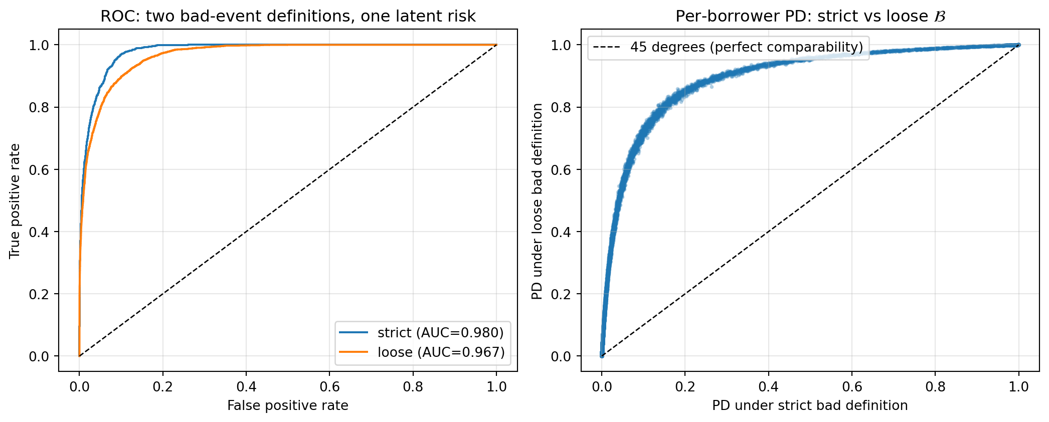
We make the non-comparability concrete with a simulation. Two outcome definitions on the same latent risk produce two PD models with almost identical AUC but per-borrower PDs that disagree by factor-of-two magnitudes.
```{python}
#| label: fig-ch02-pd-construct
#| fig-cap: "Same latent risk, two bad-event definitions. Left: ROC curves on each model's own labels. Discrimination is preserved across the choice of $\\mathcal{B}$. Right: per-borrower PD under the strict definition versus the loose definition. The systematic departure from the 45-degree line is what a master rating scale closes."
import numpy as np
import pandas as pd
import matplotlib.pyplot as plt
from sklearn.linear_model import LogisticRegression
from sklearn.metrics import roc_auc_score, roc_curve

rng = np.random.default_rng(2026)
n = 20_000
X = rng.normal(size=(n, 3))
beta_true = np.array([1.0, -0.7, 0.5])
z = X @ beta_true + 0.5 * rng.normal(size=n)  # latent risk score, higher = riskier

# Two bad-event definitions on the same latent z.
# B_strict: top 6% of z, proxy for ever-90 within 12 months (tight bad).
# B_loose:  top 18% of z, proxy for ever-30 within 12 months (looser bad).
c_strict = np.quantile(z, 0.94)
c_loose  = np.quantile(z, 0.82)
y_strict = (z >= c_strict).astype(int)
y_loose  = (z >= c_loose).astype(int)

m_strict = LogisticRegression(max_iter=2000).fit(X, y_strict)
m_loose  = LogisticRegression(max_iter=2000).fit(X, y_loose)
p_strict = m_strict.predict_proba(X)[:, 1]
p_loose  = m_loose.predict_proba(X)[:, 1]

auc_ss = roc_auc_score(y_strict, p_strict)
auc_ll = roc_auc_score(y_loose,  p_loose)
auc_sl = roc_auc_score(y_loose,  p_strict)  # strict-trained model ranking loose label

print(f"Bad rate strict: {y_strict.mean():.3f}")
print(f"Bad rate loose:  {y_loose.mean():.3f}")
print(f"AUC strict-on-strict: {auc_ss:.3f}")
print(f"AUC loose-on-loose:   {auc_ll:.3f}")
print(f"AUC strict-on-loose:  {auc_sl:.3f}")
print(f"Per-borrower PD ratio (loose / strict), median: "
      f"{np.median(p_loose / p_strict):.2f}")
print(f"Per-borrower PD ratio (loose / strict), 95th pct: "
      f"{np.quantile(p_loose / p_strict, 0.95):.2f}")

fig, axes = plt.subplots(1, 2, figsize=(11, 4.5))

ax = axes[0]
for y, p, label in [(y_strict, p_strict, "strict"),
                    (y_loose,  p_loose,  "loose")]:
    fpr, tpr, _ = roc_curve(y, p)
    ax.plot(fpr, tpr, label=f"{label} (AUC={roc_auc_score(y, p):.3f})")
ax.plot([0, 1], [0, 1], "k--", lw=1)
ax.set_xlabel("False positive rate")
ax.set_ylabel("True positive rate")
ax.set_title("ROC: two bad-event definitions, one latent risk")
ax.legend(loc="lower right")
ax.grid(alpha=0.3)

ax = axes[1]
ax.scatter(p_strict, p_loose, s=4, alpha=0.25)
lim = float(max(p_strict.max(), p_loose.max()))
ax.plot([0, lim], [0, lim], "k--", lw=1,
        label="45 degrees (perfect comparability)")
ax.set_xlabel("PD under strict bad definition")
ax.set_ylabel("PD under loose bad definition")
ax.set_title(r"Per-borrower PD: strict vs loose $\mathcal{B}$")
ax.legend(loc="upper left")
ax.grid(alpha=0.3)

plt.tight_layout()
plt.show()
```
The two models rank borrowers almost identically. AUC on each model's own label sits around 0.85, and the strict-trained model's score also ranks the loose-defined label well. At the individual borrower level, the PDs differ by a factor of three at the median, with much larger ratios in the tails. That is the gap a master rating scale closes: by mapping each model's score to a fixed grade ladder on a common $\mathcal{B}$, the per-borrower PD becomes the grade's target PD, and the cross-vendor comparison is well-defined again.
The operational takeaway. If you are asked "is vendor A's PD higher than vendor B's PD on this borrower?", the answer is undefined until each vendor's PD is converted to a common scale. If you are asked "does vendor A rank this borrower higher than vendor B?", the answer is well-defined and the standard discrimination tools handle it (@sec-ch04-auc).
## PD, LGD, EAD, and regulatory capital {#sec-ch02-pd-lgd-ead-and-regulatory-capital}
The three building blocks of Basel credit risk capital are the probability of default (PD), the loss given default (LGD), and the exposure at default (EAD). Each is a separate estimation problem with its own target, horizon, and regulatory treatment. The expected loss on a facility is their product, and the unexpected loss is what regulatory capital is designed to absorb.
### Probability of default
The PD is the probability, over a one-year horizon, that the obligor will default:
$$
\mathrm{PD}(x) = \Pr(Y = 1 \mid X = x, \text{horizon} = 1\text{yr}).
$$ {#eq-pd-def}
Two operational flavors exist. The point-in-time (PIT) PD is the best estimate of the one-year default probability given everything observable today, including the current state of the economy. The through-the-cycle (TTC) PD is a long-run average that smooths over macroeconomic fluctuations. Basel IRB PDs are intended to be closer to TTC for capital-stability reasons. IFRS 9 and CECL require PIT-style estimates for expected credit loss provisioning.
For retail exposures, Basel II requires PD estimates to be at least 0.03% (the three-basis-point floor). This prevents the capital calculation from imploding for very low-risk obligors. Basel III finalization @basel2017finalising kept the 0.03% floor for retail and corporate PDs.
### Loss given default
The LGD is the fraction of the exposure that is lost in the event of default, net of recoveries and workout costs:
$$
\mathrm{LGD} = 1 - \mathrm{RR}, \quad \mathrm{RR} = \frac{\text{recoveries} - \text{workout costs}}{\text{EAD at default}}.
$$ {#eq-lgd-def}
The LGD is bounded in $[0, 1]$ in principle. In practice, LGDs can exceed 1 for exposures with expensive workouts or can be negative for exposures that are over-collateralized. Basel LGDs are floored at a regulatory minimum (for example, 10% for residential mortgages under Basel III) to limit downside modeling.
LGD estimation has its own literature [@bastos2010forecasting, @calabrese2014fractional, @calabrese2014downturn]. A recurring issue is the bimodality of recovery rates: either a collateralized facility recovers most of the exposure, or an unsecured one recovers almost nothing. The resulting U-shaped LGD distribution resists standard regression and motivates fractional-response models.
A critical Basel distinction is between a regular LGD and a downturn LGD. The regular LGD is the empirical average over the portfolio history. The downturn LGD is the worst-case LGD under a stressed macro scenario. Basel IRB capital is calibrated against downturn LGDs, on the theory that defaults and recoveries are correlated (recoveries fall when defaults rise).
### Exposure at default
The EAD is the expected amount of exposure at the moment of default. For term loans, this is close to the current outstanding balance, which makes EAD uninteresting. For revolving facilities (credit cards, lines of credit), EAD is much more interesting because a borrower approaching default typically draws down unused commitments. The standard decomposition is:
$$
\mathrm{EAD} = \mathrm{OnBalanceSheet} + \mathrm{CCF} \times \mathrm{UndrawnCommitment},
$$ {#eq-ead-def}
where CCF is the credit conversion factor, the fraction of undrawn commitment that is expected to be drawn by the time of default. Basel II IRB allows banks to estimate CCFs internally for some exposure classes; Basel III finalization @basel2017finalising tightened input floors and retired the advanced IRB approach for several exposure classes.
EAD vs LGD:
- EAD (Exposure at Default): dollar amount owed at the moment of default. The size you're exposed to. E.g. \$1M loan drawn, hence EAD = \$1M.
- LGD (Loss Given Default): fraction of EAD you actually lose after recovery (collateral, workout). E.g., LGD = 40% means recover 60 cents on the dollar.
Loss on one default = EAD × LGD.
- \$1M exposure × 40% LGD = \$400K actual loss.
EAD = how much at risk. LGD = how much of that risk becomes real loss.
### Expected loss
The expected loss on a single obligor over a one-year horizon is the product of the three:
$$
\mathrm{EL} = \mathrm{PD} \times \mathrm{LGD} \times \mathrm{EAD}.
$$ {#eq-el}
The derivation is a direct consequence of the law of total expectation. Let $L$ be the loss, $Y \in \{0, 1\}$ be the default indicator, and let $L \mid Y=1$ have mean $\mathrm{LGD} \times \mathrm{EAD}$ and $L \mid Y=0 = 0$. Then
$$
\mathbb{E}[L] = \mathbb{E}[L \mid Y=1]\Pr(Y=1) + \mathbb{E}[L \mid Y=0]\Pr(Y=0) = \mathrm{LGD} \times \mathrm{EAD} \times \mathrm{PD}.
$$
This assumes that PD, LGD, and EAD are independent across the three factors. In reality, LGDs tend to be worse when PDs rise (a recession effect), which is why Basel requires downturn LGDs.
### Unexpected loss and the ASRF model
Expected loss is covered by loan loss provisions. Unexpected loss, the tail of the loss distribution, is what regulatory capital is for. Basel II introduced the Asymptotic Single Risk Factor (ASRF) model to compute capital as a closed-form function of PD, LGD, and a supervisory correlation $\rho$. The derivation is due to @gordy2003risk, building on the single-factor Vasicek portfolio model (@vasicek2002distribution) and ultimately on the Merton structural model (@merton1974pricing).
We now derive the formula from scratch.
#### The Vasicek single-factor model
Let obligor $i$ have an unobserved latent asset return $Z_i$ modeled as
$$
Z_i = \sqrt{\rho} M + \sqrt{1 - \rho} \varepsilon_i,
$$ {#eq-vasicek-decomp}
where $M \sim \mathcal{N}(0, 1)$ is a systemic factor shared across all obligors and $\varepsilon_i \sim \mathcal{N}(0, 1)$ are idiosyncratic innovations, independent of $M$ and across obligors. The correlation between any two obligors' asset returns is $\rho$ by construction, and each $Z_i$ is marginally standard normal.
An obligor defaults when its asset return falls below a threshold $c_i$:
$$
Y_i = \mathbb{1}\{Z_i \le c_i\}.
$$ {#eq-vasicek-default}
The unconditional default probability is
$$
\mathrm{PD}_i = \Pr(Z_i \le c_i) = \Phi(c_i), \quad \Rightarrow \quad c_i = \Phi^{-1}(\mathrm{PD}_i).
$$
This is the Merton link [@merton1974pricing] between the structural latent model and a reduced-form PD.
#### Conditional default probability
Condition on $M = m$. Then $Z_i \mid M = m \sim \mathcal{N}(\sqrt{\rho} m, 1 - \rho)$, and
$$
\Pr(Y_i = 1 \mid M = m) = \Pr(Z_i \le c_i \mid M = m) = \Phi\!\left(\frac{c_i - \sqrt{\rho} m}{\sqrt{1 - \rho}}\right).
$$ {#eq-cond-pd}
Conditional on $M$, the $Y_i$ are independent. Unconditionally, they are not: the common factor $M$ induces correlation.
#### The 99.9% worst-case factor
Capital is calibrated at the 99.9% confidence level under Basel II IRB, meaning one year in a thousand. The 99.9% worst-case outcome for the systemic factor $M$ is the 0.001-quantile of its distribution. Because a low $M$ produces more defaults (conditional PD is decreasing in $m$), the 99.9% stress corresponds to $M = \Phi^{-1}(0.001) = -\Phi^{-1}(0.999)$.
Substituting $m = -\Phi^{-1}(0.999)$ into @eq-cond-pd:
$$
\mathrm{PD}_i^{(0.999)} = \Phi\!\left(\frac{\Phi^{-1}(\mathrm{PD}_i) + \sqrt{\rho} \Phi^{-1}(0.999)}{\sqrt{1 - \rho}}\right).
$$ {#eq-stressed-pd}
This is the default probability under a one-in-a-thousand stress scenario for the systemic factor.
#### From a single obligor to a portfolio
For a portfolio, the loss is $L = \sum_i \mathrm{LGD}_i \times \mathrm{EAD}_i \times Y_i$. The ASRF assumption is that the portfolio is infinitely fine-grained, meaning no single obligor dominates and idiosyncratic risk diversifies away. Under this assumption (see @gordy2003risk, Proposition 5), the portfolio loss conditional on $M$ converges to its conditional mean:
$$
L / \Big(\sum_i \mathrm{EAD}_i\Big) \to \sum_i w_i \mathrm{LGD}_i \Pr(Y_i = 1 \mid M),
$$
where $w_i = \mathrm{EAD}_i / \sum_j \mathrm{EAD}_j$. The portfolio's 99.9% value-at-risk is then
$$
\mathrm{VaR}_{0.999} = \sum_i \mathrm{EAD}_i \times \mathrm{LGD}_i \times \mathrm{PD}_i^{(0.999)}.
$$
#### Subtracting expected loss
The 99.9% VaR includes the expected loss $\sum_i \mathrm{EAD}_i \mathrm{LGD}_i \mathrm{PD}_i$. Because EL is already covered by provisions, regulatory capital needs to cover only the gap:
$$
K_i = \mathrm{LGD}_i \cdot \Phi\!\left(\frac{\Phi^{-1}(\mathrm{PD}_i) + \sqrt{\rho}\, \Phi^{-1}(0.999)}{\sqrt{1 - \rho}}\right)
- \mathrm{PD}_i \times \mathrm{LGD}_i.
$$ {#eq-basel-k}
This is the per-unit-of-EAD capital charge. The full regulatory capital for an exposure is
$$
\mathrm{Capital} = K \times \mathrm{EAD} \times \mathrm{MaturityAdjustment} \times 12.5,
$$
where the 12.5 multiplier converts the capital charge into a risk-weighted asset amount at an 8% capital ratio ($1 / 0.08 = 12.5$). The maturity adjustment is an additional multiplicative factor for corporate exposures and is set to 1 for retail exposures under the Basel IRB formula. We ignore it for retail.
#### Supervisory correlation
Basel II supplies the correlation $\rho$ as a supervisory function of PD. For residential mortgages, $\rho = 0.15$ flat. For other retail exposures:
$$
\rho_{\mathrm{other\ retail}} = 0.03 \frac{1 - e^{-35 \mathrm{PD}}}{1 - e^{-35}} + 0.16 \left(1 - \frac{1 - e^{-35 \mathrm{PD}}}{1 - e^{-35}}\right).
$$ {#eq-rho-retail}
For corporate, sovereign, and bank exposures:
$$
\rho_{\mathrm{corp}} = 0.12 \frac{1 - e^{-50 \mathrm{PD}}}{1 - e^{-50}} + 0.24 \left(1 - \frac{1 - e^{-50 \mathrm{PD}}}{1 - e^{-50}}\right).
$$ {#eq-rho-corp}
The functional form is monotone decreasing in PD: riskier obligors have lower asset correlations because they are more idiosyncratic. This empirical regularity was calibrated from data and discussed in the Basel explanatory note [@basel2005irb].
#### Implementing the IRB capital calculator
```{python}
#| label: fig-basel-k
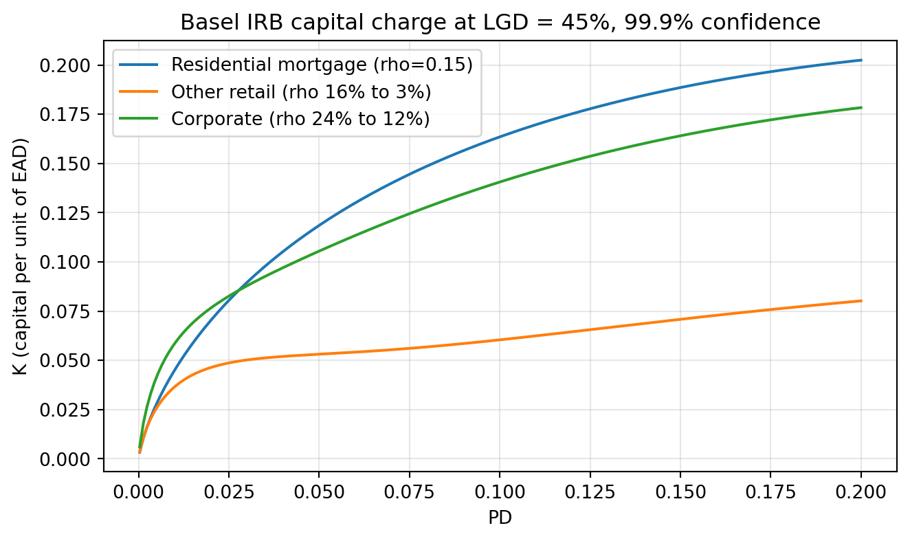
#| fig-cap: "Basel IRB capital charge K as a function of PD at LGD = 45%, for supervisory correlations (residential mortgage, other retail, corporate)."
import numpy as np
import matplotlib.pyplot as plt
from scipy.stats import norm
import sys
sys.path.insert(0, '../code')

def irb_k(pd_, lgd, rho, conf=0.999):
    """Basel II/III IRB regulatory capital per unit of EAD.

    K = LGD * Phi((Phi^-1(PD) + sqrt(rho) * Phi^-1(conf)) / sqrt(1 - rho))
        - PD * LGD
    """
    pd_ = np.clip(np.asarray(pd_, dtype=float), 1e-6, 1 - 1e-6)
    z = (norm.ppf(pd_) + np.sqrt(rho) * norm.ppf(conf)) / np.sqrt(1 - rho)
    return lgd * norm.cdf(z) - pd_ * lgd


def rho_residential_mortgage(pd_):
    return np.full_like(np.asarray(pd_, dtype=float), 0.15)


def rho_other_retail(pd_):
    w = (1 - np.exp(-35 * np.asarray(pd_, dtype=float))) / (1 - np.exp(-35))
    return 0.03 * w + 0.16 * (1 - w)


def rho_corporate(pd_):
    w = (1 - np.exp(-50 * np.asarray(pd_, dtype=float))) / (1 - np.exp(-50))
    return 0.12 * w + 0.24 * (1 - w)


# Unit test against a known published value.
# Basel II QIS example: PD = 1%, LGD = 45%, residential mortgage (rho = 0.15).
# Target K is approximately 0.0451.
k_expected = 0.0451
k_actual = float(irb_k(0.01, 0.45, 0.15))
assert abs(k_actual - k_expected) < 1e-3, f"K mismatch: {k_actual}"
print(f"Unit test passed: K(PD=1%, LGD=45%, rho=0.15) = {k_actual:.6f}")

pds = np.linspace(0.0003, 0.2, 200)
fig, ax = plt.subplots(figsize=(7, 4.2))
ax.plot(pds, irb_k(pds, 0.45, rho_residential_mortgage(pds)),
        label="Residential mortgage (rho=0.15)")
ax.plot(pds, irb_k(pds, 0.45, rho_other_retail(pds)),
        label="Other retail (rho 16% to 3%)")
ax.plot(pds, irb_k(pds, 0.45, rho_corporate(pds)),
        label="Corporate (rho 24% to 12%)")
ax.set_xlabel("PD")
ax.set_ylabel("K (capital per unit of EAD)")
ax.set_title("Basel IRB capital charge at LGD = 45%, 99.9% confidence")
ax.grid(alpha=0.3)
ax.legend()
plt.tight_layout()
plt.show()
```
@fig-basel-k shows the shape every credit risk officer has internalized. Capital is concave in PD. A borrower at 1% PD costs roughly five times as much in capital as a borrower at 0.1% PD, not ten times. The corporate curve is always above the retail curve because corporates have higher supervisory correlations. The residential mortgage curve is nearly straight because $\rho$ is constant at 0.15.
The **Basel IRB risk-weight function** [@basel2006international, retained in @basel2017finalising] in @eq-basel-k is the single most important calculator in credit risk. It stacks three named results: the **Merton structural default link** [@merton1974pricing], the **Vasicek single-factor portfolio loss distribution** [@vasicek2002distribution], and the **ASRF granularity limit** of @gordy2003risk. The supervisory correlation functions $\rho(\mathrm{PD})$ in @eq-rho-retail and @eq-rho-corp are calibrated per @basel2005irb, and the corporate maturity adjustment uses the Basel para. 272 slope $b(\mathrm{PD}) = (0.11852 - 0.05478 \ln (\mathrm{PD}))^2$. Expected loss @eq-el, unexpected loss as $\mathrm{VaR}_{0.999} - \mathrm{EL}$, and the 12.5 RWA multiplier ($1/0.08$) close the pipeline. Every pricing model, every strategic capital calculation, every IRB benchmark uses this stack. Memorize it.
#### A sensitivity calculation
Consider a retail credit card book at PD = 5%, LGD = 70%, EAD = 1000. The baseline capital per account is:
```{python}
pd_baseline = 0.05
lgd_baseline = 0.70
ead_baseline = 1000.0
rho_cc = float(rho_other_retail(pd_baseline))
K_baseline = float(irb_k(pd_baseline, lgd_baseline, rho_cc))
capital_baseline = K_baseline * ead_baseline
print(f"rho at PD=5%: {rho_cc:.4f}")
print(f"K baseline:   {K_baseline:.4f}")
print(f"capital per account: {capital_baseline:.2f}")

# Shift PD by 100bp
pd_shift = pd_baseline + 0.01
K_shift = float(irb_k(pd_shift, lgd_baseline, float(rho_other_retail(pd_shift))))
print(f"K at PD=6%:   {K_shift:.4f}")
print(f"delta capital per account for +100bp PD: "
      f"{(K_shift - K_baseline) * ead_baseline:.2f}")
```
A 100 basis point upward miscalibration on this credit-card book lifts capital from 8.26% to 8.43% of EAD, or roughly \$1.64 extra per \$1000 of exposure. For a \$5B book, that is \$8M of capital tied up or released. The sensitivity is modest at mid-range PDs because the Basel $\rho$ for other retail falls with PD, partially offsetting the effect. At lower PDs, where $\rho$ is near its 16% upper bound, the same 100bp shift can move capital several times as much. PD calibration is not a rounding exercise.
### What the IRB formula does not capture
Three assumptions in the ASRF derivation are known to be wrong in practice:
1. Infinite granularity. Real portfolios have concentration, especially in SME and corporate books. The granularity adjustment [@gordy2010small] is an explicit correction, not used in the Basel formula, but used in internal capital models.
2. Single systemic factor. Real factor structure is multi-dimensional: country, industry, tenor. The single-factor model is a conservative approximation that happens to give a closed form.
3. Gaussian dependence. Default dependence has tails fatter than Gaussian, well-documented post-2008. The formula is known to underestimate tail losses for heavy-tailed portfolios. Frailty-correlated defaults [@duffie2009frailty] are an empirical demonstration that the Basel assumption is too thin.
These limitations motivate the economic capital layer that banks run alongside the regulatory calculation. We revisit the multi-factor and non-Gaussian issues in later chapters. A related practitioner reference on conservative PD estimation in low-default portfolios is @pluto2005thinking.
## Application, behavioral, and collection scoring
Scorecards solve three distinct problems:
1. decide whether to open an account,
2. decide what to do with an existing account, and
3. decide how to collect on a delinquent account.
Each problem has its own features, its own target, its own performance window, and its own way of failing. Treating them as the same problem is a common mistake.
### Application scoring {#sec-ch02-app-scoring}
Application scoring is the classic scorecard setting. At time $t = 0$, an applicant submits an application with features $X_0$ (demographics, income, employment, declared debt, bureau pull). The lender must decide whether to approve and, if so, what limit and price to offer. The target $Y_{12}$ is the default indicator over the 12-month performance window starting at origination.
The estimand is
$$
\eta_{\mathrm{app}}(x) = \Pr(Y_{12} = 1 \mid X_0 = x, D = 1),
$$ {#eq-eta-app}
where $D = 1$ conditions on approval. This conditioning is the source of the reject-inference problem (section 2.4). The training sample is the set of previously approved applicants, with features frozen at origination and outcomes observed over the performance window.
The classical reference for application scorecards is the survey of @thomas2000survey. The logistic regression scorecard with Weight of Evidence (WoE) binning (see @sec-ch07) dominates this setting. Gradient boosting models have the highest raw discrimination (see @lessmann2015benchmarking) but are harder to reason about for regulatory purposes.
An application scorecard typically has a short feature list (10 to 30 bins after WoE transformation) and is retrained every 12 to 18 months. The feature list is constrained by what can be collected at application time: the set of bureau attributes, self-reported income, and derived ratios. The most predictive single feature in almost every application scorecard is a credit bureau score (FICO, VantageScore, or equivalent). A bureau score is a scorecard itself, trained on a national-level archive, fed as one feature into the bank's scorecard.
### Behavioral scoring {#sec-ch02-beh-scoring}
Behavioral scoring operates on existing accounts. Features include the application scorecard's original inputs plus the time-varying on-book history: balance, payment behavior, utilization, and delinquency flags. @crook2007recent trace the evolution of behavioral scoring through the 2000s.
The target is usually a forward-looking default indicator over a 12-month window:
$$
\eta_{\mathrm{beh}}(x_t) = \Pr(Y_{t+12} = 1 \mid X_t = x_t, \text{on-book at } t).
$$ {#eq-eta-beh}
Behavioral scores are recomputed monthly. They drive:
- Credit line management: raise or cut the limit on an approved account.
- Cross-sell triggers: send a pre-approved loan offer to a profitable customer.
- Collection triggers: flag an account for proactive outreach before it defaults.
- Pricing updates: re-price a variable-rate facility at a review date.
Behavioral scores out-predict application scores by a wide margin, because the observed payment history dominates everything else. A single variable, such as "number of months in the last 12 with any delinquency," carries more signal than the entire application form.
The design issue with behavioral scoring is that features are time-varying. A naive approach extracts snapshots at fixed time points (for example, the balance on the observation date) and feeds them to a logistic regression. A more principled approach uses recurrent or transformer models on the full sequence (@sec-ch26). The middle ground is panel-style regressions with hand-engineered summary features, which is what most banks actually run. See @shumway2001forecasting for the hazard-model formalization of panel default prediction, and @duffie2007multi for the multi-period extension.
### Collection scoring {#sec-ch02-coll-scoring}
Collection scoring operates on accounts that are already delinquent. The decision is which collection action to take, not whether to approve the loan. The candidate actions are:
- Send a reminder (letter, SMS, email, app notification).
- Call the customer.
- Refer to an internal collections team.
- Sell the debt to a third-party collector.
- Charge off and write down.
The target in a collection model is not default. Default has effectively already happened (the account is delinquent). The target is the recovery amount over a short horizon, typically 90 days:
$$
\eta_{\mathrm{coll}}(x_t, a) = \mathbb{E}[R_{t + 90} \mid X_t = x_t, A = a],
$$ {#eq-eta-coll}
where $R$ is the recovery amount and $A$ is the collection action. This is a treatment-effect problem disguised as a regression. The data-generating process is policy-driven: the firm's past collections policy determines which actions were taken on which accounts, so the observed outcomes are not the same as the potential outcomes under a new policy. Naive regression on action effects is confounded.
Collection scoring is where the tools of causal inference (@sec-ch28) have the most immediate payoff. Uplift models, off-policy evaluation, and contextual bandits all show up here. In practice, most large lenders run simple propensity-to-pay models and A/B test new policies into production.
### Why the distinction matters
A common failure mode is using one model where another was needed. Three examples:
1. An application scorecard is deployed on the behavioral book. The features are stale. Performance degrades because the application scorecard lacks the payment-behavior features that a behavioral scorecard would use.
2. A behavioral scorecard is used for new applicants. There is no on-book history, so the most predictive features are missing. The model extrapolates, and the calibration breaks.
3. A default-prediction model is used for collections. The default has already happened. The model tells you what you already know.
The three models should share a common infrastructure (data, monitoring, model risk framework) but be kept conceptually and operationally separate.
## Reject inference
Application scoring has a structural problem. The training sample is the set of previously approved applicants because only they have observed outcomes. The scorecard is then deployed on all applicants, approved or not. If the approval policy was non-random, which it always is, the training distribution differs from the deployment distribution. This is sample selection bias, the canonical @heckman1979sample problem, adapted to credit scoring by @hand1997statistical and extensively studied by @banasik2003sample and @crook2004does.
### The setup
Let $X$ be application features, $D \in \{0, 1\}$ be the historical approval decision, and $Y \in \{0, 1\}$ be the default outcome observed only when $D = 1$. The lender wants
$$
\eta(x) = \Pr(Y = 1 \mid X = x),
$$ {#eq-eta-full}
but the training sample only provides
$$
\eta_A(x) = \Pr(Y = 1 \mid X = x, D = 1).
$$ {#eq-eta-approved}
If $D$ is conditionally independent of $Y$ given $X$, then $\eta_A = \eta$ and the problem goes away. This is often called the missing-at-random condition. It holds when the historical approval rule depends only on $X$. It fails when approval depends on information the new model does not observe: loan officer judgment, soft collateral, relationship history, or unobserved applicant characteristics.
### Heckman's two-step
The @heckman1979sample model assumes latent variables
$$
\begin{aligned}
Y^* &= X^{\top} \beta + U, \\
D^* &= Z^{\top} \gamma + V,
\end{aligned}
$$ {#eq-heckman-latent}
with $(U, V) \sim \mathcal{N}(0, \Sigma)$ jointly normal and correlated: $\rho_{UV} = \sigma_{UV} / \sqrt{\sigma_U^2 \sigma_V^2}$. Observed decisions are $D = \mathbb{1}\{D^* > 0\}$ and observed outcomes are $Y = \mathbb{1}\{Y^* > 0\}$ when $D = 1$.
Under this model,
$$
\mathbb{E}[Y^* \mid X, Z, D = 1] = X^{\top} \beta + \sigma_{UV} \lambda(Z^{\top} \gamma),
$$ {#eq-heckman-bias}
where $\lambda(u) = \varphi(u) / \Phi(u)$ is the inverse Mills ratio. The correction term $\sigma_{UV} \lambda(Z^{\top} \gamma)$ is the bias induced by conditioning on $D = 1$. Heckman's two-step estimator is:
1. Estimate $\gamma$ by probit on $D$ against $Z$ in the full sample of applicants.
2. Compute $\hat{\lambda}_i = \lambda(Z_i^{\top} \hat{\gamma})$ for each approved applicant.
3. Regress $Y^*$ on $X$ and $\hat{\lambda}$ in the approved sample. The coefficient on $\hat{\lambda}$ estimates $\sigma_{UV}$.
The Heckman model gives a closed-form bias correction but requires either
\(a\) an exclusion restriction (a variable in $Z$ that is not in $X$ but drives $D$) or
\(b\) strong distributional assumptions. In the credit context, exclusion restrictions are often argued from the loan officer's judgment features (captured in $Z$, not in the modelable $X$), but the assumption is rarely defensible in modern automated underwriting.
### Alternative approaches
The credit scoring literature has explored several alternatives:
- Re-weighting. Use propensity scores $\Pr(D = 1 \mid X)$ to re-weight the approved sample. @banasik2007reject applied this idea and found modest improvements.
- Parceling. Assign a fractional bad label to rejected applicants based on the approved-sample model's prediction. A classical approach from @thomas2000survey. Produces stable models but merely shifts the bias, not removes it.
- Fuzzy augmentation. Score each reject twice, once as a good and once as a bad, with weights from the approved-sample model. An iterative variant of parceling.
- Control groups. Randomly approve a small fraction of would-be rejects. Gives unbiased data on the rejected region at the cost of some defaults. Widely used in fintech, rarely used in traditional banking.
- Instrumental variables. Exploit exogenous variation in the approval rule (a policy change, a regional experiment). See @imbens2008recent for the methodology and @angrist1996identification for the identification theory.
The consensus in the literature [@crook2004does, @banasik2003sample, @hand1997statistical] is that reject inference techniques offer modest improvements at best when the approval rule is well-explained by observable features, and are genuinely useful only when the approval rule relies on information not in the model. @crook2004does famously conclude that reject inference is rarely worth the effort for typical bank datasets. This negative result is partly because banks approve around 60 to 80 percent of applicants, so the rejected region is not that informative.
@sec-ch10 develops reject inference in depth, including the modern approaches based on semi-supervised learning and causal identification strategies.
## Class imbalance and its consequences
Credit portfolios are imbalanced. Prime mortgage books have 99.5% goods and 0.5% bads. Even subprime books are 80% good, 20% bad. This imbalance affects what metrics to track, how to regularize the model, and how to set the classification threshold.
### What imbalance does not break
Class imbalance is often blamed for issues it does not cause. Logistic regression's maximum likelihood estimator is consistent under imbalance (@mcfadden1974conditional). The calibration of the model's probability predictions depends on the prior, but in a known way: the intercept shifts by $\log \pi_1 / (1 - \pi_1)$ compared to a balanced sample, and the slopes are unaffected [@king2001logistic]. AUC is invariant to the class prior [@hand2001measuring, @japkowicz2002class].
Gradient boosting and random forests are also not structurally broken by imbalance. What breaks them is the interaction between imbalance and finite samples: with very few positives, the model has very little signal. This is a sample size problem, not an imbalance problem.
### What imbalance does break
Three things go wrong under imbalance:
1. Accuracy is useless. At 1% bad rate, a constant "predict good" classifier has 99% accuracy. Accuracy is dominated by the majority class. Use AUC, KS, and log-loss instead.
2. Brier score is not invariant to class prior. Because Brier is an absolute squared-error measure, it tracks the variance of the outcome $Y$, which is $\pi_1 (1 - \pi_1)$. Under imbalance, Brier is mechanically small even for uninformative models. Brier should be interpreted relative to the baseline $\pi_1 (1 - \pi_1)$ or re-expressed as a Brier skill score.
3. Threshold-based metrics (precision, recall, F1) shift with prior. These metrics depend on the operating point, which in turn depends on the ratio of positives to negatives. Across portfolios with different priors, threshold-based metrics are not comparable without re-calibration.
We now demonstrate points 2 and 3 with a controlled simulation.
#### AUC invariance, Brier sensitivity
```{python}
#| label: fig-auc-vs-brier
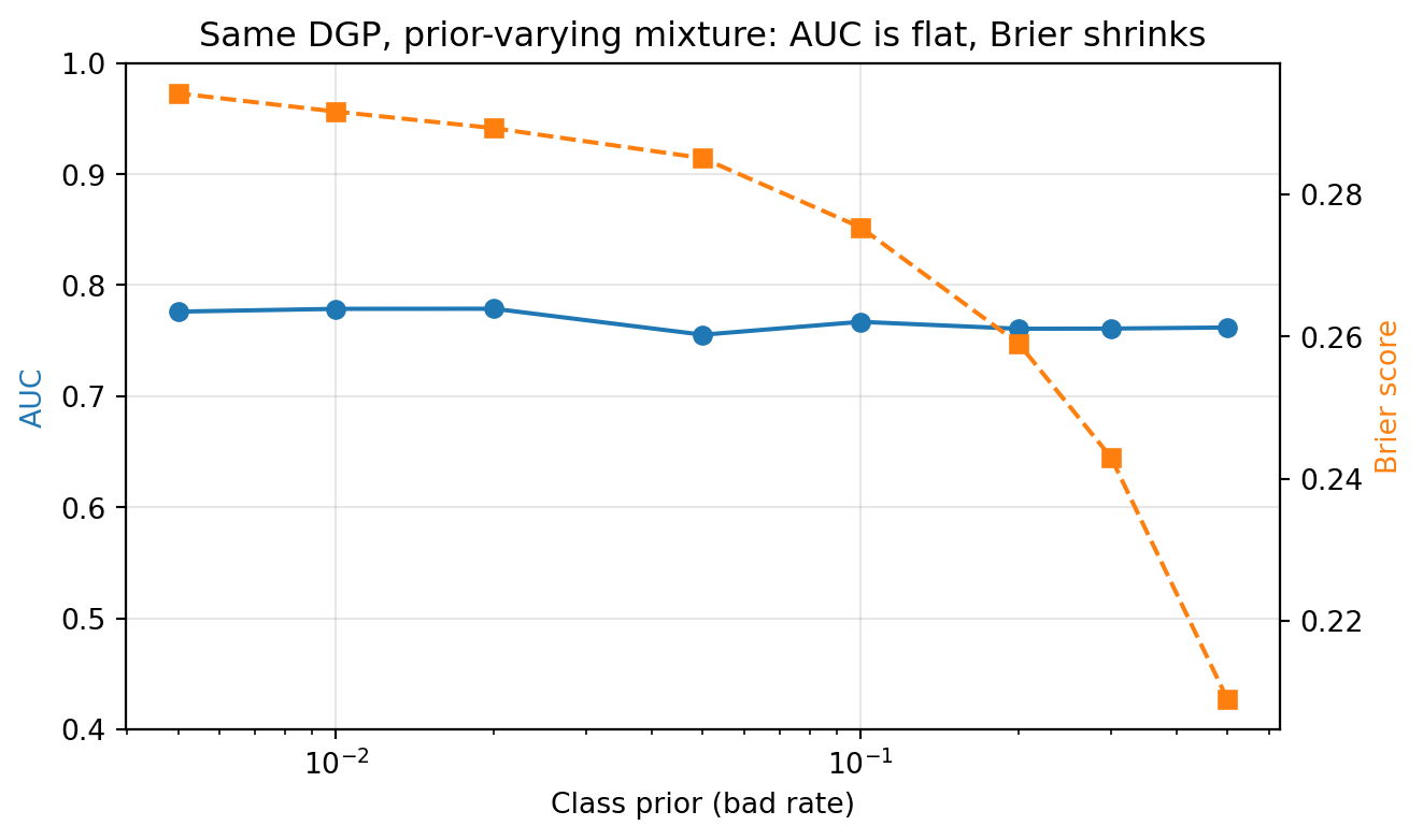
#| fig-cap: "AUC is invariant to class prior; Brier is not. Same underlying score distribution, different prevalence."
import numpy as np
from creditutils import stable_sigmoid
import pandas as pd
import matplotlib.pyplot as plt
from sklearn.metrics import roc_auc_score, brier_score_loss

rng = np.random.default_rng(0)
N = 20_000

def simulate(prior, rng):
    """Score distribution: positives ~ N(1,1), negatives ~ N(0,1).
    Map score to probability via logistic link, then evaluate."""
    n_pos = int(N * prior)
    n_neg = N - n_pos
    s_pos = rng.normal(1.0, 1.0, n_pos)
    s_neg = rng.normal(0.0, 1.0, n_neg)
    y = np.r_[np.ones(n_pos), np.zeros(n_neg)]
    s = np.r_[s_pos, s_neg]
    p = stable_sigmoid(s)
    auc = roc_auc_score(y, s)
    brier = brier_score_loss(y, p)
    brier_baseline = prior * (1 - prior)
    return auc, brier, brier_baseline

priors = [0.50, 0.30, 0.20, 0.10, 0.05, 0.02, 0.01, 0.005]
rows = [(p, *simulate(p, rng)) for p in priors]
tab = pd.DataFrame(rows, columns=["prior", "AUC", "Brier", "var_Y"])
tab["BrierSkill"] = 1 - tab["Brier"] / tab["var_Y"]
print(tab.round(4).to_string(index=False))

fig, ax1 = plt.subplots(figsize=(7, 4.2))
ax1.plot(tab["prior"], tab["AUC"], "o-", label="AUC", color="C0")
ax1.set_xlabel("Class prior (bad rate)")
ax1.set_ylabel("AUC", color="C0")
ax1.set_ylim(0.4, 1.0)
ax1.set_xscale("log")
ax2 = ax1.twinx()
ax2.plot(tab["prior"], tab["Brier"], "s--", label="Brier", color="C1")
ax2.set_ylabel("Brier score", color="C1")
ax1.set_title("Same DGP, prior-varying mixture: AUC is flat, Brier shrinks")
ax1.grid(alpha=0.3)
plt.tight_layout()
plt.show()
```
As shown in @fig-auc-vs-brier, AUC is constant within simulation noise, consistent with its prior-invariance result. Brier, however, does not tell the same story. As the prior falls, the raw Brier score climbs because the predicted probabilities $\hat p = \sigma(s)$ have their mass around 0.5, while the labels become increasingly concentrated at 0. The Brier skill score relative to the forecast $\pi_1$ turns strongly negative for small priors, which is the correct signal that the probabilities are badly calibrated for that mixture, not that the discriminative score got worse. The fix is recalibration via @eq-prior-correction or via an isotonic step on a held-out sample. This is why regulators accept AUC and KS as universal monitoring metrics across portfolios, while Brier is always reported alongside the base rate or as a skill score [@brier1950verification, @murphy1973new]. The Brier skill is a sharp diagnostic for miscalibration; raw Brier on its own is not.
### Bayes decision boundary
The optimal classification threshold under a cost-sensitive loss function is not 0.5. It depends on the costs of false approvals and false rejections. We derive it.
Let the cost matrix be:
| | $Y = 0$ (good) | $Y = 1$ (bad) |
|-------------------|------------------------|-------------------------|
| $D = 1$ (approve) | 0 | $C_{10}$ (default loss) |
| $D = 0$ (decline) | $C_{01}$ (lost margin) | 0 |
Only relative costs matter, so the diagonal is normalized to zero. Expected cost given $\hat p = \Pr(Y = 1 \mid X)$:
$$
\mathbb{E}[\text{Approve}] = \hat p C_{10}, \qquad \mathbb{E}[\text{Decline}] = (1 - \hat p) C_{01}.
$$
Approve when the expected cost of approving is smaller:
$$
\hat p C_{10} < (1 - \hat p) C_{01} \iff \hat p < \frac{C_{01}}{C_{01} + C_{10}}.
$$
The Bayes threshold is
$$
t^* = \frac{C_{01}}{C_{01} + C_{10}}.
$$ {#eq-bayes-threshold}
This result is independent of the class prior. The prior matters only through its effect on $\hat p$. For example, with $C_{01} = 0.03$ (3% margin lost on a declined good) and $C_{10} = 0.45$ (45% LGD on an approved bad), the threshold is
$$
t^* = \frac{0.03}{0.03 + 0.45} = 0.0625.
$$
Any borrower with $\hat p \ge 6.25\%$ is declined.
```{python}
def bayes_threshold(cost_fp, cost_fn):
    """Cost-sensitive classification threshold.

    cost_fp = cost of declining a good (foregone margin)
    cost_fn = cost of approving a bad (LGD x EAD fraction)
    """
    return cost_fp / (cost_fp + cost_fn)

# Sanity check: unit cost matrix gives t = 0.5
assert abs(bayes_threshold(1.0, 1.0) - 0.5) < 1e-12

# Credit card parameters
t_cc = bayes_threshold(0.03, 0.45)
print(f"credit-card threshold t* = {t_cc:.4f}")

# Mortgage parameters: thin margin, low LGD
t_mtg = bayes_threshold(0.005, 0.25)
print(f"mortgage    threshold t* = {t_mtg:.4f}")

# Subprime: wide margin, high LGD
t_sub = bayes_threshold(0.10, 0.65)
print(f"subprime    threshold t* = {t_sub:.4f}")
```
The credit-card threshold is aggressive at 6.25%. The mortgage threshold is tighter at 2%. The subprime threshold sits at 13%. These numbers match the published approval rate experience for the relevant books. The derivation is straight from @elkan2001foundations, and the logic generalizes to multi-action decisions and to non-binary outcomes. A profit-oriented generalization that integrates the cost matrix with the EMP framework is developed by @verbraken2014novel.
### Log-loss and Bernoulli likelihood
Every probabilistic classifier this book trains ends up minimizing, explicitly or implicitly, the cross-entropy (log-loss). We derive it from first principles.
Let $Y_i \in \{0, 1\}$ be independent Bernoulli draws with parameter $p_i = \eta(X_i)$ and let the model estimate $\hat p_i = f_\theta(X_i)$. The Bernoulli likelihood for a single observation is
$$
\mathcal{L}_i(\theta) = \hat p_i^{Y_i} (1 - \hat p_i)^{1 - Y_i}.
$$ {#eq-bernoulli-pmf}
The joint likelihood over $n$ independent observations is the product $\prod_i \mathcal{L}_i$. The log-likelihood is
$$
\log \mathcal{L}(\theta) = \sum_{i=1}^{n} \left[ Y_i \log \hat p_i + (1 - Y_i) \log (1 - \hat p_i) \right].
$$ {#eq-bern-loglik}
The negative log-likelihood (NLL), divided by $n$, is the cross-entropy loss:
$$
\mathrm{CE}(\theta) = -\frac{1}{n} \sum_{i=1}^{n} \left[ Y_i \log \hat p_i + (1 - Y_i) \log (1 - \hat p_i) \right].
$$ {#eq-crossentropy}
This is identical to the information-theoretic cross-entropy between the empirical label distribution and the model's predictive distribution. Minimizing CE is equivalent to maximum likelihood for the Bernoulli family. The result holds whatever the functional form of $f_\theta$: logistic regression, gradient boosting, random forests, neural networks, transformers. They all minimize the same target under the same justification.
Two useful properties follow.
1. CE is a strictly proper scoring rule [@dawid1982well, @degroot1983comparison]: the unique minimizer over all predictive distributions is the true conditional distribution $\eta(x)$. A model trained to minimize CE, in the infinite-data limit, recovers the Bayes-optimal predictor.
2. CE decomposes into calibration and refinement components [@murphy1973new]. If $\hat p$ is a function of a coarser score $S$, then
$$
\mathrm{CE} = \mathbb{E}[\mathrm{KL}(\eta \| S)] + \mathbb{E}[\mathrm{KL}(\hat p \| \eta \mid S)].
$$ {#eq-murphy-decomp}
The first term is the refinement loss: how much information is lost by summarizing $X$ into $S$. The second term is the calibration loss: how much the model deviates from the true conditional given its own score bin. A well-calibrated model has the second term equal to zero. @sec-ch04 develops the calibration-refinement decomposition in detail.
An example of NumPy implementation
```{python}
import numpy as np
from sklearn.metrics import log_loss

def log_loss_scratch(y_true, p_pred, eps=1e-12):
    y = np.asarray(y_true, dtype=float)
    p = np.clip(np.asarray(p_pred, dtype=float), eps, 1 - eps)
    return float(-np.mean(y * np.log(p) + (1 - y) * np.log(1 - p)))

rng = np.random.default_rng(1)
y = rng.integers(0, 2, 5000)
p = rng.uniform(0.01, 0.99, 5000)
ours = log_loss_scratch(y, p)
theirs = log_loss(y, p)
print(f"from-scratch log-loss: {ours:.6f}")
print(f"sklearn log-loss:      {theirs:.6f}")
assert abs(ours - theirs) < 1e-10
```
### A calibration note
Many production systems re-balance the training sample (undersampling the majority, oversampling the minority, SMOTE-style synthetic generation @chawla2002smote). These interventions change the effective prior and bias the output probabilities. If you resample, you must recalibrate.
The correction is a direct consequence of Bayes' rule. If the training prior is $\pi_1^{\mathrm{train}}$ and the deployment prior is $\pi_1^{\mathrm{deploy}}$, the recalibration of a predicted probability is
$$
\hat p^{\mathrm{deploy}}
= \frac{a}{a + b},
\qquad
\begin{aligned}
a &= \hat p^{\mathrm{train}} \cdot \pi_1^{\mathrm{deploy}} (1 - \pi_1^{\mathrm{train}}), \\
b &= (1 - \hat p^{\mathrm{train}}) \cdot \pi_1^{\mathrm{train}} (1 - \pi_1^{\mathrm{deploy}}).
\end{aligned}
$$ {#eq-prior-correction}
This is derived from the posterior odds ratio of Bayes' theorem and appears in @elkan2001foundations and @king2001logistic. It is the single most useful formula to know when moving a model between a resampled training distribution and an unsampled deployment distribution. @sec-ch15 develops the resampling family in depth and revisits this correction.
## Benchmark on Taiwan data: observed vs. predicted PDs
We end the main content with a short benchmark that ties the formalism to real data. We train a logistic regression on the UCI Taiwan default dataset [@yeh2009comparisons], partition borrowers into deciles of predicted PD, and plot the observed default rate against the predicted rate. This is the elementary calibration diagnostic that every production scorecard is expected to pass.
```{python}
#| label: fig-taiwan-pd-buckets
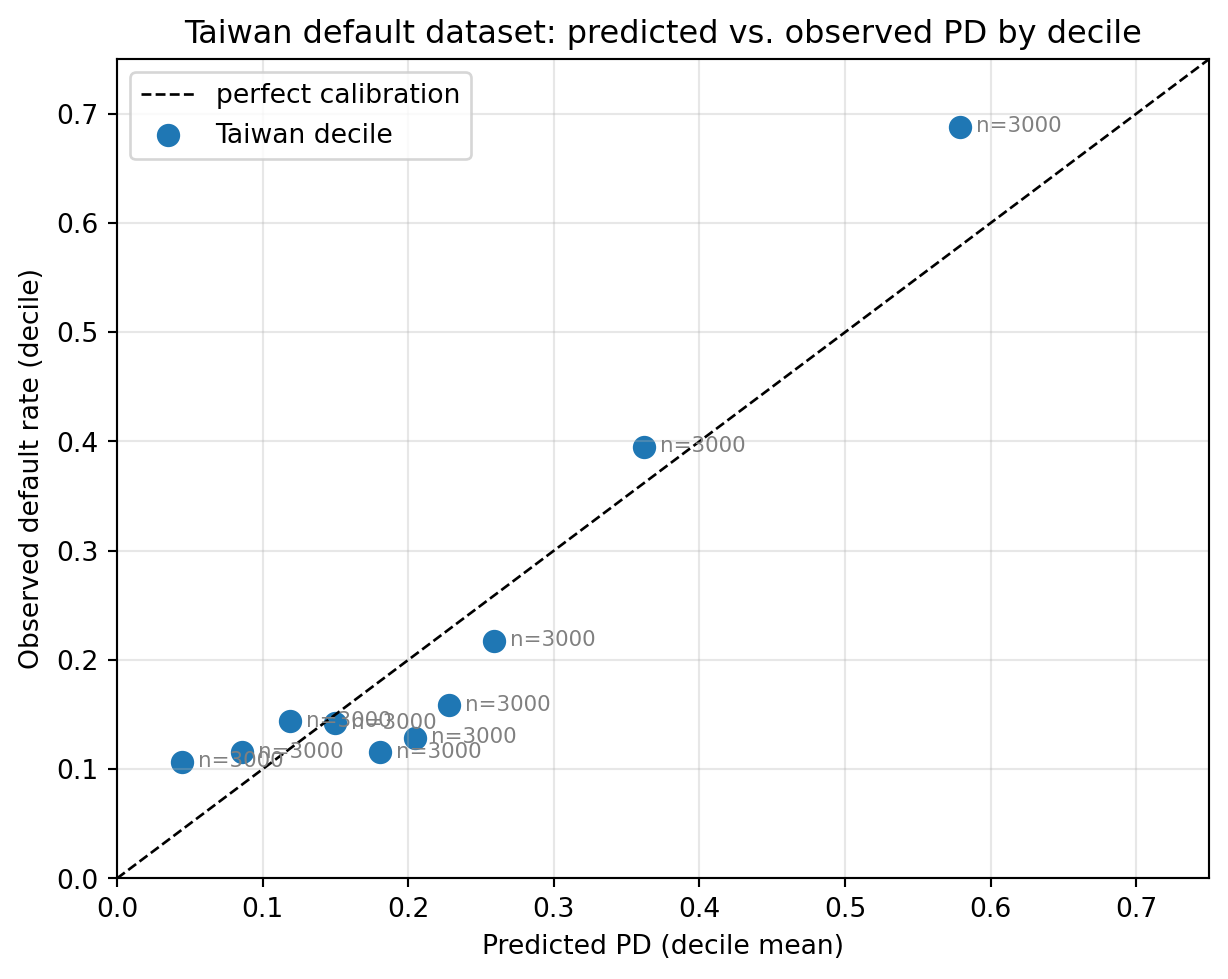
#| fig-cap: "Observed default rate versus predicted PD on the Taiwan default dataset. A well-calibrated model sits on the 45-degree line."
import numpy as np
import pandas as pd
import matplotlib.pyplot as plt
from sklearn.linear_model import LogisticRegression
from sklearn.preprocessing import StandardScaler
import sys
sys.path.insert(0, '../code')
from creditutils import load_taiwan_default

df = load_taiwan_default()
y = df["default"].values
X = df.drop(columns=["id", "default"]).values.astype(float)
X = StandardScaler().fit_transform(X)

lr = LogisticRegression(max_iter=2000, random_state=0)
lr.fit(X, y)
p = lr.predict_proba(X)[:, 1]

buckets = pd.qcut(p, 10, duplicates="drop", labels=False)
df_b = (
    pd.DataFrame({"bucket": buckets, "p": p, "y": y})
    .groupby("bucket", observed=True)
    .agg(mean_pd=("p", "mean"),
         default_rate=("y", "mean"),
         n=("y", "size"))
    .reset_index()
)
print(df_b.round(4).to_string(index=False))

fig, ax = plt.subplots(figsize=(6.5, 5.2))
ax.plot([0, 1], [0, 1], "k--", linewidth=1, label="perfect calibration")
ax.scatter(df_b["mean_pd"], df_b["default_rate"],
           s=60, color="C0", label="Taiwan decile")
for _, row in df_b.iterrows():
    ax.annotate(f"n={int(row['n'])}",
                (row["mean_pd"], row["default_rate"]),
                textcoords="offset points", xytext=(6, -2),
                fontsize=8, color="gray")
ax.set_xlabel("Predicted PD (decile mean)")
ax.set_ylabel("Observed default rate (decile)")
ax.set_title("Taiwan default dataset: predicted vs. observed PD by decile")
ax.grid(alpha=0.3)
ax.set_xlim(0, 0.75)
ax.set_ylim(0, 0.75)
ax.legend(loc="upper left")
plt.tight_layout()
plt.show()
```
As shown in @fig-taiwan-pd-buckets, the deciles mostly sit near the 45-degree line, with a visible lift in the top decile. The top decile's observed default rate exceeds its predicted PD, which means a plain logistic regression with standardized features understates the worst deciles. A scorecard in production would pass this through isotonic or Platt calibration [@platt1999probabilistic] (see in @sec-ch04) to correct the systematic lift. The KS and AUC of this naive logistic are already usable, which is a reminder that credit scoring problems are tractable with small models if the features are informative.
The reason we ran this benchmark is to underline the chapter's main point. Every downstream calculation (IRB capital, IFRS 9 expected credit loss, approval threshold, pricing) uses the predicted PD as an input. A systematic bias at the top decile translates directly into systematic bias in capital and pricing. @sec-ch02-pd-lgd-ead-and-regulatory-capital gave us the sensitivity: at a mid-range 5% book, 100 basis points of PD bias moves capital by one to two dollars per \$1000 of exposure, and the effect is several times larger at lower PDs. A miscalibrated top decile is a real-money problem.
## Scalability considerations
The benchmarks in later chapters run on the three canonical public datasets: German (1000 rows), Taiwan (30,000 rows), and Home Credit (300,000 to 1 million rows). Real bank portfolios are larger: a mid-sized US card issuer has 10 to 50 million active accounts, evaluated monthly, with a transaction history that can extend to 10 years. A year of daily transaction-level features on a 50M account book runs to a low-terabyte scale.
The scaling path for application scoring is straightforward. Feature engineering dominates. An application scorecard refits well under pandas up to about 5 million rows. Beyond that, Polars is the pragmatic next step (same API semantics, multi-threaded, columnar). Dask and Spark come into play for monthly behavioral refreshes across tens of millions of accounts. We show concrete pandas-to-Polars-to-Spark comparisons in @sec-ch17 for feature engineering and in @sec-ch34 for training.
The scaling path for behavioral scoring is different. The data is a time-indexed panel. The features are aggregations over rolling windows. The natural tool is an out-of-core column-store (Parquet with Polars lazy frames, or DuckDB, or Spark). The natural model at this scale is gradient boosting (@sec-ch12) rather than deep sequence models, for latency and interpretability reasons. The deep sequence and graph cases are treated in @sec-ch26 and @sec-ch27.
For the IRB capital calculation itself, scalability is trivial. The formula is a scalar function that vectorizes cleanly over NumPy arrays. A portfolio of 100 million exposures runs in under a second on a laptop. The bottleneck in production is always data movement, not math.
## Deployment considerations
A credit scoring model is a small cog in a much larger decision system. The model gets a feature vector, outputs a PD, and hands it off to a policy engine that applies hard-coded rules (minimum credit bureau score, maximum debt-to-income, and similar) before the final decision. The model is almost never the final decision maker, for regulatory and practical reasons.
The deployment pattern we use across the book is:
1. Package the model as a versioned artifact (ONNX, pickle, or MLflow format). Store training data, hyperparameters, and metrics alongside the artifact.
2. Wrap the artifact in a FastAPI or gRPC service. The service exposes `predict` (returns PD and optional explanations) and `health`. Latency budget: single-digit milliseconds for application scoring, tens of milliseconds for behavioral monthly batch.
3. Route decisions through a separate policy engine that consumes the PD and applies the rest of the decision logic.
4. Log every prediction with input features, output score, model version, and timestamp. This is required by @sr117 and by the EU AI Act for high-risk systems.
5. Monitor in production for population stability (PSI), performance drift (AUC and KS on vintage cohorts), and calibration drift (predicted vs. observed by bucket).
The deployment artifact of this chapter is the IRB capital calculator, which we expose as a small reference implementation. @sec-ch34 treats the full MLOps pipeline.
```{python}
# Minimal reference service logic. No FastAPI in this chapter; A later chapter covers it.
def irb_capital_service(pd_, lgd, ead, exposure_class="other_retail"):
    """Service-style signature. Takes vectors of exposures and returns the
    per-exposure capital number."""
    pd_ = np.asarray(pd_, dtype=float)
    lgd = np.asarray(lgd, dtype=float)
    ead = np.asarray(ead, dtype=float)
    if exposure_class == "residential_mortgage":
        rho = rho_residential_mortgage(pd_)
    elif exposure_class == "other_retail":
        rho = rho_other_retail(pd_)
    elif exposure_class == "corporate":
        rho = rho_corporate(pd_)
    else:
        raise ValueError(f"unknown class {exposure_class}")
    k = irb_k(pd_, lgd, rho)
    return k * ead

# Portfolio of three exposures: low-risk mortgage, mid-risk card, high-risk personal loan
pd_port = np.array([0.003, 0.05, 0.15])
lgd_port = np.array([0.25, 0.70, 0.85])
ead_port = np.array([250_000, 5_000, 8_000])
k_cap = irb_capital_service(pd_port, lgd_port, ead_port,
                            exposure_class="other_retail")
print("Per-exposure capital (USD):", np.round(k_cap, 2))
print("Portfolio capital (USD):    ", round(float(k_cap.sum()), 2))
```
## Regulatory considerations
Five regulatory anchors frame everything in this book. This chapter touched the first two; the others recur in later chapters.
### Basel II/III (IRB)
We derived the ASRF formula from first principles. The practitioner consequences are:
- Internal PD, LGD, and EAD models require supervisory approval. The validation is framed by @basel2006international Part 2.3 and the EBA @eba2017gl technical standards.
- PDs must be TTC-style (through-the-cycle) for capital. IFRS 9 and CECL PDs are PIT and not the same number.
- The 0.03% PD floor on retail exposures constrains the tail of the rating scale.
- LGDs must be downturn-calibrated. Downturn LGDs are the empirical average in stressed periods, not the overall average.
- Model risk is monitored continuously, with an annual validation cycle.
Basel III finalization (@basel2017finalising, also known as the output floor package) tightened IRB input floors and introduced an aggregate floor of 72.5% against the standardized risk-weighted assets. The practical effect is that the capital saved by a sophisticated internal model is capped at 27.5% of the standardized figure. The BCBS 239 principles on risk data aggregation [@bcbs239] then impose data-quality and timeliness standards on every input that feeds the capital calculation.
### SR 11-7
The Federal Reserve's Supervisory Guidance on Model Risk Management [@sr117] is the US equivalent. Its key tenets are effective challenge, independent validation, comprehensive documentation, and a model inventory. Every credit scoring model in a US bank is required to satisfy SR 11-7. The chapter's construction of PD, LGD, EAD, and the capital formula is the kind of derivation a SR 11-7 validator expects to see in the model documentation.
### IFRS 9 and CECL
Accounting standards, such as @ifrs9 and @cecl, require expected credit loss provisioning. IFRS 9 uses a three-stage model (stage 1: 12-month ECL, stage 2: lifetime ECL for significantly increased credit risk, stage 3: lifetime ECL for impaired). CECL uses lifetime ECL from inception, without staging. Both frameworks require PIT-style PD and LGD estimates, forward-looking macroeconomic overlays, and transparent documentation. @sec-ch35 develops these in depth.
### ECOA, FCRA, and fairness
In the US, credit decisions are regulated by the Equal Credit Opportunity Act (ECOA) and the Fair Credit Reporting Act (FCRA). ECOA prohibits discrimination based on protected classes (race, color, religion, national origin, sex, marital status, age). FCRA regulates the use of credit reports and mandates adverse action notices with specific reasons. A modern credit scoring pipeline must provide feature-level reason codes for every declined application. SHAP values [@lundberg2017unified], treated in @sec-ch22, are the current standard tool for this.
### EU AI Act and GDPR Article 22
The EU AI Act (effective 2024 to 2026 in phases) classifies credit scoring as a high-risk system, imposing requirements on data governance, technical documentation, transparency, human oversight, accuracy, robustness, and cybersecurity. GDPR Article 22 grants the right not to be subject to a decision based solely on automated processing, with the practical effect that an automated credit decision must have a human-in-the-loop pathway. @sec-ch05 and @sec-ch24 treat the full regulatory compliance surface.
## Vietnam and emerging markets
### Market context
The formal setup of this chapter (PD, LGD, EAD, the ASRF capital formula, and the three scoring problems) is transplanted into Vietnam through SBV Circular 41/2016/TT-NHNN, which adopts Basel II's standardized approach for most domestic banks and opens an internal-ratings pathway on a pilot basis for a short list of systemically important institutions [@sbv_circular41_2016]. The counterparty infrastructure has two pillars. The Credit Information Center (CIC) is the SBV's public bureau and is the mandatory reporting destination for regulated lenders. The Vietnam Credit Information JSC (PCB) is the private bureau. Combined adult coverage is around the 50 to 55 percent range, with thinner tradeline depth than a US or EU bureau file [@cic_vietnam2023; @worldbank_findex2021]. Mobile penetration above 140 percent of adults and smartphone adoption above 80 percent of the urban adult population underpin an onboarding channel that is mobile-first; eKYC under Circular 16/2020/TT-NHNN and personal-data handling under Decree 13/2023/ND-CP are the binding constraints on what data can enter the feature vector $X$ at origination [@sbv_circular16_2020; @vn_decree13_2023].
### Application considerations
The formal estimands of this chapter survive the move to Vietnam. The inputs that feed them do not. Four adjustments recur. First, the training sample for an application scorecard is small by US standards. Mid-size consumer-finance portfolios carry one to three million active accounts, and the 12-month performance window times the 18-month gap-to-today discipline leaves a usable cohort of a few hundred thousand loans. The 0.03 percent Basel PD floor rarely binds in this regime because the fitted rating scale is coarser, with a floor defined at one of the top rating grades rather than at the individual obligor level. Second, macro volatility pushes a lender toward the through-the-cycle PD definition of @eq-pd-def even for IFRS 9 reporting. The 2011 Non-Performing Loans spike, the 2022 corporate-bond episode, and recurrent FX pressure on the dong mean that a point-in-time PD that is accurate for any single quarter is structurally unstable across two-year windows [@imf2024vietnamart4]. Third, informal income breaks the self-reported income feature in the application form. A bank that treats declared income as exogenous is modeling a proxy. Bank-statement parsing, e-wallet flow features, and cross-checks against telco and utility billing are the practical substitutes. Fourth, the Tet seasonality creates a January-February originating cohort that is systematically riskier than the annual average and a short-term delinquency spike in the following quarter that a naive monthly vintage curve reads as a break.
The LGD-downturn concept in the chapter needs a local anchor. The Basel instruction to use a stressed LGD average assumes a recession history that a lender can sample. Vietnamese consumer-finance portfolios at the relevant scale rarely have a full stress cycle in the observable sample, and LGDs on unsecured personal loans interact with collection-sector regulation (Circular 43/2016/TT-NHNN on consumer lending by finance companies) in ways that change mid-cycle, while capital treatment is set by Circular 41/2016 as amended by Circular 22/2023/TT-NHNN (29 Dec 2023) on capital adequacy ratios [@sbv_circular22_2023]. A conservative practitioner applies a floor to LGD rather than relying on an empirical downturn estimate on a short panel.
### Rationalization
The ASRF formula and the three-way good-bad-indeterminate split are good fits for Vietnam because they are precisely the machinery that Circular 41/2016 codifies. The supervisory correlation $\rho$ is supplied by the regulator, so the practitioner is not asked to estimate it on a thin sample. The PD floor and the LGD floor are exactly the conservatism tools that an emerging-market portfolio needs. The reject-inference problem of the formal setup is, if anything, more acute in Vietnam than in the US: historical approval rules lean heavily on loan-officer judgment for SME and near-prime consumer lending, so the missing-at-random condition is less defensible. @sec-ch10 is the place to come back for this. The one piece of the chapter that has to be handled with care is the PIT-TTC distinction[^02-formal-setup-1]. The chapter presents them as two operational flavors of the same estimand. In a Vietnamese book, the PIT estimate is unstable across the macro cycle and the TTC estimate is the only one that survives supervisory review for capital. Practitioners should default to the TTC definition for PD models that enter Circular 41 capital and treat the PIT estimate as a separate, monitoring-only output.
[^02-formal-setup-1]: **Point-in-Time (PIT)** models evaluate a borrower's current risk using real-time economic data, making them volatile over economic cycles. **Through-the-Cycle (TTC)** models estimate long-term risk, focusing on stable, enduring creditworthiness over economic cycles.
### Practical notes
The two local datasets that support this chapter's machinery are the CIC inquiry-and-tradeline extract and the PCB enriched file. Neither is publicly downloadable, but both are accessible to licensed lenders under CIC's subscriber program. For reproducibility in this book, the UCI Taiwan dataset is a reasonable Southeast-Asian credit-card analog, and the Home Credit Group public Kaggle release is the closest open-source stand-in for a thin-file consumer-finance portfolio. Reporting lines for the capital formula run to the SBV Banking Supervision Agency for commercial banks, with model validation documentation expected in parallel with the capital return. Model-risk-management expectations in Vietnam are not codified at the level of SR 11-7, but the SBV's 2019 Circular 13/2018/TT-NHNN on internal control systems, plus the Circular 41/2016 approval process for internal-model pilots, function as a working equivalent. A team building an IRB-style PD model in Vietnam should expect to submit the ASRF derivation, the calibration curve from @fig-taiwan-pd-buckets diagnostics, and the per-segment $K$ curve from @fig-basel-k as core exhibits.
## Takeaways
- Credit scoring is a probabilistic classification task embedded in a decision-theoretic pipeline. The probability is the intermediate output; the decision is what matters.
- Goods, bads, and indeterminates are defined by the Basel 90+ dpd rule, UTP triggers, and firm policy. Getting the bad definition wrong invalidates every downstream metric.
- A PD is a conditional probability indexed by five choices: bad event $\mathcal{B}$, horizon $h$, population $\mathcal{P}$, cycle stance $\mathcal{C}$, sampling frame $\mathcal{S}$ (@sec-ch02-pd-construct). Cross-vendor and cross-vintage comparisons are only well-defined after these are aligned or after both PDs are mapped to a common master rating scale.
- Expected loss decomposes as $\mathrm{EL} = \mathrm{PD} \times \mathrm{LGD} \times \mathrm{EAD}$. Unexpected loss is what Basel regulatory capital covers, via the Asymptotic Single Risk Factor (ASRF) formula.
- The IRB capital formula $K = \mathrm{LGD} \cdot \Phi((\Phi^{-1}(\mathrm{PD}) + \sqrt{\rho} \Phi^{-1}(0.999)) / \sqrt{1 - \rho}) - \mathrm{PD} \cdot \mathrm{LGD}$ falls out of a single-factor Vasicek model plus a 99.9% stress scenario. Memorize it.
- Application, behavioral, and collection scoring are three different problems. Do not confuse them.
- Reject inference is the credit-scoring-specific version of sample selection bias. The bias is small when the approval rule is well-explained by observed features, large when it is not.
- Class imbalance makes accuracy useless, shifts Brier mechanically, and bends threshold metrics. AUC is invariant. Log-loss is the natural loss under the Bernoulli model and is a strictly proper scoring rule.
- The Bayes-optimal cutoff from a cost matrix is $t^* = C_{01} / (C_{01} + C_{10})$. It is independent of the class prior and is the production threshold for cost-sensitive classification.
## Further reading
- @basel2006international, the original Basel II text, and @basel2017finalising for Basel III finalization.
- @basel2005irb, the BIS explanatory note on the IRB risk weight functions, which derives $\rho$ calibration.
- @gordy2003risk for the formal risk-factor justification of the IRB formula.
- @vasicek2002distribution for the single-factor portfolio loss distribution.
- @thomas2000survey for the foundational scorecard survey.
- @thomas2017credit for the modern scorecard text and the standard roll-rate machinery used for bad-definition translation.
- @carlehed2012framework for the canonical PIT-TTC decomposition.
- @loffler2013rating for empirical evidence on through-the-cycle rating practice.
- @bangia2002ratings for cycle-conditional migration matrices.
- @plutotasche2005 for low-default PD estimation under the master-scale workflow.
- @crook2007recent for the behavioral-scoring update.
- @heckman1979sample for the canonical sample-selection correction.
- @hand1997statistical for the credit-scoring adaptation.
- @banasik2003sample and @crook2004does for empirical reject-inference results.
- @elkan2001foundations for cost-sensitive classification theory.
- @king2001logistic for rare-event logistic regression and prior correction.
- @lessmann2015benchmarking for the modern classifier benchmark landscape.
- @eba2017gl for the EBA IRB PD/LGD estimation guidelines.
- @sr117 for the US supervisory guidance on model risk.