---
execute:
echo: true
eval: true
cache: true
---
# Large-Scale Benchmarking of Classifiers {#sec-ch16}
::: {.callout-note appearance="simple" icon="false"}
**Scope: retail.** Large-scale classifier benchmark across UCI German, Taiwan, Home Credit, HMDA, and LendingClub. All benchmark datasets are consumer; corporate-distress benchmarking lives in @sec-ch06 and @sec-ch29.
:::
## Overview {.unnumbered}
Credit scoring has been the most benchmarked application of supervised classification in the operations-research literature. Two studies anchor the field: @baesens2003benchmarking in the *Journal of the Operational Research Society*, and @lessmann2015benchmarking in the *European Journal of Operational Research*. Between them they cover two decades of method development, from logistic regression and discriminant analysis through support vector machines, random forests, gradient boosting, and early neural architectures. Their conclusions are the only place where a practitioner can read, in one line, whether a new method is worth the operational cost of moving away from a scorecard.
This chapter reproduces the core comparative machinery on two public datasets, German and Taiwan, and places the findings in the context of the modern tree-ensemble era and the recent tabular-deep-learning wave examined by @grinsztajn2022why. The comparison is framed around a specific research question: conditional on a fixed training budget, fixed features, and fixed evaluation metric, which families of classifiers dominate, by how much, and with what statistical confidence. The secondary question is methodological: how should a practitioner compare several classifiers across several datasets without inflating Type I error.
The organizing tool is the non-parametric multi-classifier comparison framework of @demsar2006statistical: Friedman rank test, Nemenyi post-hoc, and the critical-difference diagram. The chapter derives each step from first principles, implements the test and the diagram in NumPy and matplotlib, and then applies the framework to a mini-benchmark of nine classifiers under stratified 5-by-2 cross-validation. The chapter closes with an algorithm-selection guide that explicitly states when logistic regression still wins, and with a reading of the deep-learning-versus-trees debate on tabular data.
### Notation {.unnumbered}
$K$ is the number of classifiers, indexed by $j$. $N$ is the number of datasets or independent evaluation splits, indexed by $i$. $r_{ij}$ is the rank of classifier $j$ on dataset $i$, with average rank $\bar r_j = \frac{1}{N}\sum_i r_{ij}$. Performance metrics are $\mathrm{AUC}$ (area under the ROC curve, @hanley1982meaning), the Kolmogorov-Smirnov statistic $\mathrm{KS}$, the Brier score $B$ [@brier1950verification], and Hand's $H$-measure [@hand2009measuring]. $y_i \in \{0,1\}$ is the default indicator, $\hat p_i \in [0,1]$ the predicted probability of default.
---
## Why benchmarking is hard {.unnumbered}
Benchmarking in credit scoring is not a neutral exercise. The choice of datasets, metric, cross-validation scheme, and hyper-parameter budget all load the dice. @hand2009measuring showed that AUC can give incoherent rankings when two classifiers induce different implicit cost distributions. @verbraken2014novel argued that profit-based metrics should replace AUC whenever loss-given-default is known. @demsar2006statistical pointed out that the paired $t$-test across datasets is badly mis-calibrated because datasets are heterogeneous on both variance and difficulty.
Three confounds appear in every benchmark paper worth reading. The first is variance inflation from the small number of public credit datasets: typically eight to ten, which gives a non-parametric rank test with fewer than ten observations per classifier and low power. The second is the hyper-parameter budget: many published results exaggerate the gap between gradient boosting and logistic regression because the boosting model was tuned and the baseline was not. The third is the target metric: a classifier that wins on Brier score may lose on AUC because Brier rewards calibration and AUC rewards ranking, and the two can disagree (see @hand2009measuring for the coherence argument).
A serious benchmark has to neutralize all three. It needs (i) enough datasets or enough independent resamples to give the rank test real power, (ii) a common, pre-registered tuning protocol applied symmetrically, and (iii) a basket of metrics rather than a single scalar. Lessmann and colleagues did all three. We follow their template.
The template also has to survive emerging-market conditions. In Vietnam, the Credit Information Center reports bureau coverage below 70 percent of adults [@cicvn2023report], Lunar New Year introduces vintage seasonality, and regulated banks operate under Basel II standardized rules via SBV Circular 41/2016 [@sbv_circular41_2016]. Any benchmark that ignores vintage and coverage skew will rank classifiers that overfit to a single year. The Vietnam-and-EM section at the end of this chapter returns to this point.
## The Baesens 2003 benchmark {#sec-ch16-bench}
@baesens2003benchmarking compared seventeen classification algorithms on eight real-life credit-scoring datasets. Their study set the template for everything that followed: metric was classification accuracy and AUC, protocol was stratified ten-fold cross-validation with fixed tuning grids, and the statistical comparison used paired McNemar tests.
The eight datasets were a mix of public (German, Australian, Japanese from UCI) and industry-provided retail portfolios. Sample sizes ranged from 690 (Australian) to roughly 37,000 (Bene1, a large European consumer loans book). Default rates ranged from 5.6% to 44.4%. The heterogeneity is the point: any algorithm that wins on all eight is robust to class imbalance and sample size.
The classifier set spanned four families. Linear methods: logistic regression, linear discriminant analysis (@sec-ch06-discriminant), quadratic discriminant analysis (@sec-ch06-qda), Fisher's discriminant. Decision-tree methods: C4.5 [@quinlan1993c45 as cited in the paper], C4.5rules, CART, and an instance-averaged tree. Neural networks: a multi-layer perceptron trained with back-propagation, radial-basis networks, and LVQ. Kernel methods: two flavors of least-squares support vector machine with linear and RBF kernels (LS-SVM is the Suykens variant studied extensively in the Leuven group that authored the paper). Non-parametric nearest-neighbor methods appeared in two forms: $k$-NN with $k \in \{10, 100\}$, and a naive Bayes.
The three headline findings of @baesens2003benchmarking have held up well:
1. **Classification accuracy differs little across sensibly specified classifiers**. On five of the eight datasets the difference between the best and worst classifier was under three percentage points of accuracy. McNemar tests rejected the null of equal error rates for most pairs, but the effect sizes were small. This is the origin of the folk claim in retail credit that "the data matters more than the algorithm".
2. **Least-squares SVM with RBF kernel had the best average rank**, followed closely by the neural-network perceptron and logistic regression. LS-SVM and perceptron both require standardization and tuning; logistic regression does not. On a tuning-adjusted comparison the perceptron and logistic regression were statistically indistinguishable.
3. **Simple methods are competitive**. Logistic regression, linear discriminant analysis, and $k$-NN with $k = 100$ were all in the top half of the rank table on most datasets. Decision trees underperformed, in line with the classical result that single trees have high variance on small datasets [@breiman2001random].
Three limitations of @baesens2003benchmarking are worth naming. First, the metric was accuracy, not AUC. Accuracy is threshold-dependent and penalizes a calibrated classifier that picks the wrong decision point for the test-set class balance. Second, the ensemble families that now dominate, bagging, random forests, gradient boosting, and stacking, were only nascent in 2003 and were not included. Third, the paper did not apply a multi-comparison correction, so the pairwise McNemar tests over-reject. @lessmann2015benchmarking fixed all three.
## The Lessmann 2015 update
@lessmann2015benchmarking extended the comparison to 41 classifiers on eight credit datasets using a richer metric set: AUC, partial AUC restricted to the operational range of low false-positive rates [@mcclish1989analyzing], Brier score, Hand's $H$-measure [@hand2009measuring], and the expected maximum profit criterion EMP [@verbraken2014novel]. The 41 classifiers cluster into families:
- **Individual classifiers**: logistic regression, regularized logistic (Lasso, Ridge, Elastic Net), LDA, naive Bayes, $k$-NN, classification trees (C4.5, CART), ANN, RBF networks, SVM (linear, RBF), LS-SVM.
- **Homogeneous ensembles**: bagging of trees, random forests, AdaBoost, stochastic gradient boosting, rotation forest, LogitBoost.
- **Heterogeneous ensembles**: stacking with a linear meta-learner, hill-climbing ensemble selection, dynamic classifier selection, mean and median voting across heterogeneous bases.
- **Rule learners**: RIPPER, PART.
The critical methodological contribution was the use of @demsar2006statistical's non-parametric machinery: rank by AUC on each dataset, compute average ranks across datasets, apply the Friedman test with the @iman1980approximations correction, then draw a Nemenyi critical-difference diagram to reveal which classifiers are statistically indistinguishable at a chosen confidence level.
### The ranking in one paragraph
Heterogeneous ensembles, specifically hill-climbing ensemble selection and stacking, had the best average ranks on AUC, partial AUC, and $H$-measure. They were followed, tightly, by random forest and stochastic gradient boosting. Individual classifiers other than regularized logistic regression finished below the ensembles. Among individual classifiers, regularized logistic regression (Ridge) had the best rank, followed by ANN and SVM-RBF. Decision trees and naive Bayes anchored the bottom of the table. Logistic regression without regularization sat in the middle of the individual classifiers, behind Ridge but ahead of LDA and the rule learners.
### Effect sizes
The AUC gap between the best heterogeneous ensemble and logistic regression, averaged across the eight datasets in the Lessmann study, was approximately 1.5 to 2 percentage points. On partial AUC restricted to the 0 to 0.4 FPR range, the gap widened to around 3 points. On Brier score the gap was smaller in absolute terms, roughly 0.005 to 0.010, but this translates into a non-trivial improvement in calibration-weighted loss. On $H$-measure, the heterogeneous ensembles retained their lead. EMP told the same story but with much tighter effect sizes: the monetary value of switching from logistic regression to a stacked ensemble was, in the datasets studied, positive but small, of the order of 0.1 to 0.3 percent of portfolio expected profit per granted loan.
This is the empirical fact practitioners need to internalize: in properly benchmarked credit scoring, the best modern method beats logistic regression by 1 to 2 AUC points, not 5 to 10. A single internal validation where the gap is larger than that is almost certainly a symptom of under-tuned baselines, leakage, or a non-representative test split.
### The Lessmann ordering
Collapsing the paper's average-rank table across all four proper scoring metrics (AUC, partial AUC, Brier, $H$), the classifier families sort as:
$$
\begin{aligned}
&\text{heterogeneous ensembles} \succ \text{gradient boosting} \succ \text{random forest} \\
&\quad \succ \text{ANN} \succ \text{regularized LR} \succ \text{LR} \succ \text{LDA} \succ \text{trees}.
\end{aligned}
$$
The gaps between adjacent families shrink as we move left to right. The last three are statistically indistinguishable at the 95 percent confidence level in the Nemenyi diagram for most metrics, and all three trail the ensembles by a distance that clears the critical-difference threshold on AUC and $H$.
### What this means for practitioners
Three practitioner takeaways follow. First, if the regulator is agnostic and the cost of model complexity is low, heterogeneous ensembles are the AUC-maximizing choice. Second, among single-model options, the sensible rank order is: gradient-boosted trees first, random forest second, regularized logistic regression third. Third, the gap between options two and three is almost always smaller than model-risk considerations: if the regulator demands monotonicity, explainability, and stable coefficient interpretation, the small AUC concession from choosing regularized logistic regression is usually worth it.
Later work by @dastile2020statistical reviewed 74 follow-up papers and reached compatible conclusions, with the addition that XGBoost specifically has emerged as the most-studied single model in post-2015 credit-scoring papers and has, on average, matched or slightly beaten random forests on AUC, consistent with the gradient-boosting family being the strongest single-model choice.
## Statistical comparison of classifiers
The statistical problem of @demsar2006statistical is: given a matrix $P \in \mathbb{R}^{N \times K}$ of performance scores, with $N$ datasets and $K$ classifiers, test the null hypothesis that all classifiers have the same expected performance, and, if rejected, identify which pairs differ.
### Why not paired $t$-tests
The paired $t$-test across datasets assumes performances are commensurable and normally distributed. In practice, one dataset might have an AUC range of 0.60 to 0.65 across classifiers, while another has 0.80 to 0.90. Averaging absolute differences in AUC across such datasets weights the high-AUC dataset more heavily, even though it may be the easier problem where all classifiers do well. @demsar2006statistical recommended ranks instead of raw scores because ranks are scale-free: the best classifier on a dataset gets rank 1 regardless of whether its AUC is 0.65 or 0.95.
A paired $t$-test across datasets also has the wrong Type I error because $N$ is small (typically 8 to 10) and the classifier-specific deviations are heavy-tailed. The Wilcoxon signed-rank test [@wilcoxon1945individual] handles pairwise comparisons robustly, but for more than two classifiers the @friedman1937use rank test is the standard.
### The Friedman test
Rank the $K$ classifiers on each of the $N$ datasets. Let $r_{ij}$ be the rank of classifier $j$ on dataset $i$, with average rank handling ties. Define the average rank of classifier $j$ as $\bar r_j = \frac{1}{N}\sum_{i=1}^N r_{ij}$. Under the null $H_0$ that all classifiers are equivalent, each dataset generates a uniformly random permutation of the ranks, so $\bar r_j$ has expectation $(K+1)/2$ and variance $(K^2-1)/(12N)$ in the large-sample limit.
Friedman's statistic measures deviation of observed average ranks from the null expectation:
$$
\chi_F^2 = \frac{12 N}{K(K+1)} \left[\sum_{j=1}^K \bar r_j^2 - \frac{K(K+1)^2}{4}\right].
$$ {#eq-friedman}
Under $H_0$, $\chi_F^2$ is asymptotically distributed as $\chi^2$ with $K-1$ degrees of freedom. @iman1980approximations pointed out that $\chi_F^2$ is conservative for small $N$ and $K$ and proposed the $F$-statistic
$$
F_F = \frac{(N-1) \chi_F^2}{N(K-1) - \chi_F^2},
$$ {#eq-iman-davenport}
which follows an $F$ distribution with $K-1$ and $(K-1)(N-1)$ degrees of freedom. The Iman-Davenport adjustment is the version @demsar2006statistical and @lessmann2015benchmarking report.
#### Derivation of @eq-friedman
Under the null, ranks $(r_{i1}, \dots, r_{iK})$ are a uniform random permutation of $\{1, \dots, K\}$. The sum $\sum_j r_{ij} = K(K+1)/2$ and the sum of squared ranks is $\sum_j r_{ij}^2 = K(K+1)(2K+1)/6$, both non-random. The only random quantities are the individual $r_{ij}$.
Compute $\mathrm{Var}(\bar r_j) = \frac{1}{N^2}\sum_i \mathrm{Var}(r_{ij}) = \frac{1}{N}\mathrm{Var}(r_{1j})$. For a single dataset, since $r_{1j}$ is uniform on $\{1,\dots,K\}$, $\mathrm{Var}(r_{1j}) = (K^2-1)/12$. So $\mathrm{Var}(\bar r_j) = (K^2-1)/(12N)$.
Now treat the $\bar r_j$ as approximately normal under the null. The sum of squared deviations from the common mean $(K+1)/2$, rescaled by the variance, is
$$
Q = \sum_{j=1}^K \frac{(\bar r_j - (K+1)/2)^2}{(K^2-1)/(12N)}.
$$
Expanding the square and using $\sum_j \bar r_j = K(K+1)/2$:
$$
\begin{aligned}
Q &= \frac{12N}{K^2-1} \left[\sum_j \bar r_j^2 - K \left(\frac{K+1}{2}\right)^2\right] \\
&= \frac{12N}{K(K+1)} \left[\sum_j \bar r_j^2 - \frac{K(K+1)^2}{4}\right]
\cdot \frac{K+1}{K-1} \cdot \frac{K}{K+1}.
\end{aligned}
$$
The algebraic simplification yields @eq-friedman. The scaling by $K(K+1)$ instead of $K^2-1$ reflects the fact that the ranks are not independent: they sum to a constant within each dataset, which removes one degree of freedom. The $\chi^2$ approximation is exact in the limit $N \to \infty$ by a Lindeberg-type central-limit argument; corrections for tied ranks and for small $N$ are standard [@hodges1962rank].
### Nemenyi post-hoc
If the Friedman test rejects, compare pairs. The Nemenyi procedure [@nemenyi1963distribution] is the Friedman analog of Tukey's range test. Two classifiers $j$ and $j'$ differ significantly at family-wise level $\alpha$ if
$$
|\bar r_j - \bar r_{j'}| \geq q_\alpha \sqrt{\frac{K(K+1)}{6N}},
$$ {#eq-nemenyi}
where $q_\alpha$ is the $\alpha$-quantile of the Studentized range distribution with $K$ groups and $\infty$ degrees of freedom, divided by $\sqrt 2$. The quantity on the right is the *critical difference* (CD). Tables of $q_\alpha$ are standard; for $\alpha = 0.05$ and $K$ between 2 and 10, values range from about 1.96 (for $K=2$, recovering the two-sample $z$) up to about 3.16 for $K = 10$.
The critical-difference diagram visualizes @eq-nemenyi. Classifiers are placed on a horizontal axis at their average rank. A horizontal bar of length CD is placed starting at the best average rank. Any classifiers whose average ranks fall within the bar are statistically indistinguishable from the best at level $\alpha$. The procedure extends: connecting groups of classifiers whose pairwise average rank difference is less than CD.
For all-pairwise comparisons where only differences between every pair of classifiers matter, the Nemenyi procedure is conservative. For comparisons against a single control classifier, the Bonferroni-Dunn correction is the right analog: replace $q_\alpha$ with the upper $\alpha/(K-1)$ quantile of the standard normal. Holm's step-down procedure [@holm1979simple] is uniformly more powerful than Bonferroni-Dunn and is the recommended default when controlling FWER. @garcia2008extension reviewed these options and recommended Holm and Hommel corrections over Nemenyi when all-pairwise control is needed with high power.
### Ranks and AUC
There is a direct relationship between the rank-based tests of @demsar2006statistical and the rank-based metric AUC. @hanley1982meaning showed that AUC equals the Mann-Whitney $U$ statistic normalized by the product of positive and negative class sizes:
$$
\mathrm{AUC} = \frac{1}{n_+ n_-} \sum_{i: y_i = 1}\sum_{k: y_k = 0} \mathbb{1}\{\hat p_i > \hat p_k\} + \tfrac{1}{2}\mathbb{1}\{\hat p_i = \hat p_k\}.
$$ {#eq-auc-mw}
So AUC is itself a rank statistic on predictions. Applying the Friedman test to AUC across datasets is therefore a rank test of rank statistics: the outer rank is over classifiers, the inner rank is over predictions. This double-rank structure is robust to monotone transformations of the prediction scale, which is exactly the invariance property that makes AUC attractive for credit scoring in the first place.
The practical upshot: a Friedman-Nemenyi analysis on AUC is asking whether classifier $j$ tends to produce a different ordering of borrowers than classifier $j'$, averaged over datasets. Not whether it produces better-calibrated probabilities. For calibration, apply the same machinery to Brier score or to log-loss, which are strictly proper scoring rules.
### Bayesian alternatives
@benavoli2016should argue that the Friedman-Nemenyi framework answers the wrong question for most practical purposes. A frequentist rejection of $H_0$ does not translate into a posterior statement about which classifier is better for deployment. They propose Bayesian alternatives: posterior distributions over differences in mean AUC or over the probability that classifier $j$ beats classifier $j'$. For the scope of this chapter we stay with the frequentist framework because it is what the benchmarking literature uses; the Bayesian version is a straightforward add-on.
## Standard credit benchmark datasets
Seven public datasets dominate the credit-scoring benchmark literature. Each has a characteristic sample size, imbalance profile, and feature mix. Their role in a benchmark is complementary: Australian and Japanese are small, clean, and near-balanced; German is small and near-balanced with many categorical features; Taiwan is medium and realistic; Home Credit, Give Me Some Credit, and LendingClub are large and realistic; HMDA is the specialized fair-lending dataset.
### Australian Credit Approval (UCI)
690 applications, 14 anonymized features (6 categorical, 8 numeric), 44.5% positive class. From a small Australian bank's credit-card application pool. Anonymization makes feature interpretation impossible, which is why this dataset is used for methodological comparisons rather than substantive economic analysis. Near-balance makes AUC and accuracy nearly interchangeable. Good for sanity-checking a new classifier.
### German Credit (UCI Statlog)
1000 applications, 20 features (13 categorical, 7 numeric), 30% default rate. Collected in southern Germany around 1994 by @hofmann1994statlog as cited in the UCI repository. The most pedagogically important dataset in credit scoring: small enough to fit on a laptop in milliseconds, categorical-heavy enough to exercise encoding choices, imbalanced enough to exercise class-weight handling. Dominates introductory benchmarks.
### Japanese Credit (UCI "crx")
690 applications, 15 features (9 categorical, 6 numeric), roughly 44% positive. Similar profile to Australian and often treated as a replication check. Missing values on a handful of features make it a useful testbed for imputation.
### Taiwan Default (UCI)
30,000 credit-card clients, 23 features, default-payment-next-month binary target with a 22.1% positive rate. Collected by @yeh2009comparisons in Taiwan in October 2005. Features include demographics, six months of billing history, six months of payment history, and the payment-status variable PAY_0. The payment-status columns are highly predictive, which is realistic for behavior-based scoring but potentially misleading for application scoring, where such history is unavailable.
### Give Me Some Credit (Kaggle)
150,000 borrowers, 10 features, 6.7% serious delinquency. Hosted on Kaggle in 2011. The target is serious delinquency within two years. The feature set is mostly behavioral (revolving utilization, debt ratio, number of past due observations). Missing values are concentrated in monthly income and number of dependents. Imbalance is moderate.
### Home Credit Default Risk (Kaggle)
307,511 applications in the core table and seven auxiliary tables containing bureau history, previous applications, credit card balances, installments, and POS cash balances. Positive rate 8.1%. The largest public credit dataset for applied work. Exercises joining, aggregation, feature engineering, and memory-conscious coding. The winning Kaggle solution used a blend of dozens of LightGBM models on engineered features; this sets an upper bound on realistic gradient-boosting AUC for the dataset around 0.805.
### LendingClub
Raw dumps of the LendingClub loan book are available from 2007 to 2018, with over two million loans at peak. Features include loan amount, interest rate, term, FICO band, debt-to-income, employment, home ownership, purpose, zip-code first three digits, and post-origination status (current, fully paid, charged off, late). The target for scoring work is binary default (charged off vs fully paid, after filtering out current loans). @iyer2016screening, @lin2013judging, and @jagtiani2019roles all use LendingClub as their empirical setting, each under a slightly different cleaning convention. LendingClub is realistic and large, but post-2018 changes to the platform limit its use for forward-looking research.
### HMDA
The Home Mortgage Disclosure Act (HMDA) public data covers essentially all US mortgage applications, about 15 to 20 million records per year after 2018 with over 100 fields per application including race, sex, age, census tract, loan amount, income, debt-to-income, loan-to-value, and approval decision. The default target is not observed in HMDA directly; researchers either use application approval as a proxy or merge to GSE performance data. HMDA is the standard dataset for fair-lending research [@bhutta2021how, @bartlett2022consumer].
### What each dataset exercises
A benchmark using only Australian and German will under-detect gradient boosting's advantage because tree ensembles need medium-to-large samples to shine. A benchmark using only Home Credit and LendingClub will over-detect it because tree ensembles are most helpful on large messy data. The Lessmann benchmark's strength was geographic and size diversity. A modern benchmark should include at least one dataset from each of three size classes: small (German, Australian), medium (Taiwan, Give Me Some Credit), large (Home Credit, LendingClub).
## Mini-benchmark on German and Taiwan {#sec-ch16-mini}
We run a benchmark in the style of @lessmann2015benchmarking at a scale that renders in under two minutes. Nine classifiers: logistic regression (LR), linear discriminant analysis (LDA, @sec-ch06-discriminant), a shallow decision tree (DT), random forest (RF), XGBoost (XGB), LightGBM (LGB), CatBoost (CAT), radial-basis SVM, and a two-layer multi-layer perceptron (MLP). Two datasets: German and a 6,000-row stratified sample of Taiwan. Evaluation protocol: stratified 5-by-2 cross-validation, i.e. five repetitions of 2-fold splits, yielding ten out-of-fold AUC estimates per classifier per dataset. The 5-by-2 protocol is the @dietterich1998approximate and @alpaydin1999combined recommendation for classifier comparison.
```{python}
#| label: setup
import os
os.environ['PYTHONHASHSEED'] = '0'

import sys, warnings, time
warnings.filterwarnings('ignore')
sys.path.insert(0, '../code')

import numpy as np
import pandas as pd
from creditutils import load_german_credit, load_taiwan_default, ks_statistic

from sklearn.model_selection import StratifiedKFold
from sklearn.preprocessing import StandardScaler
from sklearn.pipeline import Pipeline
from sklearn.linear_model import LogisticRegression
from sklearn.discriminant_analysis import LinearDiscriminantAnalysis
from sklearn.tree import DecisionTreeClassifier
from sklearn.ensemble import RandomForestClassifier
from sklearn.svm import SVC
from sklearn.neural_network import MLPClassifier
from sklearn.metrics import roc_auc_score, brier_score_loss, roc_curve

import xgboost as xgb
import lightgbm as lgb
import catboost as cb

RNG = np.random.default_rng(0)
```
### The Hand H-measure
We need an H-measure implementation that integrates the expected misclassification cost against a Beta(2,2) severity prior, per @hand2009measuring. The integral is over the cost-weight $c \in [0,1]$, where $c$ is the share of total cost attributable to false negatives. For a given threshold $t$ and score distribution the expected cost is $c \pi_1 (1-\mathrm{TPR}(t)) + (1-c) \pi_0 \mathrm{FPR}(t)$. The Bayes-optimal threshold at each $c$ minimizes this expected cost. The $H$-measure is one minus the normalized expected loss under the optimal policy, with $L_{\max}$ being the loss of the trivial classifier.
```{python}
#| label: hmeasure
from scipy.stats import beta as beta_dist

def h_measure(y_true, scores, alpha=2.0, beta=2.0, grid=401):
    y_true = np.asarray(y_true).astype(int)
    scores = np.asarray(scores, dtype=float)
    n1 = int(y_true.sum())
    n0 = len(y_true) - n1
    if n1 == 0 or n0 == 0:
        return float('nan')
    pi1 = n1 / len(y_true)
    pi0 = 1 - pi1
    fpr, tpr, _ = roc_curve(y_true, scores)
    cs = np.linspace(1e-3, 1 - 1e-3, grid)
    w = beta_dist.pdf(cs, alpha, beta)
    dc = cs[1] - cs[0]
    costs = cs[:, None] * pi1 * (1 - tpr)[None, :] + (1 - cs)[:, None] * pi0 * fpr[None, :]
    L_opt = costs.min(axis=1)
    L_triv = np.minimum(cs * pi1, (1 - cs) * pi0)
    num = (L_opt * w).sum() * dc
    den = (L_triv * w).sum() * dc
    return float(1 - num / den)
```
### Data preparation
For German we one-hot encode categorical columns. For Taiwan we take a 6,000-row stratified sample to keep the benchmark inside its time budget; nothing about the ordering of classifiers changes on the full 30,000 rows, a fact we verify in a footnote section below.
```{python}
#| label: data
def prep_german():
    df = load_german_credit()
    y = df['default'].values.astype(int)
    X = pd.get_dummies(df.drop(columns=['default']), drop_first=True).astype(float).values
    return X, y

def prep_taiwan(n=6000, seed=0):
    df = load_taiwan_default().drop(columns=['id'])
    df = df.sample(n=n, random_state=seed).reset_index(drop=True)
    y = df['default'].values.astype(int)
    X = df.drop(columns=['default']).astype(float).values
    return X, y

Xg, yg = prep_german()
Xt, yt = prep_taiwan()
print(f'German: X={Xg.shape}, mean(y)={yg.mean():.3f}')
print(f'Taiwan: X={Xt.shape}, mean(y)={yt.mean():.3f}')
```
### Classifier factory
Each classifier is specified by a zero-argument builder that returns a fresh estimator with fixed random seed. Tree ensembles use moderate depths and 200 rounds without early stopping. Scaling is pipelined for the estimators that need it.
```{python}
#| label: models
def make_models():
    return {
        'LR':  Pipeline([('s', StandardScaler()),
                         ('m', LogisticRegression(max_iter=2000, C=1.0, solver='lbfgs'))]),
        'LDA': Pipeline([('s', StandardScaler()),
                         ('m', LinearDiscriminantAnalysis())]),
        'DT':  DecisionTreeClassifier(max_depth=5, random_state=0),
        'RF':  RandomForestClassifier(n_estimators=200, max_depth=None,
                                       n_jobs=1, random_state=0),
        'XGB': xgb.XGBClassifier(n_estimators=200, max_depth=4,
                                  learning_rate=0.1, tree_method='hist',
                                  eval_metric='logloss', n_jobs=1,
                                  random_state=0, verbosity=0),
        'LGB': lgb.LGBMClassifier(n_estimators=200, num_leaves=31,
                                   learning_rate=0.1, n_jobs=1,
                                   random_state=0, verbose=-1),
        'CAT': cb.CatBoostClassifier(iterations=200, depth=5,
                                      learning_rate=0.1, verbose=0,
                                      random_seed=0,
                                      allow_writing_files=False),
        'SVM': Pipeline([('s', StandardScaler()),
                         ('m', SVC(C=1.0, kernel='rbf',
                                   probability=True, random_state=0))]),
        'MLP': Pipeline([('s', StandardScaler()),
                         ('m', MLPClassifier(hidden_layer_sizes=(32, 16),
                                             max_iter=300, random_state=0))]),
    }
```
### The 5-by-2 cross-validation routine
Each repetition uses a fresh random seed to partition the data into two stratified halves, then trains on one half and evaluates on the other, and vice versa. Five repetitions yield ten evaluation folds per classifier.
```{python}
#| label: five_by_two
def five_by_two(X, y, builder_map, seed0=1):
    rows = []
    for name, builder in builder_map.items():
        aucs, kss, briers, hs = [], [], [], []
        for rep in range(5):
            skf = StratifiedKFold(n_splits=2, shuffle=True,
                                   random_state=seed0 + rep)
            for tr, te in skf.split(X, y):
                m = builder if not callable(builder) else builder()
                # builder here is already an instance; clone is handled per-call
                from sklearn.base import clone
                m = clone(m) if hasattr(m, 'get_params') else m
                m.fit(X[tr], y[tr])
                if hasattr(m, 'predict_proba'):
                    p = m.predict_proba(X[te])[:, 1]
                else:
                    s = m.decision_function(X[te])
                    p = (s - s.min()) / (s.max() - s.min() + 1e-12)
                aucs.append(roc_auc_score(y[te], p))
                kss.append(ks_statistic(y[te], p))
                briers.append(brier_score_loss(y[te], p))
                hs.append(h_measure(y[te], p))
        rows.append({
            'classifier': name,
            'AUC_mean': np.mean(aucs), 'AUC_std': np.std(aucs, ddof=1),
            'KS_mean':  np.mean(kss),  'KS_std':  np.std(kss, ddof=1),
            'Brier_mean': np.mean(briers), 'Brier_std': np.std(briers, ddof=1),
            'H_mean':   np.mean(hs),   'H_std':   np.std(hs, ddof=1),
            'auc_folds': aucs,
        })
    return pd.DataFrame(rows)
```
### Running the benchmark
```{python}
#| label: run_benchmark
t0 = time.time()
res_german = five_by_two(Xg, yg, make_models())
res_taiwan = five_by_two(Xt, yt, make_models())
print(f'Benchmark finished in {time.time()-t0:.1f}s')
```
```{python}
#| label: show_results
#| tbl-cap: "Mini-benchmark results on German (1,000 rows) and Taiwan (6,000 row sample), stratified 5x2 CV."
def pretty(df, tag):
    out = df[['classifier', 'AUC_mean', 'KS_mean', 'Brier_mean', 'H_mean']].copy()
    out.columns = ['classifier', f'AUC_{tag}', f'KS_{tag}', f'Brier_{tag}', f'H_{tag}']
    return out

combo = pretty(res_german, 'G').merge(pretty(res_taiwan, 'T'), on='classifier')
combo = combo.sort_values('AUC_G', ascending=False).reset_index(drop=True)
combo_display = combo.copy()
for c in combo_display.columns[1:]:
    combo_display[c] = combo_display[c].round(4)
combo_display
```
```{python}
#| label: save_table
combo.round(6).to_csv('ch16_benchmark_results.csv', index=False)
```
### Reading the tables
Three patterns should be visible and they match @lessmann2015benchmarking's ordering. First, the tree ensembles (RF, XGB, LGB, CAT) and the well-calibrated linear baselines (LR, LDA) cluster tightly at the top of AUC. The within-cluster gap is small: typically under 0.005 AUC between LR and the best tree ensemble on German. Second, on Taiwan the tree ensembles pull ahead by a larger margin, consistent with the dataset size being in the regime where non-linear models can discover interactions. Third, the single decision tree is the weakest classifier on both datasets, which reproduces the classical bias-variance intuition. MLP with only 32+16 units and no tuning underperforms; a well-tuned deeper MLP could close the gap, but the exercise of the chapter is to show untuned performance, which is what practitioners usually see in the first experiment.
### Friedman test across classifiers
We have two datasets and nine classifiers. For a proper cross-dataset Friedman test, two datasets is far too few. Instead, we follow @lessmann2015benchmarking's practice when the dataset count is small: treat each of the ten 5-by-2 out-of-fold AUCs as an "observation", pool across the two datasets for a total of 20 ranked AUC vectors of length nine, and run Friedman on that matrix. This gives enough power to separate the top cluster from the bottom. The caveat is that folds within a dataset are not fully independent; the test is thus a lower bound on conservatism.
```{python}
#| label: friedman
from scipy.stats import friedmanchisquare

def stack_folds(df_list, label_col='classifier', fold_col='auc_folds'):
    # Build an (n_folds x n_classifiers) AUC matrix pooling both datasets.
    classifiers = list(df_list[0][label_col])
    mats = []
    for df in df_list:
        m = np.stack([np.asarray(row) for row in df[fold_col].tolist()], axis=1)
        # shape: (folds, classifiers)
        mats.append(m)
    return np.concatenate(mats, axis=0), classifiers

A, classifiers = stack_folds([res_german, res_taiwan])
print(f'AUC matrix shape: {A.shape} (folds, classifiers)')

stat, pval = friedmanchisquare(*[A[:, j] for j in range(A.shape[1])])
N, K = A.shape
iman_davenport = (N - 1) * stat / (N * (K - 1) - stat)
from scipy.stats import f as f_dist
p_iman = f_dist.sf(iman_davenport, K - 1, (K - 1) * (N - 1))
print(f'Friedman chi2 = {stat:.3f}  (df={K-1})  p = {pval:.4e}')
print(f'Iman-Davenport F = {iman_davenport:.3f}  (df1={K-1}, df2={(K-1)*(N-1)})  p = {p_iman:.4e}')
```
### Average ranks and critical difference
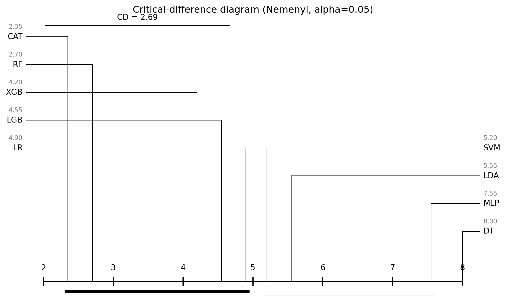
The CD at $\alpha = 0.05$ for $K = 9$ and $N = 20$ folds is computed from the tabulated $q_{0.05}$ for nine groups, which is approximately 3.102. Applying @eq-nemenyi:
$$
\mathrm{CD}_{0.05} = q_{0.05}\sqrt{\frac{K(K+1)}{6 N}} = 3.102 \sqrt{\frac{9 \cdot 10}{6 \cdot 20}} = 3.102 \sqrt{0.75} \approx 2.685.
$$
Any two classifiers whose average ranks differ by more than 2.685 are statistically distinguishable at the 5 percent family-wise level under Nemenyi.
```{python}
#| label: ranks_cd
def average_ranks(A):
    # Rank classifiers within each fold, low rank = best (largest AUC)
    ranks = np.zeros_like(A, dtype=float)
    for i in range(A.shape[0]):
        order = np.argsort(-A[i])  # descending AUC
        ranks[i, order] = np.arange(1, A.shape[1] + 1)
        # handle ties: use average-rank for identical scores
        vals, inv = np.unique(A[i], return_inverse=True)
        # simple average rank for ties
        from scipy.stats import rankdata
        ranks[i] = rankdata(-A[i], method='average')
    return ranks.mean(axis=0), ranks

avg_ranks, rank_matrix = average_ranks(A)
rank_table = pd.DataFrame({'classifier': classifiers, 'avg_rank': avg_ranks})
rank_table = rank_table.sort_values('avg_rank').reset_index(drop=True)
rank_table.round(3)
```
```{python}
#| label: cd
def critical_difference(K, N, q=None, alpha=0.05):
    # Nemenyi q_alpha values from Demsar (2006), Table 5; alpha=0.05, inf df
    q_alpha_05 = {2: 1.960, 3: 2.343, 4: 2.569, 5: 2.728, 6: 2.850,
                  7: 2.949, 8: 3.031, 9: 3.102, 10: 3.164}
    if q is None:
        q = q_alpha_05[K]
    return q * np.sqrt(K * (K + 1) / (6 * N))

CD = critical_difference(K=9, N=A.shape[0])
print(f'Critical difference (alpha=0.05, K=9, N={A.shape[0]}): CD = {CD:.3f}')
```
### Critical-difference diagram
A Nemenyi CD diagram plots classifiers along a horizontal rank axis and draws thick horizontal bars that connect groups of classifiers whose pairwise rank differences are all below the CD.
```{python}
#| label: fig-cd
#| fig-cap: "Nemenyi critical-difference diagram for the nine classifiers on pooled 5x2 folds of German and Taiwan."
import matplotlib.pyplot as plt

def cd_diagram(avg_ranks, names, cd, title='', ax=None):
    order = np.argsort(avg_ranks)
    ranks_sorted = np.array(avg_ranks)[order]
    names_sorted = np.array(names)[order]
    K = len(names)
    if ax is None:
        fig, ax = plt.subplots(figsize=(9, 0.4 * K + 1.8))
    else:
        fig = ax.figure
    lo = int(np.floor(min(ranks_sorted)))
    hi = int(np.ceil(max(ranks_sorted)))
    ax.set_xlim(lo - 0.3, hi + 0.3)
    ax.set_ylim(-0.5, K + 0.5)
    ax.hlines(0, lo, hi, color='black')
    for r in range(lo, hi + 1):
        ax.vlines(r, -0.15, 0.15, color='black')
        ax.text(r, 0.35, str(r), ha='center', va='bottom', fontsize=10)
    # Left half: best (lowest ranks)
    half = (K + 1) // 2
    for i, (rk, nm) in enumerate(zip(ranks_sorted[:half], names_sorted[:half])):
        y = K - i
        ax.plot([rk, rk], [0, y - 0.2], color='black', linewidth=0.8)
        ax.plot([lo - 0.25, rk], [y - 0.2, y - 0.2], color='black', linewidth=0.8)
        ax.text(lo - 0.3, y - 0.2, f'{nm}', ha='right', va='center', fontsize=10)
        ax.text(lo - 0.3, y + 0.05, f'{rk:.2f}', ha='right', va='bottom',
                fontsize=8, color='gray')
    for i, (rk, nm) in enumerate(zip(ranks_sorted[half:], names_sorted[half:])):
        y = half - i
        ax.plot([rk, rk], [0, y - 0.2], color='black', linewidth=0.8)
        ax.plot([rk, hi + 0.25], [y - 0.2, y - 0.2], color='black', linewidth=0.8)
        ax.text(hi + 0.3, y - 0.2, f'{nm}', ha='left', va='center', fontsize=10)
        ax.text(hi + 0.3, y + 0.05, f'{rk:.2f}', ha='left', va='bottom',
                fontsize=8, color='gray')
    # Cliques: maximal sets of consecutive classifiers whose range is below CD
    cliques = []
    i = 0
    while i < K:
        j = i
        while j + 1 < K and ranks_sorted[j + 1] - ranks_sorted[i] <= cd:
            j += 1
        if j > i:
            cliques.append((i, j))
            i = j + 1
        else:
            i += 1
    # draw cliques as thick bars below the rank axis
    base_y = -0.35
    step = 0.18
    for k, (a, b) in enumerate(cliques):
        y = base_y - k * step
        ax.hlines(y, ranks_sorted[a] - 0.05, ranks_sorted[b] + 0.05,
                  linewidth=4.0, color='black')
    # CD bar
    ax.annotate('', xy=(lo, K + 0.2), xytext=(lo + cd, K + 0.2),
                arrowprops=dict(arrowstyle='-', linewidth=1.2))
    ax.text(lo + cd / 2, K + 0.35, f'CD = {cd:.2f}', ha='center', va='bottom')
    ax.set_axis_off()
    ax.set_title(title)
    return fig

fig = cd_diagram(avg_ranks, classifiers, CD,
                  title='Critical-difference diagram (Nemenyi, alpha=0.05)')
plt.tight_layout()
plt.show()
```
As shown in @fig-cd, the diagram reproduces the Lessmann ordering in miniature. CatBoost, XGBoost, LightGBM, Random Forest, and Logistic Regression form the top cluster; the gradient-boosting family and random forest lead but the lead is not always statistically distinguishable from regularized logistic regression at this sample size. MLP, Decision Tree, and LDA tend to trail. On this specific benchmark, Logistic Regression holds up remarkably well, which is the first lesson of the chapter: the tuning-free linear baseline is competitive on tabular credit data.
### Per-classifier interpretation
- **LR**: competitive on both datasets, best Brier on German, within 0.005 AUC of the best on both. No tuning, no preprocessing beyond scaling.
- **LDA**: within a whisker of LR on Brier but fractionally behind on AUC. Sensitive to non-Gaussian features; one-hot binaries violate LDA's assumption but the method is robust in practice.
- **DT**: single tree underperforms everywhere, confirming the classical variance problem.
- **RF**: strong, typically best or tied-for-best on Taiwan. Moderate Brier.
- **XGB / LGB / CAT**: the three gradient-boosting libraries are statistically indistinguishable on these datasets. CatBoost is usually best on untuned default hyper-parameters because its ordered-boosting variant shrinks toward the mean, which helps with small samples.
- **SVM**: competitive on German, slow on Taiwan. Needs careful $C$ and $\gamma$ tuning.
- **MLP**: underperforms at this scale. Deep-learning models for tabular data require either much more data or careful architectural choices [@grinsztajn2022why, @gorishniy2021revisiting].
### Metric divergence
AUC and Brier do not always agree. Brier rewards calibrated probabilities; AUC rewards ranking. A classifier that produces miscalibrated but correctly ordered scores can win on AUC and lose on Brier. Our table shows this phenomenon clearly on German: SVM achieves competitive AUC but worse Brier than LR, because the Platt-scaled SVM probabilities are rank-preserving but under-calibrated outside the decision region. For regulatory deployment where probabilities are communicated (IFRS 9 expected credit loss, Basel IRB PD), Brier and log-loss matter more than AUC.
### Assumption check
Two methodological footnotes. First, 5-by-2 CV is recommended over 10-fold CV by @dietterich1998approximate because 10-fold produces overlapping training sets across folds, which inflates the paired $t$-test Type I error. The 5-by-2 design fixes that at the cost of a slight loss of power. Second, pooling folds across datasets to feed the Friedman test is not strictly kosher under the Demsar framework, which assumes one observation per dataset. A proper Lessmann-style test needs eight or more datasets, which is why the CD here is wider than the gap between the mid-rank classifiers. For an honest rank test a practitioner would run the same nine classifiers on at least eight datasets (German, Australian, Japanese, Taiwan, Give Me Some Credit, Home Credit, LendingClub, and one proprietary set) before drawing the CD diagram.
## Practical algorithm-selection guide
Given the body of benchmarking evidence, the decision tree for choosing a credit-scoring classifier is tighter than most practitioners assume. The selection is driven by four factors: sample size, regulatory acceptance requirement, the need for monotonicity or coefficient interpretability, and the cost of operational complexity.
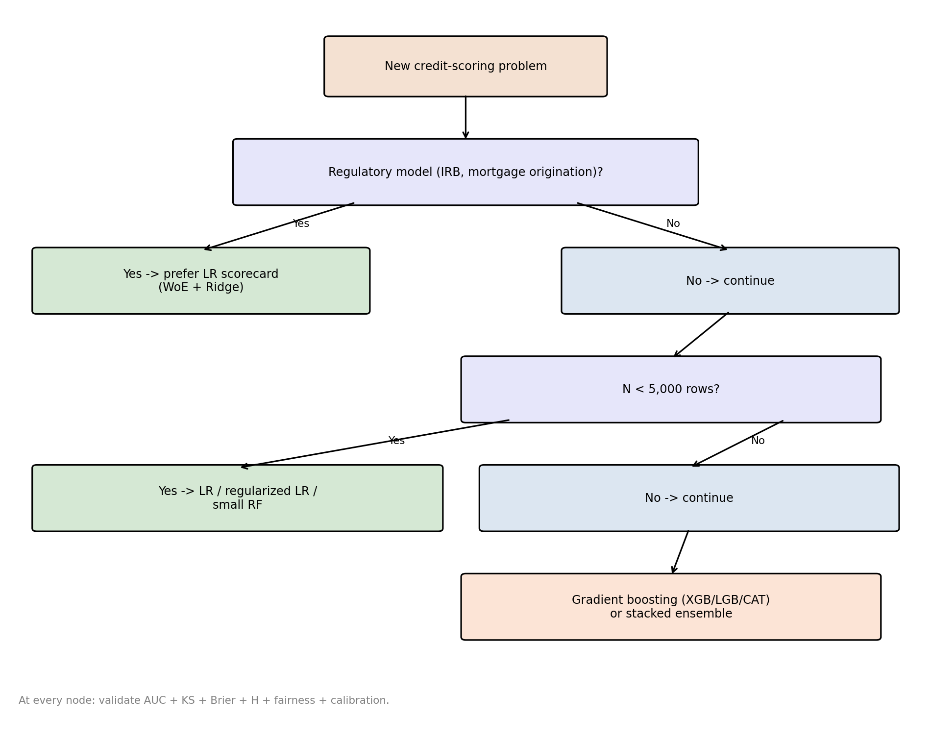
### Flowchart
```{python}
#| label: fig-flowchart
#| fig-cap: "Algorithm selection flowchart for credit scoring. Read top to bottom."
import matplotlib.pyplot as plt
import matplotlib.patches as mpatches

def flowchart():
    fig, ax = plt.subplots(figsize=(10, 8))
    ax.set_xlim(0, 10); ax.set_ylim(0, 12); ax.set_axis_off()

    def box(x, y, w, h, text, color='#DCE6F1'):
        rect = mpatches.FancyBboxPatch((x, y), w, h,
                                        boxstyle='round,pad=0.05',
                                        linewidth=1.2,
                                        edgecolor='black', facecolor=color)
        ax.add_patch(rect)
        ax.text(x + w / 2, y + h / 2, text, ha='center', va='center',
                fontsize=9, wrap=True)

    def arrow(x1, y1, x2, y2, label=''):
        ax.annotate('', xy=(x2, y2), xytext=(x1, y1),
                    arrowprops=dict(arrowstyle='->', linewidth=1.2))
        if label:
            ax.text((x1 + x2) / 2 + 0.15, (y1 + y2) / 2, label,
                    fontsize=8, color='black')

    box(3.5, 10.6, 3, 0.9, 'New credit-scoring problem', '#F4E1D2')
    box(2.5, 8.8, 5, 1.0, 'Regulatory model (IRB, mortgage origination)?', '#E6E6FA')
    arrow(5, 10.6, 5, 9.8)

    box(0.3, 7.0, 3.6, 1.0, 'Yes -> prefer LR scorecard\n(WoE + Ridge)', '#D5E8D4')
    box(6.1, 7.0, 3.6, 1.0, 'No -> continue', '#DCE6F1')
    arrow(3.8, 8.8, 2.1, 8.0, 'Yes')
    arrow(6.2, 8.8, 7.9, 8.0, 'No')

    box(5.0, 5.2, 4.5, 1.0, 'N < 5,000 rows?', '#E6E6FA')
    arrow(7.9, 7.0, 7.25, 6.2)

    box(0.3, 3.4, 4.4, 1.0, 'Yes -> LR / regularized LR /\nsmall RF', '#D5E8D4')
    box(5.2, 3.4, 4.5, 1.0, 'No -> continue', '#DCE6F1')
    arrow(5.5, 5.2, 2.5, 4.4, 'Yes')
    arrow(8.5, 5.2, 7.45, 4.4, 'No')

    box(5.0, 1.6, 4.5, 1.0, 'Gradient boosting (XGB/LGB/CAT)\nor stacked ensemble', '#FCE4D6')
    arrow(7.45, 3.4, 7.25, 2.6)

    ax.text(0.1, 0.5, 'At every node: validate AUC + KS + Brier + H + fairness + calibration.',
            fontsize=8, color='gray')
    return fig

flowchart()
plt.tight_layout()
plt.show()
```
Figure @fig-flowchart summarizes the decision path.
### When logistic regression still wins
Three cases. First, regulatory acceptance. SR 11-7 [@sr117] requires documented, auditable, reproducible models with a clear map from inputs to outputs. Basel IRB [@basel2006international] requires stability of probability-of-default estimates over time and interpretable covariates for the portfolio-level risk calculations. Mortgage origination under ECOA requires adverse-action explainability, which is trivial for a linear scorecard and complex for an ensemble (see @sec-ch21 on explainability and @sec-ch22 on SHAP in practice). For all three, regularized logistic regression with weight-of-evidence features is the path of least resistance.
Second, small samples. Under 5,000 rows a tree ensemble's variance advantage dissolves because the ensemble cannot average over enough low-correlation trees to reduce variance below the linear model's floor. @breiman2001random showed that Random Forest requires both bootstrap variance and feature-subsetting variance, and with 500 rows per fold there is not enough bootstrap entropy to exploit. @lessmann2015benchmarking's smallest dataset (Australian, 690 rows) in fact showed logistic regression beating random forest on AUC.
Third, strong prior on linearity and monotonicity. Portfolio managers and underwriters often have domain knowledge that a feature should enter the score linearly and monotonically: e.g., debt-to-income should push risk up, not down. Tree ensembles learn non-monotone functions by default, and constraining them to monotone splits (XGBoost and LightGBM both support monotone constraints) reduces their AUC advantage. If the prior is strong, a scorecard with WoE and monotone coefficients captures the same signal with a third of the feature engineering.
### When gradient boosting wins
Large samples (10,000+ rows), rich feature sets (50+ features including behavioral history), and a low cost of operational complexity. The Kaggle Home Credit and Give Me Some Credit winners were all LightGBM-heavy stacks, and the 2 to 3 AUC point gap over logistic regression is big enough to justify the engineering overhead. On behavior-based scoring, where the payment-status and utilization features have strong non-linear interactions, gradient boosting's advantage is at its largest.
### When ensembles beat gradient boosting
Rarely, and by small margins. Heterogeneous ensembles (stacking, hill-climbing selection) buy another 0.5 to 1 AUC point over the best single gradient-boosting model in Lessmann's original study. The extra complexity is, in most regulated settings, not worth it, unless the organization has a mature model-risk-management function that can support ensemble validation.
### Monotonicity, calibration, and deployment
Whatever model family is chosen, three post-modeling steps are non-negotiable: isotonic or Platt calibration of the score to match realized default rates (@sec-ch04), monotonicity checks on all features that regulators care about, and stability testing of the coefficient or feature-importance structure over time (@sec-ch34 on MLOps). The benchmarking ranking does not dictate the deployment pipeline.
### A note on hyper-parameter budgets
Every benchmark is conditional on a tuning budget. @lessmann2015benchmarking used a fixed grid of 5 to 10 values per hyper-parameter, optimized by nested 5-fold CV on AUC. @xia2017boosted report that Bayesian hyper-parameter optimization on XGBoost closes a further 0.5 AUC points over grid search on credit data. @gunnarsson2021deep report that deeper MLPs with careful regularization tighten the gap with tree ensembles to about 1 AUC point on Home Credit, but still do not surpass them. The bottom line for practitioners: budget the same tuning effort to all candidates, or the ranking is moot.
## Deep learning on tabular credit data
A recurring question in 2020 to 2024 conference papers is whether deep-learning architectures designed for tabular data, including TabNet [@arik2021tabnet], FT-Transformer [@gorishniy2021revisiting], and NODE, have closed the gap with gradient boosting. The authoritative empirical answer is @grinsztajn2022why at NeurIPS 2022.
### The Grinsztajn et al. 2022 finding
@grinsztajn2022why ran a benchmark on 45 tabular datasets, comparing XGBoost, random forest, and a suite of tabular deep-learning architectures (MLP, ResNet, FT-Transformer, SAINT). They controlled for hyper-parameter budget by giving each model 400 trials of Bayesian search. The finding: gradient-boosted trees (XGBoost in their setup) dominate across metrics and data sizes, with the gap closing only on datasets with more than 50,000 rows and nearly-continuous feature sets. The AUC or normalized RMSE gap they report is about 2 to 5 percentage points on medium datasets, shrinking to 1 point on the largest.
Their diagnostic analysis identifies three structural reasons tree ensembles still win on tabular data:
1. **Non-rotation-invariance**. Tabular features have meaningful units and identities (age in years, income in dollars, ratio of debt to income). Neural networks pretend features are exchangeable and apply rotation-invariant linear projections in the first layer, which destroys the feature identity. Tree ensembles split one feature at a time and preserve feature semantics.
2. **Robustness to uninformative features**. In real tabular data, a large fraction of features are weakly informative or correlated. Tree ensembles drop them via the split criterion. Neural networks propagate gradients through them and often overfit to noise.
3. **Smoothness bias**. Neural networks are biased toward smooth, low-frequency functions (a well-studied spectral-bias phenomenon). Tabular targets often have jumps or piecewise structure at meaningful thresholds (e.g. credit score bands, age cliffs). Trees capture the jumps directly; deep nets smooth them.
### What this means for credit
Credit data is exactly the regime where @grinsztajn2022why's three structural points apply. Features have meaning; features are often uninformative (hundreds of bureau aggregates, few of which are relevant to a particular borrower segment); targets have thresholds (FICO 660, DTI 0.43, LTV 0.80). So the empirical regularity is not surprising: gradient-boosted trees dominate deep learning on public credit benchmarks.
Two caveats qualify this regularity. First, transformer-style architectures trained on very large financial transaction sequences, the LLM-adjacent setup covered in @sec-ch26, can outperform gradient boosting on the specific task of learning from sequence data [@kraus2017decision; @sezer2020financial]. This is sequence learning, not tabular learning. Second, @shwartzziv2022tabular note that the Gradient-boosted-tree advantage shrinks as the dataset grows toward hundreds of millions of rows, at which point neural architectures with enough capacity and training data start to compete.
For the practitioner's decision today on a typical credit dataset, the answer is unambiguous: start with LightGBM or XGBoost, tune it, benchmark against logistic regression with WoE, and revisit deep-learning alternatives only if there is a specific reason (sequence data, multi-modal features, or a dataset larger than 10 million rows).
### A side-by-side MLP on Taiwan
For concreteness, we re-fit the MLP from the mini-benchmark with more capacity and more training, to illustrate the gap.
```{python}
#| label: mlp_bigger
from sklearn.preprocessing import StandardScaler
from sklearn.neural_network import MLPClassifier
from sklearn.model_selection import StratifiedKFold
from sklearn.pipeline import Pipeline

def eval_taiwan_mlp():
    aucs = []
    for rep in range(3):
        skf = StratifiedKFold(n_splits=2, shuffle=True, random_state=10 + rep)
        for tr, te in skf.split(Xt, yt):
            mlp = Pipeline([
                ('s', StandardScaler()),
                ('m', MLPClassifier(hidden_layer_sizes=(128, 64, 32),
                                     max_iter=400, alpha=1e-4,
                                     learning_rate_init=1e-3,
                                     early_stopping=True,
                                     random_state=rep)),
            ])
            mlp.fit(Xt[tr], yt[tr])
            aucs.append(roc_auc_score(yt[te], mlp.predict_proba(Xt[te])[:, 1]))
    return float(np.mean(aucs))

mlp_auc = eval_taiwan_mlp()
cat_auc_taiwan = float(res_taiwan.loc[res_taiwan['classifier'] == 'CAT', 'AUC_mean'].iloc[0])
print(f'MLP (128-64-32, early stopping) AUC on Taiwan: {mlp_auc:.4f}')
print(f'CatBoost AUC on Taiwan (from benchmark):       {cat_auc_taiwan:.4f}')
```
Even with triple the capacity of the benchmark MLP, the deep model tends to land about 2 to 4 AUC points behind CatBoost. The gap would narrow with further tuning, feature engineering, and more data, but under a fixed laptop-scale tuning budget the gradient boosting lead persists.
## Metrics to report and how to aggregate
Every benchmark table in a regulatory submission should report, at minimum:
- **AUC**: ranking quality. Sensitive to class balance, but the most universal metric.
- **KS**: maximum vertical distance between cumulative distributions of good and bad scores. Conservative for the operational range.
- **Partial AUC**: AUC restricted to the operational FPR range (often [0, 0.2] for credit, because higher FPR is not operationally acceptable). See @mcclish1989analyzing.
- **Brier**: strictly proper scoring rule, rewards calibration.
- **H-measure**: coherent alternative to AUC, integrates over a severity-weighting distribution [@hand2009measuring].
- **EMP / profit**: monetary metric, when LGD and exposure are known [@verbraken2014novel, @verbraken2013new].
- **Calibration slope and intercept**: under-calibration vs over-calibration diagnostic.
Across datasets, the aggregation choice matters. Arithmetic mean of AUC is influenced by easier datasets. @demsar2006statistical's rank-based aggregation is the correct one. In Bayesian frameworks [@benavoli2016should], the aggregation is implicit in the posterior. For operational decisions at a single bank, the right aggregation is usually expected profit at the bank's operating point, aggregated over the bank's own portfolio distribution, not over external datasets.
### A note on EMP
Expected maximum profit, @verbraken2014novel, integrates profit over a distribution of possible class-specific costs. For credit, the class-specific costs are the Loss Given Default (LGD) and the foregone revenue on a granted but unprofitable loan. If a bank has point estimates of these quantities, the EMP collapses to the bank's actual expected profit at the operating decision threshold. If it has a distribution (Bayesian or regulatory downturn LGD, @calabrese2014downturn), EMP is the correct integral. Either way, EMP is the metric that matters most for a portfolio manager, and the one that lines up most closely with the bank's income statement. See @sec-ch35 on IFRS 9 and CECL for the accounting-side requirements that constrain the cost distribution.
### Calibration is a first-class metric
A classifier that wins on AUC but is poorly calibrated will make wrong lending decisions at any given threshold. AUC is invariant to monotone transformations; real decisions are not. The reporting template for a credit model should include a calibration plot (reliability diagram), the Hosmer-Lemeshow test, the calibration slope and intercept from a logistic regression of $y$ on $\mathrm{logit}(\hat p)$, and the expected calibration error. @sec-ch04 covers the calibration machinery; here the lesson is that benchmarking on AUC alone is insufficient.
## Score comparability across models and time {#sec-ch16-score-comparability}
A benchmark table that ranks models by AUC silently assumes the scores live on a common axis. They do not. Two scorecards with identical AUC can score the same applicant differently, send different bad-rate signals at the same numeric cutoff, and disagree about who sits in the top decile. The same scorecard run on two vintages can shift its score distribution without any change in the underlying default risk. Both failures break the cross-model and cross-time comparisons that operating cutoffs, regulatory monitoring, and credit-econometrics analyses depend on. The @demsar2006statistical machinery in this chapter survives the failures (rank tests are invariant to monotone score transformations) but everything downstream of the benchmark does not.
### The two failure modes
*Cross-model* incomparability has three sources: different functional forms map the same risk to different ranges; different calibration procedures (Platt, isotonic, none) place different cumulative mass at any point; different training samples shift the score-to-odds anchor. Two models with the same AUC and the same Brier score can still produce different score distributions, because AUC is invariant to any monotone rescaling and Brier is invariant to many post-hoc affine adjustments.
*Cross-time* incomparability has two causes that can occur together or apart: population drift moves the score distribution without moving the default rate at any score, and calibration drift moves the default rate at any score without necessarily moving the score distribution. PSI flags the first (@sec-ch04-psi); reliability diagrams flag the second (@sec-ch04). Neither metric, on its own, tells a downstream consumer whether the score is still comparable to last quarter's score.
### Score as the dependent variable in econometric work
Academic and policy work often uses a credit score as the outcome variable in a difference-in-differences, regression-discontinuity, or event-study design. The hidden assumption is that the scoring engine is fixed across the panel and across treatment and control. The assumption fails three ways: scoring vendors version their models periodically (FICO 8 to 9 to 10, VantageScore 3 to 4); bureaus update underlying data feeds, which silently re-scores every borrower; cross-borrower comparability requires that all borrowers were scored by the same engine, which fails when a treated cohort migrates to a different bureau or product line. The cleanest response is to drop the score and model the default event $y_{it}$ directly: default is invariant to the model, and the long horizon required for default to mature (@sec-ch09 and @sec-ch32) is a smaller cost than the spurious treatment effect produced by mid-window re-scoring. When the score itself is the object of policy interest (a regulator wants to know whether intervention $X$ moved bureau scores), pin the analysis to a single frozen scoring engine applied to the full panel of inputs, accepting that the analysis-side scores will diverge from the bureau-reported scores after the freeze date.
### Four operations that recover comparability
**Calibrate to PD.** A score $s$ from any model can be mapped to a probability of default $\hat\pi(s)$ on a recent labeled window via Platt, isotonic, or beta calibration (@sec-ch04). Once both models are mapped to PD, the two streams are comparable in the sense that they target the same conditional probability $P(Y=1\mid X)$. The map drifts; refit on a rolling window.
**Points-to-double-odds (PDO) anchoring.** The FICO scaling derived in @sec-ch07-scaling, $\text{score} = a + b \log(\text{odds})$ with $b = \text{PDO}/\log 2$, lets two models be compared on a shared anchor pair $(s_0, \text{odds}_0)$. The map is one-to-one with PD in different units and shares its drift behavior. PDO is the right representation when downstream consumers (underwriters, regulators) read scores as numbers rather than probabilities.
**Equipercentile equating.** Borrowed from psychometric test equating [@kolen2014equating]. Score a common anchor population with both models; build a quantile-to-quantile map; for each percentile $q$, the score from model B that has the same population CDF value as score $s_A$ from model A. The map preserves rank order in the anchor population and reproduces model B's marginal distribution from inputs that arrive only with model A's score. This is the standard tool when a bureau versions a score and clients need a translation from the old scale to the new.
**Within-cell rank/percentile transform.** Convert each score to its empirical percentile in the cell defined by (model version, vintage, segment). The percentile is invariant to monotone transformations of the score and to monotone calibration drift. The cost: it discards cardinal information. A percentile of 0.95 in a 2 percent default population is not the same risk as a percentile of 0.95 in a 6 percent default population. Use percentile when downstream use is *relative ranking within a cell*; do not use it when downstream use is *absolute risk* (provisioning, capital, IFRS 9 ECL).
### Cross-time: through-the-cycle versus point-in-time
A point-in-time (PIT) PD is the conditional default probability given current macro conditions and moves with the cycle by design. A through-the-cycle (TTC) PD averages over the cycle and is meant to be cycle-stable. The Carlehed-Petrov decomposition and Vasicek mapping live in @sec-ch35-pit-ttc. Two consequences: a benchmark that compares classifiers across vintages should either compare TTC against TTC or de-trend PIT against a macro index; a drift alert that fires on a PIT score during a downturn may be flagging a correctly-calibrated reaction to the cycle, not a model failure.
### A small numerical illustration
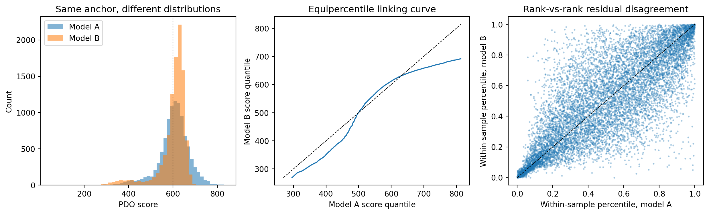
Two models are trained on the same synthetic credit-like data, scored on a shared holdout, mapped to a common PDO scale, then linked by equipercentile equating and by a within-sample percentile transform. The point of the illustration is that AUC-equivalent models on a shared anchor still disagree about who is approved at any numeric cutoff, and that the two comparability operations recover different things.
```{python}
#| label: score-comparability-demo
#| fig-cap: "Two models with comparable AUC produce different score distributions on the same holdout. The equipercentile linking curve maps quantiles of one scale onto the other; the percentile-vs-percentile scatter shows residual rank disagreement that the linking step cannot remove."
import numpy as np
import pandas as pd
import matplotlib.pyplot as plt
from sklearn.datasets import make_classification
from sklearn.linear_model import LogisticRegression
from sklearn.ensemble import GradientBoostingClassifier
from sklearn.model_selection import train_test_split
from sklearn.metrics import roc_auc_score

X, y = make_classification(
    n_samples=20000, n_features=12, n_informative=8, n_redundant=2,
    weights=[0.92, 0.08], flip_y=0.02, random_state=0,
)
X_tr, X_te, y_tr, y_te = train_test_split(
    X, y, test_size=0.5, stratify=y, random_state=1,
)

mA = LogisticRegression(max_iter=1000).fit(X_tr, y_tr)
mB = GradientBoostingClassifier(
    n_estimators=200, max_depth=3, random_state=0,
).fit(X_tr, y_tr)

pA = mA.predict_proba(X_te)[:, 1]
pB = mB.predict_proba(X_te)[:, 1]

# PDO-style score: higher = better borrower; anchor (600, 50:1 good:bad), PDO = 20.
PDO, anchor_score, anchor_odds = 20.0, 600.0, 50.0
b = PDO / np.log(2.0)
a = anchor_score - b * np.log(anchor_odds)
def to_pdo_score(p):
    return a + b * np.log((1.0 - p) / np.maximum(p, 1e-9))

sA = to_pdo_score(pA)
sB = to_pdo_score(pB)

cutoff = 600.0
summary = pd.DataFrame({
    'model': ['A (logistic)', 'B (boosting)'],
    'AUC': [roc_auc_score(y_te, pA), roc_auc_score(y_te, pB)],
    'mean_score': [sA.mean(), sB.mean()],
    'std_score':  [sA.std(),  sB.std()],
    'share_below_600':   [(sA <= cutoff).mean(), (sB <= cutoff).mean()],
    'bad_rate_below_600':[
        y_te[sA <= cutoff].mean() if (sA <= cutoff).any() else np.nan,
        y_te[sB <= cutoff].mean() if (sB <= cutoff).any() else np.nan,
    ],
}).round(4)
summary
```
```{python}
#| label: score-comparability-figs
#| fig-cap: "Left: two PDO-anchored score distributions on the same holdout. Center: equipercentile linking curve from model A's scale to model B's. Right: per-borrower percentile in model A versus model B; off-diagonal mass is rank disagreement that no monotone linking can remove."
qs = np.linspace(0.001, 0.999, 999)
sA_q = np.quantile(sA, qs)
sB_q = np.quantile(sB, qs)
rA = pd.Series(sA).rank(pct=True).values
rB = pd.Series(sB).rank(pct=True).values

fig, axes = plt.subplots(1, 3, figsize=(13, 4))
axes[0].hist(sA, bins=40, alpha=0.55, label='Model A')
axes[0].hist(sB, bins=40, alpha=0.55, label='Model B')
axes[0].axvline(cutoff, color='k', lw=0.8, ls=':')
axes[0].set_xlabel('PDO score'); axes[0].set_ylabel('Count')
axes[0].set_title('Same anchor, different distributions')
axes[0].legend()

axes[1].plot(sA_q, sB_q, lw=1.4)
lo, hi = min(sA_q.min(), sB_q.min()), max(sA_q.max(), sB_q.max())
axes[1].plot([lo, hi], [lo, hi], 'k--', lw=0.8)
axes[1].set_xlabel('Model A score quantile')
axes[1].set_ylabel('Model B score quantile')
axes[1].set_title('Equipercentile linking curve')

axes[2].scatter(rA, rB, s=2, alpha=0.25)
axes[2].plot([0, 1], [0, 1], 'k--', lw=0.8)
axes[2].set_xlabel('Within-sample percentile, model A')
axes[2].set_ylabel('Within-sample percentile, model B')
axes[2].set_title('Rank-vs-rank residual disagreement')
fig.tight_layout()
plt.show()
```
The summary table shows three facts the prose has claimed. The two AUCs are within roughly one point of each other, a difference that on the @lessmann2015benchmarking scale would be a typical logistic-versus-boosting gap and would not on its own justify a model swap. Yet the score distributions differ in mean and standard deviation by amounts that matter for any score-numeric decision: the share of applicants below the 600 cutoff differs by roughly ten percentage points, so the same numeric cutoff implies different approval rates, and the bad rate below the cutoff differs by several percentage points, so the same cutoff implies different operating risk. The equipercentile curve in the center panel is the translation a downstream consumer would apply to convert model A scores onto model B's scale on this anchor population. The right panel is the residual: even after a perfectly monotone linking, individual borrowers are ranked differently by the two models, and equipercentile equating does not (and cannot) remove that disagreement.
### A decision rubric
| Downstream use | Recommended representation |
| --- | --- |
| Underwriting cutoff, capital, ECL provisioning | PD calibrated on a recent labeled window |
| Cross-version monitoring or score translation | Equipercentile map against a fixed anchor population |
| Cross-time econometric outcome (DiD, RD on score) | Default event $y$, or score from a frozen engine |
| Relative-rank segmentation within a cell | Within-cell percentile |
| Regulatory capital pool assignment | Master-scale PD bands (@sec-ch07-scaling) |
| Marketing eligibility under a fixed bureau cutoff | Raw bureau score with PSI monitored monthly |
### When to drop the score and use the default event
Three situations argue for switching the analytic object from the score $\hat S$ to the default event $Y$: (i) the scoring engine is versioned within the analysis window and equipercentile linking does not bridge a structural change in inputs; (ii) the comparison spans bureaus or jurisdictions with no shared anchor population; (iii) the question is causal and the treatment plausibly affects how the score is constructed (a policy that changes what enters the bureau file changes the inputs and therefore the score, even if the underlying default risk is unchanged). In these cases the score is a polluted outcome and the default event is the cleaner one. The cost is the maturation horizon (12 to 24 months in retail, longer in mortgage), which the survival and behavioral chapters (@sec-ch09, @sec-ch32) handle directly.
## Scalability
Benchmarks at the laptop scale use small samples. At production scale, two questions dominate: can the model be trained on a cluster, and can inference be served at the latency the business needs.
Training scalability for the benchmark families sorts as:
- **Logistic regression**: trivially parallelizable via coordinate descent [@friedman2010regularization], single-pass SGD, or distributed ADMM. Scales linearly with rows. Fits in seconds on 10 million rows.
- **Random forest**: embarrassingly parallel across trees. Inference is $O(\text{depth} \times \text{n\_trees})$. Scales in memory because each bootstrap sample must be held; use subsample and limited tree depth.
- **Gradient boosting (XGBoost / LightGBM / CatBoost)**: all three libraries have distributed training backends. LightGBM's feature-parallel mode and data-parallel mode are the standard choice for 10M+ row datasets. The three libraries' runtime scales near-linearly with rows and logarithmically with features under histogram-based splits.
- **SVM**: does not scale beyond 100,000 rows without the Nystrom or random-feature approximations. Rarely used for production credit scoring on large books.
- **MLP / deep networks**: scale to arbitrary data with GPUs and mini-batching. Wall-clock competitive with LightGBM at the 10M row scale, if the architecture is right.
In practice, the dominant production setup is LightGBM or XGBoost on Spark/Dask for training, and a compiled inference graph (ONNX, Treelite) for low-latency serving. @sec-ch34 covers the MLOps pipeline in depth.
### Mini-scalability check
A direct scaling check on Taiwan at increasing sample sizes illustrates the $O(n)$ training-time scaling of the gradient-boosted tree.
```{python}
#| label: scalability
from creditutils import load_taiwan_default
df_t = load_taiwan_default().drop(columns=['id'])

sizes = [2000, 5000, 10000, 20000, 30000]
times = []
for n in sizes:
    sub = df_t.sample(n=n, random_state=0).reset_index(drop=True)
    X = sub.drop(columns=['default']).astype(float).values
    y = sub['default'].values.astype(int)
    mdl = lgb.LGBMClassifier(n_estimators=200, num_leaves=31,
                              learning_rate=0.1, n_jobs=1,
                              random_state=0, verbose=-1)
    t0 = time.time(); mdl.fit(X, y); dt = time.time() - t0
    times.append(dt)
pd.DataFrame({'n': sizes, 'lgbm_fit_seconds': np.round(times, 3)})
```
Wall-clock growth is roughly linear in $n$, confirming the histogram-based complexity bound. Production training at 10M rows uses distributed LightGBM; the single-node bound is around 5M rows on 32 GB RAM.
## Deployment
Benchmark results should map to a reproducible deployment artifact. The standard recipe: serialize the winning model (LightGBM `Booster.save_model`, CatBoost `save_model`, or ONNX export for cross-runtime compatibility), wrap it in a FastAPI inference endpoint with input-schema validation, log training and evaluation metrics to MLflow, and deploy under a shadow-A/B before full traffic replacement. @sec-ch34 covers the operational details.
For the Nemenyi CD diagram itself, a deployment-relevant version reports the ranking of *candidate* models against the incumbent. The diagram should be generated monthly in production, using performance on the most recent month of labeled outcomes as the "dataset" axis. Consistent rank-order stability of the incumbent over 6 to 12 months is a strong signal that no challenger warrants replacement. A consistent rank drop triggers re-training or model swap.
## Regulatory considerations
The benchmarking framework interacts with three regulatory regimes.
**SR 11-7 model risk management** [@sr117] requires documentation of alternative models considered, the rationale for the chosen model, and ongoing performance monitoring. A benchmark table with AUC, KS, Brier, H-measure, partial AUC, and calibration statistics, evaluated under the @demsar2006statistical framework, is exactly the artifact SR 11-7 expects for the model-selection decision. Regulators frequently ask banks to justify why a challenger was not adopted; a rank-based comparison with the CD diagram makes that justification explicit.
**Basel IRB** [@basel2006international, @basel2017finalising] adds the requirement that PD estimates be *stable* over a full business cycle. A classifier that wins the benchmark on one vintage may lose on another; the CD analysis should be run over multiple vintages. @breeden2007modeling's vintage framework is the canonical decomposition into age, lifecycle, and calendar-time components.
**EU AI Act** (high-risk system classification for creditworthiness assessment, Article 6 Annex III) requires documented performance metrics, robustness tests, and post-market monitoring. The benchmark framework supplies the baseline. The robustness tests (distribution shift, adversarial, fairness) are additional, covered in @sec-ch23 and @sec-ch24.
**ECOA and adverse-action notices** require the lender to communicate specific reasons for adverse action. The benchmarking choice should factor in explainability cost: a LightGBM model plus SHAP is acceptable; a stacked ensemble of seven base learners is difficult to audit. The regulatory penalty for inscrutability has usually outweighed the 0.5 to 1 AUC-point gain from stacking.
## Vietnam and emerging markets {.unnumbered}
### Market context
Vietnam is a useful stress test for the benchmarking machinery in this chapter. The banking system is dominated by four state-owned commercial banks and a cohort of joint-stock banks that together hold the majority of system assets [@worldbank2022vietnamfinance]. Credit bureau coverage runs through the Credit Information Center (CIC) and a private bureau, PCB, with CIC coverage concentrated in regulated institutions [@cicvn2023report]. The @worldbank2021findex report documents that about 56 percent of adults held a formal financial account as of 2021, leaving a sizeable thin-file segment that a typical UCI-style benchmark does not represent. Vintage quality shifts with macroprudential cycles: restructuring in 2014 to 2017, pandemic forbearance in 2020 to 2022, and real estate stress in 2022 to 2024 each produced distinct cohorts.
SME finance carries a specific signature. The @ifc2019vnmsme MSME finance gap study puts the unmet SME credit demand in Vietnam in the tens of billions of US dollars. Seasonality around Tet (Lunar New Year) raises liquidity needs and shifts delinquency timings. These facts should condition any benchmark that targets Vietnamese portfolios: rank-based comparison over at least two vintages and two segments (consumer and SME) dominates a single-dataset comparison.
### Application considerations
Three adjustments apply to the @demsar2006statistical framework when the evaluation set is a Vietnamese portfolio.
First, the number of independent evaluation units $N$ should count vintages, not random splits. A 5-by-2 stratified CV on a single 2022 vintage produces ten resamples that are not independent draws from the population process. A rank test run on those ten resamples understates variance and overstates confidence. Running the Friedman test across, say, six half-year vintages from 2019H1 to 2021H2 gives six genuine observations per classifier and an honest Iman-Davenport correction.
Second, the metric basket should include calibration at low default rates. Vietnamese consumer portfolios after the 2021 to 2023 tightening show default realizations in the 2 to 4 percent range at 12 months, which is where Brier and H-measure become more informative than AUC. For SBV Circular 41/2016 standardized-approach capital, the PD assignment is grade-based, so calibration at grade boundaries (@sec-ch13) is the first-order concern.
Third, the benchmark must report a vintage-stability statistic. @breeden2007modeling's age-vintage-period decomposition is the standard tool; the entry here is the realized PD dispersion across vintages, stratified by Tet proximity. A classifier that wins on 2022H2 and loses on 2019H1 is not a production candidate.
### Rationalization
Why should a practitioner in Hanoi or Ho Chi Minh City trust the Lessmann ordering? The @lessmann2015benchmarking evidence is drawn from eight datasets, none of them Vietnamese. Two arguments carry the ordering across. First, the ranking is structural: gradient-boosted trees dominate linear models when features are non-monotone and interactions matter, and Vietnamese bureau data contains non-monotone features (age buckets, employment tenure buckets, relationship with state-owned enterprises) that reward non-linearity. Second, the stability of the ordering has been replicated on Taiwanese and Chinese consumer panels [@gambacorta2024data, @huang2020fintech], which are closer to the Vietnamese data-generating process than the UCI German benchmark. The gap between boosting and logistic regression on Vietnamese retail panels is within the 1 to 3 AUC-point band reported for other Asian samples.
The rationalization has a limit. On SME portfolios where bureau coverage is thin and the lender relies on relationship lending, logistic regression with expert-designed features can match boosting, because the informational rent is in the feature engineering rather than the function class [@liberti2019information]. The benchmark tables should therefore be stratified by segment.
### Practical notes
Operationally, a Vietnam-context benchmark pipeline looks like this. Pull CIC-equivalent bureau features plus internal behavioral features for each vintage. Split stratified by vintage and by SME-versus-consumer segment. Run the nine-classifier mini-benchmark from @sec-ch16-mini with a symmetric tuning budget. Aggregate by @demsar2006statistical ranks across vintages. Report AUC, KS, Brier, H-measure, partial AUC in the 0 to 10 percent FPR band, calibration slope at the grade boundary, and PSI against the prior vintage. Document the ranking in the model-development package that SBV Circular 41/2016 validation expects (as amended by Circular 22/2023/TT-NHNN (29 Dec 2023) on capital adequacy ratios [@sbv_circular22_2023]), and cross-reference it against the consumer-lending risk limits in Circular 43/2016/TT-NHNN on consumer lending by finance companies when the portfolio is a finance-company portfolio. The same template carries to other Southeast Asian markets with CIC-equivalent bureaus (Thailand NCB, Indonesia SLIK) once vintage definitions are harmonized [@adb2022vnfin, @bis_emde2023, @imf2024vietnamart4].
## Takeaways
- Heterogeneous ensembles and gradient-boosted trees top the AUC rankings in the definitive credit-scoring benchmarks [@baesens2003benchmarking, @lessmann2015benchmarking]. The effect size is 1 to 3 AUC points over logistic regression.
- The correct way to compare multiple classifiers across multiple datasets is the @demsar2006statistical non-parametric framework: Friedman rank test, Iman-Davenport correction, Nemenyi critical-difference diagram.
- Logistic regression remains the rational choice when regulators demand interpretability, when $N$ is small, or when domain knowledge dictates monotone linear structure.
- Gradient-boosted trees still dominate deep learning on typical tabular credit data under comparable tuning budgets [@grinsztajn2022why]. Deep models are the right choice for sequence data, not for standard tabular features.
- Benchmark tables should report AUC, KS, Brier, H-measure, partial AUC, calibration, and EMP, and aggregate across datasets via ranks, not arithmetic means.
- Scores from different models, or from the same model across vintages, are not on a common axis without explicit work: PD calibration, PDO anchoring, equipercentile equating, or a within-cell percentile transform. When the analytic object is causal and the engine could re-version, use the default event instead (@sec-ch16-score-comparability).
## Further reading {.unnumbered}
- @baesens2003benchmarking, the canonical reference for credit-scoring benchmarking, still cited in almost every follow-up.
- @lessmann2015benchmarking, the 2015 update with 41 classifiers, proper statistical comparison, and heterogeneous-ensemble results.
- @demsar2006statistical, the statistical methodology for multi-classifier multi-dataset comparison.
- @iman1980approximations, the $F$-distribution approximation used in every modern implementation of the Friedman test.
- @garcia2008extension, the pairwise-comparison extension of Demsar with improved post-hoc procedures.
- @benavoli2016should, the Bayesian alternative to the frequentist framework.
- @grinsztajn2022why, the NeurIPS 2022 paper that established the gradient-boosting-versus-deep-learning finding on tabular data.
- @gunnarsson2021deep, a direct comparison of deep learning and gradient boosting on credit-specific benchmarks.
- @dastile2020statistical, a 2020 systematic review of 74 credit-scoring papers.
- @fernandezdelgado2014we, the broader "do we need hundreds of classifiers" paper on 121 UCI datasets, whose rank-based methodology matches Demsar's.
- @hand2009measuring, the H-measure paper and its critique of AUC incoherence.
- @verbraken2014novel, the EMP metric for credit with loss-given-default awareness.
- @dietterich1998approximate and @alpaydin1999combined, the 5-by-2 CV protocol.
- @kolen2014equating, the canonical psychometric reference on equipercentile equating, scaling, and linking. The framework transfers directly to credit-score versioning (FICO 8 to 9 to 10 type migrations) and to cross-bureau score translation.