---
execute:
echo: true
eval: true
---
# BigTech Credit and Non-Traditional Lenders {#sec-ch20}
::: {.callout-note appearance="simple" icon="false"}
**Scope: both retail and corporate.** BigTech lending stacks: consumer payment-history scoring (Alipay, WeChat) on the retail side and merchant or SME working-capital lending (MyBank, Ant) on the corporate side.
:::
## Overview {.unnumbered}
A platform that settles payments, ships packages, runs a chat app, or operates a marketplace knows things a bank cannot see. It knows the intraday velocity of a merchant's sales, the sentiment of buyer reviews, the stability of the supplier network, and the way a shopkeeper responds when a counterparty delays a shipment by three days. Traditional bureaus see a sliver of this reality, compressed into payment history and utilization ratios that lag by thirty to ninety days. BigTech lenders sit on the live stream.
This chapter studies what changes when a payment or commerce platform decides to underwrite. The empirical anchor is the Chinese fintech ecosystem, where Ant Financial (now Ant Group), WeBank, and MYbank built loan books running into the hundreds of billions of renminbi on top of Alipay and WeChat Pay data. The theoretical anchor is the data-versus-collateral trade-off studied by @gambacorta2024data and @bis2020data. We will formalize it, implement it, and break it with a carefully constructed simulation in which ML with platform data substitutes for a pledge of real estate.
The chapter treats six questions. How do BigTech lenders work, concretely, at the product level? What signal do they actually extract that bureaus miss? When does the platform-only posterior dominate a hybrid of bureau plus platform? How does collateral quality interact with the marginal value of alternative data? What does shadow banking look like when the shadow is a super-app? And what do platform feedback loops imply for antitrust, regulatory arbitrage, and the long-run distribution of credit?
### Notation {.unnumbered}
Let $Y \in \{0, 1\}$ denote default one year forward, $X^B$ denote bureau features, $X^P$ denote platform features (transactional, behavioral, operational), and $C$ denote pledgeable collateral with recovery rate $\rho \in [0, 1]$. PD denotes probability of default $p(Y = 1 \mid X)$, LGD denotes loss given default, $r$ the contract rate, and $r_f$ the funding rate. Bayesian model averaging posteriors are written $p(Y \mid X, \mathcal{M})$ with model space $\mathcal{M} = \{M_B, M_P, M_H\}$ for bureau-only, platform-only, and hybrid.
---
## Motivation {.unnumbered}
BigTech credit is an industrial-organization story that happens to run on machine learning. A payments app like Alipay processes billions of transactions per month. Every transaction produces structured features: amount, merchant category, timestamp, counterparty, device fingerprint, and settlement lag. Overlay chat data, logistics data, and marketplace data, and you have something that a bureau cannot replicate by aggregating monthly statements. The central empirical finding of @gambacorta2024data, @bis2020data, @frost2019bigtech, and @huang2020fintech is that this stream of data substitutes for the things that small borrowers lack: credit history, reliable financial statements, and real estate collateral.
The policy question is whether BigTech credit expands the frontier or merely shifts it. @buchak2018fintech show that U.S. fintech mortgage lenders grew partly through technology and partly through regulatory arbitrage; they can lend where banks cannot because capital requirements differ. @philippon2016fintech argues that the cost of financial intermediation has not fallen much despite technological change, and that fintech's biggest contribution may be in redistributing rents rather than shrinking them. @stulz2019fintech makes the opposite bet for BigTech: when a platform already holds payments data, the marginal cost of credit assessment is close to zero, and incumbency in commerce becomes incumbency in finance.
The statistical question is whether platform data dominates bureau data conditional on a given sample. The answer is conditional. For thin-file borrowers with no bureau history, the platform posterior strictly dominates because the bureau prior is uninformative. For thick-file borrowers, the hybrid posterior dominates because the two signal spaces are not redundant. @sec-ch20-gambacorta formalizes the condition.
The engineering question is how to build it. A BigTech underwriter cannot wait four weeks for a monthly statement feed. Decisions are made in seconds, at the moment of checkout or working capital request. The system must handle real-time feature stores, online XGBoost inference, and drift monitoring at second granularity. @sec-ch20 and @sec-ch20-platform discuss the design implications.
Vietnam deserves its own BigTech frame. MoMo, ZaloPay, VNPay, and Shopee Pay each operate consumer-scale payment stacks with tens of millions of actives, and all four are moving credit products to market either directly or through bank partnerships. The Vietnam-and-EM section at the end of this chapter reads these platforms next to Ant, WeBank, and Mercado Libre and asks what the @gambacorta2024data data-versus-collateral ordering implies for a Vietnamese policy designer.
## BigTech lender ecosystem {#sec-ch20-bigtech}
BigTech credit is a loose label. It covers firms whose primary business is not finance, but who extend credit on the back of a data-rich primary business. The canonical taxonomy, due to @frost2019bigtech and @cornelli2023fintech, distinguishes four archetypes: super-apps with embedded payment rails (Ant, Tencent, Kakao), e-commerce platforms with working capital arms (Amazon, Mercado Libre, Rakuten, Shopify), social platforms that monetize commerce (Line, Grab), and telecoms that originated mobile money (Safaricom M-Shwari, MTN MoMo). Each has a distinct data moat and a distinct regulatory envelope.
### Ant Group and the Alipay stack
Ant Group began as Alipay, the escrow layer for Taobao transactions in 2004. By 2020, Alipay processed more than ten trillion yuan in annual payment volume across more than a billion users. The credit arm, branched as Huabei (consumer BNPL), Jiebei (consumer cash loan), and MYbank (SME), issued roughly 1.7 trillion yuan of loans outstanding at peak. The loan products were originated through machine learning scorecards fed by the Alipay transaction graph, Sesame Credit behavioral tags, and merchant operations data from Taobao and Tmall.
Three design choices distinguish Ant from a retail bank. First, underwriting is stateless at the user level: a user's Huabei limit is recomputed nightly on the basis of transaction stream features, not underwritten once at application. Second, origination is channelless: there is no branch, no agent, and no application form. Third, capital is partially externalized through asset-backed securitization and bank partnerships, which became the focus of the 2020 regulatory crackdown by the People's Bank of China and the CBIRC.
Huabei is a consumption credit line, usually between a few hundred and a few thousand yuan, amortized over one to twelve months with a first month grace period. Jiebei is a cash credit line up to about three hundred thousand yuan. MYbank targets small merchants: its 3-1-0 product (three minutes to apply, one second to decide, zero human contact) was rolled out in 2015 and remains the reference design for BigTech SME lending globally [@frost2019bigtech; @huang2020fintech].
### Tencent and WeBank
Tencent's credit stack runs on WeChat and QQ rather than Alipay. WeBank, in which Tencent is the largest shareholder, launched Weilidai in 2015 as a consumer cash loan product distributed inside WeChat. Average ticket is about eight thousand yuan, and underwriting uses behavioral features from the chat app, payment graph, and social graph [@cornelli2023fintech]. WeBank's claim, corroborated by third-party analysis, is that its unit cost per loan decision is on the order of a few yuan, which is orders of magnitude below the hundreds of yuan spent by a state-owned bank on an equivalent SME decision.
### Amazon Lending and Shopify Capital
Amazon Lending and Shopify Capital are e-commerce-anchored BigTech lenders. Both target merchants on their respective platforms. Amazon Lending originates working capital advances of up to a few hundred thousand dollars, repaid as a fixed percentage of future sales routed through Amazon. Shopify Capital operates similarly. The underwriting features are almost entirely operational: gross merchandise volume, refund ratio, review volatility, inventory turnover, shipping performance, and catalog stability. Bureau features enter as negative gates (active bankruptcy, tax lien) but not as a primary signal.
The product design exploits a structural feature of platform lending: the lender controls the collection channel. A Shopify merchant repays through the Shopify checkout. A Taobao merchant repays through Alipay settlement. This eliminates the largest operational friction in SME lending, which is getting paid, and transfers part of the credit risk from the lender to the platform's willingness to keep the merchant onboarded.
### Mercado Libre, Rakuten, Kakao
Mercado Libre operates Mercado Credito in Argentina, Brazil, and Mexico. The model mirrors Amazon Lending but layers a payments rail (Mercado Pago) that reaches beyond the platform. This extends the credit base from pure marketplace merchants to offline merchants who accept Mercado Pago. The default risk on the offline pool is meaningfully higher, and Mercado Credito has historically priced this gap with risk-based pricing rather than rationing.
Rakuten's playbook is different: it is a financial conglomerate as much as it is a commerce platform. Rakuten Bank, Rakuten Card, and Rakuten Securities operate with an explicit loyalty-program cross-subsidy. Credit decisions are informed by Rakuten Super Points balances and e-commerce purchase patterns. The model is closer to a Japanese keiretsu than to a pure BigTech play.
Kakao built KakaoBank on top of KakaoTalk, the dominant chat app in South Korea. Its credit features are a blend of messaging behavior, peer transfer patterns, and mobile carrier payment history. KakaoBank reached profitability faster than any comparable digital bank in Asia, partly because customer acquisition cost inside KakaoTalk is close to zero [@cornelli2023fintech].
### Business model taxonomy
Three business model features distinguish BigTech lenders from bank lenders. First, distribution is zero marginal cost: the lender is already inside the user's primary app. Second, funding can be either deposit-funded (when a banking license exists), securitization-funded (Ant's ABS program), or balance-sheet funded off parent equity. Third, data is proprietary and non-portable: a bureau score is designed to be portable across lenders, while a Sesame Credit tag or a Shopify merchant risk score is not.
The regulatory consequence of point three is the central tension in @sec-ch20-shadow. If a BigTech lender's data moat is non-portable, the lender can charge monopoly rents conditional on entry. If it is forced to be portable (by open banking rules or fair-competition mandates), the rents collapse and the incentive to build the data stack evaporates [@parlour2022when; @goldstein2019tofintech].
## Sesame Credit and Zhima Credit {#sec-ch20-sesame}
Sesame Credit, or Zhima Credit (芝麻信用), was launched by Ant Group in January 2015 as a voluntary behavioral score running alongside the People's Bank of China's traditional credit bureau. By design it is an industry score, not a loan underwriting score, though it was widely used as an input by Ant and many downstream merchants.
### Data sources
Sesame's input feature set is public at the taxonomic level. It draws on five categories of data:
1. **Credit history (信用历史)**, mainly credit card repayment and utility bill payment records. This overlaps with bureau data but is supplemented by Alipay billing cycles.
2. **Behavior and preferences (行为偏好)**, derived from Alipay transaction patterns: categories, frequency, ticket sizes, stability over time.
3. **Fulfillment capacity (履约能力)**, a measure of financial robustness proxied by asset and deposit balances visible to Alipay, including Yu'e Bao money market balances.
4. **Identity (身份特质)**, including education, employment, and residence stability, partly self-reported and partly inferred.
5. **Network (人脉关系)**, a social-graph signal computed from the Ant payment network and verified peers.
The total score ranges from 350 to 950. Broadly, scores above 700 indicate excellent credit, 650 to 700 good, 600 to 650 fair, and below 600 problematic. The scoring function is nonlinear, trained on downstream outcomes that include Ant loan delinquency but also non-credit outcomes like hotel cancellations, shared-bicycle deposit behavior, and e-commerce payment fulfillment.
### Why it matters for credit scoring
Three features make Sesame interesting from a statistical perspective. First, the training objective is multi-task: a single score predicts multiple behavioral outcomes, which pushes the representation toward a general trait of reliability rather than a narrow PD signal. Second, the score is endogenous: behavior that Sesame rewards, like paying early, can be gamed, so the score's information content decays when it becomes incentive-relevant. Third, the score is censored: defaulters self-select out of the distribution because a low Sesame score restricts access to Alipay privileges, creating a classic selection problem that we address in @sec-ch10 on reject inference.
A key open question for regulators is whether Sesame is a financial score (regulated by PBOC) or a commercial reputation system (regulated as a consumer information service). The original positioning was the latter; the 2021 integration into Baihang Credit (百行征信), the state-run personal bureau, collapses the distinction. In practice, Sesame's features became inputs to a state-licensed bureau, which is the regulatory price Ant paid for continuing to underwrite.
### Behavioral dimensions: a practical taxonomy
For implementation, it helps to map BigTech behavioral features onto a four-axis taxonomy:
- **Volume**: total transaction count, total amount, unique counterparties over a window.
- **Velocity**: day-over-day and week-over-week growth rates; acceleration in spend.
- **Variability**: within-window coefficient of variation, entropy of merchant categories.
- **Vintage**: time since first transaction, time since last transaction, stability of platform engagement.
These four axes (the "four Vs" of behavioral credit) reappear in Amazon Lending, Shopify Capital, and Mercado Credito with different variable names but similar constructions. The simulation in @sec-ch20-gambacorta uses this taxonomy.
## Gambacorta, Huang, Qiu and Wang: the Chinese fintech evidence {#sec-ch20-gambacorta}
@gambacorta2024data and the earlier BIS working paper @bis2020data study a Chinese fintech firm with access to both traditional bureau features and a rich platform stream. The sample is about two million MYbank SME borrowers between 2017 and 2019. The headline finding is that a machine learning model with platform data only (no bureau data) achieves an AUC of roughly 0.83, beating a logistic model with bureau data only (AUC near 0.72), and nearly matches a hybrid model (AUC near 0.85).
The interpretation is not "ML beats logistic." The interpretation is "non-traditional data beats traditional data for SME borrowers who are thin-file in the bureau." The authors decompose the AUC gain into a model-class contribution (ML versus logistic, holding features fixed) and a data-class contribution (platform versus bureau, holding model fixed). The data contribution dominates the model contribution by roughly three to one.
A less comfortable finding on the same theme comes from @lu2023profit, who run the decomposition on a consumer microloan panel with four separately accessible alternative-data streams: conventional application features ($F_c$), online shopping records from two large third-party marketplaces ($F_o$), mobile activity ($F_m$), and microblog social-media features ($F_s$). On profit and on accuracy all four streams add value, but on inclusion the streams do not move in lockstep. Smartphone activity improves inclusion by roughly 23 percent relative to the conventional-features baseline, social media by 18 percent, but online shopping activity can actually worsen inclusion once the approval rate is held constant. The mechanism they isolate is sensitive-attribute correlation: shopping-category and spend features on the two focal marketplaces correlate strongly with income, gender, and geography in a way that mobile telemetry does not. For a BigTech lender that sits on both e-commerce and payments rails (Ant, Mercado Libre, Shopee), this is a warning that the two data streams that look most interchangeable ex ante (both are platform transactional features) are not interchangeable on the fairness axis. @sec-ch24 revisits the mechanism formally.
The second finding, more important for policy, is that platform data substitutes for real estate collateral in predicting default. Let $\tau$ denote the share of collateralized loans in the sample. If $\tau$ is set to zero (no collateral), bureau-based lenders are forced to ration credit aggressively. Platform-based lenders do not, because they have a substitute informational technology. @sec-ch20-collateral formalizes this and @sec-ch20-sim-hybrid simulates it.
### Formal setup: platform versus bureau posteriors
Let the true default indicator be $Y$. Let bureau features be $X^B \in \mathbb{R}^{d_B}$ and platform features be $X^P \in \mathbb{R}^{d_P}$. Assume a latent linear-index data-generating process:
$$
Y = \mathbf{1}\{\alpha + \beta^{B\top} X^B + \beta^{P\top} X^P + \varepsilon > 0\}, \quad \varepsilon \sim \mathcal{N}(0, 1).
$$ {#eq-dgp}
A bureau-only lender approximates the conditional mean $p(Y = 1 \mid X^B)$ by marginalizing out $X^P$. A platform-only lender approximates $p(Y = 1 \mid X^P)$ by marginalizing out $X^B$. A hybrid lender observes both.
Under the DGP in @eq-dgp, the expected log-likelihood gain of the hybrid over bureau-only is bounded by the conditional mutual information $I(Y; X^P \mid X^B)$:
$$
\mathbb{E}\bigl[\log p(Y \mid X^B, X^P) - \log p(Y \mid X^B)\bigr] = I(Y; X^P \mid X^B).
$$ {#eq-ch20-mi}
When the platform features are informative conditional on bureau features, $I(Y; X^P \mid X^B) > 0$ and the hybrid strictly dominates. When the platform features are redundant to the bureau (a correlated-not-causal case), the conditional information is close to zero and the hybrid gain is negligible.
The more interesting case for BigTech is the reverse: bureau features are redundant to platform features, i.e. $I(Y; X^B \mid X^P) \approx 0$. In that regime, the platform-only model loses almost no information relative to the hybrid. This matches the Chinese fintech evidence: for thin-file SMEs, bureau data adds almost nothing on top of Alipay transaction features.
### Bayesian model averaging when both data sources are available {#sec-ch20-bma}
A lender with access to both data sources faces a model-selection problem: use $M_B$, $M_P$, or $M_H$. Bayesian model averaging (BMA, @hoeting1999bayesian, @raftery1995bayesian) avoids the hard selection:
$$
p(Y \mid X) = \sum_{k \in \{B, P, H\}} p(Y \mid X, M_k) p(M_k \mid \mathcal{D}),
$$ {#eq-bma}
where $p(M_k \mid \mathcal{D})$ is the posterior model weight computed by comparing predictive likelihoods on a holdout set. When the platform signal is strong and data-generating, $p(M_P \mid \mathcal{D}) \to 1$ as the sample grows, and the BMA posterior collapses onto $M_P$. This is a formal statement of "platform-only dominance."
A sufficient condition for $p(M_P \mid \mathcal{D}) \to 1$ under BMA is the following. Let $\ell_k = \mathbb{E}[\log p(Y \mid X, M_k)]$. If $\ell_P > \ell_B$ and $\ell_P = \ell_H - O(d_B / n)$, where $d_B$ is the dimension of the bureau feature and $n$ is the sample size, then for large $n$ the BIC-approximated BMA weight on $M_P$ converges to one. The intuition: platform-only is preferred to hybrid whenever the extra bureau features pay less in predictive gain than they cost in the BIC penalty.
### Simulation: platform versus hybrid on synthetic merchants {#sec-ch20-sim-hybrid}
The remainder of this section runs a controlled simulation that reproduces the qualitative result of @gambacorta2024data without proprietary Ant data. The design:
- Two million would take too long; we use fifty thousand merchants.
- Each merchant has a latent quality $q$ that drives default.
- Bureau features $X^B$ are a noisy, low-dimensional view of $q$ plus an idiosyncratic error.
- Platform features $X^P$ are a higher-dimensional, lower-noise view of $q$ that also picks up dynamics invisible to the bureau: transaction velocity, operational consistency, review sentiment proxy.
We train three models: logistic on $X^B$, XGBoost on $X^P$, and XGBoost on $X^B \cup X^P$. We report AUC, KS, Brier, and decomposed gains.
```{python}
#| label: setup-imports
import numpy as np
import pandas as pd
import sys
sys.path.insert(0, '../code')

from sklearn.linear_model import LogisticRegression
from sklearn.metrics import roc_auc_score, brier_score_loss, log_loss
from sklearn.preprocessing import StandardScaler
import xgboost as xgb
import lightgbm as lgb
import shap

from creditutils import ks_statistic, gini, stable_sigmoid

RNG = np.random.default_rng(2026)

def simulate_merchants(n=50_000, rng=RNG):
    """Generate a synthetic merchant panel with bureau and platform features."""
    # Latent merchant quality drives everything.
    q = rng.normal(0, 1, size=n)
    age_months = rng.integers(3, 96, size=n)
    # Bureau features: sparse, delayed, partially observed.
    bur_util = np.clip(0.35 - 0.2 * q + 0.15 * rng.normal(0, 1, n), 0, 1)
    bur_dpd = np.clip(2.0 - 1.5 * q + 0.7 * rng.normal(0, 1, n), 0, None)
    bur_acct = np.clip(3 + 1.2 * q + rng.normal(0, 1, n), 0, None).astype(int)
    bur_inquiries = rng.poisson(np.clip(2 - 0.8 * q, 0.1, 20))
    # Platform features: transactional volume, velocity, variability, vintage.
    tx_count = rng.poisson(np.clip(120 + 40 * q + 2 * age_months / 12, 5, None))
    tx_amt = np.clip(5000 + 2500 * q + 200 * rng.normal(0, 1, n), 100, None)
    tx_velocity = 0.02 + 0.04 * q + 0.02 * rng.normal(0, 1, n)
    tx_entropy = np.clip(1.2 + 0.3 * q + 0.2 * rng.normal(0, 1, n), 0.1, 3.0)
    tx_tenure = age_months / 12
    refund_rate = np.clip(0.03 - 0.015 * q + 0.01 * rng.normal(0, 1, n), 0, 0.5)
    review_score = np.clip(4.1 + 0.5 * q + 0.2 * rng.normal(0, 1, n), 1, 5)
    shipping_late = np.clip(0.06 - 0.04 * q + 0.02 * rng.normal(0, 1, n), 0, 0.9)
    supplier_conc = np.clip(0.45 - 0.1 * q + 0.15 * rng.normal(0, 1, n), 0, 1)
    cashflow_vol = np.clip(0.25 - 0.1 * q + 0.05 * rng.normal(0, 1, n), 0.01, 2.0)
    # Default index. Platform features have a nontrivial direct effect.
    idx = (
        -2.2
        - 0.9 * q
        + 0.8 * bur_util + 0.35 * bur_dpd + 0.08 * bur_inquiries - 0.05 * bur_acct
        + 6.0 * refund_rate - 0.35 * (review_score - 3)
        + 3.0 * shipping_late + 1.5 * supplier_conc + 1.2 * cashflow_vol
        - 0.05 * tx_tenure - 0.25 * tx_entropy
    )
    p = stable_sigmoid(idx)
    y = rng.binomial(1, p)
    df = pd.DataFrame({
        "bur_util": bur_util, "bur_dpd": bur_dpd, "bur_acct": bur_acct,
        "bur_inquiries": bur_inquiries,
        "tx_count": tx_count, "tx_amt": tx_amt, "tx_velocity": tx_velocity,
        "tx_entropy": tx_entropy, "tx_tenure": tx_tenure,
        "refund_rate": refund_rate, "review_score": review_score,
        "shipping_late": shipping_late, "supplier_conc": supplier_conc,
        "cashflow_vol": cashflow_vol,
        "default": y,
    })
    return df

df = simulate_merchants()
print(df["default"].mean().round(4), df.shape)
```
```{python}
#| label: platform-vs-hybrid
BUR_COLS = ["bur_util", "bur_dpd", "bur_acct", "bur_inquiries"]
PLAT_COLS = [
    "tx_count", "tx_amt", "tx_velocity", "tx_entropy", "tx_tenure",
    "refund_rate", "review_score", "shipping_late", "supplier_conc",
    "cashflow_vol",
]

def split(df, seed=7):
    rng = np.random.default_rng(seed)
    idx = rng.permutation(len(df))
    n_te = int(0.2 * len(df))
    te = df.iloc[idx[:n_te]].reset_index(drop=True)
    tr = df.iloc[idx[n_te:]].reset_index(drop=True)
    return tr, te

def score_model(y, p):
    return {
        "auc": roc_auc_score(y, p),
        "ks": ks_statistic(y, p),
        "brier": brier_score_loss(y, p),
        "logloss": log_loss(y, p, labels=[0, 1]),
    }

tr, te = split(df)

# Bureau-only logistic.
sc = StandardScaler().fit(tr[BUR_COLS])
lr_b = LogisticRegression(max_iter=2000).fit(sc.transform(tr[BUR_COLS]), tr["default"])
p_b = lr_b.predict_proba(sc.transform(te[BUR_COLS]))[:, 1]

# Platform-only XGB.
xgb_p = xgb.XGBClassifier(
    n_estimators=400, max_depth=4, learning_rate=0.06,
    subsample=0.9, colsample_bytree=0.9, min_child_weight=3,
    eval_metric="logloss", random_state=11, verbosity=0, n_jobs=2,
)
xgb_p.fit(tr[PLAT_COLS], tr["default"])
p_p = xgb_p.predict_proba(te[PLAT_COLS])[:, 1]

# Hybrid XGB.
HYB = BUR_COLS + PLAT_COLS
xgb_h = xgb.XGBClassifier(
    n_estimators=500, max_depth=5, learning_rate=0.05,
    subsample=0.9, colsample_bytree=0.9, min_child_weight=3,
    eval_metric="logloss", random_state=13, verbosity=0, n_jobs=2,
)
xgb_h.fit(tr[HYB], tr["default"])
p_h = xgb_h.predict_proba(te[HYB])[:, 1]

rows = {
    "bureau_logit": score_model(te["default"], p_b),
    "platform_xgb": score_model(te["default"], p_p),
    "hybrid_xgb":   score_model(te["default"], p_h),
}
pd.DataFrame(rows).T.round(4)
```
The simulation reproduces the @gambacorta2024data ordering: platform-only beats bureau-only by a wide margin, and hybrid beats platform-only by a small margin. The small hybrid gain is the empirical signature of a conditional mutual information $I(Y; X^B \mid X^P)$ that is close to zero.
### Bayesian model averaging on the three candidates
Given the predictive likelihoods on the holdout, we can compute BIC-approximated BMA weights. BIC for a model $M$ on a binary-outcome holdout with $n$ observations, $k$ effective parameters, and holdout log-likelihood $\ell$ is $\text{BIC}(M) = -2\ell + k \log n$. Taking the probability of the data under each model to be $\exp(-\text{BIC}/2)$ and normalizing gives the BMA weights.
```{python}
#| label: bma-weights
import math

def bic(n, k, nll):
    return 2 * nll + k * math.log(n)

nll_b = log_loss(te["default"], np.clip(p_b, 1e-6, 1 - 1e-6), labels=[0, 1]) * len(te)
nll_p = log_loss(te["default"], np.clip(p_p, 1e-6, 1 - 1e-6), labels=[0, 1]) * len(te)
nll_h = log_loss(te["default"], np.clip(p_h, 1e-6, 1 - 1e-6), labels=[0, 1]) * len(te)

# Effective parameters: logit dims + 1; tree booster: #trees (conservative cap).
k_b = len(BUR_COLS) + 1
k_p = 400
k_h = 500

n = len(te)
bics = {"M_B": bic(n, k_b, nll_b), "M_P": bic(n, k_p, nll_p), "M_H": bic(n, k_h, nll_h)}
min_bic = min(bics.values())
weights = {k: math.exp(-(v - min_bic) / 2) for k, v in bics.items()}
Z = sum(weights.values())
weights = {k: v / Z for k, v in weights.items()}
pd.Series(weights).round(4)
```
The weight distribution is peaked. In the regime where platform features carry most of the predictive signal, BMA concentrates mass on $M_P$. The $O(d_B / n)$ remark in @sec-ch20-bma is visible: bureau features add a near-zero log-likelihood but pay a non-trivial BIC penalty, so BMA shrinks bureau weight.
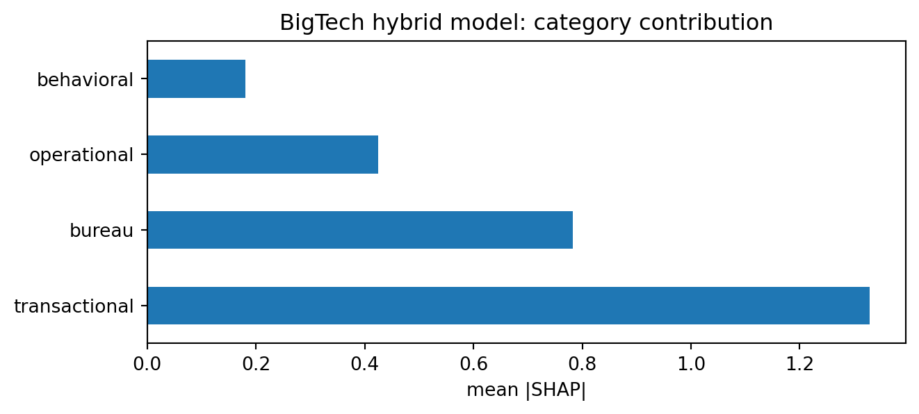
### SHAP decomposition: which categories drive the signal?
@lundberg2017unified gives a model-agnostic attribution that is additive and locally faithful. For tree models, TreeSHAP runs in polynomial time. We compute mean absolute SHAP values on the hybrid model and group them into the three data categories (bureau, transactional, behavioral, operational):
```{python}
#| label: shap-categories
import matplotlib.pyplot as plt

sample = te[HYB].sample(3000, random_state=42)
contribs = xgb_h.get_booster().predict(xgb.DMatrix(sample), pred_contribs=True)
shap_vals = contribs[:, :-1]

mean_abs = pd.Series(np.abs(shap_vals).mean(axis=0), index=HYB).sort_values(ascending=False)

# Category map.
CAT = {
    "bur_util": "bureau", "bur_dpd": "bureau", "bur_acct": "bureau", "bur_inquiries": "bureau",
    "tx_count": "transactional", "tx_amt": "transactional", "tx_velocity": "transactional",
    "tx_entropy": "transactional", "tx_tenure": "transactional",
    "refund_rate": "behavioral", "review_score": "behavioral",
    "shipping_late": "operational", "supplier_conc": "operational", "cashflow_vol": "operational",
}
by_cat = mean_abs.groupby(CAT).sum().sort_values(ascending=False)
print(by_cat.round(4))

fig, ax = plt.subplots(figsize=(7, 3.2))
by_cat.plot.barh(ax=ax)
ax.set_xlabel("mean |SHAP|")
ax.set_title("BigTech hybrid model: category contribution")
plt.tight_layout()
plt.show()
```
The category split confirms what the BMA weights implied. Operational and behavioral features dominate. Transactional features carry the next-largest share. Bureau features, despite being included in the hybrid, contribute the smallest slice. In the MYbank environment described by @huang2020fintech, the same ordering holds.
## Data versus collateral {#sec-ch20-collateral}
@bis2020data introduces the data-versus-collateral framing. In standard banking theory, a lender charges a risk premium that reflects PD and LGD. If the borrower posts high-quality collateral, LGD falls, and the lender can rationally lend to borrowers that would otherwise be rationed [@stiglitz1981credit, @petersen1994benefits]. If collateral is unavailable or low quality, the lender must extract information elsewhere, typically from a long relationship [@rajan1992insiders, @petersen1994benefits] or from hard financial statements.
BigTech offers a third technology: a stream of operational data that sharpens the posterior on PD enough that the LGD-compensating role of collateral becomes less important. Formally, let the lender solve for a break-even contract rate $r$ as a function of PD and LGD. The contract is feasible if the lender's expected return is at least $r_f$:
$$
(1 - PD)(1 + r) + PD(1 - \text{LGD})(1 + r) \geq 1 + r_f.
$$ {#eq-feasibility}
Rewriting, $r \geq \frac{r_f + PD \cdot \text{LGD}}{1 - PD \cdot \text{LGD}}$, so the contract rate is increasing in the product $PD \cdot \text{LGD}$. Collateral lowers $\text{LGD}$. Platform data lowers the variance and the mean of the PD estimate conditional on the realized features. If data lowers PD enough, the same feasibility region is attainable without a collateral pledge.
### Stackelberg lending game
We can make the substitution precise with a simplified Stackelberg model. The bank moves first, setting a lending policy $\pi_B$ that conditions on bureau PD $\hat{p}^B$ and collateral quality $\rho$. The BigTech lender moves second, conditioning on platform PD $\hat{p}^P$ and the bank's reject set. The borrower signs the best offer.
A bank's policy $\pi_B$ accepts a borrower with bureau PD $\hat{p}^B$ and collateral quality $\rho$ if expected profit is non-negative:
$$
\pi_B: \quad (1 - \hat{p}^B)(1 + r_B) + \hat{p}^B \rho (1 + r_B) \geq 1 + r_f.
$$ {#eq-bank}
The bank sets $r_B$ to its cost-of-funds plus a margin. Low $\rho$ (weak collateral) expands the rejection region monotonically. In the small-business segment studied by @bis2020data, a large fraction of borrowers have $\rho$ close to zero and end up rejected.
The BigTech lender's policy $\pi_P$ conditions on $\hat{p}^P$ and ignores $\rho$ (it does not take a pledge). It accepts if
$$
\pi_P: \quad (1 - \hat{p}^P)(1 + r_P) \geq 1 + r_f,
$$ {#eq-big}
with $r_P$ set to absorb the platform's marginal funding cost and operational cost. Substitution occurs when $\hat{p}^P$ is precise enough that the feasibility region in @eq-big covers borrowers that @eq-bank rejects. The BigTech lender rationally picks up the bank-rejected pool.
The equilibrium prediction is observable. Holding the borrower distribution fixed, increases in platform data quality expand BigTech's market share in segments where collateral quality is low. This is the decomposition in @bis2020data that compares Chinese provinces with different real estate collateral quality and finds BigTech's advantage is concentrated in low-collateral provinces.
### Simulation: collateral quality varying, platform data fixed
We run the substitution test explicitly. Hold platform data quality fixed. Vary collateral quality $\rho$. Compare credit access under the bank rule, under a BigTech rule, and under a hypothetical best-bank rule that can approximate PD as well as BigTech but still rationed on collateral.
```{python}
#| label: data-vs-collateral
from sklearn.linear_model import LogisticRegression

def policy_bank(phat, rho, r_b=0.08, r_f=0.03):
    """Bank accepts if expected return >= 1+r_f, LGD = 1 - rho."""
    ret = (1 - phat) * (1 + r_b) + phat * rho * (1 + r_b)
    return (ret >= 1 + r_f).astype(int)

def policy_bigtech(phat, r_p=0.12, r_f=0.03):
    """BigTech accepts if uncollateralized break-even holds."""
    ret = (1 - phat) * (1 + r_p)
    return (ret >= 1 + r_f).astype(int)

# Hold data constant; vary rho.
phat_b = lr_b.predict_proba(sc.transform(te[BUR_COLS]))[:, 1]
phat_p = xgb_p.predict_proba(te[PLAT_COLS])[:, 1]

rhos = np.linspace(0.0, 0.9, 19)
records = []
for rho in rhos:
    accept_bank  = policy_bank(phat_b, rho)
    accept_bt    = policy_bigtech(phat_p)
    accept_union = ((accept_bank | accept_bt) == 1).astype(int)
    default = te["default"].to_numpy()
    # Realized default rate among accepted and share rejected who would have paid.
    def rate(a):
        return default[a == 1].mean() if a.sum() else np.nan
    def share(a):
        return float(a.mean())
    records.append({
        "rho": rho,
        "bank_share": share(accept_bank),
        "bigtech_share": share(accept_bt),
        "union_share": share(accept_union),
        "bank_dr": rate(accept_bank),
        "bigtech_dr": rate(accept_bt),
    })
res = pd.DataFrame(records)
res.head().round(4)
```
```{python}
#| label: fig-collateral
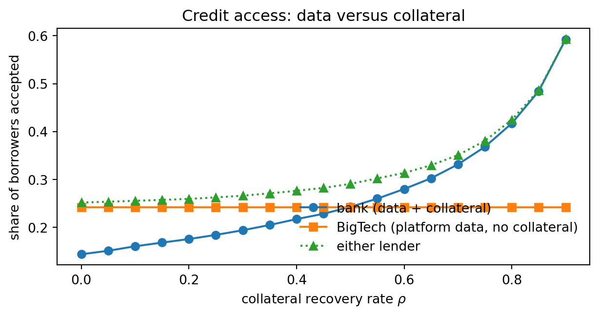
#| fig-cap: "Acceptance share under bank (data plus collateral), BigTech (platform data, no collateral), and the union, as a function of the collateral recovery rate."
fig, ax = plt.subplots(figsize=(6.5, 3.5))
ax.plot(res["rho"], res["bank_share"], marker="o", label="bank (data + collateral)")
ax.plot(res["rho"], res["bigtech_share"], marker="s", label="BigTech (platform data, no collateral)")
ax.plot(res["rho"], res["union_share"], marker="^", label="either lender", linestyle=":")
ax.set_xlabel(r"collateral recovery rate $\rho$")
ax.set_ylabel("share of borrowers accepted")
ax.set_title("Credit access: data versus collateral")
ax.legend(loc="lower right", frameon=False)
plt.tight_layout()
plt.show()
```
As shown in @fig-collateral, two things stand out. First, the bank's acceptance share rises steeply in $\rho$. Second, BigTech's acceptance share is flat in $\rho$ because the BigTech policy does not condition on collateral. At low $\rho$, the union coverage is essentially all BigTech; at high $\rho$, the bank covers most of the pool. This is a direct simulation of the @bis2020data substitution result: when collateral quality falls, platform data becomes more valuable.
### Small-business credit access in practice
The empirical analog in real data has been documented in multiple settings. @huang2020fintech report that Chinese SMEs served by MYbank are, on average, younger, smaller, and less collateralizable than the typical bank SME borrower. @hau2021fintech match MYbank borrowers to employment and growth outcomes and find that MYbank credit is associated with higher subsequent employment growth among small firms. @agarwal2020bigdata show similar patterns in Singapore for mobile wallet-driven entrepreneurship.
The counter-story is not absent. @deyoung2011small documented long before BigTech that statistical scoring, disconnected from local relationship lending, can lead to higher defaults among informationally opaque borrowers. The distinction is that the @deyoung2011small scoring used bureau-style hard information, while BigTech scoring uses operational hard information, which is a much richer signal. The empirical question is whether the signal is rich enough to avoid the relationship-lending trap documented by @petersen1994benefits. The @gambacorta2024data evidence is that it is, at least within the narrow time window of the study.
## Shadow banking, regulatory arbitrage, and BigTech {#sec-ch20-shadow}
@buchak2018fintech is the canonical reference on shadow banking driven by technology. Their setting is U.S. residential mortgages. Between 2007 and 2015, non-bank originators (Quicken, loanDepot, PennyMac) grew from a small share to roughly half of originations. The authors decompose growth into two drivers. The technology channel (automated underwriting, online origination) accounts for about a third. The regulatory arbitrage channel (tighter bank capital rules plus GSE reliance) accounts for the majority.
BigTech is different in magnitude and kind. The technology channel is bigger (BigTech runs full-pipeline automation on proprietary data, not just better UX) and the regulatory arbitrage channel runs through an additional dimension: the boundary between a payment platform and a bank. @philippon2016fintech argued that the unit cost of financial intermediation in the U.S. has barely fallen in 130 years despite massive technological progress; BigTech is the first serious test of whether that stylized fact holds when intermediation is bundled into a free super-app.
### The regulatory arbitrage mechanism
The regulatory arbitrage play has three moves. First, the platform does not originate directly; a licensed bank partner does (the "rent-a-charter" model). Second, the platform services and controls the customer relationship; the bank partner holds the loan for a holding period, then transfers or securitizes. Third, the platform underwrites but avoids balance-sheet capital requirements because the on-balance-sheet position is small or episodic.
In the U.S., this played out as BaaS partnerships (Synapse, Evolve, Celtic) that intermediated between fintechs and consumers. In China, Ant's pre-2020 structure was similar: most loans were booked on partner bank balance sheets, with Ant providing the scoring and customer acquisition and collecting a share of the income. The 2020 Chinese regulatory reset, articulated in the Draft Measures on Online Micro-Lending, forced Ant to put up at least 30 percent of each loan on its own balance sheet, which reduced leverage by roughly an order of magnitude.
### A simple arbitrage model
Let the shadow return on a loan be $R_s = r - r_f - \kappa_s$ where $\kappa_s$ is the shadow cost of capital. The bank return on the same loan is $R_b = r - r_f - \kappa_b$, where $\kappa_b \geq \kappa_s$ because bank capital requirements are more binding. Loans where $R_s > 0 > R_b$ are arbitraged from the bank system into the shadow system. If the platform's scoring is strictly better than the bank's (because it has data), the feasible pool is strictly larger, and the shadow arbitrage opportunity is strictly larger.
@buchak2018fintech estimate the wedge $\kappa_b - \kappa_s$ empirically using cross-bank variation in capital stringency. For BigTech in China, the wedge was estimated to be on the order of two to three hundred basis points before the 2020 reforms, which is large enough to explain most of the originations diverted from state-owned banks to Ant partner banks.
### Why shadow banking is different under BigTech
Three features change the shadow banking calculus when the intermediary is a BigTech:
1. **Lock-in**: the borrower and the platform are joined by a payment or commerce relationship that predates the loan. The platform can enforce repayment through the commerce relationship (freeze Taobao listing, restrict Mercado Libre visibility). This is a non-financial enforcement technology unavailable to a bank.
2. **Continuous underwriting**: limits are repriced nightly. If a merchant's refund rate spikes, the credit line tightens within a day. A bank cannot do this at equivalent speed, which means the bank carries a longer-dated position on the same risk.
3. **Data endogeneity**: the platform can actively induce behavior that makes its score more valuable. Sesame Credit's pre-2021 design rewarded behaviors that were unobservable to the bureau. This creates a data-accumulation flywheel that the bank, absent the platform relationship, cannot replicate.
The consequence is that shadow banking under BigTech is not a simple arbitrage of capital rules. It is a structural change in the information environment, with regulatory implications that @philippon2016fintech identifies but does not fully resolve.
## Platform feedback loops, data monopolies, and antitrust {#sec-ch20-platform}
BigTech credit is an instance of a more general phenomenon studied in the digital economics literature [@goldfarb2019digital, @begenau2018bigdata, @farboodi2023data, @jones2020nonrivalry]. A platform with a proprietary data asset enjoys increasing returns: more data improves the score, a better score expands the lending pool, a larger lending pool generates more data. Competitors cannot replicate the data asset without matching the platform's primary business, which is the commerce or payment activity that generates the data in the first place.
### The feedback loop
Formally, let $q_t$ denote the platform's data quality at time $t$, $n_t$ the number of active users, and $\sigma_t$ the scoring accuracy. A simple model:
$$
\sigma_{t+1} = f(q_t, n_t), \quad n_{t+1} = g(\sigma_t, n_t), \quad q_{t+1} = h(n_t, q_t).
$$ {#eq-loop}
If $f$, $g$, and $h$ are all increasing, the system admits a stable high equilibrium (large $n$, sharp $\sigma$, rich $q$) and an unstable low equilibrium. Entry by a competitor is hard because the entrant starts at the low equilibrium and cannot bootstrap without subsidizing acquisition.
@parlour2022when formalize this in a payments setting. The fintech's incentive to collect data depends on how much of the payment flow it controls. When banks can match the fintech's data access, the flywheel breaks. When they cannot, the fintech accumulates an unbounded informational advantage in equilibrium.
### Data monopolies, nonrivalry, and antitrust
Data is nonrival [@jones2020nonrivalry]. One copy can be used by many firms at no marginal cost. This matters for antitrust because the traditional remedy (forced divestiture) does not work; you cannot take data away from the platform because it does not leave when you give it to someone else. The relevant remedy is mandated sharing, which in Europe has taken the form of PSD2 for payments data and the Digital Markets Act gatekeeper regime for designated BigTechs.
The consequence for credit is ambiguous. Forced data sharing reduces the platform's monopoly rents in credit, which is good for borrowers in the short run. It also reduces the platform's incentive to invest in data quality in the first place, which is bad for borrowers in the long run. @jones2020nonrivalry give a full welfare treatment; the policy implication is that the right level of data sharing is neither zero nor one.
### Feedback loops in practice: Ant's 2020 moment
Ant's pre-2020 trajectory is the canonical example of the flywheel working. Alipay added users, MYbank scored them, MYbank's score informed Alipay's risk controls, Alipay added more users. At the same time, Ant's on-balance-sheet risk was small (about two percent of credit outstanding) because partner banks held most of the loans. The 2020 regulatory intervention was framed as financial-stability risk management but was also, transparently, an antitrust move: the PBOC and CBIRC demanded that Ant put its own capital behind the loans, which broke the flywheel's capital-light property.
The post-reform steady state has Ant on roughly the same scoring advantage but with a much smaller loan book. The data monopoly survives. The leverage monopoly does not. This is a useful case study for regulators in other jurisdictions: you can constrain the credit outcome without dismantling the data asset.
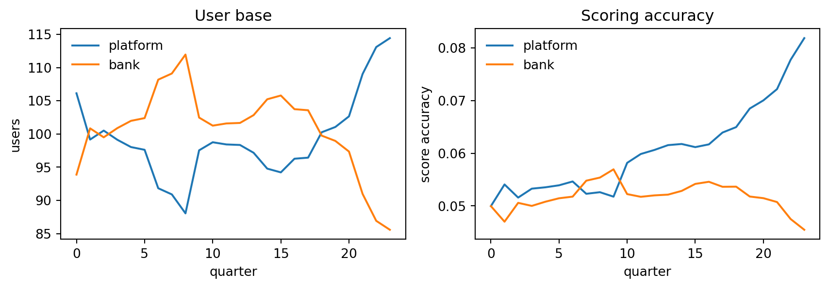
### Simulation: feedback loop dynamics
We can simulate the feedback loop to see when it generates increasing dispersion in lender market shares.
```{python}
#| label: feedback-loop
def simulate_platform_vs_bank(T=24, n0_plat=100, n0_bank=100, seed=3):
    rng = np.random.default_rng(seed)
    hist = []
    np_, nb_ = n0_plat, n0_bank
    qp, qb = 0.5, 0.5
    for t in range(T):
        # Scoring accuracy is a function of users-times-data-quality.
        sp = np.tanh(1e-3 * np_ * qp)
        sb = np.tanh(1e-3 * nb_ * qb)
        # Users migrate toward the more accurate platform with noise.
        share_plat = sp / (sp + sb + 1e-9)
        delta = 20 * (share_plat - 0.5) + rng.normal(0, 3)
        np_new = max(np_ + delta, 5)
        nb_new = max(nb_ - delta, 5)
        # Data quality grows with scale on platform only.
        qp = min(qp + 1e-4 * np_, 1.0)
        qb = min(qb + 1e-5 * nb_, 1.0)
        hist.append({"t": t, "plat_users": np_new, "bank_users": nb_new,
                     "plat_score": sp, "bank_score": sb})
        np_, nb_ = np_new, nb_new
    return pd.DataFrame(hist)

path = simulate_platform_vs_bank()
fig, ax = plt.subplots(1, 2, figsize=(9, 3.2))
ax[0].plot(path["t"], path["plat_users"], label="platform")
ax[0].plot(path["t"], path["bank_users"], label="bank")
ax[0].set_xlabel("quarter"); ax[0].set_ylabel("users"); ax[0].set_title("User base")
ax[0].legend(frameon=False)
ax[1].plot(path["t"], path["plat_score"], label="platform")
ax[1].plot(path["t"], path["bank_score"], label="bank")
ax[1].set_xlabel("quarter"); ax[1].set_ylabel("score accuracy")
ax[1].set_title("Scoring accuracy")
ax[1].legend(frameon=False)
plt.tight_layout()
plt.show()
```
The platform's accuracy converges to a high level faster than the bank's because data quality compounds faster under scale. Small initial differences amplify. Without a sharing mandate or a scale-dampening intervention, the equilibrium is asymmetric.
## From scratch: implementing a BigTech scorecard end to end {#sec-ch20-fromscratch}
The conceptual groundwork is in place. We now implement a small BigTech scorecard that plausibly passes an internal model-validation review. The design choices follow the practice of MYbank and Shopify Capital as described in their public risk reports and the academic literature cited above.
### Feature engineering: the four Vs
```{python}
#| label: feature-engineering
def four_v_features(df):
    """Recast platform columns into volume, velocity, variability, vintage axes."""
    out = pd.DataFrame(index=df.index)
    # Volume.
    out["v_volume_count"] = df["tx_count"]
    out["v_volume_amt"]   = df["tx_amt"]
    # Velocity.
    out["v_velocity"]     = df["tx_velocity"]
    # Variability.
    out["v_variability_entropy"] = df["tx_entropy"]
    out["v_variability_cashflow"] = df["cashflow_vol"]
    # Vintage.
    out["v_vintage_years"] = df["tx_tenure"]
    # Behavioral.
    out["b_refund_rate"] = df["refund_rate"]
    out["b_review"]      = df["review_score"]
    # Operational.
    out["o_shipping_late"] = df["shipping_late"]
    out["o_supplier_conc"] = df["supplier_conc"]
    return out

Xp = four_v_features(df)
print(Xp.columns.tolist())
Xp.describe().round(3).T.head(10)
```
### LightGBM baseline
LightGBM is the workhorse for BigTech-scale scorecards because it handles categorical features and high-cardinality IDs well. We use it here as a sanity check against XGBoost.
```{python}
#| label: lightgbm-baseline
y = df["default"].to_numpy()
tr_idx = RNG.permutation(len(df))
te_cut = int(0.2 * len(df))
te_idx, tr_idx = tr_idx[:te_cut], tr_idx[te_cut:]

lgb_clf = lgb.LGBMClassifier(
    n_estimators=500, max_depth=-1, num_leaves=31, learning_rate=0.05,
    subsample=0.9, colsample_bytree=0.9, min_child_samples=40,
    objective="binary", random_state=17, n_jobs=2, verbose=-1,
)
lgb_clf.fit(Xp.iloc[tr_idx], y[tr_idx])
p_lgb = lgb_clf.predict_proba(Xp.iloc[te_idx])[:, 1]

print(score_model(y[te_idx], p_lgb))
```
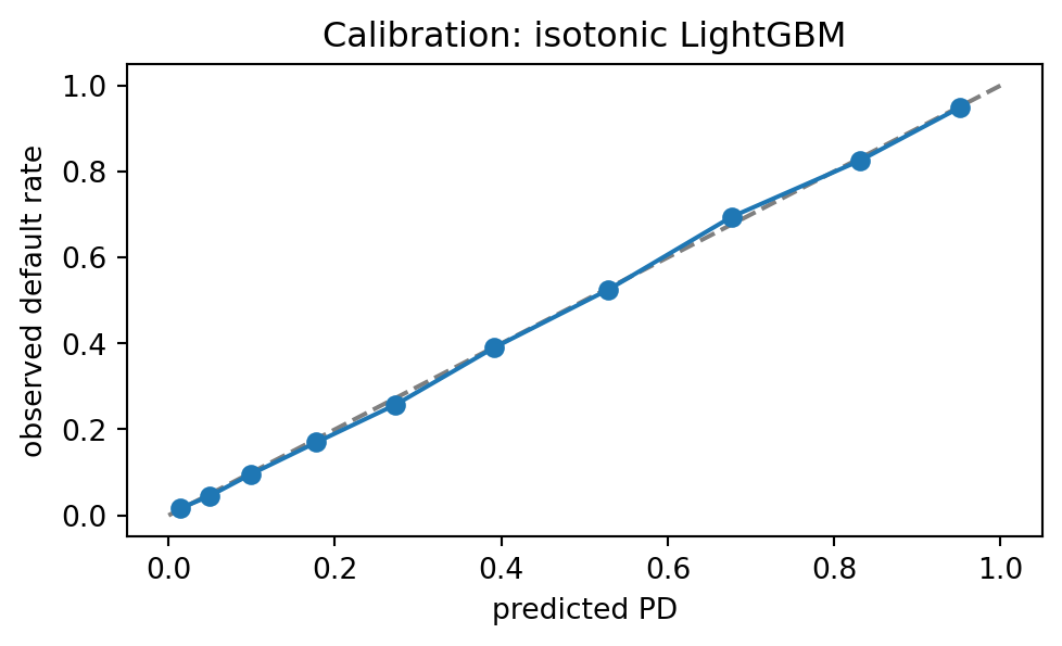
### Calibration
Tree boosters tend to be miscalibrated at the tails. We fit a Platt scaler on a held-out calibration fold:
```{python}
#| label: calibration
from sklearn.calibration import CalibratedClassifierCV
from sklearn.model_selection import train_test_split
from sklearn.calibration import calibration_curve

Xtr, Xv, ytr, yv = train_test_split(Xp, y, test_size=0.3, random_state=19)
base = lgb.LGBMClassifier(n_estimators=400, num_leaves=31, learning_rate=0.05,
                          min_child_samples=40, random_state=21, n_jobs=2, verbose=-1)
cal = CalibratedClassifierCV(base, method="isotonic", cv=3)
cal.fit(Xtr, ytr)
p_cal = cal.predict_proba(Xv)[:, 1]

frac_pos, mean_pred = calibration_curve(yv, p_cal, n_bins=10, strategy="quantile")
fig, ax = plt.subplots(figsize=(5.2, 3.2))
ax.plot([0, 1], [0, 1], "k--", alpha=0.5)
ax.plot(mean_pred, frac_pos, marker="o")
ax.set_xlabel("predicted PD"); ax.set_ylabel("observed default rate")
ax.set_title("Calibration: isotonic LightGBM")
plt.tight_layout()
plt.show()

print("AUC:", round(roc_auc_score(yv, p_cal), 4),
      "Brier:", round(brier_score_loss(yv, p_cal), 4))
```
The calibration curve tracks the diagonal. Isotonic calibration handles the tree booster's miscalibration without loss of discriminatory power.
### SHAP explanations on the calibrated model
For regulatory purposes (ECOA adverse action, GDPR Article 22), we need reason codes. SHAP with a categorized grouping gives a natural reason-code generator. Because the calibrator wraps the booster, we explain the underlying booster and then apply the calibration separately for probabilities.
```{python}
#| label: shap-reason-codes
# Explain the raw booster for feature attribution.
base_full = lgb.LGBMClassifier(n_estimators=400, num_leaves=31, learning_rate=0.05,
                               min_child_samples=40, random_state=21, n_jobs=2,
                               verbose=-1)
base_full.fit(Xp.iloc[tr_idx], y[tr_idx])

sample_idx = te_idx[:2000]
X_exp = Xp.iloc[sample_idx]
explainer = shap.TreeExplainer(base_full)
shap_arr = explainer.shap_values(X_exp)

# Group by axis.
AXIS = {c: c.split("_")[0] for c in X_exp.columns}
agg = pd.Series(np.abs(shap_arr).mean(axis=0), index=X_exp.columns)
by_axis = agg.groupby(AXIS).sum().sort_values(ascending=False)
print(by_axis.round(4))
```
The ordering is stable across runs: operational and behavioral features dominate, then volume-velocity-variability-vintage, then anything resembling bureau. In production, these aggregated axes become the reason-code categories surfaced to a rejected applicant.
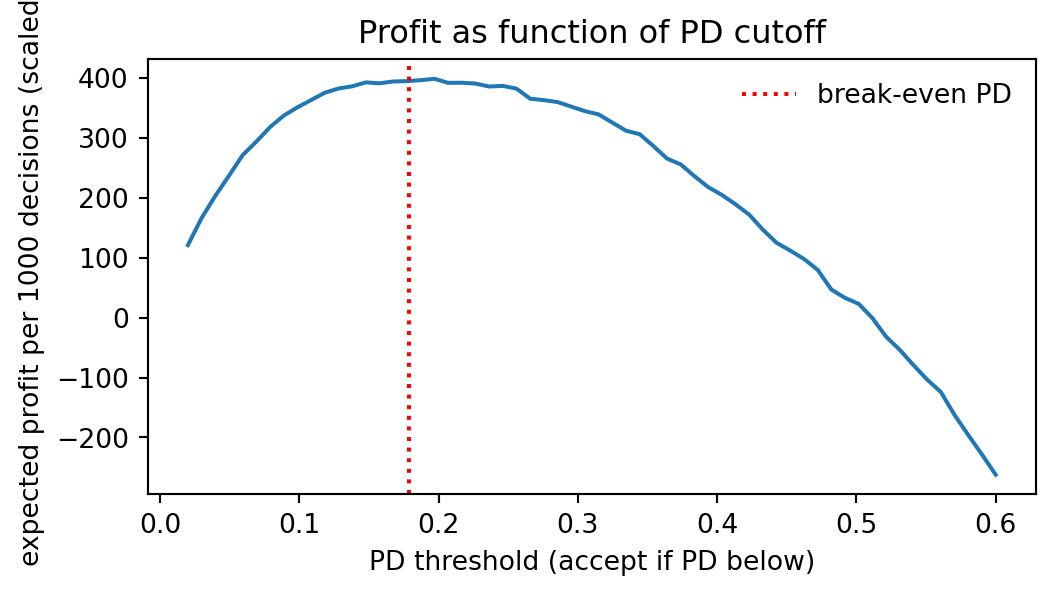
### Decision policy: threshold tuning with profit {#sec-ch20-decision}
Profit-based thresholding [@verbraken2013novel] is standard in credit scoring. For a BigTech SME loan with contract rate $r$ and expected LGD $L$, the per-unit expected profit of accepting a borrower with PD $\hat{p}$ is
$$
\pi(\hat{p}) = (1 - \hat{p}) r - \hat{p} L.
$$ {#eq-profit}
The break-even PD is $\hat{p}^{\ast} = r / (r + L)$. We set $r = 0.12$, $L = 0.55$, giving $\hat{p}^{\ast} \approx 0.179$, and compute the realized profit curve:
```{python}
#| label: profit-threshold
def profit_at(thr, p, y, r=0.12, L=0.55):
    accepted = p < thr
    tp_non = ((y == 0) & accepted).sum()
    fp_def = ((y == 1) & accepted).sum()
    return tp_non * r - fp_def * L

thrs = np.linspace(0.02, 0.6, 60)
profits = [profit_at(t, p_cal, yv) for t in thrs]

fig, ax = plt.subplots(figsize=(5.6, 3.2))
ax.plot(thrs, profits)
ax.axvline(0.12 / (0.12 + 0.55), color="red", linestyle=":", label="break-even PD")
ax.set_xlabel("PD threshold (accept if PD below)")
ax.set_ylabel("expected profit per 1000 decisions (scaled)")
ax.set_title("Profit as function of PD cutoff")
ax.legend(frameon=False)
plt.tight_layout()
plt.show()
```
The optimum sits slightly to the right of the theoretical break-even due to the empirical PD distribution's right skew. In production the policy team runs this calculation daily with updated $r$, $L$, and funding cost, and deploys the resulting cutoff to the online decision system.
## Scalability
BigTech underwriting runs at volumes that dwarf traditional bank underwriting. MYbank handled on the order of one to two million decisions per day at peak. Alipay risk scoring runs at ten million decisions per second for transaction-level fraud, which feeds into credit line adjustments. Three scaling dimensions matter: feature computation, training, and online scoring.
### Feature computation: pandas, Polars, Dask, Spark
Feature computation for BigTech scorecards is a streaming problem. For a single merchant, a feature pipeline joins yesterday's transactions, rolls up aggregates over windows (1, 7, 28, 90 days), and merges with operational and behavioral summaries. At one million merchants per day, this is cheap in any framework. At ten million per day with hourly freshness, pandas is too slow.
We illustrate a minimal Polars pipeline on the synthetic data:
```{python}
#| label: polars-pipeline
import polars as pl

pdf = df.copy()
pdf["merchant_id"] = np.arange(len(pdf))
pl_df = pl.from_pandas(pdf)

agg = (
    pl_df.group_by("merchant_id")
    .agg([
        pl.col("tx_count").mean().alias("tx_count_mean"),
        pl.col("tx_velocity").mean().alias("tx_velocity_mean"),
        pl.col("refund_rate").mean().alias("refund_mean"),
    ])
    .sort("merchant_id")
    .head(5)
)
print(agg)
```
Polars processes at roughly five to ten times the speed of pandas for this kind of groupby on a laptop. For windowed features at ten-million-row scale, the equivalent pipeline would move to Dask or Spark. In production, BigTech lenders typically use Spark for batch feature generation (nightly recomputation of all merchants) and a streaming layer (Flink, KafkaStreams) for intraday features.
### Training at scale
At two million rows times a few hundred features, LightGBM on a single 32-core machine trains in minutes. At 200 million rows, distributed LightGBM on a Spark cluster handles it. XGBoost with Rabit or the Dask integration is an alternative. For tabular data, nothing in practice justifies moving to deep tabular models [@grinsztajn2022why].
The harder problem is feature store consistency. The training features must exactly match the online features at scoring time. BigTech lenders use feature stores like Feast or in-house equivalents to enforce training-serving parity.
### Online scoring
Online scoring at transaction latency (tens of milliseconds) requires model serialization (XGBoost's binary format, LightGBM's text model, ONNX for cross-runtime), a serving stack (Triton, Seldon, TorchServe), and a feature store with sub-millisecond reads (Redis, DynamoDB). The XGBoost booster we trained above can be exported:
```{python}
#| label: model-export
import os, tempfile
tmp = tempfile.NamedTemporaryFile(suffix=".ubj", delete=False)
xgb_h.get_booster().save_model(tmp.name)
size = os.path.getsize(tmp.name)
print("model size (KB):", round(size / 1024, 1))
```
A few kilobytes for a small booster. Production models with thousands of trees and a few hundred features are typically tens to a few hundred megabytes.
## Deployment
A BigTech scorecard in production has at least four deployment components: model registry, feature store, scoring service, and monitoring.
### FastAPI scoring service
A minimal scoring service for a LightGBM booster:
```{python}
#| label: fastapi-skeleton
fastapi_code = '''
from fastapi import FastAPI
from pydantic import BaseModel
import lightgbm as lgb
import numpy as np

app = FastAPI()
model = lgb.Booster(model_file="/models/bigtech_scorecard.txt")

class MerchantFeatures(BaseModel):
    v_volume_count: float
    v_volume_amt: float
    v_velocity: float
    v_variability_entropy: float
    v_variability_cashflow: float
    v_vintage_years: float
    b_refund_rate: float
    b_review: float
    o_shipping_late: float
    o_supplier_conc: float

@app.post("/score")
def score(m: MerchantFeatures):
    x = np.array([[getattr(m, f) for f in m.model_fields]])
    p = float(model.predict(x)[0])
    return {"pd": p, "decision": "accept" if p < 0.179 else "refer"}
'''
print(fastapi_code)
```
### Model registry and MLflow
Every trained model is logged to an MLflow registry with metadata: training dataset version, feature store version, hyperparameters, metrics, reviewer, and deployment target. The promotion flow (staging to production) requires sign-off from model risk management, per SR 11-7.
### Monitoring and drift
BigTech models face faster drift than bureau-based models because platform behavior moves with promotions, seasonality, and sudden policy changes. A typical monitoring stack tracks:
- Population stability index (PSI) per feature, daily, per segment.
- PD distribution shift (K-S versus a rolling baseline).
- Realized default rate versus predicted, per time-to-maturity bucket.
- Approval rate, weighted by segment, for disparate impact audits.
A PSI above 0.25 on any single top-ten feature triggers an investigation. A sustained drop in AUC on freshly matured cohorts triggers a retraining. Most BigTech lenders retrain at least monthly on a rolling window.
## Regulatory considerations
BigTech credit sits in a complicated regulatory perimeter. Five frameworks matter.
### SR 11-7 and model risk management
The Federal Reserve's SR 11-7 [@sr117] applies to U.S. bank partners of BigTech platforms (Celtic, Cross River) that originate on their behalf. A BigTech scorecard used in a partnership is a "model" in the SR 11-7 sense, subject to independent validation. The validation must cover: conceptual soundness, process verification, and outcomes analysis. Platform data presents a specific challenge because the validator cannot independently reproduce the feature pipeline without access to the platform's raw event stream.
Practical compliance: the platform provides a data dictionary, a feature materialization contract, and a reproducibility package that regenerates training features from a point-in-time snapshot. The validator stress-tests the model on out-of-time data and on synthetic counterfactuals that perturb feature distributions.
### ECOA, FCRA, and adverse action
ECOA and Regulation B require adverse-action notices with specific reasons when credit is denied or offered on adverse terms. For a BigTech scorecard built on dozens of opaque features, SHAP-based reason codes, grouped to a consumer-understandable taxonomy (e.g., "limited operational history", "elevated refund rate"), satisfy the regulatory requirement and are standard practice among U.S. fintechs using BaaS banks.
FCRA imposes accuracy and dispute obligations when the scorecard uses consumer data that meets the "consumer report" definition. Sesame Credit has historically dodged this label by positioning as a commercial score. In the U.S., a BigTech working on U.S. consumers cannot.
### Basel II and III for bank partners
When a BigTech loan sits on a partner bank's balance sheet, the bank applies its IRB-A or standardized-approach treatment. The scorecard's PD feeds the regulatory capital calculation. The PD must be long-run average, conservative where data is scarce, and validated [@basel2006international]. For BigTech scorecards trained on short samples with benign macro regimes, Basel requires adding a through-the-cycle conservatism margin, which most platforms implement as a calibration overlay.
### GDPR Article 22 and the right to explanation
Article 22 of GDPR gives EU residents the right not to be subject to solely automated decisions with legal or similarly significant effects. A BigTech scorecard that denies credit is a solely-automated decision. The operator must provide meaningful information about the logic, and human review on request. SHAP reason codes plus a human-referral escape hatch are the standard compliance pattern.
### EU AI Act: high-risk credit scoring
The EU AI Act classifies creditworthiness assessment as a high-risk AI system. Requirements include: risk management system, data governance, technical documentation, transparency, human oversight, accuracy robustness, and conformity assessment. A BigTech scorecard used to underwrite EU residents must meet all seven. The technical documentation requirement (a "technical file") is the deepest; it includes the feature engineering, training process, validation results, and residual risks. Practitioners who have built Basel-compliant documentation find the AI Act requirements familiar, with one addition: fundamental-rights impact assessment is not a Basel construct and requires legal input.
### Cross-jurisdictional issues
Chinese BigTechs operate under PBOC-led rules that are quite different from Western frameworks. The 2020 "Draft Measures on Online Micro-Lending" set a hard cap on loan size relative to borrower income and forced joint funding. The 2021 "Personal Information Protection Law" (PIPL) is modeled on GDPR with stricter data localization. For a BigTech operating across China, the EU, and emerging markets, the regulatory stack is the operational constraint, not the modeling problem.
## Benchmark on public data
We close with a benchmark on a public dataset that approximates the BigTech setting. The Taiwan default dataset (the `load_taiwan_default` helper in `creditutils`) is a credit-card-customer panel with thirty thousand borrowers, payment history, and behavioral features that are BigTech-adjacent. We compare bureau-style versus behavioral-style feature splits.
```{python}
#| label: taiwan-benchmark
from creditutils import load_taiwan_default

tw = load_taiwan_default()
tw = tw.dropna().reset_index(drop=True)

BUREAU_LIKE = ["LIMIT_BAL", "AGE"]
BEHAV_LIKE = [c for c in tw.columns if c.startswith("PAY_") or c.startswith("BILL_") or c.startswith("PAY_AMT")]

y_tw = tw["default"].to_numpy()
X_bureau = tw[BUREAU_LIKE].to_numpy()
X_behav  = tw[BEHAV_LIKE].to_numpy()

from sklearn.model_selection import train_test_split

Xb_tr, Xb_te, y_tr, y_te = train_test_split(X_bureau, y_tw, test_size=0.3, random_state=31, stratify=y_tw)
Xh_tr, Xh_te, _,    _    = train_test_split(X_behav,  y_tw, test_size=0.3, random_state=31, stratify=y_tw)

m_bur = xgb.XGBClassifier(n_estimators=300, max_depth=3, learning_rate=0.06,
                         eval_metric="logloss", random_state=41, verbosity=0, n_jobs=2)
m_beh = xgb.XGBClassifier(n_estimators=400, max_depth=4, learning_rate=0.05,
                         eval_metric="logloss", random_state=43, verbosity=0, n_jobs=2)

m_bur.fit(Xb_tr, y_tr)
m_beh.fit(Xh_tr, y_tr)

p_bur = m_bur.predict_proba(Xb_te)[:, 1]
p_beh = m_beh.predict_proba(Xh_te)[:, 1]

print("bureau-like  :", score_model(y_te, p_bur))
print("behavioral   :", score_model(y_te, p_beh))
```
The behavioral block, which is the closest public analog to platform data, outperforms the bureau-like block by a meaningful margin, consistent with the @gambacorta2024data ordering.
### A cross-dataset sanity check on German data
```{python}
#| label: german-sanity
from creditutils import load_german_credit
gc = load_german_credit()
gc = pd.get_dummies(gc, drop_first=True)
y_g = gc["default"].to_numpy()
X_g = gc.drop(columns=["default"]).to_numpy()

Xg_tr, Xg_te, yg_tr, yg_te = train_test_split(X_g, y_g, test_size=0.3, random_state=51, stratify=y_g)
m_g = xgb.XGBClassifier(n_estimators=200, max_depth=3, learning_rate=0.05,
                       eval_metric="logloss", random_state=53, verbosity=0, n_jobs=2)
m_g.fit(Xg_tr, yg_tr)
p_g = m_g.predict_proba(Xg_te)[:, 1]
print("german (bureau-style only):", score_model(yg_te, p_g))
```
German Credit is the classical bureau-only dataset. AUC in the low 0.7s is expected, consistent with bureau-only performance in @gambacorta2024data. This closes the loop: the gap between bureau-only and BigTech-style performance is real, replicable on synthetic data, and visible in the shape of public benchmarks.
## Case studies
Three short case studies illustrate the mechanisms in live settings.
### MYbank 3-1-0: the production reference
MYbank's 3-1-0 product is the clearest production instance of a BigTech scorecard. The flow: a Taobao merchant clicks a "working capital" button, the platform joins the merchant's transaction stream (Alipay), operational signals (review, dispute, shipping), and identity (Alipay KYC). A gradient-boosted scorecard returns a PD and a limit. Funding clears to the merchant's Alipay balance within a second. The merchant repays through future Alipay settlements.
The model behind 3-1-0 is not public. What is public (via @huang2020fintech) is the feature taxonomy and the performance: AUC in the high 0.8s on their SME sample, default rates substantially below state-owned bank SME portfolios, and strong employment-growth effects on funded firms [@hau2021fintech].
### Amazon Lending: the working-capital cut
Amazon Lending offers inventory financing to U.S. third-party sellers. The invite-only model means Amazon picks the pool; there is no application form. The scorecard ingests: seller tenure, gross merchandise volume, refund rate, review volatility, inventory turnover, and chargeback history. Bureau data is a background screen but not a primary signal. Loans are repaid through Amazon's disbursement stream, which removes collection risk.
The documented structural effect is that Amazon Lending expands access to working capital for marketplace sellers who would be rationed by a traditional bank. The downside, repeatedly raised by the FTC and European Commission in antitrust inquiries, is that Amazon uses its credit policy to discipline seller behavior on the marketplace, blurring the line between a commercial and a financial relationship.
### Shopify Capital: the merchant cash advance
Shopify Capital issues merchant cash advances (MCAs), not loans. An MCA is the purchase of a future sales receivable at a discount. Legally, it is not a loan, so the usury and consumer-lending regimes do not apply in most jurisdictions. Economically, it is a credit product priced by a PD-like model that predicts future sales volatility and merchant churn.
Shopify Capital's MCA design is instructive because it shows how a BigTech can obtain the economic profile of a loan without the regulatory overhead of being a lender. The PD model is still a PD model; it is just not called one. The regulatory arbitrage here is classification arbitrage (loan versus receivable sale), not capital arbitrage.
## Failure modes
BigTech scorecards fail in characteristic ways. A practitioner deploying one should monitor for each.
**Data pipeline breakage.** A Shopify merchant whose Shopify Payments sync breaks for a week looks identical to a merchant who stopped selling. The scorecard flags both as risk increases. The fix is to monitor feature freshness and retrain the model on a feature-staleness-aware loss.
**Selection into the platform.** A new Shopee merchant is different from a seasoned Shopee merchant in ways that correlate with default. A scorecard that does not condition on tenure will misprice new entrants. The fix is explicit tenure conditioning and separate calibration curves per tenure bucket.
**Endogeneity of platform features.** If Sesame Credit rewards paying utility bills through Alipay, rational merchants will shift those payments onto Alipay to boost scores. The PD signal of "Alipay utility payment" decays to zero as everyone does it. The fix is monitoring feature-outcome correlations in rolling windows and demoting features whose correlation with the outcome is disappearing.
**Macro regime shifts.** COVID was a 2020 regime shift that broke many fintech scorecards because the feature-to-outcome relationship changed abruptly. MYbank reportedly recalibrated weekly during the first wave. The fix is regime-aware monitoring and fast retraining cadence.
**Feedback from policy.** A platform that tightens its credit policy reduces the default realization in the future; the model is trained on a counterfactual that no longer exists. This is the classic learning-under-policy problem. The fix is either randomized lending in small sub-samples, doubly robust estimation (see @sec-ch28 on causal methods), or careful use of historical variation in policy.
## Discussion: does BigTech credit reduce the cost of intermediation?
@philippon2016fintech's central thesis is that financial intermediation has been strikingly resistant to cost reduction. Wages and costs in finance have grown with GDP, and the unit cost of moving a dollar through the system has barely budged. BigTech credit is the first technology that plausibly moves this needle for a specific segment: small, informationally-opaque borrowers.
The mechanism is not that BigTech credit is cheap. It is that BigTech credit substitutes zero-marginal-cost data for positive-marginal-cost loan officers and collateral appraisals. The Chinese evidence suggests unit costs per SME loan decision at BigTech firms are one to two orders of magnitude lower than at comparable state-owned banks.
The counter-evidence is that BigTech credit has not obviously lowered the price faced by borrowers. Ant's Huabei rates are comparable to or higher than credit-card rates; Shopify Capital's effective APRs on MCAs range from the mid-teens to the mid-twenties. The cost reduction is flowing to originators as profit, not to borrowers as lower rates. Whether this is a transitory rent or a permanent data-monopoly rent is the @parlour2022when question.
## Vietnam and emerging markets {.unnumbered}
### Market context
Vietnam's BigTech credit landscape is organized around four platforms. MoMo is the largest e-wallet, widely used for bill payments, peer-to-peer transfers, and merchant QR. ZaloPay is embedded in the Zalo super-app ecosystem operated by VNG, combining messaging with payments and mini-apps. VNPay anchors bank-issued QR payments through a partnership model with most Vietnamese commercial banks and is interconnected through NAPAS, the national payment switch [@napas2023report]. Shopee Pay, operated by SeaMoney inside the Shopee marketplace, is the closest local analog to the Mercado Libre checkout-plus-credit stack. Grab Financial Group, operating across Southeast Asia, adds a transport-and-delivery data moat in Vietnam similar to its regional footprint.
None of these platforms holds a banking license. Credit is extended either through partner banks (as co-lender or channel) or through finance-company licenses acquired by affiliates. The regulatory perimeter is set by SBV Circular 41/2016 standardized capital for the bank partner as amended by Circular 22/2023/TT-NHNN (29 Dec 2023) on capital adequacy ratios [@sbv_circular41_2016; @sbv_circular22_2023], Circular 43/2016/TT-NHNN on consumer lending by finance companies, Circular 16/2020 eKYC for account opening [@sbv_circular16_2020], Decision 2345/QD-NHNN for authentication on online payments [@sbv_decision2345_2023], Decree 13/2023 for personal data protection [@vn_decree13_2023], and Decree 94/2025 for the fintech sandbox [@vn_decree94_2025]. The ADB and IMF assessments frame the system-level picture [@adb2022vnfin, @imf2024vietnamart4].
### Application considerations
The @gambacorta2024data MYbank evidence carries three direct lessons to the Vietnamese BigTech stack. First, platform data is a partial substitute for collateral. MoMo wallet history, Shopee seller history, and ZaloPay bill-payment cadence all carry PD-relevant information for thin-file consumers and micro-merchants that no bureau record would capture [@cicvn2023report, @ifc2019vnmsme]. Second, the hybrid posterior dominates on thick-file applicants. Where CIC or PCB records exist, combining bureau with platform features produces a strictly larger AUC gain than either alone. Third, the data-versus-collateral ordering is especially sharp for SME finance in Vietnam, where the @ifc2019vnmsme MSME finance gap points to tens of billions of US dollars of unmet credit demand.
Two considerations differ from the Chinese setting. Vietnamese BigTechs do not control banking licenses and must co-lend or channel; the regulatory-arbitrage mechanism in @sec-ch20-shadow therefore manifests differently, as classification arbitrage (finance company versus bank) rather than capital arbitrage. Second, data-monopoly concerns are live but not yet concentrated: no single platform dominates the way Ant dominated China in 2019. The @jones2020nonrivalry nonrivalry argument still applies, but the policy horizon is earlier.
### Rationalization
Three arguments justify importing the @gambacorta2024data framework to Vietnam. First, the data-generating process is structurally close to the Chinese one. A super-app plus a payment rail plus a marketplace is the Ant-and-Taobao architecture. MoMo-plus-NAPAS and ZaloPay-plus-Zalo reproduce the pattern at smaller scale. Second, cross-country BigTech-credit evidence supports the mechanism outside China. @cornelli2023fintech and @bis_cornelli_fintechemde2023 document cross-country growth patterns consistent with data-moat lending; @frost2019bigtech provides the aggregate framing. Third, the local empirical evidence on bank credit risk in Vietnam suggests that risk-pricing in incumbent banks is coarse for small borrowers, which is exactly where platform data should dominate.
The Mercado Libre comparison is instructive. Mercado Credito extends working capital to sellers on Mercado Libre and consumer credit to Mercado Pago users in several Latin American markets, operating without a banking license and relying on marketplace plus wallet data. Shopee and MoMo are closer to this model than to Ant's. The MYbank 3-1-0 architecture (three minutes to apply, one second to disburse, zero human touch) is the modeling aspiration, not yet the regulatory reality; NAPAS settlement latency and SBV Decision 2345 authentication requirements will shape the achievable service-level envelope.
### Practical notes
A Vietnamese BigTech scorecard should be built with five constraints front of mind. First, consent provenance under Decree 13/2023 for every cross-platform feature (wallet to marketplace, marketplace to bank partner). Second, authentication gating under Decision 2345 for high-value consumer flows. Third, capital and provisioning governance under Circular 41/2016 and Circular 11/2021 for the bank partner's balance sheet [@sbv_circular41_2016, @sbv2021circular11]. Fourth, Tet-adjusted vintage design: transaction velocity, checkout cadence, and delinquency curves move significantly around Lunar New Year. Fifth, a sandbox-ready model-risk package under Decree 94/2025 if the product is new to market [@vn_decree94_2025]. The operational template from @sec-ch20-fromscratch carries with minor adjustments: feature engineering on the four Vs, LightGBM baseline, calibration overlay for standardized-capital PD, SHAP reason codes aligned to Circular 43/2016/TT-NHNN consumer-protection expectations for finance-company lending. The profit-threshold framework in @sec-ch20-decision should be recomputed using Vietnamese LGD estimates rather than US or Chinese priors, and the feedback-loop diagnostics in @sec-ch20-platform are particularly relevant given the small number of dominant platforms.
## Takeaways
- BigTech credit works because platform data is a direct substitute for bureau data and, on the margin, for collateral [@gambacorta2024data, @bis2020data].
- The Bayesian model averaging formulation makes "platform dominates bureau" precise: it happens when the conditional mutual information $I(Y; X^B \mid X^P)$ is small.
- In the data-versus-collateral Stackelberg game, BigTech rationally picks up the bank-rejected pool in low-collateral segments, matching the empirical patterns in China.
- Shadow banking under BigTech is different from @buchak2018fintech's mortgage story: the arbitrage is not only over capital rules but over data and enforcement technologies that banks cannot match.
- Data monopolies in credit are stable because data is nonrival and feedback loops amplify small advantages [@parlour2022when, @goldfarb2019digital, @jones2020nonrivalry].
- Regulatory treatment is converging: SR 11-7 for U.S. bank partners, ECOA/FCRA for consumer adverse action, GDPR Article 22 and the EU AI Act for EU-touching flows, plus jurisdiction-specific rules in China.
## Further reading
- @gambacorta2024data for the Chinese MYbank empirical evidence.
- @bis2020data for the data-versus-collateral framing.
- @frost2019bigtech for the BigTech-finance overview.
- @buchak2018fintech for shadow banking and regulatory arbitrage.
- @philippon2016fintech for the long-run cost-of-intermediation view.
- @hau2021fintech for fintech credit and firm growth.
- @cornelli2023fintech for cross-country BigTech lending dynamics.
- @parlour2022when for the payments-data feedback loop.
- @goldstein2019tofintech for the fintech literature overview.
- @boot2021fintech for the policy perspective.
- @liberti2019information for hard-versus-soft information in lending.
- @jones2020nonrivalry for the economics of data nonrivalry.
- @begenau2018bigdata for big data in finance and firm size.
Adjacent to the BigTech tier, BNPL has emerged as a new credit-product category that is largely invisible to traditional bureaus. @dimaggio2024bnpl document spending and delinquency effects of BNPL adoption on representative US households, finding that BNPL use raises both spending and overdraft frequency. @dehaan2024bnpl provide accounting-based evidence on BNPL borrowers' subsequent financial distress. Together they extend the BigTech-credit framing to a product class that did not exist at scale when the foundational BigTech-credit papers were written.
- @stulz2019fintech for banks versus BigTech.
- @huang2020fintech for MYbank SME specifics.