---
execute:
echo: true
eval: true
---
# Mathematical Prerequisites {#sec-app-A}
## What this appendix does {.unnumbered}
This appendix is a compact refresher of the mathematics used throughout the book. It is not a textbook. The goal is to give a reader who has seen this material before, perhaps years ago, a single place to look up the exact definition, inequality, or algorithm invoked in a chapter, with notation that matches the rest of the book. Every result is stated precisely, almost every result is proved in a line or two or cited to a standard source, and the core computational objects (CLT simulation, SVD, KKT system, IRLS for logistic regression, bootstrap AUC) are implemented from scratch so that the reader can rerun them and trust the formulas.
The scope is deliberate. We want the reader who is doing credit scoring work to reason correctly about probabilities, calibrated scores, and regularized GLMs. We want them to know why a positive definite matrix is safe to Cholesky factor, why IRLS converges for the logistic loss, why the bootstrap confidence interval for AUC is valid, and what "ignorability" buys in a causal analysis. Anything beyond that is out of scope and left to the references at the end. Chapters defer to this appendix by tag: probability to @sec-app-A-math, linear algebra to @sec-la, convex optimization to @sec-opt, information theory to @sec-info, inference to @sec-inf, causality to @sec-causal, and survival to @sec-surv.
Notation conventions are fixed once here. Random variables are capitalized ($X, Y, Z$), realizations lowercase ($x, y, z$), vectors bold lowercase ($\mathbf{x}, \mathbf{\beta}$), matrices bold uppercase ($\mathbf{X}, \mathbf{A}$). The symbol $\mathbb{E}$ denotes expectation, $\mathrm{Var}$ variance, $\mathrm{Cov}$ covariance, $\mathbb{P}$ probability. Log is natural log. Indicators are $\mathbb{1}\{\cdot\}$. The positive default in a regression context is "default event", denoted $Y=1$.
## Probability and measure {#sec-app-A-math}
### Probability spaces and random variables
A probability space is a triple $(\Omega, \mathcal{F}, \mathbb{P})$ where $\Omega$ is a sample space, $\mathcal{F}$ is a $\sigma$-algebra of measurable events, and $\mathbb{P}$ is a probability measure. A random variable $X$ is an $\mathcal{F}$-measurable function $X: \Omega \to \mathbb{R}$. In credit scoring, $\Omega$ is "all applications or accounts in some population", $\mathcal{F}$ is whatever subset structure we declare, and the default indicator $Y(\omega) \in \{0,1\}$ is the workhorse random variable. Detailed measure-theoretic background is in @billingsley1995probability.
The distribution of $X$ is the pushforward $\mathbb{P}_X(B) = \mathbb{P}(X \in B)$ for Borel sets $B$. When $X$ admits a density $f_X$ with respect to Lebesgue measure, $\mathbb{P}(X \in B) = \int_B f_X(x)\,dx$. When $X$ is discrete, $\mathbb{P}_X$ is a probability mass function (pmf) $p_X$.
### Expectation, variance, covariance
Expectation is a Lebesgue integral,
$$
\mathbb{E}[X] = \int_\Omega X(\omega)\,d\mathbb{P}(\omega),
$$ {#eq-exp}
defined whenever $\mathbb{E}|X| < \infty$. Linearity $\mathbb{E}[aX+bY] = a\mathbb{E}[X] + b\mathbb{E}[Y]$ holds under integrability. The variance and covariance are
$$
\mathrm{Var}(X) = \mathbb{E}[(X - \mathbb{E}[X])^2],
\qquad
\mathrm{Cov}(X, Y) = \mathbb{E}[(X - \mathbb{E}[X])(Y - \mathbb{E}[Y])].
$$ {#eq-var}
For a random vector $\mathbf{X} \in \mathbb{R}^p$ with mean $\mathbf{\mu} = \mathbb{E}[\mathbf{X}]$, the covariance matrix is
$$
\mathbf{\Sigma} = \mathbb{E}[(\mathbf{X} - \mathbf{\mu})(\mathbf{X} - \mathbf{\mu})^\top] \in \mathbb{R}^{p \times p}.
$$ {#eq-cov}
Any such $\mathbf{\Sigma}$ is symmetric positive semidefinite. That is the fact we exploit when we Cholesky factor covariance matrices or apply a spectral decomposition to produce principal components.
### Conditional expectation
The conditional expectation $\mathbb{E}[Y \mid X]$ is the $\sigma(X)$-measurable random variable satisfying $\mathbb{E}[\mathbb{E}[Y \mid X] \mathbb{1}_A] = \mathbb{E}[Y \mathbb{1}_A]$ for all $A \in \sigma(X)$. Two properties are used constantly. Tower,
$$
\mathbb{E}[\mathbb{E}[Y \mid X]] = \mathbb{E}[Y],
$$ {#eq-tower}
and "pull out what is known", $\mathbb{E}[g(X)Y \mid X] = g(X)\mathbb{E}[Y \mid X]$ whenever the products are integrable. In credit scoring, $\mathbb{E}[Y \mid \mathbf{X}]$ is the object every classifier is ultimately estimating (the score), because it equals $\mathbb{P}(Y=1 \mid \mathbf{X})$ for binary $Y$.
### Inequalities we reuse
Jensen's inequality says that for convex $\varphi$ and integrable $X$,
$$
\varphi(\mathbb{E}[X]) \leq \mathbb{E}[\varphi(X)].
$$ {#eq-jensen}
Two consequences are used without further comment in the book. Averaging predicted probabilities with a convex loss increases expected loss (so log-loss beats plug-in naive averages). For concave $\varphi$ (like $\log$), the inequality reverses: this is why entropy, a $-\log$ expectation, has a maximum at the uniform distribution.
Cauchy-Schwarz:
$$
|\mathbb{E}[XY]| \leq \sqrt{\mathbb{E}[X^2] \mathbb{E}[Y^2]},
$$ {#eq-cs}
with equality iff $Y = aX$ almost surely. We use this to bound correlations ($|\mathrm{Cor}(X,Y)| \leq 1$), to bound the Fisher information identity in @sec-inf, and to prove the Cramér-Rao lower bound.
Markov's inequality $\mathbb{P}(|X| \geq t) \leq \mathbb{E}[|X|]/t$ and Chebyshev $\mathbb{P}(|X-\mu| \geq t) \leq \sigma^2/t^2$ follow from $\mathbb{E}[\varphi(X)] \geq \varphi(t)\mathbb{P}(\varphi(X) \geq \varphi(t))$ for nonnegative nondecreasing $\varphi$.
### Laws of large numbers and CLT
Let $X_1, X_2, \ldots$ be i.i.d. with $\mathbb{E}|X_1| < \infty$ and $\mu = \mathbb{E}[X_1]$. The strong law of large numbers (SLLN) says $\bar{X}_n = n^{-1} \sum_{i=1}^n X_i \to \mu$ almost surely. If in addition $\mathrm{Var}(X_1) = \sigma^2 < \infty$, the classical central limit theorem (CLT) says
$$
\sqrt{n}(\bar{X}_n - \mu) \xrightarrow{d} \mathcal{N}(0, \sigma^2).
$$ {#eq-clt}
The CLT is why confidence intervals, Wald tests, and Delta-method-based asymptotic distributions show up nearly everywhere. For dependent data (time series of account-level observations), stronger conditions are needed; we flag them in @sec-ch09 and @sec-ch32.
### Distributions used throughout the book
The distributions we invoke repeatedly are worth having on one page.
**Bernoulli($\pi$)**: $\mathbb{P}(Y=1) = \pi$, with $\mathbb{E}[Y] = \pi$, $\mathrm{Var}(Y) = \pi(1-\pi)$. The building block of binary default.
**Binomial($n, \pi$)**: sum of $n$ i.i.d. Bernoullis; pmf $\binom{n}{k}\pi^k(1-\pi)^{n-k}$.
**Poisson($\lambda$)**: pmf $e^{-\lambda}\lambda^k / k!$ for $k \geq 0$. Arises in count models for transactions, also as the limit of $\text{Binomial}(n, \lambda/n)$ as $n \to \infty$. Its mean and variance both equal $\lambda$, which gives a quick overdispersion test.
**Gaussian $\mathcal{N}(\mu, \sigma^2)$**: density $\phi(x; \mu, \sigma) = (2\pi\sigma^2)^{-1/2} \exp(-(x-\mu)^2/(2\sigma^2))$. Closure under affine transforms: $a + bX \sim \mathcal{N}(a+b\mu, b^2\sigma^2)$. Large-$n$ limit of the empirical mean by the CLT.
**Log-normal**: $X = \exp(Z)$ with $Z \sim \mathcal{N}(\mu, \sigma^2)$. Mean $\exp(\mu + \sigma^2/2)$, variance $(\exp(\sigma^2)-1)\exp(2\mu+\sigma^2)$. The classic model for exposure, loan balance, and loss given default.
**Exponential($\lambda$)**: density $\lambda e^{-\lambda t}$ for $t \geq 0$, mean $1/\lambda$. Memoryless. The default-time distribution under a constant hazard.
**Weibull($k, \lambda$)**: density $(k/\lambda)(t/\lambda)^{k-1}\exp(-(t/\lambda)^k)$. Hazard $(k/\lambda)(t/\lambda)^{k-1}$ is increasing for $k > 1$, decreasing for $k < 1$, constant for $k=1$ (recovering the exponential). A flexible parametric model for survival (@sec-ch09).
**Gumbel**: cdf $F(x) = \exp(-\exp(-(x-\mu)/\beta))$. Arises as the limit of block maxima of many distributions (extreme value theory). The standard Gumbel has a direct link to logistic regression: if $\varepsilon_0, \varepsilon_1$ are independent standard Gumbel random variables, then $\varepsilon_1 - \varepsilon_0$ is standard logistic, with cdf $1/(1+\exp(-x))$. This is the random utility derivation of the logit model.
**Beta($\alpha, \beta$)**: density $x^{\alpha-1}(1-x)^{\beta-1}/B(\alpha,\beta)$ on $[0,1]$. Conjugate prior for Bernoulli. Used for calibration priors and for smoothing empirical rates in small bins.
**Dirichlet($\mathbf{\alpha}$)**: multivariate generalization of Beta on the simplex. Conjugate prior for categorical outcomes.
**Multivariate normal $\mathcal{N}_p(\mathbf{\mu}, \mathbf{\Sigma})$**: density
$$
f(\mathbf{x}) = (2\pi)^{-p/2} |\mathbf{\Sigma}|^{-1/2} \exp\!\left(-\tfrac{1}{2}(\mathbf{x} - \mathbf{\mu})^\top \mathbf{\Sigma}^{-1}(\mathbf{x}-\mathbf{\mu})\right).
$$ {#eq-mvn}
Marginals and conditionals are Gaussian with standard formulas. For $\mathbf{X} = (\mathbf{X}_1, \mathbf{X}_2)$ partitioned conformably,
$$
\mathbf{X}_1 \mid \mathbf{X}_2 = \mathbf{x}_2 \sim \mathcal{N}\!\left(\mathbf{\mu}_1 + \mathbf{\Sigma}_{12}\mathbf{\Sigma}_{22}^{-1}(\mathbf{x}_2 - \mathbf{\mu}_2), \mathbf{\Sigma}_{11} - \mathbf{\Sigma}_{12}\mathbf{\Sigma}_{22}^{-1}\mathbf{\Sigma}_{21}\right).
$$ {#eq-mvn-cond}
The Schur complement $\mathbf{\Sigma}_{11} - \mathbf{\Sigma}_{12}\mathbf{\Sigma}_{22}^{-1}\mathbf{\Sigma}_{21}$ also shows up in the linear algebra section (@sec-la).
**Elliptical copulas**: Gaussian copula $C(u_1, \ldots, u_p) = \Phi_{\mathbf{\Sigma}}(\Phi^{-1}(u_1), \ldots, \Phi^{-1}(u_p))$ and Student-$t$ copula are the workhorses for modeling default dependence when marginals are fit separately. The Gaussian copula has zero tail dependence, the $t$-copula does not. That distinction matters for stress testing and portfolio models; see @embrechts2002correlation.
## Linear algebra {#sec-la}
Linear algebra is the engine of every regression, PCA, and kernel method in the book. We fix notation, state three decompositions, and catalog the identities that matter for numerical work. Standard references are @golub2013matrix, @horn2012matrix, and @trefethen1997numerical.
### Norms and inner products
For $\mathbf{x} \in \mathbb{R}^p$, the $\ell_p$ norm is $\|\mathbf{x}\|_p = (\sum_i |x_i|^p)^{1/p}$ for $p \geq 1$, with $\|\mathbf{x}\|_\infty = \max_i |x_i|$. The Euclidean norm is $\|\mathbf{x}\|_2 = \sqrt{\mathbf{x}^\top \mathbf{x}}$. Matrix norms induced by vector norms are defined $\|\mathbf{A}\|_p = \sup_{\mathbf{x} \neq 0} \|\mathbf{A}\mathbf{x}\|_p / \|\mathbf{x}\|_p$; the spectral norm $\|\mathbf{A}\|_2$ equals the largest singular value of $\mathbf{A}$. The Frobenius norm $\|\mathbf{A}\|_F = \sqrt{\sum_{i,j} A_{ij}^2} = \sqrt{\sum_i \sigma_i(\mathbf{A})^2}$.
### Singular value decomposition (SVD)
Every $\mathbf{A} \in \mathbb{R}^{m \times n}$ admits a decomposition
$$
\mathbf{A} = \mathbf{U}\mathbf{\Sigma}\mathbf{V}^\top,
$$ {#eq-svd}
with $\mathbf{U} \in \mathbb{R}^{m \times m}$ and $\mathbf{V} \in \mathbb{R}^{n \times n}$ orthogonal, and $\mathbf{\Sigma}$ a diagonal matrix of nonnegative singular values $\sigma_1 \geq \sigma_2 \geq \cdots \geq 0$. The Eckart-Young theorem states that the rank-$k$ truncation $\mathbf{A}_k = \sum_{i=1}^k \sigma_i \mathbf{u}_i \mathbf{v}_i^\top$ is the best rank-$k$ approximation in both spectral and Frobenius norms, with errors $\|\mathbf{A} - \mathbf{A}_k\|_2 = \sigma_{k+1}$ and $\|\mathbf{A} - \mathbf{A}_k\|_F^2 = \sum_{i>k}\sigma_i^2$. This is the foundation for PCA and low-rank regularization.
### Spectral decomposition and positive definite matrices
For symmetric $\mathbf{A} \in \mathbb{R}^{p \times p}$, the spectral theorem gives $\mathbf{A} = \mathbf{Q}\mathbf{\Lambda}\mathbf{Q}^\top$ with $\mathbf{Q}$ orthogonal and $\mathbf{\Lambda}$ diagonal, real eigenvalues. We call $\mathbf{A}$ positive semidefinite (PSD) if $\mathbf{x}^\top \mathbf{A} \mathbf{x} \geq 0$ for all $\mathbf{x}$, equivalently all eigenvalues are nonnegative. It is positive definite (PD) if the inequality is strict for $\mathbf{x} \neq 0$. PD matrices admit a Cholesky factorization $\mathbf{A} = \mathbf{L}\mathbf{L}^\top$ with $\mathbf{L}$ lower triangular; this is the fastest numerically stable way to solve systems $\mathbf{A}\mathbf{x} = \mathbf{b}$ when $\mathbf{A}$ is PD (about $\tfrac{1}{3} p^3$ flops).
### Woodbury identity
For invertible $\mathbf{A} \in \mathbb{R}^{p \times p}$, invertible $\mathbf{C} \in \mathbb{R}^{k \times k}$, and $\mathbf{U} \in \mathbb{R}^{p \times k}$, $\mathbf{V} \in \mathbb{R}^{k \times p}$,
$$
(\mathbf{A} + \mathbf{U}\mathbf{C}\mathbf{V})^{-1} = \mathbf{A}^{-1} - \mathbf{A}^{-1}\mathbf{U}(\mathbf{C}^{-1} + \mathbf{V}\mathbf{A}^{-1}\mathbf{U})^{-1}\mathbf{V}\mathbf{A}^{-1}.
$$ {#eq-woodbury}
This identity converts an inversion of size $p$ into an inversion of size $k$, which is decisive when adding a low-rank update to a covariance or Hessian, as in Kalman filtering, Gaussian process regression, and online learning.
### Schur complement
For block matrix
$$
\mathbf{M} = \begin{pmatrix} \mathbf{A} & \mathbf{B} \\ \mathbf{C} & \mathbf{D} \end{pmatrix},
$$ {#eq-block}
with invertible $\mathbf{D}$, the Schur complement of $\mathbf{D}$ is $\mathbf{M}/\mathbf{D} = \mathbf{A} - \mathbf{B}\mathbf{D}^{-1}\mathbf{C}$. Determinant: $\det(\mathbf{M}) = \det(\mathbf{D})\det(\mathbf{M}/\mathbf{D})$. PD test: $\mathbf{M}$ is PD iff $\mathbf{D}$ is PD and $\mathbf{M}/\mathbf{D}$ is PD. This is what the multivariate normal conditional formula in @eq-mvn-cond is computing.
### Numerical stability and conditioning
The condition number of $\mathbf{A}$ in the $\ell_2$ norm is $\kappa_2(\mathbf{A}) = \sigma_1(\mathbf{A}) / \sigma_p(\mathbf{A})$ for a full-rank square $\mathbf{A}$. A relative perturbation of size $\varepsilon$ in $\mathbf{A}$ or $\mathbf{b}$ propagates to a relative error in the solution $\mathbf{x}$ of size roughly $\kappa_2 \varepsilon$. In credit scoring, multicollinearity is a condition-number problem: when two predictors are nearly linearly dependent, $\mathbf{X}^\top \mathbf{X}$ has tiny eigenvalues, $\kappa_2$ explodes, and estimates swing wildly with small data changes. The fix is regularization (ridge adds $\lambda \mathbf{I}$, guaranteeing $\kappa_2 \leq (\sigma_1^2 + \lambda) / \lambda$). @trefethen1997numerical is the canonical reference.
## Convex optimization {#sec-opt}
Almost every estimator in the book is a minimizer of a convex or nearly convex loss. We use the notation of @boyd2004convex throughout.
### Convex sets and functions
A set $\mathcal{C} \subseteq \mathbb{R}^p$ is convex if $\alpha \mathbf{x} + (1-\alpha)\mathbf{y} \in \mathcal{C}$ for all $\mathbf{x}, \mathbf{y} \in \mathcal{C}$ and $\alpha \in [0,1]$. A function $f: \mathcal{C} \to \mathbb{R}$ is convex if
$$
f(\alpha \mathbf{x} + (1-\alpha)\mathbf{y}) \leq \alpha f(\mathbf{x}) + (1-\alpha) f(\mathbf{y}).
$$ {#eq-convex}
If $f$ is twice differentiable, convexity is equivalent to $\nabla^2 f(\mathbf{x}) \succeq 0$ (PSD) for all $\mathbf{x}$. Strict inequality with $\alpha \in (0,1)$ and $\mathbf{x} \neq \mathbf{y}$ gives strict convexity; $\nabla^2 f \succeq m \mathbf{I}$ for some $m > 0$ gives strong convexity (a strictly positive curvature lower bound), which produces linear convergence of gradient descent.
### KKT conditions and duality
Consider the convex program
$$
\min_{\mathbf{x}} f_0(\mathbf{x}) \quad \text{s.t.} \quad f_i(\mathbf{x}) \leq 0, h_j(\mathbf{x}) = 0,
$$ {#eq-primal}
with $f_i$ convex and $h_j$ affine. The Lagrangian is $\mathcal{L}(\mathbf{x}, \mathbf{\lambda}, \mathbf{\nu}) = f_0(\mathbf{x}) + \sum_i \lambda_i f_i(\mathbf{x}) + \sum_j \nu_j h_j(\mathbf{x})$, with $\lambda_i \geq 0$. Under Slater's condition (strict feasibility), strong duality holds, and any optimal pair $(\mathbf{x}^*, \mathbf{\lambda}^*, \mathbf{\nu}^*)$ satisfies the Karush-Kuhn-Tucker (KKT) conditions:
$$
\nabla_{\mathbf{x}} \mathcal{L} = 0,\quad f_i(\mathbf{x}^*) \leq 0,\quad h_j(\mathbf{x}^*) = 0,\quad \lambda_i^* \geq 0,\quad \lambda_i^* f_i(\mathbf{x}^*) = 0.
$$ {#eq-kkt}
Complementary slackness ($\lambda_i^* f_i(\mathbf{x}^*) = 0$) is the statement we use to recognize active constraints in SVM training, in L1 regularization, and in bounded linear programs. The numerical-checks section of this appendix (@sec-num) uses the KKT system to solve an equality-constrained quadratic program by direct linear algebra.
### Gradient and Newton methods
Gradient descent on a convex, $L$-smooth $f$ ($\|\nabla f(\mathbf{x}) - \nabla f(\mathbf{y})\|_2 \leq L \|\mathbf{x} - \mathbf{y}\|_2$) with step $t \leq 1/L$ gives $f(\mathbf{x}_k) - f^* \leq O(1/k)$, and $O(\rho^k)$ with $\rho < 1$ under strong convexity. Newton's method uses the update
$$
\mathbf{x}_{k+1} = \mathbf{x}_k - \alpha_k \nabla^2 f(\mathbf{x}_k)^{-1} \nabla f(\mathbf{x}_k),
$$ {#eq-newton}
with backtracking line search on $\alpha_k$. Near a minimizer of a strictly convex smooth $f$, Newton converges quadratically. @nocedal2006numerical is the standard reference for both.
### Proximal operators and L1
For a convex (possibly nonsmooth) function $g$, the proximal operator is
$$
\mathrm{prox}_{tg}(\mathbf{v}) = \arg\min_{\mathbf{x}}\left\{g(\mathbf{x}) + \tfrac{1}{2t}\|\mathbf{x} - \mathbf{v}\|_2^2 \right\}.
$$ {#eq-prox}
For $g(\mathbf{x}) = \|\mathbf{x}\|_1$, the prox is elementwise soft-thresholding:
$$
\mathrm{prox}_{t\|\cdot\|_1}(v)_i = \mathrm{sign}(v_i)(|v_i| - t)_+.
$$ {#eq-soft}
ISTA and FISTA alternate a gradient step on the smooth part with a prox step on the L1 part. In credit scoring, this is how sparse logistic regression and the lasso are trained; see @tibshirani1996regression and @parikh2014proximal.
### Coordinate descent
For separable regularizers plus a smooth convex loss, cyclic or randomized coordinate descent converges. For the lasso and elastic net, coordinate descent on the normalized columns of $\mathbf{X}$ gives closed-form soft-thresholding updates and linear convergence. @friedman2010regularization is the `glmnet` recipe we use throughout @sec-ch07.
### Stochastic gradient and learning rates
Stochastic gradient descent (SGD) replaces the full gradient with an unbiased estimate $\hat{\mathbf{g}}_k$, iterating $\mathbf{x}_{k+1} = \mathbf{x}_k - \eta_k \hat{\mathbf{g}}_k$. The Robbins-Monro conditions $\sum_k \eta_k = \infty$, $\sum_k \eta_k^2 < \infty$ ensure convergence to a stationary point under mild conditions [@robbins1951stochastic]. Typical schedules: constant $\eta_k = \eta_0$ (biased but fast), decay $\eta_k = \eta_0/(1+\gamma k)$, cosine decay. Momentum (heavy-ball, Nesterov) adds an exponential moving average of past gradients and gives the standard deep-learning optimizers Adam, AdamW, and variants.
### IRLS for GLMs
For a generalized linear model with canonical link, maximum likelihood estimation reduces to a sequence of weighted least squares problems. Let $\mu_i = \mathbb{E}[Y_i \mid \mathbf{x}_i] = g^{-1}(\mathbf{x}_i^\top \mathbf{\beta})$ with link $g$ and variance function $v(\mu)$. Define working response and weights
$$
z_i = \mathbf{x}_i^\top \mathbf{\beta} + \frac{y_i - \mu_i}{g'(\mu_i)^{-1} v(\mu_i)},
\qquad w_i = \frac{1}{(g'(\mu_i))^2 v(\mu_i)}.
$$ {#eq-irls-wz}
The iteratively reweighted least squares (IRLS) update is
$$
\mathbf{\beta}^{(t+1)} = (\mathbf{X}^\top \mathbf{W}^{(t)} \mathbf{X})^{-1} \mathbf{X}^\top \mathbf{W}^{(t)} \mathbf{z}^{(t)}.
$$ {#eq-irls}
For logistic regression with link $g(\mu) = \log(\mu/(1-\mu))$ and variance $v(\mu) = \mu(1-\mu)$, this specializes to $w_i = \mu_i(1-\mu_i)$ and $z_i = \mathbf{x}_i^\top \mathbf{\beta} + (y_i - \mu_i)/w_i$. IRLS is equivalent to Newton's method on the negative log-likelihood, so it inherits quadratic local convergence [@green1984iteratively]. We code it from scratch in @sec-num.
## Information theory {#sec-info}
Information theory provides the loss functions, the divergence measures, and the diagnostic statistics (IV, WoE) used in @sec-ch03, @sec-ch04, @sec-ch07, and beyond. We follow @cover1999elements.
### Entropy and cross-entropy
For a discrete random variable $X$ with pmf $p$,
$$
H(X) = -\sum_x p(x) \log p(x).
$$ {#eq-entropy}
For a continuous random variable with density $f$, differential entropy is $h(X) = -\int f(x) \log f(x)\,dx$. The cross-entropy between two distributions $p$ and $q$ is
$$
H(p, q) = -\sum_x p(x) \log q(x).
$$ {#eq-cross-entropy}
With $Y \in \{0,1\}$ and model $q(y \mid \mathbf{x})$, the binary cross-entropy loss is
$$
\ell(y, \hat{p}) = -y \log \hat{p} - (1-y) \log(1 - \hat{p}),
$$ {#eq-bce}
which is minus the log-likelihood of a Bernoulli with parameter $\hat{p}$. That is why logistic regression trained by MLE and by cross-entropy minimization are the same procedure.
### Kullback-Leibler divergence
The KL divergence between $p$ and $q$ is
$$
D_{\mathrm{KL}}(p \| q) = \sum_x p(x) \log \frac{p(x)}{q(x)} = H(p, q) - H(p).
$$ {#eq-kl}
It is nonnegative (Gibbs' inequality, a Jensen application) and zero iff $p = q$ almost everywhere. KL is not a metric (asymmetric, no triangle inequality), but it is the right geometry for many estimation problems. Minimizing $D_{\mathrm{KL}}(p\|q_\theta)$ over $\theta$ is equivalent to maximum likelihood when $p$ is the empirical distribution.
### Mutual information
$$
I(X; Y) = D_{\mathrm{KL}}(p(x,y) \| p(x)p(y)) = H(Y) - H(Y \mid X).
$$ {#eq-mi}
Mutual information is nonnegative, zero iff $X \perp Y$, and symmetric. It is the "information gain" idea used when scoring splits in decision trees and when comparing feature representations.
### Information value and weight of evidence
In credit scoring, the weight of evidence (WoE) for a bin $B$ is
$$
\mathrm{WoE}(B) = \log\!\frac{\mathbb{P}(\mathbf{x} \in B \mid Y=0)}{\mathbb{P}(\mathbf{x} \in B \mid Y=1)},
$$ {#eq-woe}
and the information value (IV) is
$$
\mathrm{IV} = \sum_B \left[\mathbb{P}(\mathbf{x} \in B \mid Y=0) - \mathbb{P}(\mathbf{x} \in B \mid Y=1)\right] \mathrm{WoE}(B).
$$ {#eq-iv}
IV is exactly the symmetric KL divergence (Jeffreys divergence) between the class-conditional distributions of $\mathbf{x}$, binned:
$$
\mathrm{IV} = D_{\mathrm{KL}}(p_0 \| p_1) + D_{\mathrm{KL}}(p_1 \| p_0).
$$ {#eq-iv-as-kl}
This is why IV ranks features by discriminative power and why WoE-encoding produces a score that is monotone in the log-odds when the logit model is correct. @sec-ch07 uses these identities at length.
### Fisher information
For a parametric family $f(x; \theta)$ with $\theta \in \mathbb{R}^p$, the score function is $s_\theta(x) = \nabla_\theta \log f(x;\theta)$ and the Fisher information matrix is
$$
\mathcal{I}(\theta) = \mathbb{E}[s_\theta(X) s_\theta(X)^\top] = -\mathbb{E}[\nabla^2_\theta \log f(X;\theta)],
$$ {#eq-fisher}
under regularity. Fisher information bounds the variance of any unbiased estimator (Cramér-Rao lower bound: $\mathrm{Var}(\hat{\theta}) \succeq \mathcal{I}(\theta)^{-1}$) and appears as the asymptotic precision of the MLE in @sec-inf.
## Statistical inference {#sec-inf}
### Maximum likelihood
Given i.i.d. data $X_1, \ldots, X_n \sim f(\cdot; \theta_0)$, the MLE is $\hat{\theta}_n = \arg\max_\theta \sum_i \log f(X_i; \theta)$. Under standard regularity conditions (identifiability, smoothness of $f$ in $\theta$, interior $\theta_0$, finite information),
$$
\hat{\theta}_n \xrightarrow{p} \theta_0,
\qquad
\sqrt{n}(\hat{\theta}_n - \theta_0) \xrightarrow{d} \mathcal{N}\!\left(\mathbf{0}, \mathcal{I}(\theta_0)^{-1}\right).
$$ {#eq-mle}
See @lehmann1998theory and @vandervaart1998asymptotic for full proofs. In the logistic regression case, $\mathcal{I}(\mathbf{\beta}) = \mathbf{X}^\top \mathrm{diag}(\mu_i(1-\mu_i)) \mathbf{X}$; the inverse of the Hessian at the IRLS fixed point is the standard asymptotic variance estimator for regression coefficients.
### Wald, score, and likelihood-ratio tests
For a null $H_0: \theta = \theta_0$, define $\hat{\mathcal{I}} = \mathcal{I}(\hat{\theta}_n)$.
**Wald**: $W_n = (\hat{\theta}_n - \theta_0)^\top \hat{\mathcal{I}} (\hat{\theta}_n - \theta_0) \xrightarrow{d} \chi^2_p$.
**Score (Rao)**: $R_n = s_n(\theta_0)^\top \mathcal{I}(\theta_0)^{-1} s_n(\theta_0) / n \xrightarrow{d} \chi^2_p$, where $s_n$ is the total score.
**LR**: $\Lambda_n = 2(\ell_n(\hat{\theta}_n) - \ell_n(\theta_0)) \xrightarrow{d} \chi^2_p$.
Under $H_0$, all three are asymptotically equivalent. In finite samples they differ; the LR test is generally more reliable in small samples, the score test does not require fitting the full model, and the Wald test is the default output of most software.
### Delta method
If $\sqrt{n}(\hat{\theta}_n - \theta_0) \xrightarrow{d} \mathcal{N}(\mathbf{0}, \mathbf{\Sigma})$ and $g: \mathbb{R}^p \to \mathbb{R}^q$ is continuously differentiable at $\theta_0$ with Jacobian $\mathbf{J}_g$, then
$$
\sqrt{n}(g(\hat{\theta}_n) - g(\theta_0)) \xrightarrow{d} \mathcal{N}\!\left(\mathbf{0}, \mathbf{J}_g \mathbf{\Sigma} \mathbf{J}_g^\top\right).
$$ {#eq-delta}
This is how we propagate uncertainty from coefficients to odds ratios, to predicted probabilities, or to any transformation of them.
### Bootstrap
The nonparametric bootstrap replaces the unknown sampling distribution of a statistic $\hat{\theta}_n = T(X_1,\ldots,X_n)$ with its empirical distribution under resampling from the data with replacement. Draw $B$ bootstrap samples of size $n$, compute $\hat{\theta}_n^{*(b)}$, and use the empirical quantiles of $\{\hat{\theta}_n^{*(b)}\}$ as an approximate sampling distribution. Under regularity, the bootstrap is asymptotically consistent for smooth functionals [@efron1979bootstrap; @efron1993introduction]. The percentile confidence interval is $[\hat{\theta}^*_{\lfloor \alpha/2 B \rfloor}, \hat{\theta}^*_{\lceil (1-\alpha/2) B \rceil}]$. In @sec-num we apply this to AUC.
### Permutation tests
For testing $H_0$: the label is exchangeable with $\mathbf{x}$, recompute the test statistic on permuted labels to build the exact null distribution. Permutation tests are exact under exchangeability and useful for feature significance in tree ensembles and for fairness testing.
### Multiple testing
When testing $m$ hypotheses, the expected number of false positives grows linearly. Bonferroni controls the family-wise error rate at $\alpha$ by rejecting at $\alpha/m$. The Benjamini-Hochberg procedure controls the false discovery rate (FDR) at level $\alpha$: sort p-values $p_{(1)} \leq \cdots \leq p_{(m)}$, find the largest $k$ with $p_{(k)} \leq k\alpha/m$, reject all hypotheses up to $k$ [@benjamini1995controlling]. FDR is the usual control for high-dimensional screening steps in credit scoring pipelines.
## Causal inference refresher {#sec-causal}
This section is deliberately short. @sec-ch28 develops the credit-specific causal machinery. Here we fix notation and name the conditions a reader needs to have handy when reading the rest of the book. Full treatments are in @pearl2009causality and @imbens2015causal.
### Potential outcomes
Let $D \in \{0,1\}$ be a binary treatment and $Y(0), Y(1)$ be the potential outcomes under control and treatment. The observed outcome is $Y = (1-D) Y(0) + D Y(1)$. The average treatment effect (ATE) is
$$
\tau = \mathbb{E}[Y(1) - Y(0)].
$$ {#eq-ate}
We only ever observe one of $Y(0), Y(1)$ per unit. That is the fundamental problem of causal inference.
### SUTVA
The stable unit treatment value assumption (SUTVA): (i) no interference (unit $i$'s outcome does not depend on unit $j$'s treatment), (ii) no hidden versions of treatment. Interference is the one that bites in lending decisions (peer effects, market-wide credit tightening). @sec-ch28 discusses this.
### Ignorability and overlap
Under conditional ignorability, $\{Y(0), Y(1)\} \perp D \mid \mathbf{X}$: conditional on covariates, treatment is "as good as random". Overlap (positivity) requires $0 < \mathbb{P}(D = 1 \mid \mathbf{X}) < 1$ almost surely. Under ignorability and overlap, the ATE is identified:
$$
\tau = \mathbb{E}\!\left[\mathbb{E}[Y \mid D=1, \mathbf{X}] - \mathbb{E}[Y \mid D=0, \mathbf{X}]\right].
$$ {#eq-ate-identify}
Propensity score methods (matching, IPW, doubly robust) are the practical estimators.
### Instruments and DAGs
An instrument $Z$ satisfies: (i) relevance, $Z \not\perp D$; (ii) exclusion, $Z$ affects $Y$ only through $D$; (iii) unconfoundedness of $Z$. Under LATE assumptions (monotonicity of $D$ in $Z$), 2SLS identifies the local average treatment effect [@angrist1996identification].
Directed acyclic graphs (DAGs) encode conditional independence structure. Pearl's backdoor criterion: a set $\mathbf{S}$ is sufficient for identifying the effect of $D$ on $Y$ if (i) no node in $\mathbf{S}$ is a descendant of $D$, (ii) $\mathbf{S}$ blocks every path from $D$ to $Y$ that starts with an arrow into $D$. Backdoor adjustment is what propensity score and outcome regression methods operationalize.
## Survival analysis essentials {#sec-surv}
Full treatment in @sec-ch09. Here is the minimum for reading the book. Standard reference: @klein2003survival.
### Hazard, survivor, cumulative hazard
For a nonnegative failure time $T$ with density $f$ and distribution $F$, define the survivor function $S(t) = \mathbb{P}(T > t) = 1 - F(t)$ and the hazard function
$$
\lambda(t) = \lim_{\Delta \to 0^+} \frac{\mathbb{P}(t \leq T < t + \Delta \mid T \geq t)}{\Delta} = \frac{f(t)}{S(t)}.
$$ {#eq-hazard}
The cumulative hazard is $\Lambda(t) = \int_0^t \lambda(u)\,du$, and $S(t) = \exp(-\Lambda(t))$. In credit scoring, $T$ is time-to-default and $\lambda(t)$ is the instantaneous risk at duration $t$ given survival so far.
### Cox proportional hazards
The Cox model [@cox1972regression] posits
$$
\lambda(t \mid \mathbf{x}) = \lambda_0(t) \exp(\mathbf{\beta}^\top \mathbf{x}),
$$ {#eq-cox}
with nonparametric baseline $\lambda_0$. The partial likelihood profiles out $\lambda_0$:
$$
L(\mathbf{\beta}) = \prod_{i: \delta_i = 1} \frac{\exp(\mathbf{\beta}^\top \mathbf{x}_i)}{\sum_{j \in R(t_i)} \exp(\mathbf{\beta}^\top \mathbf{x}_j)},
$$ {#eq-partial}
where $R(t_i)$ is the risk set at $t_i$ and $\delta_i$ indicates an observed event. Maximizing $L$ gives consistent asymptotically normal estimates of $\mathbf{\beta}$ without specifying $\lambda_0$.
### Competing risks
With competing events $k = 1, \ldots, K$ (for example, default versus prepayment), the cause-specific hazard is
$$
\lambda_k(t) = \lim_{\Delta \to 0^+} \frac{\mathbb{P}(t \leq T < t + \Delta, \text{cause } k \mid T \geq t)}{\Delta},
$$ {#eq-causespec}
and the subdistribution hazard (Fine-Gray) treats one event as primary and keeps the others in the risk set. @sec-ch09 details when each is the right tool. Prepayment and default are the classic competing risks in mortgage scoring.
## Numerical checks {#sec-num}
This section runs six numerical experiments that instantiate the theory above. The code is deterministic (`seed=42`), uses only NumPy, SciPy, and scikit-learn, and finishes well under 90 seconds. We verify the CLT, compare a sample CDF to the theoretical Gaussian CDF, measure SVD reconstruction error, solve a KKT system for a toy equality-constrained QP, implement IRLS for logistic regression from scratch against scikit-learn, and build a bootstrap confidence interval for AUC.
```{python}
#| label: setup-A
import sys, time
sys.path.insert(0, '../code')
import numpy as np
import matplotlib.pyplot as plt
from scipy.stats import norm
from sklearn.linear_model import LogisticRegression
from sklearn.metrics import roc_auc_score
from creditutils import stable_sigmoid

SEED = 42
rng = np.random.default_rng(SEED)
np.set_printoptions(precision=4, suppress=True)
t0 = time.time()
```
### CLT simulation
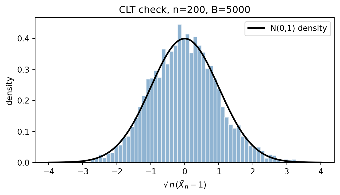
We sample $B$ independent batches, each of $n$ i.i.d. Exponential$(1)$ draws (mean $\mu = 1$, variance $\sigma^2 = 1$), form the standardized mean $\sqrt{n}(\bar{X}_n - 1)$, and compare its histogram to $\mathcal{N}(0, 1)$.
```{python}
#| label: fig-clt
#| fig-cap: "CLT for Exponential(1): standardized sample mean vs. standard normal density."
n, B = 200, 5000
samples = rng.exponential(scale=1.0, size=(B, n))
means = samples.mean(axis=1)
z = (means - 1.0) / (1.0 / np.sqrt(n))

fig, ax = plt.subplots(figsize=(6, 3.5))
ax.hist(z, bins=60, density=True, alpha=0.6, color="steelblue", edgecolor="white")
grid = np.linspace(-4, 4, 300)
ax.plot(grid, norm.pdf(grid), color="black", lw=2, label="N(0,1) density")
ax.set_xlabel(r"$\sqrt{n}(\bar X_n - 1)$")
ax.set_ylabel("density")
ax.set_title(f"CLT check, n={n}, B={B}")
ax.legend()
plt.tight_layout(); plt.show()
print(f"empirical mean={z.mean():.4f}, sd={z.std():.4f} (target 0, 1)")
```
Empirical mean is near zero and standard deviation near one, consistent with @eq-clt.
### Sample vs theoretical Gaussian CDF
We draw $N$ i.i.d. standard normals, compute the empirical CDF on a grid, and compare to $\Phi$.
```{python}
#| label: gaussian-cdf
N = 200_000
x = np.linspace(-3, 3, 13)
emp = rng.standard_normal(N)
sample_cdf = np.array([(emp <= xi).mean() for xi in x])
theo_cdf = norm.cdf(x)
diff = np.max(np.abs(sample_cdf - theo_cdf))
print(f"max |F_N - Phi|({N} draws) = {diff:.4f}")
```
The maximum absolute difference is small and scales as $O(1/\sqrt{N})$, the Dvoretzky-Kiefer-Wolfowitz rate.
### SVD reconstruction error
We build a random $80 \times 40$ matrix and reconstruct it from its rank-$k$ SVD truncation for several $k$. The relative Frobenius error is $\sqrt{\sum_{i > k} \sigma_i^2 / \sum_i \sigma_i^2}$ by Eckart-Young.
```{python}
#| label: svd-recon
A = rng.standard_normal((80, 40))
U, s, Vt = np.linalg.svd(A, full_matrices=False)
A_norm = np.linalg.norm(A, "fro")
for k in [5, 10, 20, 40]:
    Ak = U[:, :k] @ np.diag(s[:k]) @ Vt[:k, :]
    err_emp = np.linalg.norm(A - Ak, "fro") / A_norm
    err_theo = np.sqrt(np.sum(s[k:]**2)) / A_norm
    print(f"k={k:2d}  empirical={err_emp:.4f}  theoretical={err_theo:.4f}")
```
The empirical and theoretical errors agree to machine precision.
### KKT system for a toy QP
We solve
$$
\min_{\mathbf{x} \in \mathbb{R}^2} \tfrac{1}{2}\mathbf{x}^\top \mathbf{Q} \mathbf{x} + \mathbf{c}^\top \mathbf{x}
\quad \text{s.t.} \quad \mathbf{A}\mathbf{x} = \mathbf{b},
$$ {#eq-toyqp}
with $\mathbf{Q} = \begin{pmatrix} 4 & 1 \\ 1 & 3 \end{pmatrix}$, $\mathbf{c} = (-1, -2)^\top$, $\mathbf{A} = (1, 1)$, $\mathbf{b} = 1$. The KKT system is a single linear solve.
```{python}
#| label: toy-kkt
Q = np.array([[4., 1.], [1., 3.]])
c = np.array([-1., -2.])
Aeq = np.array([[1., 1.]])
beq = np.array([1.0])

KKT = np.block([[Q, Aeq.T],
                [Aeq, np.zeros((1, 1))]])
rhs = np.concatenate([-c, beq])
sol = np.linalg.solve(KKT, rhs)
x_star, lam = sol[:2], sol[2:]
primal_obj = 0.5 * x_star @ Q @ x_star + c @ x_star
print(f"x* = {x_star},  lambda = {lam},  f(x*) = {primal_obj:.4f}")
print(f"primal feasibility |Ax*-b| = {abs(Aeq @ x_star - beq)[0]:.2e}")
print(f"stationarity ||Qx*+c+A^T lambda|| = {np.linalg.norm(Q@x_star + c + Aeq.T@lam):.2e}")
```
Both KKT residuals are at machine precision, so $\mathbf{x}^*$ is the primal optimum and $\lambda$ is the equality multiplier.
### IRLS logistic regression from scratch
We simulate a logistic model with known coefficients, fit by IRLS using @eq-irls, and compare to `sklearn.linear_model.LogisticRegression` with no penalty. The sigmoid is evaluated through `creditutils.stable_sigmoid`, which uses the branchless overflow-safe form $\pi(\eta) = \mathbb{1}\{\eta \ge 0\}\,/(1+e^{-\eta}) + \mathbb{1}\{\eta < 0\}\,e^{\eta}/(1+e^{\eta})$ so the exponent argument is always non-positive. The naive form $1/(1+e^{-\eta})$ overflows once $|\eta|$ exceeds roughly 700 in float64, which is small relative to the scores produced by IRLS on poorly conditioned designs; using the stable form is a free correctness guard. See @sec-ch07-impl for the same routine inside the production scorecard fitter.
```{python}
#| label: irls-scratch
n, p = 500, 4
X = np.hstack([np.ones((n, 1)), rng.standard_normal((n, p))])
beta_true = np.array([0.2, 1.0, -0.5, 0.3, 0.0])
eta = X @ beta_true
prob = stable_sigmoid(eta)
y = (rng.uniform(size=n) < prob).astype(float)

def irls_logistic(X, y, max_iter=50, tol=1e-10):
    beta = np.zeros(X.shape[1])
    for it in range(max_iter):
        eta = X @ beta
        mu = stable_sigmoid(eta)
        W = np.clip(mu * (1.0 - mu), 1e-8, None)
        z = eta + (y - mu) / W
        XtW = X.T * W
        H = XtW @ X + 1e-10 * np.eye(X.shape[1])
        new_beta = np.linalg.solve(H, XtW @ z)
        if np.linalg.norm(new_beta - beta) < tol:
            beta = new_beta
            return beta, it + 1
        beta = new_beta
    return beta, max_iter

beta_hat, n_iter = irls_logistic(X, y)
skl = LogisticRegression(penalty=None, fit_intercept=False,
                         solver="lbfgs", max_iter=500).fit(X, y)
print(f"IRLS      beta = {beta_hat}  ({n_iter} iters)")
print(f"sklearn   beta = {skl.coef_.ravel()}")
print(f"max abs diff  = {np.max(np.abs(beta_hat - skl.coef_.ravel())):.2e}")
```
IRLS and scikit-learn agree to several decimals and recover the true coefficients up to sampling noise. The asymptotic variance at the MLE is the inverse Fisher information, which we can also compute from the final weights.
```{python}
#| label: fisher-info
mu = stable_sigmoid(X @ beta_hat)
W = mu * (1.0 - mu)
I_hat = (X.T * W) @ X
se = np.sqrt(np.diag(np.linalg.inv(I_hat)))
print("beta_hat:", beta_hat)
print("SE     :", se)
```
The standard errors come straight out of @eq-fisher and the MLE asymptotic normality in @eq-mle.
### Bootstrap confidence interval for AUC
We use the score $s(\mathbf{x}) = \mathbf{x}^\top \hat{\mathbf{\beta}}$ and compute a nonparametric percentile bootstrap 95% CI for the AUC.
```{python}
#| label: boot-auc
scores = X @ beta_hat
B = 1000
auc_b = np.empty(B)
for b in range(B):
    idx = rng.integers(0, n, n)
    auc_b[b] = roc_auc_score(y[idx], scores[idx])

auc_point = roc_auc_score(y, scores)
ci_lo, ci_hi = np.quantile(auc_b, [0.025, 0.975])
print(f"AUC point estimate = {auc_point:.4f}")
print(f"95% percentile CI  = [{ci_lo:.4f}, {ci_hi:.4f}] over B={B} resamples")
```
The CI is centered on the point estimate with width of the expected order. @sec-ch04 develops ROC/AUC inference in full, including the DeLong variance estimator and its comparison to the bootstrap.
```{python}
#| label: runtime-total
print(f"total runtime: {time.time() - t0:.2f} s")
```
## Further reading
For the probability and measure background, @billingsley1995probability remains the canonical graduate text; @casella2002statistical covers inference at the advanced undergraduate level and is a useful bridge for practitioners. Convex optimization is covered end to end in @boyd2004convex, with @nocedal2006numerical for numerical methods including IRLS and quasi-Newton. For linear algebra, @golub2013matrix and @trefethen1997numerical are the two books to own, with @horn2012matrix as the theoretical reference. Information theory is @cover1999elements. The bootstrap has @efron1993introduction as the accessible monograph and @efron1979bootstrap as the original. Asymptotic theory of the MLE, score tests, Wald, and LR is treated in @vandervaart1998asymptotic and @lehmann1998theory. Causal inference: @pearl2009causality for graphs and identification, @imbens2015causal for the potential outcomes program. Survival analysis: @klein2003survival. The GLM framework in general, and logistic regression by IRLS in particular, is covered in @mccullagh1989glm and @green1984iteratively.
## Takeaways
- Conditional expectation $\mathbb{E}[Y \mid \mathbf{X}]$ is the target of every classifier; everything else (calibration, ROC, costs) is a function of how well this object is estimated.
- SVD, spectral decomposition, Woodbury, and Schur complement cover most of the linear algebra moves used in the book.
- KKT conditions are the single most useful tool for understanding what a regularized estimator does at the optimum, including L1 sparsity.
- The logistic loss is binary cross-entropy is negative log-likelihood; IRLS is Newton's method on that loss.
- MLE, Fisher information, and the Delta method give asymptotic standard errors for almost any smooth transformation of regression coefficients, and the bootstrap backs them up without closed-form formulas.
- Ignorability, overlap, and SUTVA are the three assumptions to check before claiming any causal interpretation of a credit scoring model.