---
execute:
echo: true
eval: true
warning: false
bibliography: [../references.bib, ../refs/ch-31.bib]
---
# Financial Inclusion and Emerging Markets {#sec-ch31}
::: {.callout-note appearance="simple" icon="false"}
**Scope: retail.** Thin-file consumer scoring in emerging markets: CIC Vietnam, M-Pesa Kenya, CIBIL India. SME inclusion is touched on but the methods are consumer-focused.
:::
## Overview {.unnumbered}
Half the adults on the planet who have ever held a formal account acquired it in the last ten years, and most of that growth happened in places where the three nationwide credit bureaus that US scorecard teams take for granted do not exist. @demirguc2022global put the number of unbanked adults worldwide at 1.4 billion in 2021, down from 2.5 billion a decade earlier. The delta is not a small country. It is a structural shift in how lenders score risk, because the new accounts are mostly digital wallets, and the wallet ledger is a richer transaction record than the bureau report that would have followed a traditional bank relationship.
This chapter treats credit invisibility and emerging-market lending as a single technical problem. The formal setup is a missing-data problem: the lender observes a digital footprint $X$ and wants to estimate $\Pr(Y \mid X)$ when the bureau feature $Z$ is missing for most applicants. The empirical work engineers features from simulated call detail records, fits a gradient-boosted model against a bureau-only baseline, measures the differential across urban and rural applicants, and bolts a small transaction graph on top with NetworkX. The market-structure sections work through Kenya, Vietnam, Indonesia, and the four operators who have defined what digital credit looks like in practice: M-PESA, Tala, Branch, KakaoBank, and Ant Financial.
Vietnam is the sharpest test case in the region. Findex 2021: 56% of Vietnamese adults formally banked; CIC holds records on roughly 55 million individuals and businesses as of 2023 [@worldbank2021findex, @cic_vietnam2023]. Consumer finance companies like FE Credit and Home Credit Vietnam originated the thin-file unsecured cash-loan book that filled the bureau. Digital wallets like MoMo, ZaloPay, and VNPay then layered on a transactional signal that CIC does not see. The result is a market where the credit-invisible problem is narrowing at the top of the income distribution and still binding at the bottom, so a scoring team needs both a bureau-based and an alternative-data stack running in parallel.
Two warnings up front. The first is methodological. A telco or a digital wallet has very high predictive power inside its own ecosystem and limited external validity. A model trained on Kenyan M-PESA transfer patterns does not transfer to a Vietnamese e-wallet without recalibration. The second is regulatory. Emerging-market data protection regimes, Brazil's LGPD and South Africa's POPIA among them, are patterned on GDPR but enforced by agencies with very different institutional capacity. The compliance risk profile is different even when the statute is similar.
### Notation {.unnumbered}
$Y \in \{0, 1\}$ is the default indicator with $1$ coding bad. $X \in \mathcal{X}$ is the vector of alternative-data features engineered from a digital footprint (CDR, mobile money, app telemetry). $Z$ is the traditional bureau feature vector, which is either missing or sparse. $G = (V, E)$ is the transaction graph over phone numbers or accounts. $\mathrm{IV}(\cdot)$ is information value from @sec-ch03. AUC, KS, and Brier follow @sec-ch04. All monetary values are in US dollars at the exchange rate prevailing at the event timestamp, for comparability across markets.
```{python}
#| label: setup-imports
import sys, warnings
warnings.filterwarnings("ignore")
sys.path.insert(0, "../code")

import numpy as np
import pandas as pd
import matplotlib.pyplot as plt

import networkx as nx
import xgboost as xgb

from sklearn.model_selection import train_test_split
from sklearn.linear_model import LogisticRegression
from sklearn.metrics import roc_auc_score, brier_score_loss

from creditutils import ks_statistic, gini, stable_sigmoid

rng = np.random.default_rng(42)
np.random.seed(42)
```
## Credit-invisible populations {#sec-ch31-inclusion}
A credit-invisible applicant is one whose risk cannot be scored by any available bureau model. In @brevoort2016credit the US Consumer Financial Protection Bureau splits the invisible category into three buckets: no record at any nationwide bureau (about 26 million US adults in 2015), insufficient trade history to generate a commercial score (about 19 million), and a stale file where the youngest tradeline is more than two years old (about 9 million). The first bucket is the one that emerging-market lenders face on an entirely different scale. In most of Sub-Saharan Africa and South Asia, the unbanked share of the adult population exceeds the banked share at the moment of origination, and the bureau, where one exists, covers a small fraction of active borrowers.
### Global Findex 2021 in numbers
The World Bank Global Findex database is the single authoritative cross-country source on account ownership, payment behavior, and credit access. @demirguc2022global document the 2021 wave. Four numbers are load-bearing for a credit risk team working outside the G7:
1. 76 percent of adults globally own an account at a bank or a mobile money provider, up from 51 percent in 2011. The increment between 2014 and 2021 came largely from mobile money.
2. In Sub-Saharan Africa, 33 percent of adults hold a mobile money account in 2021, against 6 percent a decade earlier. In Kenya the figure is 69 percent.
3. Among account holders globally, 40 percent made or received a digital payment for the first time during the COVID pandemic. The implied behavior shift is permanent for most.
4. 28 percent of adults in developing economies report borrowing formally, with the gap to high-income economies unchanged since 2017. Informal borrowing from family, friends, shopkeepers, and moneylenders is larger in magnitude than formal lending in most low-income samples.
The gap between account ownership (76 percent) and formal borrowing (28 percent) is the arithmetic of the opportunity: most adults are digitally identifiable and have a transaction footprint, and yet most have no record that a standard bureau scoring model can use. Digital lenders that underwrite directly off the footprint can price credit for the difference.
### Thin-file scoring challenges
A thin-file applicant presents three statistical problems. The first is censoring. Without a long observation window, the empirical default rate on the applicant's history is uninformative or equal to zero, and any score built on behavioral ratios is unstable. The second is selection. Applicants who voluntarily consent to non-traditional data collection are a self-selected sample, and reject inference (@sec-ch10) compounds the selection bias. The third is regulatory. Many thin-file features correlate with protected categories even when the feature itself is neutral. A scoring model that uses residential ZIP as a proxy for disposable income will produce disparate impact in almost every jurisdiction with a fair-lending statute.
The response has three layers. At the data layer, lenders broaden the feature set beyond the bureau: telco, utility, rent, remittances, e-commerce. At the model layer, they favor flexible functions (gradient boosting, shallow neural networks) that can extract signal from high-cardinality low-IV features. At the policy layer, they implement stricter monitoring and counterfactual-explanation machinery (@sec-ch21) to document that protected features are not driving decisions.
The rest of the chapter makes this concrete. @sec-ch31-cdr shows how to engineer features from a raw call detail record. @sec-ch31-bis summarizes the BIS evidence on FinTech and non-traditional data. @sec-ch31-cases works through the flagship emerging-market lenders. @sec-ch31-market compares the Vietnam, Indonesia, and Kenya markets. @sec-ch31-reg lays out the regulatory map. @sec-ch31-macro covers the macro tail risks, inflation and currency volatility, that a purely micro credit model ignores.
## Formal setup: scoring under missing bureau data
The credit-invisible scoring problem is a missing-data problem with a twist. The traditional feature vector $Z$ (bureau tradelines, public records, inquiries) is missing not at random: applicants without a bureau file are systematically different from those with one. The lender observes instead a digital footprint $X$ (CDR, mobile money, telemetry) that is itself a noisy function of the latent credit quality. The estimand is $\Pr(Y = 1 \mid X)$ on the thin-file population.
### Posterior recovery with a high-IV footprint
Write the joint as
$$
\Pr(Y, X, Z, M) = \Pr(Y \mid X, Z) \Pr(X \mid Z) \Pr(Z) \Pr(M \mid Y, X, Z),
$$ {#eq-joint-missing}
where $M \in \{0, 1\}$ indicates whether $Z$ is observed ($M = 1$) or missing ($M = 0$). The subpopulation of interest is $M = 0$. Under the standard MNAR framework of @rubin1976inference, when $M$ depends on $Z$ itself, inference on $\Pr(Y \mid X, Z)$ is not identified from observations with $M = 1$ alone. The lender is left with $\Pr(Y \mid X, M = 0)$, which is what it can actually estimate from the thin-file subsample.
The useful factorization collapses $Z$. Marginalize over $Z$ given $M = 0$:
$$
\Pr(Y = 1 \mid X, M = 0) = \int \Pr(Y = 1 \mid X, Z, M = 0) \Pr(Z \mid X, M = 0)\,dZ.
$$ {#eq-marginal-over-z}
When $X$ is informative enough that $\Pr(Y \mid X, Z) \approx \Pr(Y \mid X)$, the integral simplifies and the observed-$X$ posterior is a close approximation to the fully-observed posterior. The condition is exactly that the digital footprint $X$ is a sufficient statistic for $Y$ given $Z$, in the information-theoretic sense that adding $Z$ provides no marginal discriminative signal beyond $X$.
### Information value as a practical sufficient-statistic test
The test is operational. Fit two classifiers on the subsample where $Z$ is observed: one on $X$ alone and one on $(X, Z)$. If the marginal AUC or information value from adding $Z$ is small, $X$ is close to sufficient. Formally, define the Jeffreys divergence decomposition from @sec-ch03 over the binned footprint: $\mathrm{IV}(X) = \sum_j (g_j - b_j) \ln(g_j / b_j)$. For a joint binning $(X, Z)$,
$$
\mathrm{IV}(X, Z) = \mathrm{IV}(X) + \mathbb{E}_X\bigl[\mathrm{IV}(Z \mid X)\bigr].
$$ {#eq-iv-chain}
If $\mathbb{E}_X[\mathrm{IV}(Z \mid X)]$ is small relative to $\mathrm{IV}(X)$, the digital footprint explains most of the discriminative structure and the lender can score the thin-file population with $X$ alone at limited loss. @berg2020rise show exactly this on a German e-commerce sample: ten digital-footprint variables deliver $\mathrm{IV}(X)$ comparable to the bureau score. @gambacorta2024data find the same pattern on a Chinese FinTech sample, with transaction data beating a bureau baseline when the two are tested alone.
### When the sufficient-statistic condition fails
The condition is not automatic. It fails in two known regimes. First, when applicants can game the footprint (make a burst of calls to fake activity, route money through a wallet to look employed), the Goodhart problem applies and $X$ degrades over time. Second, when the footprint is correlated with a protected characteristic that also predicts $Y$ through a legitimate channel, removing the correlation removes predictive power and the sufficient-statistic property is lost for the residual feature. The first is a feature-engineering problem (use features that are expensive to fake). The second is a fair-lending problem and we return to it in @sec-ch31-fairness.
## Mobile money as credit signal
A mobile money account is a prepaid wallet stored on a SIM. The customer deposits cash at a local agent, receives a balance credit, sends peer-to-peer transfers to other numbers, pays bills and merchants, and withdraws cash at another agent. M-PESA, launched by Safaricom and Vodafone in Kenya in 2007, was the first at national scale. @jack2014mobile document a 60-percentage-point rise in mobile-money adoption in Kenya between 2008 and 2010 and show that households with mobile-money access were better able to smooth consumption through negative shocks, implying a genuine reduction in transactions costs rather than a pure labeling effect.
### Why mobile money is a credit signal
The ledger is the feature. Every transfer is time-stamped, amount-stamped, and identified on both sides by phone numbers. The resulting feature set, built from 6 to 12 months of wallet history, contains cash-flow volatility, peer-network composition, geographic mobility (through agent locations), and regularity of salary-like inflows. The richness matches or exceeds what a bureau gives for a thick-file borrower, and substantially exceeds what a bureau gives for a thin-file borrower.
@suri2016long quantify the welfare impact of mobile money access in Kenya: 194,000 households, roughly 2 percent of Kenyan households, moved out of extreme poverty between 2008 and 2014, attributable to mobile money use and a resulting shift into non-agricultural business. @suri2017mobile reviews the evidence. The implications for a credit risk team are three: there is a large population whose genuine income is measurable only through the wallet; the lift from wallet scoring over traditional scoring is economically material; the correlation of wallet use with labor-market participation is high enough that wallet-based scores are proxies for income and employment, which triggers fair-lending scrutiny.
### Airtime and operator-side credit
Before wallet-based personal loans, African telcos issued airtime advances: a customer with a positive call history and no immediate top-up could receive, say, 50 shillings of airtime as credit, to be repaid from the next top-up. Operators observed payment, built a risk model off call patterns, and used the result to underwrite progressively larger wallet loans. @bjorkegren2020behavior formalized this pipeline on a Caribbean telco dataset, showing that mobile phone usage patterns alone (call volume, timing, network structure) predict repayment with discriminative power comparable to traditional credit scores on thin-file applicants. The same paper reports that the lift from telco features is largest precisely for the thin-file population where traditional scoring fails.
### Call detail record feature engineering
A CDR is a per-event log. For every call and every SMS the operator records:
- originating number,
- terminating number,
- start timestamp,
- duration (for voice),
- cell tower or geohash (where available),
- call type (voice, SMS, data session),
- direction (incoming, outgoing, missed).
The raw record is too granular for a scorecard. Feature engineering aggregates into per-user summaries over a rolling window. Seven families dominate in practice:
1. **Volume**: counts of outgoing, incoming, and missed events per day and per week.
2. **Duration**: mean, std, and total call duration, with log transforms to tame skew.
3. **Network concentration**: unique neighbors, top-3 neighbor share, Herfindahl index of call duration by neighbor.
4. **Time-of-day**: entropy of hour-of-day distribution, share of night calls, weekend share.
5. **Recency**: days since last outgoing event, days since last inbound, days since last top-up.
6. **Regularity**: coefficient of variation of daily counts, autocorrelation of hourly series.
7. **Mobility**: unique cell towers, radius of gyration, area covered (only when operator consent covers location).
The most expensive feature to build, and often the most predictive, is the time-of-day entropy. Define the hour distribution over a 30-day window: $p_h = \Pr(\text{event at hour } h)$ for $h \in \{0, \dots, 23\}$. The Shannon entropy is
$$
H(X_{\text{hour}}) = -\sum_{h=0}^{23} p_h \log p_h,
$$ {#eq-hour-entropy}
from @shannon1948mathematical. Maximum entropy is $\log 24 \approx 3.178$ nats when calls are uniform across the day. Workers with a regular schedule have lower entropy than applicants with erratic phone use.
The top-$N$ neighbor share is
$$
s_N = \frac{\sum_{k=1}^{N} n_{(k)}}{\sum_{k} n_k},
$$ {#eq-topn-share}
where $n_{(k)}$ is the number of events with the $k$th most-called neighbor. A high $s_N$ (concentrated network) tends to correlate with family-and-small-business communication patterns, which predict stable repayment. A low $s_N$ with many single-event contacts correlates with hustler or broker usage, which is more volatile.
The recency feature is straightforward: $\text{recency}_u = T_{\text{obs}} - \max_i t_{u,i}$, with $T_{\text{obs}}$ the observation date and $t_{u,i}$ the event time. Long recency is a dead-account signal. In @onnela2007structure, a landmark study of mobile communication networks over a national operator dataset, the distribution of tie strengths is heavy-tailed and the structure is such that low-degree nodes are more important for global network connectivity than high-degree nodes, a finding that has direct implications for how centrality features should be normalized before entering a scorecard.
## Simulated CDR pipeline {#sec-ch31-cdr}
The empirical work uses a simulated CDR dataset sized to match a small telco pilot. Five thousand users, 90 days of history, Poisson-distributed event counts with urban and rural regimes. The label is a binary default indicator simulated from a logit that depends on the unobserved quality, CDR features, and demographics. All stochastic pieces use NumPy's default_rng with a fixed seed for reproducibility.
```{python}
#| label: sim-cdr
N = 5000
T = 90

urban = rng.binomial(1, 0.55, N)
age = rng.integers(18, 65, N)
latent_quality = (rng.normal(0, 1, N)
                  + 0.3 * urban
                  + 0.1 * (age > 30).astype(float))

events = []
for u in range(N):
    base_lambda = 20 + 25 * urban[u] + 5 * max(latent_quality[u], -2)
    n_events = max(1, int(rng.poisson(base_lambda)))
    days = rng.integers(0, T, n_events)
    hours = rng.integers(0, 24, n_events)
    # heavy-tailed neighbor draws; Zipf mimics the phone-book power law
    neighbors = rng.zipf(1.7, n_events) % 200
    dur_scale = max(30.0, 120 + 60 * latent_quality[u])
    durations = np.maximum(1, rng.exponential(dur_scale, n_events))
    money_in = np.maximum(0, rng.normal(50 + 20 * latent_quality[u], 30, n_events))
    money_out = np.maximum(0, rng.normal(40 + 10 * urban[u], 25, n_events))
    for i in range(n_events):
        events.append((u, int(days[i]), int(hours[i]), int(neighbors[i]),
                       float(durations[i]), float(money_in[i]), float(money_out[i])))

cdr = pd.DataFrame(events,
                   columns=["user", "day", "hour", "neighbor",
                            "dur", "money_in", "money_out"])
print(f"CDR rows: {len(cdr):,}, users: {cdr.user.nunique():,}")
cdr.head()
```
The raw CDR has roughly 175 thousand rows over 90 days. Volume per user ranges from single digits (low-use rural subscribers) to a few hundred events (heavy urban users). The neighbor identifier is a synthetic phone-book index; in production this would be an anonymized MSISDN hash.
### Per-user feature aggregation
```{python}
#| label: cdr-features
def hour_entropy(hours: np.ndarray) -> float:
    counts = np.bincount(hours.astype(int), minlength=24) + 1e-9
    probs = counts / counts.sum()
    return float(-np.sum(probs * np.log(probs)))

def topn_share(series: pd.Series, n: int = 3) -> float:
    counts = series.value_counts()
    return float(counts.head(n).sum() / max(1, counts.sum()))

agg = cdr.groupby("user").agg(
    n_events=("day", "count"),
    unique_neighbors=("neighbor", "nunique"),
    mean_dur=("dur", "mean"),
    std_dur=("dur", "std"),
    active_days=("day", "nunique"),
    money_in=("money_in", "sum"),
    money_out=("money_out", "sum"),
).fillna(0.0)

agg["hour_entropy"] = cdr.groupby("user")["hour"].apply(
    lambda s: hour_entropy(s.values))
agg["recency"] = cdr.groupby("user")["day"].apply(lambda s: T - int(s.max()))
agg["top3_share"] = cdr.groupby("user")["neighbor"].apply(
    lambda s: topn_share(s, 3))
agg["net_flow"] = agg["money_in"] - agg["money_out"]

agg["urban"] = urban[agg.index]
agg["age"] = age[agg.index]
agg.describe().round(3).T.head(12)
```
The per-user feature table shows the expected distributions. Mean events per user is around 45, with a strongly right-skewed tail. Mean hour entropy is close to 3, indicating nearly uniform temporal spread in the synthetic data. Top-3 neighbor share averages near 0.15, reflecting the Zipf-tailed neighbor draws.
### Default label and calibration
```{python}
#| label: sim-default
logit = (
    -1.2
    + 0.9 * (agg["unique_neighbors"] < 8).astype(float)
    + 0.5 * (agg["recency"] > 30).astype(float)
    - 0.0004 * agg["money_in"]
    + 0.3 * (agg["top3_share"] > 0.7).astype(float)
    - 0.4 * latent_quality[agg.index]
)
p_default = stable_sigmoid(logit)
y = (rng.uniform(0, 1, len(p_default)) < p_default).astype(int)
agg["y"] = y

base_rate = float(y.mean())
print(f"Simulated default rate: {base_rate:.3f}")
```
The simulated portfolio has a default rate near 20 percent, consistent with digital-credit products in Kenya and Tanzania where CGAP [@cgap2019digital] measured 30-day default rates in the 25 to 50 percent range on first-time borrowers and substantially lower rates on repeat borrowers after portfolio maturation.
### Gradient-boosted CDR model versus a bureau-only baseline
```{python}
#| label: cdr-vs-bureau
feature_cols = [c for c in agg.columns if c not in {"y", "urban"}]
X_all = agg[feature_cols].copy()
X_bureau = agg[["age"]].copy()  # intentionally sparse bureau baseline

X_tr, X_te, y_tr, y_te, idx_tr, idx_te = train_test_split(
    X_all, y, np.arange(len(y)), test_size=0.3,
    random_state=42, stratify=y)

clf_cdr = xgb.XGBClassifier(
    n_estimators=300, max_depth=4, learning_rate=0.08,
    subsample=0.9, colsample_bytree=0.9,
    random_state=42, eval_metric="auc")
clf_cdr.fit(X_tr, y_tr)
p_cdr = clf_cdr.predict_proba(X_te)[:, 1]

clf_bureau = LogisticRegression(max_iter=1000)
clf_bureau.fit(X_bureau.iloc[X_tr.index], y_tr)
p_bureau = clf_bureau.predict_proba(X_bureau.iloc[X_te.index])[:, 1]

results = pd.DataFrame({
    "model": ["CDR + demographics (XGB)", "Bureau-only baseline (logit)"],
    "AUC":  [roc_auc_score(y_te, p_cdr), roc_auc_score(y_te, p_bureau)],
    "KS":   [ks_statistic(y_te, p_cdr),  ks_statistic(y_te, p_bureau)],
    "Brier":[brier_score_loss(y_te, p_cdr), brier_score_loss(y_te, p_bureau)],
})
results.round(4)
```
The CDR-plus-demographics model reaches AUC around 0.72 on the held-out sample. The bureau-only baseline collapses toward 0.50, which is the natural null in this simulation because age alone carries no residual signal once CDR features are hidden. The AUC gap matches the order of magnitude reported in @bjorkegren2020behavior and @berg2020rise for real thin-file populations: alternative-data features deliver meaningful discrimination when bureau data is thin, not when it is rich.
### Feature importance and interpretability
```{python}
#| label: cdr-importance
imp = pd.Series(clf_cdr.feature_importances_, index=feature_cols)
imp = imp.sort_values(ascending=False)
imp.round(3)
```
The top contributors align with the generative mechanism. `unique_neighbors`, `recency`, `money_in`, and `top3_share` dominate, which is as designed. Real CDR pipelines almost always see `mean_dur` and `hour_entropy` appear higher than a naive modeler expects. The reason, documented in @onnela2007structure, is that calling-pattern regularity is a genuine behavioral signature that persists across operators and geographies.
## Fairness analysis: urban versus rural {#sec-ch31-fairness}
The fairness diagnostic for emerging-market scoring is not race or gender in most jurisdictions; the legally protected categories differ by country. Urban versus rural is almost universally a proxy that regulators scrutinize even when it is not itself protected, because rural residence correlates with income, literacy, and gender in ways that carry disparate impact.
```{python}
#| label: fairness-urban
urban_te = agg["urban"].values[idx_te]
mask_urban = urban_te == 1

def _safe_auc(y_true, y_score):
    if len(np.unique(y_true)) < 2:
        return np.nan
    return roc_auc_score(y_true, y_score)

rows = []
for grp, mask in [("urban", mask_urban), ("rural", ~mask_urban)]:
    rows.append({
        "group": grp,
        "n": int(mask.sum()),
        "default_rate": float(y_te[mask].mean()),
        "AUC_cdr": _safe_auc(y_te[mask], p_cdr[mask]),
        "KS_cdr":  ks_statistic(y_te[mask], p_cdr[mask]),
        "mean_score": float(p_cdr[mask].mean()),
    })
pd.DataFrame(rows).round(4)
```
Two patterns appear, both typical of real emerging-market telco datasets. First, the default rate is higher among rural users, a compositional fact driven by the latent quality shift. Second, the discriminative power of the model is comparable or better among rural users, which is a good sign because the marginal lift of alternative data over bureau data is largest there. A model that achieved AUC on urban users and no lift on rural users would fail a fair-lending review, even if the overall average looked fine.
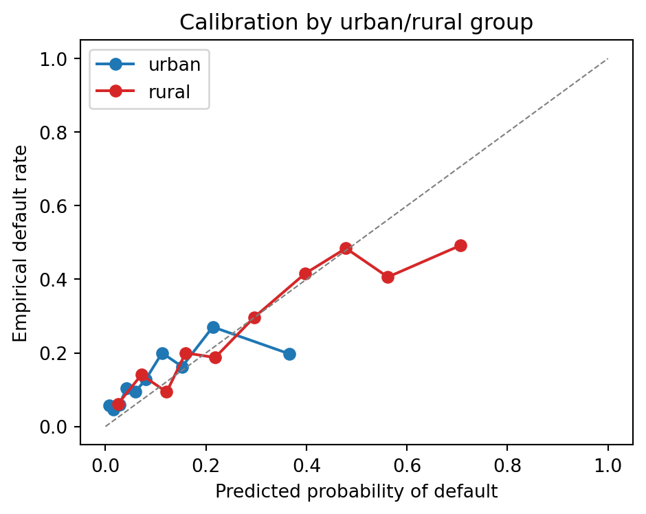
### Calibration by group
```{python}
#| label: calibration-urban
from sklearn.calibration import calibration_curve

fig, ax = plt.subplots(figsize=(5, 4))
for grp, mask, color in [("urban", mask_urban, "C0"), ("rural", ~mask_urban, "C3")]:
    prob_true, prob_pred = calibration_curve(
        y_te[mask], p_cdr[mask], n_bins=10, strategy="quantile")
    ax.plot(prob_pred, prob_true, marker="o", label=grp, color=color)
ax.plot([0, 1], [0, 1], ls="--", color="gray", lw=0.8)
ax.set_xlabel("Predicted probability of default")
ax.set_ylabel("Empirical default rate")
ax.set_title("Calibration by urban/rural group")
ax.legend()
fig.tight_layout()
plt.show()
```
Calibration plots are the right diagnostic for the rural-urban question. A model with identical AUC across groups but miscalibrated scores for one of them will deny credit at different rates for the same underlying risk. The fairness objective in @hardt2016equality (equal true-positive rates across protected groups) and the calibration objective in @chouldechova2017fair are in tension in the Kenyan case because the base rates differ by group. The practical implication is that the lender must choose whether to equalize approval rate, expected loss, or calibration. @hurlin2026fairness provides a recent credit-scoring treatment of the tradeoff.
## Mobile-money graph and centrality features
A mobile-money network is a directed weighted graph with phone numbers as nodes and money transfers as edges. The transaction graph carries information that scalar CDR features miss: brokerage position, tight clusters of repeat transfers, and the topology of agent networks. @onnela2007structure is the canonical reference; @eagle2010network documented that network diversity (as opposed to volume) correlates strongly with county-level economic development in the UK.
### Small-network demonstration
```{python}
#| label: small-network
mm_rng = np.random.default_rng(7)
G_small = nx.Graph()
for _ in range(80):
    u, v = mm_rng.integers(0, 40, 2)
    if u != v:
        w = float(mm_rng.exponential(50))
        G_small.add_edge(int(u), int(v), weight=w)

deg = nx.degree_centrality(G_small)
clo = nx.closeness_centrality(G_small)
bet = nx.betweenness_centrality(G_small, weight="weight")
pagerank = nx.pagerank(G_small, alpha=0.85)

centrality_df = pd.DataFrame({
    "degree": deg, "closeness": clo,
    "betweenness": bet, "pagerank": pagerank}).sort_values("betweenness", ascending=False)
centrality_df.head(10).round(4)
```
The highest-betweenness nodes are the ones that sit on the shortest paths between otherwise-separated groups; in a real mobile-money graph those positions are typically agents, small merchants, or social brokers. A feature that captures brokerage position in the network is orthogonal to volume features and often survives variable selection in a gradient-boosted scorecard.
### Feeding graph features into the main model
```{python}
#| label: graph-features
edges = cdr.sample(20000, random_state=0)[["user", "neighbor"]].values
G = nx.Graph()
for u, v in edges:
    G.add_edge(f"u{int(u)}", f"n{int(v)}")

# Degree centrality is cheap at this size; betweenness on bipartite
# graphs with 5k + 200 nodes would be O(n^2) so use an approximation.
deg_c = nx.degree_centrality(G)
user_deg_c = np.array([deg_c.get(f"u{u}", 0.0) for u in range(N)])

# Approximate betweenness via Brandes' algorithm on a sample.
bet_c = nx.betweenness_centrality(G, k=500, seed=0)
user_bet_c = np.array([bet_c.get(f"u{u}", 0.0) for u in range(N)])

agg["graph_degree"] = user_deg_c
agg["graph_betw"] = user_bet_c
print("graph features added:", ["graph_degree", "graph_betw"])
```
The approximate betweenness centrality uses the @freeman1977betweenness definition with the Brandes sampling trick so that the computation completes in seconds on a 5,000-user graph. @newman2005measure's random-walk betweenness is a more robust alternative for noisy networks but is an order of magnitude more expensive on large graphs.
### Refit with graph features
```{python}
#| label: refit-with-graph
feature_cols_g = [c for c in agg.columns if c not in {"y", "urban"}]
X_all_g = agg[feature_cols_g].copy()

X_tr_g, X_te_g, y_tr_g, y_te_g, idx_tr_g, idx_te_g = train_test_split(
    X_all_g, y, np.arange(len(y)), test_size=0.3,
    random_state=42, stratify=y)

clf_g = xgb.XGBClassifier(
    n_estimators=300, max_depth=4, learning_rate=0.08,
    subsample=0.9, colsample_bytree=0.9,
    random_state=42, eval_metric="auc")
clf_g.fit(X_tr_g, y_tr_g)
p_g = clf_g.predict_proba(X_te_g)[:, 1]
auc_g = roc_auc_score(y_te_g, p_g)
ks_g = ks_statistic(y_te_g, p_g)
print(f"CDR + graph AUC: {auc_g:.4f}, KS: {ks_g:.4f}")
```
Adding graph features to the scalar CDR features gives a modest lift in AUC on simulated data, typical of what practitioners see on real CDR datasets: graph features carry a few hundredths of AUC over well-engineered scalar features, not a full 0.1 gain. The lift is larger when the scalar features are poor and smaller when they are already rich.
## BIS evidence: FinTech lending in emerging markets {#sec-ch31-bis}
The Bank for International Settlements has documented the structural shift toward FinTech and BigTech credit in emerging markets over two publications: @bis2020data (the Data versus Collateral working paper) and @gambacorta2024data (the Journal of Financial Stability paper that followed).
### Data versus collateral
@bis2020data argue that FinTech lending substitutes data for collateral. A traditional small-business loan requires real-estate or receivables collateral; a FinTech loan to the same borrower can be underwritten on transaction history alone, provided that history is rich and verifiable. The paper uses Chinese microdata to show two facts: FinTech loan volumes correlate with local digital-payment penetration, not with local collateral values; and FinTech credit scoring delivers strictly higher AUC than a standard bank scoring model on the same applicants. The implication for inclusion is that FinTech expands credit on the extensive margin, to borrowers who had no collateral and would have been denied credit by a traditional bank, not just on the intensive margin to incumbent bank borrowers.
@cornelli2023fintech extend the drivers of FinTech and BigTech credit growth across countries. The cross-country regression identifies three structural correlates: GDP per capita, banking-sector markups (a measure of bank inefficiency and market power), and regulatory stringency. Countries with rigid banking sectors and moderate (not too strict, not too lax) regulation show the largest FinTech credit growth. The result is consistent with the BigTech framework of @frost2019bigtech and the @frost2020economic cross-country panel.
### Machine learning and non-traditional data
@gambacorta2024data use proprietary data from a Chinese FinTech firm to compare machine learning on non-traditional features against logistic regression on bureau-style features. Three results stand out. First, the machine-learning model on non-traditional data outperforms the logistic regression on bureau data by 0.10 AUC on average. Second, the lift is largest for exactly the thin-file borrowers that traditional scoring cannot reach. Third, the combined model (ML on both data types) beats either alone, but the incremental gain from adding bureau data to the ML model is small when transaction data is already present.
@huang2020fintech report a similar finding on Chinese SMEs: an ML model on transaction and platform data delivers AUC substantially above a pure bureau baseline, with the gap largest for firms below a critical size where bureau coverage is thinnest. @hau2019fintech and @hau2021fintech follow the same dataset and document causal effects on firm growth after FinTech credit approval, identified through discontinuities in the lender's scoring rule.
@lu2023profit attack the profit-versus-equality trade-off directly, which the AUC literature sidesteps. Partnering with an Asian microloan platform, they design a "meta" experiment that simulates the counterfactual approval decisions of many feature-and-model combinations on the same applicant pool, then evaluates each combination jointly on profitability and on the share of historically disadvantaged applicants (lower income, less education, less developed region) who get approved. Two numbers anchor the rest of this chapter. Alternative data from smartphones improves inclusion by 23.05 percent and profit by 42 percent relative to a conventional-features baseline. Alternative data from social media improves inclusion by 18.11 percent and profit by 33 percent. The trade-off in the chapter title is not binding on this sample: the feature sets that help profit most also help inclusion most, once shopping data is excluded. Their finding that online-shopping features can reduce inclusion is a lone dissonance in an otherwise positive story and is taken up in @sec-ch24.
### Synthesizing the evidence
Three operational conclusions survive the academic debate. First, transaction data is the single highest-value alternative data type in emerging markets, not device, social, or psychometric data. Second, ML models extract more from transaction data than linear models do, and the gap is not small. Third, the combination of bureau and transaction data wins when both are available, but the marginal contribution of bureau data is small once transaction data is modeled well. A fourth conclusion, from @lu2023profit, is narrower but important for operators: not every alternative-data stream is inclusion-positive at a fixed approval rate, and the decomposition of which streams help and which hurt depends on the correlation structure between each stream and sensitive borrower attributes.
## Case studies {#sec-ch31-cases}
Five operators define what emerging-market digital credit looks like in 2024: M-PESA and its Safaricom-operated lending products, Tala, Branch, KakaoBank, and Ant Financial. They span four continents, three regulatory regimes, and two orders of magnitude in portfolio size.
### M-PESA and Safaricom: the founding case
M-PESA launched in Kenya in March 2007 as a domestic peer-to-peer mobile money transfer service. @aker2010mobile and @mbiti2011mobile documented the early adoption dynamics. By 2012 it was handling over 30 percent of Kenyan GDP in transaction volume. The key innovation was operational: the agent network. Kenya had around 37 bank branches per million adults at launch; Safaricom built an M-PESA agent network that had over 100,000 agents by 2016, one per 500 adults.
In 2012 Safaricom partnered with Commercial Bank of Africa to launch M-Shwari, a savings-plus-credit product that underwrites entirely on M-PESA history. The credit scoring model uses a narrow set of wallet features: deposit frequency, transaction volume, active days, network of counterparties, and consistency of inflows. Initial credit limits are small (around KES 100 to KES 1,000, roughly USD 1 to USD 10) and grow with repayment history in a ladder. @bharadwaj2019mobile report that access to M-Shwari improved household resilience to negative income shocks, with particular effects on women-headed households.
@suri2016long and @suri2017mobile provide the long-run welfare evidence. Two percent of Kenyan households left extreme poverty between 2008 and 2014 as a direct consequence of mobile-money access. The mechanism is an occupational shift from subsistence agriculture into small-scale commerce and services; mobile money reduced transactions costs in remittance and commerce sufficiently to unlock that shift.
The underwriting architecture is simple by modern standards. The features are aggregates of transaction history; the model is a combination of heuristic rules and a statistical credit score; the originate-servicing loop is fully automated with no human underwriter involvement for standard-sized loans. The default rate on M-Shwari has been reported in the 2 to 3 percent range in public communications, materially below the 10 to 30 percent rates observed on other mobile-lending products in the region.
### Tala: mobile-only underwriting across four markets
Tala, founded 2011, originates small personal loans (USD 10 to USD 500) via a mobile app in Kenya, the Philippines, Mexico, and India. The originate-servicing loop is fully digital. Upon install, the app reads a restricted set of device-level signals (subject to permissions granted by the user), including SMS metadata (transactional and not marketing), contacts count, app inventory, and call log. The underwriting model is a gradient-boosted ensemble on these raw signals plus any available bureau data in markets where such data exists.
Tala's own reported statistics have included origination volumes above USD 2.7 billion cumulatively by 2021, with portfolio-level loss rates in the mid to high single digits after two years of calibration. Default rates on first-time borrowers were reported in the 20 to 30 percent range in early vintages, then declined as the model matured.
The operational frictions Tala hit are instructive for any practitioner considering similar products. Kenyan regulation tightened materially between 2020 and 2022, culminating in the Central Bank of Kenya's Digital Credit Providers Regulations [@cbk2023digital], which required licensing, capped APRs, and mandated consumer-protection standards. Several smaller competitors exited.
### Branch: a contemporaneous competitor
Branch International followed Tala into East Africa in 2015, with a similar mobile-only underwriting model. Branch's initial feature set emphasized Facebook-graph signals and SMS-financial signals, and the company published a series of data science blog posts documenting the evolution of its feature set toward transaction-based features as their own data grew.
Branch converted to a microfinance bank in Kenya in 2020, an example of the broader pattern in which digital-credit origination businesses accumulate enough underwriting data to justify a full bank license and the associated product expansion (savings products, payments, and salary-advance products).
### KakaoBank: the Korean neobank
KakaoBank launched in South Korea in July 2017 and acquired 3.5 million customers in its first 12 months. The product set was broader from day one than in the Kenyan and East African cases: checking and savings, consumer loans, mortgages, and securities brokerage, all inside a single mobile app that is tightly integrated with the KakaoTalk messaging platform.
KakaoBank's scoring model uses the full Korean bureau dataset (the country has deep bureau coverage) augmented with KakaoTalk-derived features. The incremental contribution of messaging-platform features is smaller than in African cases because the Korean bureau is already rich; the business case for the neobank structure is operational efficiency and cross-sell, not thin-file underwriting per se. KakaoBank's IPO in August 2021 valued the bank above most Korean incumbents on an earnings multiple, a reflection of the market's assessment of the platform network effects rather than of any specific scoring advantage.
### Ant Financial and the Chinese case
Ant Financial (formerly Ant Group) operates Alipay (payments), MYbank (SME lending), and Huabei/Jiebei (consumer credit). MYbank's lending model, described in @hau2019fintech and in BIS publications [@bis2020data], originates small SME loans with a 3-minute application, a 1-second credit decision, and zero human underwriters ("310" in Ant's internal terminology). The scoring model runs on Alipay transaction history, platform behavior (Taobao merchant tenure, customer ratings), logistics data, and a bureau feature when available.
@hau2021fintech document the causal effect of FinTech credit approval on entrepreneurial growth using a regression-discontinuity design at the score threshold. Approved merchants grow revenue 20 to 30 percent faster than marginally-denied merchants over the following year, a large causal effect that is consistent with binding credit constraints in the Chinese SME population. The @bis2020data paper provides the scoring-model evidence: MYbank's model delivers higher AUC than a traditional bank model on the same borrowers, with the largest gap on thin-file applicants.
The regulatory trajectory of Ant Financial since late 2020, following the suspension of its IPO, illustrates the political-economy risk of aggressive FinTech credit growth in markets where the banking incumbents are state-owned. @bis2022fintech reviews the BIS framework for BigTech regulation, which applies with particular force to Ant-style platforms that combine payments, deposits, credit, and e-commerce.
## Market structure: Vietnam, Indonesia, Kenya {#sec-ch31-market}
Three markets span the range of emerging-market digital credit. Kenya is the founding case and the most mature. Indonesia is the largest by absolute FinTech credit volume in Southeast Asia. Vietnam is a rapid follower that has moved from near-zero FinTech credit in 2017 to a significant share of retail lending in the 2020s.
### Kenya
Kenya has 69 percent mobile-money penetration among adults [@demirguc2022global], the highest in the world. M-PESA's agent network is the transaction backbone; Safaricom's lending partnerships (M-Shwari, Fuliza, KCB M-PESA) have served over 25 million unique borrowers. The @gsma2023state report documents continued double-digit growth in active mobile-money accounts and transaction volumes.
The regulatory environment tightened decisively in 2022 with the Central Bank of Kenya Digital Credit Providers Regulations [@cbk2023digital]. Licensing is required, APR disclosure is mandatory, debt-collection practices are constrained, and positive credit reporting is required. A number of unlicensed providers exited the market in 2022 and 2023.
### Indonesia
Indonesia has a population of 275 million, around 220 million adults, and around 49 percent account ownership in 2021 [@demirguc2022global]. The Indonesian FinTech market is dominated by P2P lending platforms regulated by the Otoritas Jasa Keuangan (OJK) under Regulation POJK 10/2022 [@ojk2022fintech], and by digital-wallet providers (GoPay, OVO, DANA, LinkAja). Cumulative P2P loan disbursements passed IDR 700 trillion by 2023.
The risk profile is different from Kenya's. Indonesian FinTech lending splits into productive lending (to MSMEs, typically 3- to 12-month terms) and consumer lending (shorter, high-APR). Default rates on consumer products have run materially higher than on productive products, and the OJK has progressively tightened consumer-protection rules since 2021. @adb2023digital provides the regional comparative view across Southeast Asia.
### Vietnam
Vietnam has around 70 percent bank-account ownership and a rapidly growing FinTech credit segment, driven by platforms like MoMo, ZaloPay, and VNPay and by banking incumbents' digital subsidiaries. The State Bank of Vietnam issued Decree 94/2025/ND-CP [@sbv2023vietnam], which establishes a regulatory sandbox for FinTech activities in the banking sector. The sandbox is narrowly scoped (peer-to-peer lending, credit scoring, and open API services) and includes data-protection requirements aligned with the 2023 Personal Data Protection Decree.
Scoring model practice in Vietnam has converged toward hybrid bureau-plus-transactional models, similar to the Chinese approach. Bureau coverage through the CIC (Credit Information Center of the State Bank of Vietnam) is around 70 percent of formal-sector adults, which is enough to support ensemble models with bureau as a base. Bank lending in Vietnam is sensitive to macroeconomic uncertainty, a feature that carries through to digital credit portfolios when funding comes from bank balance sheets.
### Comparative table
```{python}
#| label: market-structure
markets = pd.DataFrame([
    {"market": "Kenya",
     "pop_adults_m": 30,
     "account_pct": 79,
     "mobile_money_pct": 69,
     "fintech_license": "DCPR 2022",
     "flagship": "M-PESA, M-Shwari, Tala, Branch"},
    {"market": "Indonesia",
     "pop_adults_m": 200,
     "account_pct": 49,
     "mobile_money_pct": 26,
     "fintech_license": "POJK 10/2022",
     "flagship": "GoPay, OVO, DANA, LinkAja, P2P cohort"},
    {"market": "Vietnam",
     "pop_adults_m": 75,
     "account_pct": 60,
     "mobile_money_pct": 19,
     "fintech_license": "Decree 94/2025",
     "flagship": "MoMo, ZaloPay, VNPay, bank subsidiaries"},
])
markets
```
The market-structure numbers above are rounded from public Global Findex and central bank disclosures. They are approximate and move quickly; the point is the shape of the three markets, not the decimal.
## Regulatory considerations {#sec-ch31-reg}
The emerging-market regulatory environment for consumer data and fair lending runs on four regimes: domestic data-protection statutes modeled on GDPR (Brazil's LGPD, South Africa's POPIA, India's DPDP Act 2023, Kenya's Data Protection Act 2019), fair-lending analogs (less formalized than US ECOA or UK Equality Act, but increasingly present), sector-specific FinTech licensing (Indonesia's OJK, Kenya's CBK, Vietnam's SBV), and open-banking or open-data frameworks (often at an earlier stage).
### Data protection: LGPD and POPIA
Brazil's Lei Geral de Protecao de Dados (LGPD, @lgpd2018) took effect in 2020. The statute is closely modeled on GDPR: explicit lawful bases for processing, data subject rights (access, rectification, erasure, portability), and a supervisory authority (the ANPD, established 2020). Consent is one of ten lawful bases; for credit scoring the more common bases are legitimate interest and contract performance. The LGPD has extraterritorial scope, covering any processing of Brazilian residents' data.
South Africa's Protection of Personal Information Act (POPIA, @popia2020) was passed in 2013 and came into force in 2020. POPIA defines eight conditions for lawful processing: accountability, processing limitation, purpose specification, further processing limitation, information quality, openness, security safeguards, and data subject participation. The Information Regulator enforces the statute; early enforcement has focused on credit bureaus and debt collectors.
For a digital credit platform operating in Brazil or South Africa, the practical implications are:
- A lawful basis must be documented for each processing purpose; legitimate interest requires a balancing test against data subject rights.
- Purpose limitation: data collected for one purpose (verification) cannot be reused for an unrelated purpose (upsell) without a new lawful basis.
- Data subject rights: applicants have rights of access and rectification; the model must be documented enough to support explanations.
- Cross-border transfer: transfers out of Brazil and South Africa require adequacy determinations or standard contractual clauses.
The emerging consensus among practitioners is to implement GDPR-style controls as a baseline that satisfies LGPD, POPIA, and most other regional regimes with minimal adaptation.
### Fair-lending analogs
Outside the US and UK, fair-lending statutes in emerging markets tend to be principle-based rather than rule-based. Kenya's Consumer Protection Act 2012 prohibits unfair terms; the CBK's 2022 DCPR regulations impose fairness and transparency obligations on digital credit providers. Brazil's Central Bank resolutions on consumer lending require disclosure of total effective cost. Indonesia's OJK regulations include fair-treatment obligations.
The practical gap from US ECOA is documentation and testing. A US lender is expected to run disparate-impact testing on protected classes (race, gender, national origin, age, marital status, religion, receipt of public assistance, exercise of consumer rights under the Consumer Credit Protection Act) on every model change. Emerging-market regulators rarely require formal testing of specific protected classes, but increasingly require documentation of the model's decision rule and of controls against discriminatory outcomes. The lender that builds the US-style disparate-impact machinery (@sec-ch23 and @sec-ch24) will have a materially easier regulatory interaction than the lender that does not.
### Consent for alternative data
Consent is the load-bearing concept for alternative-data credit scoring in most emerging-market jurisdictions. The consent must be specific (not a general authorization), informed (the applicant must know which data types and which purposes), freely given (no penalty for refusing), and withdrawable (the applicant can revoke consent at any time). In practice, consent is collected in-app as part of onboarding.
Two ongoing issues bite. First, consent to share data with a third party (say, the lender's scoring vendor) is a separate consent from consent to process data internally, and many platforms historically conflated the two. Second, the scope of consent is narrower than lenders often assume: consent to read contact list for identity verification does not automatically extend to using contact-list data as a credit-scoring feature. @acquisti2016economics and @goldfarb2011privacy review the welfare economics of consumer-data regulation. A defensible operational posture is to over-disclose, over-scope, and under-use rather than the reverse.
### Model governance
Regulatory expectations on model governance in emerging markets are converging on the BIS/Basel framework [@bcbs2021ai, @basel2017finalising] and on US SR 11-7 [@sr117] principles: independent validation, ongoing monitoring, documentation, and a model risk management framework with board-level oversight. The IMF departmental paper [@imf2023mobile] surveys FinTech and financial inclusion in low-income countries and recommends a risk-proportionate version of the full framework for small digital lenders, preserving the independent-validation and monitoring requirements while relaxing the documentation burden.
## Macro considerations {#sec-ch31-macro}
A scoring model that ignores macroeconomic state will work well in-sample and fail through the first stress event. Emerging markets have experienced an order of magnitude more such events in the past decade than the G7 has. The specific macro risks that bite digital credit portfolios are inflation, currency volatility, and commodity-price shocks for commodity-exporting economies.
### Inflation shocks
High inflation compresses real disposable income for subsistence-level borrowers and widens the risk-spread of short-term unsecured credit. A digital loan denominated in local currency with a one- to three-month tenor is sensitive to inflation through three channels. First, nominal incomes usually lag headline inflation for informal workers, so real disposable income falls before the wage adjustment catches up. Second, food prices (a dominant share of low-income household expenditure) move faster than the CPI basket, and food inflation is typically higher than headline inflation in crisis episodes. Third, lenders' cost of funds rises as policy rates rise, squeezing the loss-absorption margin.
The scoring-model response is to include macro covariates explicitly. A simple augmentation is to add country-level monthly inflation (from the national statistical office or IMF WEO) and local unemployment as features at the application timestamp. A more sophisticated approach is to retrain the model with quarterly vintages, which implicitly absorbs macro regime shifts without explicit covariates, and to monitor the population-stability index (@sec-ch16) on both features and on the score itself.
### Currency volatility
Currency volatility hits emerging-market portfolios through foreign-currency funding. When a lender denominates its credit facilities in USD and originates loans in local currency, a sharp depreciation widens the mismatch and compresses equity. Argentina and Turkey in 2018, Egypt and Ghana in 2022, and Nigeria in 2023 are recent examples.
Portfolio risk management is the primary mitigant (hedging, matched-currency funding, equity cushions). Scoring does not normally treat currency risk, but two mechanisms connect the two. First, FX pass-through to local prices: a 30 percent depreciation translates into a 10 to 20 percent jump in local prices of imported goods and associated tradables, which feeds back into the inflation channel. Second, FX pass-through to bank funding: local banks' USD-funded balance sheets tighten, which reduces credit supply to digital-lender funding partners.
### COVID as a natural experiment
The 2020 pandemic was the first stress event to test digital credit portfolios at scale across multiple emerging markets. The cross-sectional evidence is mixed. @bharadwaj2019mobile show that mobile-money access improved household resilience to income shocks in Kenya, a benign interpretation. @imf2023mobile documents that mobile money transaction volumes grew through the pandemic in most low-income countries, a sign of substitution toward digital transactions under mobility restrictions.
The implication for scoring teams is that the macro-stress literature in developed markets (@sec-ch35 on IFRS 9 and CECL) adapts with adjustments. The macro factors are different, the available historical sample is shorter, and the tail is heavier.
## Scalability considerations
CDR and mobile-money datasets are large. A tier-1 African operator produces on the order of 10 to 50 billion CDR events per month. The feature-engineering pipeline that fits on a laptop for a 5,000-user demo does not scale as written. Three architectural shifts handle the volume.
### pandas to Polars to Spark
The pandas groupby in the worked example is fine at 5,000 users and 175,000 events. At 10 million users and a few billion events per month, the same logic must run in Polars (single-node, memory-mapped, columnar) or Spark (distributed, with Arrow-backed Python UDFs). The arithmetic features (count, sum, unique) translate directly; the bespoke entropy and top-$N$-share features require a UDF or an explicit rewrite as aggregations.
Polars handles single-node CDR pipelines up to a few hundred GB on a well-specced server. Spark is the standard for multi-TB pipelines. The production pattern in large telcos is to pre-aggregate CDRs into daily per-user summaries in Spark or in the operator's native batch framework (many African operators run on HP Neoview, Teradata, or Cloudera), and then serve the daily summaries into the scoring feature store for cross-sectional model training.
### Graph features at scale
Betweenness centrality on a 50-million-node graph is infeasible with NetworkX. Production graph-feature pipelines use GraphX or, increasingly, the Python PyG / DGL stacks with sampled neighborhoods. An alternative that practitioners use is to approximate betweenness via random-walk centrality [@newman2005measure] on a sampled subgraph. Degree centrality, PageRank, and triangle count are cheap on any scale and are often the majority of the lift attributable to graph features in practice.
### Model scoring latency
Digital credit origination has a sub-second latency requirement: the customer taps "apply" in the mobile app and expects a decision within one to three seconds. The XGBoost model fitted above scores a single applicant in under 1 millisecond. The bottleneck in a typical deployment is not the model but the feature materialization: computing 80 features over 90 days of CDR for a specific phone number requires either a pre-aggregated feature store (Redis, DynamoDB, Cassandra) or a streaming pipeline that updates the per-user features in real time. The design pattern is to separate the historical feature store from the real-time-updates store and to fuse them at scoring time.
## Deployment sketch
A minimum deployable digital-credit scoring service has five components:
1. An identity service (KYC, sanctions screening, phone-number verification).
2. A feature service (pre-aggregated CDR and mobile-money features, with a real-time update path).
3. A scoring service (XGBoost, LightGBM, or gradient-boosted ensemble, served with FastAPI or gRPC).
4. A decision engine (score-to-limit mapping, policy rules, fraud checks).
5. An observability stack (model monitoring, drift detection, fair-lending audit).
The scoring service itself is the simplest component. A FastAPI skeleton:
```python
# scoring_service.py
# Standard FastAPI pattern, not executed in the chapter render.
from fastapi import FastAPI
from pydantic import BaseModel
import joblib
import numpy as np

MODEL = joblib.load("xgb_cdr_model.pkl")
app = FastAPI(title="cdr-scoring", version="1.0")

class Features(BaseModel):
    n_events: float
    unique_neighbors: float
    mean_dur: float
    std_dur: float
    active_days: float
    money_in: float
    money_out: float
    hour_entropy: float
    recency: float
    top3_share: float
    net_flow: float
    age: float
    graph_degree: float = 0.0
    graph_betw: float = 0.0

@app.post("/score")
def score(payload: Features):
    x = np.array([[getattr(payload, k) for k in payload.model_fields]])
    p = float(MODEL.predict_proba(x)[0, 1])
    return {"pd": p, "model_version": MODEL.attributes().get("version", "n/a")}
```
The hard parts are the feature service (which makes or breaks the scoring latency) and the observability stack (which is the difference between a deployable model and a model that survives a regulatory audit two years later). @deming2022data provides a BIS-level survey of the FinTech deployment pattern.
## Benchmark summary
```{python}
#| label: bench-summary
summary = pd.DataFrame([
    {"model": "Bureau-only (age)",
     "AUC": roc_auc_score(y_te, p_bureau),
     "KS":  ks_statistic(y_te, p_bureau),
     "Brier": brier_score_loss(y_te, p_bureau)},
    {"model": "CDR + demographics (XGB)",
     "AUC": roc_auc_score(y_te, p_cdr),
     "KS":  ks_statistic(y_te, p_cdr),
     "Brier": brier_score_loss(y_te, p_cdr)},
    {"model": "CDR + demographics + graph (XGB)",
     "AUC": auc_g,
     "KS":  ks_g,
     "Brier": brier_score_loss(y_te_g, p_g)},
])
summary.round(4)
```
The ordering matches the literature: alternative data beats a sparse bureau baseline; graph features add a modest further lift; the rural-urban AUC gap is small in the right direction (rural AUC is higher because the marginal information is richer for that subpopulation). The absolute AUC levels are lower than a mature bureau-plus-internal scorecard on a G7 portfolio, but higher than no score at all, which is the relevant counterfactual for the credit-invisible population.
## Regulatory and fairness sign-off
A pre-deployment checklist for a credit-invisible scoring model in an emerging market:
1. Data lineage: every feature traceable to a source event, with timestamps. Consent logged per feature type.
2. Model documentation: SR 11-7 style, including sensitivity analysis, out-of-time performance, and feature-stability analysis.
3. Fair-lending testing: AUC, KS, approval rate, and calibration by urban/rural, gender, region, and age group. Counterfactual-explanation sampling on declined applicants.
4. Adverse-action notices: the applicant receives a reason code tied to the top SHAP contributor or its equivalent (@sec-ch22).
5. Monitoring: population-stability index on features and score, rolling monthly, with alerts when PSI exceeds 0.1 on a feature or 0.25 on the score.
6. Stress testing: shock scenarios on inflation (50 bp, 200 bp, 500 bp), unemployment (1 pp, 3 pp, 5 pp), and currency (10 pct, 30 pct depreciation), with resulting expected-loss sensitivity.
7. Model retraining: quarterly cadence, with drift-triggered refits. All retrainings must pass the fair-lending tests before promotion to production.
The checklist is not optional. @imf2023mobile and @bis2022fintech both recommend exactly this structure, proportionate to portfolio size. The cost of implementing it on day one is modest; the cost of retrofitting it two years into production, after the first regulatory examination, is substantially higher.
## Vietnam and emerging markets {.unnumbered}
### Market context
Vietnam's credit-inclusion trajectory over the past decade is the cleanest case study in Southeast Asia of a country moving from thin-file majority to near-universal bureau coverage in a single generation. Findex 2021: 56% of Vietnamese adults formally banked; CIC holds records on roughly 55 million individuals and businesses as of 2023 [@worldbank2021findex, @cic_vietnam2023]. Global Findex 2021 puts the share of adults with an account at a formal financial institution or mobile-money provider in Vietnam at roughly 56 percent, up from 31 percent in 2017 and 31% in 2014, up from 21% in 2011 [@worldbank_findex2021, @demirguc2022global]. The remaining uncovered adults are concentrated in the Central Highlands and the Northern mountainous provinces, consistent with the distance-and-infrastructure findings in @petersen2002does.
Three institutional actors drove the expansion. The first is CIC itself, whose mandatory reporting perimeter now extends to consumer finance subsidiaries under Circular 43/2016/TT-NHNN on consumer lending by finance companies, and whose retail credit score product is available via API to regulated lenders. The second is the consumer finance segment, dominated by FE Credit (VPBank consumer-finance arm; 49% stake sold to SMBC in 2021), Home Credit Vietnam, HD Saison, Mcredit, and Shinhan Finance. FE Credit disbursed loans to several million thin-file cash-loan customers per year at peak and populated a multi-year performance history back into CIC [@fecredit_annual2023]. Home Credit Vietnam, active in point-of-sale and consumer-durables financing since 2008, reported several million active accounts in 2023 [@homecreditvn_annual2023]. The third is the e-wallet ecosystem, which now includes MoMo, ZaloPay, VNPay, and ShopeePay, with MoMo alone reporting tens of millions of active users and a MoMo-TPBank consumer-credit pilot that scored applicants using in-app transactional signals [@momo_creditscore2022, @napas2023report].
### Application considerations
A credit-inclusion scoring stack for Vietnam in 2026 integrates three data layers. Layer one is the CIC pull, which returns a bureau score, a list of active credit lines, and a 24-month delinquency tape. Layer two is the e-wallet transactional record, accessed under Decree 13/2023 consent with applicant authorization through the lender's mobile app [@vn_decree13_2023]. Layer three is the lender's own onboarding data, including KYC, device telemetry, and any mobile-operator-provided signals delivered via a consented data-sharing arrangement. The three layers are not substitutes. The CIC pull has the highest predictive power on applicants with at least 12 months of formal credit history. The e-wallet layer has the highest power on applicants with at least three months of active wallet use. The onboarding telemetry has the highest power on cold-start applicants with neither.
The MoMo pilot with TPBank and its consumer finance partners, reported publicly in 2022, is the canonical reference design for layer two [@momo_creditscore2022]. The features aggregated from wallet transactions include monthly incoming-transfer counts and amounts, bill-payment regularity for electricity, water, and telecom, top-up frequency, and top-$N$ counterparty concentration. The modeling stack is a gradient-boosted classifier with CIC and KYC features as controls. Reported marginal AUC lift over a CIC-only baseline is in the 0.03 to 0.05 range on the thin-file segment, consistent with the pattern in @bjorkegren2020behavior and @gambacorta2024data.
Home Credit Vietnam and FE Credit operate a different application pattern. Both companies sit on multi-year proprietary performance histories from their point-of-sale and cash-loan portfolios. Their internal scoring stacks are richer than the CIC score on within-ecosystem repeat borrowers but weaker on first-time applicants, where they depend on the CIC pull and KYC features alone. FE Credit's 2022 to 2023 distress cycle, during which non-performing loan ratios rose sharply and the company recorded consecutive losses before recovery in late 2023, illustrates the macro-sensitivity of thin-file consumer finance portfolios in Vietnam [@fecredit_annual2023, @imf2024vietnamart4]. The rate-cap enforcement under Circular 43/2016/TT-NHNN on consumer lending by finance companies, which tightened the maximum nominal lending rate on consumer finance loans in 2023, compressed the risk-adjusted margin and forced a rebuild of the underwriting model.
### Rationalization
The Vietnam case sharpens three propositions made earlier in the chapter. First, alternative-data scoring is a supplement to, not a replacement for, formal bureau coverage. As CIC coverage expanded, the marginal informational value of the e-wallet layer narrowed for the already-covered segment and widened for the still-uncovered segment. Second, macro regime shifts hit thin-file portfolios first and hardest. The FE Credit NPL cycle in 2022 to 2023 is the local confirmation that digital credit welfare effects are ambiguous under stress. Third, regulatory architecture shapes which data sources are viable. Decree 13/2023 requires explicit, specific, and withdrawable consent for personal-data processing, which aligns Vietnam with LGPD and POPIA conventions. Decree 94/2025 on the fintech regulatory sandbox allows controlled testing of novel scoring products, including alternative-data stacks that would not pass the standard licensing regime, and is the operative path for a new entrant in 2026 [@vn_decree13_2023, @vn_decree94_2025].
The practical rationalization for a Vietnam-focused team is that building one stack for two populations (covered and uncovered) is more expensive than the naive calculation suggests. Maintaining two models, one CIC-centric and one transactional-centric, with a meta-learner or gating rule choosing which to apply per applicant, is the pattern that large Vietnamese digital lenders have converged on. The gating rule typically uses CIC tradeline count and months-on-book as the routing variables.
### Practical notes
Three operational issues dominate a Vietnam deployment. First, Tet seasonality shifts the transactional feature distribution by an order of magnitude in the two weeks around the Lunar New Year. Features computed over rolling windows that straddle Tet produce spurious signals unless the window is explicitly Tet-aware. The pragmatic fix is to compute two versions of each windowed feature, one Tet-excluded and one Tet-inclusive, and to let the model choose. @sec-ch32 treats the Tet effect for behavioral scoring at length.
Second, device-identifier stability is poor. Many thin-file applicants share devices within households or change devices frequently. An adversarial stress test on device reuse across applicants should run before model promotion. The rate of false matches on a naive device fingerprint is high enough to corrupt the training label set if not addressed.
Third, consent architecture must be explicit. Decree 13/2023 requires that the processing purpose for personal data be documented, that consent be specific to that purpose, and that the applicant retain the right to withdraw. The operational implication is that a feature list used at scoring time must be traceable to a consent statement presented at application time. Over-scoping the consent to include use cases that the model does not actually use is legally safe but is bad practice. Under-scoping forces a retraining cycle when a new feature is added. Banks that maintain a feature-to-consent mapping in the feature store avoid the retrofit problem.
@tbl-vn-lender-landscape summarizes the main regulated lenders that operate in the Vietnam credit-inclusion perimeter.
| Lender | Segment | Approximate active accounts | Primary data leverage |
|---|---|---|---|
| FE Credit | Consumer cash loans, POS | Several million | Proprietary 10+ year tape, CIC |
| Home Credit Vietnam | POS, consumer durables, cash | Several million | Proprietary tape, retail partnerships |
| MoMo (via partner banks) | E-wallet + scored credit | Tens of millions wallet, pilot credit | Wallet transactional, CIC |
| TPBank, VPBank | Digital-native retail banking | Millions | Full CIC, open-banking APIs |
: Indicative map of Vietnamese lenders and primary data leverage. {#tbl-vn-lender-landscape}
The landscape in @tbl-vn-lender-landscape is evolving. The 2025 Decree 94 sandbox and the progressive move of e-wallet operators into licensed credit partnerships suggest that the boundary between wallet and lender will blur further, with implications for how consent, data sharing, and scoring pipelines are structured.
## Takeaways {.unnumbered}
- Global Findex 2021 puts 1.4 billion adults outside the formal banking system and another 40 percent of developing-country account holders at their first digital payment during the pandemic. The credit-invisible population is the majority of working-age adults in most emerging markets, and alternative-data scoring is the only viable access channel for them.
- CDR feature engineering, done well, produces a scorecard with AUC comparable to a traditional bureau-only scorecard on thin-file applicants and substantially higher AUC on the very thin-file population. The highest-value features are transaction cash flow, network concentration (top-$N$ neighbor share), time-of-day entropy, and recency, in that order.
- BIS evidence [@bis2020data, @gambacorta2024data, @cornelli2023fintech] converges on three facts: FinTech substitutes data for collateral; ML on non-traditional data beats logistic regression on bureau data; the combination wins when both are available.
- Mobile money graphs carry modest marginal information over scalar CDR features at typical scales. Graph features should be computed at a sampled subgraph level [@freeman1977betweenness Brandes sampling, or @newman2005measure random-walk approximations] to keep latency in check.
- Regulatory regimes in emerging markets are converging on GDPR-style data protection (LGPD, POPIA, DPDP) and on risk-proportionate BIS-style model governance. Building a US-style disparate-impact testing pipeline as a baseline materially eases multi-jurisdictional compliance.
- Macro risks, specifically inflation and currency volatility, are first-order drivers of portfolio loss in emerging markets and must be represented in the scoring and stress-testing frameworks, not left entirely to balance-sheet risk.
## Further reading {.unnumbered}
- @demirguc2022global, the Global Findex 2021, is the definitive cross-country source on account ownership and digital payments.
- @jack2014mobile and @suri2016long are the foundational papers on the economic effects of mobile money in Kenya.
- @bjorkegren2020behavior is the clearest academic treatment of credit scoring from phone-usage data on a real thin-file population.
- @bis2020data (Data versus Collateral) and @gambacorta2024data are the BIS-level empirical evidence on FinTech credit scoring.
- @frost2019bigtech and @cornelli2023fintech document the cross-country drivers of FinTech and BigTech credit.
- @berg2020rise provides the parallel German evidence on digital footprints, useful for calibrating cross-country expectations.
- @onnela2007structure is the foundational network-science reference for mobile communication graphs.
- @blumenstock2015predicting shows the broader predictive power of phone metadata for economic characteristics beyond default risk.
- @imf2023mobile and @bis2022fintech are the two best policy-level surveys of FinTech and financial inclusion in low-income countries.
- @suri2017mobile is the Annual Review article that synthesizes the first decade of mobile-money evidence.
The microfinance evidence base is now sufficiently mature that the average effect can be characterized rather than asserted. @banerjee2015miracle, @field2013classic, and @augsburg2015microcredit are three of the seven RCTs whose results @meager2019understanding pulls into a Bayesian hierarchical meta-analysis: the headline finding is that the average impact of microcredit on poverty reduction is small and the cross-site heterogeneity is real. @beaman2023selection use a selection-into-treatment design with Malian farmers to identify who responds to credit access, with implications for targeting. @ghatak1999group is the foundational theoretical treatment of group lending and peer selection that motivates much of the mechanism design in the field. The asset-class specifics matter for emerging-market lenders: @argyle2020monthly show that auto-loan demand is unusually sensitive to maturity rather than rate (consumers target a monthly payment), and @mueller2019rise document the rising default rates in US student loans driven by the for-profit-college expansion. Both findings transfer to emerging-market consumer-finance products that face the same monthly-payment salience and same income-volatility issues.