24 Prospect Theory and Reference-Dependent Preferences

On the professional golf tour, every hole comes with a number printed on the scorecard: par. Par is not a payoff. Golfers are paid for the total number of strokes over a tournament, so a stroke saved on a birdie putt is worth exactly as much as a stroke saved on a par putt. Yet when Pope and Schweitzer (2011) analysed more than 2.5 million putts measured by laser, they found that the best players in the world, Tiger Woods included, sink putts for par more often than putts for birdie from the same distance. A missed par putt is a loss relative to the number on the card. A missed birdie putt is merely a forgone gain. The same asymmetry appears far from the golf course. Boston condominium owners who would have to sell below their purchase price set higher asking prices and wait longer to sell than owners sitting on a gain (Genesove and Mayer 2001). Marathon finishing times bunch just before round numbers such as four hours (E. J. Allen et al. 2017). Upset losses by a local football team, but not expected losses, are followed by a rise in domestic violence (Card and Dahl 2011). In each case, behaviour depends less on final outcomes than on how outcomes compare with a reference point.

Prospect theory is the framework that turned observations like these into a formal, testable model of choice. Its 1979 statement by Daniel Kahneman and Amos Tversky (Kahneman and Tversky 1979) is among the most cited papers in the social sciences, and its central ideas, reference dependence, loss aversion, diminishing sensitivity, and probability weighting, now shape research in economics, finance, marketing, management, psychology, political science, law, and medicine (N. C. Barberis 2013, DellaVigna 2009). This chapter treats the theory in depth. We begin with the benchmark it was built to replace, expected utility theory, and the paradoxes that unsettled it. We then develop the original prospect theory model, its cumulative successor, and the most debated of its components, loss aversion. We follow the theory’s modern extension to expectation-based reference points and three of its most important applications, status quo bias, myopic loss aversion, and the disposition effect, before surveying applications across business and policy and the evidence from large-scale replications. Chapter 23 (Section 23.3) gives a short overview for readers who need only the essentials (Table 24.1).

Table 24.1: Chapter at a glance: prospect theory and its family of models.

Theory	Core question	Level of analysis	Key source
Expected utility theory	How should (and do) people choose among risky prospects?	Individual	Bernoulli (1738), von Neumann & Morgenstern (1944)
Prospect theory	How do people actually evaluate risky prospects?	Individual / market	Kahneman & Tversky (1979)
Cumulative prospect theory	How can probability weighting be made consistent with dominance?	Individual	Tversky & Kahneman (1992)
Loss aversion	Why do losses weigh more than equal-sized gains?	Individual / dyad	Tversky & Kahneman (1991)
Reference-dependent preferences	What is the reference point, and where does it come from?	Individual / market	Kőszegi & Rabin (2006)
Status quo bias	Why do people stick with the current option?	Individual / organization	Samuelson & Zeckhauser (1988)
Myopic loss aversion	Why do investors demand so much to hold stocks?	Individual / market	Benartzi & Thaler (1995)
Disposition effect	Why do investors sell winners and hold losers?	Individual / market	Shefrin & Statman (1985)

Figure 24.1 maps the intellectual lineage that organizes the chapter. Each arrow marks a response to an anomaly or a gap in the model that preceded it.

Figure 24.1: The intellectual lineage of prospect theory. Expected utility theory provided the normative benchmark, paradoxes and field anomalies motivated prospect theory, and later work generalized its probability weighting (cumulative prospect theory) and its reference point (expectation-based models), and carried it into finance, labour, marketing, and policy.

24.1 Expected Utility Theory

Core claim. A decision maker whose preferences over risky prospects satisfy a small set of axioms (completeness, transitivity, continuity, and independence) behaves as if she maximizes the probability-weighted average of the utility of final outcomes. Risk aversion is explained entirely by the curvature of the utility function over wealth.

Origins. Mathematics and economics. Bernoulli (1954) (the 1954 English translation of a 1738 paper) proposed concave utility of wealth. Neumann and Morgenstern (1944) axiomatized expected utility for objective probabilities, and Savage (1954) extended it to subjective probabilities.

Level of analysis. Individual choice under risk, used as a building block in models of markets, contracts, insurance, and finance.

Key constructs. Lottery (prospect), utility of final wealth, expected utility, risk aversion, certainty equivalent, independence axiom.

Boundary conditions. Normatively compelling for many decision makers. Descriptively, it fails systematically when outcomes are certain versus nearly certain, when probabilities are small, when stakes are modest, and when probabilities are ambiguous.

Related theories. Bounded rationality (Section 23.1), Heuristics and biases (Section 23.2), Prospect theory, Portfolio theory (Section 16.1).

24.1.1 Origins and intellectual history

The modern theory of risky choice begins with a puzzle. In the St. Petersburg game, a fair coin is tossed until it lands heads, and the player receives a prize that doubles with every toss. The expected monetary value of the game is infinite, yet few people would pay more than a modest sum to play it. Daniel Bernoulli’s resolution, published in 1738 and translated into English in 1954, was that people do not value money linearly: the utility of an additional ducat declines as wealth grows (Bernoulli 1954). With a concave (in his example logarithmic) utility of wealth, the expected utility of the St. Petersburg game is finite and small. Two ideas from this paper became the core of economic thinking about risk for two centuries: outcomes are evaluated as final states of wealth, and risk aversion reflects diminishing marginal utility.

Neumann and Morgenstern (1944) gave the idea an axiomatic foundation. In the axiomatic treatment, added as an appendix to the second edition of Theory of Games and Economic Behavior, they showed that if preferences over lotteries satisfy a handful of axioms, there exists a utility function, unique up to a positive linear transformation, such that one lottery is preferred to another if and only if it has higher expected utility. Savage (1954) then derived subjective probabilities and utilities jointly from preferences over acts, so that expected utility could be applied even when probabilities are not given objectively.

Definition 24.1 Expected utility. A prospect (lottery) \(L\) yields outcome \(x_i\) with probability \(p_i\), for \(i = 1, \dots, n\). For a decision maker with initial wealth \(W\) and utility function \(u(\cdot)\),

\[ EU(L) = \sum_{i=1}^{n} p_i \, u(W + x_i). \]

The decision maker is risk averse if she prefers the expected value of a lottery for sure to the lottery itself, which holds for every lottery if and only if \(u\) is concave. The certainty equivalent \(CE\) solves \(u(W + CE) = EU(L)\), and the risk premium is \(E[x] - CE\).

Table 24.2 summarises the axioms. The independence axiom carries most of the theory’s empirical content: it implies that preferences are linear in probabilities, so that mixing two lotteries with a common third lottery cannot reverse the preference between them.

Table 24.2: The von Neumann-Morgenstern axioms of expected utility theory.

Axiom	Statement	Intuition	Best-known challenge
Completeness	For any two lotteries A and B, either A is weakly preferred to B or B to A	The decision maker can always rank options	Indecision and incomplete preferences when options are hard to compare
Transitivity	If A is weakly preferred to B and B to C, then A is weakly preferred to C	No preference cycles, so no money pump	Preference reversals between choice and pricing tasks
Continuity	If A is preferred to B and B to C, some mixture of A and C is indifferent to B	No outcome is infinitely good or bad	Lexicographic concerns (for example, any chance of death)
Independence	A is preferred to B if and only if a mixture of A with C is preferred to the same mixture of B with C	Common components should not affect choice	Allais paradox: common consequence and common ratio effects

24.1.2 The paradoxes

Allais. Maurice Allais constructed choice problems in which many people, including some committed proponents of expected utility, answered in ways that violated the independence axiom (Allais 1953). Table 24.3 presents the version that textbooks usually give, with prizes in dollars.

Table 24.3: The Allais paradox in its common textbook form. Choosing A in Problem 1 and D in Problem 2 violates the independence axiom.

Problem	Option	Outcomes	Typical choice
1	A	$1 million for sure	Most people choose A
1	B	89% chance of $1 million, 10% chance of $5 million, 1% chance of nothing
2	C	11% chance of $1 million, 89% chance of nothing
2	D	10% chance of $5 million, 90% chance of nothing	Most people choose D

Under expected utility, choosing A over B means \(0.11\,u(1\text{M}) > 0.10\,u(5\text{M}) + 0.01\,u(0)\). Choosing D over C means the reverse inequality. Both problems share a common consequence (an 89% chance of $1 million in Problem 1, an 89% chance of nothing in Problem 2), and independence requires that this common component be ignored. People do not ignore it. Certainty is special: removing the sure thing in Problem 1 removes a reason to choose A that has no counterpart in Problem 2. Kahneman and Tversky would later call this the certainty effect.

Ellsberg. Ellsberg (1961) identified a different kind of violation. Imagine an urn with 90 balls: 30 are red, and the remaining 60 are black or yellow in an unknown proportion. Most people prefer to bet on red rather than on black, but prefer to bet on “black or yellow” rather than on “red or yellow”. No assignment of subjective probabilities to black and yellow can rationalize both choices. People are averse to ambiguity, uncertainty about the probabilities themselves, and this violates Savage’s sure-thing principle. Ambiguity aversion is a distinct phenomenon from the probability distortions discussed below, but it showed early that the subjective expected utility model was not a complete description of how people treat uncertainty.

Rabin’s calibration theorem. The most damaging critique arrived much later and from inside economics. Rabin (2000) proved that expected utility theory cannot explain the moderate risk aversion people display over modest stakes without implying absurd risk aversion over large stakes. His leading example: a person who, at every level of wealth, turns down a 50-50 gamble to lose $100 or gain $110 must also turn down a 50-50 gamble to lose $1,000 or gain any amount of money. The reason is that an expected-utility maximizer who rejects small favourable gambles must have marginal utility that falls very quickly over a narrow range of wealth, and compounding that rate of decline over larger ranges makes large gains nearly worthless. Rabin’s conclusion was that modest-scale risk aversion is better explained by loss aversion relative to a reference point than by the curvature of the utility of wealth (Rabin 2000, Rabin and Thaler 2001).

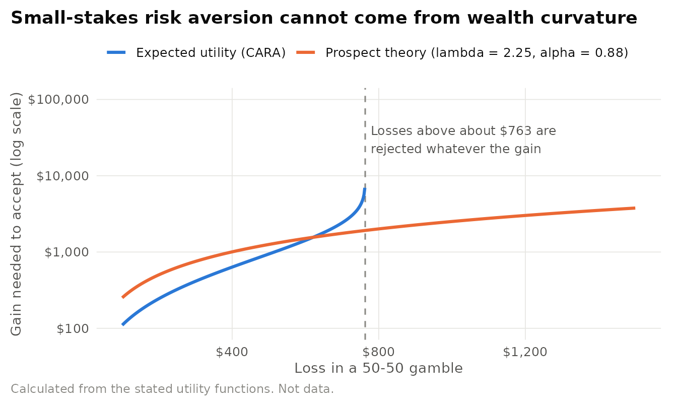
Figure 24.2: Calculated illustration of Rabin’s calibration argument. An expected-utility maximizer with constant absolute risk aversion who rejects a 50-50 lose 100 or gain 110 gamble at every wealth level will reject any 50-50 gamble whose loss exceeds a fixed threshold, however large the gain. A prospect-theory decision maker with the Tversky and Kahneman (1992) value function requires a gain that grows only in proportion to the loss.

Figure 24.2 makes the logic concrete for one special case. Constant absolute risk aversion is the utility function for which rejecting the $100/$110 gamble at every wealth level is exactly consistent. A decision maker with that utility rejects any 50-50 gamble that risks more than about $763, however large the possible gain. Rabin’s theorem shows that a similar, slightly weaker conclusion holds for any concave utility function. A loss-averse decision maker whose value function is defined over gains and losses has no such problem: the gain she requires grows in proportion to the loss.

Is expected utility refuted, or misapplied? Defenders of expected utility make three replies. First, the theory is normative: it describes how a consistent decision maker should choose, and many people who violate the Allais pattern revise their choices when the independence logic is explained. Second, some anomalies can be absorbed by richer expected-utility models, for example by allowing utility over consumption streams, background risk, or narrow bracketing of decisions. Third, a family of non-expected utility theories relaxes independence while keeping much of the structure, including regret theory (Loomes and Sugden 1982), disappointment aversion (Gul 1991), and rank-dependent utility (Quiggin 1982), reviewed by Starmer (2000). Rabin’s calibration result sharpened the debate because it does not depend on laboratory paradoxes: it shows that any expected-utility account of everyday small-stakes risk aversion has implausible implications. The weight of opinion in behavioural economics is that expected utility remains the right normative benchmark but that descriptive models need a reference point.

Treating expected utility as a straw man. Expected utility is not “the assumption that people are rational calculators”. It is a precise, testable model with clear axioms, and its violations are informative precisely because they are specific. When writing about prospect theory, state which axiom or which implication of expected utility a finding contradicts (independence, final-wealth evaluation, or linear probability weighting). Findings that contradict none of them, for example risk aversion over large stakes, are not evidence against expected utility.

24.2 Prospect Theory: The 1979 Model

Core claim. People evaluate risky prospects in two phases. In an editing phase they code outcomes as gains or losses relative to a reference point and simplify the prospects. In an evaluation phase they combine a value function that is concave for gains, convex for losses, and steeper for losses with decision weights that overweight small probabilities and underweight moderate and large ones.

Origins. Psychology and economics. Kahneman and Tversky (1979), building on a decade of collaboration on judgment under uncertainty (Tversky and Kahneman 1974). Framing extensions in Tversky and Kahneman (1981), Kahneman and Tversky (1984), and Tversky and Kahneman (1986).

Level of analysis. Individual choice. Aggregate implications for asset prices, insurance, labour supply, pricing, and policy.

Key constructs. Reference point, gains and losses, value function, diminishing sensitivity, loss aversion, decision weights, certainty effect, reflection effect, isolation effect, editing operations.

Boundary conditions. Formulated for choices among described prospects with few outcomes and known probabilities. The reference point must be identifiable. The editing phase is informal, so predictions depend on how a problem is presented.

Related theories. Expected utility theory, Cumulative prospect theory, Framing theory (Section 26.6), Heuristics and biases (Section 23.2), Mental accounting (Section 23.5).

24.2.1 Origins and intellectual history

By the mid-1970s Kahneman and Tversky had spent several years documenting the heuristics that people use to judge probabilities (Tversky and Kahneman 1974). Prospect theory turned from judgment to choice. Its method was disarmingly simple. The authors posed hypothetical choices between pairs of gambles to student and faculty respondents and reported the share choosing each option. The problems were designed so that expected utility made sharp predictions, typically that the preference in one problem must match the preference in a closely related problem. The data repeatedly showed that it did not. The paper, published in Econometrica in 1979, combined these demonstrations with a formal model that could explain them, which is a large part of why it changed economics as well as psychology (N. C. Barberis 2013).

24.2.2 The empirical demonstrations

Table 24.4 reproduces several of the original choice problems. Payoffs were in Israeli pounds, and the percentages are the shares of respondents choosing each option as reported by Kahneman and Tversky (1979). Read each pair of rows together.

Table 24.4: Selected choice problems from Kahneman and Tversky (1979). Amounts are in Israeli pounds. Percentages are the shares of respondents choosing each option, as reported in the original article.

Problem	Option A	Option B	Choices (A / B)	Pattern illustrated
1	2,500 with p = .33, 2,400 with p = .66, 0 with p = .01	2,400 for sure	18% / 82%	Certainty effect (common consequence)
2	2,500 with p = .33, 0 with p = .67	2,400 with p = .34, 0 with p = .66	83% / 17%	Certainty effect (common consequence)
3	4,000 with p = .80	3,000 for sure	20% / 80%	Certainty effect (common ratio)
4	4,000 with p = .20	3,000 with p = .25	65% / 35%	Certainty effect (common ratio)
7	6,000 with p = .45	3,000 with p = .90	14% / 86%	Preference for the more probable gain
8	6,000 with p = .001	3,000 with p = .002	73% / 27%	Possibility effect: small probabilities
3’	Lose 4,000 with p = .80	Lose 3,000 for sure	92% / 8%	Reflection effect: risk seeking for losses
11	Given 1,000, then win 1,000 with p = .50	Given 1,000, then win 500 for sure	16% / 84%	Isolation effect: same final states as 12
12	Given 2,000, then lose 1,000 with p = .50	Given 2,000, then lose 500 for sure	69% / 31%	Isolation effect: same final states as 11

Four patterns stand out.

1. The certainty effect. Problems 1 and 2 reproduce the Allais pattern with modest stakes. Problems 3 and 4 show a related violation: scaling both winning probabilities by the same factor (from .80 and 1.00 to .20 and .25) reverses the majority preference. Under expected utility, preferences should be unaffected by such a common ratio. Outcomes that are certain receive extra weight relative to outcomes that are merely probable.
2. The possibility effect. Problems 7 and 8 have the same ratio of probabilities and prizes. When winning is probable, most people prefer the more likely, smaller prize. When winning is merely possible, most prefer the larger prize. Very small probabilities are treated differently from moderate ones.
3. The reflection effect. When the signs of the outcomes in Problem 3 are reversed (Problem 3’), the preference reverses as well. A large majority prefer a sure gain of 3,000 to an 80% chance of 4,000, but prefer an 80% chance of losing 4,000 to a sure loss of 3,000. Risk aversion in the domain of gains is accompanied by risk seeking in the domain of losses.
4. The isolation effect. Problems 11 and 12 offer identical distributions of final wealth: in both, the choice is between 1,500 for sure and an even chance of 1,000 or 2,000. Yet respondents chose the sure thing when the problem was framed as gains and the gamble when it was framed as losses. People evaluate changes, not final states, and they evaluate the components of a problem in isolation rather than integrating them with what they already have.

The last result is the most radical. It is a direct contradiction of the assumption, shared by Bernoulli and by von Neumann and Morgenstern, that the carriers of utility are final states of wealth. It also made framing a central topic: if the same decision can be described as a choice between gains or between losses, and the description changes the choice, then description invariance fails (Tversky and Kahneman 1981, 1986).

24.2.3 Core logic: editing and evaluation

The model has two phases (Figure 24.3). In the editing phase, the decision maker organizes and reformulates the options using the operations listed in Table 24.5. In the evaluation phase, each edited prospect is assigned a value and the prospect with the highest value is chosen. For a simple prospect that pays \(x\) with probability \(p\) and \(y\) with probability \(q\), with at most two non-zero outcomes,

\[ V = \pi(p)\,v(x) + \pi(q)\,v(y), \]

where \(v(\cdot)\) is the value function and \(\pi(\cdot)\) is the decision weight attached to each probability. The original paper treated strictly positive and strictly negative prospects separately, segregating the riskless component of the prospect before applying decision weights.

Figure 24.3: The two phases of the 1979 model. Editing codes outcomes relative to a reference point and simplifies the prospects. Evaluation applies the value function to outcomes and the weighting function to probabilities. How a problem is presented (the frame) enters through editing.

Table 24.5: Editing operations in the original prospect theory (Kahneman & Tversky, 1979).

Operation	What it does	Example
Coding	Outcomes are coded as gains or losses relative to a reference point	A salary of 90,000 is a loss for someone who expected 100,000
Combination	Probabilities attached to identical outcomes are added	Two chances of 200, each with p = .25, become one chance of 200 with p = .50
Segregation	A riskless component is separated from the risky component	300 with p = .80 or else 200 becomes a sure 200 plus a .80 chance of 100 more
Cancellation	Components shared by the options are discarded	The common first stage of a two-stage gamble is ignored
Simplification	Probabilities or outcomes are rounded, and extremely unlikely outcomes are dropped	A .49 chance of 101 is treated as an even chance of 100
Detection of dominance	Dominated alternatives are identified and rejected without evaluation	A gamble that is worse in every state is eliminated

24.2.4 The value function

The value function captures three psychological principles.

• Reference dependence. The carriers of value are gains and losses relative to a reference point, not final states of wealth. The reference point is usually the status quo but can be an expectation, an aspiration, or a social norm.
• Diminishing sensitivity. The difference between gains of 100 and 200 feels larger than the difference between gains of 1,100 and 1,200, and the same holds for losses. The function is therefore concave for gains and convex for losses, which produces risk aversion for gains and risk seeking for losses when probabilities are moderate.
• Loss aversion. The function is steeper for losses than for gains. Most people reject a 50-50 gamble to win or lose the same amount, and the gain needed to make such a gamble acceptable is typically about twice the loss.

A convenient parametric form, later estimated by Tversky and Kahneman (1992), is the power function

\[ v(x) = \begin{cases} x^{\alpha} & \text{if } x \ge 0 \\ -\lambda(-x)^{\beta} & \text{if } x < 0, \end{cases} \]

with \(0 < \alpha, \beta \le 1\) governing curvature and \(\lambda \ge 1\) the coefficient of loss aversion. Figure 24.4 shows how the shape responds to each parameter. Lowering \(\alpha\) and \(\beta\) strengthens diminishing sensitivity, so the function flattens away from the reference point. Raising \(\lambda\) rotates the loss limb downward and strengthens the kink at zero. The kink matters as much as the curvature: it generates first-order risk aversion, aversion to small fair gambles that does not vanish as stakes shrink, which expected utility with a smooth utility function cannot produce.

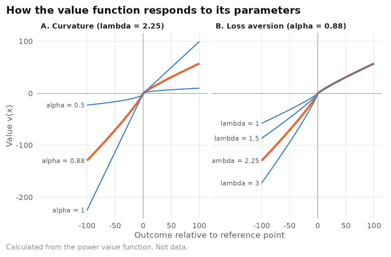
Figure 24.4: Parameter sensitivity of the prospect theory value function. Left: curvature (alpha = beta) varied with lambda fixed at 2.25. Right: loss aversion (lambda) varied with curvature fixed at 0.88. The highlighted curves use the Tversky and Kahneman (1992) estimates.

24.2.5 Decision weights

In the 1979 model, decision weights \(\pi(p)\) are not probabilities. They measure the impact of an event on the desirability of a prospect. The paper derived several properties from the choice data: \(\pi\) is increasing, with \(\pi(0) = 0\) and \(\pi(1) = 1\). Very small probabilities are overweighted, \(\pi(p) > p\), which explains the possibility effect and the joint appeal of lotteries and insurance. Weights display subcertainty, \(\pi(p) + \pi(1 - p) < 1\), which explains the certainty effect. Weights are subproportional: for a fixed ratio of probabilities, the ratio of the corresponding weights is closer to one when probabilities are low than when they are high, which explains the common ratio pattern in Problems 3 and 4 and in Problems 7 and 8. Finally, the function is poorly behaved near the endpoints, where small probabilities may be either ignored in editing or greatly overweighted.

24.2.6 Propositions

The 1979 model can be summarized in six propositions.

• P1 (Reference dependence). Choices depend on outcomes coded as gains and losses relative to a reference point, not on final wealth.
• P2 (Loss aversion). Losses have a greater impact on choice than gains of equal size.
• P3 (Diminishing sensitivity). The marginal impact of a gain or loss declines with its distance from the reference point, producing the reflection effect.
• P4 (Probability weighting). Small probabilities are overweighted and moderate to large probabilities underweighted, with a discontinuity at certainty.
• P5 (Isolation and framing). Components that are shared across options are cancelled, and descriptions that shift the reference point change choices even when final outcomes are identical.
• P6 (Path dependence). Prior gains and losses that have not been fully integrated into the reference point change subsequent risk taking.

P6 is not a formal part of the 1979 model, but it follows from the logic of reference dependence and has strong empirical support. R. H. Thaler and Johnson (1990) documented a house money effect, greater risk taking after a prior gain, and a break-even effect, greater willingness to accept gambles that offer a chance to recover a prior loss. In the high-stakes television game show Deal or No Deal, contestants became less risk averse both after unfavourable outcomes had shattered their expectations and after favourable outcomes had exceeded them, a pattern that is hard to reconcile with expected utility of final wealth (Post et al. 2008).

Timid choices in organizations. Kahneman and Lovallo (1993) argued that managers evaluate risky projects one at a time, in isolation, and therefore apply loss aversion to each project separately. A firm that would happily accept a portfolio of twenty independent projects, each with a positive expected value and a modest chance of loss, may reject every one of them when they are presented sequentially to different managers. The prescription follows from the isolation effect: aggregate decisions into portfolios, evaluate managers on the portfolio rather than on single outcomes, and make the reference point explicit (for example, the hurdle rate rather than zero). Illustrative scenario: a pharmaceutical R&D committee that reviews compounds one at a time, with a separate “kill or continue” vote each quarter, will terminate more promising but risky compounds than a committee that reviews the pipeline as a whole against an explicit expected-value threshold.

Answer Problems 3 and 3’ in Table 24.4 before reading the original percentages. Then ask three friends. Do your answers show the reflection effect? Now rewrite Problem 12 so that it is framed as a gain from a lower starting endowment, and check whether your own preference changes.

24.3 Cumulative Prospect Theory

Core claim. Decision weights apply to cumulative probabilities of outcomes ranked by their attractiveness, separately for gains and losses. This rank-dependent formulation preserves the insights of prospect theory while satisfying first-order stochastic dominance and extending the model to prospects with many outcomes and to uncertainty.

Origins. Decision theory and economics. Tversky and Kahneman (1992), building on rank-dependent utility (Quiggin 1982). Axiomatic weighting functions in Prelec (1998), curvature and elevation in Gonzalez and Wu (1999), and a comprehensive treatment in Wakker (2010).

Level of analysis. Individual choice under risk and uncertainty.

Key constructs. Rank-dependent decision weights, cumulative weighting function, inverse-S shape, curvature (likelihood insensitivity), elevation (optimism), fourfold pattern of risk attitudes, sign dependence.

Boundary conditions. Best supported for described lotteries with known probabilities. When people learn probabilities from experience, rare events are often underweighted (Hertwig et al. 2004). Parameter estimates vary across people, tasks, and elicitation methods.

Related theories. Prospect theory (1979), Expected utility theory, Loss aversion.

24.3.1 Why the original model needed revision

The 1979 model had two technical weaknesses. First, applying a nonlinear weighting function to the probabilities of individual outcomes can violate first-order stochastic dominance: a decision maker might prefer a prospect that is worse in every state of the world. Kahneman and Tversky handled this with an editing rule that eliminates dominated options, but the fix was ad hoc. Second, the model was formulated for prospects with at most two non-zero outcomes, which made it hard to apply to stock returns, insurance contracts, or any continuous distribution.

The solution came from rank-dependent utility (Quiggin 1982). Instead of transforming the probability of each outcome, rank the outcomes from best to worst and transform the cumulative probability of doing at least as well as a given outcome. The decision weight of an outcome is then the marginal contribution of that outcome to the transformed cumulative probability. Tversky and Kahneman (1992) combined this idea with sign dependence: gains and losses are ranked and weighted separately, each with its own weighting function.

24.3.2 The model

Consider a prospect with outcomes ordered \(x_{-m} \le \dots \le x_{-1} < 0 \le x_1 \le \dots \le x_n\) and probabilities \(p_{-m}, \dots, p_n\). Cumulative prospect theory evaluates it as

\[ V = \sum_{i=1}^{n} \pi_i^{+}\, v(x_i) + \sum_{j=1}^{m} \pi_{-j}^{-}\, v(x_{-j}), \]

with decision weights for gains defined from the best outcome downward,

\[ \pi_i^{+} = w^{+}\!\left(p_i + \dots + p_n\right) - w^{+}\!\left(p_{i+1} + \dots + p_n\right), \]

and for losses from the worst outcome upward,

\[ \pi_{-j}^{-} = w^{-}\!\left(p_{-j} + \dots + p_{-m}\right) - w^{-}\!\left(p_{-j+1} + \dots + p_{-m}\right). \]

Because the weights are differences of a monotone function of cumulative probabilities, a prospect that shifts probability toward better outcomes can never be valued less, so dominance is preserved automatically. The inverse-S shape of \(w\) means that the extreme outcomes, the best gain and the worst loss, receive the most overweighting, while intermediate outcomes are underweighted.

Tversky and Kahneman (1992) proposed the one-parameter weighting function

\[ w(p) = \frac{p^{\gamma}}{\left(p^{\gamma} + (1-p)^{\gamma}\right)^{1/\gamma}}, \]

and estimated median parameters from certainty equivalents for a set of gain, loss, and mixed prospects: \(\alpha = \beta = 0.88\) for the value function, \(\lambda = 2.25\) for loss aversion, \(\gamma = 0.61\) for the weighting of gains, and \(\delta = 0.69\) for the weighting of losses. These values remain the default in applied work, although later studies find substantial heterogeneity across individuals and methods (Abdellaoui, Bleichrodt, and Paraschiv 2007, Wakker 2010).

Figure 24.5 plots the Tversky-Kahneman function for several values of \(\gamma\) alongside the one-parameter function axiomatized by Prelec (1998), \(w(p) = \exp\{-(-\ln p)^{a}\}\), whose inverse-S shape always crosses the diagonal at \(p = 1/e \approx 0.37\). Smaller parameter values mean greater curvature: the function is flatter in the middle, so the decision maker is less sensitive to changes in intermediate probabilities and more sensitive to the move from impossibility to possibility and from probability to certainty. Gonzalez and Wu (1999) showed that two psychologically distinct properties are at work. Curvature reflects discriminability, how sensitive a person is to changes in probability. Elevation reflects attractiveness, how much a person likes betting on the chance domain overall. A two-parameter linear-in-log-odds form separates them.

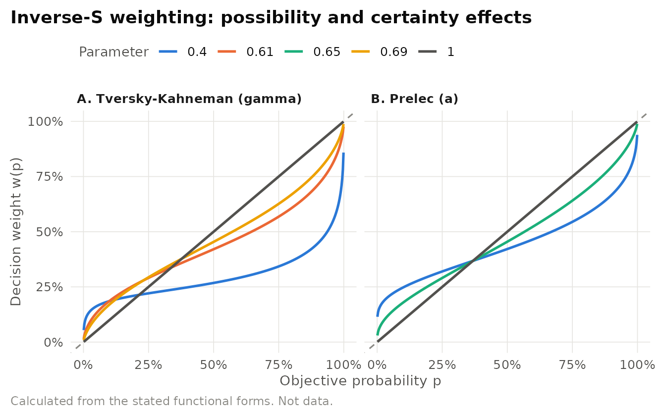
Figure 24.5: Probability weighting functions. Left: the Tversky and Kahneman (1992) form for several values of gamma (0.61 is their median estimate for gains, 0.69 for losses, and 1 is linear weighting). Right: the one-parameter Prelec (1998) form, which crosses the diagonal at 1/e for every parameter value.

Table 24.6 collects the functional forms used most often in empirical work. The choice matters less than is often assumed for qualitative predictions, but it matters a great deal for parameter estimates, which are comparable only within a functional form.

Table 24.6: Common functional forms for the value and probability weighting functions.

Component	Functional form	Parameters	Notes
Value function	Power: x^alpha for gains, -lambda(-x)^beta for losses	alpha, beta (curvature), lambda (loss aversion)	Most common. Loss aversion is only well defined at a unit scale when alpha differs from beta
Value function	Exponential: (1 - exp(-a x)) / a for gains, mirrored for losses	a, b, lambda	Constant absolute sensitivity. Avoids the scaling problem of the power form
Value function	Piecewise linear: x for gains, lambda x for losses	lambda	Isolates loss aversion. Used in many riskless-choice and field studies
Weighting function	Tversky-Kahneman (1992)	gamma (gains), delta (losses)	Inverse-S. Not monotone for very small parameter values
Weighting function	Prelec (1998) one-parameter: exp(-(-ln p)^a)	a	Axiomatically derived. Fixed point at 1/e
Weighting function	Prelec two-parameter: exp(-b(-ln p)^a)	a (curvature), b (elevation)	Separates curvature from elevation
Weighting function	Linear in log odds: d p^g / (d p^g + (1 - p)^g)	g (curvature), d (elevation)	Gonzalez and Wu (1999). Popular in individual-level estimation

24.3.3 How rank-dependent weights work

Figure 24.6 illustrates the decision weights for a four-outcome prospect: win 100 with probability .05, win 40 with probability .30, win 10 with probability .40, and lose 30 with probability .25. The best outcome and the only loss are overweighted relative to their probabilities. The intermediate gains are underweighted. The weights on gains and losses need not sum to one, which is one way prospect theory departs from any model that treats decision weights as beliefs.

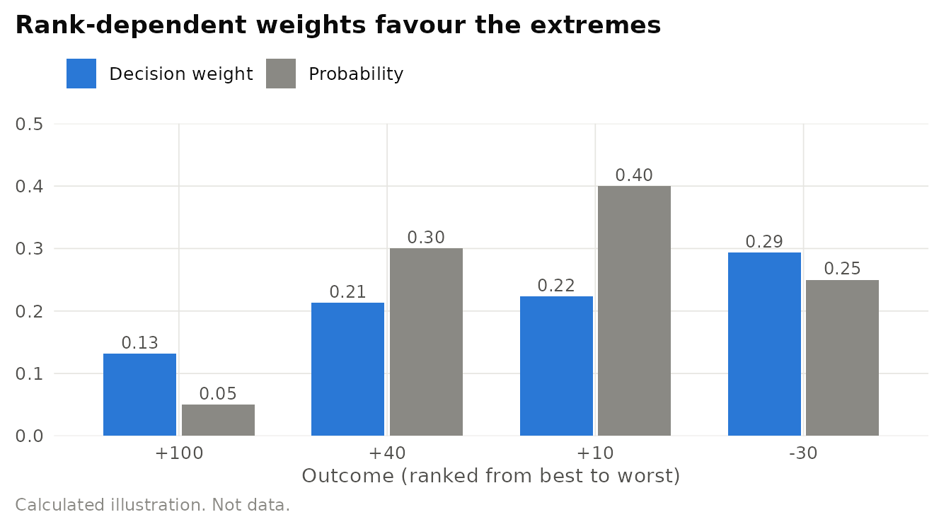
Figure 24.6: Cumulative prospect theory decision weights for an illustrative four-outcome prospect, computed with the Tversky and Kahneman (1992) weighting functions (gamma = 0.61 for gains, delta = 0.69 for losses). Extreme outcomes are overweighted and intermediate outcomes underweighted.

24.3.4 A reusable implementation

The following code implements the cumulative prospect theory value and certainty equivalent of any discrete prospect. It is shown so that readers can reuse it for teaching, for simulation, or as a starting point for estimation. The default parameters are the median estimates of Tversky and Kahneman (1992).

# Value function: power form with loss aversion
pt_value <- function(x, alpha = 0.88, beta = 0.88, lambda = 2.25) {
  ifelse(x >= 0, abs(x)^alpha, -lambda * abs(x)^beta)
}

# Tversky-Kahneman (1992) probability weighting function
pt_weight <- function(p, g) p^g / (p^g + (1 - p)^g)^(1 / g)

# Cumulative prospect theory value of a discrete prospect (outcomes x, probabilities p)
cpt <- function(x, p, alpha = 0.88, beta = 0.88, lambda = 2.25,
                gamma = 0.61, delta = 0.69) {
  stopifnot(length(x) == length(p), abs(sum(p) - 1) < 1e-8)
  w <- numeric(length(x))
  gains <- which(x > 0)
  losses <- which(x < 0)
  if (length(gains)) {                          # rank gains from best to worst
    o <- gains[order(x[gains], decreasing = TRUE)]
    cp <- cumsum(p[o])
    w[o] <- pt_weight(cp, gamma) - pt_weight(c(0, head(cp, -1)), gamma)
  }
  if (length(losses)) {                         # rank losses from worst to best
    o <- losses[order(x[losses])]
    cp <- cumsum(p[o])
    w[o] <- pt_weight(cp, delta) - pt_weight(c(0, head(cp, -1)), delta)
  }
  V <- sum(w * pt_value(x, alpha, beta, lambda))
  ce <- if (V >= 0) V^(1 / alpha) else -(-V / lambda)^(1 / beta)
  list(value = V, certainty_equivalent = ce, weights = w)
}

# Example: the four-outcome prospect used in the figure above
ex <- cpt(x = c(100, 40, 10, -30), p = c(0.05, 0.30, 0.40, 0.25))
round(ex$certainty_equivalent, 2)

#> [1] 1.67

The certainty equivalent of the example prospect is 1.7, compared with an expected value of 13.5. The gap reflects loss aversion: the single loss of 30 is multiplied by \(\lambda = 2.25\) and, as the worst outcome, is also overweighted, so it offsets most of the value of the three gains. The same function reproduces the fourfold pattern of risk attitudes, the theory’s signature prediction for simple prospects (Table 24.7).

fourfold <- expand.grid(p = c(0.05, 0.95), x = c(100, -100))
fourfold$ev <- fourfold$p * fourfold$x
fourfold$ce <- mapply(function(p, x) cpt(c(x, 0), c(p, 1 - p))$certainty_equivalent,
                      fourfold$p, fourfold$x)
fourfold$attitude <- ifelse(fourfold$ce > fourfold$ev, "Risk seeking", "Risk averse")
fourfold |>
  transmute(Prospect = sprintf("%s %d with p = %.2f", ifelse(x > 0, "Win", "Lose"), abs(x), p),
            `Expected value` = round(ev, 1),
            `Certainty equivalent` = round(ce, 1),
            Prediction = attitude) |>
  book_table(caption = "The fourfold pattern computed with cumulative prospect theory and the Tversky and Kahneman (1992) median parameters.")

Table 24.7: The fourfold pattern computed with cumulative prospect theory and the Tversky and Kahneman (1992) median parameters.

Prospect	Expected value	Certainty equivalent	Prediction
Win 100 with p = 0.05	5	10.0	Risk seeking
Win 100 with p = 0.95	95	76.9	Risk averse
Lose 100 with p = 0.05	-5	-8.3	Risk averse
Lose 100 with p = 0.95	-95	-83.1	Risk seeking

Figure 24.7 extends the calculation across the full range of probabilities. Each cell shows the risk premium implied by cumulative prospect theory, expressed as a percentage of the expected value and signed so that positive numbers indicate risk seeking. The four quadrants of the pattern are visible at a glance: risk seeking for low-probability gains (lotteries), risk aversion for high-probability gains (settling a strong lawsuit), risk aversion for low-probability losses (insurance), and risk seeking for high-probability losses (gambling to avoid a sure loss). The same person may therefore buy both insurance and lottery tickets, a long-standing puzzle for expected utility with a single concave utility function.

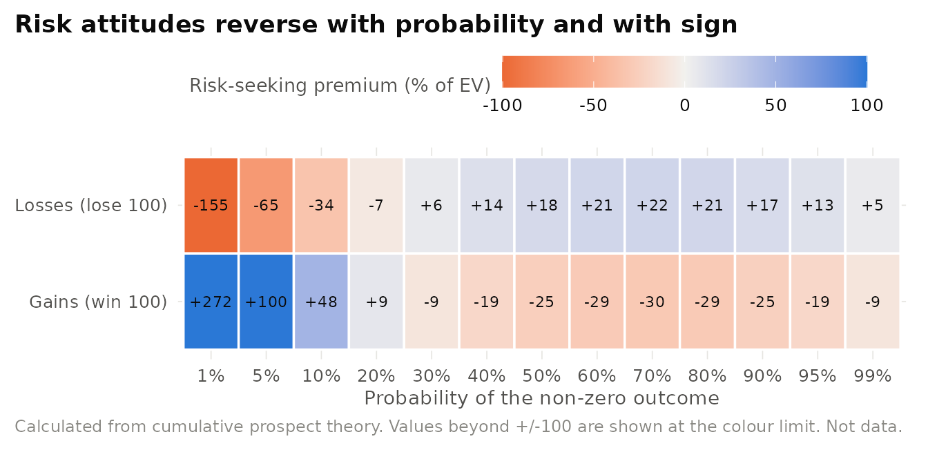
Figure 24.7: The fourfold pattern of risk attitudes. Cells show the risk-seeking premium implied by cumulative prospect theory for a prospect that pays (or costs) 100 with probability p and nothing otherwise, as a percentage of its expected value. Positive values (blue) indicate risk seeking, negative values (orange) risk aversion. Computed from the Tversky and Kahneman (1992) median parameters.

Table 24.8 presents the original and cumulative prospect theory compared.

Table 24.8: Original and cumulative prospect theory compared.

Feature	Prospect theory (1979)	Cumulative prospect theory (1992)
Weights applied to	Probabilities of individual outcomes	Cumulative probabilities of ranked outcomes
Stochastic dominance	Can be violated, handled by an editing rule	Always satisfied
Number of outcomes	At most two non-zero outcomes	Any number, including continuous distributions
Gains and losses	Treated separately for strictly positive or negative prospects	Separate weighting functions, w+ and w-
Uncertainty (unknown probabilities)	Not covered	Covered through capacities (Choquet integrals)
Editing phase	Central and informal	Largely dropped from the formal model
Parameter estimates	None reported	alpha = beta = 0.88, lambda = 2.25, gamma = 0.61, delta = 0.69

Description versus experience. The overweighting of small probabilities is the most robust feature of the weighting function when people choose among described lotteries. Hertwig et al. (2004) asked participants to learn the payoff distributions by sampling from them, as people often do in daily life. In this “decisions from experience” paradigm, rare events were underweighted, in part because small samples often contain no rare event at all. The finding does not falsify cumulative prospect theory, which was formulated for described probabilities, but it limits its domain: predictions about insurance, warnings, or rare disasters depend on whether people know the probabilities or have learned them from their own history. Salience theory offers yet another account, in which the most striking payoffs, rather than the least likely ones, attract excess weight (Bordalo, Gennaioli, and Shleifer 2012).

Estimating prospect theory parameters.

• Elicitation. Certainty equivalents for simple gain and loss prospects identify curvature and weighting. Acceptance of mixed 50-50 gambles identifies loss aversion. Parameter-free methods such as the trade-off method avoid assumptions about functional form (Abdellaoui, Bleichrodt, and Paraschiv 2007, Wakker 2010).
• Estimation. Fit the model by maximum likelihood with a stochastic choice rule (for example, a logit on the difference in prospect values), or by hierarchical Bayesian methods that pool information across participants.
• Identification. Curvature and probability weighting trade off against each other when only a few probabilities are used. Vary probabilities and outcomes independently, and include mixed prospects to pin down \(\lambda\).
• Sample hypothesis. H1. Participants will pay more to reduce a loss probability from .01 to 0 than from .11 to .10 (certainty effect for losses).

24.4 Loss Aversion

Core claim. Losses relative to a reference point have a greater impact on choice and on experience than gains of the same size. In riskless choice, this asymmetry produces the endowment effect (Section 23.4) and status quo bias. In risky choice, it produces aversion to mixed gambles with positive expected value.

Origins. Psychology and economics. Introduced as a property of the value function in Kahneman and Tversky (1979), formalized for riskless choice in Tversky and Kahneman (1991), and documented in exchange experiments by Kahneman, Knetsch, and Thaler (1990) and Kahneman, Knetsch, and Thaler (1991).

Level of analysis. Individual valuation and choice. Dyadic exchange (buyers and sellers, negotiators). Aggregate effects on trading volume, prices, and policy outcomes.

Key constructs. Loss aversion coefficient (\(\lambda\)), willingness to accept versus willingness to pay, reference point, mixed gambles, endowment effect, status quo bias.

Boundary conditions. Weak or absent for money spent as intended and for goods held for exchange (Novemsky and Kahneman 2005), among experienced traders (List 2003), and for very small amounts (Harinck et al. 2007). Its measured size depends on the range of gains and losses in the choice set (Walasek and Stewart 2015).

Related theories. Endowment effect (Section 23.4), Status quo bias, Regulatory focus theory (Section 20.1), Reference-dependent preferences.

24.4.1 Origins and core logic

Loss aversion began as one property of the value function, but it soon became the most widely used idea in behavioural economics. Tversky and Kahneman (1991) showed that it explains choice even when no risk is involved. In their reference-dependent model of riskless choice, preferences over bundles of goods depend on a reference bundle, and each attribute is evaluated with a value function that is steeper for losses. Two implications follow. First, indifference curves are kinked at the reference point, so the rate at which a person will trade one good for another depends on which good she currently holds. Second, the disadvantages of a change loom larger than its advantages, so options that represent a departure from the reference point are penalized.

The best-known demonstration is the mug experiment (Kahneman, Knetsch, and Thaler 1990), discussed in Chapter 23 (Section 23.4): owners of a randomly allocated coffee mug demanded roughly twice as much to sell it as non-owners were willing to pay. Kahneman, Knetsch, and Thaler (1991) connected the endowment effect, status quo bias, and loss aversion as manifestations of a single principle. Rabin’s calibration theorem added a second, independent argument for loss aversion: modest-scale risk aversion in mixed gambles is difficult to explain in any other way (Rabin 2000).

24.4.2 Measuring loss aversion

Loss aversion is easy to describe but surprisingly difficult to measure. The coefficient \(\lambda\) has no single definition. With the power value function, \(\lambda\) is the ratio of the slopes of the loss and gain limbs only at an outcome of one unit, unless \(\alpha = \beta\), so estimates depend on the currency and the functional form. Estimates from mixed gambles also depend on probability weighting: if the decision weights on a 50% chance of gaining and a 50% chance of losing differ, part of what looks like loss aversion may be sign dependent weighting. Riskless measures, such as the ratio of willingness to accept to willingness to pay, capture loss aversion along with transaction costs, strategic misstatement, and reference-price effects. Neuroimaging evidence suggests a neural correlate: in mixed gambles, activity in valuation regions increased with potential gains and decreased more steeply with potential losses, and the asymmetry predicted individual differences in behavioural loss aversion (Tom et al. 2007).

The best current summary of the evidence is a large meta-analysis by A. L. Brown et al. (2024), who collected 607 empirical estimates of the loss aversion coefficient from 150 articles in economics, psychology, neuroscience, and other fields published between 1992 and 2017. Their estimate of the mean coefficient is 1.955, with a 95% probability that the true value lies between 1.820 and 2.102. Few observable features of study design were substantially associated with differences in mean estimates. Loss aversion is therefore real on average and somewhat smaller than the Tversky-Kahneman estimate of 2.25. Figure 24.8 translates these numbers into a behavioural quantity: the gain a decision maker requires to accept a 50-50 gamble with a loss of 100.

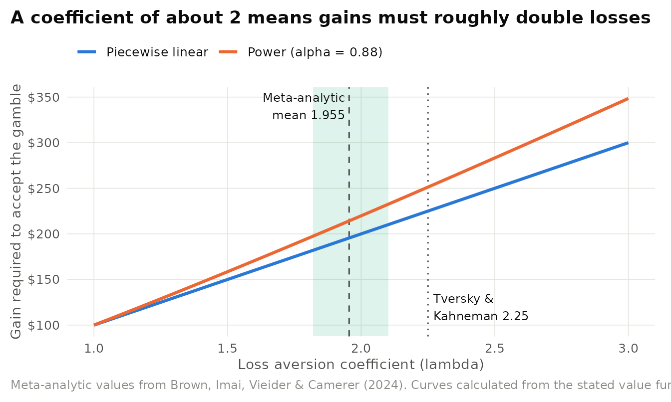
Figure 24.8: What a loss aversion coefficient means in practice: the minimum gain needed to accept a 50-50 gamble that risks a loss of 100, as a function of lambda, under a piecewise-linear value function and under the power value function with alpha = beta = 0.88 (no probability weighting). The shaded band is the 95% interval for the mean coefficient from the meta-analysis of Brown, Imai, Vieider and Camerer (2024), and the dashed line their mean estimate of 1.955. The dotted line marks the Tversky and Kahneman (1992) estimate of 2.25.

24.4.3 Boundaries and moderators

Loss aversion is not a constant of nature. Table 24.9 summarises the principal boundary conditions documented in the literature.

Table 24.9: Boundary conditions and moderators of loss aversion.

Moderator	Finding	Key source
Exchange goods and intended spending	Money spent as intended and goods held for resale are not coded as losses when given up	Novemsky & Kahneman (2005)
Market experience	Experienced traders of sports memorabilia show little or no endowment effect	List (2003)
Stake size	For very small amounts of money, gains can loom larger than losses	Harinck et al. (2007)
Range of outcomes in the task	Loss aversion disappears when gain and loss ranges are symmetric and reverses when losses span a wider range	Walasek & Stewart (2015)
Task format	Small, repeated, or experienced mixed gambles often show little loss aversion	Ert & Erev (2013)
Individual differences	Riskless and risky measures of loss aversion are related at the individual level and vary with personal characteristics	Gächter, Johnson & Herrmann (2022)
Decision maker and decision characteristics	Loss aversion is robust in large samples but systematically moderated	Mrkva et al. (2020)

Ert and Erev (2013) documented how features of the task, such as small stakes and repeated, experienced gambles, reduce measured loss aversion in risky choice. Gächter, Johnson, and Herrmann (2022) measured loss aversion in both riskless and risky tasks for the same individuals and found the two measures to be related and to vary with personal characteristics, which suggests that loss aversion is in part a stable individual difference. Two of the boundaries deserve elaboration. Novemsky and Kahneman (2005) argued that loss aversion applies to goods that are given up as consumption goods, not to goods given up as part of an intended exchange. A shopper who hands over $5 for a sandwich she meant to buy does not experience the $5 as a loss in the same way she would if it were stolen. This boundary explains why ordinary market transactions do not grind to a halt. Walasek and Stewart (2015) tested an account derived from decision by sampling, the idea that the subjective value of an amount depends on its rank among amounts recently encountered (Stewart, Chater, and Brown 2006). In many experiments that estimate loss aversion, the range of possible gains is about twice the range of possible losses, so a given loss ranks higher among losses than the same-sized gain ranks among gains. When Walasek and Stewart equalized the ranges, loss aversion disappeared, and when losses spanned the wider range, the asymmetry reversed. At least part of what is measured as loss aversion in such designs is a property of the choice context rather than of the person.

Figure 24.9: Competing accounts of the asymmetry between losses and gains. The classic account locates it in the value function itself. Alternatives attribute observed asymmetries to attention, to the context of comparison, or to a general preference for inaction. Moderators determine when the asymmetry is observed.

Figure 24.9 organizes the main explanations. The hedonic account is the original: losses simply hurt more than equivalent gains please. An attentional account holds that losses increase on-task attention and arousal, which can affect performance and choice even when they do not receive greater decision weight (Yechiam and Hochman 2013). The sampling account locates the asymmetry in the distribution of outcomes people compare against (Stewart, Chater, and Brown 2006, Walasek and Stewart 2015). The inertia account holds that many apparent demonstrations of loss aversion reflect a reluctance to act (Gal 2006).

The loss of loss aversion? Gal and Rucker (2018b) argued that the evidence does not support loss aversion as a general principle. Building on Gal (2006), they contended that the endowment effect and status quo bias can be explained by psychological inertia, that losses do not have greater impact than gains in many studies once the status quo is not the default, and that the field had accepted the principle with too little scrutiny. The Journal of Consumer Psychology published commentaries alongside the critique. Simonson and Kivetz (2018) agreed that loss aversion is contingent but argued that its contingency does not make it less real or less useful. Higgins and Liberman (2018) argued that the debate turns on how reference points are construed and on the decision maker’s motivational state. Gal and Rucker (2018a) replied by calling for a more contrarian science. In a later response, Mrkva et al. (2020) reported large-sample evidence that loss aversion is robust but systematically moderated by characteristics of the decision maker and the decision, so that the productive question is when and for whom losses loom larger. The meta-analysis of A. L. Brown et al. (2024) supports this view: the average coefficient is reliably above one, but the dispersion across studies is large. The debate has sharpened the theory rather than ended it: researchers are now expected to specify the reference point, rule out inertia, and consider outcome-range artefacts before invoking loss aversion.

24.4.4 Applications in business

Sales and production bonuses framed as losses. Hossain and List (2012) ran a natural field experiment in a Chinese high-tech manufacturing facility. Workers received conditional bonuses framed either as gains (a bonus paid if productivity met a target) or as losses (a provisional bonus that would be taken back if the target was missed). Both framings raised productivity. Teams responded more strongly to the loss frame, and the framing effect alone raised total team productivity by about 1%, with no sign of fading over the study period. In education, Fryer et al. (2022) paid teachers an up-front bonus that had to be returned if their students did not improve sufficiently. Pooling two waves, the loss-framed incentive improved mathematics achievement by an estimated 0.124 standard deviations, with large effects in the first wave and none in the second, while a gain-framed bonus produced a smaller effect of about 0.051 standard deviations that was not statistically significant. For managers designing sales compensation, the lesson is that pre-paid, claw-back incentives can motivate more than equivalent end-of-period bonuses, but they raise fairness, retention, and legal concerns, and their effects may not persist.

Calling every negative frame “loss aversion”. A message that mentions a loss, a price above some benchmark, or a bad outcome is not evidence of loss aversion unless (1) a reference point is specified, (2) gains and losses of comparable magnitude are compared, and (3) alternative explanations such as inertia, attention, or the range of outcomes are ruled out. Many published “loss aversion” effects are better described as negativity effects or framing effects.

24.5 Reference-Dependent Preferences

Core claim. People derive utility from outcomes themselves (consumption utility) and from comparing outcomes with a reference point (gain-loss utility). In the leading modern formulation, the reference point is the person’s recent rational expectations about outcomes, so that surprises, not outcomes alone, generate feelings of gain and loss.

Origins. Economics. Kőszegi and Rabin (2006) and Kőszegi and Rabin (2007), building on Kahneman and Tversky (1979) and Tversky and Kahneman (1991). Reviewed in O’Donoghue and Sprenger (2018).

Level of analysis. Individual choice and effort. Market implications for pricing, labour supply, insurance, and job search.

Key constructs. Reference point (status quo, expectation, goal, norm), consumption utility, gain-loss utility, stochastic reference point, personal equilibrium, choice-acclimating equilibrium, first-order risk aversion.

Boundary conditions. Expectations must be formed before the outcome is realized and must be salient. Evidence for expectations as reference points is mixed in replication, and the reference point may adapt with a lag.

Related theories. Loss aversion, Goal-setting theory (Section 19.4), Social comparison theory (Section 22.1), Expectancy-disconfirmation (Section 27.1).

24.5.1 What is the reference point?

Prospect theory says that outcomes are coded relative to a reference point but says little about where the reference point comes from. Kahneman and Tversky usually took it to be the status quo while acknowledging that aspirations, expectations, and norms could play the role. This flexibility is the theory’s greatest strength and its greatest weakness. Applied work has used at least the candidates listed in Table 24.10.

Table 24.10: Candidate reference points used in research on reference-dependent preferences.

Reference point	Definition	Illustrative evidence
Status quo	Current endowment or default option	Endowment effect, default effects (Kahneman et al., 1990, Madrian & Shea, 2001)
Purchase price	Price originally paid for an asset	Disposition effect, condominium sellers (Odean, 1998, Genesove & Mayer, 2001)
Expectations	Recent beliefs about likely outcomes	Effort provision, football and family violence (Abeler et al., 2011, Card & Dahl, 2011)
Goals	Self-set or assigned targets	Goals as reference points, marathon bunching (Heath et al., 1999, Allen et al., 2017)
Salient numbers	Par, round numbers, thresholds	Golf putting, four-hour marathons (Pope & Schweitzer, 2011, Allen et al., 2017)
Past prices	Last price paid or average past price	Reference price effects in brand choice (Hardie et al., 1993)
Recent income	Earnings in the recent past	Job search around benefit cuts (DellaVigna et al., 2017)
Fair or past wages	Wage demanded or previously received	Police performance after arbitration losses (Mas, 2006)

Heath, Larrick, and Wu (1999) made the link between goals and reference points explicit: a goal inherits the properties of the value function. Because of diminishing sensitivity, a unit of progress is worth more the closer one is to the goal, so people work harder as they approach it, and because of loss aversion, the shortfall from a missed goal is felt as a loss. This idea connects prospect theory to goal-setting theory (Section 19.4) and the goal-gradient hypothesis (Section 19.5).

24.5.2 The Kőszegi-Rabin model

Kőszegi and Rabin (2006) proposed a disciplined answer to the reference-point question. A person’s utility from an outcome \(c\) given a reference outcome \(r\) is

\[ u(c \mid r) = m(c) + \mu\big(m(c) - m(r)\big), \]

where \(m(\cdot)\) is ordinary consumption utility and \(\mu(\cdot)\) is gain-loss utility, typically piecewise linear with slope \(\eta\) for gains and \(\eta\lambda\) for losses. The key move is to set the reference point equal to the person’s recent rational expectations about outcomes. Because expectations can be uncertain, the reference point is itself a probability distribution \(F\), and an outcome is compared with every outcome the person expected, weighted by its probability:

\[ U(c \mid F) = \int u(c \mid r)\, dF(r). \]

Expectations must also be internally consistent. A personal equilibrium is a plan that the person would want to carry out given that she expects to carry it out. This makes the reference point endogenous to the economic environment. The model predicts that willingness to pay for a good rises with the expected probability of buying it and with expected prices, and that a worker is less likely to keep working when income so far is unexpectedly high but more likely to show up when expected income is high (Kőszegi and Rabin 2006). Kőszegi and Rabin (2007) applied the framework to risk. When a risk is a surprise, the model reproduces classical prospect theory. When a risk is anticipated and the person can plan for it, it implies first-order risk aversion, and a prior expectation of taking risk reduces aversion both to that risk and to additional risk.

Figure 24.10 illustrates the core intuition. A person who will earn either 0 or 100 evaluates an outcome of 50 differently depending on how likely she thought the high outcome was. When she expected 0, an outcome of 50 is a pure gain. When she expected 100, the same outcome is a pure loss. With uncertain expectations, it is a mixture of both.

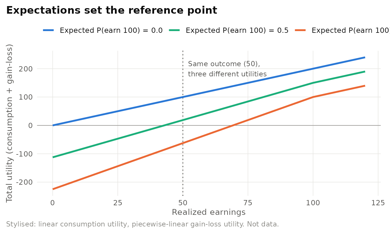
Figure 24.10: Stylised illustration of expectation-based reference points (Kőszegi & Rabin, 2006). A person expects to earn 100 with probability q and 0 otherwise. Total utility of a realized outcome equals consumption utility plus gain-loss utility relative to every outcome she expected, with eta = 1 and lambda = 2.25. The same outcome yields lower utility when higher earnings were expected.

24.5.3 Evidence from the laboratory

2 tested the expectations hypothesis directly. Participants performed a tedious counting task and decided when to stop. When they stopped, a coin flip determined whether they received their accumulated piece-rate earnings or a fixed payment announced in advance. The fixed payment manipulated expectations without changing the piece rate. When the fixed payment was high, participants worked longer and earned more than when it was low, as models of expectation-based reference dependence predict. Ericson and Fuster (2011) found that manipulating the expected probability of keeping a good changed valuations and trading in the predicted direction. Gill and Prowse (2012) estimated a structural model of disappointment aversion in a real-effort competition and found that effort responded to a rival’s effort in the way expectation-based reference points imply. Sprenger (2015) showed that risk attitudes depend on whether the reference point is a certain amount or a lottery, an “endowment effect for risk” consistent with stochastic reference points.

The laboratory evidence is not uniform. Heffetz and List (2014) found that manipulating the probability of keeping an object did not change the endowment effect in their experiments, which pointed to ownership rather than expectations as the operative reference point. Gneezy et al. (2017) extended the Abeler et al. design to a wider range of fixed payments and found that the predicted relationship between expectations and effort did not generalize. The present consensus is that expectations can serve as reference points, but which reference point operates, and how quickly it adapts, depends on the setting (O’Donoghue and Sprenger 2018).

24.5.4 Evidence from the field

Field studies have been central to the case for reference dependence because they involve real stakes, experienced decision makers, and outcomes that matter to them. Table 24.11 summarises influential studies.

Table 24.11: Selected field evidence on reference-dependent preferences.

Study	Setting	Reference point	Finding
Pope & Schweitzer (2011)	PGA Tour, over 2.5 million putts	Par on each hole	Golfers are more accurate putting for par than for birdie from the same distance
Allen et al. (2017)	About 9.8 million marathon finishing times	Round-number times (e.g., four hours)	Finishing times bunch just before round numbers, driven by effort near the finish
Card & Dahl (2011)	Police reports on National Football League Sundays	Pregame point spread (expected result)	Upset losses raise at-home male violence against partners by about 10%. Upset wins have little effect
Genesove & Mayer (2001)	Boston condominiums, 1990s	Original purchase price	Owners facing nominal losses set higher asking prices and sell more slowly
Mas (2006)	New Jersey police after final-offer arbitration	Wage demanded	Performance declined after unions lost arbitration
Fehr & Goette (2007)	Zurich bicycle messengers, temporary wage increase	Daily income target	Messengers worked more shifts but less effort per shift, a decline found among loss-averse messengers
DellaVigna et al. (2017)	Hungarian unemployment insurance reform	Recent income	Job search responds to benefit cuts as if the reference point adapts to recent income

Labour markets supply several of the entries. Mas (2006) found that the performance of New Jersey police declined after their unions lost final-offer arbitration, as if the wage they had demanded served as a reference point. Fehr and Goette (2007) offered Zurich bicycle messengers a temporary wage increase: the messengers worked more shifts but delivered less per shift, and the decline in effort per shift was concentrated among messengers who were loss averse in separate lottery choices, consistent with a daily income target. DellaVigna et al. (2017) studied a reform of Hungarian unemployment insurance and found that job search responded to benefit cuts as if the reference point were recent income that adapts over time.

The football study is a particularly clean test of expectation-based reference points. Card and Dahl (2011) used betting markets to measure what fans expected before each game. Losses that were expected to be close had small and insignificant effects on domestic violence, and upset wins had little effect, but upset losses, defeats when the home team was predicted to win by four or more points, were followed by a 10% increase in at-home violence by men against their wives and girlfriends. The asymmetry between upset wins and upset losses mirrors loss aversion, and the dependence on the point spread mirrors expectation-based reference points.

Do taxi drivers target a daily income? C. Camerer et al. (1997) studied New York City cab drivers, whose hourly earnings vary from day to day but are correlated within a day. A standard life-cycle model predicts that drivers work longer on high-wage days. Instead, estimated wage elasticities were significantly negative in two of three samples, averaging about minus one among inexperienced drivers. The authors interpreted this as evidence that drivers take decisions “one day at a time” and quit when they reach a loose daily income target, a reference point below which shortfalls feel like losses. Farber (2008) estimated a reference-dependent model directly and found that, although a daily reference income may exist, it varies so much from day to day and most shifts end so far from it that reference dependence has little predictive power. Using the complete record of New York taxi trips from 2009 to 2013, Farber (2015) found that drivers generally respond positively to both anticipated and unanticipated increases in earnings opportunities, that stopping depends much more on hours worked than on income earned, and that drivers who remain in the industry quickly learn to behave like optimizers. Two lines of work keep the reference-dependence account alive. V. P. Crawford and Meng (2011) showed that a model with expectation-based targets for both hours and income, in the spirit of Kőszegi and Rabin, reconciles much of the evidence. Thakral and Tô (2021) found that the likelihood of ending a shift responds more to earnings accumulated recently than to earlier earnings, consistent with a reference point that adapts during the day. The debate illustrates a general lesson: reference dependence is easy to assert and hard to identify, and its empirical success depends on modelling how the reference point is formed.

Pricing when customers expect prices. If the reference point is what customers expect to pay, firms face a demand curve with a kink at the expected price: a price slightly above expectations is coded as a loss and reduces demand sharply, while a price slightly below is only a modest gain. Heidhues and Kőszegi (2008) showed that, with loss-averse consumers and expectation-based reference points, competing firms may charge the same “focal” price even when their costs differ, and keep prices sticky as costs change. This logic explains why many retailers prefer stable everyday prices to frequent small changes, why price increases are often bundled with visible product changes, and why promotions that are too frequent can lower the reference price (Section 27.11) itself (Kalyanaram and Winer 1995). Illustrative scenario: a subscription software firm that raises its monthly price from $10 to $11 will see more churn among customers who expected $10 than a firm that launched at $11, even though the final price is identical.

Studying reference points.

• Sample hypotheses. H1. Sales representatives will exert more effort in the final week of a quarter when they are just below their quota than when they are just above it. H2. Customers whose renewal price exceeds the price they paid last year will churn more than customers facing the same price without a prior lower price. H3. Upset losses in customer satisfaction surveys (scores below expectations set by marketing claims) will reduce repurchase more than upset gains increase it.
• Designs. Bunching estimators at salient thresholds (round numbers, quotas, tax kinks). Regression discontinuity around reference points. Experiments that manipulate expectations independently of outcomes, as in
  2. Structural models that let the reference point adapt.
• Measures. Expected outcomes (forecasts, betting lines, guidance), distance from goals, past prices and wages, and self-reported reference points.

Choosing the reference point after seeing the data. Because almost any number can be a reference point, a study that searches for one that “works” will usually find it. Pre-register the reference point, justify it from institutional features or measured expectations, and show that alternative candidates do not fit equally well.

24.6 Status Quo Bias

Core claim. People disproportionately choose the option that represents the current state of affairs or the default, even when switching is cheap and the alternatives are at least as good.

Origins. Economics and decision science. Named and documented by W. Samuelson and Zeckhauser (1988). Linked to loss aversion by Kahneman, Knetsch, and Thaler (1991) and Tversky and Kahneman (1991).

Level of analysis. Individual choice, with large aggregate effects in organizations and public policy (retirement saving, insurance, organ donation, subscriptions).

Key constructs. Status quo, default option, loss aversion, inertia, transaction and switching costs, regret, implied endorsement.

Boundary conditions. Weaker when the status quo is clearly inferior, when active choice is required, when decision makers are expert or highly motivated, and when switching is made salient and easy.

Related theories. Endowment effect (Section 23.4), Choice architecture (Section 23.10), Loss aversion, Escalation of commitment (Section 14.2).

24.6.1 Core logic and evidence

W. Samuelson and Zeckhauser (1988) presented participants with hypothetical decision problems, such as how to invest an inheritance, in two versions. In the neutral version, all options were presented on an equal footing. In the status quo version, one option was described as the current state of affairs. Options were chosen substantially more often when they were designated as the status quo. The authors then showed the same pattern in field data: in employee health plans and in retirement allocations, people rarely revisited choices they had made years earlier, even as their circumstances and the options changed.

Loss aversion offers a natural explanation (Kahneman, Knetsch, and Thaler 1991). If the status quo is the reference point, then every alternative involves giving up some features of the current option (losses) in exchange for others (gains). Because the losses loom larger, the current option wins unless the alternative is clearly better. But status quo bias is overdetermined. Table 24.12 lists the main explanations and the evidence that would distinguish among them, and Figure 24.11 shows how they combine.

Table 24.12: Explanations for status quo bias.

Explanation	Mechanism	Distinguishing prediction
Loss aversion	Departures from the reference point are coded as losses on some attributes	Bias larger when alternatives trade off attributes (some better, some worse)
Inertia and procrastination	Acting requires effort and attention that people postpone	Bias shrinks when active choice is required or switching is made effortless
Transaction and search costs	Switching has real costs	Bias scales with the cost of switching
Implied endorsement	Defaults are read as advice from the choice architect	Bias larger when the default setter is trusted and the decision maker is uncertain
Anticipated regret	Bad outcomes after switching feel worse than after staying	Bias larger when outcomes will be observed and attributed to the choice
Psychological inertia	A general preference for not acting without a compelling reason	Bias appears even when no losses are involved (Gal, 2006)

Figure 24.11: Multiple pathways to status quo bias. Loss aversion is one route among several, and choice architects can intervene at each one (active choice, simplified switching, careful selection of defaults).

Insurance framing. E. J. Johnson et al. (1993) documented a natural experiment in automobile insurance. Around 1990, New Jersey and Pennsylvania both offered drivers a choice between a cheaper policy that limited the right to sue for pain and suffering and a more expensive policy that preserved the full right to sue. In New Jersey, the default was the limited policy. In Pennsylvania, the default was the full policy. In each state, most drivers ended up with their state’s default, so that two economically similar populations held very different coverage. The same paper reported laboratory evidence that insurance choices violate basic laws of probability. In one study, people were willing to pay more for flight insurance covering death from terrorism than for insurance covering death from any cause, which necessarily includes terrorism.

Retirement saving. Madrian and Shea (2001) studied a large US firm that changed its 401(k) plan from opt-in to automatic enrollment for new employees. Participation rose sharply, from about 37% to 86% among employees with comparable tenure. Many automatically enrolled employees also kept both the default contribution rate (3% of pay) and the default investment (a money market fund), even though few employees hired before the change had chosen that combination. The authors attributed the effect to inertia and to employees’ perception of the default as investment advice. The study helped launch the modern policy interest in defaults, discussed in Choice architecture (Section 23.10), and inspired Save More Tomorrow, which asks employees to commit in advance to raising their saving rate out of future pay increases, so that saving more never requires a cut in take-home pay that would be coded as a loss (R. H. Thaler and Benartzi 2004).

401(k) auto-enrollment. Automatic enrollment converts status quo bias from an obstacle into a lever. The design lessons from Madrian and Shea (2001) and R. H. Thaler and Benartzi (2004) are now standard practice. (1) Make participation the default. (2) Choose the default contribution rate and fund carefully, because many employees will keep them, so a low default rate can reduce saving for employees who would otherwise have chosen more. (3) Use automatic escalation tied to pay increases, so that higher contributions are never experienced as a loss of take-home pay. (4) Preserve easy opt-out, which keeps the policy libertarian and protects employees for whom the default is wrong. The same logic underlies auto-renewal of subscriptions, but there the firm, not the customer, benefits from inertia, which is why regulators increasingly require easy cancellation.

Free trials and the reference point. A free trial combines three prospect-theory mechanisms. During the trial the customer acquires a sense of ownership, so cancelling is coded as giving up something already possessed (Endowment effect (Section 23.4)). If the trial converts automatically into a paid subscription, continuing becomes the status quo. And the first payment, which arrives after the customer has adapted to having the service, may be evaluated against a reference point of zero cost. Illustrative scenario: a streaming service comparing an opt-in trial (customers must actively subscribe at the end) with an opt-out trial (customers are charged unless they cancel) should expect higher conversion under opt-out, but also more complaints, chargebacks, and regulatory risk, and lower retention among customers who converted only through inertia.

24.7 Myopic Loss Aversion

Core claim. Investors who are loss averse and who evaluate their portfolios frequently will find risky assets unattractive, because frequent evaluation reveals many short-run losses. The combination, myopic loss aversion, can explain why stocks must offer a large premium over bonds to be held.

Origins. Finance and behavioural economics. Benartzi and Thaler (1995), motivated by the equity premium puzzle of Mehra and Prescott (1985). Experimental tests in Gneezy and Potters (1997) and R. H. Thaler et al. (1997).

Level of analysis. Individual investors, with implications for asset prices and for the design of pension plans and investment platforms.

Key constructs. Loss aversion, evaluation period, narrow framing (choice bracketing), equity premium, feedback frequency.

Boundary conditions. Requires that gains and losses be evaluated over short horizons and in isolation from other wealth. Weaker when investors can commit to long horizons or receive aggregated feedback.

Related theories. Loss aversion, Mental accounting (Section 23.5), Behavioral finance (Section 16.8), Portfolio theory (Section 16.1).

24.7.1 The equity premium puzzle

Over long periods, US stocks have earned far higher average returns than short-term government bonds. Mehra and Prescott (1985) showed that standard consumption-based asset pricing models with plausible levels of risk aversion can account for only a small fraction of the historical premium: matching it requires a degree of risk aversion that seems implausibly high. This is the equity premium puzzle.

Benartzi and Thaler (1995) offered a behavioural explanation built from two ingredients. First, investors are loss averse. Second, even investors with long horizons evaluate their portfolios frequently. Stocks are volatile, so the more often their value is checked, the more often it shows a loss, and loss aversion makes each observed loss painful. Using simulations based on historical returns and the prospect theory parameters of Tversky and Kahneman (1992), they found that the size of the equity premium is consistent with those parameters if investors evaluate their portfolios annually. The idea echoes a famous anecdote, discussed by Benartzi and Thaler (1999), in which a colleague of Paul Samuelson declined a single favourable bet but said he would accept a hundred of them.

Figure 24.12 reproduces the logic in a stylised simulation. It asks how large an equity premium is needed for a loss-averse investor to be indifferent between stocks and a riskless bond when gains and losses are evaluated over horizons from one month to ten years. Table 24.13 shows the reason: the probability of observing a loss falls steeply as the evaluation period lengthens.

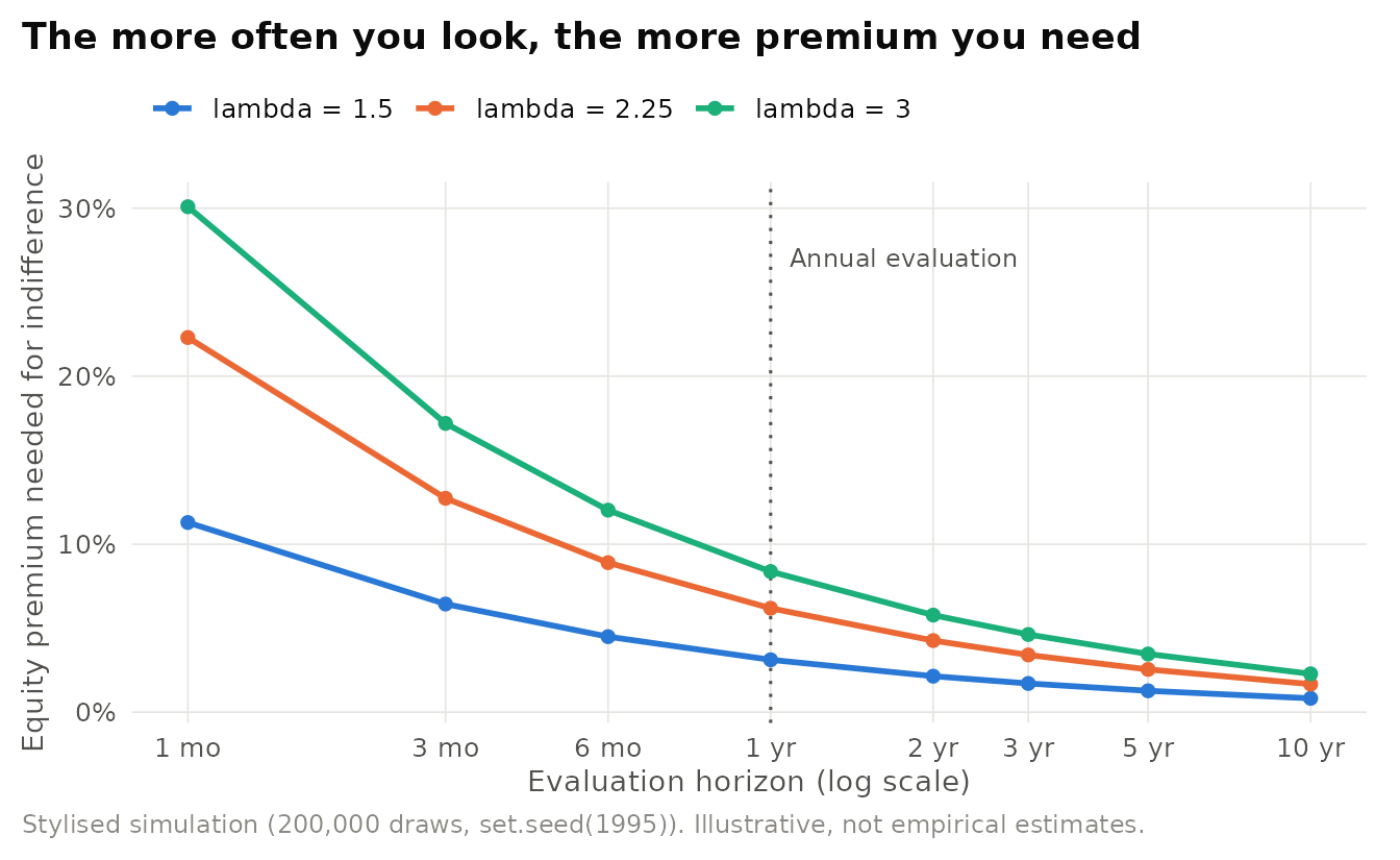
Figure 24.12: Stylised simulation of myopic loss aversion. For each evaluation horizon, the curve shows the annual equity premium at which a loss-averse investor with a piecewise-linear value function is indifferent between stocks and a riskless bond. Shorter horizons reveal more losses and require larger premiums. Stylised assumptions: lognormal stock returns with 20% annual volatility, a 1% riskless rate, no probability weighting. This is not the calibration of Benartzi and Thaler (1995).

Table 24.13: Stylised probability that a stock portfolio shows a nominal loss over different evaluation horizons (lognormal returns, 7% expected annual return, 20% volatility). Illustrative values, not historical estimates.

	Horizon	Probability of a loss
1 day	1 day	49%
1 month	1 month	47%
1 quarter	1 quarter	45%
1 year	1 year	40%
5 years	5 years	29%
10 years	10 years	21%
20 years	20 years	13%

24.7.2 Experimental evidence

The theory makes a sharp, testable prediction: holding the investment opportunity constant, people who receive feedback and make decisions more frequently should take less risk. Table 24.14 summarises the key tests.

Table 24.14: Experimental tests of myopic loss aversion.

Study	Design	Finding
Gneezy & Potters (1997)	Repeated bets on a favourable lottery, with outcomes evaluated each round or in blocks of rounds	The more frequently returns were evaluated, the less participants bet
Thaler, Tversky, Kahneman & Schwartz (1997)	Allocation between a risky and a safe fund, learned from experience, with feedback at different frequencies	Investors with the most frequent feedback took the least risk and earned the least. Eliminating losses increased risk taking
Haigh & List (2005)	Gneezy-Potters design with professional futures and options traders and students	Traders displayed myopic loss aversion to a greater extent than students
Benartzi & Thaler (1999)	Retirement allocation with one-year versus long-run return distributions	Showing the long-run distribution increased allocations to stocks

The professional trader result is especially important because it contradicts the common presumption that market experience eliminates behavioural anomalies. Haigh and List (2005) expected traders to show less myopic loss aversion than students. They found more. Asset pricing models have since incorporated these ideas more formally. N. Barberis, Huang, and Santos (2001) embedded loss aversion over financial wealth fluctuations, with a reference point that depends on prior gains and losses, into an equilibrium model that generates a high equity premium and volatile, predictable returns. N. Barberis, Huang, and Thaler (2006) argued that narrow framing, evaluating a gamble in isolation from other risks, is needed to explain why people reject small independent gambles and why many households do not hold stocks at all.

Investor feedback and platform design. Myopic loss aversion implies that the frequency and format of portfolio feedback is a design variable with consequences for investor welfare. Retirement plan statements that display long-horizon return distributions, apps that default to showing annual rather than daily performance, and communications that aggregate accounts rather than reporting each fund separately all lengthen the effective evaluation period. Illustrative scenario: a robo-advisor testing two dashboards, one showing daily changes in red and green and one showing progress toward a retirement goal updated quarterly, would expect the second to produce fewer panic sales after market declines and higher equity allocations, consistent with Gneezy and Potters (1997) and R. H. Thaler et al. (1997). The ethical question is whether hiding short-run volatility serves investors or simply keeps assets under management.

Use the simulation code behind Figure 24.12 (change sigma, rf, or the lambda values) to find the evaluation horizon at which a loss-averse investor with \(\lambda = 2\) would hold stocks at an annual premium of 4%. How does the answer change if volatility is 15% rather than 20%?

24.8 Disposition Effect

Core claim. Investors are more likely to sell assets that have risen in value since purchase than assets that have fallen, holding losers too long and selling winners too early.

Origins. Finance. Named by Shefrin and Statman (1985), documented in brokerage data by Odean (1998), in housing by Genesove and Mayer (2001), and in the laboratory by M. Weber and Camerer (1998).

Level of analysis. Individual investors and property owners, with implications for trading volume, price momentum, and real estate markets.

Key constructs. Purchase price as reference point, realized versus paper gains and losses, proportion of gains realized (PGR), proportion of losses realized (PLR), realization utility, regret.

Boundary conditions. Weaker among more experienced and sophisticated investors, and reversed in contexts with strong tax incentives to realize losses. Its link to prospect theory’s value function is debated.

Related theories. Loss aversion, Mental accounting (Section 23.5), Escalation of commitment (Section 14.2), Behavioral finance (Section 16.8).

24.8.1 Origins and core logic

Shefrin and Statman (1985) coined the term disposition effect and proposed an explanation combining four elements: prospect theory (with the purchase price as reference point), mental accounting (each stock held in its own account), regret aversion (realizing a loss confirms a mistake), and self-control (investors may need rules to overcome the reluctance to sell losers). The prospect theory logic is that a stock trading above its purchase price is in the concave, risk-averse region of the value function, which encourages locking in the gain, while a stock trading below its purchase price is in the convex, risk-seeking region, which encourages holding on in the hope of breaking even.

24.8.2 Evidence

Odean (1998) developed the standard empirical test using the trading records of 10,000 accounts at a large discount brokerage. On each day an investor sold any stock, every stock in the portfolio was classified as a realized gain, a paper (unrealized) gain, a realized loss, or a paper loss. The proportion of gains realized, PGR, is the number of realized gains divided by realized plus paper gains. The proportion of losses realized, PLR, is defined analogously. Odean found that investors realized gains at a much higher rate than losses, that the pattern was not explained by portfolio rebalancing or by the higher trading costs of low-priced stocks, and that it was not justified by subsequent performance: the winners investors sold went on to outperform the losers they kept. The code below implements the PGR and PLR calculation for any position-level dataset and applies it to simulated data.

# PGR and PLR from position-level data (Odean, 1998).
# d: one row per position held on a day on which the investor sold something,
#    with logical columns `gain` (price above purchase price) and `sold`.
pgr_plr <- function(d) {
  rg <- sum(d$gain & d$sold)
  pg <- sum(d$gain & !d$sold)
  rl <- sum(!d$gain & d$sold)
  pl <- sum(!d$gain & !d$sold)
  pgr <- rg / (rg + pg)
  plr <- rl / (rl + pl)
  se <- sqrt(pgr * (1 - pgr) / (rg + pg) + plr * (1 - plr) / (rl + pl))
  data.frame(PGR = pgr, PLR = plr, Difference = pgr - plr, `t statistic` = (pgr - plr) / se,
             check.names = FALSE)
}

# Simulated (illustrative) investors: selling propensity rises with the size of
# the unrealized return in either direction and jumps just above zero.
set.seed(1998)
sim <- data.frame(investor = rep(1:400, each = 8 * 30),
                  day = rep(rep(1:30, each = 8), 400),
                  ret = rnorm(400 * 8 * 30, 0.02, 0.25))
sim$gain <- sim$ret > 0
sim$sold <- runif(nrow(sim)) < plogis(-2.8 + 0.6 * sim$gain + 2.5 * abs(sim$ret))
sale_days <- unique(sim[sim$sold, c("investor", "day")])
sim_sd <- merge(sim, sale_days)                     # keep only days with a sale
round(pgr_plr(sim_sd), 3)

#>     PGR   PLR Difference t statistic
#> 1 0.234 0.143      0.091       29.86

Figure 24.13 shows the stylised disposition effect in simulated trading data.

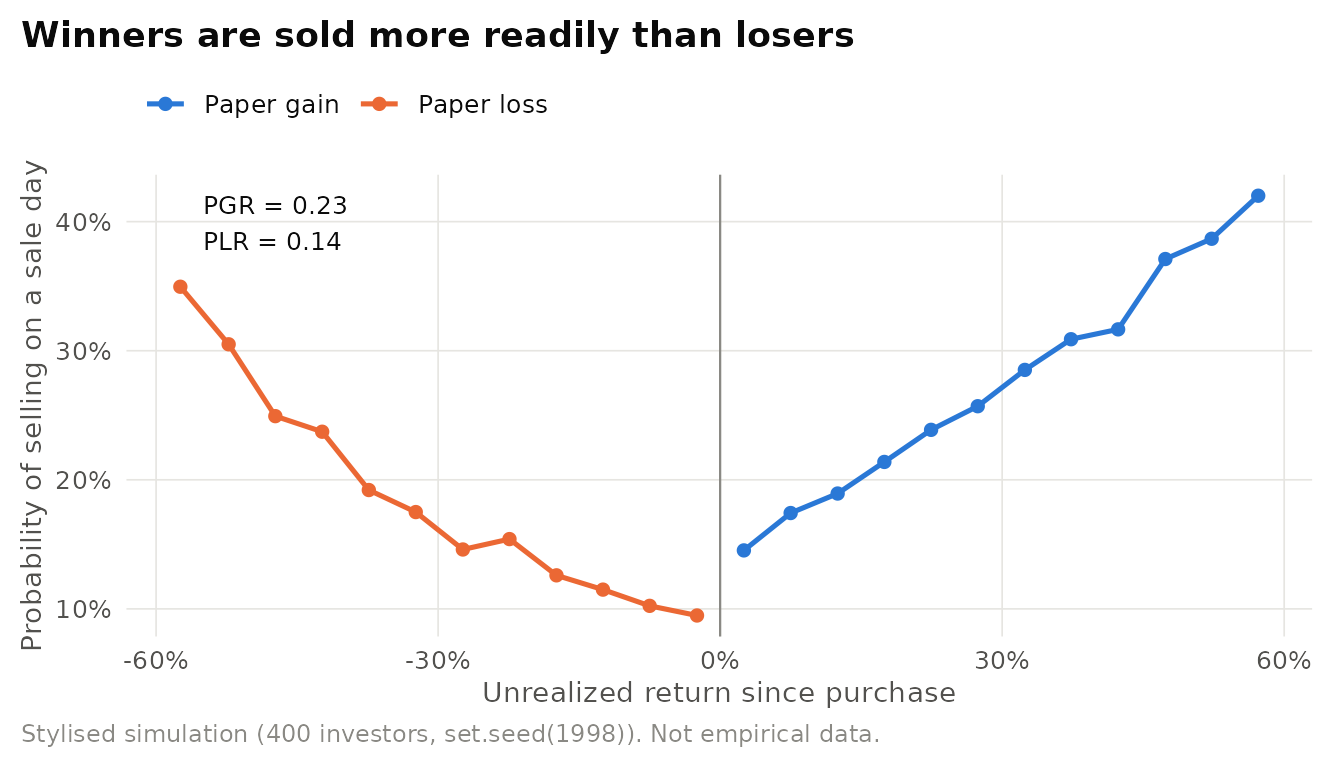
Figure 24.13: Stylised disposition effect in simulated trading data. The probability of selling a position on a sale day is plotted against its unrealized return since purchase. Selling rises with the size of the return in both directions and jumps at zero, so the proportion of gains realized (PGR) exceeds the proportion of losses realized (PLR). Illustrative simulation, not empirical data.

The effect is not confined to stock markets. Genesove and Mayer (2001) found that Boston condominium owners facing nominal losses in the 1990s set asking prices higher by 25-35% of the difference between the property’s expected selling price and their original purchase price, achieved higher selling prices by 3-18% of that difference, and sold much more slowly than other sellers. The list price effects were about twice as large for owner-occupants as for investors but held for both. In a controlled experimental market where the expected returns of assets were known, M. Weber and Camerer (1998) also found that participants sold more winners than losers.

Is the disposition effect really prospect theory? The textbook explanation has been challenged on theoretical and empirical grounds. N. Barberis and Xiong (2009) modelled a prospect-theory investor carefully and found that when preferences are defined over annual gains and losses, the model often predicts the opposite of the disposition effect. A loss-averse investor buys a stock only if its expected return is high. After a gain she moves away from the kink in the value function and is willing to hold more, while after a loss she moves toward the kink, where loss aversion bites hardest, and reduces her position. The disposition effect emerges more reliably if utility is derived from realizing gains and losses, a preference that N. Barberis and Xiong (2009) call realization utility. Kaustia (2010) showed that the propensity to sell jumps at a zero return but is approximately constant over a wide range of losses and constant or increasing over gains, a pattern hard to reconcile with the curvature of the value function. Ben-David and Hirshleifer (2012) found that selling is V-shaped in past returns: investors are more likely to sell large winners and large losers than small ones, which suggests belief-based trading rather than a preference for realizing gains. Imas (2016) added a twist: after a realized loss people take less risk, but after a paper loss they take more, so the act of realization itself changes the reference point. The consensus is that the disposition effect is a robust empirical regularity whose cause is more likely realization utility, regret, or beliefs than the S-shaped value function alone.

Table 24.15 presents the explanations for the disposition effect.

Table 24.15: Explanations for the disposition effect.

Explanation	Core idea	Key evidence or source
Prospect theory value function	Concavity above and convexity below the purchase price	Shefrin & Statman (1985), but see Barberis & Xiong (2009)
Realization utility	Investors derive utility from the act of realizing a gain or loss	Barberis & Xiong (2009)
Regret and self-justification	Selling a loser confirms a mistake	Shefrin & Statman (1985)
Beliefs in mean reversion	Investors expect losers to rebound and winners to fall back	Odean (1998) rules out several rational motives, Ben-David & Hirshleifer (2012)
Break-even seeking	Paper losses invite risk taking to get back to the reference point	Thaler & Johnson (1990), Imas (2016)
Tax considerations	Realizing losses reduces tax liability	Predicts the opposite pattern, so it cannot explain the effect

Brokerage and wealth-management practice. The disposition effect has practical consequences for retail investors, who sell winners that keep winning and hold losers that keep losing, and for the firms that serve them. Practices that weaken the effect include automatic rebalancing rules, pre-set stop-loss and take-profit rules decided before positions move, year-round tax-loss harvesting that reframes a realized loss as a tax gain, and statements that report portfolio-level rather than position-level returns, which makes the purchase price of each holding less salient. In real estate, agents can use the evidence of Genesove and Mayer (2001) to anticipate that sellers facing nominal losses will over-price and stay on the market longer, and price-setting conversations can shift the reference point from the purchase price to recent comparable sales.

24.9 Further Applications

Few theories have travelled as far as prospect theory. Table 24.16 maps its components to application domains, and the subsections that follow discuss the most important ones for business and policy. Each application relies on a different part of the theory, which is worth keeping in mind: evidence for one component (for example, probability weighting in lottery markets) is not evidence for another (for example, loss aversion in labour supply).

Table 24.16: Prospect theory applications by domain.

Domain	Component of the theory	Signature prediction	Illustrative evidence
Pricing	Reference dependence, loss aversion	Surcharges and price increases hurt more than equivalent discounts and decreases help	Thaler (1980), Hardie et al. (1993)
Promotions and messaging	Framing, loss aversion	Loss-framed messages can motivate more than gain-framed ones	Ganzach & Karsahi (1995)
Insurance	Probability weighting, loss aversion	Over-insurance of modest risks, preference for low deductibles	Johnson et al. (1993), Sydnor (2010)
Lotteries and skewed assets	Overweighting of small probabilities	Demand for and overpricing of lottery-like payoffs	Barberis & Huang (2008)
Asset pricing	Myopic loss aversion, narrow framing	High equity premium, non-participation	Benartzi & Thaler (1995), Barberis et al. (2001)
Trading	Purchase price as reference point	Disposition effect	Odean (1998), Genesove & Mayer (2001)
Labour and effort	Expectations and goals as reference points	Bunching at targets, effort responds to expectations	Abeler et al. (2011), Allen et al. (2017)
Tax compliance	Loss aversion around a zero balance due	More avoidance when a payment is owed than when a refund is due	Engström et al. (2015), Rees-Jones (2018)
Health and energy	Goal framing, loss-framed incentives	Deposit contracts and loss-framed incentives can outperform equivalent rewards	Patel et al. (2016), Halpern et al. (2015)
Negotiation and politics	Reference dependence, reflection effect	Loss frames make negotiators tougher and leaders more risk seeking	Neale & Bazerman (1985), Levy (1992)

24.9.1 Pricing and reference prices

The idea that customers code prices relative to a reference point is the most direct business application of the theory. R. Thaler (1980) noted that the credit card industry preferred that any price difference between card and cash payments be described as a “cash discount” rather than a “credit card surcharge”, anticipating that a surcharge would be coded as a loss. Reference prices also govern perceptions of fairness: customers accept price increases that pass on higher costs but regard increases that exploit a surge in demand as unfair, because the previous price acts as a reference transaction (Kahneman, Knetsch, and Thaler 1986). In scanner-panel data, Hardie, Johnson, and Fader (1993) modelled brand choice with reference-dependent utility and found evidence of loss aversion with respect to the reference brand’s price and quality: consumers were more responsive to being worse off than to being better off relative to the brand they had last bought. Kalyanaram and Winer (1995) summarized the empirical generalizations of reference price research, beginning with the finding that reference prices significantly affect demand.

Framing price differences. The same price structure can be presented as a surcharge (the base price is the low price, and some customers pay extra) or as a discount (the base price is the high price, and some customers pay less). Prospect theory predicts that customers who end up paying the higher price will feel worse under the surcharge frame, and customers who pay the lower price will feel only mildly better under the discount frame. Airlines, utilities, and payment providers face this choice every time they differentiate prices by channel, time, or payment method. Combined with mental accounting, the theory also predicts that many small fees, each coded as a separate loss, will feel worse than one all-inclusive price (Mental accounting (Section 23.5)). The managerial implication is not always to choose the discount frame: a surcharge may be the more effective way to steer customers toward a cheaper channel precisely because it is more aversive, but it carries reputational costs that the discount frame avoids.

24.9.2 Promotions and marketing messages

Loss framing is a standard tool in promotional copy (“Don’t miss out”, “You are losing $X a month”). The evidence is supportive but more nuanced than practitioners assume. In a field experiment with credit card holders, Ganzach and Karsahi (1995) found that a message emphasizing what customers lose by not using their card produced more subsequent card use than a message emphasizing what they gain by using it. Goal-framing effects of this kind are, however, distinct from risky-choice framing and attribute framing, and they vary in size and even direction across settings (Levin, Schneider, and Gaeth 1998). Firms should treat loss framing as a hypothesis to test in controlled experiments.

24.9.3 Insurance, lotteries, and skewed assets

Insurance and lotteries are where probability weighting does most of its work. Overweighting of small probabilities makes people willing to pay well above expected value both to eliminate a small chance of loss (insurance) and to buy a small chance of a large gain (lotteries), the two “low probability” cells of the fourfold pattern. Reviewing three decades of applications in economics, N. C. Barberis (2013) highlighted insurance and finance as domains in which the theory helps to explain facts that are otherwise hard to account for. Sydnor (2010) studied deductible choices in home insurance and found that most customers chose low deductibles despite premiums far above the expected value of the additional coverage, a level of risk aversion over modest stakes that a standard expected-utility model can fit only with implausible parameters. In financial markets, N. Barberis and Huang (2008) showed that investors with cumulative prospect theory preferences overvalue securities with positively skewed, lottery-like returns, which can make such securities earn low average returns, and N. Barberis, Mukherjee, and Wang (2016) found that stocks whose past return distributions are more attractive under prospect theory tend to have lower subsequent returns.

Insurance deductibles and extended warranties. Low deductibles, extended warranties, and add-on protection plans sell well even when their price is many times the expected cost of the risk they cover (Sydnor 2010). Prospect theory offers two reasons. Small probabilities of loss are overweighted, and paying a deductible after a claim is coded as an additional, salient loss on top of the damage itself. Insurers can use this insight responsibly, for example by offering a low-deductible option alongside clear information on expected claim costs, or exploitatively, by pricing low-deductible options far above cost. Regulators and consumer advocates increasingly treat the second as a consumer-protection issue.

24.9.4 Labour and tax compliance

Reference points shape how people respond to taxes. In Sweden, taxpayers receive a preliminary statement showing whether they owe money or are due a refund. Using data on 3.6 million Swedish taxpayers and a regression kink and discontinuity design, Engström et al. (2015) found strong causal effects of a preliminary deficit on the probability of claiming deductions, and concluded that calibrating withholding so that most taxpayers receive refunds would increase compliance. In US tax returns, Rees-Jones (2018) estimated that taxpayers facing a payment on tax day reduce their tax liability by $34 more than taxpayers owed a refund. In both studies, the reference point is a zero balance due, and owing money is coded as a loss. Labour-market applications, including effort provision, daily labour supply, and job search, are discussed in Reference-dependent preferences.

24.9.5 Sports

Sport provides unusually clean tests because outcomes are precisely measured and reference points are institutionally defined: par in golf (Pope and Schweitzer 2011), round-number finishing times in marathons (E. J. Allen et al. 2017), and betting lines in football (Card and Dahl 2011). Sports settings also show that reference dependence survives expertise, high stakes, and competition, which answers the common objection that behavioural anomalies disappear among experienced professionals operating in markets.

24.9.6 Public policy and health messaging

Rothman and Salovey (1997) proposed an influential refinement of goal framing for health communication. Behaviours that prevent illness (sunscreen, exercise) are perceived as low risk, so gain-framed messages should be more persuasive. Behaviours that detect illness (screening) carry the risk of an unwelcome discovery, so loss-framed messages should be more persuasive, by analogy with the risk seeking that prospect theory predicts in the loss domain. Early evidence was encouraging: women who read pamphlets emphasizing the negative consequences of not performing breast self-examination showed more favourable attitudes and behaviour than those who read pamphlets emphasizing the benefits of performing it (Meyerowitz and Chaiken 1987). Meta-analytic evidence is more sobering: across disease-prevention studies, the average difference between gain-framed and loss-framed messages is small (O’Keefe and Jensen 2007).

Loss aversion has had more consistent success in the design of incentives than of messages. In a randomized trial with overweight and obese adults, Patel et al. (2016) compared financial incentives for meeting a daily step goal that were framed as gains, as lotteries, or as losses (money allocated in advance and taken away for each day the goal was missed). Only the loss-framed incentive increased goal attainment significantly relative to control. In a large trial of smoking-cessation programmes, Halpern et al. (2015) found that deposit contracts, in which participants put their own money at risk, were accepted by fewer people than reward programmes, but were more effective among those who accepted them, illustrating the trade-off between the motivational power of loss-based incentives and their unattractiveness at enrolment. Volpp et al. (2008) found that both deposit contracts and lottery-based incentives produced more weight loss than a control condition during a weight-loss intervention.

Loss-framed energy and health messages. In a classic quasi-experiment, home energy auditors were trained to communicate their findings vividly and to frame the potential savings as money the household was losing through leaks and poor insulation. Homeowners who received these audits were more likely to apply for retrofit programmes than homeowners who received standard audits (Gonzales, Aronson, and Costanzo 1988). Utilities and health insurers have since used similar framing alongside other behavioural levers such as social comparisons (Social norms (Section 22.5)), and loss-framed incentive designs such as pre-funded wellness accounts draw directly on Patel et al. (2016). The lesson from the meta-analytic evidence (O’Keefe and Jensen 2007) is that loss frames are not a universal improvement: they work best when the behaviour involves risk or uncertainty and when the reference point is clear to the audience.

24.9.7 Negotiation and politics

In a negotiation, what one side gives up is coded as a loss and what it receives as a gain, so concessions loom larger to the conceder than to the recipient. Neale and Bazerman (1985) showed that framing changes bargaining: negotiators instructed to think about their outcomes as gains were more concessionary and completed more transactions than negotiators instructed to think about them as losses. In international relations, Levy (1992) argued that prospect theory explains why states and leaders accept large risks to avoid losses (for example, to recover lost territory or status) that they would not accept to make equivalent gains, while noting the analytical difficulty of identifying the reference point of a state.

Bringing prospect theory to a new domain.

• Specify the component. State whether the prediction rests on reference dependence, loss aversion, diminishing sensitivity, or probability weighting.
• Identify the reference point ex ante. Use institutional features (par, purchase price, zero balance due, quota) or measured expectations.
• Find a discontinuity. Reference points create kinks and notches. Bunching and regression discontinuity designs exploit them.
• Rule out alternatives. Inertia, attention, transaction costs, beliefs, and the range of outcomes can all mimic loss aversion.
• Sample hypothesis. H1. Customers who receive a loss-framed renewal reminder (“You will lose your saved settings”) will renew at a higher rate than customers who receive an equivalent gain-framed reminder, and the effect will be larger among customers with higher usage (a stronger sense of ownership).

24.10 Replication and Robustness

Prospect theory is built on demonstrations that are cheap to run, which makes it unusually easy to test whether its foundations replicate. The answer is encouraging. Ruggeri et al. (2020) repeated the original 1979 choice problems with 4,098 participants in 19 countries and 13 languages, adjusting only the currency and amounts to local conditions and requiring every participant to answer every item. The results replicated for 94% of items, with some attenuation of effect sizes, and 12 of 13 theoretical contrasts replicated, with complete replication in some countries. The authors also documented meaningful heterogeneity between countries and within individuals. The framing effect in the “Asian disease” problem (Tversky and Kahneman 1981) was among the effects that replicated in the first Many Labs project (R. A. Klein et al. 2014).

The picture is more mixed for the theory’s extensions and field applications. Table 24.17 summarises the state of the evidence as of this writing.

Table 24.17: What replicates and what does not: the state of the evidence on prospect theory.

Claim	Status	Evidence
Certainty, reflection, and isolation effects in described lotteries	Replicates	Ruggeri et al. (2020): 94% of items and 12 of 13 contrasts, with some attenuation
Risky-choice framing (Asian disease)	Replicates	Many Labs 1 (Klein et al., 2014)
Loss aversion on average	Replicates, smaller than 2.25	Meta-analytic mean 1.955 (Brown et al., 2024)
Loss aversion as a universal constant	Does not hold	Context and range effects, small stakes, exchange goods (Walasek & Stewart, 2015, Harinck et al., 2007, Novemsky & Kahneman, 2005)
Overweighting of rare events	Holds for description, often reverses for experience	Hertwig et al. (2004)
Expectations as reference points	Mixed	Abeler et al. (2011) versus Gneezy et al. (2017) and Heffetz & List (2014)
Daily income targeting by taxi drivers	Contested	Camerer et al. (1997) versus Farber (2008, 2015), Thakral & Tô (2021)
Myopic loss aversion	Replicates in experiments, including with professionals	Gneezy & Potters (1997), Haigh & List (2005)
Disposition effect as an empirical regularity	Robust	Odean (1998), Genesove & Mayer (2001), Weber & Camerer (1998)
Disposition effect caused by the S-shaped value function	Doubtful	Barberis & Xiong (2009), Kaustia (2010), Ben-David & Hirshleifer (2012)
Reference dependence in high-stakes field settings	Robust	Pope & Schweitzer (2011), Allen et al. (2017), Card & Dahl (2011)

Three lessons emerge. First, the qualitative patterns that motivated prospect theory are among the most reliable findings in the behavioural sciences. Second, quantitative parameters, especially the loss aversion coefficient, vary with people, tasks, and contexts, so a single “true” value should not be imported uncritically into applied models. Third, the theory’s empirical success in a new domain depends on how well the reference point is specified, which is a modelling choice rather than a prediction of the theory itself (N. C. Barberis 2013, O’Donoghue and Sprenger 2018).

Importing parameter values without checking the context. Simulations and structural models often plug in \(\alpha = 0.88\), \(\lambda = 2.25\), and \(\gamma = 0.61\) as if they were universal constants. They are median estimates from one study of described lotteries. When results depend on these values, report sensitivity analyses over plausible ranges, for example \(\lambda\) from about 1.5 to 2.5, and prefer estimates from populations and tasks similar to the application.

24.11 Chapter Summary

• Expected utility theory remains the normative benchmark, but the Allais and Ellsberg paradoxes and Rabin’s calibration theorem show that it cannot describe how people actually evaluate risk, especially over modest stakes (Allais 1953, Ellsberg 1961, Rabin 2000).
• Prospect theory replaces final wealth with gains and losses relative to a reference point, and combines a value function (diminishing sensitivity and loss aversion) with decision weights (overweighting of small probabilities) (Kahneman and Tversky 1979).
• Cumulative prospect theory applies weights to cumulative probabilities, preserving dominance and generating the fourfold pattern of risk attitudes. Its median parameters, \(\alpha = \beta = 0.88\), \(\lambda = 2.25\), \(\gamma = 0.61\), and \(\delta = 0.69\), are useful defaults, not constants (Tversky and Kahneman 1992).
• Loss aversion is real on average, with a meta-analytic mean coefficient near 2, but it is moderated by stakes, goods, experience, and the range of outcomes (A. L. Brown et al. 2024, Mrkva et al. 2020, Walasek and Stewart 2015).
• Reference points can be the status quo, expectations, goals, or salient numbers. Expectation-based models discipline the choice but have mixed experimental support (Kőszegi and Rabin 2006, Abeler et al. 2011, Gneezy et al. 2017).
• Status quo bias, myopic loss aversion, and the disposition effect are the theory’s most consequential applications, with large effects on retirement saving, asset prices, and trading (Madrian and Shea 2001, Benartzi and Thaler 1995, Odean 1998).
• The original choice patterns replicate across 19 countries (Ruggeri et al. 2020). The theory’s weakest point is not its foundations but the specification of the reference point in each new application.

Table 24.18 presents the comparison of expected utility, prospect theory, cumulative prospect theory, and expectation-based reference-dependent preferences.

Table 24.18: Comparison of expected utility, prospect theory, cumulative prospect theory, and expectation-based reference-dependent preferences.

Feature	Expected utility	Prospect theory (1979)	Cumulative prospect theory (1992)	Expectation-based reference dependence (2006)
Carriers of value	Final wealth	Gains and losses	Gains and losses	Consumption plus gains and losses
Reference point	None	Usually the status quo, unspecified	Usually the status quo, unspecified	Recent rational expectations (stochastic)
Risk attitude from	Curvature of utility	Value function and decision weights	Value function and rank-dependent weights	Consumption utility and gain-loss utility
Probability treatment	Linear	Decision weights on individual probabilities	Weights on cumulative probabilities	Usually linear
Loss aversion	No	Yes	Yes (lambda)	Yes (lambda), relative to expectations
Stochastic dominance	Satisfied	Can be violated	Satisfied	Satisfied in standard applications
Signature prediction	Consistent preferences across common consequences	Certainty, reflection, isolation effects	Fourfold pattern of risk attitudes	Surprises, not outcomes, drive gain-loss feelings
Key source	von Neumann & Morgenstern (1944)	Kahneman & Tversky (1979)	Tversky & Kahneman (1992)	Kőszegi & Rabin (2006)

24.12 Discussion Questions

1. Rabin’s calibration theorem is sometimes described as the strongest argument for prospect theory. Explain the theorem in your own words. Does it show that expected utility is wrong, or only that wealth is the wrong argument of the utility function?
2. Choose a pricing decision in a firm you know (a price increase, a new fee, a change in subscription terms). Identify at least three candidate reference points customers could use, and design a field experiment that would reveal which one drives their response.
3. The debate over loss aversion has moved from whether losses loom larger than gains to when and for whom. Propose a study that would distinguish loss aversion from inertia in a setting of your choice.
4. Using Figure 24.12 and the evidence on myopic loss aversion, argue for or against a regulation that would require retirement plan providers to show long-horizon return distributions by default. Whose interests would such a rule serve?
5. The disposition effect is robust, but its cause is debated. What data from a brokerage platform would allow you to distinguish realization utility, beliefs in mean reversion, and the S-shaped value function as explanations?
6. Loss-framed incentives (deposit contracts, claw-back bonuses) can be more effective than equivalent rewards but are less attractive at enrolment and can feel unfair. Under what conditions should an employer or health insurer use them?

24.13 Further Reading

• Kahneman and Tversky (1979): the original paper. Read the choice problems first, then the model, and notice how much of later research is foreshadowed in the discussion of editing.
• Tversky and Kahneman (1992): the cumulative version, with the parameter estimates that became the field’s defaults.
• Wakker (2010): the definitive technical treatment of prospect theory for risk and ambiguity, with careful attention to measurement.
• N. C. Barberis (2013): an accessible assessment of thirty years of applications in economics, especially finance and insurance.
• O’Donoghue and Sprenger (2018): a rigorous handbook review of reference-dependent preferences, including the Kőszegi-Rabin model and the field evidence.
• A. L. Brown et al. (2024): the most comprehensive meta-analysis of loss aversion estimates. Pair it with Gal and Rucker (2018b) and Mrkva et al. (2020) for the debate.
• Ruggeri et al. (2020): a multinational replication of the original problems and a model of how to test a classic finding at scale.
• DellaVigna (2009): a survey of field evidence in psychology and economics, with an extensive section on reference dependence.