16 Finance and Corporate Policy

In 1976 a small fund company in Pennsylvania launched a mutual fund that promised never to beat the market. It would simply hold the stocks in the S&P 500 in proportion to their market value and charge very little for doing so. The offering raised far less than its sponsors had hoped, and many in the industry regarded it as a curiosity. Half a century later, index funds are among the largest pools of capital in the world, and the firm that launched that first retail index fund, Vanguard, is one of the largest asset managers anywhere. Why would investors deliberately give up the chance to outperform? Why do cash-rich companies borrow billions of dollars they do not seem to need? Why did a hedge fund whose partners included two Nobel laureates nearly collapse in 1998, and why did the shares of a struggling video-game retailer rise more than tenfold in a few weeks of January 2021?

Each puzzle sits on a different branch of financial theory, but they share a root. Finance studies how people and firms trade claims on uncertain future cash flows, and almost every theory in the field is an answer to one of three questions. How should risk be priced? (portfolio theory and the capital asset pricing model). How much do prices reveal? (the efficient market hypothesis, the limits to arbitrage, and behavioural finance). How should a firm finance itself and what should it do with its cash? (the Modigliani-Miller theorems, the trade-off and pecking order theories, and free cash flow theory). This chapter develops all eight, with formal logic where it is standard and applications to investing and corporate policy. They build on Agency theory (Section 6.1), Information asymmetry (Section 8.1), and Signaling theory (Section 8.2), and the behavioural theories connect to Prospect theory (Section 24.2) and Heuristics and biases (Section 23.2) (Table 16.1).

Table 16.1: Chapter at a glance: theories of finance and corporate policy.

Theory	Core question	Level of analysis	Key source
Portfolio theory	How should an investor combine risky assets?	Investor / portfolio	Markowitz (1952)
Capital asset pricing model	Which risks earn a premium in equilibrium?	Asset / market	Sharpe (1964), Lintner (1965)
Efficient market hypothesis	How fully do prices reflect available information?	Market	Fama (1970)
Modigliani-Miller theorems	When does financing affect firm value?	Firm / market	Modigliani & Miller (1958, 1963)
Trade-off and pecking order	Why do firms choose the leverage they do?	Firm	Kraus & Litzenberger (1973), Myers (1984)
Free cash flow theory	Why can surplus cash destroy value?	Firm / manager	Jensen (1986)
Limits to arbitrage	Why can mispricing persist?	Arbitrageur / market	Shleifer & Vishny (1997)
Behavioral finance	How do investor psychology and sentiment shape prices?	Investor / market	Barberis & Thaler (2003)

16.1 Portfolio Theory

Core claim. Investors should evaluate an asset not by its own risk but by its contribution to the risk of the whole portfolio. Combining assets whose returns are imperfectly correlated reduces risk without sacrificing expected return, and rational investors choose among portfolios on the efficient frontier.

Origins. Economics and finance. Markowitz (1952) formulated mean-variance portfolio selection. Tobin (1958) added the separation theorem. Markowitz shared the 1990 Nobel Memorial Prize in Economic Sciences with Merton Miller and William Sharpe.

Level of analysis. Individual investor or institutional portfolio.

Key constructs. Expected return, variance, covariance, correlation, diversification, efficient frontier, global minimum-variance portfolio, tangency portfolio, Sharpe ratio.

Boundary conditions. Investors care only about the mean and variance of portfolio returns (returns are approximately normal or utility is quadratic), inputs are known or well estimated, and the investment horizon is a single period.

Related theories. CAPM, Myopic loss aversion (Section 24.7), Mental accounting (Section 23.5), Behavioral finance.

16.1.1 Origins and intellectual history

Before 1952, investment advice focused on picking good securities: identify the asset with the highest expected value and buy it. Markowitz (1952) observed that this rule cannot explain why prudent investors hold many securities rather than one. Diversification is rational only if investors also care about risk, and once they do, the right unit of analysis is the portfolio. Markowitz measured risk as the variance of portfolio returns, which depends on the covariances among assets. Tobin (1958) then showed that with a riskless asset, every investor should hold the same risky portfolio and adjust overall risk by mixing it with the riskless asset. This separation theorem bridged portfolio choice and equilibrium asset pricing.

16.1.2 Core logic and propositions

For a portfolio with weights \(w_i\) on \(N\) assets, expected return is a weighted average, but variance is not:

\[E[R_p] = \sum_{i=1}^{N} w_i \, E[R_i], \qquad \sigma_p^2 = \sum_{i=1}^{N} \sum_{j=1}^{N} w_i w_j \sigma_{ij}.\]

With two assets the variance becomes \(\sigma_p^2 = w^2 \sigma_1^2 + (1-w)^2 \sigma_2^2 + 2w(1-w)\rho_{12}\sigma_1\sigma_2\). Whenever the correlation \(\rho_{12}\) is below one, the portfolio’s standard deviation is less than the weighted average of the two standard deviations. That gap is the gain from diversification. For an equally weighted portfolio of \(N\) assets with average variance \(\bar{\sigma}^2\) and average covariance \(\overline{\text{cov}}\),

\[\sigma_p^2 = \frac{1}{N}\,\bar{\sigma}^2 + \left(1 - \frac{1}{N}\right)\overline{\text{cov}}.\]

As \(N\) grows, the first term vanishes but the second does not. Risk that is specific to individual assets (idiosyncratic risk) can be diversified away. Risk that assets share (systematic risk) cannot. Figure 16.1 plots this decomposition.

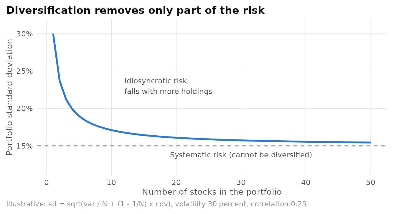
Figure 16.1: Illustrative diversification curve for an equally weighted portfolio. Each stock has 30 percent volatility and pairwise correlation 0.25. Idiosyncratic risk falls quickly as stocks are added, but systematic risk sets a floor.

The theory’s central propositions can be stated as follows.

• P1 (Risk is a portfolio property). The risk an asset adds to a portfolio depends on its covariance with the other holdings, not on its stand-alone variance.
• P2 (Diversification). Combining imperfectly correlated assets lowers portfolio variance for a given expected return. Only systematic risk remains in a large, well-diversified portfolio.
• P3 (Efficiency). A rational mean-variance investor holds a portfolio on the upper boundary of the feasible set: no other portfolio offers a higher expected return for the same variance.
• P4 (Separation). With a riskless asset, every mean-variance investor holds the same risky portfolio, the tangency portfolio with the highest Sharpe ratio \((E[R_p] - r_f)/\sigma_p\), and expresses risk tolerance only through the share invested in it (Tobin 1958).

16.1.3 Mechanism

Figure 16.2 builds the frontier from five simulated asset classes. The blue curve is the mean-variance frontier, whose upper arm is the efficient frontier. The orange capital allocation line runs from the riskless rate to the tangency portfolio and dominates every other point on the frontier.

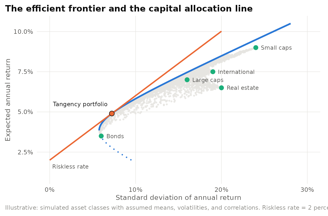
Figure 16.2: Illustrative efficient frontier for five simulated asset classes. Grey points are random long-only portfolios, the blue curve is the mean-variance frontier (short sales allowed), and the orange line combines the riskless asset with the tangency portfolio.

The lowest point on the frontier, the global minimum-variance portfolio, has a closed-form solution that requires no estimate of expected returns at all: \(w_{\text{GMV}} = \Sigma^{-1}\mathbf{1} / (\mathbf{1}'\Sigma^{-1}\mathbf{1})\), where \(\Sigma\) is the covariance matrix. The short computation below applies it to three illustrative asset classes.

# Illustrative covariance matrix of annual returns (volatility 6, 16, 24 percent)
Sigma3 <- matrix(c(0.0036, 0.0019, 0.0029,
                   0.0019, 0.0256, 0.0243,
                   0.0029, 0.0243, 0.0576),
                 nrow = 3, byrow = TRUE,
                 dimnames = list(c("Bonds", "Large caps", "Small caps"),
                                 c("Bonds", "Large caps", "Small caps")))
x <- solve(Sigma3, rep(1, 3))                # inverse(Sigma) times a vector of ones
w_gmv <- x / sum(x)                          # normalise so the weights sum to one
round(w_gmv, 3)

#>      Bonds Large caps Small caps 
#>      0.935      0.089     -0.025

sqrt(drop(t(w_gmv) %*% Sigma3 %*% w_gmv))    # volatility of the minimum-variance portfolio

#> [1] 0.0588677

The solution puts about 93 percent in bonds, a small long position in large caps, and a small short position in small caps. Its volatility is slightly below that of bonds alone, even though every other asset is riskier than bonds. That is Markowitz’s insight in miniature: a risky asset can lower portfolio risk when its correlation with the rest of the portfolio is low enough.

16.1.4 Evidence and extensions

Portfolio theory is normative, so its evidence concerns whether its prescriptions work. The gains from diversification are real and large, but the optimiser is very sensitive to its inputs: it loads heavily on the assets whose expected returns are most overestimated. DeMiguel, Garlappi, and Uppal (2009) compared fourteen optimised strategies with a naive rule that puts \(1/N\) in each asset and found that none consistently beat the naive rule out of sample across the datasets they studied, because estimation error offset the theoretical gains.

Is variance the right measure of risk? Mean-variance analysis treats upside and downside deviations symmetrically and assumes that the first two moments capture everything investors care about. Real return distributions have fat tails, and correlations tend to rise in crises, which is exactly when diversification is most needed. Behavioural evidence adds that investors weigh losses more heavily than gains (Kahneman and Tversky 1979, N. C. Barberis 2013), see Loss aversion (Section 24.4). The pragmatic response has been shrinkage estimators, factor risk models, and weight constraints, which keep Markowitz’s architecture while taming its sensitivity to inputs.

16.1.5 Applications in business

Concentration in employer stock: the Enron 401(k) accounts. The clearest violation of portfolio theory in household finance is holding a large share of retirement savings in one’s own employer, whose wages and stock share the same firm-specific risk. When Enron filed for bankruptcy in December 2001, many employees whose 401(k) accounts were heavily invested in company stock lost much of their retirement savings along with their jobs. The episode fed into later US reforms that gave plan participants the right to diversify out of employer stock.

16.1.6 Using the theory in research

Sample hypotheses.

• H1. Households with lower financial literacy hold less diversified portfolios, measured by the share of idiosyncratic variance in portfolio variance.
• H2. Employees hold more employer stock when the employer has recently outperformed (extrapolation), controlling for plan design.

Measures. Portfolio variance decomposition, number of effective holdings (inverse Herfindahl of weights), Sharpe ratio, tracking error, out-of-sample volatility.

Designs and data. Out-of-sample backtests with rolling estimation windows, household brokerage and pension records, administrative data on retirement plans, natural experiments from changes in default investment options.

Treating historical averages as expected returns. Plugging sample means into an optimiser produces portfolios that are extremely concentrated and unstable, because the optimiser chases estimation noise. Report out-of-sample performance, use shrinkage or factor models for inputs, and compare against the naive \(1/N\) and minimum-variance benchmarks before claiming that an optimised portfolio adds value.

16.2 Capital Asset Pricing Model

Core claim. In equilibrium, an asset’s expected return depends only on its beta, its sensitivity to the return on the market portfolio. Idiosyncratic risk earns no premium because investors can diversify it away.

Origins. Finance. Sharpe (1964) and Lintner (1965), building on Markowitz (1952) and Tobin (1958). Extended to multifactor models by Fama and French (1992) and Fama and French (1993).

Level of analysis. Individual asset within a market in equilibrium.

Key constructs. Market portfolio, beta, market risk premium, security market line, alpha, systematic versus idiosyncratic risk, factor premia.

Boundary conditions. Investors are mean-variance optimisers with common beliefs, can borrow and lend at the riskless rate, face no taxes or transaction costs, and hold the market portfolio of all risky assets.

Related theories. Portfolio theory, Efficient market hypothesis, Modigliani-Miller, Behavioral finance.

16.2.1 Origins and intellectual history

If every investor follows Markowitz and Tobin and all share the same beliefs, they all hold the same tangency portfolio. In equilibrium, that portfolio must be the market portfolio, because the supply of every asset must be held by someone. Sharpe (1964) and Lintner (1965) worked out the pricing implication independently, and related versions were developed by Jack Treynor and Jan Mossin. The result was the first general equilibrium model of risk and return, and it gave both investors and corporate managers a usable formula for the cost of capital.

16.2.2 Core logic and propositions

The CAPM states that the expected excess return on any asset is proportional to its beta:

\[E[R_i] = r_f + \beta_i \left( E[R_m] - r_f \right), \qquad \beta_i = \frac{\operatorname{Cov}(R_i, R_m)}{\operatorname{Var}(R_m)}.\]

An investor who holds the market portfolio cares about how a new asset changes the risk of that portfolio, which depends on the asset’s covariance with the market. An asset that falls when the market falls must offer a higher expected return. Purely idiosyncratic risk adds almost nothing and earns only the riskless rate.

• P1 (Only systematic risk is priced). Idiosyncratic volatility should not predict expected returns.
• P2 (Linearity). Expected returns are linear in beta, with intercept \(r_f\) and slope equal to the market risk premium.
• P3 (Zero alpha). In equilibrium the intercept \(\alpha_i\) in the regression of excess asset returns on excess market returns is zero for every asset.
• P4 (Market efficiency of the market portfolio). The market portfolio is mean-variance efficient. The CAPM is equivalent to this statement (Roll 1977).

16.2.3 Mechanism

The security market line (SML) in Figure 16.3 is the CAPM’s testable prediction. Assets above the line (positive alpha) would be bid up and assets below it sold until both return to the line. The orange points illustrate the pattern that empirical tests have repeatedly found: a line that is too flat, with low-beta portfolios earning more and high-beta portfolios earning less than the CAPM predicts (Fama and French 2004).

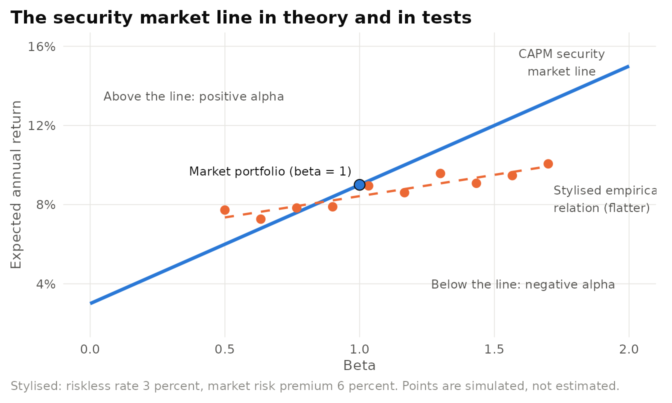
Figure 16.3: Stylised security market line. The blue line is the CAPM prediction. Orange points are stylised beta-sorted portfolios lying on a flatter line, the pattern reported in many empirical tests of the CAPM. Not empirical data.

16.2.4 Evidence and extensions

Early tests in the late 1960s and 1970s found that average returns rose with beta, but less steeply than the model predicts. Roll (1977) argued that the CAPM is not testable in practice, because the true market portfolio includes every risky asset and no index measures it. The decisive challenge came from Fama and French (1992): for US stocks from 1963 to 1990, beta had little power to explain average returns once firm size and the book-to-market ratio were included. Small firms and “value” firms with high book-to-market ratios earned more than their betas implied. Fama and French (1993) responded with a three-factor model in which returns load on the market, a size factor (SMB, small minus big), and a value factor (HML, high minus low book-to-market):

\[R_i - r_f = \alpha_i + b_i (R_m - r_f) + s_i \, \text{SMB} + h_i \, \text{HML} + \varepsilon_i .\]

Jegadeesh and Titman (1993) documented momentum, the tendency of recent winners to keep outperforming recent losers over three to twelve months, which the three-factor model does not explain. Carhart (1997) added a momentum factor for fund evaluation, and Fama and French (2015) added profitability and investment factors. Table 16.2 compares the main models.

Table 16.2: From the CAPM to multifactor models of expected returns.

Model	Risk factors	What it explains	Main limitation
CAPM (Sharpe 1964, Lintner 1965)	Market excess return	Why diversifiable risk is not rewarded	Flat empirical SML, size and value anomalies
Three-factor (Fama & French 1993)	Market, size (SMB), value (HML)	Size and value premia	Momentum, profitability
Four-factor (Carhart 1997)	Three factors plus momentum	Persistence in fund returns	Factors are empirical, not derived from theory
Five-factor (Fama & French 2015)	Market, size, value, profitability, investment	Profitability and investment patterns	Momentum, low-beta anomaly, short-term reversals

Risk, mispricing, or data mining? The size and value premia admit two readings. In the risk reading, small and value firms are exposed to distress or business-cycle risk that the market beta misses, so their premia are rational compensation. In the behavioural reading, investors extrapolate past growth and overprice glamour firms, so the premia reflect correctable mispricing (N. Barberis and Thaler 2003). A third concern is statistical. Harvey, Liu, and Zhu (2016) counted hundreds of proposed return factors and argued that, given the number of researchers searching the same data, a new factor should clear a t-statistic hurdle of about 3.0 rather than the conventional 2.0. The CAPM survives because it is simple and coherent, but few researchers regard it as an adequate empirical description of the cross-section of returns (Fama and French 2004).

16.2.5 Applications in business

In a large survey of chief financial officers, Graham and Harvey (2001) found that the CAPM was the most popular method for estimating the cost of equity, used by roughly three in four respondents. Investment managers use CAPM or multifactor alpha as the standard measure of skill, a practice that began with Jensen (1968).

Illustrative scenario: divisional hurdle rates. A diversified company has a regulated utility division and a biotechnology division and uses one company-wide cost of capital of 9 percent for all projects. Suppose the utility division’s asset beta is about 0.4 and the biotechnology division’s is about 1.5. With a riskless rate of 3 percent and a market risk premium of 6 percent, the CAPM implies hurdle rates of roughly 5.4 and 12 percent. The single company rate rejects good low-risk utility projects and accepts bad high-risk biotechnology projects. The remedy is divisional hurdle rates based on betas of comparable pure-play firms: the cost of capital belongs to the project, not the firm.

16.2.6 Using the theory in research

Sample hypotheses.

• H1. After controlling for market beta, firms with higher customer satisfaction earn lower subsequent returns because their cash flows are less risky.
• H2. The alpha of an investment strategy based on a new signal is not explained by the Fama-French five factors plus momentum.

Designs. Time-series regressions of portfolio excess returns on factors (alpha tests), Fama-MacBeth cross-sectional regressions of returns on characteristics and betas, portfolio sorts with out-of-sample periods.

Data. CRSP and Compustat for US equities, factor returns from Kenneth French’s data library, international equity databases, mutual fund return databases.

Mistaking a factor loading for an explanation. Showing that a strategy’s returns load on a factor does not explain why the factor earns a premium. Equally, an anomaly that disappears after controlling for factors may simply have been absorbed by a factor that is itself an unexplained anomaly. State whether a variable is meant to proxy for risk or for mispricing, and design a test that can tell the two apart.

16.3 Efficient Market Hypothesis

Core claim. In an efficient market, prices fully reflect available information, so no investor can earn returns in excess of fair compensation for risk by trading on that information.

Origins. Finance. Fama (1970) synthesised the theory and evidence, building on the random-walk literature. Fama shared the 2013 Nobel Memorial Prize with Lars Peter Hansen and Robert Shiller, one of the hypothesis’s leading critics.

Level of analysis. Market.

Key constructs. Information set, weak, semi-strong, and strong form efficiency, abnormal return, joint hypothesis problem, event study, anomaly.

Boundary conditions. Information is widely available, trading costs are low, and enough well-capitalised investors trade on information to keep prices close to fundamental value.

Related theories. Limits to arbitrage, Behavioral finance, Wisdom of the crowd (Section 30.5), Information asymmetry (Section 8.1).

16.3.1 Origins and intellectual history

Statisticians had long noticed that stock price changes look like a random walk. The insight behind the EMH is that this is what a well-functioning market should produce: if prices already reflect all predictable information, only new information moves them, and new information is by definition unpredictable. Fama (1970) organised the evidence around three information sets, summarised in Table 16.3.

Table 16.3: The three forms of market efficiency (following Fama, 1970).

Form	Information reflected in prices	Implication if true	Typical test
Weak form	Past prices and trading volume	Technical analysis cannot earn abnormal returns	Return autocorrelation, trading-rule backtests
Semi-strong form	All publicly available information	Fundamental analysis of public data cannot earn abnormal returns	Event studies of announcements
Strong form	All information, including private	Even insiders cannot profit	Returns to insider trades and professional managers

16.3.2 Core logic and propositions

Formally, a market is efficient with respect to an information set \(\Phi_t\) if the expected return conditional on that information equals the equilibrium expected return implied by some model of risk:

\[E\left[ R_{i,t+1} \mid \Phi_t \right] = E^{*}\left[ R_{i,t+1} \right], \qquad \text{so that} \quad E\left[ R_{i,t+1} - E^{*}[R_{i,t+1}] \mid \Phi_t \right] = 0 .\]

The abnormal return, the gap between realised and model-implied returns, should be unpredictable using \(\Phi_t\). This formulation exposes the joint hypothesis problem: every test of efficiency is also a test of the asset pricing model that defines \(E^{*}\). If returns appear predictable, either the market is inefficient or the risk model is wrong, and the data alone cannot say which (Fama 1970, 1998).

• P1 (No predictable abnormal returns). Abnormal returns are unpredictable from information in the relevant set.
• P2 (Rapid and unbiased adjustment). Prices react to new public information quickly and, on average, by the right amount, with no systematic drift or reversal.
• P3 (No persistent skill). Professional investors do not outperform risk-adjusted benchmarks after costs on a persistent basis.

16.3.3 Mechanism

The EMH rests on competition among informed traders, who trade until the price no longer offers a profit. Grossman and Stiglitz (1980) showed that if prices fully reflected all information, no one would have an incentive to pay for information, because they could learn it for free from prices. Yet if no one gathered information, prices could not reflect it. The resolution is an equilibrium degree of inefficiency: prices must be noisy enough to compensate informed traders for their costs. Figure 16.4 shows this loop.

Figure 16.4: Mechanism of informational efficiency and the Grossman-Stiglitz paradox. Informed trading makes prices informative, which lowers the profit from becoming informed. In equilibrium, noise keeps prices informative but imperfect, so information gathering remains just worth its cost.

16.3.4 Evidence and extensions

Event studies, which measure abnormal returns around announcements, show that prices typically react within minutes to earnings, merger bids, and macroeconomic releases, consistent with P2. On P3, Jensen (1968) and Carhart (1997) found that mutual funds on average do not beat risk-adjusted benchmarks after fees, and that the persistence that exists is concentrated among the worst performers.

Against this, researchers have catalogued anomalies. The best documented is post-earnings-announcement drift (PEAD): after a large positive earnings surprise, returns continue to drift upward for weeks, and after a large negative surprise they drift downward. Bernard and Thomas (1989) showed that the drift is difficult to explain as compensation for risk and concluded that it reflects a delayed price response, as if investors fail to incorporate the full implications of earnings news. Figure 16.5 sketches the pattern.

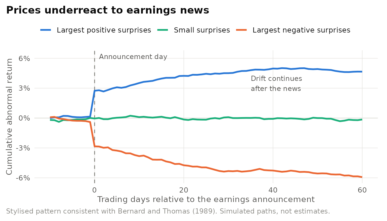
Figure 16.5: Stylised post-earnings-announcement drift. Cumulative abnormal returns jump at the announcement and then continue to drift in the direction of the surprise for about two months, a pattern inconsistent with complete and immediate adjustment. Not empirical data.

A second line of evidence concerns the level of prices rather than the predictability of returns. If a stock’s price is the expected present value of its future dividends, then the price \(p_t\) is a forecast of the ex post rational price \(p_t^{*} = \sum_{k \ge 1} D_{t+k}/(1+r)^k\). A rational forecast must be less volatile than the quantity it forecasts, so \(\operatorname{Var}(p_t) \le \operatorname{Var}(p_t^{*})\). Shiller (1981) found that US stock prices were far more volatile than this bound allowed, a result he interpreted as evidence that prices move too much to be justified by news about fundamentals.

Is the market efficient? The debate has matured rather than ended. Defenders emphasise that most anomalies are small, fragile, or explained by risk, that apparent overreactions are about as common as underreactions, and that active managers as a group do not beat passive benchmarks after costs (Fama 1998, Malkiel 2003). Critics reply that excess volatility, bubbles, and persistent anomalies show that prices can deviate from fundamental value for long periods (Shiller 1981, Shleifer 2000). A middle ground comes from McLean and Pontiff (2016): the returns to 97 published anomalies were about 26 percent lower out of sample and about 58 percent lower after publication. Some predictability was statistical bias, but much was real mispricing that informed traders then arbitraged away, as Grossman and Stiglitz would predict. The joint 2013 Nobel prize to Fama and Shiller captures the state of the field: markets are hard to beat, but prices are not always right.

16.3.5 Applications in business

Index funds and the rise of Vanguard. The most consequential application of the EMH is the index fund. P. A. Samuelson (1974) argued that few managers could be expected to beat the market and called for a low-cost fund that simply tracked a broad index. In 1976 John Bogle’s newly founded Vanguard launched the First Index Investment Trust, later renamed the Vanguard 500 Index Fund, to track the S&P 500. The initial offering raised only a small fraction of its target. Sharpe (1991) later stated the logic with great economy: before costs, the average actively managed dollar must earn the market return, so after costs it must underperform the average passive dollar. The argument requires only that outperformance be zero-sum before costs. French (2008) estimated that over 1980-2006 US investors spent about two thirds of one percent of the aggregate value of the market each year on fees, trading costs, and other expenses of active investing. Vanguard’s structure reinforced the strategy: the company is owned by its funds, and through them by fund shareholders, which aligns its incentives with low costs. The later growth of passive investing raises a new question: do markets remain informationally efficient if fewer investors gather information? That is the Grossman-Stiglitz paradox in practical form.

16.3.6 Using the theory in research

Sample hypotheses.

• H1. Post-earnings-announcement drift is stronger for firms with lower investor attention (fewer analysts, announcements on Fridays or busy news days).
• H2. Anomaly returns decline after the publication of the academic paper that documents them, and the decline is larger for anomalies that are cheaper to trade.

Designs. Event studies with market-model or factor-model abnormal returns, calendar-time portfolio regressions, difference-in-differences around changes in information access, tests of return predictability with out-of-sample validation.

Data. CRSP daily returns, I/B/E/S analyst forecasts and earnings surprises, news timestamps, SEC EDGAR filings.

Confusing “no free lunch” with “prices are right”. The EMH predicts that abnormal returns are unpredictable, not that prices equal fundamental value at every moment. A market can be hard to beat and still be wrong, because mispricing may be unpredictable in timing or too risky to correct. Conversely, finding a predictable return pattern does not prove inefficiency until risk and trading costs are ruled out. Always state the asset pricing model your test assumes.

16.4 The Modigliani-Miller Theorems

Core claim. In a perfect capital market, a firm’s value is determined by its real assets and investment policy, not by how it is financed. Capital structure and dividend policy are irrelevant. Once corporate taxes are introduced, debt adds value through the interest tax shield.

Origins. Economics and finance. Modigliani and Miller (1958) on capital structure, M. H. Miller and Modigliani (1961) on dividend policy, and Modigliani and Miller (1963) on corporate taxes. Modigliani received the Nobel Memorial Prize in 1985 and Miller in 1990.

Level of analysis. Firm in a capital market.

Key constructs. Firm value, leverage, cost of equity, cost of debt, weighted average cost of capital (WACC), homemade leverage, arbitrage, interest tax shield.

Boundary conditions. No taxes, bankruptcy costs, transaction costs, or information asymmetries, investors can borrow on the same terms as firms, and investment policy is held fixed.

Related theories. Trade-off and pecking order, Free cash flow theory, Agency theory (Section 6.1), Signaling theory (Section 8.2).

16.4.1 Origins and intellectual history

Before 1958, corporate finance was largely descriptive and institutional, and practitioners believed that a judicious amount of cheap debt lowered a firm’s cost of capital. Modigliani and Miller (1958) showed that this belief rests on an error. If investors can borrow and lend on the same terms as firms, any leverage a firm chooses can be undone or replicated by investors on their own account (homemade leverage). Two firms with identical assets but different capital structures must then have the same total value, or investors could earn a riskless profit by selling the overvalued firm and buying the undervalued one. The proof by arbitrage was itself a methodological innovation and became the template for modern asset pricing, including option pricing.

16.4.2 Core logic and propositions

The results are usually stated as three propositions and a tax correction. Let \(V_L\) and \(V_U\) be the values of levered and unlevered firms with the same assets, \(D\) and \(E\) the market values of debt and equity, \(r_A\) the return on assets, and \(r_D\) and \(r_E\) the returns on debt and equity.

• Proposition I (Value irrelevance). \(V_L = V_U\). The value of the firm is independent of its capital structure.
• Proposition II (Cost of equity). The expected return on equity rises linearly with the debt-to-equity ratio, exactly offsetting the apparent gain from cheaper debt:

\[r_E = r_A + \frac{D}{E}\left( r_A - r_D \right), \qquad \text{WACC} = \frac{E}{V} r_E + \frac{D}{V} r_D = r_A .\]

• Proposition III (Dividend irrelevance). Holding investment fixed, the split of earnings between dividends and retention does not affect value, because a dividend financed by issuing new shares transfers value from old to new shareholders one for one (M. H. Miller and Modigliani 1961).
• Tax correction. With a corporate tax rate \(\tau_c\) and permanent debt, interest payments are deductible and

\[V_L = V_U + \tau_c D, \qquad \text{WACC}_{\text{after-tax}} = r_A \left( 1 - \tau_c \frac{D}{V} \right),\]

so value rises with leverage (Modigliani and Miller 1963).

16.4.3 Mechanism

Figure 16.6 shows the propositions graphically. Without taxes, substituting cheap debt for expensive equity leaves the WACC unchanged because equity holders demand a higher return for the extra financial risk (in CAPM terms, leverage raises the equity beta). With taxes, the WACC falls as leverage rises.

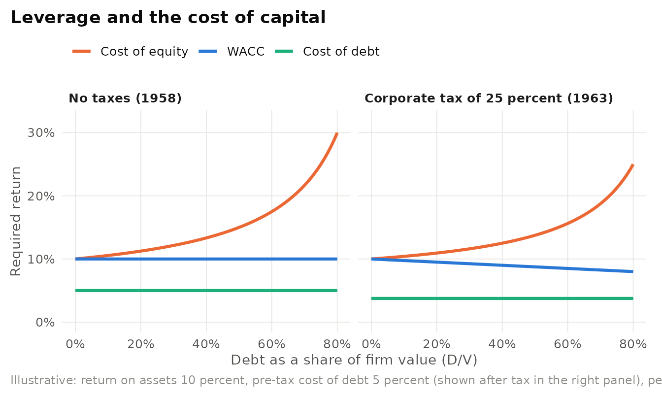
Figure 16.6: Illustrative Modigliani-Miller propositions. Without taxes, the cost of equity rises with leverage and the weighted average cost of capital stays flat. With a 25 percent corporate tax, the after-tax WACC declines as leverage rises because of the interest tax shield.

16.4.4 Evidence and extensions

The MM propositions are not empirical predictions in the usual sense. Their importance lies in what they imply about where to look. If financing matters, it must be because one of the assumptions fails. Table 16.4 maps the main research programs in corporate finance onto the assumptions they relax, which is why MM is often described as the foundation of the field rather than a description of it (Myers 2001).

Table 16.4: The Modigliani-Miller assumptions as a map of corporate finance.

MM assumption	What happens when it fails	Resulting theory	Key reference
No corporate taxes	Interest deductibility makes debt valuable	Tax shield, static trade-off	Modigliani & Miller (1963)
No costs of financial distress	Expected bankruptcy and distress costs offset tax benefits	Trade-off theory	Kraus & Litzenberger (1973)
Symmetric information	Equity issues signal overvaluation, internal funds are preferred	Pecking order theory	Myers & Majluf (1984)
No agency conflicts	Debt and payouts discipline managers with surplus cash	Free cash flow theory	Jensen (1986)
Investment policy fixed	Debt overhang causes underinvestment in good projects	Debt overhang	Myers (1977)
Prices equal fundamental value	Managers issue equity when it is overpriced	Market timing	Baker & Wurgler (2002)

Irrelevance as a benchmark or as a claim? Critics sometimes dismiss MM as unrealistic. Its defenders reply that unrealistic assumptions are the point: the theorems isolate the conditions under which financing could matter, and every later theory in this chapter is a precise answer to the question “which friction?” The remaining debate is quantitative: how large are the tax benefits of debt after personal taxes, and how large are expected distress costs? Those magnitudes have proved hard to pin down, as the next section shows.

16.4.5 Applications in business

Taxes and the Apple bond issue of 2013. In April 2013 Apple sold 17 billion dollars of bonds, at the time one of the largest corporate bond offerings on record, even though it held well over 100 billion dollars in cash and securities. A large share of that cash was held by foreign subsidiaries, and bringing it home would have triggered US taxes under the rules then in force. Borrowing at low interest rates to fund dividends and share repurchases let Apple return cash to shareholders without paying the repatriation tax, and the interest was tax deductible. The case illustrates the MM logic in reverse: financing decisions create value precisely when a friction, here the tax code, breaks the irrelevance conditions.

16.4.6 Using the theory in research

Sample hypotheses.

• H1. Exogenous increases in corporate tax rates lead firms to increase leverage, and the effect is larger for firms with fewer non-debt tax shields.
• H2. The equity beta of a firm rises with leverage as predicted by Proposition II after controlling for asset beta.

Designs. Natural experiments from tax reforms, staggered state tax changes, regression of equity betas on leverage, event studies of pure recapitalisations.

Data. Compustat fundamentals, CRSP returns, tax rate databases, bond issuance data (Mergent FISD).

Reading MM as “capital structure does not matter”. The theorems say that capital structure is irrelevant only under perfect markets, which makes them a checklist of reasons why it does matter. A second misuse is to apply Proposition II’s logic backward: a lower WACC from adding debt is not evidence of value creation unless the cost of equity has been adjusted for the higher financial risk.

16.5 Trade-off and Pecking Order Theories

Core claim. The static trade-off theory holds that firms choose a target leverage that balances the tax benefits of debt against the expected costs of financial distress. The pecking order theory holds that, because of information asymmetry, firms prefer internal funds to debt and debt to equity, so leverage is the cumulative result of past financing needs rather than a target.

Origins. Finance. Kraus and Litzenberger (1973) formalised the trade-off. Myers (1984) and Myers and Majluf (1984) developed the pecking order. Shyam-Sunder and Myers (1999) and Frank and Goyal (2003) set up the classic empirical contest.

Level of analysis. Firm.

Key constructs. Target leverage, interest tax shield, costs of financial distress, debt overhang, financing deficit, financial slack, adverse selection cost of equity, market timing.

Boundary conditions. Trade-off logic requires meaningful tax benefits and distress costs. Pecking order logic requires managers to know more than investors and to act in the interest of existing shareholders.

Related theories. Modigliani-Miller, Information asymmetry (Section 8.1), Signaling theory (Section 8.2), Free cash flow theory.

16.5.1 Origins and intellectual history

Once Modigliani and Miller (1963) showed that debt creates a tax shield, the obvious puzzle was why firms are not financed almost entirely with debt. Kraus and Litzenberger (1973) provided the standard answer in a state-preference model: debt creates tax savings in good states but deadweight bankruptcy costs in bad ones, so there is an interior optimum. Later work added the indirect costs of distress, such as lost customers and suppliers, and Myers (1977) identified debt overhang: a heavily indebted firm may forgo valuable projects because much of their payoff would go to creditors.

In his 1984 presidential address to the American Finance Association, published as “The Capital Structure Puzzle”, Myers (1984) argued that the trade-off theory fits the data poorly. Many highly profitable firms, which have the most taxable income to shield, borrow the least. He proposed instead a pecking order grounded in the asymmetric information model of Myers and Majluf (1984). If managers know more than investors about the value of the firm, they will be most willing to issue equity when it is overvalued. Investors understand this and treat an equity issue as bad news, so issuing equity is expensive for good firms. Internal funds avoid the problem entirely, and safe debt nearly does. The result is a financing hierarchy.

16.5.2 Core logic and propositions

The trade-off theory can be written as

\[V_L = V_U + \text{PV}(\text{interest tax shields}) - \text{PV}(\text{costs of financial distress}),\]

with the optimal debt level where the marginal tax benefit equals the marginal expected distress cost. The pecking order is usually tested with the financing deficit, the cash a firm must raise externally:

\[\text{DEF}_t = \text{DIV}_t + X_t + \Delta W_t + R_t - C_t, \qquad \Delta D_{it} = a + b_{\text{PO}} \, \text{DEF}_{it} + e_{it},\]

where DIV is dividends, \(X\) capital expenditure, \(\Delta W\) the increase in working capital, \(R\) the current portion of long-term debt, and \(C\) operating cash flow after interest and taxes. Under a strict pecking order, debt fills the deficit one for one, so \(a = 0\) and \(b_{\text{PO}} = 1\) (Shyam-Sunder and Myers 1999).

• P1 (Trade-off: target). Firms have target leverage ratios and adjust toward them.
• P2 (Trade-off: cross-section). Leverage rises with tax benefits and tangible assets and falls with distress costs, earnings volatility, and growth options.
• P3 (Pecking order: hierarchy). Firms use internal funds first, then debt, and issue equity only as a last resort.
• P4 (Pecking order: profitability). More profitable firms use less debt because they need less external finance.
• P5 (Pecking order: announcement effects). Announcements of equity issues are followed by negative abnormal returns, and the effect is larger when information asymmetry is greater.

16.5.3 Mechanism

Figure 16.7 shows the trade-off. The MM tax line rises without limit. Distress costs are negligible at low leverage and rise steeply as default becomes likely, so firm value peaks at an interior debt level.

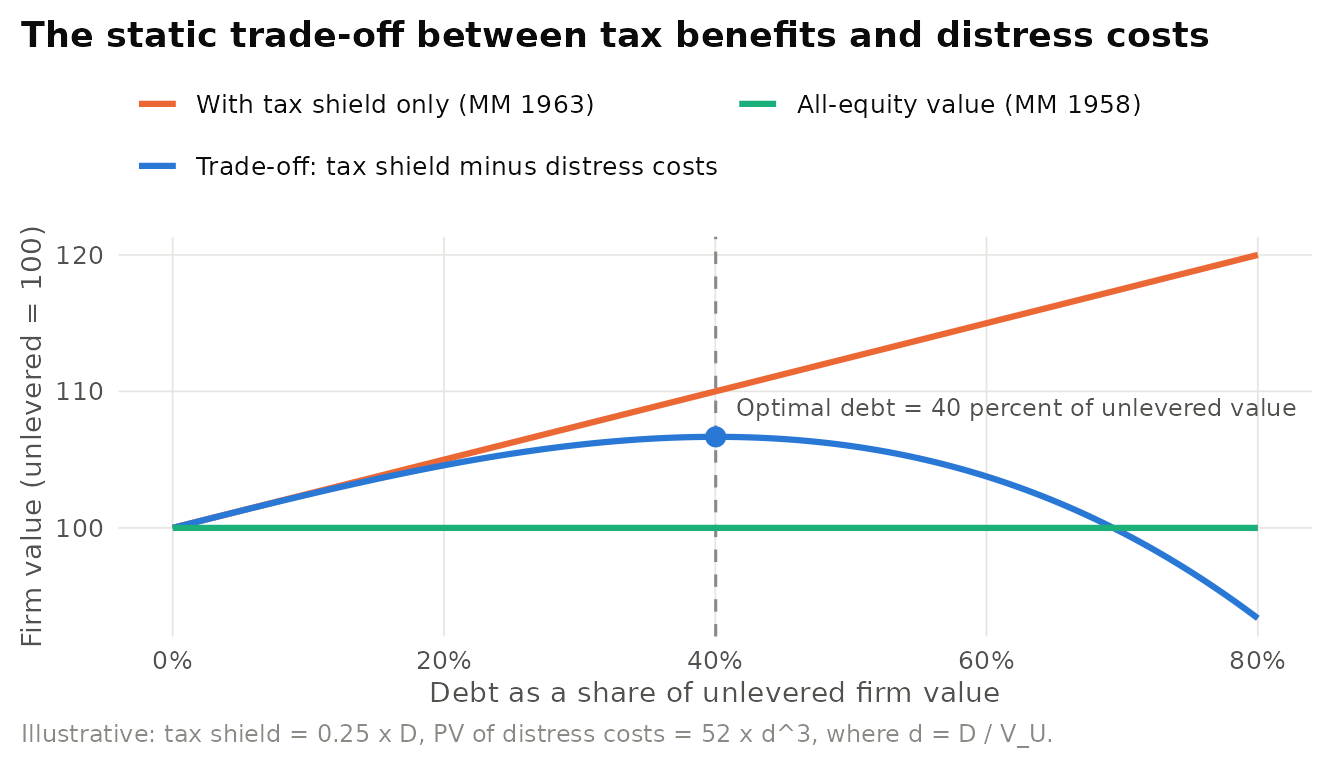
Figure 16.7: Illustrative static trade-off theory. The interest tax shield raises firm value linearly with debt, while the present value of financial distress costs rises with leverage. Firm value peaks at an interior optimum, marked by the dashed line.

Figure 16.8 summarises the pecking order mechanism. The cost of each source of funds rises with its sensitivity to managers’ private information.

Figure 16.8: Mechanism of the pecking order theory. Because managers know more than investors, securities whose value depends more on that private information carry a larger adverse selection discount. Firms therefore finance with internal funds first, then debt, and equity last. Financial slack relaxes the constraint.

16.5.4 Evidence and extensions

The two theories make sharply different predictions, summarised in Table 16.5. The empirical contest has run for four decades without a clear winner.

Table 16.5: Contrasting predictions of the static trade-off and pecking order theories.

Issue	Static trade-off	Pecking order	What the evidence suggests
Target leverage	Yes, firms adjust toward it	No well-defined target	Mixed: adjustment is slow, leverage is highly persistent
Profitability and leverage	Positive (more taxable income to shield)	Negative (less need for external funds)	Negative, favouring the pecking order
Response to financing deficit	Partial, depends on distance from target	Debt fills the deficit one for one	Strong for large mature firms, weak for small growth firms
Equity issuance	When leverage is above target	Rare, a last resort	Small growth firms issue equity often
Market reaction to equity issues	Neutral	Negative	Negative on average
Role of stock prices	None	None directly	Firms issue equity after price run-ups (market timing)

Shyam-Sunder and Myers (1999) found that for a sample of large, mature US firms, net debt issues tracked the financing deficit closely, which favoured the pecking order, and that standard target-adjustment tests had little power to distinguish the two theories. Frank and Goyal (2003) extended the test to a much broader sample of US firms and found that net equity issues tracked the deficit more closely than net debt issues. Small, high-growth firms, where information asymmetry and hence the pecking order should be strongest, issued the most equity. The pecking order fit best for large firms.

Two further findings complicate both theories. Lemmon, Roberts, and Zender (2008) showed that leverage is remarkably persistent, with most of its variation explained by a stable firm effect that standard determinants do not capture. M. Baker and Wurgler (2002) argued that firms issue equity when their market values are high relative to book and past market values, and that these market timing decisions have long-lasting effects on capital structure. In survey evidence, CFOs stressed financial flexibility and credit ratings, and few described their leverage target as strict (Graham and Harvey 2001).

Is there a capital structure theory at all? Myers (2001) concluded that there is no universal theory of the debt-equity choice, only conditional theories that work in different settings: trade-off logic for differences across industries, pecking order logic for the profitability effect and issue announcements, market timing for bursts of issuance in hot markets. A further critique is econometric: leverage ratios are mechanically mean-reverting, so finding “adjustment toward a target” does not by itself confirm the trade-off theory (Shyam-Sunder and Myers 1999).

16.5.5 Applications in business

Leverage decisions in practice. Firms in the same economy choose strikingly different capital structures, and the differences line up with trade-off logic. Regulated utilities and real estate investment trusts, whose cash flows are stable and whose assets are tangible and redeployable, routinely carry high leverage. Technology and biotechnology firms, whose value lies in growth options and intangible assets that would lose much of their value in distress, typically carry little net debt, and many hold large cash balances. Within those broad patterns, pecking order and timing behaviour are easy to observe. Announcements of seasoned equity offerings are, on average, followed by negative stock price reactions, consistent with Myers and Majluf (1984). Conversely, firms whose shares have run up issue equity opportunistically. In 2021, after the run-up in their share prices described in the Behavioral finance section, GameStop and AMC Entertainment both sold new shares through at-the-market offerings, using a high stock price to raise capital and reduce debt, which is market timing in the sense of M. Baker and Wurgler (2002).

16.5.6 Using the theory in research

Sample hypotheses.

• H1. The negative relation between profitability and leverage is stronger for firms with greater information asymmetry (fewer analysts, more intangible assets).
• H2. Firms issue more equity when their market-to-book ratio is high relative to its historical average, controlling for investment opportunities.

Measures. Book and market leverage, financing deficit, market-to-book ratio, asset tangibility, marginal tax rates, distance to default, analyst forecast dispersion as a proxy for information asymmetry.

Designs. Partial adjustment models of leverage, financing deficit regressions, event studies of security issues, natural experiments from tax and bankruptcy law changes, surveys of CFOs.

Treating every cross-sectional correlation as a test of one theory. Profitability, size, tangibility, and growth opportunities are related to leverage under several theories at once, often with the same sign. A negative profitability coefficient is consistent with the pecking order but also with mean reversion in leverage and with agency explanations. Specify which prediction is unique to the theory you are testing, and use settings where the theories diverge.

16.6 Free Cash Flow Theory

Core claim. When a firm generates more cash than it can invest in positive net present value projects, self-interested managers tend to waste the surplus on low-return growth rather than return it to shareholders. Debt, payouts, and the market for corporate control reduce these agency costs.

Origins. Finance and organisational economics. Jensen (1986), building on the agency framework of Jensen and Meckling (1976).

Level of analysis. Firm and top management.

Key constructs. Free cash flow, empire building, agency costs of equity, debt as a bonding device, payout policy, leveraged buyout, market for corporate control.

Boundary conditions. Firms have substantial cash flows and limited growth opportunities, and managerial incentives are imperfectly aligned with shareholders’. The theory has least force for young, high-growth firms with more good projects than cash.

Related theories. Agency theory (Section 6.1), Stewardship theory (Section 6.2), Upper echelons theory (Section 6.4), Modigliani-Miller.

16.6.1 Origins and intellectual history

Jensen’s 1986 paper applied the agency framework of Jensen and Meckling (1976) to a specific question: what happens to cash a firm does not need? He defined free cash flow as cash flow in excess of that required to fund all projects with positive net present value at the relevant cost of capital. Managers, he argued, want firms to grow beyond their optimal size because size brings power, status, and pay, and free cash flow fuels that growth. Jensen used the theory to explain the takeovers and leveraged buyouts of the 1980s, and he pointed to the oil industry, where high prices in the late 1970s generated large cash flows that many companies reinvested in exploration and diversification even as the returns to such investment declined (Jensen 1986).

16.6.2 Core logic and propositions

• P1 (Overinvestment). Firms with high free cash flow and poor investment opportunities overinvest, for instance in diversifying acquisitions, and these investments earn low returns.
• P2 (Debt as bonding). Debt commits managers to pay out future cash flows, reducing the cash available for waste. Unlike a promise to pay dividends, debt payments are enforceable through bankruptcy.
• P3 (Payouts). Increases in dividends and repurchases by firms with free cash flow problems are good news for shareholders. Cuts are bad news.
• P4 (Control market). Takeovers and leveraged buyouts create value disproportionately in firms with large free cash flow and few growth opportunities.

16.6.3 Mechanism

Figure 16.9: Mechanism of free cash flow theory. Surplus cash combined with weak growth opportunities and managerial empire-building incentives leads to overinvestment and value destruction. Debt, payouts, takeovers, and incentive pay reduce the cash available for waste.

The governance devices in Figure 16.9 differ in strength and cost, as Table 16.6 summarises. The trade-off between them echoes the general logic of Agency theory (Section 6.1): every disciplinary device is itself costly, and the efficient mix depends on how severe the agency problem is.

Table 16.6: Devices that discipline the use of free cash flow.

Device	How it reduces free cash flow problems	Commitment strength	Main cost or risk
Regular dividends	Pays out cash and creates an expectation of continuation	Moderate (cuts are penalised but legal)	Personal taxes, inflexibility in downturns
Share repurchases	Returns cash flexibly	Weak (no ongoing commitment)	Can be timed opportunistically or used to manage earnings per share
Debt	Contractually pre-commits future cash flows	Strong (default triggers bankruptcy)	Financial distress, debt overhang
Leveraged buyout	Combines high debt, concentrated ownership, and equity incentives	Very strong	Fragility if cash flows fall, high transaction costs
Hostile takeover threat	Replaces managers who waste cash	Depends on legal defences	Disruption, short-termism concerns
Equity-based pay	Aligns managers with shareholder value	Moderate	Risk-taking, manipulation of timing

16.6.4 Evidence and extensions

Kaplan (1989) studied management buyouts of public companies in the 1980s and found that operating income rose, capital expenditure fell, and net cash flow increased in the years after the buyout, consistent with the view that high leverage and concentrated ownership improved the use of cash. Harford (1999) found that cash-rich firms were more likely to attempt acquisitions and that those acquisitions were followed by abnormal declines in operating performance, which is the overinvestment the theory predicts. Managerial overconfidence (Malmendier and Tate 2005) and hubris (Roll 1986) predict the same overinvestment without conscious self-interest, a distinction that matters for remedies.

Payout policy is the natural testing ground. Lintner (1956) found that managers set dividends with a long-run target payout ratio in mind and adjust gradually, reluctant to raise dividends they might later have to cut. Half a century later, Brav et al. (2005) found that this reluctance remained strong and that repurchases had become the preferred flexible tool for distributing cash. Dividends can also signal private information about future cash flows (S. Bhattacharya 1979), and the signaling and free cash flow accounts are not mutually exclusive.

Agency problem or precaution? Free cash flow theory reads large cash holdings as a symptom of agency problems. An alternative view is precautionary: firms with volatile cash flows, high R&D, and limited access to debt markets hold cash to avoid having to pass up good projects in bad times, a motive rooted in the pecking order. A second debate concerns buybacks. Critics argue that repurchases divert cash from investment and let managers time sales of their own shares. Defenders reply that returning cash that cannot be profitably invested is exactly what Jensen recommended. Adjudicating requires knowing whether the firm forwent positive NPV projects, which is hard to observe.

16.6.5 Applications in business

The RJR Nabisco buyout. The largest leveraged buyout of the 1980s, the 1989 acquisition of RJR Nabisco by Kohlberg Kravis Roberts, was widely interpreted through Jensen’s lens. The company’s tobacco business generated large, stable cash flows with limited reinvestment needs, which made it a classic free cash flow firm. The buyout replaced public equity with heavy debt, forcing the company to devote its cash flow to interest and principal and to sell assets. The episode, which followed a contested bidding process, became a public symbol both of the disciplinary logic of debt and of the risks of paying too much in a competitive auction.

Dividend and buyback policy at mature technology firms. As large technology companies matured, their free cash flow came to exceed what they could invest internally. Apple announced in 2012 that it would begin paying a dividend and repurchasing shares, and it has since returned very large amounts of cash through buybacks and dividends. Microsoft began paying dividends in 2003 and paid a large special dividend in 2004. Such policies combine free cash flow logic (return cash that cannot be invested at high returns), Signaling (Section 8.2) (a regular dividend conveys confidence in future cash flows), and flexibility (buybacks can be scaled without the penalty attached to a dividend cut). The practical checklist: estimate free cash flow after all positive NPV investment, commit a sustainable part through regular dividends, and use repurchases for the residual.

16.6.6 Using the theory in research

Sample hypotheses.

• H1. The announcement return to a diversifying acquisition is more negative when the acquirer has high free cash flow and low Tobin’s q.
• H2. Firms that increase leverage through recapitalisations subsequently reduce capital expenditure and improve operating margins, more so when prior free cash flow was high.

Measures. Free cash flow scaled by assets, Tobin’s q as a proxy for growth opportunities, excess cash relative to a predicted benchmark, governance indices, payout ratios, acquisition announcements.

Designs. Event studies, panel regressions with firm fixed effects, natural experiments from changes in takeover law (such as state anti-takeover statutes) or dividend taxation, comparisons of buyout firms with matched controls.

Equating cash with waste. Not all large cash balances signal an agency problem. Before concluding that cash is “free”, estimate the firm’s investment opportunities, its access to external finance, and the volatility of its cash flows. The theory predicts waste only when cash exceeds what positive NPV projects and prudent precaution require.

16.7 Limits to Arbitrage

Core claim. Correcting mispricing requires capital and bears risk. Because real arbitrage is risky, capital constrained, and often delegated to professionals who answer to impatient investors, mispricing can persist and even widen before it corrects.

Origins. Finance. De Long et al. (1990) on noise trader risk and Shleifer and Vishny (1997) on performance-based arbitrage, synthesised in Shleifer (2000).

Level of analysis. Arbitrageur and market.

Key constructs. Fundamental risk, noise trader risk, implementation costs, short-sale constraints, performance-based arbitrage, forced liquidation, synchronisation risk.

Boundary conditions. Mispricing must be uncertain in duration or magnitude, arbitrage capital must be limited, and close substitutes for the mispriced asset must be imperfect or costly to trade.

Related theories. Efficient market hypothesis, Behavioral finance, Agency theory (Section 6.1), Collective action (Section 17.2).

16.7.1 Origins and intellectual history

The classical defence of efficiency, associated with Milton Friedman and with Fama (1970), holds that irrational traders cannot affect prices for long, because arbitrageurs trade against them and irrational traders lose money and disappear. De Long et al. (1990) challenged both halves of the argument. If noise traders’ beliefs are unpredictable, an arbitrageur betting against today’s mispricing risks that it gets worse tomorrow. With short horizons, this noise trader risk limits arbitrage, so prices can diverge from fundamentals even with no fundamental risk at all. Noise traders may even earn higher average returns than rational investors because they bear more of the risk they themselves create.

Shleifer and Vishny (1997) added an organisational dimension. Arbitrage is conducted by specialised professionals managing other people’s money, and investors judge them by recent returns. When a mispricing widens, the arbitrageur shows losses just as the opportunity becomes most attractive, investors withdraw capital, and the arbitrageur may be forced to liquidate at the worst moment. This is performance-based arbitrage, and it makes arbitrage least effective when it is most needed.

16.7.2 Core logic and propositions

In the overlapping generations model of De Long et al. (1990), a safe asset and an unsafe asset pay the same dividend, so the unsafe asset’s fundamental value is 1. A fraction \(\mu\) of investors are noise traders whose misperception of the expected return is \(\rho_t\), normally distributed with mean \(\rho^{*}\) and variance \(\sigma_\rho^2\). Rational investors have risk aversion \(\gamma\), and \(r\) is the riskless rate. The equilibrium price is

\[p_t = 1 + \frac{\mu\left(\rho_t - \rho^{*}\right)}{1+r} + \frac{\mu \rho^{*}}{r} - \frac{2\gamma \mu^2 \sigma_\rho^2}{r(1+r)^2}.\]

The second term moves the price with current noise trader sentiment, the third captures their average optimism or pessimism, and the last is a discount for the risk that noise traders’ beliefs will change. Although the asset’s fundamental value is certain, its price is volatile, and unless noise traders are optimistic enough on average it trades below fundamental value, because rational investors must be paid to bear the risk that noise traders create.

• P1 (Noise trader risk). When arbitrageurs have finite horizons, mispricing driven by investor sentiment can persist even without fundamental risk.
• P2 (Performance-based arbitrage). When arbitrage capital is delegated and investors withdraw after losses, arbitrageurs are least able to trade when mispricing is greatest.
• P3 (Where anomalies live). Mispricing is larger and more persistent in assets that are costly to short, volatile, and lacking close substitutes.
• P4 (Crowding and liquidation). When many arbitrageurs hold similar positions, forced selling by some can worsen mispricing for all.

16.7.3 Mechanism

Figure 16.10 simulates a stylised episode. An arbitrageur identifies an 8 percent mispricing between two securities with identical cash flows and takes a leveraged position. Noise trader sentiment widens the gap to almost 30 percent before it eventually closes. A leveraged fund whose investors withdraw after losses is forced to liquidate near the trough and never recovers, while patient capital holding exactly the same position eventually profits.

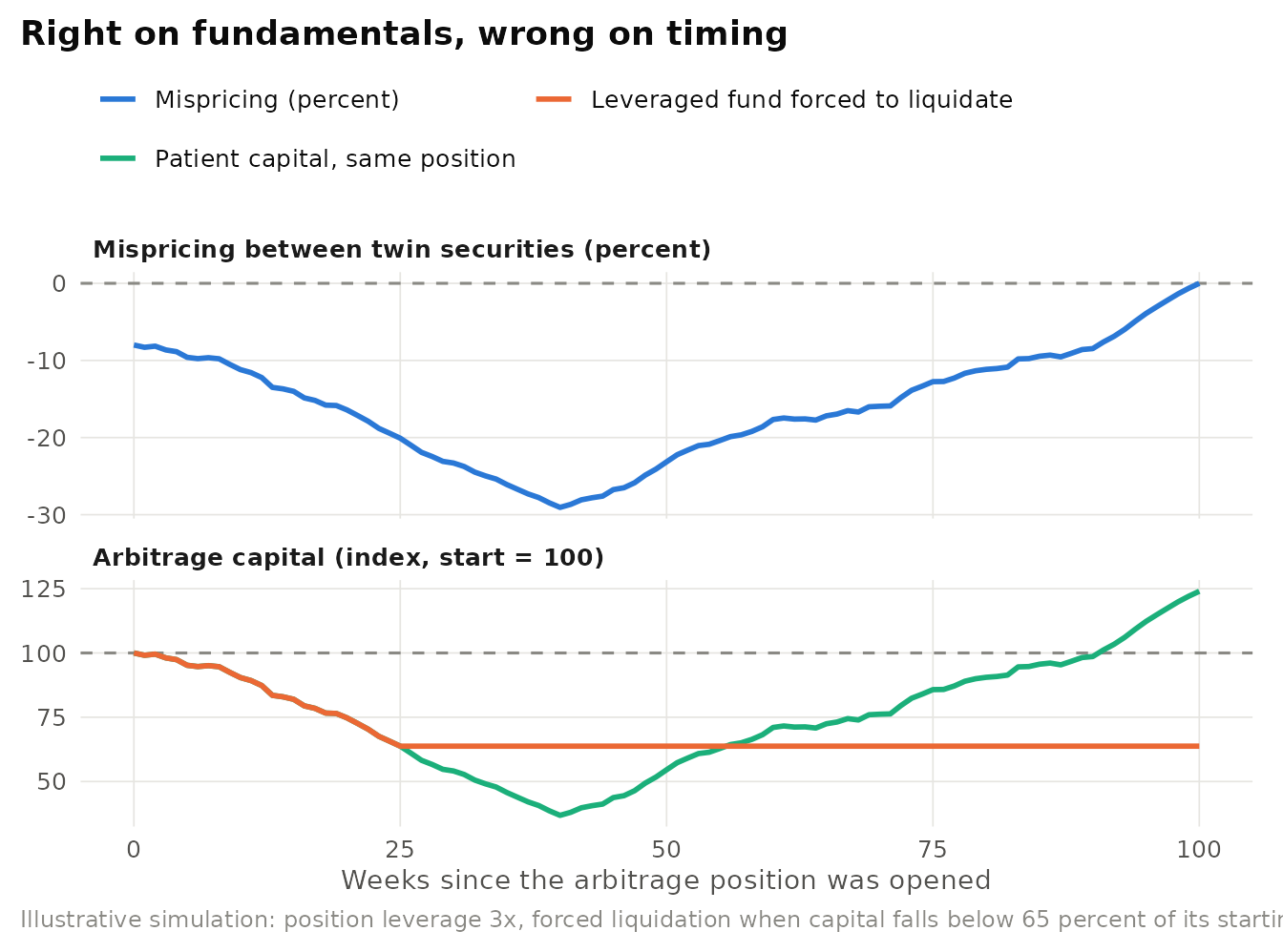
Figure 16.10: Illustrative performance-based arbitrage. Top: the mispricing between two claims on identical cash flows widens before it converges. Bottom: a leveraged arbitrage fund facing investor withdrawals is forced to liquidate near the worst point, while patient capital with the same position ends with a gain.

16.7.4 Evidence and extensions

The cleanest evidence comes from securities whose relative value is fixed by contract. Table 16.7 summarises four well-documented episodes.

Table 16.7: Episodes illustrating the limits to arbitrage.

Episode	What should have held	What happened	Limit to arbitrage
Royal Dutch and Shell (Froot & Dabora 1999)	Twin shares with a fixed split of cash flows should trade at a constant price ratio	The ratio deviated substantially from parity for years	Noise trader risk with no fixed convergence date
Palm and 3Com, 2000 (Lamont & Thaler 2003)	3Com, which still owned most of Palm, should be worth at least its Palm stake	The market implied a negative value for 3Com’s other businesses	Short-sale constraints on Palm shares
Long-Term Capital Management, 1998	Convergence trades should profit as spreads narrow	Spreads widened sharply after the Russian default and the fund lost most of its capital	Leverage, crowding, and forced liquidation
GameStop, January 2021 (SEC 2021)	Prices should reflect expected cash flows	The price rose roughly twentyfold in weeks and remained volatile	Short-selling risk, margin calls, and coordinated noise trading

The Royal Dutch and Shell case is particularly instructive. Under their 1907 alliance, cash flows were split 60 to 40, so Royal Dutch should have been worth 1.5 times Shell. Froot and Dabora (1999) showed that the ratio deviated from parity by large amounts for long periods. An arbitrageur betting on convergence faced no fundamental risk, only the risk that the deviation would widen, with no date by which it had to close.

Does limited arbitrage rescue or bury the EMH? Defenders of efficiency note that in each famous case the mispricing was eventually corrected and that it is hard to profit from these episodes after transaction costs. Behavioural economists reply that this is exactly the point: “no free lunch” does not imply “prices are right” (N. Barberis and Thaler 2003). If even riskless relative mispricing can persist, mispricing of whole markets, with no close substitute and no convergence date, can persist far longer. Still, limits to arbitrage explain why mispricing can persist, not which direction it takes. That requires a theory of investor beliefs.

16.7.5 Applications in business

Long-Term Capital Management, 1998. LTCM was founded in 1994 by John Meriwether, and its partners included Myron Scholes and Robert Merton, who shared the 1997 Nobel Memorial Prize for their work on option pricing. The fund specialised in convergence and relative-value trades, such as buying less liquid bonds and selling more liquid but otherwise similar bonds, betting that small price gaps would close. Because each gap was small, the strategy required very high leverage. After Russia defaulted on its domestic debt in August 1998, investors worldwide fled to the safest and most liquid securities. The spreads LTCM had bet would narrow widened instead, and because many other traders held similar positions, attempts to reduce risk pushed prices further against the fund. By September its capital had collapsed, and the Federal Reserve Bank of New York convened a group of major banks and securities firms that recapitalised the fund with about 3.6 billion dollars to avoid a disorderly liquidation (Lowenstein 2000, President’s Working Group on Financial Markets 1999). The episode is the textbook illustration of Shleifer and Vishny (1997), published a year earlier: arbitrage can fail when capital is leveraged, crowded, and impatient. Risk managers should stress-test for widening spreads and crowded positions.

16.7.6 Using the theory in research

Sample hypotheses.

• H1. Anomaly returns are larger among stocks with higher short-selling costs (lower institutional ownership, higher lending fees).
• H2. Hedge fund outflows following poor performance predict subsequent widening of mispricing in the stocks those funds hold.

Measures. Mispricing in contractually linked securities, idiosyncratic volatility as arbitrage risk, short interest and loan fees, fund flows, funding liquidity spreads.

Designs. Cross-sectional tests that interact anomaly signals with limits to arbitrage proxies, natural experiments from short-sale bans or changes in lending supply, case studies of contractually linked securities.

Using limits to arbitrage as a universal escape hatch. Almost any failure of a mispricing to correct can be attributed, after the fact, to some limit to arbitrage. To make the theory testable, specify in advance which limit (short-sale costs, idiosyncratic risk, capital constraints) should matter, measure it, and predict that mispricing will be greater where that limit is tighter.

16.8 Behavioral Finance

Core claim. Investor psychology produces systematic errors in beliefs and preferences, and because arbitrage is limited, these errors affect prices, trading, and corporate decisions.

Origins. Finance, economics, and psychology. Early contributions include Shefrin and Statman (1985) and De Long et al. (1990). N. Barberis and Thaler (2003) is the standard survey. Robert Shiller received the Nobel Memorial Prize in 2013 and Richard Thaler in 2017.

Level of analysis. Individual investor, manager, and market.

Key constructs. Overconfidence, disposition effect, extrapolation, limited attention, loss aversion (Section 24.4), mental accounting, investor sentiment, market timing.

Boundary conditions. Biases must be systematic (shared across many investors) to affect prices, and arbitrage must be costly. Effects are strongest for assets that are hard to value and hard to arbitrage.

Related theories. Limits to arbitrage, Prospect theory (Section 24.2), Disposition effect (Section 24.8), Heuristics and biases (Section 23.2), Mental accounting (Section 23.5), Conformity (Section 22.4), Social transmission (Section 26.3).

16.8.1 Origins and intellectual history

Behavioural finance grew from the confluence of two ideas. From psychology came evidence that people deviate systematically from expected utility and Bayesian updating, especially the work of Kahneman and Tversky on judgment under uncertainty and Prospect theory (Section 24.2) (Kahneman and Tversky 1979). From finance came the realisation, formalised by De Long et al. (1990) and Shleifer and Vishny (1997), that rational arbitrage need not eliminate the price effects of irrational traders. N. Barberis and Thaler (2003) describe the field as resting on these two building blocks: limits to arbitrage, which explain why mispricing can survive, and psychology, which explains what form it takes.

16.8.2 Core logic and propositions

• P1 (Overconfidence and trading). Investors who overestimate the precision of their information trade too much and earn lower net returns.
• P2 (Disposition effect). Investors realise gains more readily than losses, a pattern consistent with prospect theory (Chapter 24) and mental accounting.
• P3 (Sentiment). Waves of investor optimism and pessimism move the prices of hard-to-value, hard-to-arbitrage stocks more than others, and high sentiment predicts low subsequent returns for those stocks.
• P4 (Managerial response). Managers respond to mispricing by issuing equity when it is overvalued and buying back shares when it is undervalued, and their own biases shape investment.

16.8.3 Mechanism

Figure 16.11 shows how the building blocks combine. Psychological biases generate correlated demand. Limits to arbitrage allow that demand to move prices. Mispricing then feeds back into corporate decisions through equity issuance, repurchases, and investment.

Figure 16.11: Mechanism of behavioural finance. Systematic biases create correlated noise trading. When arbitrage is limited, prices deviate from fundamentals, which affects returns and induces managers to time security issues and repurchases.

16.8.4 Evidence and extensions

Overconfidence. Using records from a large discount brokerage, Barber and Odean (2000) found that the households that traded most earned substantially lower net returns than the market, largely because of trading costs. Barber and Odean (2001) then used gender as a proxy for overconfidence, motivated by evidence that men are more overconfident than women in domains such as finance. Men traded about 45 percent more than women, and trading reduced men’s net returns by more than it reduced women’s.

Disposition effect. Shefrin and Statman (1985) argued that investors are predisposed to sell winners too early and ride losers too long. Odean (1998) confirmed the pattern in brokerage data: investors realised a higher proportion of their gains than of their losses, and the winners they sold went on to outperform the losers they kept. See the Disposition effect (Section 24.8) for a full treatment.

Investor sentiment. M. Baker and Wurgler (2006) built a composite sentiment index from proxies such as the closed-end fund discount, share turnover, the number and first-day returns of IPOs, the equity share of new issues, and the dividend premium. When sentiment was high, subsequent returns were relatively low for small, young, highly volatile, unprofitable, non-dividend-paying, extreme growth, and distressed stocks, and when sentiment was low the pattern reversed. These are exactly the stocks that are hardest to value and hardest to arbitrage, as P3 predicts. Figure 16.12 sketches the pattern.

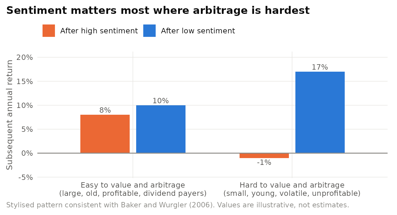
Figure 16.12: Stylised pattern of sentiment and subsequent returns. Hard-to-value stocks earn low returns after periods of high sentiment and high returns after periods of low sentiment, while easy-to-value stocks are little affected. Not empirical data.

Corporate decisions. Rational managers can exploit mispricing by timing equity issues (M. Baker and Wurgler 2002), and managers have biases too: overconfident CEOs overinvest (Malmendier and Tate 2005) and acquirers may overpay because of hubris (Roll 1986). Table 16.8 organises the main findings.

Table 16.8: Behavioural biases in finance: roots, consequences, and evidence.

Bias	Psychological root	Market or firm consequence	Key evidence	Practical implication
Overconfidence	Miscalibrated precision of private information	Excessive trading, lower net returns	Barber & Odean (2000, 2001)	Default to low-turnover strategies, cost disclosure
Disposition effect	Prospect theory, mental accounting, regret	Selling winners and holding losers, drift after news	Shefrin & Statman (1985), Odean (1998)	Rule-based selling, tax-loss harvesting
Extrapolation	Representativeness, recency	Overpricing of glamour stocks, reversals	Barberis & Thaler (2003)	Skepticism toward trend-based forecasts
Limited attention	Finite cognitive resources	Underreaction to news, earnings drift	Bernard & Thomas (1989)	Timing and salience of disclosures
Sentiment	Correlated mood and beliefs	Mispricing of hard-to-value stocks	Baker & Wurgler (2006)	Equity issuance when sentiment is high
Managerial overconfidence	Better-than-average beliefs	Overinvestment and costly acquisitions	Malmendier & Tate (2005), Roll (1986)	Independent boards, investment hurdles

Anomalies or a theory? The strongest criticism of behavioural finance comes from Fama (1998), who argued that the literature had produced a list of anomalies rather than a theory: some studies find underreaction, others overreaction, and many anomalies are sensitive to methodology. Behavioural researchers have responded with models that derive both patterns from a few psychological assumptions, with out-of-sample tests such as those of sentiment indices (M. Baker and Wurgler 2006), and with individual trading data in which biases can be observed directly (Odean 1998, Barber and Odean 2001). Biases observed in trading records have generally proved sturdier than return anomalies, many of which have shrunk since publication (McLean and Pontiff 2016).

16.8.5 Applications in business

GameStop, January 2021. In late 2020 GameStop, a struggling video-game retailer, was one of the most heavily shorted stocks in the US market, with reported short interest exceeding the number of shares available for trading. Retail investors, many coordinating on the Reddit forum r/wallstreetbets and trading through commission-free apps, began buying the shares and call options. The price rose from under 20 dollars at the start of January 2021 to a closing high above 300 dollars on 27 January. Several hedge funds with short positions suffered large losses, and one, Melvin Capital, received a multibillion-dollar capital infusion from other investment firms. On 28 January several brokers restricted purchases of GameStop and other “meme stocks”, citing sharply higher collateral requirements at their clearinghouse. The SEC staff report on the episode found that short covering accounted for only a small part of the buying and that the rise was driven mainly by investors who were not covering short positions (U.S. Securities and Exchange Commission 2021).

The episode combines the chapter’s theories. Social contagion and sentiment, see Social transmission (Section 26.3) and Conformity (Section 22.4), produced correlated noise trading. Short sellers faced unlimited potential losses and margin calls, so betting against the rally was extremely risky even for investors convinced that the price exceeded fundamental value, as De Long et al. (1990) and Shleifer and Vishny (1997) predict. GameStop then sold new shares at the elevated price later in 2021, the market timing of M. Baker and Wurgler (2002).

16.8.6 Using the theory in research

Sample hypotheses.

• H1. Retail investors who receive more push notifications trade more frequently and earn lower risk-adjusted net returns, an effect moderated by financial literacy.
• H2. Firms issue more equity and conduct fewer repurchases when sentiment for their industry is high, controlling for investment opportunities.

Measures. Turnover, realised gains and losses (PGR and PLR), sentiment indices, social media attention, short interest, retail order flow, issuance and repurchase activity.

Designs. Account-level brokerage data, field experiments on information presentation, natural experiments from app feature rollouts, panel regressions of issuance on sentiment, laboratory asset markets.

Naming a bias instead of testing it. It is easy to label any pattern in returns with a bias after the fact. A credible behavioural finance study derives a prediction from a specific psychological mechanism, shows that the mechanism operates in the population studied, and rules out risk-based and institutional explanations, ideally with a test where the behavioural and rational accounts predict different outcomes.

16.9 Chapter Summary

• Portfolio theory: risk is a property of portfolios. Diversification removes idiosyncratic risk (Markowitz 1952, Tobin 1958).
• The CAPM prices only systematic risk through beta (Sharpe 1964, Lintner 1965). Its empirical failures led to multifactor models (Fama and French 1992, 1993).
• The efficient market hypothesis holds that prices reflect available information (Fama 1970). Index funds rest on its most robust implication (Sharpe 1991), while excess volatility shows that prices need not equal fundamental value (Shiller 1981).
• The Modigliani-Miller theorems make financing irrelevant in perfect markets (Modigliani and Miller 1958), turning every friction, starting with taxes (Modigliani and Miller 1963), into a candidate theory of capital structure.
• The trade-off and pecking order theories explain leverage through tax shields and distress costs, and through information asymmetry, respectively. Neither fully fits the data (Myers 1984, Shyam-Sunder and Myers 1999, Frank and Goyal 2003).
• Free cash flow theory explains why debt, payouts, and takeovers can create value in mature, cash-rich firms (Jensen 1986).
• Limits to arbitrage explain why mispricing persists: arbitrage is risky and capital is impatient (De Long et al. 1990, Shleifer and Vishny 1997).
• Behavioral finance combines limits to arbitrage with investor psychology to explain trading, anomalies, and corporate financing choices (N. Barberis and Thaler 2003).

Table 16.9 presents the comparison of the chapter’s theories.

Table 16.9: Comparison of the chapter’s theories.

Theory	Core mechanism	Signature prediction	Main challenge	Typical business use
Portfolio theory	Covariance and diversification	Efficient portfolios dominate concentrated ones	Estimation error in inputs	Asset allocation, retirement plans
CAPM	Only systematic risk is priced	Expected returns linear in beta	Flat SML, size, value, momentum	Cost of capital, performance evaluation
Efficient market hypothesis	Competition among informed traders	No predictable abnormal returns	Anomalies, excess volatility	Index funds, event studies
Modigliani-Miller	Arbitrage and homemade leverage	Financing irrelevant in perfect markets	Assumptions rarely hold	Benchmark for financing decisions
Trade-off and pecking order	Taxes versus distress, information asymmetry	Target leverage or financing hierarchy	Persistence, market timing	Leverage and issuance policy
Free cash flow theory	Agency costs of surplus cash	Debt and payouts discipline managers	Precautionary cash holdings	Payout policy, buyouts
Limits to arbitrage	Risky, capital-constrained arbitrage	Mispricing persists where arbitrage is hard	Ex post flexibility	Risk management, hedge fund design
Behavioral finance	Investor biases plus limits to arbitrage	Sentiment and bias-driven mispricing	Many anomalies, few unified models	Product design, market timing

16.10 Discussion Questions

1. Many founders and executives hold most of their wealth in a single firm. Using agency theory and portfolio theory, explain when such concentration is efficient for the firm even if it is costly for the individual.
2. The CAPM fails many empirical tests yet remains the most common method for estimating the cost of equity. Is this a failure of practice or a defensible choice?
3. Design an event study of a sustainability announcement. Which form of market efficiency must hold for your estimate to be meaningful?
4. A CFO argues that because debt is cheaper than equity, more leverage lowers the cost of capital. Evaluate the argument with the Modigliani-Miller propositions and the trade-off theory.
5. Large technology firms hold very large cash balances. Develop competing hypotheses from free cash flow and pecking order theory, and describe data that could distinguish them.
6. Using the GameStop episode, explain why short sellers who believed the stock was overvalued might rationally have closed their positions. What does this imply for price efficiency during episodes of extreme sentiment?

16.11 Further Reading

• Markowitz (1952): the short paper that founded modern portfolio theory and remains a model of clear argument.
• Fama and French (2004): an accessible review of the CAPM’s logic, its empirical record, and why its failures matter for practice.
• Fama (1970): the classic synthesis of market efficiency, with the three forms and the joint hypothesis problem.
• Myers (2001): a lucid survey of capital structure theories from Modigliani-Miller through the trade-off and pecking order debates.
• Jensen (1986): a compact statement of free cash flow theory that shaped two decades of research on payouts and takeovers.
• Shleifer and Vishny (1997): the paper that explains why arbitrage fails when it is most needed, vindicated by the LTCM crisis a year later.
• N. Barberis and Thaler (2003): the standard survey of behavioural finance, organised around limits to arbitrage and investor psychology.
• French (2008): a careful accounting of what investors spend trying to beat the market, essential background for the index fund debate.