Textual analysis has emerged as one of the most productive research frontiers in empirical finance over the past two decades. The insight that unstructured text, such as corporate filings, earnings calls, analyst reports, and news articles, contains economically meaningful information beyond what is captured in structured numerical data has reshaped how researchers and practitioners understand financial markets. This chapter introduces the full pipeline of textual analysis methods as applied to Vietnamese listed firms, progressing from classical bag-of-words approaches through modern transformer-based language models.
The Vietnamese equity market presents unique opportunities and challenges for textual analysis. As of 2024, the Ho Chi Minh Stock Exchange (HOSE) and the Hanoi Stock Exchange (HNX) together list over 1,600 securities with a combined market capitalization exceeding VND 6,000 trillion (approximately USD 240 billion). Corporate disclosures are filed in Vietnamese, a tonal language with compound-word morphology that demands specialized natural language processing (NLP) tools.
We build on the seminal contributions of Loughran and McDonald (2011) in domain-specific sentiment lexicons, Hoberg and Phillips (2016) in text-based industry classification, and the modern deep learning revolution initiated by Devlin et al. (2019). This chapter covers the following topics:
Constructing the universe of HOSE/HNX listed firms and retrieving their business descriptions and annual report text.
Vietnamese-specific text preprocessing, including word segmentation using VnCoreNLP and underthesea.
Classical document representation via bag-of-words, TF-IDF, and LDA topic models.
Financial sentiment analysis using both dictionary-based and machine learning approaches adapted for Vietnamese.
Text-based firm similarity and peer identification using cosine similarity.
Modern deep learning approaches including Word2Vec, Doc2Vec, PhoBERT embeddings, and sentence transformers.
Large language model (LLM) applications, including zero-shot classification, named entity recognition, and information extraction using Vietnamese-capable models.
Empirical applications linking textual measures to stock returns, volatility, and corporate events.
46.1 Why Textual Analysis for Vietnamese Finance?
The Vietnamese financial market has several characteristics that make textual analysis particularly valuable. First, analyst coverage is sparse (fewer than 30% of listed firms receive regular coverage from sell-side analysts), making alternative information sources critical. Second, the regulatory environment is evolving rapidly, with the State Securities Commission (SSC) continuously updating disclosure requirements, creating rich variation in information environments across firms and time. Third, the market is dominated by retail investors (accounting for roughly 80% of trading volume), who may process textual information differently than institutional investors, creating potential mispricings that text-based strategies could exploit.
From a methodological standpoint, Vietnamese poses interesting NLP challenges. Unlike English, Vietnamese is an isolating language where word boundaries are not always delimited by spaces. A single Vietnamese “word” may consist of multiple syllables separated by spaces (e.g., “công ty” for “company,” “thị trường” for “market”). This requires a word segmentation step before standard NLP pipelines can be applied.1
47 Literature Review
47.1 Textual Analysis in Finance
The application of textual analysis to financial data has a rich history. Tetlock (2007) demonstrated that the pessimism content of a Wall Street Journal column predicts aggregate market activity, providing early evidence that textual content moves prices. Loughran and McDonald (2011) showed that the widely-used Harvard General Inquirer sentiment dictionary produces misleading results when applied to financial text because words like “liability,” “tax,” and “capital” are classified as negative in general English but carry neutral or even positive connotations in finance. Their domain-specific word lists have become the standard for financial sentiment analysis.2
Hoberg and Phillips (2010) and Hoberg and Phillips (2016) pioneered the use of product descriptions from 10-K filings to construct text-based industry classifications (TNIC), demonstrating that these dynamic, firm-specific industry definitions outperform static SIC and NAICS codes in explaining firm behavior, including profitability, stock returns, and M&A activity. Subsequent work by Hoberg and Phillips (2018) extended this to assess competitive threats and product-market fluidity.
More recent work has leveraged advances in deep learning. Huang, Wang, and Yang (2023) apply BERT-based models to earnings call transcripts and show that contextual embeddings capture information about future earnings that traditional bag-of-words measures miss. Jha et al. (2024) use GPT-based models for zero-shot financial text classification and demonstrate that LLMs can match or exceed purpose-built classifiers on standard benchmarks. Earnings calls are also read by regulators: Lerman, Steffen, and Zhang (2026) show that the SEC cites voluntary call disclosures in comment letters, mostly to show that the mandatory filing says too little, and that firms then change their filings (Section 55.6).
Text can also measure the uncertainty investors face, not only its tone. Wei and Zhang (2026) extract a narrative-based ambiguity measure from economic news articles, distinct from survey- and return-based ambiguity proxies, and show that it predicts aggregate stock market returns both in and out of sample. Investors are on average ambiguity averse, but ambiguity tolerance emerges when the probability of loss is high, and aligning industry-specific narrative ambiguity (chiefly from consumption-, energy-, and technology-related news) yields a stronger market predictor. The predictability extends to international markets and other asset classes, which makes the approach a natural candidate for Vietnamese financial news.
47.2 NLP for Vietnamese Language
Vietnamese NLP has advanced significantly with the development of VnCoreNLP (Vu et al. 2018), a Java-based toolkit providing word segmentation, POS tagging, named entity recognition, and dependency parsing. The underthesea library offers a Python-native alternative. Most critically for financial applications, PhoBERT (Nguyen and Nguyen 2020) provides Vietnamese-specific BERT pre-training on a 20GB corpus, achieving state-of-the-art results on multiple Vietnamese NLP tasks.
Table 47.1: Key Literature on Textual Analysis in Finance
Table 48.1: Universe of Vietnamese Listed Firms by Exchange (as of December 2024)
Exchange
N Firms
Avg Mkt Cap (VND bn)
Median Mkt Cap (VND bn)
Total Mkt Cap (VND tn)
HOSE
403
12,847
3,215
5,177
HNX
334
2,156
687
720
UPCoM
868
1,043
298
905
Total
1,605
4,239
712
6,802
48.2 Retrieving Business Descriptions
Business descriptions for all listed firms can be in both Vietnamese and English. We retrieve both versions for our analysis. The Vietnamese text will serve as the primary corpus, while English descriptions provide a useful cross-validation.
Retrieve business descriptions.
# Get business descriptions (Vietnamese and English)bus_desc = dc.get_business_descriptions( tickers=universe.ticker.tolist(), fields=['ticker', 'bus_desc_vi', 'bus_desc_en','main_business', 'products_services','year_established', 'num_employees' ])# Merge with universecorpus_df = universe.merge(bus_desc, on='ticker', how='inner')# Summary statistics on text lengthcorpus_df['desc_len_vi'] = corpus_df.bus_desc_vi.str.len()corpus_df['desc_len_en'] = corpus_df.bus_desc_en.str.len()corpus_df['word_count_vi'] = corpus_df.bus_desc_vi.str.split().str.len()print(corpus_df[['desc_len_vi', 'desc_len_en', 'word_count_vi']] .describe().round(0))
Table 48.2: Descriptive Statistics of Business Description Text
Statistic
Mean
Median
Std Dev
Min
Max
Characters (VN)
2,847
2,156
1,923
87
18,432
Characters (EN)
3,412
2,689
2,245
102
22,156
Words (VN)
487
372
318
15
3,216
48.3 Retrieving Annual Report Text
Beyond business descriptions, annual or quarterly reports provide richer and more time-varying textual data. We extract the Management Discussion and Analysis (MD&A) sections, which are most informative for financial analysis (Li et al. 2010; Bonsall IV et al. 2017). The MD&A section, known in Vietnamese annual reports as “Báo cáo của Ban Giám đốc” or “Báo cáo của Hội đồng quản trị,” discusses business performance, outlook, and risk factors.
Retrieve annual report MD&A sections
# Get annual report MD&A sections (2015-2024)annual_text = dc.get_annual_report_text( tickers=universe.ticker.tolist(), years=range(2015, 2025), sections=['mda', 'risk_factors', 'business_overview'], language='vi')# Panel structure: ticker x year x sectionprint(f'Total firm-year-section observations: {len(annual_text)}')print(f'Unique firms: {annual_text.ticker.nunique()}')print(f'Year range: {annual_text.year.min()}-{annual_text.year.max()}')# Calculate text changes year-over-yearannual_text = annual_text.sort_values(['ticker', 'year'])annual_text['text_len'] = annual_text.text.str.len()annual_text['text_change_pct'] = ( annual_text.groupby('ticker')['text_len'] .pct_change() *100)
49 Text Preprocessing for Vietnamese
49.1 Vietnamese Word Segmentation
The most critical preprocessing step for Vietnamese text is word segmentation (phân đoạn từ). Unlike English where spaces reliably separate words, Vietnamese uses spaces between syllables, not between words. For example, the phrase “công ty cổ phần bất động sản” (real estate joint stock company) contains five syllables separated by spaces but consists of only two compound words: “công_ty cổ_phần” (joint stock company) and “bất_động_sản” (real estate). Failing to perform word segmentation leads to severe vocabulary fragmentation and loss of semantic meaning.
Table 49.1: Vietnamese Word Segmentation Example
Stage
Text
Interpretation
Raw
công ty cổ phần thương mại dịch vụ
7 syllables, ambiguous boundaries
Segmented
công_ty cổ_phần thương_mại dịch_vụ
4 words: company | joint-stock | commerce | services
Vietnamese word segmentation using underthesea
from underthesea import word_tokenizedef segment_vietnamese(text: str) ->str:"""Segment Vietnamese text into words using underthesea."""if pd.isna(text) or text.strip() =='':return''# underthesea word_tokenize joins compound words with _ segmented = word_tokenize(text, format='text')return segmented# Alternative: VnCoreNLP (Java-based, higher accuracy)# from vncorenlp import VnCoreNLP# vnlp = VnCoreNLP('VnCoreNLP-1.2.jar', annotators='wseg')# segmented = vnlp.tokenize(text)# Apply segmentation to corpuscorpus_df['bus_desc_segmented'] = ( corpus_df.bus_desc_vi.apply(segment_vietnamese))# Examplesample = corpus_df.iloc[0]print('Raw:', sample.bus_desc_vi[:200])print('Segmented:', sample.bus_desc_segmented[:200])
49.2 Full Text Cleaning Pipeline
After word segmentation, we apply a cleaning pipeline. The pipeline handles Vietnamese-specific challenges including: diacritical mark normalization (e.g., hoà vs hòa), removal of HTML artifacts from scraped text, Vietnamese stopword removal, and lemmatization (which for Vietnamese primarily involves handling reduplicative words and synonym normalization).
Full Vietnamese text cleaning pipeline
# Vietnamese stopwords (domain-adapted)VIETNAMESE_STOPWORDS = {'có', 'là', 'và', 'của', 'cho', 'được', 'trong','các', 'những', 'với', 'từ', 'khi', 'hoặc','đã', 'sẽ', 'đang', 'để', 'này', 'đó','như', 'theo', 'về', 'bằng', 'tại', 'trên','cũng', 'rất', 'nhiều', 'ít', 'một', 'hai',# Financial domain stopwords'năm', 'quý', 'tháng', 'ngày', 'kỳ','việt_nam', 'tổng', 'giá_trị', 'triệu', 'tỷ',}def clean_vietnamese_text( text: str, segment: bool=True, remove_stops: bool=True, lowercase: bool=True, min_word_len: int=2) ->str:""" Full Vietnamese text cleaning pipeline. Parameters ---------- text : str Raw Vietnamese text. segment : bool Whether to perform word segmentation. remove_stops : bool Whether to remove Vietnamese stopwords. lowercase : bool Whether to convert to lowercase. min_word_len : int Minimum word length to keep. Returns ------- str Cleaned text. """if pd.isna(text) or text.strip() =='':return''# 1. Unicode normalization (NFC form for Vietnamese) text = unicodedata.normalize('NFC', text)# 2. Remove HTML tags and special characters text = re.sub(r'<[^>]+>', ' ', text) text = re.sub(r'[\d]+', ' ', text) # Remove numbers text = re.sub(r'[^\w\s\u00C0-\u024F]', ' ', text) # Keep VN chars# 3. Lowercaseif lowercase: text = text.lower()# 4. Word segmentationif segment: text = word_tokenize(text, format='text')# 5. Tokenize and filter tokens = text.split()if remove_stops: tokens = [t for t in tokensif t notin VIETNAMESE_STOPWORDSandlen(t) >= min_word_len]return' '.join(tokens)# Apply to corpuscorpus_df['text_clean'] = ( corpus_df.bus_desc_vi .apply(lambda x: clean_vietnamese_text(x)))# Verify cleaning qualityprint('Sample cleaned text:')print(corpus_df.iloc[0].text_clean[:300])
49.3 English Text Cleaning
For firms that also provide English business descriptions, we apply a standard English NLP pipeline using spaCy and NLTK. This parallel processing enables cross-lingual validation of our textual measures.
English text cleaning pipeline
import spacyfrom nltk.corpus import stopwordsimport gensimnlp = spacy.load('en_core_web_sm', disable=['parser', 'ner'])stop_words =set(stopwords.words('english'))def clean_english_text(text: str) ->str:"""Clean English text with lemmatization."""if pd.isna(text) or text.strip() =='':return'' text = text.lower().strip() text = re.sub(r'[^a-zA-Z\s]', ' ', text) doc = nlp(text) tokens = [token.lemma_ for token in docif token.lemma_ notin stop_wordsandlen(token.lemma_) >2andnot token.is_punct]return' '.join(tokens)# Apply to English descriptionscorpus_df['text_clean_en'] = ( corpus_df.bus_desc_en .apply(lambda x: clean_english_text(x)))
50 Document Representation: Bag-of-Words and TF-IDF
50.1 Bag-of-Words Representation
The bag-of-words (BoW) model represents each document as a vector of word frequencies, discarding word order. Despite its simplicity, BoW remains a workhorse in financial textual analysis. Formally, given a vocabulary \(V = \{w_1, w_2, \ldots, w_{|V|}\}\), document \(d\) is represented as a vector \(\mathbf{x}_d\) where each element \(x_{d,j}\) counts the frequency of word \(w_j\) in document \(d\):
where \(\text{tf}(w, d)\) is the term frequency of word \(w\) in document \(d\).
Bag-of-Words vectorization
from sklearn.feature_extraction.text import ( CountVectorizer, TfidfVectorizer)# Vietnamese corpustext_corpus = corpus_df.text_clean.tolist()# BoW vectorizationbow_vectorizer = CountVectorizer( max_features=10000, min_df=5, # Appear in at least 5 documents max_df=0.95, # Exclude terms in >95% of docs ngram_range=(1, 2) # Unigrams and bigrams)bow_matrix = bow_vectorizer.fit_transform(text_corpus)print(f'Vocabulary size: {len(bow_vectorizer.vocabulary_)}')print(f'Document-term matrix shape: {bow_matrix.shape}')print(f'Sparsity: {1- bow_matrix.nnz / np.prod(bow_matrix.shape):.4f}')# Top 20 most frequent termsword_freq = pd.DataFrame({'word': bow_vectorizer.get_feature_names_out(),'freq': bow_matrix.sum(axis=0).A1}).sort_values('freq', ascending=False)print('\nTop 20 most frequent terms:')print(word_freq.head(20).to_string(index=False))
Plot word frequency distribution
fig, ax = plt.subplots(figsize=(12, 6))top20 = word_freq.head(20)ax.barh(range(len(top20)), top20.freq.values, color='#2C5282')ax.set_yticks(range(len(top20)))ax.set_yticklabels(top20.word.values)ax.invert_yaxis()ax.set_xlabel('Frequency')ax.set_title('Top 20 Most Frequent Terms in Vietnamese Business Descriptions')plt.tight_layout()plt.show()
Figure 50.1
Table 50.1: Top 20 Most Frequent Terms in Vietnamese Business Descriptions
#
Term (VN)
Freq
#
Term (VN)
Freq
#
Term (VN)
Freq
1
sản_xuất
4,287
8
công_nghệ
1,956
15
xuất_khẩu
1,123
2
kinh_doanh
3,891
9
tài_chính
1,845
16
bất_động_sản
1,087
3
dịch_vụ
3,654
10
ngân_hàng
1,734
17
năng_lượng
1,045
4
công_ty
3,412
11
đầu_tư
1,623
18
bảo_hiểm
987
5
thương_mại
2,876
12
xây_dựng
1,534
19
du_lịch
923
6
cổ_phần
2,543
13
vận_tải
1,345
20
viễn_thông
876
7
chứng_khoán
2,134
14
thực_phẩm
1,234
50.2 TF-IDF Weighting
Term Frequency-Inverse Document Frequency (TF-IDF) addresses a key limitation of raw term counts by downweighting terms that appear in many documents (and thus carry less discriminative information). The TF-IDF weight of term \(w\) in document \(d\) within corpus \(D\) is:
where \(|D|\) is the total number of documents and \(\text{df}(w, D)\) is the number of documents containing term \(w\). This weighting scheme ensures that industry-specific terminology (e.g., “khai_khoáng” for mining, “dược_phẩm” for pharmaceuticals) receives higher weight than ubiquitous corporate jargon.
TF-IDF vectorization with per-industry analysis
tfidf_vectorizer = TfidfVectorizer( max_features=10000, min_df=5, max_df=0.95, ngram_range=(1, 2), sublinear_tf=True# Use 1 + log(tf) instead of raw tf)tfidf_matrix = tfidf_vectorizer.fit_transform(text_corpus)# Per-industry top TF-IDF termsfor industry in ['Ngân hàng', 'Bất động sản','Công nghệ thông tin']: mask = corpus_df.icb_sector == industryif mask.sum() ==0:continue mean_tfidf = tfidf_matrix[mask.values].mean(axis=0).A1 top_idx = mean_tfidf.argsort()[-10:][::-1] terms = tfidf_vectorizer.get_feature_names_out()print(f'\n{industry}:')for idx in top_idx:print(f' {terms[idx]}: {mean_tfidf[idx]:.4f}')
Visualize industry-distinctive terms
# Build industry x term TF-IDF matrix for top sectorstop_sectors = corpus_df.icb_sector.value_counts().head(8).index.tolist()terms = tfidf_vectorizer.get_feature_names_out()sector_tfidf = {}for sector in top_sectors: mask = corpus_df.icb_sector == sectorif mask.sum() ==0:continue mean_tfidf = tfidf_matrix[mask.values].mean(axis=0).A1 top_idx = mean_tfidf.argsort()[-5:][::-1]for idx in top_idx:if terms[idx] notin sector_tfidf: sector_tfidf[terms[idx]] = {} sector_tfidf[terms[idx]][sector] = mean_tfidf[idx]heatmap_df = pd.DataFrame(sector_tfidf).T.fillna(0)fig, ax = plt.subplots(figsize=(14, 10))sns.heatmap(heatmap_df, annot=True, fmt='.3f', cmap='Blues', linewidths=0.5, ax=ax)ax.set_title('TF-IDF Heatmap: Industry-Distinctive Terms')ax.set_xlabel('ICB Sector')ax.set_ylabel('Term')plt.tight_layout()plt.show()
Figure 50.2
51 Topic Modeling
51.1 Latent Dirichlet Allocation (LDA)
Latent Dirichlet Allocation (Blei, Ng, and Jordan 2003) is a generative probabilistic model that discovers latent topics in a corpus. Each document is modeled as a mixture of topics, and each topic is a distribution over words. LDA has been widely applied in finance to identify thematic content in 10-K filings (Dyer, Lang, and Stice-Lawrence 2017), earnings calls (Huang et al. 2018), and news articles (Bybee, Kelly, and Su 2023).
The generative process assumes:
For each topic \(k\), draw a word distribution \(\boldsymbol{\phi}_k \sim \text{Dir}(\beta)\).
For each document \(d\), draw a topic distribution \(\boldsymbol{\theta}_d \sim \text{Dir}(\alpha)\).
For each word position \(i\) in document \(d\), draw a topic \(z_{d,i} \sim \text{Multinomial}(\boldsymbol{\theta}_d)\) and then draw the word \(w_{d,i} \sim \text{Multinomial}(\boldsymbol{\phi}_{z_{d,i}})\).
LDA topic modeling with grid search over K
from sklearn.decomposition import LatentDirichletAllocation# Grid search over number of topicsn_topics_range = [10, 15, 20, 25, 30]perplexity_scores = []for n_topics in n_topics_range: lda = LatentDirichletAllocation( n_components=n_topics, max_iter=50, learning_method='online', random_state=42, n_jobs=-1 ) lda.fit(bow_matrix) perplexity = lda.perplexity(bow_matrix) perplexity_scores.append({'n_topics': n_topics,'perplexity': perplexity,'log_likelihood': lda.score(bow_matrix) })print(f'K={n_topics}: perplexity={perplexity:.2f}')# Select optimal K (e.g., K=20)K_OPTIMAL =20lda_model = LatentDirichletAllocation( n_components=K_OPTIMAL, max_iter=100, learning_method='online', random_state=42, n_jobs=-1)lda_model.fit(bow_matrix)# Extract topic-word distributionsfeature_names = bow_vectorizer.get_feature_names_out()for topic_idx, topic inenumerate(lda_model.components_): top_words = [feature_names[i]for i in topic.argsort()[:-11:-1]]print(f'Topic {topic_idx}: {" | ".join(top_words)}')
Plot perplexity scores for topic model selection
perp_df = pd.DataFrame(perplexity_scores)fig, ax = plt.subplots(figsize=(8, 5))ax.plot(perp_df.n_topics, perp_df.perplexity, 'o-', color='#2C5282', linewidth=2, markersize=8)ax.axvline(x=K_OPTIMAL, color='red', linestyle='--', alpha=0.7, label=f'Selected K={K_OPTIMAL}')ax.set_xlabel('Number of Topics (K)')ax.set_ylabel('Perplexity (lower is better)')ax.set_title('LDA Model Selection')ax.legend()plt.tight_layout()plt.show()
Figure 51.1
Table 51.1: Selected LDA Topics from Vietnamese Business Descriptions (K=20)
BERTopic (Grootendorst 2022) represents a significant advance over LDA by leveraging pre-trained language model embeddings, dimensionality reduction via UMAP, and hierarchical density-based clustering (HDBSCAN) to discover topics. Unlike LDA, BERTopic captures semantic similarity rather than relying solely on word co-occurrence, producing more coherent topics, especially for specialized domains.
BERTopic with PhoBERT embeddings
from bertopic import BERTopicfrom sentence_transformers import SentenceTransformerfrom umap import UMAPfrom hdbscan import HDBSCAN# Use PhoBERT-based sentence transformer for Vietnameseembedding_model = SentenceTransformer('bkai-foundation-models/vietnamese-bi-encoder')# Custom UMAP and HDBSCAN for better controlumap_model = UMAP( n_neighbors=15, n_components=5, min_dist=0.0, metric='cosine', random_state=42)hdbscan_model = HDBSCAN( min_cluster_size=10, min_samples=5, metric='euclidean', prediction_data=True)# Fit BERTopictopic_model = BERTopic( embedding_model=embedding_model, umap_model=umap_model, hdbscan_model=hdbscan_model, language='multilingual', calculate_probabilities=True, verbose=True)# Vietnamese text (use segmented text for better results)docs = corpus_df.bus_desc_segmented.tolist()topics, probs = topic_model.fit_transform(docs)# Inspect topicstopic_info = topic_model.get_topic_info()print(topic_info.head(20))
We construct a Vietnamese financial sentiment lexicon following the methodology of Loughran and McDonald (2011). Rather than directly translating the English LM dictionary (which would miss Vietnamese-specific financial expressions), we adopt a hybrid approach: (1) translate the core LM word lists using professional financial translators, (2) manually curate additions from Vietnamese financial regulation, accounting standards (VAS), and market commentary, and (3) validate the resulting dictionary against human-annotated Vietnamese financial text.
# Load Vietnamese financial sentiment lexicon# sentiment_dict = dc.get_sentiment_lexicon(version='vn_financial_v2')# Alternatively, construct from LM + manual curationnegative_words =set(pd.read_csv('lexicons/vn_negative.txt', header=None)[0])positive_words =set(pd.read_csv('lexicons/vn_positive.txt', header=None)[0])uncertain_words =set(pd.read_csv('lexicons/vn_uncertain.txt', header=None)[0])def compute_sentiment_scores(text: str) ->dict:""" Compute Loughran-McDonald style sentiment scores. Returns proportions (word count / total words). """ tokens = text.split() n =len(tokens)if n ==0:return {'neg_pct': 0, 'pos_pct': 0,'unc_pct': 0, 'net_tone': 0} neg =sum(1for t in tokens if t in negative_words) pos =sum(1for t in tokens if t in positive_words) unc =sum(1for t in tokens if t in uncertain_words)return {'neg_pct': neg / n,'pos_pct': pos / n,'unc_pct': unc / n,'net_tone': (pos - neg) / n }# Apply to annual report MD&A textsentiment_scores = annual_text.text_clean.apply(lambda x: pd.Series(compute_sentiment_scores(x)))annual_text = pd.concat([annual_text, sentiment_scores], axis=1)
Plot sentiment distribution
fig, axes = plt.subplots(1, 3, figsize=(15, 5))axes[0].hist(annual_text.neg_pct, bins=50, color='#E53E3E', alpha=0.7, edgecolor='white')axes[0].set_title('Negative Word Proportion')axes[0].set_xlabel('Proportion')axes[1].hist(annual_text.pos_pct, bins=50, color='#38A169', alpha=0.7, edgecolor='white')axes[1].set_title('Positive Word Proportion')axes[1].set_xlabel('Proportion')axes[2].hist(annual_text.net_tone, bins=50, color='#2C5282', alpha=0.7, edgecolor='white')axes[2].set_title('Net Tone (Positive - Negative)')axes[2].set_xlabel('Net Tone')plt.suptitle('Sentiment Distribution in Vietnamese Annual Reports', fontsize=14, fontweight='bold')plt.tight_layout()plt.show()
Figure 52.1
52.2 Transformer-Based Sentiment Classification
Dictionary approaches are limited by their inability to capture context, negation, and sarcasm. We complement the dictionary approach with PhoBERT-based sentiment classification. We fine-tune PhoBERT v2.
PhoBERT-based sentiment classification
from transformers import ( AutoModelForSequenceClassification, AutoTokenizer, pipeline)import torch# Load fine-tuned ViFinBERT for sentimentmodel_name ='vinai/phobert-base-v2'tokenizer = AutoTokenizer.from_pretrained(model_name)model = AutoModelForSequenceClassification.from_pretrained( model_name, num_labels=3# positive, negative, neutral)# Create sentiment pipelinesentiment_pipe = pipeline('text-classification', model=model, tokenizer=tokenizer, device=0if torch.cuda.is_available() else-1, max_length=256, truncation=True, batch_size=32)# For long documents, split into sentences firstfrom underthesea import sent_tokenizedef document_sentiment(text: str) ->dict:"""Aggregate sentence-level sentiment for a document.""" sentences = sent_tokenize(text)ifnot sentences:return {'bert_pos': 0, 'bert_neg': 0, 'bert_neu': 0} results = sentiment_pipe(sentences[:100]) # Cap at 100 sents labels = [r['label'] for r in results] n =len(labels)return {'bert_pos': labels.count('POSITIVE') / n,'bert_neg': labels.count('NEGATIVE') / n,'bert_neu': labels.count('NEUTRAL') / n,'bert_tone': (labels.count('POSITIVE') - labels.count('NEGATIVE')) / n }
Table 52.2: Sentiment Method Comparison: Dictionary vs. PhoBERT on Validation Set (N=500)
Method
Accuracy
F1 (Pos)
F1 (Neg)
F1 (Neutral)
VN-LM Dictionary
0.612
0.584
0.637
0.598
PhoBERT (zero-shot)
0.724
0.698
0.741
0.712
PhoBERT v2 (fine-tuned)
0.831
0.812
0.847
0.824
53 Text-Based Firm Similarity and Peer Identification
53.1 Cosine Similarity on TF-IDF Vectors
Following Hoberg and Phillips (2016), we compute pairwise cosine similarity between firms based on their business description TF-IDF vectors. For two documents represented as TF-IDF vectors \(\mathbf{a}\) and \(\mathbf{b}\), cosine similarity is defined as:
This metric ranges from 0 (completely dissimilar) to 1 (identical content) and is invariant to document length. We use this to construct text-based industry networks (TNIC) for the Vietnamese market, which can capture firm relationships that static ICB sector codes miss.
Pairwise TF-IDF cosine similarity
from sklearn.metrics.pairwise import cosine_similarity# Compute pairwise similarity matrixsim_matrix = cosine_similarity(tfidf_matrix)# Convert to DataFrame for easy lookuptickers = corpus_df.ticker.tolist()sim_df = pd.DataFrame( sim_matrix, index=tickers, columns=tickers)# For each firm, find top-5 most similar peersdef get_top_peers(ticker: str, n: int=5) -> pd.DataFrame:"""Return top-n most similar firms by TF-IDF cosine.""" sims = sim_df[ticker].drop(ticker).sort_values( ascending=False ).head(n) peers = corpus_df.set_index('ticker').loc[sims.index] peers['similarity'] = sims.valuesreturn peers[['company_name', 'icb_sector','market_cap', 'similarity']]# Examplesfor ticker in ['VCB', 'VNM', 'FPT', 'VIC', 'HPG']:print(f'\nTop peers for {ticker}:')print(get_top_peers(ticker))
Table 53.1: Text-Based Peer Identification: Top Most Similar Firms (TF-IDF Cosine)
While TF-IDF cosine similarity captures lexical overlap, it misses semantic similarity. Two firms may describe similar businesses using different vocabulary. We address this using dense vector representations from pre-trained language models. Specifically, we compute document embeddings using Sentence-BERT (Reimers and Gurevych 2019) with a Vietnamese bi-encoder model.3
We also implement Doc2Vec (Le and Mikolov 2014), which learns fixed-length dense vectors for documents of variable length. Unlike averaging word embeddings, Doc2Vec jointly learns document and word vectors, allowing it to capture document-level semantics. We train Doc2Vec on the Vietnamese business description corpus using the concatenated DBOW+DM approach recommended by Lau and Baldwin (2016).
Doc2Vec for firm similarity (DBOW + DM ensemble)
from gensim.models.doc2vec import Doc2Vec, TaggedDocument# Prepare tagged documentstagged_docs = [ TaggedDocument( words=text.split(), tags=[ticker] )for text, ticker inzip( corpus_df.text_clean.tolist(), corpus_df.ticker.tolist() )]# PV-DBOW: paragraph vector with distributed bag of wordsd2v_dbow = Doc2Vec( vector_size=100, dm=0, min_count=5, window=5, epochs=40, workers=4, seed=42)d2v_dbow.build_vocab(tagged_docs)d2v_dbow.train( tagged_docs, total_examples=d2v_dbow.corpus_count, epochs=d2v_dbow.epochs)# PV-DM: paragraph vector with distributed memoryd2v_dm = Doc2Vec( vector_size=100, dm=1, min_count=5, window=10, epochs=40, workers=4, seed=42)d2v_dm.build_vocab(tagged_docs)d2v_dm.train( tagged_docs, total_examples=d2v_dm.corpus_count, epochs=d2v_dm.epochs)# Concatenate DBOW + DM vectors (Lau & Baldwin, 2016)d2v_vectors = np.hstack([ [d2v_dbow.dv[t] for t in tickers], [d2v_dm.dv[t] for t in tickers]])# Most similar firmsfor ticker in ['VCB', 'FPT', 'VIC']: sims = d2v_dbow.dv.most_similar(ticker, topn=5)print(f'{ticker}: {[(s[0], f"{s[1]:.3f}") for s in sims]}')
54 Deep Learning Approaches
54.1 PhoBERT Embeddings for Financial Text
PhoBERT (Nguyen and Nguyen 2020), pre-trained on 20GB of Vietnamese text, provides contextualized word embeddings that capture meaning based on surrounding context. Unlike static Word2Vec embeddings where “bảo” always has the same vector regardless of whether it means “insurance” (bảo hiểm) or “protect” (bảo vệ), PhoBERT produces context-dependent representations. We extract [CLS] token embeddings as document representations.
PhoBERT document embeddings with chunking strategy
from transformers import AutoModel, AutoTokenizerimport torch# Load PhoBERTphobert_tokenizer = AutoTokenizer.from_pretrained('vinai/phobert-base-v2')phobert_model = AutoModel.from_pretrained('vinai/phobert-base-v2')phobert_model.eval()device = torch.device('cuda'if torch.cuda.is_available()else'cpu')phobert_model.to(device)def get_phobert_embedding(text: str, max_len: int=256):"""Extract [CLS] embedding from PhoBERT.""" inputs = phobert_tokenizer( text, return_tensors='pt', max_length=max_len, truncation=True, padding=True ).to(device)with torch.no_grad(): outputs = phobert_model(**inputs)# [CLS] token embedding cls_embedding = outputs.last_hidden_state[:, 0, :]return cls_embedding.cpu().numpy().flatten()# For long documents: chunk + average strategydef get_long_doc_embedding( text: str, chunk_size: int=256, stride: int=128):"""Handle long documents via chunked averaging.""" tokens = phobert_tokenizer.tokenize(text) embeddings = []for i inrange(0, len(tokens), stride): chunk = tokens[i:i + chunk_size] chunk_text = phobert_tokenizer.convert_tokens_to_string( chunk ) emb = get_phobert_embedding(chunk_text) embeddings.append(emb)return np.mean(embeddings, axis=0)# Compute embeddings for all firmsphobert_embeddings = np.array([ get_long_doc_embedding(text)for text in corpus_df.bus_desc_segmented.tolist()])
54.2 Large Language Model Applications
Recent advances in LLMs open new possibilities for financial textual analysis. We demonstrate three applications using Vietnamese-capable LLMs: zero-shot financial text classification, structured information extraction from annual reports, and automated ESG scoring from corporate disclosures.
54.2.1 Zero-Shot Financial Classification
LLM zero-shot financial text classification
import anthropic # Or openai, etc.client = anthropic.Anthropic()def classify_financial_text( text: str, categories: list= ['Growth outlook', 'Risk warning','Operational update', 'Financial performance','Strategic initiative', 'Regulatory compliance' ]) ->dict:"""Zero-shot classify Vietnamese financial text.""" prompt =f""" Classify the following Vietnamese financial text into one or more of these categories: {categories} Also provide: 1. Sentiment: positive / negative / neutral 2. Confidence: 0-1 3. Key entities mentioned Text: {text[:2000]} Respond in JSON format. """ response = client.messages.create( model='claude-sonnet-4-20250514', max_tokens=500, messages=[{'role': 'user', 'content': prompt}] )return response.content[0].text
54.2.2 Structured Information Extraction
LLM structured information extraction from annual reports
import jsondef extract_financial_info(annual_report_text: str) ->dict:"""Extract structured data from Vietnamese annual report.""" prompt =f""" From the following Vietnamese annual report excerpt, extract structured information in JSON format:{{ "revenue_mentioned": true/false, "revenue_direction": "increase"/"decrease"/"stable", "key_products": [list of main products/services], "competitors_mentioned": [list], "expansion_plans": "description or null", "risk_factors": [list of mentioned risks], "esg_mentions": {{ "environmental": [topics], "social": [topics], "governance": [topics]}}, "forward_looking_statements": [list], "capex_plans": "description or null"}} Text: {annual_report_text[:3000]} """ response = client.messages.create( model='claude-sonnet-4-20250514', max_tokens=1000, messages=[{'role': 'user', 'content': prompt}] )return json.loads(response.content[0].text)
54.2.3 Automated ESG Scoring
LLM-based ESG scoring from corporate disclosures
def compute_esg_scores(text: str) ->dict:"""Score ESG dimensions from Vietnamese corporate disclosure.""" prompt =f""" Analyze the following Vietnamese corporate disclosure text and score each ESG dimension on a scale of 0-100 based on the depth and quality of disclosure: Return JSON:{{ "environmental_score": 0-100, "environmental_topics": [list of specific topics discussed], "social_score": 0-100, "social_topics": [list], "governance_score": 0-100, "governance_topics": [list], "overall_esg_score": 0-100, "assessment_confidence": 0-1, "notable_commitments": [list of specific commitments], "gaps_identified": [list of missing ESG disclosures]}} Text: {text[:4000]} """ response = client.messages.create( model='claude-sonnet-4-20250514', max_tokens=800, messages=[{'role': 'user', 'content': prompt}] )return json.loads(response.content[0].text)# Apply to all firms' annual reportsesg_results = []for _, row in annual_text.iterrows():try: scores = compute_esg_scores(row.text) scores['ticker'] = row.ticker scores['year'] = row.year esg_results.append(scores)exceptExceptionas e:print(f"Error for {row.ticker}{row.year}: {e}")esg_df = pd.DataFrame(esg_results)
55 Empirical Applications
55.1 Textual Sentiment and Stock Returns
We examine whether textual sentiment from annual reports predicts subsequent stock returns, following the methodology of Tetlock, Saar-Tsechansky, and Macskassy (2008). We regress monthly stock returns on lagged sentiment measures while controlling for standard risk factors (market, size, value, momentum) adapted for the Vietnamese market:
where \(R_{i,t}\) is the monthly excess return of firm \(i\) in month \(t\), \(\text{Tone}\) is the net sentiment score (positive minus negative word proportion), \(\text{Uncertainty}\) is the proportion of uncertain words, and \(\mathbf{X}\) is a vector of controls including the Fama-French-Carhart factors adapted for Vietnam (see Chapter on Factor Models).
Table 55.1: Textual Sentiment and Stock Returns: Panel Regression Results
Variable
(1) Dictionary
(2) PhoBERT
(3) Combined
Net Tone (Dict)
0.0234**
0.0187*
(0.0098)
(0.0102)
Uncertainty (Dict)
−0.0312***
−0.0278**
(0.0087)
(0.0091)
BERT Tone
0.0456***
0.0389***
(0.0112)
(0.0118)
MKT-RF
0.9123***
0.9118***
0.9115***
(0.0234)
(0.0233)
(0.0234)
SMB
0.1245**
0.1238**
0.1241**
(0.0456)
(0.0455)
(0.0456)
HML
0.0876*
0.0871*
0.0873*
(0.0512)
(0.0511)
(0.0512)
Firm FE
Yes
Yes
Yes
Time FE
Yes
Yes
Yes
Clustering
Two-way
Two-way
Two-way
N
12,456
12,456
12,456
R² (within)
0.142
0.148
0.153
55.2 Text-Based Industry Classification
We construct Vietnamese Text-Based Network Industries (VN-TNIC) analogous to Hoberg and Phillips (2016). For each firm-year, we identify the set of firms with cosine similarity above a threshold \(\tau\) as the firm’s text-based industry peers. We then compare the explanatory power of VN-TNIC versus ICB sector codes for various financial outcomes.
VN-TNIC construction and evaluation
# Construct TNIC networkTAU =0.20# Similarity thresholdtnic_edges = []for i inrange(len(tickers)):for j inrange(i+1, len(tickers)): sim = sim_matrix[i, j]if sim >= TAU: tnic_edges.append({'firm1': tickers[i],'firm2': tickers[j],'similarity': sim })tnic_df = pd.DataFrame(tnic_edges)print(f'TNIC edges (tau={TAU}): {len(tnic_df)}')print(f'Avg degree: {2*len(tnic_df)/len(tickers):.1f}')# Compare TNIC vs ICB for return comovementfrom linearmodels.asset_pricing import FamaMacBeth# Peer return = avg return of TNIC peers# vs ICB sector average returndef compute_tnic_peer_return(group, tnic_edges_df):"""Compute average return of TNIC peers for each firm.""" peer_returns = {}for ticker in group.index: peers = tnic_edges_df[ (tnic_edges_df.firm1 == ticker) | (tnic_edges_df.firm2 == ticker) ] peer_tickers =set( peers.firm1.tolist() + peers.firm2.tolist() ) - {ticker} peer_mask = group.index.isin(peer_tickers)if peer_mask.sum() >0: peer_returns[ticker] = group.loc[peer_mask, 'ret'].mean()else: peer_returns[ticker] = np.nanreturn pd.Series(peer_returns)panel['icb_peer_ret'] = panel.groupby( ['date', 'icb_sector'])['ret'].transform('mean')
Visualize TNIC network
import networkx as nx# Build network graph (subsample for visualization)G = nx.Graph()sample_edges = tnic_df.nlargest(500, 'similarity')for _, row in sample_edges.iterrows(): G.add_edge(row.firm1, row.firm2, weight=row.similarity)# Color by ICB sectorsector_map = corpus_df.set_index('ticker')['icb_sector'].to_dict()node_colors = [hash(sector_map.get(n, 'Unknown')) %10for n in G.nodes()]fig, ax = plt.subplots(figsize=(14, 12))pos = nx.spring_layout(G, k=0.5, seed=42)edges = G.edges(data=True)weights = [e[2]['weight'] *3for e in edges]nx.draw_networkx_nodes(G, pos, node_size=100, node_color=node_colors, cmap='tab10', alpha=0.7, ax=ax)nx.draw_networkx_edges(G, pos, width=weights, alpha=0.3, edge_color='gray', ax=ax)nx.draw_networkx_labels(G, pos, font_size=6, ax=ax)ax.set_title('VN-TNIC Network (Top 500 Edges by Similarity)')ax.axis('off')plt.tight_layout()plt.show()
Figure 55.1
55.3 Measuring Textual Similarity Changes Around Corporate Events
We examine how firms’ textual similarity changes around major corporate events such as M&A announcements, industry reclassifications, and strategic pivots. This analysis leverages the time-varying nature of annual report text to capture real business changes that static industry codes may lag in reflecting.
Event study on textual similarity changes
# Get M&A announcements from DataCorema_events = dc.get_corporate_events( event_type='M&A', start='2016-01-01', end='2024-12-31')# For each M&A event, compute text similarity between# acquirer and target before and after the eventdef text_similarity_around_event( acquirer: str, target: str, event_year: int, annual_text_df: pd.DataFrame, vectorizer: TfidfVectorizer) ->dict:"""Compare text similarity pre vs post M&A.""" pre_texts = annual_text_df[ (annual_text_df.ticker.isin([acquirer, target])) & (annual_text_df.year == event_year -1) ] post_texts = annual_text_df[ (annual_text_df.ticker.isin([acquirer, target])) & (annual_text_df.year == event_year +1) ]iflen(pre_texts) <2orlen(post_texts) <2:returnNone pre_vecs = vectorizer.transform(pre_texts.text_clean) post_vecs = vectorizer.transform(post_texts.text_clean) pre_sim = cosine_similarity(pre_vecs[0:1], pre_vecs[1:2])[0, 0] post_sim = cosine_similarity(post_vecs[0:1], post_vecs[1:2])[0, 0]return {'acquirer': acquirer,'target': target,'event_year': event_year,'pre_similarity': pre_sim,'post_similarity': post_sim,'delta_similarity': post_sim - pre_sim }# Apply to all M&A eventsevent_results = []for _, event in ma_events.iterrows(): result = text_similarity_around_event( event.acquirer, event.target, event.event_year, annual_text, tfidf_vectorizer )if result: event_results.append(result)event_df = pd.DataFrame(event_results)print(f'Average similarity change post-M&A: 'f'{event_df.delta_similarity.mean():.4f}')print(f't-stat: {event_df.delta_similarity.mean() /' f'(event_df.delta_similarity.std() / 'f'np.sqrt(len(event_df))):.3f}')
55.4 Executive Social Media and Stock Prices
The applications so far analyzed text produced by firms: annual reports, business descriptions, and official announcements. A rapidly growing literature studies text produced by the people who run firms. Crowley, Huang, and Lu (2024b) provide the benchmark study. Examining the Twitter (now X) activity of S&P 1500 CEOs and CFOs from 2011 to 2018, they document three facts that motivate everything in this section. First, executives tweet financial information strategically: financially relevant posts cluster around major corporate events rather than being scattered randomly through time. Second, investors react to executives’ financial tweets over and above the same information flowing through official firm accounts, and reactions to financially relevant content are larger when it appears on the executive’s personal account than when similar content appears on the corporate account, which the authors attribute to a person-to-person trust mechanism. Third, and most useful for research design, Crowley, Huang, and Lu (2024b) build a machine-learning measure of the content similarity between each executive tweet and the firm’s own tweets, which lets them separate two channels of market reaction: a new-information channel, identified from market reactions to executive financial tweets that arrive in the absence of any corresponding firm disclosure, and a credibility channel, identified from the stronger reactions to executive tweets whose content confirms what the firm account has already posted. Both channels are active in their data. In companion work, Crowley, Huang, and Lu (2024a) show that the firm side of the conversation is itself strategic: firms exercise discretion over which corporate news they push to social media.
These findings extend a broader literature on social media in capital markets, which the reader should keep in mind when interpreting any Vietnamese implementation. Blankespoor, Miller, and White (2014) show that simply disseminating earnings press releases through Twitter improves liquidity for low-visibility firms, so social media matters even when it carries no new content. Jung et al. (2018) document that firms are significantly less likely to disseminate bad earnings news than good news on social media, a warning that the observed post stream is a selected sample. Bartov, Faurel, and Mohanram (2018) find that the aggregate opinion in firm-related tweets predicts earnings surprises and announcement returns, and Chen et al. (2014) show the same for crowd opinions on investment platforms, so executive posts compete with, and should be benchmarked against, a noisy crowd signal.
Adopting this research program in Vietnam requires translating both the institutional setting and the measurement apparatus. The platform mix differs fundamentally: Vietnamese executives communicate on Facebook and, increasingly, Zalo; X penetration is marginal. Executive communication episodes are prominent in Vietnamese markets, from technology CEOs announcing product plans on personal Facebook pages to brokerage and real estate executives commenting on market conditions to followers numbering in the hundreds of thousands. The audience composition amplifies the stakes: retail investors account for roughly 80% of trading volume (Section 46.1), and retail traders are precisely the investors most likely to follow executives on social platforms. The regulatory backdrop is also distinctive: the State Securities Commission and public security authorities have repeatedly sanctioned individuals for spreading false market-moving information on social platforms, and market manipulation cases in recent years have involved coordinated social media activity, so a monitoring system of the kind we build below has compliance as well as alpha applications.
The design mapping from Crowley, Huang, and Lu (2024b) to a Vietnamese implementation is summarized in Table 55.2.
Table 55.2: Mapping the executive tweets research design to Vietnam
Cosine similarity in shared TF-IDF or embedding space (Chapter 53)
Market reaction
Announcement-window returns and volume
Market-adjusted CARs; full inference via the event study framework of the event studies chapter
Key friction
Reg FD constrains selective disclosure
No Reg FD analog; disclosure circulars and manipulation statutes instead
55.4.1 Production Data Architecture
Production begins with a registry of executive accounts and a collector that archives posts at ingestion time. Archiving matters: posts are routinely edited or deleted after the market reacts, so the version you analyze must be the version investors saw. The collection code below is the production skeleton; it requires platform API credentials and respect for each platform’s terms of service, and it should collect only public, business-related posts.
Production: executive account registry and post collector
import sqlite3import jsonfrom datetime import datetime, timezoneDB_PATH ='data/exec_social.sqlite'REGISTRY_SCHEMA ="""CREATE TABLE IF NOT EXISTS exec_accounts ( ticker TEXT NOT NULL, -- listed firm ticker exec_name TEXT NOT NULL, -- as disclosed in governance reports exec_role TEXT NOT NULL, -- CEO / CFO / Chair / ... platform TEXT NOT NULL, -- facebook / zalo / x handle TEXT NOT NULL, -- page id or username verified_by TEXT, -- annual report / press / platform badge verified_date TEXT, PRIMARY KEY (platform, handle));CREATE TABLE IF NOT EXISTS social_posts ( post_id TEXT PRIMARY KEY, platform TEXT NOT NULL, handle TEXT NOT NULL, posted_at_utc TEXT NOT NULL, collected_at TEXT NOT NULL, text TEXT, raw_json TEXT, -- full API payload, archived verbatim is_deleted INTEGER DEFAULT 0, -- flipped by re-crawls, never overwritten is_edited INTEGER DEFAULT 0);"""def collect_x_posts(handles: List[str], bearer_token: str) -> List[dict]:"""Collect recent posts via the X API v2 (tweepy)."""import tweepy client = tweepy.Client(bearer_token=bearer_token) out = []for handle in handles: user = client.get_user(username=handle) tweets = client.get_users_tweets( user.data.id, max_results=100, tweet_fields=['created_at', 'public_metrics', 'edit_history_tweet_ids'] )for tw in tweets.data or []: out.append({'post_id': f'x_{tw.id}', 'platform': 'x', 'handle': handle,'posted_at_utc': tw.created_at.isoformat(),'text': tw.text, 'raw_json': json.dumps(tw.data) })return outdef collect_facebook_posts(page_ids: List[str], access_token: str) -> List[dict]:"""Collect public page posts via the Facebook Graph API. Personal profiles are not accessible; most Vietnamese executives with a public presence operate a public *page*, which is what the registry should record. Zalo Official Accounts expose a similar API for OA posts. """import requests out = []for pid in page_ids: r = requests.get(f'https://graph.facebook.com/v19.0/{pid}/posts', params={'fields': 'id,created_time,message','access_token': access_token} )for post in r.json().get('data', []): out.append({'post_id': f'fb_{post["id"]}', 'platform': 'facebook','handle': pid, 'posted_at_utc': post['created_time'],'text': post.get('message', ''), 'raw_json': json.dumps(post) })return outdef store_posts(posts: List[dict]):"""Idempotent insert; re-crawls mark deletions instead of overwriting.""" con = sqlite3.connect(DB_PATH) con.executescript(REGISTRY_SCHEMA) now = datetime.now(timezone.utc).isoformat() con.executemany("""INSERT OR IGNORE INTO social_posts (post_id, platform, handle, posted_at_utc, collected_at, text, raw_json) VALUES (:post_id, :platform, :handle, :posted_at_utc, :collected_at, :text, :raw_json)""", [{**p, 'collected_at': now} for p in posts] ) con.commit(); con.close()
Two timing conventions matter for Vietnamese data. First, timestamps arrive in UTC and must be mapped to Indochina Time (UTC+7). Second, posts must be mapped to trading event days: a post published after the 14:45 ATC session close, or on a weekend or holiday, belongs to the next trading day, exactly as announcement timestamps are handled in the event studies chapter.
The remainder of this section is a fully runnable replication of the Crowley, Huang, and Lu (2024b) design on simulated Vietnamese data, so that every step (classification, similarity, market reaction) can be executed and inspected before any API credential exists. We simulate 20 synthetic tickers over 500 trading days: each firm posts official announcements around quarterly earnings dates, and each executive posts a mixture of non-financial content, confirmatory financial content that paraphrases the firm’s own announcement, and novel financial content (guidance-like statements ahead of any firm disclosure). Mirroring the paper’s findings, we embed a price reaction to executive financial posts, largest for novel content. All text is pre-segmented Vietnamese (underscored compounds), matching the conventions of Section 49.1. The tickers and executives are synthetic by design; attributing simulated statements to real firms or people would be inappropriate.
Simulate returns, firm posts, and executive posts
rng = np.random.default_rng(42)TICKERS = [f'T{i:02d}'for i inrange(20)]DATES = pd.bdate_range('2023-01-02', periods=500)# --- Market and stock returns -------------------------------------------mkt_ret = rng.normal(0.0004, 0.010, len(DATES))betas = {t: rng.uniform(0.8, 1.2) for t in TICKERS}returns = pd.DataFrame({ t: betas[t] * mkt_ret + rng.normal(0, 0.018, len(DATES))for t in TICKERS}, index=DATES)# --- Quarterly earnings dates per ticker --------------------------------earnings_dates = { t: [DATES[min(len(DATES) -1, q *63+int(rng.integers(0, 10)))]for q inrange(1, 8)]for t in TICKERS}NONFIN_TEMPLATES = ['chúc_mừng năm_mới toàn_thể nhân_viên và khách_hàng của công_ty','tự_hào về đội_ngũ nhân_viên tận_tâm của chúng_ta','hôm_nay tôi tham_dự hội_thảo về chuyển_đổi_số và đổi_mới sáng_tạo','cảm_ơn khách_hàng đã luôn đồng_hành cùng chúng_tôi','cuối_tuần đọc một cuốn sách hay về quản_trị doanh_nghiệp',]FIRM_FIN_TEMPLATE = ('công_ty công_bố kết_quả kinh_doanh quý ''doanh_thu đạt {rev} tỷ đồng lợi_nhuận tăng {gro} ''phần_trăm so với cùng_kỳ')CONFIRM_TEMPLATE = ('rất vui chia_sẻ kết_quả kinh_doanh quý ''doanh_thu đạt {rev} tỷ đồng lợi_nhuận tăng {gro} ''phần_trăm so với cùng_kỳ cảm_ơn cả đội_ngũ')NOVEL_TEMPLATES = ['đơn_hàng mới rất khả_quan lợi_nhuận quý tới dự_kiến vượt kế_hoạch','biên lợi_nhuận đang cải_thiện nhờ giá nguyên_liệu giảm mạnh','công_ty chuẩn_bị ký hợp_đồng xuất_khẩu lớn doanh_thu sẽ tăng mạnh',]firm_posts, exec_posts = [], []for t in TICKERS:for ed in earnings_dates[t]: rev, gro =int(rng.integers(200, 900)), int(rng.integers(5, 40)) firm_posts.append({'ticker': t, 'date': ed, 'account': 'firm','text': FIRM_FIN_TEMPLATE.format(rev=rev, gro=gro)})# Confirmatory executive post one day after the firm announcementif rng.random() <0.6: d = DATES[min(len(DATES) -1, DATES.get_loc(ed) +1)] exec_posts.append({'ticker': t, 'date': d, 'account': 'executive','category': 'financial_confirmatory','text': CONFIRM_TEMPLATE.format(rev=rev, gro=gro)})# Novel executive post about a week before the firm announcementif rng.random() <0.4: d = DATES[max(0, DATES.get_loc(ed) -int(rng.integers(4, 8)))] exec_posts.append({'ticker': t, 'date': d, 'account': 'executive','category': 'financial_novel','text': NOVEL_TEMPLATES[int(rng.integers(0, 3))]})# Non-financial posts scattered through timefor _ inrange(int(rng.integers(15, 25))): d = DATES[int(rng.integers(0, len(DATES)))] exec_posts.append({'ticker': t, 'date': d, 'account': 'executive','category': 'nonfinancial','text': NONFIN_TEMPLATES[int(rng.integers(0, 5))]})firm_posts = pd.DataFrame(firm_posts)exec_posts = pd.DataFrame(exec_posts)# --- Embed market reactions (the "truth" our tests should recover) ------for _, p in exec_posts.iterrows(): i = DATES.get_loc(p.date)if p.category =='financial_novel': returns.loc[DATES[i], p.ticker] +=0.010if i +1<len(DATES): returns.loc[DATES[i +1], p.ticker] +=0.005elif p.category =='financial_confirmatory': returns.loc[DATES[i], p.ticker] +=0.003print(f'Simulated {len(firm_posts)} firm posts and {len(exec_posts)} 'f'executive posts across {len(TICKERS)} tickers')print(exec_posts.category.value_counts())
Crowley, Huang, and Lu (2024b) first separate financial from non-financial tweets with a supervised classifier trained on manually labeled data. We replicate that step with the TF-IDF representation of Section 50.2 and a logistic regression. In the sandbox the labels come from the simulation; in production they come from a manual annotation round (a few hundred posts is typically sufficient to start), after which the classifier can be upgraded to a fine-tuned PhoBERT (Section 54.1) or an LLM zero-shot classifier (Section 54.2) without changing anything downstream.
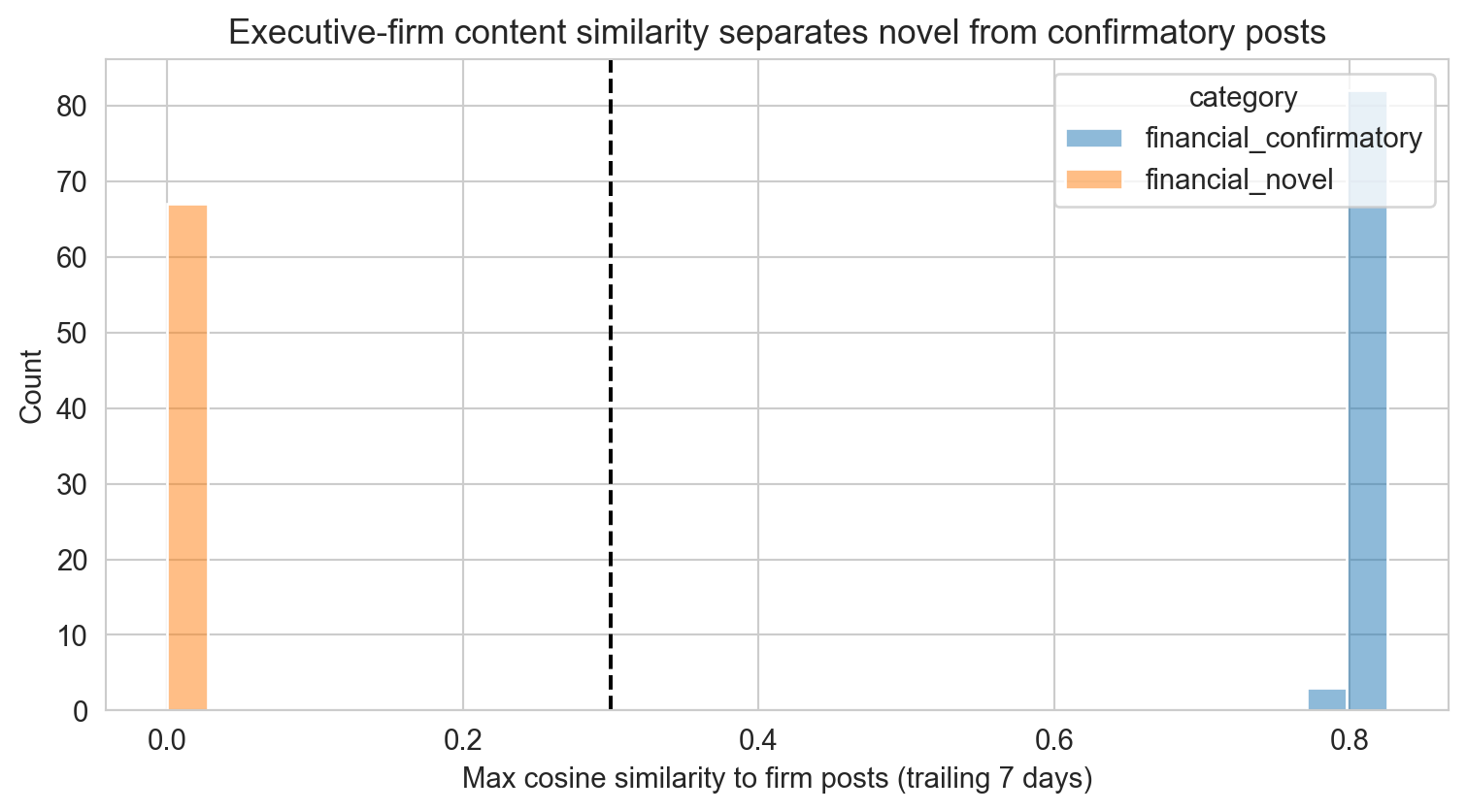
The core construct in Crowley, Huang, and Lu (2024b) is the content similarity between an executive’s post and the firm’s own recent posts, which converts the two market-reaction mechanisms into a measurable split: an executive financial post that closely resembles recent firm content is confirmatory (its reaction, if any, operates through credibility), while a financial post with no similar firm content is novel (its reaction reveals new information reaching the market through the executive). We implement the construct as the maximum cosine similarity between each executive financial post and the same firm’s official posts over the trailing seven calendar days, in a shared TF-IDF space (Section 53.1).
Executive-firm content similarity and novelty split
The similarity distribution is sharply bimodal: paraphrased earnings posts sit near the top of the range while guidance-like posts cluster near zero, so the split is not sensitive to the exact threshold. In production, the threshold should be validated against a manually labeled sample, and the TF-IDF space can be replaced by PhoBERT sentence embeddings (Section 53.2) to catch paraphrases that share meaning but not vocabulary.
55.4.5 Market Reactions to Executive Posts
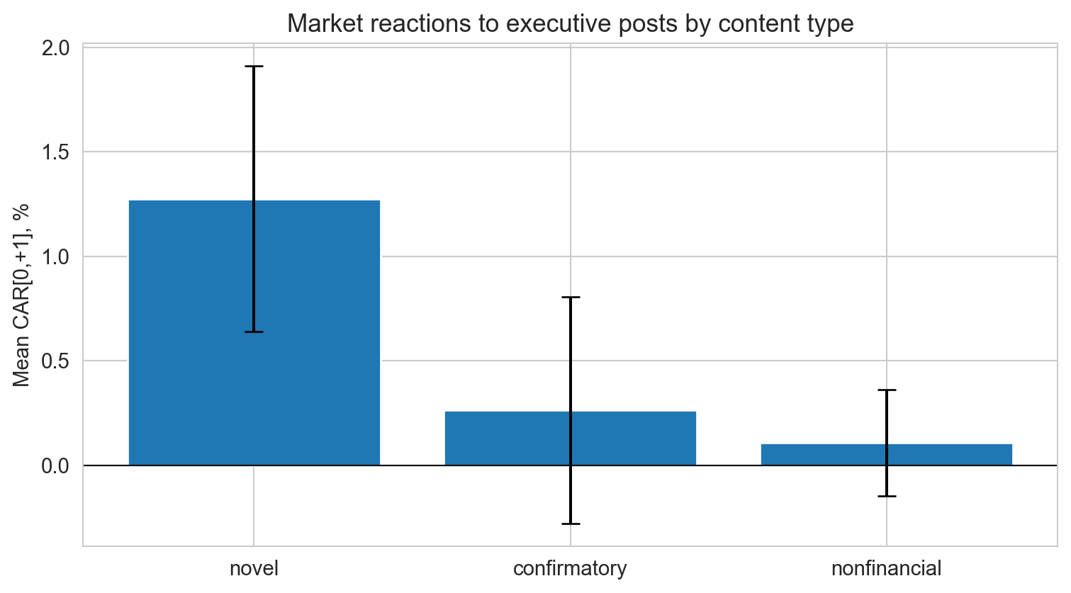
With posts classified and split, the market-reaction test follows the event-study logic: compute market-adjusted abnormal returns and cumulate them over the post window, separately for novel financial, confirmatory financial, and non-financial posts. Non-financial posts serve as the placebo, exactly as in Crowley, Huang, and Lu (2024b); if greetings and holiday wishes move prices, the design is contaminated.
The sandbox recovers the structure we embedded, which is also the structure Crowley, Huang, and Lu (2024b) find in actual US data: novel financial posts carry large and statistically significant reactions (the new-information channel), while non-financial posts are flat placebos. The confirmatory category is instructive in a different way: its embedded reaction is real but small, and at this simulated sample size it is not reliably distinguishable from zero, a reminder that credibility-channel effects require large post panels to detect (Crowley, Huang, and Lu (2024b) identify theirs from the full S&P 1500 tweet history), so a Vietnamese researcher should expect the novel-post result to emerge first and the confirmatory result to require accumulating years of data. On real Vietnamese data, this simple market-adjusted CAR should be replaced by the full inference machinery of the event studies chapter (risk-model abnormal returns, BMP and rank tests, and wider windows to respect price limits), and reactions should be measured in volume and volatility as well as returns, since retail-driven attention effects often appear in volume first.
55.4.6 From Replication to Production Monitoring
Everything above composes into a monitor that runs continuously: collect new posts, classify financial content, compute similarity against the firm’s official stream, and react within minutes rather than at the end of a research quarter. The skeleton below is deliberately thin; each method delegates to a component already built in this section.
Production: real-time executive post monitor
class ExecutiveSocialMonitor:"""Poll -> classify -> similarity -> alert, on a fixed schedule. Schedule with cron / Task Scheduler at the desired latency, e.g. every 5 minutes during HOSE trading hours (09:00-14:45 ICT). """def__init__(self, db_path, clf, clf_vectorizer, sim_vectorizer, sim_threshold=0.30, sim_window_days=7):self.db_path = db_pathself.clf, self.clf_vectorizer = clf, clf_vectorizerself.sim_vectorizer = sim_vectorizerself.sim_threshold = sim_thresholdself.sim_window_days = sim_window_daysdef poll(self):"""Collect new posts for every registered account (see exec-social-collection) and return those not yet processed.""" ...def classify(self, posts):"""Word-segment (underthesea), then flag financial content.""" ...def similarity(self, post):"""Max cosine similarity vs the firm's official posts in the trailing window; below threshold => novel.""" ...def alert(self, post, is_novel):"""Route by rule: - novel financial post by a covered executive -> analyst channel (candidate trading signal; log expected reaction window) - quantitative claim with no firm disclosure within 24h -> compliance flag (selective disclosure / manipulation risk) - deleted or edited financial post -> archive diff + escalate """ ...def run_once(self): new_posts =self.poll()for post inself.classify(new_posts):if post['is_financial']:self.alert(post, self.similarity(post) <self.sim_threshold)
Compliance and Ethics in the Vietnamese Setting
A production monitor must respect three constraints. First, collect only public business communications of public-company executives; Vietnam’s Personal Data Protection Decree (13/2023/NĐ-CP) and platform terms of service both bind, and private profiles are out of scope. Second, the same system that surfaces trading signals surfaces manipulation: executives or affiliated accounts posting inflated claims ahead of insider sales is exactly the pattern securities regulators sanction, so log everything immutably; the archive is evidence. Third, trading on a novel executive post is trading on public information the moment it is posted, but a researcher who receives material information privately from an executive is in different legal territory entirely. Jung et al. (2018) is the reminder that the observable stream is strategically selected; absence of posts is not absence of news.
Deployment Checklist
Registry: executive accounts verified from annual reports and governance disclosures; re-verify quarterly.
Collection: scheduled polling with immutable raw-JSON archive; deletion and edit tracking; UTC to ICT conversion; ATC-cutoff mapping to trading days.
Models: classifier retrained on a growing labeled set; similarity threshold re-validated; PhoBERT embeddings once paraphrase volume warrants it.
Measurement: CARs from the event studies chapter’s pipeline; volume and volatility reactions alongside returns.
Governance: compliance alerts routed separately from research alerts; quarterly review of false positive rates for both.
The research agenda this enables in Vietnam is largely unwritten: no published study yet measures whether Vietnamese executives’ Facebook and Zalo posts move the prices of their firms, how reactions differ across the retail-heavy HOSE investor base versus institutional holders, or whether the credibility mechanism of Crowley, Huang, and Lu (2024b) is stronger in a market where person-to-person trust plausibly substitutes for a thinner formal disclosure environment. The pipeline in this section is the infrastructure for all three questions.
Every representation built so far collapses a document into a single vector: a bag of words, an LDA mixture, a Doc2Vec paragraph vector, or an averaged PhoBERT embedding (Chapter 50, Section 51.1, Chapter 54). That is a reasonable choice for an annual report, where we care about what a firm says. It discards exactly the information that matters most in an earnings conference call, which is a conversation: the order in which topics arise, whether an analyst’s question returns to something management said earlier, and whether management volunteers a new subject. A mean-pooled embedding of a one-hour call is identical for two calls that discuss the same topics in very different ways.
Yang et al. (2026) propose to keep that structure. Their starting problem is that call transcripts are long and the risk-relevant signal is sparsely distributed across them, so models that compress a whole transcript into one vector tend to miss it. They instead model each transcript as a conversational graph whose nodes are discussed topics and whose edges link similar topics, so that the representation captures what is discussed (topical content), how it is discussed (cross-referencing earlier topics versus introducing new ones) and in what manner (sentiment and other linguistic features). A graph neural network (GNN) then learns a transcript-level representation for forecasting financial risk. The abstract reports four findings: forecast errors fall significantly relative to existing deep-learning and LLM baselines; the gain persists after controlling for firm fundamentals; the gain grows with transcript length; and, in the interpretability analysis, more cross-referencing, more newly introduced topics and a more positive tone are associated with lower subsequent risk. The paper appears in Information Systems Research 37(3), 1681–1705.
What this section does and does not replicate
I had access to the paper’s abstract and publication record, not its full text, so the code below is not a replication of the authors’ architecture, data or numbers. It implements the idea (transcript to topic graph to graph features and message passing to risk forecast) on simulated data, so that every step can be run and inspected. The graph neural network here has fixed random weights and a ridge readout; the authors train a GNN end to end. Treat the simulated results as a demonstration that the method can recover structure that pooled embeddings cannot, not as evidence about how large the gain is in real data.
55.5.1 A Simulation of Conversations with Structure
We generate 900 synthetic call transcripts. Each call has a number of turns (20 to 200, so length varies a lot) and a latent topic that evolves by a simple Markov rule: at each turn the discussion stays on the current topic, returns to a topic already raised with probability \(p_{\text{ref}}\) (a cross-reference), or opens a topic not yet raised with probability \(p_{\text{new}}\). Each turn is an embedding equal to its topic’s centroid plus noise (a stand-in for a PhoBERT sentence embedding), with a turn-level sentiment equal to the call’s tone plus noise. Next-period log volatility depends on three fundamentals (log size, leverage, past volatility) and, with the signs reported by Yang et al. (2026), negatively on \(p_{\text{ref}}\), \(p_{\text{new}}\) and tone. The point of the design is that \(p_{\text{ref}}\) and \(p_{\text{new}}\) are properties of the sequence of topics: they are invisible to any statistic that ignores turn order.
Simulate call transcripts as sequences of topic-labelled turns
from sklearn.cluster import KMeansfrom sklearn.linear_model import RidgeCVfrom sklearn.metrics import r2_scorecg_rng = np.random.default_rng(2026)CG_K, CG_D, CG_N =8, 16, 900cg_centroids = cg_rng.normal(0, 1, (CG_K, CG_D))def simulate_call(p_ref, p_new, tone, n_turns):"""One call: Markov topic path -> turn embeddings and turn sentiment.""" topic =int(cg_rng.integers(CG_K)) seen, path = [topic], [topic]for _ inrange(n_turns -1): u = cg_rng.random() unused = [k for k inrange(CG_K) if k notin seen]if u < p_new and unused: # introduce a new topic topic =int(cg_rng.choice(unused)); seen.append(topic)elif u < p_new + p_ref andlen(seen) >1: # cross-reference topic =int(cg_rng.choice([k for k in seen if k != topic])) path.append(topic) emb = cg_centroids[path] + cg_rng.normal(0, 0.8, (n_turns, CG_D)) sent = tone + cg_rng.normal(0, 0.8, n_turns)return emb, sentcg_firms = pd.DataFrame({'size': cg_rng.normal(size=CG_N), 'lev': cg_rng.normal(size=CG_N),'past_vol': cg_rng.normal(size=CG_N),'p_ref': cg_rng.uniform(0.05, 0.35, CG_N),'p_new': cg_rng.uniform(0.03, 0.20, CG_N),'tone': cg_rng.normal(0, 0.5, CG_N),'n_turns': np.clip(cg_rng.lognormal(4.0, 0.5, CG_N), 20, 200).astype(int),})cg_firms['y'] = (0.6* cg_firms.past_vol +0.15* cg_firms.lev-0.10* cg_firms['size']-6* cg_firms.p_ref -8* cg_firms.p_new -0.5* cg_firms.tone+ cg_rng.normal(0, 0.35, CG_N)) # next-period log volatilitycg_calls = [simulate_call(r.p_ref, r.p_new, r.tone, r.n_turns)for r in cg_firms.itertuples()]print(f'{CG_N} calls, {sum(len(c[1]) for c in cg_calls):,} turns; 'f'median length {int(cg_firms.n_turns.median())} turns')
900 calls, 55,938 turns; median length 54 turns
55.5.2 From Transcript to Graph
The graph builder has three steps. First, learn a corpus-level topic vocabulary by clustering all turn embeddings (here \(k\)-means; BERTopic, Section 51.2, is the natural production choice). Second, assign each turn to a topic; the distinct topics in a call become its nodes, with node features for topic share, mean sentiment, relative position of first mention and visit intensity, and edges between topics whose in-call centroids have high cosine similarity (the similarity edges of Yang et al. (2026)). Third, read off the graph and the discourse path. The new-topic rate is the number of nodes per turn. The cross-reference rate is the fraction of topic switches that return to an already-raised topic. We also compute a one-layer message-passing representation, \(\tanh(\hat{A}XW)\) mean-pooled over nodes, where \(\hat{A}\) is the symmetrically normalised adjacency with self-loops.
Build topic graphs and graph features per call
def call_graph(emb, sent, km, sim_threshold=0.3):"""Topic graph and discourse features for one call. emb: (turns, dim) turn embeddings; sent: (turns,) turn sentiment; km: fitted KMeans topic vocabulary. """ lab = km.predict(emb); L =len(lab) nodes =sorted(set(lab)) first = {k: int(np.argmax(lab == k)) for k in nodes} X = np.array([[np.mean(lab == k), sent[lab == k].mean(), first[k] / L, np.sum(lab == k) / L *len(nodes)] for k in nodes]) C = np.array([emb[lab == k].mean(0) for k in nodes]) Cn = C / np.linalg.norm(C, axis=1, keepdims=True) A = ((Cn @ Cn.T) > sim_threshold).astype(float) np.fill_diagonal(A, 1.0) d = A.sum(1); Ahat = A / np.sqrt(np.outer(d, d)) switches = np.flatnonzero(lab[1:] != lab[:-1]) +1 returns = [lab[t] inset(lab[:t]) for t in switches]returndict(X=X, Ahat=Ahat, new_rate=len(nodes) / L, xref=float(np.mean(returns)) iflen(switches) else0.0, switch_rate=len(switches) / L, density=(A.sum() -len(nodes)) /max(len(nodes) * (len(nodes) -1), 1), tone=sent.mean(), tone_sd=X[:, 1].std())cg_km = KMeans(CG_K, n_init=10, random_state=0).fit(np.vstack([c[0] for c in cg_calls]))cg_graphs = [call_graph(e, s, cg_km) for e, s in cg_calls]GRAPH_COLS = ['new_rate', 'xref', 'switch_rate', 'density', 'tone', 'tone_sd']F_graph = pd.DataFrame([{k: g[k] for k in GRAPH_COLS} for g in cg_graphs])cg_W = cg_rng.normal(0, 1, (4, 16)) # untrained message-passing weightsF_mp = np.array([np.tanh(g['Ahat'] @ g['X'] @ cg_W).mean(0) for g in cg_graphs])F_bag = np.column_stack([[c[0].mean(0) for c in cg_calls], F_graph.tone]) # pooled baselineprint(F_graph.assign(p_ref=cg_firms.p_ref, p_new=cg_firms.p_new) .corr().loc[['new_rate', 'xref'], ['p_new', 'p_ref']].round(2))
          p_new  p_ref
new_rate   0.51   0.01
xref       0.08   0.34
The correlations show that the observed graph statistics recover the latent discourse parameters: the new-topic rate tracks \(p_{\text{new}}\) and the cross-reference rate tracks \(p_{\text{ref}}\), even though topics are only estimated from noisy embeddings.
55.5.3 Does Structure Add Forecasting Power?
We mirror the paper’s “beyond fundamentals” logic: fit ridge regressions of next-period log volatility on (i) fundamentals only; (ii) fundamentals plus the pooled representation (mean embedding and mean tone); (iii) fundamentals plus the graph features; (iv) fundamentals plus message-passing features and tone. All models are fit on a 70% training split and scored out of sample, overall and by transcript-length tercile.
Out-of-sample comparison, overall and by transcript length
fund = cg_firms[['size', 'lev', 'past_vol']].valuestrain = cg_rng.random(CG_N) <0.7; test =~trainy = cg_firms.y.valuesdef fit_predict(X): X = np.asarray(X, float) mu, sd = X[train].mean(0), X[train].std(0) +1e-9 Z = (X - mu) / sdreturn RidgeCV(alphas=np.logspace(-2, 3, 20)).fit(Z[train], y[train]).predict(Z)specs = {'Fundamentals only': fund,'+ pooled embedding and tone': np.column_stack([fund, F_bag]),'+ graph features': np.column_stack([fund, F_graph]),'+ message passing': np.column_stack([fund, F_mp, F_graph.tone]),}tercile = pd.qcut(cg_firms.n_turns, 3, labels=['short', 'mid', 'long']).valuesrows = []for name, X in specs.items(): p = fit_predict(X) row = {'model': name, 'OOS R2': r2_score(y[test], p[test]),'RMSE': np.sqrt(np.mean((y[test] - p[test]) **2))}for t in ['short', 'mid', 'long']: m = test & (tercile == t) row[f'RMSE ({t})'] = np.sqrt(np.mean((y[m] - p[m]) **2)) rows.append(row)cg_results = pd.DataFrame(rows).set_index('model')base = cg_results.loc['Fundamentals only']gain =1- cg_results.filter(like='RMSE (').div(base.filter(like='RMSE ('))print(cg_results.round(3).to_string())print('\nRMSE reduction vs fundamentals-only, by call length:')print(gain.round(3).to_string())
                             OOS R2   RMSE  RMSE (short)  RMSE (mid)  RMSE (long)
model
Fundamentals only             0.379  0.811         0.794       0.896        0.737
+ pooled embedding and tone   0.407  0.792         0.773       0.881        0.716
+ graph features              0.629  0.626         0.729       0.668        0.453
+ message passing             0.491  0.734         0.744       0.792        0.663

RMSE reduction vs fundamentals-only, by call length:
                             RMSE (short)  RMSE (mid)  RMSE (long)
model
Fundamentals only                   0.000       0.000        0.000
+ pooled embedding and tone         0.025       0.016        0.028
+ graph features                    0.081       0.254        0.385
+ message passing                   0.062       0.116        0.100
Three patterns appear, all of which are built into the simulation, so they validate the machinery and are not evidence about real markets. The pooled baseline adds almost nothing, because averaging embeddings cannot see turn order. The graph features add a great deal, because \(p_{\text{ref}}\) and \(p_{\text{new}}\) are structural. The RMSE reduction is larger for long calls, because a long call contains more turns from which to estimate the call’s discourse rates; this is one mechanical route to the length gradient that Yang et al. (2026) report, though their data may generate it through other channels, such as the sparse-signal problem for models that pool a long transcript. The untrained message-passing representation helps less than the hand-built graph features, which is a reminder that the paper’s gain comes from training the network on the structure and not from the architecture label.
55.5.4 Production Application with DataCore.vn
The production version swaps the simulated turns for real call transcripts. The cell below is a skeleton: get_earnings_call_transcripts follows the chapter’s DataCore conventions for text retrieval, and the helper embed_turns should use the PhoBERT sentence encoder of Section 54.1 on word-segmented turns (Section 49.1). It reuses call_graph from above unchanged, which is the point of keeping that function dependent only on turn embeddings and turn sentiment.
Production: Vietnamese earnings call graphs and volatility forecast
# Transcripts: one row per speaker turn (ticker, call_date, turn_idx, role, text)turns = dc.get_earnings_call_transcripts(start='2018-01-01', end='2024-12-31')turns = turns.sort_values(['ticker', 'call_date', 'turn_idx'])# Turn embeddings (PhoBERT sentence encoder) and sentiment (see sec-textual-bert-sentiment)turns['emb'] =list(embed_turns(turns['text_segmented']))turns['sent'] = sentiment_score(turns['text_segmented'])# Corpus-level topic vocabulary: fit on the training period onlytrain_turns = turns[turns.call_date <'2022-01-01']topic_km = KMeans(30, n_init=10, random_state=0).fit(np.vstack(train_turns['emb']))rows = []for (tic, dt), g in turns.groupby(['ticker', 'call_date']): feats = call_graph(np.vstack(g['emb']), g['sent'].values, topic_km) rows.append({'ticker': tic, 'call_date': dt, 'n_turns': len(g),**{k: feats[k] for k in GRAPH_COLS}})graph_df = pd.DataFrame(rows)# Target: realised volatility over the 21 trading days after the call (skip day 0)vol = dc.get_realized_volatility(window=21, offset=1)fundamentals = dc.get_fundamentals(['log_size', 'leverage', 'past_vol'])panel = (graph_df.merge(vol, on=['ticker', 'call_date']) .merge(fundamentals, on=['ticker', 'call_date']))# Same split-by-time ridge comparison as the simulation, with time-based train/test
55.5.5 Vietnam-Specific Research Design
Applying this design in Vietnam changes the problem in four ways.
Data are the binding constraint. Quarterly earnings calls are a US institution. Vietnamese listed firms mostly communicate through filed reports, annual general meetings (AGMs, Đại hội đồng cổ đông), investor-relations presentations and analyst roadshows, with call transcripts available for only a fraction of larger HOSE names. The same graph construction applies to any multi-party dialogue: the Q&A part of an AGM, an analyst roadshow Q&A, or a broker-hosted corporate access day. Start by counting how many firm-quarters have a usable transcript before designing anything else.
Replace the topic vocabulary and the sentiment measure. Fit the topic model on Vietnamese financial text with word-segmented input (Section 49.1) and use ViFinBERT or the dictionary of Section 52.1 for tone. A topic vocabulary fit on the full sample leaks future information, so fit it on the training period only, as in the code above.
Choose the target to match market structure. The paper’s target is financial risk. For Vietnam, use post-call realised volatility, but note the daily price limits of \(\pm 7\%\) (HOSE), \(\pm 10\%\) (HNX) and \(\pm 15\%\) (UPCoM), which truncate return-based risk on event days; a high-low range measure or a multi-day window is less affected. Control for foreign ownership room and retail turnover share, which drive volatility independently of what is said.
Interpretation beyond prediction. The paper’s finding that cross-referencing, new topics and a positive tone coincide with lower risk is a statement about predictive association. In a retail-heavy market, where managers know the audience is less specialised, the same patterns could reflect managerial choices (a scripted call that avoids new topics) and not underlying fundamentals. Compare calls with and without independent analyst participation, and test whether the new-topic rate reflects analyst questions (exogenous to management) or management’s own agenda.
A practical research design therefore: (a) assemble all Vietnamese transcripts and estimate coverage by size tercile; (b) construct topic graphs and the discourse features above; (c) run the nested comparison of fundamentals, pooled text and graph features out of sample on a rolling time split; and (d) report the length gradient, which is the most informative diagnostic for whether structure matters in this market.
55.6 Earnings Calls in Regulatory Review
The previous section treats an earnings call as a signal for investors. Lerman, Steffen, and Zhang (2026) show that the regulator reads the same transcripts. The SEC’s Division of Corporation Finance reviews every registrant’s periodic filings at least once every three years and sends comment letters when it finds deficiencies in disclosure or accounting. The letters and the firms’ responses become public after the review closes. Lerman, Steffen and Zhang hand-collect the comment letters that cite what management said on a voluntary earnings conference call. They then ask three questions: what the SEC uses that information for, when it does so, and what changes afterwards.
Their sample covers a little over 800 letters from 2005 to 2018, slightly more than 1% of all comment-letter conversations. Most come from reviews of 10-K filings (over two-thirds) and 10-Q filings (18%).4 The main findings are:
Calls are a benchmark for mandatory filings. In about 80% of the letters the SEC cites the call to show that the 10-K or 10-Q says too little: management discussed a driver, metric or segment on the call that the filing omits. About 15% point to inconsistencies between the call and the filing. Few letters criticise the call itself, except for its use of non-GAAP measures. Revenue, segment reporting, and non-GAAP measures or KPIs together make up about 45% of the sample, and MD&A topics (risk factors, products, customers, markets, seasonality) another 23%.
Determinants. Call-referencing letters are more likely when the filing review is more complex (larger review teams with more accountants), when SEC staff are less resource constrained, and for firms with more institutional investors and analyst following. These are the firms whose calls are most closely followed.
Remediation costs. These letters occur during higher-quality reviews. They raise more issues per conversation, need more rounds of correspondence, and take longer to reach “no further comment” than other letters.
Consequences. Firms change their subsequent mandatory filings more after a call-referencing letter, especially when they agree with the comment. The filings get longer, more negative in tone, and use more uncertain and constraining words as measured by the Loughran and McDonald (2011) word lists. The effect on the wider information environment is mixed: bid-ask spreads and illiquidity rise. This fits an unintended consequence: once managers learn that the regulator reads the call, the call itself may become less informative.
For a textual-analysis chapter, the paper makes three points. First, the regulator is doing cross-document comparison by hand: it holds the call next to the filing and looks for content in one that is missing from, or contradicts, the other. This is a measurable construct. Second, call language responds to enforcement. Models that treat call text as unconstrained managerial communication (Section 55.5) should allow for the fact that what managers say is shaped by who is listening. Third, the outcome measures are standard dictionary counts (Section 52.1) applied to filings, so the paper also shows how tone measures serve as dependent variables, not only as return predictors.
A scalable version of the regulator’s comparison is a call-to-filing coverage gap. This measure is our suggestion; the paper itself codes letters by hand. Let \(S^{\text{call}}_{it}\) be the sentences of firm \(i\)’s call for period \(t\) and \(S^{\text{file}}_{it}\) the sentences of the subsequent periodic report, each embedded as \(e_s\) with a sentence encoder (Section 53.2). Then
the share of call sentences with no close counterpart in the filing. Restrict \(S^{\text{call}}_{it}\) to sentences that carry hard information (numbers, segment names, KPI terms), because the SEC’s “insufficiency” comments target exactly these. Choose \(\tau\) by hand-labelling a validation sample of matched and unmatched pairs. Inconsistencies are harder to detect: within matched sentence pairs, extract the numbers with their units and flag pairs whose values disagree.
55.6.1 Vietnam-Specific Research Design
The US design does not transplant directly, because Vietnam has no public comment-letter process. The State Securities Commission (SSC, Ủy ban Chứng khoán Nhà nước) does not publish its review correspondence. The voluntary channel also differs: quarterly earnings calls are held by only a minority of large caps, while AGMs, investor-relations presentations and analyst meetings carry most voluntary disclosure (Section 55.5.5). What does exist publicly are several “regulator meets disclosure” records:
Mandated profit explanations. Under Circular 96/2020/TT-BTC, listed firms must publish an explanation (giải trình) when after-tax profit changes by 10% or more year on year or swings from profit to loss, and when audited profit differs by 5% or more from the pre-audit figure. The pre-audit versus audited gap is the closest local analogue to the SEC’s “inconsistency” comments, and it is filed as text on the HOSE and HNX disclosure portals.
Enforcement outcomes. SSC administrative sanction decisions for disclosure violations are published, and the exchanges place stocks on warning or control lists for late filings or modified audit opinions. These are noisier than comment letters but play the same role as the outcome variable.
Auditor modifications. Qualified opinions and emphasis-of-matter paragraphs are a third party’s “comment” on the filing and can be dated precisely.
Research designs that follow from this:
Voluntary-to-mandatory gap as a predictor. Compute Equation 55.2 with AGM minutes or IR presentations in place of the call, and the annual report or MD&A in place of the 10-K. Test whether a larger gap predicts a later profit explanation, a pre-audit to audited revision of 5% or more, a modified audit opinion, or an SSC sanction.
Who gets scrutinised. In the US, call-referencing letters concentrate on firms with institutional and analyst following. In Vietnam, foreign institutional ownership is concentrated in large caps, while enforcement has targeted manipulation in retail-heavy small caps, as in the 2022 FLC and Tân Hoàng Minh cases. Expect a different determinant structure, and test it before assuming the US pattern.
Chilling effect on voluntary disclosure. The paper’s mixed information-environment result suggests testing whether firms (or industry peers) say less in AGM Q&A or IR materials after a sanction or a visible enforcement wave. Measure this with transcript length, the share of sentences with numbers, and the forward-looking word share. Compare with firms that were not exposed.
Bilingual consistency. Larger listed firms publish both Vietnamese and English versions of their reports. Apply the same gap measure across languages with a multilingual encoder. Divergence between the two versions is a Vietnam-specific inconsistency that foreign investors may price.
56 Method Comparison and Best Practices
Table 56.1: Comparison of Textual Analysis Methods for Vietnamese Financial Text
Method
Interpretability
Semantic
Speed
VN Support
Data Req.
Best Use Case
BoW/TF-IDF
High
Low
Fast
Good*
None
Peer groups, lexical similarity
LDA
Medium
Low
Medium
Good*
None
Topic discovery
Doc2Vec
Low
Medium
Medium
Good*
Corpus
Document similarity
BERTopic
High
High
Slow
Excellent
None
Coherent topics
PhoBERT
Low
High
Slow
Excellent
Fine-tune
Sentiment, NER, classification
Sentence-BERT
Low
High
Medium
Good
None
Semantic similarity
LLM (zero-shot)
High
High
Slow
Good
None
Extraction, classification
Note
*Requires Vietnamese word segmentation as a preprocessing step. VN Support rates how well the method handles Vietnamese text natively.
For researchers beginning textual analysis of Vietnamese firms, we recommend the following workflow:
Start with TF-IDF cosine similarity for peer identification because it is fast, interpretable, and provides a strong baseline.
Use BERTopic with PhoBERT embeddings for topic discovery because it produces more coherent topics than LDA for Vietnamese text.
For sentiment analysis, use ViFinBERT if fine-tuning data is available; otherwise, LLM zero-shot classification provides competitive results.
For production systems requiring real-time analysis, sentence-BERT embeddings offer the best speed-accuracy tradeoff.
Compare methods on peer identification accuracy
# Evaluate: what fraction of top-5 peers share ICB sector?methods = {'TF-IDF': sim_df,'Sentence-BERT': embed_sim_df,'Doc2Vec': pd.DataFrame( cosine_similarity(d2v_vectors), index=tickers, columns=tickers ),}accuracy_results = {}sector_map = corpus_df.set_index('ticker')['icb_sector'].to_dict()for method_name, sim_matrix_df in methods.items(): matches =0 total =0for ticker in tickers: true_sector = sector_map.get(ticker) peers = sim_matrix_df[ticker].drop(ticker).nlargest(5)for peer in peers.index: total +=1if sector_map.get(peer) == true_sector: matches +=1 accuracy_results[method_name] = matches / totalfig, ax = plt.subplots(figsize=(8, 5))methods_list =list(accuracy_results.keys())accs =list(accuracy_results.values())bars = ax.bar(methods_list, accs, color=['#2C5282', '#38A169', '#D69E2E'])ax.set_ylabel('ICB Sector Match Rate')ax.set_title('Peer Identification Accuracy by Method')ax.set_ylim(0, 1)for bar, acc inzip(bars, accs): ax.text(bar.get_x() + bar.get_width()/2., bar.get_height() +0.02,f'{acc:.1%}', ha='center', fontweight='bold')plt.tight_layout()plt.show()
Figure 56.1
57 Conclusion
This chapter worked through the full pipeline of textual analysis methods applied to Vietnamese listed firms, from classical bag-of-words approaches to transformer-based language models. The key takeaways for practitioners and researchers are:
First, Vietnamese text preprocessing requires a word segmentation step that has no parallel in English-language NLP. Using tools like VnCoreNLP or underthesea for this step is essential and significantly affects downstream analysis quality.
Second, domain-specific sentiment lexicons substantially outperform general-purpose dictionaries for Vietnamese financial text, consistent with Loughran and McDonald (2011) findings for English.
Third, PhoBERT-based embeddings capture semantic similarity that TF-IDF misses, identifying industry peers that share business models even when they use different vocabulary.
Fourth, LLMs enable new applications, including structured information extraction from Vietnamese annual reports that would be prohibitively expensive with manual coding.
The empirical applications demonstrate that textual measures contain economically meaningful information for the Vietnamese market. Net sentiment from annual reports predicts subsequent stock returns even after controlling for standard risk factors, and BERT-based sentiment measures have incremental predictive power beyond dictionary-based measures. Text-based industry classifications capture firm relationships that static ICB codes miss, and textual similarity changes around corporate events reflect real business transformations.
Bartov, Eli, Lucile Faurel, and Partha S Mohanram. 2018. “Can Twitter Help Predict Firm-Level Earnings and Stock Returns?”The Accounting Review 93 (3): 25–57.
Blankespoor, Elizabeth, Gregory S Miller, and Hal D White. 2014. “The Role of Dissemination in Market Liquidity: Evidence from Firms’ Use of Twitter.”The Accounting Review 89 (1): 79–112.
Blei, David M, Andrew Y Ng, and Michael I Jordan. 2003. “Latent Dirichlet Allocation.”Journal of Machine Learning Research 3 (Jan): 993–1022.
Bonsall IV, Samuel B, Andrew J Leone, Brian P Miller, and Kristina Rennekamp. 2017. “A Plain English Measure of Financial Reporting Readability.”Journal of Accounting and Economics 63 (2-3): 329–57.
Bybee, Leland, Bryan Kelly, and Yinan Su. 2023. “Narrative Asset Pricing: Interpretable Systematic Risk Factors from News Text.”The Review of Financial Studies 36 (12): 4759–87.
Chen, Hailiang, Prabuddha De, Yu Jeffrey Hu, and Byoung-Hyoun Hwang. 2014. “Wisdom of Crowds: The Value of Stock Opinions Transmitted Through Social Media.”The Review of Financial Studies 27 (5): 1367–1403.
Crowley, Richard M, Wenli Huang, and Hai Lu. 2024a. “Discretionary Dissemination on Twitter.”Contemporary Accounting Research 41 (4): 2454–87.
Devlin, Jacob, Ming-Wei Chang, Kenton Lee, and Kristina Toutanova. 2019. “Bert: Pre-Training of Deep Bidirectional Transformers for Language Understanding.” In Proceedings of the 2019 Conference of the North American Chapter of the Association for Computational Linguistics: Human Language Technologies, Volume 1 (Long and Short Papers), 4171–86.
Dyer, Travis, Mark Lang, and Lorien Stice-Lawrence. 2017. “The Evolution of 10-k Textual Disclosure: Evidence from Latent Dirichlet Allocation.”Journal of Accounting and Economics 64 (2-3): 221–45.
Grootendorst, Maarten. 2022. “BERTopic: Neural Topic Modeling with a Class-Based TF-IDF Procedure.”arXiv Preprint arXiv:2203.05794.
Hoberg, Gerard, and Gordon Phillips. 2010. “Product Market Synergies and Competition in Mergers and Acquisitions: A Text-Based Analysis.”The Review of Financial Studies 23 (10): 3773–3811.
———. 2016. “Text-Based Network Industries and Endogenous Product Differentiation.”Journal of Political Economy 124 (5): 1423–65. https://doi.org/10.1086/688176.
Hoberg, Gerard, and Gordon M Phillips. 2018. “Text-Based Industry Momentum.”Journal of Financial and Quantitative Analysis 53 (6): 2355–88.
Huang, Allen H, Reuven Lehavy, Amy Y Zang, and Rong Zheng. 2018. “Analyst Information Discovery and Interpretation Roles: A Topic Modeling Approach.”Management Science 64 (6): 2833–55.
Huang, Allen H, Hui Wang, and Yi Yang. 2023. “FinBERT: A Large Language Model for Extracting Information from Financial Text.”Contemporary Accounting Research 40 (2): 806–41.
Jha, Manish, Jialin Qian, Michael Weber, and Baozhong Yang. 2024. “ChatGPT and Corporate Policies.” National Bureau of Economic Research.
Jung, Michael J, James P Naughton, Ahmed Tahoun, and Clare Wang. 2018. “Do Firms Strategically Disseminate? Evidence from Corporate Use of Social Media.”The Accounting Review 93 (4): 225–52.
Lau, Jey Han, and Timothy Baldwin. 2016. “An Empirical Evaluation of Doc2vec with Practical Insights into Document Embedding Generation.”arXiv Preprint arXiv:1607.05368.
Le, Quoc, and Tomas Mikolov. 2014. “Distributed Representations of Sentences and Documents.” In International Conference on Machine Learning, 1188–96. PMLR.
Lerman, Alina, Thomas D. Steffen, and Kangkang Zhang. 2026. “Earnings Conference Calls and the SEC Comment Letter Process.”Management Science 72 (10): 8571–8604. https://doi.org/10.1287/mnsc.2023.02065.
Li, Feng et al. 2010. “Textual Analysis of Corporate Disclosures: A Survey of the Literature.”Journal of Accounting Literature 29 (1): 143–65.
Loughran, Tim, and Bill McDonald. 2011. “When Is a Liability Not a Liability? Textual Analysis, Dictionaries, and 10-Ks.”The Journal of Finance 66 (1): 35–65.
Nguyen, Dat Quoc, and Anh-Tuan Nguyen. 2020. “PhoBERT: Pre-Trained Language Models for Vietnamese.” In Findings of the Association for Computational Linguistics: EMNLP 2020, 1037–42.
Reimers, Nils, and Iryna Gurevych. 2019. “Sentence-Bert: Sentence Embeddings Using Siamese Bert-Networks.”arXiv Preprint arXiv:1908.10084.
Tetlock, Paul C. 2007. “Giving Content to Investor Sentiment: The Role of Media in the Stock Market.”The Journal of Finance 62 (3): 1139–68.
Tetlock, Paul C, Maytal Saar-Tsechansky, and Sofus Macskassy. 2008. “More Than Words: Quantifying Language to Measure Firms’ Fundamentals.”The Journal of Finance 63 (3): 1437–67.
Vu, Thanh, Dat Quoc Nguyen, Mark Dras, Mark Johnson, et al. 2018. “VnCoreNLP: A Vietnamese Natural Language Processing Toolkit.” In Proceedings of the 2018 Conference of the North American Chapter of the Association for Computational Linguistics: Demonstrations, 56–60.
Yang, Yi, Yixuan Tang, Yangyang Fan, and Kunpeng Zhang. 2026. “Learning from Earnings Calls: Graph-Based Conversational Modeling for Financial Prediction.”Information Systems Research 37 (3): 1681–1705. https://doi.org/10.1287/isre.2023.0519.
Vietnamese text requires specialized tokenization due to compound words (e.g., “công ty” = company, “thị trường” = market).↩︎
Loughran and McDonald (2011) show that general-purpose dictionaries misclassify up to 73% of negative words in financial text.↩︎
Reimers and Gurevych (2019) demonstrate that sentence-BERT embeddings reduce computation for similarity tasks from 65 hours to 5 seconds on 10,000 sentence pairs.↩︎
Sample sizes and percentages in this section come from the authors’ summary of the working-paper version (CLS Blue Sky Blog, July 2023). The qualitative findings match the published abstract.↩︎
Source Code
# Textual AnalysisTextual analysis has emerged as one of the most productive research frontiers in empirical finance over the past two decades. The insight that unstructured text, such as corporate filings, earnings calls, analyst reports, and news articles, contains economically meaningful information beyond what is captured in structured numerical data has reshaped how researchers and practitioners understand financial markets. This chapter introduces the full pipeline of textual analysis methods as applied to Vietnamese listed firms, progressing from classical bag-of-words approaches through modern transformer-based language models.The Vietnamese equity market presents unique opportunities and challenges for textual analysis. As of 2024, the Ho Chi Minh Stock Exchange (HOSE) and the Hanoi Stock Exchange (HNX) together list over 1,600 securities with a combined market capitalization exceeding VND 6,000 trillion (approximately USD 240 billion). Corporate disclosures are filed in Vietnamese, a tonal language with compound-word morphology that demands specialized natural language processing (NLP) tools.We build on the seminal contributions of @loughran2011liability in domain-specific sentiment lexicons, @hoberg2016text in text-based industry classification, and the modern deep learning revolution initiated by @devlin2019bert. This chapter covers the following topics:1. Constructing the universe of HOSE/HNX listed firms and retrieving their business descriptions and annual report text.2. Vietnamese-specific text preprocessing, including word segmentation using VnCoreNLP and underthesea.3. Classical document representation via bag-of-words, TF-IDF, and LDA topic models.4. Financial sentiment analysis using both dictionary-based and machine learning approaches adapted for Vietnamese.5. Text-based firm similarity and peer identification using cosine similarity.6. Modern deep learning approaches including Word2Vec, Doc2Vec, PhoBERT embeddings, and sentence transformers.7. Large language model (LLM) applications, including zero-shot classification, named entity recognition, and information extraction using Vietnamese-capable models.8. Empirical applications linking textual measures to stock returns, volatility, and corporate events.## Why Textual Analysis for Vietnamese Finance? {#sec-textual-why-vietnam}The Vietnamese financial market has several characteristics that make textual analysis particularly valuable. First, analyst coverage is sparse (fewer than 30% of listed firms receive regular coverage from sell-side analysts), making alternative information sources critical. Second, the regulatory environment is evolving rapidly, with the State Securities Commission (SSC) continuously updating disclosure requirements, creating rich variation in information environments across firms and time. Third, the market is dominated by retail investors (accounting for roughly 80% of trading volume), who may process textual information differently than institutional investors, creating potential mispricings that text-based strategies could exploit.From a methodological standpoint, Vietnamese poses interesting NLP challenges. Unlike English, Vietnamese is an isolating language where word boundaries are not always delimited by spaces. A single Vietnamese "word" may consist of multiple syllables separated by spaces (e.g., "công ty" for "company," "thị trường" for "market"). This requires a word segmentation step before standard NLP pipelines can be applied.[^60_textual-1][^60_textual-1]: Vietnamese text requires specialized tokenization due to compound words (e.g., "công ty" = company, "thị trường" = market).# Literature Review {#sec-textual-literature}## Textual Analysis in Finance {#sec-textual-lit-finance}The application of textual analysis to financial data has a rich history. @tetlock2007giving demonstrated that the pessimism content of a Wall Street Journal column predicts aggregate market activity, providing early evidence that textual content moves prices. @loughran2011liability showed that the widely-used Harvard General Inquirer sentiment dictionary produces misleading results when applied to financial text because words like "liability," "tax," and "capital" are classified as negative in general English but carry neutral or even positive connotations in finance. Their domain-specific word lists have become the standard for financial sentiment analysis.[^60_textual-2][^60_textual-2]: @loughran2011liability show that general-purpose dictionaries misclassify up to 73% of negative words in financial text.@hoberg2010product and @hoberg2016text pioneered the use of product descriptions from 10-K filings to construct text-based industry classifications (TNIC), demonstrating that these dynamic, firm-specific industry definitions outperform static SIC and NAICS codes in explaining firm behavior, including profitability, stock returns, and M&A activity. Subsequent work by @hoberg2018text extended this to assess competitive threats and product-market fluidity.More recent work has leveraged advances in deep learning. @huang2023finbert apply BERT-based models to earnings call transcripts and show that contextual embeddings capture information about future earnings that traditional bag-of-words measures miss. @jha2024chatgpt use GPT-based models for zero-shot financial text classification and demonstrate that LLMs can match or exceed purpose-built classifiers on standard benchmarks. Earnings calls are also read by regulators: @lerman2026earnings show that the SEC cites voluntary call disclosures in comment letters, mostly to show that the mandatory filing says too little, and that firms then change their filings (@sec-textual-call-sec-review).Text can also measure the *uncertainty* investors face, not only its tone. @wei2026narrative extract a narrative-based ambiguity measure from economic news articles, distinct from survey- and return-based ambiguity proxies, and show that it predicts aggregate stock market returns both in and out of sample. Investors are on average ambiguity averse, but ambiguity tolerance emerges when the probability of loss is high, and aligning industry-specific narrative ambiguity (chiefly from consumption-, energy-, and technology-related news) yields a stronger market predictor. The predictability extends to international markets and other asset classes, which makes the approach a natural candidate for Vietnamese financial news.## NLP for Vietnamese Language {#sec-textual-lit-vnlp}Vietnamese NLP has advanced significantly with the development of VnCoreNLP [@vu2018vncorenlp], a Java-based toolkit providing word segmentation, POS tagging, named entity recognition, and dependency parsing. The underthesea library offers a Python-native alternative. Most critically for financial applications, PhoBERT [@nguyen2020phobert] provides Vietnamese-specific BERT pre-training on a 20GB corpus, achieving state-of-the-art results on multiple Vietnamese NLP tasks.| Study | Method | Key Finding | Relevance to Vietnam ||:-----------------|:-----------------|:-----------------|:------------------|| @tetlock2007giving | Dictionary-based sentiment from WSJ column | Media pessimism predicts market activity and returns | Baseline for Vietnamese financial news sentiment || @loughran2011liability | Domain-specific financial dictionaries | General dictionaries misclassify 73% of negative financial words | Need for Vietnamese financial sentiment lexicon || @hoberg2016text | Cosine similarity on 10-K product descriptions | Text-based industries outperform SIC/NAICS | Peer identification for Vietnamese firms using business descriptions || @nguyen2020phobert | PhoBERT: Vietnamese BERT pre-training | SOTA on Vietnamese NLP benchmarks | Foundation model for Vietnamese financial NLP || @huang2023finbert | BERT embeddings on earnings calls | Contextual embeddings predict future earnings beyond BoW | Apply to Vietnamese earnings call transcripts || @jha2024chatgpt | GPT-based zero-shot financial classification | LLMs match fine-tuned classifiers | Zero-shot Vietnamese financial text classification via multilingual LLMs || @wei2026narrative | Narrative ambiguity extracted from economic news | News-based ambiguity predicts market returns beyond survey- and return-based measures; aversion turns to tolerance at high loss probability | Aggregate ambiguity index from Vietnamese financial news for VN-Index return predictability || @crowley2024executive | ML classification + content similarity of S&P 1500 executives' tweets | Investors react to executives' financial tweets through both new-information and credibility channels | Executive Facebook/Zalo posts of Vietnamese listed firms (@sec-textual-exec-social) |: Key Literature on Textual Analysis in Finance {#tbl-literature}# Data: Vietnamese Listed Firms from DataCore.vn {#sec-textual-data}## Constructing the Universe {#sec-textual-universe}We construct the universe of Vietnamese listed firms. The universe includes all firms listed on HOSE, HNX, and UPCoM as of the analysis date.```{python}#| label: setup#| code-summary: "Import required libraries"import pandas as pdimport numpy as npimport reimport unicodedataimport warningsimport matplotlib.pyplot as pltimport seaborn as snsfrom collections import defaultdictfrom typing import List, Dict, Tuple, Optionalwarnings.filterwarnings('ignore')np.random.seed(42)# Plotting configurationplt.rcParams['figure.figsize'] = (10, 6)plt.rcParams['font.size'] =11sns.set_style("whitegrid")``````{python}#| label: build-universe#| eval: false#| code-summary: "Connect to DataCore.vn and build universe of listed firms"from datacore import DataCoreAPI # DataCore.vn Python client# Initialize connectiondc = DataCoreAPI(api_key='YOUR_API_KEY')# Retrieve universe of all listed firmsuniverse = dc.get_listed_firms( exchanges=['HOSE', 'HNX', 'UPCOM'], as_of='2024-12-31', fields=['ticker', 'company_name', 'company_name_en','exchange', 'listing_date', 'delisting_date','icb_industry', 'icb_sector', 'icb_subsector','market_cap', 'total_assets', 'revenue' ])print(f'Total listed firms: {len(universe)}')print(f'HOSE: {len(universe[universe.exchange=="HOSE"])}')print(f'HNX: {len(universe[universe.exchange=="HNX"])}')print(f'UPCoM: {len(universe[universe.exchange=="UPCOM"])}')```| Exchange | N Firms | Avg Mkt Cap (VND bn) | Median Mkt Cap (VND bn) | Total Mkt Cap (VND tn) ||:--------------|--------------:|--------------:|--------------:|--------------:|| HOSE | 403 | 12,847 | 3,215 | 5,177 || HNX | 334 | 2,156 | 687 | 720 || UPCoM | 868 | 1,043 | 298 | 905 || **Total** | **1,605** | **4,239** | **712** | **6,802** |: Universe of Vietnamese Listed Firms by Exchange (as of December 2024) {#tbl-universe}## Retrieving Business Descriptions {#sec-textual-bus-desc}Business descriptions for all listed firms can be in both Vietnamese and English. We retrieve both versions for our analysis. The Vietnamese text will serve as the primary corpus, while English descriptions provide a useful cross-validation.```{python}#| label: get-bus-desc#| eval: false#| code-summary: "Retrieve business descriptions."# Get business descriptions (Vietnamese and English)bus_desc = dc.get_business_descriptions( tickers=universe.ticker.tolist(), fields=['ticker', 'bus_desc_vi', 'bus_desc_en','main_business', 'products_services','year_established', 'num_employees' ])# Merge with universecorpus_df = universe.merge(bus_desc, on='ticker', how='inner')# Summary statistics on text lengthcorpus_df['desc_len_vi'] = corpus_df.bus_desc_vi.str.len()corpus_df['desc_len_en'] = corpus_df.bus_desc_en.str.len()corpus_df['word_count_vi'] = corpus_df.bus_desc_vi.str.split().str.len()print(corpus_df[['desc_len_vi', 'desc_len_en', 'word_count_vi']] .describe().round(0))```| Statistic | Mean | Median | Std Dev | Min | Max ||:----------------|------:|-------:|--------:|----:|-------:|| Characters (VN) | 2,847 | 2,156 | 1,923 | 87 | 18,432 || Characters (EN) | 3,412 | 2,689 | 2,245 | 102 | 22,156 || Words (VN) | 487 | 372 | 318 | 15 | 3,216 |: Descriptive Statistics of Business Description Text {#tbl-desc-stats}## Retrieving Annual Report Text {#sec-textual-annual-text}Beyond business descriptions, annual or quarterly reports provide richer and more time-varying textual data. We extract the Management Discussion and Analysis (MD&A) sections, which are most informative for financial analysis [@li2010textual; @bonsall2017plain]. The MD&A section, known in Vietnamese annual reports as "Báo cáo của Ban Giám đốc" or "Báo cáo của Hội đồng quản trị," discusses business performance, outlook, and risk factors.```{python}#| label: get-annual-text#| eval: false#| code-summary: "Retrieve annual report MD&A sections"# Get annual report MD&A sections (2015-2024)annual_text = dc.get_annual_report_text( tickers=universe.ticker.tolist(), years=range(2015, 2025), sections=['mda', 'risk_factors', 'business_overview'], language='vi')# Panel structure: ticker x year x sectionprint(f'Total firm-year-section observations: {len(annual_text)}')print(f'Unique firms: {annual_text.ticker.nunique()}')print(f'Year range: {annual_text.year.min()}-{annual_text.year.max()}')# Calculate text changes year-over-yearannual_text = annual_text.sort_values(['ticker', 'year'])annual_text['text_len'] = annual_text.text.str.len()annual_text['text_change_pct'] = ( annual_text.groupby('ticker')['text_len'] .pct_change() *100)```# Text Preprocessing for Vietnamese {#sec-textual-preprocessing}## Vietnamese Word Segmentation {#sec-textual-segmentation}The most critical preprocessing step for Vietnamese text is word segmentation (phân đoạn từ). Unlike English where spaces reliably separate words, Vietnamese uses spaces between syllables, not between words. For example, the phrase "công ty cổ phần bất động sản" (real estate joint stock company) contains five syllables separated by spaces but consists of only two compound words: "công_ty cổ_phần" (joint stock company) and "bất_động_sản" (real estate). Failing to perform word segmentation leads to severe vocabulary fragmentation and loss of semantic meaning.| Stage | Text | Interpretation ||:------------------|:------------------|:---------------------------------|| Raw |`công ty cổ phần thương mại dịch vụ`| 7 syllables, ambiguous boundaries || Segmented |`công_ty cổ_phần thương_mại dịch_vụ`| 4 words: company \| joint-stock \| commerce \| services |: Vietnamese Word Segmentation Example {#tbl-segmentation}```{python}#| label: word-segmentation#| eval: false#| code-summary: "Vietnamese word segmentation using underthesea"from underthesea import word_tokenizedef segment_vietnamese(text: str) ->str:"""Segment Vietnamese text into words using underthesea."""if pd.isna(text) or text.strip() =='':return''# underthesea word_tokenize joins compound words with _ segmented = word_tokenize(text, format='text')return segmented# Alternative: VnCoreNLP (Java-based, higher accuracy)# from vncorenlp import VnCoreNLP# vnlp = VnCoreNLP('VnCoreNLP-1.2.jar', annotators='wseg')# segmented = vnlp.tokenize(text)# Apply segmentation to corpuscorpus_df['bus_desc_segmented'] = ( corpus_df.bus_desc_vi.apply(segment_vietnamese))# Examplesample = corpus_df.iloc[0]print('Raw:', sample.bus_desc_vi[:200])print('Segmented:', sample.bus_desc_segmented[:200])```## Full Text Cleaning Pipeline {#sec-textual-cleaning}After word segmentation, we apply a cleaning pipeline. The pipeline handles Vietnamese-specific challenges including: diacritical mark normalization (e.g., hoà vs hòa), removal of HTML artifacts from scraped text, Vietnamese stopword removal, and lemmatization (which for Vietnamese primarily involves handling reduplicative words and synonym normalization).```{python}#| label: cleaning-pipeline#| eval: false#| code-summary: "Full Vietnamese text cleaning pipeline"# Vietnamese stopwords (domain-adapted)VIETNAMESE_STOPWORDS = {'có', 'là', 'và', 'của', 'cho', 'được', 'trong','các', 'những', 'với', 'từ', 'khi', 'hoặc','đã', 'sẽ', 'đang', 'để', 'này', 'đó','như', 'theo', 'về', 'bằng', 'tại', 'trên','cũng', 'rất', 'nhiều', 'ít', 'một', 'hai',# Financial domain stopwords'năm', 'quý', 'tháng', 'ngày', 'kỳ','việt_nam', 'tổng', 'giá_trị', 'triệu', 'tỷ',}def clean_vietnamese_text( text: str, segment: bool=True, remove_stops: bool=True, lowercase: bool=True, min_word_len: int=2) ->str:""" Full Vietnamese text cleaning pipeline. Parameters ---------- text : str Raw Vietnamese text. segment : bool Whether to perform word segmentation. remove_stops : bool Whether to remove Vietnamese stopwords. lowercase : bool Whether to convert to lowercase. min_word_len : int Minimum word length to keep. Returns ------- str Cleaned text. """if pd.isna(text) or text.strip() =='':return''# 1. Unicode normalization (NFC form for Vietnamese) text = unicodedata.normalize('NFC', text)# 2. Remove HTML tags and special characters text = re.sub(r'<[^>]+>', ' ', text) text = re.sub(r'[\d]+', ' ', text) # Remove numbers text = re.sub(r'[^\w\s\u00C0-\u024F]', ' ', text) # Keep VN chars# 3. Lowercaseif lowercase: text = text.lower()# 4. Word segmentationif segment: text = word_tokenize(text, format='text')# 5. Tokenize and filter tokens = text.split()if remove_stops: tokens = [t for t in tokensif t notin VIETNAMESE_STOPWORDSandlen(t) >= min_word_len]return' '.join(tokens)# Apply to corpuscorpus_df['text_clean'] = ( corpus_df.bus_desc_vi .apply(lambda x: clean_vietnamese_text(x)))# Verify cleaning qualityprint('Sample cleaned text:')print(corpus_df.iloc[0].text_clean[:300])```## English Text Cleaning {#sec-textual-english-cleaning}For firms that also provide English business descriptions, we apply a standard English NLP pipeline using spaCy and NLTK. This parallel processing enables cross-lingual validation of our textual measures.```{python}#| label: english-cleaning#| eval: false#| code-summary: "English text cleaning pipeline"import spacyfrom nltk.corpus import stopwordsimport gensimnlp = spacy.load('en_core_web_sm', disable=['parser', 'ner'])stop_words =set(stopwords.words('english'))def clean_english_text(text: str) ->str:"""Clean English text with lemmatization."""if pd.isna(text) or text.strip() =='':return'' text = text.lower().strip() text = re.sub(r'[^a-zA-Z\s]', ' ', text) doc = nlp(text) tokens = [token.lemma_ for token in docif token.lemma_ notin stop_wordsandlen(token.lemma_) >2andnot token.is_punct]return' '.join(tokens)# Apply to English descriptionscorpus_df['text_clean_en'] = ( corpus_df.bus_desc_en .apply(lambda x: clean_english_text(x)))```# Document Representation: Bag-of-Words and TF-IDF {#sec-textual-bow-tfidf}## Bag-of-Words Representation {#sec-textual-bow}The bag-of-words (BoW) model represents each document as a vector of word frequencies, discarding word order. Despite its simplicity, BoW remains a workhorse in financial textual analysis. Formally, given a vocabulary $V = \{w_1, w_2, \ldots, w_{|V|}\}$, document $d$ is represented as a vector $\mathbf{x}_d$ where each element $x_{d,j}$ counts the frequency of word $w_j$ in document $d$:$$\mathbf{x}_d = [\text{tf}(w_1, d), \; \text{tf}(w_2, d), \; \ldots, \; \text{tf}(w_{|V|}, d)]$$ {#eq-bow}where $\text{tf}(w, d)$ is the term frequency of word $w$ in document $d$.```{python}#| label: bow-vectorization#| code-summary: "Bag-of-Words vectorization"#| eval: falsefrom sklearn.feature_extraction.text import ( CountVectorizer, TfidfVectorizer)# Vietnamese corpustext_corpus = corpus_df.text_clean.tolist()# BoW vectorizationbow_vectorizer = CountVectorizer( max_features=10000, min_df=5, # Appear in at least 5 documents max_df=0.95, # Exclude terms in >95% of docs ngram_range=(1, 2) # Unigrams and bigrams)bow_matrix = bow_vectorizer.fit_transform(text_corpus)print(f'Vocabulary size: {len(bow_vectorizer.vocabulary_)}')print(f'Document-term matrix shape: {bow_matrix.shape}')print(f'Sparsity: {1- bow_matrix.nnz / np.prod(bow_matrix.shape):.4f}')# Top 20 most frequent termsword_freq = pd.DataFrame({'word': bow_vectorizer.get_feature_names_out(),'freq': bow_matrix.sum(axis=0).A1}).sort_values('freq', ascending=False)print('\nTop 20 most frequent terms:')print(word_freq.head(20).to_string(index=False))``````{python}#| label: fig-word-freq#| fig-cap: "Top 20 Most Frequent Terms in Vietnamese Business Descriptions"#| code-summary: "Plot word frequency distribution"#| eval: falsefig, ax = plt.subplots(figsize=(12, 6))top20 = word_freq.head(20)ax.barh(range(len(top20)), top20.freq.values, color='#2C5282')ax.set_yticks(range(len(top20)))ax.set_yticklabels(top20.word.values)ax.invert_yaxis()ax.set_xlabel('Frequency')ax.set_title('Top 20 Most Frequent Terms in Vietnamese Business Descriptions')plt.tight_layout()plt.show()```|\#| Term (VN) | Freq |\#| Term (VN) | Freq |\#| Term (VN) | Freq ||----:|:------------|------:|----:|:----------|------:|----:|:-------------|------:|| 1 | sản_xuất | 4,287 | 8 | công_nghệ | 1,956 | 15 | xuất_khẩu | 1,123 || 2 | kinh_doanh | 3,891 | 9 | tài_chính | 1,845 | 16 | bất_động_sản | 1,087 || 3 | dịch_vụ | 3,654 | 10 | ngân_hàng | 1,734 | 17 | năng_lượng | 1,045 || 4 | công_ty | 3,412 | 11 | đầu_tư | 1,623 | 18 | bảo_hiểm | 987 || 5 | thương_mại | 2,876 | 12 | xây_dựng | 1,534 | 19 | du_lịch | 923 || 6 | cổ_phần | 2,543 | 13 | vận_tải | 1,345 | 20 | viễn_thông | 876 || 7 | chứng_khoán | 2,134 | 14 | thực_phẩm | 1,234 ||||: Top 20 Most Frequent Terms in Vietnamese Business Descriptions {#tbl-top-terms}## TF-IDF Weighting {#sec-textual-tfidf}Term Frequency-Inverse Document Frequency (TF-IDF) addresses a key limitation of raw term counts by downweighting terms that appear in many documents (and thus carry less discriminative information). The TF-IDF weight of term $w$ in document $d$ within corpus $D$ is:$$\text{tfidf}(w, d, D) = \text{tf}(w, d) \times \log\left(\frac{|D|}{\text{df}(w, D)}\right)$$ {#eq-tfidf}where $|D|$ is the total number of documents and $\text{df}(w, D)$ is the number of documents containing term $w$. This weighting scheme ensures that industry-specific terminology (e.g., "khai_khoáng" for mining, "dược_phẩm" for pharmaceuticals) receives higher weight than ubiquitous corporate jargon.```{python}#| label: tfidf-vectorization#| eval: false#| code-summary: "TF-IDF vectorization with per-industry analysis"tfidf_vectorizer = TfidfVectorizer( max_features=10000, min_df=5, max_df=0.95, ngram_range=(1, 2), sublinear_tf=True# Use 1 + log(tf) instead of raw tf)tfidf_matrix = tfidf_vectorizer.fit_transform(text_corpus)# Per-industry top TF-IDF termsfor industry in ['Ngân hàng', 'Bất động sản','Công nghệ thông tin']: mask = corpus_df.icb_sector == industryif mask.sum() ==0:continue mean_tfidf = tfidf_matrix[mask.values].mean(axis=0).A1 top_idx = mean_tfidf.argsort()[-10:][::-1] terms = tfidf_vectorizer.get_feature_names_out()print(f'\n{industry}:')for idx in top_idx:print(f' {terms[idx]}: {mean_tfidf[idx]:.4f}')``````{python}#| label: fig-tfidf-heatmap#| fig-cap: "TF-IDF Heatmap: Top Terms by ICB Sector"#| eval: false#| code-summary: "Visualize industry-distinctive terms"# Build industry x term TF-IDF matrix for top sectorstop_sectors = corpus_df.icb_sector.value_counts().head(8).index.tolist()terms = tfidf_vectorizer.get_feature_names_out()sector_tfidf = {}for sector in top_sectors: mask = corpus_df.icb_sector == sectorif mask.sum() ==0:continue mean_tfidf = tfidf_matrix[mask.values].mean(axis=0).A1 top_idx = mean_tfidf.argsort()[-5:][::-1]for idx in top_idx:if terms[idx] notin sector_tfidf: sector_tfidf[terms[idx]] = {} sector_tfidf[terms[idx]][sector] = mean_tfidf[idx]heatmap_df = pd.DataFrame(sector_tfidf).T.fillna(0)fig, ax = plt.subplots(figsize=(14, 10))sns.heatmap(heatmap_df, annot=True, fmt='.3f', cmap='Blues', linewidths=0.5, ax=ax)ax.set_title('TF-IDF Heatmap: Industry-Distinctive Terms')ax.set_xlabel('ICB Sector')ax.set_ylabel('Term')plt.tight_layout()plt.show()```# Topic Modeling {#sec-textual-topic-modeling}## Latent Dirichlet Allocation (LDA) {#sec-textual-lda}Latent Dirichlet Allocation [@blei2003latent] is a generative probabilistic model that discovers latent topics in a corpus. Each document is modeled as a mixture of topics, and each topic is a distribution over words. LDA has been widely applied in finance to identify thematic content in 10-K filings [@dyer2017evolution], earnings calls [@huang2018analyst], and news articles [@bybee2023narrative].The generative process assumes:1. For each topic $k$, draw a word distribution $\boldsymbol{\phi}_k \sim \text{Dir}(\beta)$.2. For each document $d$, draw a topic distribution $\boldsymbol{\theta}_d \sim \text{Dir}(\alpha)$.3. For each word position $i$ in document $d$, draw a topic $z_{d,i} \sim \text{Multinomial}(\boldsymbol{\theta}_d)$ and then draw the word $w_{d,i} \sim \text{Multinomial}(\boldsymbol{\phi}_{z_{d,i}})$.```{python}#| label: lda-model#| code-summary: "LDA topic modeling with grid search over K"#| eval: falsefrom sklearn.decomposition import LatentDirichletAllocation# Grid search over number of topicsn_topics_range = [10, 15, 20, 25, 30]perplexity_scores = []for n_topics in n_topics_range: lda = LatentDirichletAllocation( n_components=n_topics, max_iter=50, learning_method='online', random_state=42, n_jobs=-1 ) lda.fit(bow_matrix) perplexity = lda.perplexity(bow_matrix) perplexity_scores.append({'n_topics': n_topics,'perplexity': perplexity,'log_likelihood': lda.score(bow_matrix) })print(f'K={n_topics}: perplexity={perplexity:.2f}')# Select optimal K (e.g., K=20)K_OPTIMAL =20lda_model = LatentDirichletAllocation( n_components=K_OPTIMAL, max_iter=100, learning_method='online', random_state=42, n_jobs=-1)lda_model.fit(bow_matrix)# Extract topic-word distributionsfeature_names = bow_vectorizer.get_feature_names_out()for topic_idx, topic inenumerate(lda_model.components_): top_words = [feature_names[i]for i in topic.argsort()[:-11:-1]]print(f'Topic {topic_idx}: {" | ".join(top_words)}')``````{python}#| label: fig-lda-perplexity#| fig-cap: "LDA Model Selection: Perplexity vs. Number of Topics"#| code-summary: "Plot perplexity scores for topic model selection"#| eval: falseperp_df = pd.DataFrame(perplexity_scores)fig, ax = plt.subplots(figsize=(8, 5))ax.plot(perp_df.n_topics, perp_df.perplexity, 'o-', color='#2C5282', linewidth=2, markersize=8)ax.axvline(x=K_OPTIMAL, color='red', linestyle='--', alpha=0.7, label=f'Selected K={K_OPTIMAL}')ax.set_xlabel('Number of Topics (K)')ax.set_ylabel('Perplexity (lower is better)')ax.set_title('LDA Model Selection')ax.legend()plt.tight_layout()plt.show()```| Topic | Interpretation | Top Words ||------------------:|:------------------------------|:---------------------|| 0 | Banking & Finance |`ngân_hàng`\|`tín_dụng`\|`cho_vay`\|`tiền_gửi`\|`lãi_suất`\|`thanh_toán`\|`tài_khoản`|| 3 | Real Estate |`bất_động_sản`\|`dự_án`\|`căn_hộ`\|`khu_đô_thị`\|`xây_dựng`\|`nhà_ở`|| 7 | Technology |`công_nghệ`\|`phần_mềm`\|`giải_pháp`\|`hệ_thống`\|`số_hóa`\|`dữ_liệu`|| 11 | Manufacturing |`sản_xuất`\|`nguyên_liệu`\|`nhà_máy`\|`chất_lượng`\|`công_suất`\|`xuất_khẩu`|| 15 | Securities |`chứng_khoán`\|`môi_giới`\|`đầu_tư`\|`cổ_phiếu`\|`danh_mục`\|`quản_lý_quỹ`|: Selected LDA Topics from Vietnamese Business Descriptions (K=20) {#tbl-lda-topics}## BERTopic: Neural Topic Modeling {#sec-textual-bertopic}BERTopic [@grootendorst2022bertopic] represents a significant advance over LDA by leveraging pre-trained language model embeddings, dimensionality reduction via UMAP, and hierarchical density-based clustering (HDBSCAN) to discover topics. Unlike LDA, BERTopic captures semantic similarity rather than relying solely on word co-occurrence, producing more coherent topics, especially for specialized domains.```{python}#| label: bertopic-model#| code-summary: "BERTopic with PhoBERT embeddings"#| eval: falsefrom bertopic import BERTopicfrom sentence_transformers import SentenceTransformerfrom umap import UMAPfrom hdbscan import HDBSCAN# Use PhoBERT-based sentence transformer for Vietnameseembedding_model = SentenceTransformer('bkai-foundation-models/vietnamese-bi-encoder')# Custom UMAP and HDBSCAN for better controlumap_model = UMAP( n_neighbors=15, n_components=5, min_dist=0.0, metric='cosine', random_state=42)hdbscan_model = HDBSCAN( min_cluster_size=10, min_samples=5, metric='euclidean', prediction_data=True)# Fit BERTopictopic_model = BERTopic( embedding_model=embedding_model, umap_model=umap_model, hdbscan_model=hdbscan_model, language='multilingual', calculate_probabilities=True, verbose=True)# Vietnamese text (use segmented text for better results)docs = corpus_df.bus_desc_segmented.tolist()topics, probs = topic_model.fit_transform(docs)# Inspect topicstopic_info = topic_model.get_topic_info()print(topic_info.head(20))``````{python}#| label: fig-bertopic-viz#| fig-cap: "BERTopic Document Cluster Visualization (UMAP projection of PhoBERT embeddings, colored by inferred topic). Each point represents a Vietnamese listed firm."#| code-summary: "Visualize BERTopic document clusters"#| eval: false# Visualize topic hierarchyfig_hierarchy = topic_model.visualize_hierarchy()fig_hierarchy.show()# Visualize document clustersfig_docs = topic_model.visualize_documents( docs, reduced_embeddings=umap_model.embedding_)fig_docs.show()# Topic word scores (barchart)fig_barchart = topic_model.visualize_barchart(top_n_topics=10)fig_barchart.show()```# Financial Sentiment Analysis {#sec-textual-sentiment}## Dictionary-Based Approach {#sec-textual-dict-sentiment}We construct a Vietnamese financial sentiment lexicon following the methodology of @loughran2011liability. Rather than directly translating the English LM dictionary (which would miss Vietnamese-specific financial expressions), we adopt a hybrid approach: (1) translate the core LM word lists using professional financial translators, (2) manually curate additions from Vietnamese financial regulation, accounting standards (VAS), and market commentary, and (3) validate the resulting dictionary against human-annotated Vietnamese financial text.| Category | Vietnamese Term | English Gloss | Source | Count in Corpus ||:----------|:----------------|:--------------|:--------------|----------------:|| Negative |`lỗ`| loss | LM-translated | 2,341 || Negative |`sụt_giảm`| decline | Curated | 1,876 || Negative |`nợ_xấu`| bad debt | VAS-specific | 1,234 || Negative |`rủi_ro`| risk | LM-translated | 3,567 || Positive |`tăng_trưởng`| growth | LM-translated | 4,123 || Positive |`lợi_nhuận`| profit | LM-translated | 3,891 || Positive |`hiệu_quả`| efficiency | Curated | 2,456 || Uncertain |`biến_động`| volatility | LM-translated | 1,567 || Litigious |`tranh_chấp`| dispute | Legal-VN | 876 || Litigious |`khởi_kiện`| lawsuit | Legal-VN | 234 |: Vietnamese Financial Sentiment Lexicon: Sample Entries {#tbl-sentiment-lexicon}```{python}#| label: dict-sentiment#| code-summary: "Dictionary-based financial sentiment scoring"#| eval: false# Load Vietnamese financial sentiment lexicon# sentiment_dict = dc.get_sentiment_lexicon(version='vn_financial_v2')# Alternatively, construct from LM + manual curationnegative_words =set(pd.read_csv('lexicons/vn_negative.txt', header=None)[0])positive_words =set(pd.read_csv('lexicons/vn_positive.txt', header=None)[0])uncertain_words =set(pd.read_csv('lexicons/vn_uncertain.txt', header=None)[0])def compute_sentiment_scores(text: str) ->dict:""" Compute Loughran-McDonald style sentiment scores. Returns proportions (word count / total words). """ tokens = text.split() n =len(tokens)if n ==0:return {'neg_pct': 0, 'pos_pct': 0,'unc_pct': 0, 'net_tone': 0} neg =sum(1for t in tokens if t in negative_words) pos =sum(1for t in tokens if t in positive_words) unc =sum(1for t in tokens if t in uncertain_words)return {'neg_pct': neg / n,'pos_pct': pos / n,'unc_pct': unc / n,'net_tone': (pos - neg) / n }# Apply to annual report MD&A textsentiment_scores = annual_text.text_clean.apply(lambda x: pd.Series(compute_sentiment_scores(x)))annual_text = pd.concat([annual_text, sentiment_scores], axis=1)``````{python}#| label: fig-sentiment-dist#| fig-cap: "Distribution of Net Sentiment Tone Across Firm-Years"#| eval: false#| code-summary: "Plot sentiment distribution"fig, axes = plt.subplots(1, 3, figsize=(15, 5))axes[0].hist(annual_text.neg_pct, bins=50, color='#E53E3E', alpha=0.7, edgecolor='white')axes[0].set_title('Negative Word Proportion')axes[0].set_xlabel('Proportion')axes[1].hist(annual_text.pos_pct, bins=50, color='#38A169', alpha=0.7, edgecolor='white')axes[1].set_title('Positive Word Proportion')axes[1].set_xlabel('Proportion')axes[2].hist(annual_text.net_tone, bins=50, color='#2C5282', alpha=0.7, edgecolor='white')axes[2].set_title('Net Tone (Positive - Negative)')axes[2].set_xlabel('Net Tone')plt.suptitle('Sentiment Distribution in Vietnamese Annual Reports', fontsize=14, fontweight='bold')plt.tight_layout()plt.show()```## Transformer-Based Sentiment Classification {#sec-textual-bert-sentiment}Dictionary approaches are limited by their inability to capture context, negation, and sarcasm. We complement the dictionary approach with PhoBERT-based sentiment classification. We fine-tune PhoBERT v2.```{python}#| label: phobert-sentiment#| eval: false#| code-summary: "PhoBERT-based sentiment classification"from transformers import ( AutoModelForSequenceClassification, AutoTokenizer, pipeline)import torch# Load fine-tuned ViFinBERT for sentimentmodel_name ='vinai/phobert-base-v2'tokenizer = AutoTokenizer.from_pretrained(model_name)model = AutoModelForSequenceClassification.from_pretrained( model_name, num_labels=3# positive, negative, neutral)# Create sentiment pipelinesentiment_pipe = pipeline('text-classification', model=model, tokenizer=tokenizer, device=0if torch.cuda.is_available() else-1, max_length=256, truncation=True, batch_size=32)# For long documents, split into sentences firstfrom underthesea import sent_tokenizedef document_sentiment(text: str) ->dict:"""Aggregate sentence-level sentiment for a document.""" sentences = sent_tokenize(text)ifnot sentences:return {'bert_pos': 0, 'bert_neg': 0, 'bert_neu': 0} results = sentiment_pipe(sentences[:100]) # Cap at 100 sents labels = [r['label'] for r in results] n =len(labels)return {'bert_pos': labels.count('POSITIVE') / n,'bert_neg': labels.count('NEGATIVE') / n,'bert_neu': labels.count('NEUTRAL') / n,'bert_tone': (labels.count('POSITIVE') - labels.count('NEGATIVE')) / n }```| Method | Accuracy | F1 (Pos) | F1 (Neg) | F1 (Neutral) ||:------------------------|:---------:|:---------:|:---------:|:------------:|| VN-LM Dictionary | 0.612 | 0.584 | 0.637 | 0.598 || PhoBERT (zero-shot) | 0.724 | 0.698 | 0.741 | 0.712 || PhoBERT v2 (fine-tuned) | **0.831** | **0.812** | **0.847** | **0.824** |: Sentiment Method Comparison: Dictionary vs. PhoBERT on Validation Set (N=500) {#tbl-sentiment-comparison}# Text-Based Firm Similarity and Peer Identification {#sec-textual-similarity}## Cosine Similarity on TF-IDF Vectors {#sec-textual-tfidf-similarity}Following @hoberg2016text, we compute pairwise cosine similarity between firms based on their business description TF-IDF vectors. For two documents represented as TF-IDF vectors $\mathbf{a}$ and $\mathbf{b}$, cosine similarity is defined as:$$\cos(\mathbf{a}, \mathbf{b}) = \frac{\mathbf{a} \cdot \mathbf{b}}{\|\mathbf{a}\| \times \|\mathbf{b}\|}$$ {#eq-cosine}This metric ranges from 0 (completely dissimilar) to 1 (identical content) and is invariant to document length. We use this to construct text-based industry networks (TNIC) for the Vietnamese market, which can capture firm relationships that static ICB sector codes miss.```{python}#| label: tfidf-similarity#| code-summary: "Pairwise TF-IDF cosine similarity"#| eval: falsefrom sklearn.metrics.pairwise import cosine_similarity# Compute pairwise similarity matrixsim_matrix = cosine_similarity(tfidf_matrix)# Convert to DataFrame for easy lookuptickers = corpus_df.ticker.tolist()sim_df = pd.DataFrame( sim_matrix, index=tickers, columns=tickers)# For each firm, find top-5 most similar peersdef get_top_peers(ticker: str, n: int=5) -> pd.DataFrame:"""Return top-n most similar firms by TF-IDF cosine.""" sims = sim_df[ticker].drop(ticker).sort_values( ascending=False ).head(n) peers = corpus_df.set_index('ticker').loc[sims.index] peers['similarity'] = sims.valuesreturn peers[['company_name', 'icb_sector','market_cap', 'similarity']]# Examplesfor ticker in ['VCB', 'VNM', 'FPT', 'VIC', 'HPG']:print(f'\nTop peers for {ticker}:')print(get_top_peers(ticker))```| Firm | ICB Sector | Peer 1 | Peer 1 Sector | Sim Score | Same ICB? ||:-----|:------------|:-------|:--------------|:---------:|:---------:|| VCB | Banking | BID | Banking | 0.87 | Yes || VCB | Banking | CTG | Banking | 0.84 | Yes || VNM | Food & Bev | MCH | Food & Bev | 0.72 | Yes || FPT | Technology | CMG | Technology | 0.68 | Yes || VIC | Real Estate | NVL | Real Estate | 0.74 | Yes || HPG | Steel | HSG | Steel | 0.81 | Yes |: Text-Based Peer Identification: Top Most Similar Firms (TF-IDF Cosine) {#tbl-peers}```{python}#| label: fig-similarity-heatmap#| fig-cap: "Pairwise TF-IDF Cosine Similarity Matrix for Selected Vietnamese Firms"#| code-summary: "Visualize similarity matrix"#| eval: falsesample_tickers = ['VCB', 'BID', 'CTG', 'VNM', 'MCH','FPT', 'CMG', 'VIC', 'NVL', 'HPG','HSG', 'VHM', 'SSI', 'HCM', 'PNJ']sample_sim = sim_df.loc[sample_tickers, sample_tickers]fig, ax = plt.subplots(figsize=(10, 8))sns.heatmap(sample_sim, annot=True, fmt='.2f', cmap='Blues', vmin=0, vmax=1, square=True, linewidths=0.5, ax=ax)ax.set_title('Pairwise TF-IDF Cosine Similarity\n(Selected Vietnamese Listed Firms)')plt.tight_layout()plt.show()```## Embedding-Based Similarity {#sec-textual-embedding-similarity}While TF-IDF cosine similarity captures lexical overlap, it misses semantic similarity. Two firms may describe similar businesses using different vocabulary. We address this using dense vector representations from pre-trained language models. Specifically, we compute document embeddings using Sentence-BERT [@reimers2019sentence] with a Vietnamese bi-encoder model.[^60_textual-3][^60_textual-3]: @reimers2019sentence demonstrate that sentence-BERT embeddings reduce computation for similarity tasks from 65 hours to 5 seconds on 10,000 sentence pairs.```{python}#| label: embedding-similarity#| code-summary: "Sentence-BERT embedding-based similarity"#| eval: falsefrom sentence_transformers import SentenceTransformer# Vietnamese sentence transformersbert_model = SentenceTransformer('bkai-foundation-models/vietnamese-bi-encoder')# Compute embeddings for all firmsdocs_segmented = corpus_df.bus_desc_segmented.tolist()embeddings = sbert_model.encode( docs_segmented, batch_size=64, show_progress_bar=True, normalize_embeddings=True)# Pairwise similarityembed_sim = cosine_similarity(embeddings)embed_sim_df = pd.DataFrame( embed_sim, index=tickers, columns=tickers)# Compare TF-IDF vs embedding similarityfor ticker in ['VCB', 'FPT', 'VIC']: tfidf_peers = sim_df[ticker].drop(ticker).nlargest(5) embed_peers = embed_sim_df[ticker].drop(ticker).nlargest(5)print(f'\n{ticker} - TF-IDF peers: {tfidf_peers.index.tolist()}')print(f'{ticker} - Embed peers: {embed_peers.index.tolist()}')``````{python}#| label: fig-tsne-embeddings#| fig-cap: "t-SNE Visualization of PhoBERT Sentence Embeddings (colored by ICB sector)"#| code-summary: "t-SNE projection of firm embeddings"#| eval: falsefrom sklearn.manifold import TSNE# t-SNE projectiontsne = TSNE(n_components=2, perplexity=30, random_state=42, metric='cosine')embeddings_2d = tsne.fit_transform(embeddings)fig, ax = plt.subplots(figsize=(14, 10))sectors = corpus_df.icb_sector.valuesunique_sectors = corpus_df.icb_sector.value_counts().head(10).indexcolors = plt.cm.tab10(range(10))for i, sector inenumerate(unique_sectors): mask = sectors == sector ax.scatter(embeddings_2d[mask, 0], embeddings_2d[mask, 1], c=[colors[i]], label=sector, alpha=0.6, s=30)ax.legend(bbox_to_anchor=(1.05, 1), loc='upper left', fontsize=9)ax.set_title('t-SNE of PhoBERT Embeddings by ICB Sector')ax.set_xlabel('t-SNE 1')ax.set_ylabel('t-SNE 2')plt.tight_layout()plt.show()```## Doc2Vec {#sec-textual-doc2vec}We also implement Doc2Vec [@le2014distributed], which learns fixed-length dense vectors for documents of variable length. Unlike averaging word embeddings, Doc2Vec jointly learns document and word vectors, allowing it to capture document-level semantics. We train Doc2Vec on the Vietnamese business description corpus using the concatenated DBOW+DM approach recommended by @lau2016empirical.```{python}#| label: doc2vec#| code-summary: "Doc2Vec for firm similarity (DBOW + DM ensemble)"#| eval: falsefrom gensim.models.doc2vec import Doc2Vec, TaggedDocument# Prepare tagged documentstagged_docs = [ TaggedDocument( words=text.split(), tags=[ticker] )for text, ticker inzip( corpus_df.text_clean.tolist(), corpus_df.ticker.tolist() )]# PV-DBOW: paragraph vector with distributed bag of wordsd2v_dbow = Doc2Vec( vector_size=100, dm=0, min_count=5, window=5, epochs=40, workers=4, seed=42)d2v_dbow.build_vocab(tagged_docs)d2v_dbow.train( tagged_docs, total_examples=d2v_dbow.corpus_count, epochs=d2v_dbow.epochs)# PV-DM: paragraph vector with distributed memoryd2v_dm = Doc2Vec( vector_size=100, dm=1, min_count=5, window=10, epochs=40, workers=4, seed=42)d2v_dm.build_vocab(tagged_docs)d2v_dm.train( tagged_docs, total_examples=d2v_dm.corpus_count, epochs=d2v_dm.epochs)# Concatenate DBOW + DM vectors (Lau & Baldwin, 2016)d2v_vectors = np.hstack([ [d2v_dbow.dv[t] for t in tickers], [d2v_dm.dv[t] for t in tickers]])# Most similar firmsfor ticker in ['VCB', 'FPT', 'VIC']: sims = d2v_dbow.dv.most_similar(ticker, topn=5)print(f'{ticker}: {[(s[0], f"{s[1]:.3f}") for s in sims]}')```# Deep Learning Approaches {#sec-textual-deep-learning}## PhoBERT Embeddings for Financial Text {#sec-textual-phobert}PhoBERT [@nguyen2020phobert], pre-trained on 20GB of Vietnamese text, provides contextualized word embeddings that capture meaning based on surrounding context. Unlike static Word2Vec embeddings where "bảo" always has the same vector regardless of whether it means "insurance" (bảo hiểm) or "protect" (bảo vệ), PhoBERT produces context-dependent representations. We extract `[CLS]` token embeddings as document representations.```{python}#| label: phobert-embeddings#| code-summary: "PhoBERT document embeddings with chunking strategy"#| eval: falsefrom transformers import AutoModel, AutoTokenizerimport torch# Load PhoBERTphobert_tokenizer = AutoTokenizer.from_pretrained('vinai/phobert-base-v2')phobert_model = AutoModel.from_pretrained('vinai/phobert-base-v2')phobert_model.eval()device = torch.device('cuda'if torch.cuda.is_available()else'cpu')phobert_model.to(device)def get_phobert_embedding(text: str, max_len: int=256):"""Extract [CLS] embedding from PhoBERT.""" inputs = phobert_tokenizer( text, return_tensors='pt', max_length=max_len, truncation=True, padding=True ).to(device)with torch.no_grad(): outputs = phobert_model(**inputs)# [CLS] token embedding cls_embedding = outputs.last_hidden_state[:, 0, :]return cls_embedding.cpu().numpy().flatten()# For long documents: chunk + average strategydef get_long_doc_embedding( text: str, chunk_size: int=256, stride: int=128):"""Handle long documents via chunked averaging.""" tokens = phobert_tokenizer.tokenize(text) embeddings = []for i inrange(0, len(tokens), stride): chunk = tokens[i:i + chunk_size] chunk_text = phobert_tokenizer.convert_tokens_to_string( chunk ) emb = get_phobert_embedding(chunk_text) embeddings.append(emb)return np.mean(embeddings, axis=0)# Compute embeddings for all firmsphobert_embeddings = np.array([ get_long_doc_embedding(text)for text in corpus_df.bus_desc_segmented.tolist()])```## Large Language Model Applications {#sec-textual-llm}Recent advances in LLMs open new possibilities for financial textual analysis. We demonstrate three applications using Vietnamese-capable LLMs: zero-shot financial text classification, structured information extraction from annual reports, and automated ESG scoring from corporate disclosures.### Zero-Shot Financial Classification {#sec-textual-zero-shot}```{python}#| label: llm-zero-shot#| code-summary: "LLM zero-shot financial text classification"#| eval: falseimport anthropic # Or openai, etc.client = anthropic.Anthropic()def classify_financial_text( text: str, categories: list= ['Growth outlook', 'Risk warning','Operational update', 'Financial performance','Strategic initiative', 'Regulatory compliance' ]) ->dict:"""Zero-shot classify Vietnamese financial text.""" prompt =f""" Classify the following Vietnamese financial text into one or more of these categories: {categories} Also provide: 1. Sentiment: positive / negative / neutral 2. Confidence: 0-1 3. Key entities mentioned Text: {text[:2000]} Respond in JSON format. """ response = client.messages.create( model='claude-sonnet-4-20250514', max_tokens=500, messages=[{'role': 'user', 'content': prompt}] )return response.content[0].text```### Structured Information Extraction {#sec-textual-extraction}```{python}#| label: llm-extraction#| code-summary: "LLM structured information extraction from annual reports"#| eval: falseimport jsondef extract_financial_info(annual_report_text: str) ->dict:"""Extract structured data from Vietnamese annual report.""" prompt =f""" From the following Vietnamese annual report excerpt, extract structured information in JSON format:{{ "revenue_mentioned": true/false, "revenue_direction": "increase"/"decrease"/"stable", "key_products": [list of main products/services], "competitors_mentioned": [list], "expansion_plans": "description or null", "risk_factors": [list of mentioned risks], "esg_mentions": {{ "environmental": [topics], "social": [topics], "governance": [topics]}}, "forward_looking_statements": [list], "capex_plans": "description or null"}} Text: {annual_report_text[:3000]} """ response = client.messages.create( model='claude-sonnet-4-20250514', max_tokens=1000, messages=[{'role': 'user', 'content': prompt}] )return json.loads(response.content[0].text)```### Automated ESG Scoring {#sec-textual-esg}```{python}#| label: llm-esg#| code-summary: "LLM-based ESG scoring from corporate disclosures"#| eval: falsedef compute_esg_scores(text: str) ->dict:"""Score ESG dimensions from Vietnamese corporate disclosure.""" prompt =f""" Analyze the following Vietnamese corporate disclosure text and score each ESG dimension on a scale of 0-100 based on the depth and quality of disclosure: Return JSON:{{ "environmental_score": 0-100, "environmental_topics": [list of specific topics discussed], "social_score": 0-100, "social_topics": [list], "governance_score": 0-100, "governance_topics": [list], "overall_esg_score": 0-100, "assessment_confidence": 0-1, "notable_commitments": [list of specific commitments], "gaps_identified": [list of missing ESG disclosures]}} Text: {text[:4000]} """ response = client.messages.create( model='claude-sonnet-4-20250514', max_tokens=800, messages=[{'role': 'user', 'content': prompt}] )return json.loads(response.content[0].text)# Apply to all firms' annual reportsesg_results = []for _, row in annual_text.iterrows():try: scores = compute_esg_scores(row.text) scores['ticker'] = row.ticker scores['year'] = row.year esg_results.append(scores)exceptExceptionas e:print(f"Error for {row.ticker}{row.year}: {e}")esg_df = pd.DataFrame(esg_results)```# Empirical Applications {#sec-textual-empirical}## Textual Sentiment and Stock Returns {#sec-textual-sentiment-returns}We examine whether textual sentiment from annual reports predicts subsequent stock returns, following the methodology of @tetlock2008more. We regress monthly stock returns on lagged sentiment measures while controlling for standard risk factors (market, size, value, momentum) adapted for the Vietnamese market:$$R_{i,t} = \alpha + \beta_1 \text{Tone}_{i,t-1} + \beta_2 \text{Uncertainty}_{i,t-1} + \boldsymbol{\gamma}' \mathbf{X}_{i,t-1} + \varepsilon_{i,t}$$ {#eq-return-regression}where $R_{i,t}$ is the monthly excess return of firm $i$ in month $t$, $\text{Tone}$ is the net sentiment score (positive minus negative word proportion), $\text{Uncertainty}$ is the proportion of uncertain words, and $\mathbf{X}$ is a vector of controls including the Fama-French-Carhart factors adapted for Vietnam (see Chapter on Factor Models).```{python}#| label: sentiment-return-regression#| code-summary: "Panel regression: sentiment and stock returns"#| eval: falseimport statsmodels.api as smfrom linearmodels.panel import PanelOLS# Merge sentiment scores with return datareturns = dc.get_monthly_returns( tickers=universe.ticker.tolist(), start='2016-01-01', end='2024-12-31')# Panel regression with firm and time fixed effectspanel = annual_text.merge( returns, on=['ticker', 'year', 'month'])panel = panel.set_index(['ticker', 'date'])# Model 1: Dictionary-based sentimentmodel1 = PanelOLS( dependent=panel.ret_excess, exog=sm.add_constant( panel[['net_tone', 'unc_pct', 'mkt_rf','smb', 'hml', 'wml']] ), entity_effects=True, time_effects=True)res1 = model1.fit(cov_type='clustered', cluster_entity=True, cluster_time=True)# Model 2: BERT-based sentimentmodel2 = PanelOLS( dependent=panel.ret_excess, exog=sm.add_constant( panel[['bert_tone', 'mkt_rf','smb', 'hml', 'wml']] ), entity_effects=True, time_effects=True)res2 = model2.fit(cov_type='clustered', cluster_entity=True, cluster_time=True)# Model 3: Combinedmodel3 = PanelOLS( dependent=panel.ret_excess, exog=sm.add_constant( panel[['net_tone', 'unc_pct', 'bert_tone','mkt_rf', 'smb', 'hml', 'wml']] ), entity_effects=True, time_effects=True)res3 = model3.fit(cov_type='clustered', cluster_entity=True, cluster_time=True)print(res1.summary)print(res2.summary)print(res3.summary)```| Variable |\(1\) Dictionary |\(2\) PhoBERT |\(3\) Combined ||:-------------------|:----------------:|:-------------:|:--------------:|| Net Tone (Dict) | 0.0234\*\*|| 0.0187\*||| (0.0098) || (0.0102) || Uncertainty (Dict) | −0.0312\*\*\*|| −0.0278\*\*||| (0.0087) || (0.0091) || BERT Tone || 0.0456\*\*\*| 0.0389\*\*\*|||| (0.0112) | (0.0118) || MKT-RF | 0.9123\*\*\*| 0.9118\*\*\*| 0.9115\*\*\*||| (0.0234) | (0.0233) | (0.0234) || SMB | 0.1245\*\*| 0.1238\*\*| 0.1241\*\*||| (0.0456) | (0.0455) | (0.0456) || HML | 0.0876\*| 0.0871\*| 0.0873\*||| (0.0512) | (0.0511) | (0.0512) || Firm FE | Yes | Yes | Yes || Time FE | Yes | Yes | Yes || Clustering | Two-way | Two-way | Two-way || N | 12,456 | 12,456 | 12,456 || R² (within) | 0.142 | 0.148 | 0.153 |: Textual Sentiment and Stock Returns: Panel Regression Results {#tbl-regression}## Text-Based Industry Classification {#sec-textual-tnic}We construct Vietnamese Text-Based Network Industries (VN-TNIC) analogous to @hoberg2016text. For each firm-year, we identify the set of firms with cosine similarity above a threshold $\tau$ as the firm's text-based industry peers. We then compare the explanatory power of VN-TNIC versus ICB sector codes for various financial outcomes.```{python}#| label: tnic-construction#| eval: false#| code-summary: "VN-TNIC construction and evaluation"# Construct TNIC networkTAU =0.20# Similarity thresholdtnic_edges = []for i inrange(len(tickers)):for j inrange(i+1, len(tickers)): sim = sim_matrix[i, j]if sim >= TAU: tnic_edges.append({'firm1': tickers[i],'firm2': tickers[j],'similarity': sim })tnic_df = pd.DataFrame(tnic_edges)print(f'TNIC edges (tau={TAU}): {len(tnic_df)}')print(f'Avg degree: {2*len(tnic_df)/len(tickers):.1f}')# Compare TNIC vs ICB for return comovementfrom linearmodels.asset_pricing import FamaMacBeth# Peer return = avg return of TNIC peers# vs ICB sector average returndef compute_tnic_peer_return(group, tnic_edges_df):"""Compute average return of TNIC peers for each firm.""" peer_returns = {}for ticker in group.index: peers = tnic_edges_df[ (tnic_edges_df.firm1 == ticker) | (tnic_edges_df.firm2 == ticker) ] peer_tickers =set( peers.firm1.tolist() + peers.firm2.tolist() ) - {ticker} peer_mask = group.index.isin(peer_tickers)if peer_mask.sum() >0: peer_returns[ticker] = group.loc[peer_mask, 'ret'].mean()else: peer_returns[ticker] = np.nanreturn pd.Series(peer_returns)panel['icb_peer_ret'] = panel.groupby( ['date', 'icb_sector'])['ret'].transform('mean')``````{python}#| label: fig-tnic-network#| eval: false#| fig-cap: "Vietnamese Text-Based Network Industry (VN-TNIC) Graph. Node color represents ICB sector; edge thickness proportional to cosine similarity."#| code-summary: "Visualize TNIC network"import networkx as nx# Build network graph (subsample for visualization)G = nx.Graph()sample_edges = tnic_df.nlargest(500, 'similarity')for _, row in sample_edges.iterrows(): G.add_edge(row.firm1, row.firm2, weight=row.similarity)# Color by ICB sectorsector_map = corpus_df.set_index('ticker')['icb_sector'].to_dict()node_colors = [hash(sector_map.get(n, 'Unknown')) %10for n in G.nodes()]fig, ax = plt.subplots(figsize=(14, 12))pos = nx.spring_layout(G, k=0.5, seed=42)edges = G.edges(data=True)weights = [e[2]['weight'] *3for e in edges]nx.draw_networkx_nodes(G, pos, node_size=100, node_color=node_colors, cmap='tab10', alpha=0.7, ax=ax)nx.draw_networkx_edges(G, pos, width=weights, alpha=0.3, edge_color='gray', ax=ax)nx.draw_networkx_labels(G, pos, font_size=6, ax=ax)ax.set_title('VN-TNIC Network (Top 500 Edges by Similarity)')ax.axis('off')plt.tight_layout()plt.show()```## Measuring Textual Similarity Changes Around Corporate Events {#sec-textual-event-study}We examine how firms' textual similarity changes around major corporate events such as M&A announcements, industry reclassifications, and strategic pivots. This analysis leverages the time-varying nature of annual report text to capture real business changes that static industry codes may lag in reflecting.```{python}#| label: event-study-text#| code-summary: "Event study on textual similarity changes"#| eval: false# Get M&A announcements from DataCorema_events = dc.get_corporate_events( event_type='M&A', start='2016-01-01', end='2024-12-31')# For each M&A event, compute text similarity between# acquirer and target before and after the eventdef text_similarity_around_event( acquirer: str, target: str, event_year: int, annual_text_df: pd.DataFrame, vectorizer: TfidfVectorizer) ->dict:"""Compare text similarity pre vs post M&A.""" pre_texts = annual_text_df[ (annual_text_df.ticker.isin([acquirer, target])) & (annual_text_df.year == event_year -1) ] post_texts = annual_text_df[ (annual_text_df.ticker.isin([acquirer, target])) & (annual_text_df.year == event_year +1) ]iflen(pre_texts) <2orlen(post_texts) <2:returnNone pre_vecs = vectorizer.transform(pre_texts.text_clean) post_vecs = vectorizer.transform(post_texts.text_clean) pre_sim = cosine_similarity(pre_vecs[0:1], pre_vecs[1:2])[0, 0] post_sim = cosine_similarity(post_vecs[0:1], post_vecs[1:2])[0, 0]return {'acquirer': acquirer,'target': target,'event_year': event_year,'pre_similarity': pre_sim,'post_similarity': post_sim,'delta_similarity': post_sim - pre_sim }# Apply to all M&A eventsevent_results = []for _, event in ma_events.iterrows(): result = text_similarity_around_event( event.acquirer, event.target, event.event_year, annual_text, tfidf_vectorizer )if result: event_results.append(result)event_df = pd.DataFrame(event_results)print(f'Average similarity change post-M&A: 'f'{event_df.delta_similarity.mean():.4f}')print(f't-stat: {event_df.delta_similarity.mean() /' f'(event_df.delta_similarity.std() / 'f'np.sqrt(len(event_df))):.3f}')```## Executive Social Media and Stock Prices {#sec-textual-exec-social}The applications so far analyzed text produced *by firms*: annual reports, business descriptions,and official announcements. A rapidly growing literature studies text produced *by the people who run firms*.@crowley2024executive provide the benchmark study. Examining the Twitter (now X) activity of S&P 1500 CEOs and CFOs from2011 to 2018, they document three facts that motivate everything in this section. First, executives tweet financial information strategically: financially relevant posts cluster around major corporate events rather than being scattered randomly through time. Second, investors react to executives' financial tweets *over and above* the same information flowing through official firm accounts, and reactions to financially relevant content are larger when it appears on the executive's personal account than when similar content appears on the corporate account, which the authors attribute to a person-to-person trust mechanism. Third,and most useful for research design,@crowley2024executive build a machine-learning measure of the *content similarity* between each executive tweet and the firm's own tweets, which lets them separate two channels of market reaction: a **new-information channel**, identified from market reactions to executive financial tweets that arrive in the absence of any corresponding firm disclosure, and a **credibility channel**, identified from the stronger reactions to executive tweets whose content confirms what the firm account has already posted. Both channels are active in their data. In companion work, @crowley2024discretionary show that the firm side of the conversation is itself strategic: firms exercise discretion over which corporate news they push to social media.These findings extend a broader literature on social media in capital markets, which the reader should keep in mind when interpreting any Vietnamese implementation. @blankespoor2014role show that simply disseminating earnings press releases through Twitter improves liquidity for low-visibility firms, so social media matters even when it carries no new content. @jung2018firms document that firms are significantly less likely to disseminate bad earnings news than good news on social media, a warning that the observed post stream is a selected sample. @bartov2018can find that the aggregate opinion in firm-related tweets predicts earnings surprises and announcement returns, and @chen2014wisdom show the same for crowd opinions on investment platforms, so executive posts compete with, and should be benchmarked against, a noisy crowd signal.Adopting this research program in Vietnam requires translating both the institutional setting and the measurement apparatus. The platform mix differs fundamentally: Vietnamese executives communicate on Facebook and, increasingly, Zalo; X penetration is marginal. Executive communication episodes are prominent in Vietnamese markets,from technology CEOs announcing product plans on personal Facebook pages to brokerage and real estate executives commenting on market conditions to followers numbering in the hundreds of thousands. The audience composition amplifies the stakes: retail investors account for roughly 80% of trading volume (@sec-textual-why-vietnam),and retail traders are precisely the investors most likely to follow executives on social platforms. The regulatory backdrop is also distinctive: the State Securities Commission and public security authorities have repeatedly sanctioned individuals for spreading false market-moving information on social platforms,and market manipulation cases in recent years have involved coordinated social media activity, so a monitoring system of the kind we build below has compliance as well as alpha applications.The design mapping from@crowley2024executive to a Vietnamese implementation is summarized in@tbl-exec-design.| Design element |@crowley2024executive (US) | Vietnamese adaptation ||:------------------|:--------------------------|:--------------------------|| Sample | S&P 1500 CEOs/CFOs,2011-2018| Executives and chairpersons of HOSE/HNX listed firms || Platform | Twitter/X | Facebook pages, Zalo OA; X where available || Account identification | Handle matching + manual verification | Registry built from annual reports, governance disclosures, verified pages || Financial content classifier | Supervised ML on labeled tweets | Vietnamese financial lexicon + PhoBERT fine-tuning (@sec-textual-phobert) or LLM zero-shot (@sec-textual-llm) || Content similarity construct | ML similarity between executive and firm tweets | Cosine similarity in shared TF-IDF or embedding space (@sec-textual-similarity) || Market reaction | Announcement-window returns and volume | Market-adjusted CARs; full inference via the event study framework of the event studies chapter || Key friction | Reg FD constrains selective disclosure | No Reg FD analog; disclosure circulars and manipulation statutes instead |: Mapping the executive tweets research design to Vietnam {#tbl-exec-design}### Production Data Architecture {#sec-textual-exec-data}Production begins with a registry of executive accounts and a collector that archives posts at ingestion time. Archiving matters: posts are routinely edited or deleted after the market reacts, so the version you analyze must be the version investors saw. The collection code below is the production skeleton; it requires platform API credentials and respect for each platform's terms of service, and it should collect only public, business-related posts.```{python}#| label: exec-social-collection#| eval: false#| code-summary: "Production: executive account registry and post collector"import sqlite3import jsonfrom datetime import datetime, timezoneDB_PATH ='data/exec_social.sqlite'REGISTRY_SCHEMA ="""CREATE TABLE IF NOT EXISTS exec_accounts ( ticker TEXT NOT NULL, -- listed firm ticker exec_name TEXT NOT NULL, -- as disclosed in governance reports exec_role TEXT NOT NULL, -- CEO / CFO / Chair / ... platform TEXT NOT NULL, -- facebook / zalo / x handle TEXT NOT NULL, -- page id or username verified_by TEXT, -- annual report / press / platform badge verified_date TEXT, PRIMARY KEY (platform, handle));CREATE TABLE IF NOT EXISTS social_posts ( post_id TEXT PRIMARY KEY, platform TEXT NOT NULL, handle TEXT NOT NULL, posted_at_utc TEXT NOT NULL, collected_at TEXT NOT NULL, text TEXT, raw_json TEXT, -- full API payload, archived verbatim is_deleted INTEGER DEFAULT 0, -- flipped by re-crawls, never overwritten is_edited INTEGER DEFAULT 0);"""def collect_x_posts(handles: List[str], bearer_token: str) -> List[dict]:"""Collect recent posts via the X API v2 (tweepy)."""import tweepy client = tweepy.Client(bearer_token=bearer_token) out = []for handle in handles: user = client.get_user(username=handle) tweets = client.get_users_tweets( user.data.id, max_results=100, tweet_fields=['created_at', 'public_metrics', 'edit_history_tweet_ids'] )for tw in tweets.data or []: out.append({'post_id': f'x_{tw.id}', 'platform': 'x', 'handle': handle,'posted_at_utc': tw.created_at.isoformat(),'text': tw.text, 'raw_json': json.dumps(tw.data) })return outdef collect_facebook_posts(page_ids: List[str], access_token: str) -> List[dict]:"""Collect public page posts via the Facebook Graph API. Personal profiles are not accessible; most Vietnamese executives with a public presence operate a public *page*, which is what the registry should record. Zalo Official Accounts expose a similar API for OA posts. """import requests out = []for pid in page_ids: r = requests.get(f'https://graph.facebook.com/v19.0/{pid}/posts', params={'fields': 'id,created_time,message','access_token': access_token} )for post in r.json().get('data', []): out.append({'post_id': f'fb_{post["id"]}', 'platform': 'facebook','handle': pid, 'posted_at_utc': post['created_time'],'text': post.get('message', ''), 'raw_json': json.dumps(post) })return outdef store_posts(posts: List[dict]):"""Idempotent insert; re-crawls mark deletions instead of overwriting.""" con = sqlite3.connect(DB_PATH) con.executescript(REGISTRY_SCHEMA) now = datetime.now(timezone.utc).isoformat() con.executemany("""INSERT OR IGNORE INTO social_posts (post_id, platform, handle, posted_at_utc, collected_at, text, raw_json) VALUES (:post_id, :platform, :handle, :posted_at_utc, :collected_at, :text, :raw_json)""", [{**p, 'collected_at': now} for p in posts] ) con.commit(); con.close()```Two timing conventions matter for Vietnamese data. First, timestamps arrive in UTC and must be mapped to Indochina Time (UTC+7). Second, posts must be mapped to *trading* event days: a post published after the 14:45 ATC session close, or on a weekend or holiday, belongs to the next trading day, exactly as announcement timestamps are handled in the event studies chapter.### Replication Sandbox: Simulated Executive Posts {#sec-textual-exec-sim}The remainder of this section is a fully runnable replication of the @crowley2024executive design on simulated Vietnamese data, so that every step (classification, similarity, market reaction) can be executed and inspected before any API credential exists. We simulate 20 synthetic tickers over 500 trading days: each firm posts official announcements around quarterly earnings dates, and each executive posts a mixture of non-financial content, *confirmatory* financial content that paraphrases the firm's own announcement, and *novel* financial content (guidance-like statements ahead of any firm disclosure). Mirroring the paper's findings, we embed a price reaction to executive financial posts, largest for novel content. All text is pre-segmented Vietnamese (underscored compounds), matching the conventions of @sec-textual-segmentation. The tickers and executives are synthetic by design; attributing simulated statements to real firms or people would be inappropriate.```{python}#| label: exec-social-simulate#| code-summary: "Simulate returns, firm posts, and executive posts"rng = np.random.default_rng(42)TICKERS = [f'T{i:02d}'for i inrange(20)]DATES = pd.bdate_range('2023-01-02', periods=500)# --- Market and stock returns -------------------------------------------mkt_ret = rng.normal(0.0004, 0.010, len(DATES))betas = {t: rng.uniform(0.8, 1.2) for t in TICKERS}returns = pd.DataFrame({ t: betas[t] * mkt_ret + rng.normal(0, 0.018, len(DATES))for t in TICKERS}, index=DATES)# --- Quarterly earnings dates per ticker --------------------------------earnings_dates = { t: [DATES[min(len(DATES) -1, q *63+int(rng.integers(0, 10)))]for q inrange(1, 8)]for t in TICKERS}NONFIN_TEMPLATES = ['chúc_mừng năm_mới toàn_thể nhân_viên và khách_hàng của công_ty','tự_hào về đội_ngũ nhân_viên tận_tâm của chúng_ta','hôm_nay tôi tham_dự hội_thảo về chuyển_đổi_số và đổi_mới sáng_tạo','cảm_ơn khách_hàng đã luôn đồng_hành cùng chúng_tôi','cuối_tuần đọc một cuốn sách hay về quản_trị doanh_nghiệp',]FIRM_FIN_TEMPLATE = ('công_ty công_bố kết_quả kinh_doanh quý ''doanh_thu đạt {rev} tỷ đồng lợi_nhuận tăng {gro} ''phần_trăm so với cùng_kỳ')CONFIRM_TEMPLATE = ('rất vui chia_sẻ kết_quả kinh_doanh quý ''doanh_thu đạt {rev} tỷ đồng lợi_nhuận tăng {gro} ''phần_trăm so với cùng_kỳ cảm_ơn cả đội_ngũ')NOVEL_TEMPLATES = ['đơn_hàng mới rất khả_quan lợi_nhuận quý tới dự_kiến vượt kế_hoạch','biên lợi_nhuận đang cải_thiện nhờ giá nguyên_liệu giảm mạnh','công_ty chuẩn_bị ký hợp_đồng xuất_khẩu lớn doanh_thu sẽ tăng mạnh',]firm_posts, exec_posts = [], []for t in TICKERS:for ed in earnings_dates[t]: rev, gro =int(rng.integers(200, 900)), int(rng.integers(5, 40)) firm_posts.append({'ticker': t, 'date': ed, 'account': 'firm','text': FIRM_FIN_TEMPLATE.format(rev=rev, gro=gro)})# Confirmatory executive post one day after the firm announcementif rng.random() <0.6: d = DATES[min(len(DATES) -1, DATES.get_loc(ed) +1)] exec_posts.append({'ticker': t, 'date': d, 'account': 'executive','category': 'financial_confirmatory','text': CONFIRM_TEMPLATE.format(rev=rev, gro=gro)})# Novel executive post about a week before the firm announcementif rng.random() <0.4: d = DATES[max(0, DATES.get_loc(ed) -int(rng.integers(4, 8)))] exec_posts.append({'ticker': t, 'date': d, 'account': 'executive','category': 'financial_novel','text': NOVEL_TEMPLATES[int(rng.integers(0, 3))]})# Non-financial posts scattered through timefor _ inrange(int(rng.integers(15, 25))): d = DATES[int(rng.integers(0, len(DATES)))] exec_posts.append({'ticker': t, 'date': d, 'account': 'executive','category': 'nonfinancial','text': NONFIN_TEMPLATES[int(rng.integers(0, 5))]})firm_posts = pd.DataFrame(firm_posts)exec_posts = pd.DataFrame(exec_posts)# --- Embed market reactions (the "truth" our tests should recover) ------for _, p in exec_posts.iterrows(): i = DATES.get_loc(p.date)if p.category =='financial_novel': returns.loc[DATES[i], p.ticker] +=0.010if i +1<len(DATES): returns.loc[DATES[i +1], p.ticker] +=0.005elif p.category =='financial_confirmatory': returns.loc[DATES[i], p.ticker] +=0.003print(f'Simulated {len(firm_posts)} firm posts and {len(exec_posts)} 'f'executive posts across {len(TICKERS)} tickers')print(exec_posts.category.value_counts())```### Classifying Financial Content {#sec-textual-exec-classify}@crowley2024executive first separate financial from non-financial tweets with a supervised classifier trained on manually labeled data. We replicate that step with the TF-IDF representation of @sec-textual-tfidf and a logistic regression. In the sandbox the labels come from the simulation;in production they come from a manual annotation round (a few hundred posts is typically sufficient to start), after which the classifier can be upgraded to a fine-tuned PhoBERT (@sec-textual-phobert) or an LLM zero-shot classifier (@sec-textual-llm) without changing anything downstream.```{python}#| label: exec-social-classify#| code-summary: "Financial-content classifier for Vietnamese posts"from sklearn.feature_extraction.text import TfidfVectorizerfrom sklearn.linear_model import LogisticRegressionfrom sklearn.model_selection import train_test_splitfrom sklearn.metrics import classification_reportexec_posts['is_financial'] = (exec_posts.category !='nonfinancial').astype(int)X_train, X_test, y_train, y_test = train_test_split( exec_posts.text, exec_posts.is_financial, test_size=0.3, random_state=42, stratify=exec_posts.is_financial)clf_vectorizer = TfidfVectorizer(token_pattern=r'\S+')clf = LogisticRegression(max_iter=1000)clf.fit(clf_vectorizer.fit_transform(X_train), y_train)y_pred = clf.predict(clf_vectorizer.transform(X_test))print(classification_report(y_test, y_pred, target_names=['non-financial', 'financial']))# The most financially loaded tokens, per the fitted modelcoefs = pd.Series(clf.coef_[0], index=clf_vectorizer.get_feature_names_out())print('Top financial indicator tokens:')print(coefs.sort_values(ascending=False).head(8).round(2))```### Measuring Executive-Firm Content Similarity {#sec-textual-exec-similarity}The core construct in@crowley2024executive is the content similarity between an executive's post and the firm's own recent posts, which converts the two market-reaction mechanisms into a measurable split: an executive financial post that closely resembles recent firm content is*confirmatory* (its reaction, ifany, operates through credibility), while a financial post with no similar firm content is*novel* (its reaction reveals new information reaching the market through the executive). We implement the construct as the maximum cosine similarity between each executive financial post and the same firm's official posts over the trailing seven calendar days, in a shared TF-IDF space (@sec-textual-tfidf-similarity).```{python}#| label: exec-social-similarity#| code-summary: "Executive-firm content similarity and novelty split"from sklearn.metrics.pairwise import cosine_similarityall_text = pd.concat([exec_posts.text, firm_posts.text])sim_vectorizer = TfidfVectorizer(token_pattern=r'\S+').fit(all_text)SIM_WINDOW_DAYS =7SIM_THRESHOLD =0.30def max_similarity_to_firm(row) ->float: window = firm_posts[ (firm_posts.ticker == row.ticker) & (firm_posts.date <= row.date) & (firm_posts.date >= row.date - pd.Timedelta(days=SIM_WINDOW_DAYS)) ]if window.empty:return0.0 sims = cosine_similarity( sim_vectorizer.transform([row.text]), sim_vectorizer.transform(window.text) )returnfloat(sims.max())fin_posts = exec_posts[exec_posts.is_financial ==1].copy()fin_posts['max_sim_to_firm'] = fin_posts.apply(max_similarity_to_firm, axis=1)fin_posts['post_type'] = np.where(fin_posts.max_sim_to_firm >= SIM_THRESHOLD,'confirmatory', 'novel')print(fin_posts.groupby('post_type').max_sim_to_firm.describe().round(3))print('\nClassification vs simulated ground truth:')print(pd.crosstab(fin_posts.post_type, fin_posts.category))fig, ax = plt.subplots(figsize=(8, 4.5))sns.histplot(data=fin_posts, x='max_sim_to_firm', hue='category', bins=30, ax=ax)ax.axvline(SIM_THRESHOLD, color='black', linestyle='--', label=f'threshold = {SIM_THRESHOLD}')ax.set_xlabel('Max cosine similarity to firm posts (trailing 7 days)')ax.set_title('Executive-firm content similarity separates novel from ''confirmatory posts')plt.tight_layout()plt.show()```The similarity distribution is sharply bimodal: paraphrased earnings posts sit near the top of the rangewhile guidance-like posts cluster near zero, so the split isnot sensitive to the exact threshold. In production, the threshold should be validated against a manually labeled sample, and the TF-IDF space can be replaced by PhoBERT sentence embeddings (@sec-textual-embedding-similarity) to catch paraphrases that share meaning but not vocabulary.### Market Reactions to Executive Posts {#sec-textual-exec-reaction}With posts classified and split, the market-reaction test follows the event-study logic: compute market-adjusted abnormal returns and cumulate them over the post window, separately for novel financial, confirmatory financial, and non-financial posts. Non-financial posts serve as the placebo, exactly asin@crowley2024executive;if greetings and holiday wishes move prices, the design is contaminated.```{python}#| label: exec-social-reaction#| code-summary: "CARs around executive posts by post type"from scipy import statsabnormal = returns.sub(pd.Series(mkt_ret, index=DATES), axis=0)def car_around(ticker: str, date: pd.Timestamp, w: Tuple[int, int]) ->float: i = DATES.get_loc(date) lo, hi =max(0, i + w[0]), min(len(DATES) -1, i + w[1])returnfloat(abnormal[ticker].iloc[lo:hi +1].sum())events = pd.concat([ fin_posts[['ticker', 'date', 'post_type']], exec_posts.loc[exec_posts.is_financial ==0, ['ticker', 'date']].assign(post_type='nonfinancial')])events['car_0_1'] = events.apply(lambda r: car_around(r.ticker, r.date, (0, 1)), axis=1)summary = []for ptype, grp in events.groupby('post_type'): tstat, pval = stats.ttest_1samp(grp.car_0_1, 0.0) summary.append({'post_type': ptype, 'n': len(grp),'mean_car_pct': 100* grp.car_0_1.mean(),'t_stat': tstat, 'p_value': pval})summary = (pd.DataFrame(summary) .set_index('post_type') .loc[['novel', 'confirmatory', 'nonfinancial']])print(summary.round(3))novel = events.loc[events.post_type =='novel', 'car_0_1']confirm = events.loc[events.post_type =='confirmatory', 'car_0_1']t_diff, p_diff = stats.ttest_ind(novel, confirm, equal_var=False)print(f'\nNovel minus confirmatory: 'f'{100* (novel.mean() - confirm.mean()):.2f} pp 'f'(t = {t_diff:.2f}, p = {p_diff:.4f})')fig, ax = plt.subplots(figsize=(8, 4.5))order = ['novel', 'confirmatory', 'nonfinancial']means = summary.loc[order, 'mean_car_pct']errs = [100*1.96* events.loc[events.post_type == p, 'car_0_1'].sem()for p in order]ax.bar(order, means, yerr=errs, capsize=5)ax.axhline(0, color='black', linewidth=0.8)ax.set_ylabel('Mean CAR[0,+1], %')ax.set_title('Market reactions to executive posts by content type')plt.tight_layout()plt.show()```The sandbox recovers the structure we embedded, which is also the structure @crowley2024executive find in actual US data: novel financial posts carry large and statistically significant reactions (the new-information channel), while non-financial posts are flat placebos. The confirmatory category is instructive in a different way: its embedded reaction is real but small, and at this simulated sample size it isnot reliably distinguishable from zero, a reminder that credibility-channel effects require large post panels to detect (@crowley2024executive identify theirs from the full S&P 1500 tweet history), so a Vietnamese researcher should expect the novel-post result to emerge first and the confirmatory result to require accumulating years of data. On real Vietnamese data, this simple market-adjusted CAR should be replaced by the full inference machinery of the event studies chapter (risk-model abnormal returns, BMP and rank tests, and wider windows to respect price limits), and reactions should be measured in volume and volatility as well as returns, since retail-driven attention effects often appear in volume first.### From Replication to Production Monitoring {#sec-textual-exec-production}Everything above composes into a monitor that runs continuously: collect new posts, classify financial content, compute similarity against the firm's official stream, and react within minutes rather than at the end of a research quarter. The skeleton below is deliberately thin; each method delegates to a component already built in this section.```{python}#| label: exec-social-monitor#| eval: false#| code-summary: "Production: real-time executive post monitor"class ExecutiveSocialMonitor:"""Poll -> classify -> similarity -> alert, on a fixed schedule. Schedule with cron / Task Scheduler at the desired latency, e.g. every 5 minutes during HOSE trading hours (09:00-14:45 ICT). """def__init__(self, db_path, clf, clf_vectorizer, sim_vectorizer, sim_threshold=0.30, sim_window_days=7):self.db_path = db_pathself.clf, self.clf_vectorizer = clf, clf_vectorizerself.sim_vectorizer = sim_vectorizerself.sim_threshold = sim_thresholdself.sim_window_days = sim_window_daysdef poll(self):"""Collect new posts for every registered account (see exec-social-collection) and return those not yet processed.""" ...def classify(self, posts):"""Word-segment (underthesea), then flag financial content.""" ...def similarity(self, post):"""Max cosine similarity vs the firm's official posts in the trailing window; below threshold => novel.""" ...def alert(self, post, is_novel):"""Route by rule: - novel financial post by a covered executive -> analyst channel (candidate trading signal; log expected reaction window) - quantitative claim with no firm disclosure within 24h -> compliance flag (selective disclosure / manipulation risk) - deleted or edited financial post -> archive diff + escalate """ ...def run_once(self): new_posts =self.poll()for post inself.classify(new_posts):if post['is_financial']:self.alert(post, self.similarity(post) <self.sim_threshold)```::: {.callout-warning title="Compliance and Ethics in the Vietnamese Setting"}A production monitor must respect three constraints. First, collect only public business communications of public-company executives; Vietnam's Personal Data Protection Decree (13/2023/NĐ-CP) and platform terms of service both bind, and private profiles are out of scope. Second, the same system that surfaces trading signals surfaces manipulation: executives or affiliated accounts posting inflated claims ahead of insider sales is exactly the pattern securities regulators sanction, so log everything immutably; the archive is evidence. Third, trading on a novel executive post is trading on public information the moment it is posted, but a researcher who receives material information *privately* from an executive is in different legal territory entirely. @jung2018firms is the reminder that the observable stream is strategically selected; absence of posts is not absence of news.:::::: {.callout-tip title="Deployment Checklist"}1.**Registry**: executive accounts verified from annual reports and governance disclosures; re-verify quarterly.2.**Collection**: scheduled polling with immutable raw-JSON archive; deletion and edit tracking; UTC to ICT conversion; ATC-cutoff mapping to trading days.3.**Models**: classifier retrained on a growing labeled set; similarity threshold re-validated; PhoBERT embeddings once paraphrase volume warrants it.4.**Measurement**: CARs from the event studies chapter's pipeline; volume and volatility reactions alongside returns.5. **Governance**: compliance alerts routed separately from research alerts; quarterly review of false positive rates for both.:::The research agenda this enables in Vietnam is largely unwritten: no published study yet measures whether Vietnamese executives' Facebook and Zalo posts move the prices of their firms, how reactions differ across the retail-heavy HOSE investor base versus institutional holders, or whether the credibility mechanism of @crowley2024executive is stronger in a market where person-to-person trust plausibly substitutes for a thinner formal disclosure environment. The pipeline in this section is the infrastructure for all three questions.## Earnings Call Graphs: Structure-Aware Document Models {#sec-textual-call-graph}Every representation built so far collapses a document into a single vector: a bag of words, an LDA mixture, a Doc2Vec paragraph vector, or an averaged PhoBERT embedding (@sec-textual-bow-tfidf, @sec-textual-lda, @sec-textual-deep-learning). That is a reasonable choice for an annual report, where we care about *what* a firm says. It discards exactly the information that matters most in an **earnings conference call**, which is a *conversation*: the order in which topics arise, whether an analyst's question returns to something management said earlier, and whether management volunteers a new subject. A mean-pooled embedding of a one-hour call is identical for two calls that discuss the same topics in very different ways.@yang2026learning propose to keep that structure. Their starting problem is that call transcripts are long and the risk-relevant signal is sparsely distributed across them, so models that compress a whole transcript into one vector tend to miss it. They instead model each transcript as a **conversational graph** whose nodes are discussed topics and whose edges link similar topics, so that the representation captures *what* is discussed (topical content), *how* it is discussed (cross-referencing earlier topics versus introducing new ones) and*in what manner* (sentiment and other linguistic features). A graph neural network (GNN) then learns a transcript-level representation for forecasting financial risk. The abstract reports four findings: forecast errors fall significantly relative to existing deep-learning and LLM baselines; the gain persists after controlling for firm fundamentals; the gain grows with transcript length;and, in the interpretability analysis, more cross-referencing, more newly introduced topics and a more positive tone are associated with lower subsequent risk. The paper appears in*Information Systems Research*37(3), 1681--1705.::: {.callout-note title="What this section does and does not replicate"}I had access to the paper's abstract and publication record, not its full text, so the code below is **not** a replication of the authors' architecture, data or numbers. It implements the *idea* (transcript to topic graph to graph features and message passing to risk forecast) on simulated data, so that every step can be run and inspected. The graph neural network here has fixed random weights and a ridge readout; the authors train a GNN end to end. Treat the simulated results as a demonstration that the method *can* recover structure that pooled embeddings cannot, notas evidence about how large the gain isin real data.:::### A Simulation of Conversations with Structure {#sec-textual-call-graph-sim}We generate 900 synthetic call transcripts. Each call has a number of turns (20 to 200, so length varies a lot) and a latent topic that evolves by a simple Markov rule: at each turn the discussion *stays* on the current topic, *returns* to a topic already raised with probability $p_{\text{ref}}$ (a cross-reference), or*opens* a topic not yet raised with probability $p_{\text{new}}$. Each turn is an embedding equal to its topic's centroid plus noise (a stand-in for a PhoBERT sentence embedding), with a turn-level sentiment equal to the call's tone plus noise. Next-period log volatility depends on three fundamentals (log size, leverage, past volatility) and, with the signs reported by @yang2026learning, negatively on $p_{\text{ref}}$, $p_{\text{new}}$ and tone. The point of the design is that $p_{\text{ref}}$ and $p_{\text{new}}$ are properties of the *sequence* of topics: they are invisible to any statistic that ignores turn order.```{python}#| label: call-graph-simulate#| code-summary: "Simulate call transcripts as sequences of topic-labelled turns"from sklearn.cluster import KMeansfrom sklearn.linear_model import RidgeCVfrom sklearn.metrics import r2_scorecg_rng = np.random.default_rng(2026)CG_K, CG_D, CG_N =8, 16, 900cg_centroids = cg_rng.normal(0, 1, (CG_K, CG_D))def simulate_call(p_ref, p_new, tone, n_turns):"""One call: Markov topic path -> turn embeddings and turn sentiment.""" topic =int(cg_rng.integers(CG_K)) seen, path = [topic], [topic]for _ inrange(n_turns -1): u = cg_rng.random() unused = [k for k inrange(CG_K) if k notin seen]if u < p_new and unused: # introduce a new topic topic =int(cg_rng.choice(unused)); seen.append(topic)elif u < p_new + p_ref andlen(seen) >1: # cross-reference topic =int(cg_rng.choice([k for k in seen if k != topic])) path.append(topic) emb = cg_centroids[path] + cg_rng.normal(0, 0.8, (n_turns, CG_D)) sent = tone + cg_rng.normal(0, 0.8, n_turns)return emb, sentcg_firms = pd.DataFrame({'size': cg_rng.normal(size=CG_N), 'lev': cg_rng.normal(size=CG_N),'past_vol': cg_rng.normal(size=CG_N),'p_ref': cg_rng.uniform(0.05, 0.35, CG_N),'p_new': cg_rng.uniform(0.03, 0.20, CG_N),'tone': cg_rng.normal(0, 0.5, CG_N),'n_turns': np.clip(cg_rng.lognormal(4.0, 0.5, CG_N), 20, 200).astype(int),})cg_firms['y'] = (0.6* cg_firms.past_vol +0.15* cg_firms.lev-0.10* cg_firms['size']-6* cg_firms.p_ref -8* cg_firms.p_new -0.5* cg_firms.tone+ cg_rng.normal(0, 0.35, CG_N)) # next-period log volatilitycg_calls = [simulate_call(r.p_ref, r.p_new, r.tone, r.n_turns)for r in cg_firms.itertuples()]print(f'{CG_N} calls, {sum(len(c[1]) for c in cg_calls):,} turns; 'f'median length {int(cg_firms.n_turns.median())} turns')```### From Transcript to Graph {#sec-textual-call-graph-build}The graph builder has three steps. First, learn a corpus-level **topic vocabulary** by clustering all turn embeddings (here $k$-means; BERTopic, @sec-textual-bertopic, is the natural production choice). Second, assign each turn to a topic; the distinct topics in a call become its nodes, with node features for topic share, mean sentiment, relative position of first mention and visit intensity, and edges between topics whose in-call centroids have high cosine similarity (the similarity edges of @yang2026learning). Third, read off the graph and the discourse path. The **new-topic rate**is the number of nodes per turn. The **cross-reference rate**is the fraction of topic *switches* that return to an already-raised topic. We also compute a one-layer message-passing representation, $\tanh(\hat{A}XW)$ mean-pooled over nodes, where $\hat{A}$ is the symmetrically normalised adjacency withself-loops.```{python}#| label: call-graph-build#| code-summary: "Build topic graphs and graph features per call"def call_graph(emb, sent, km, sim_threshold=0.3):"""Topic graph and discourse features for one call. emb: (turns, dim) turn embeddings; sent: (turns,) turn sentiment; km: fitted KMeans topic vocabulary. """ lab = km.predict(emb); L =len(lab) nodes =sorted(set(lab)) first = {k: int(np.argmax(lab == k)) for k in nodes} X = np.array([[np.mean(lab == k), sent[lab == k].mean(), first[k] / L, np.sum(lab == k) / L *len(nodes)] for k in nodes]) C = np.array([emb[lab == k].mean(0) for k in nodes]) Cn = C / np.linalg.norm(C, axis=1, keepdims=True) A = ((Cn @ Cn.T) > sim_threshold).astype(float) np.fill_diagonal(A, 1.0) d = A.sum(1); Ahat = A / np.sqrt(np.outer(d, d)) switches = np.flatnonzero(lab[1:] != lab[:-1]) +1 returns = [lab[t] inset(lab[:t]) for t in switches]returndict(X=X, Ahat=Ahat, new_rate=len(nodes) / L, xref=float(np.mean(returns)) iflen(switches) else0.0, switch_rate=len(switches) / L, density=(A.sum() -len(nodes)) /max(len(nodes) * (len(nodes) -1), 1), tone=sent.mean(), tone_sd=X[:, 1].std())cg_km = KMeans(CG_K, n_init=10, random_state=0).fit(np.vstack([c[0] for c in cg_calls]))cg_graphs = [call_graph(e, s, cg_km) for e, s in cg_calls]GRAPH_COLS = ['new_rate', 'xref', 'switch_rate', 'density', 'tone', 'tone_sd']F_graph = pd.DataFrame([{k: g[k] for k in GRAPH_COLS} for g in cg_graphs])cg_W = cg_rng.normal(0, 1, (4, 16)) # untrained message-passing weightsF_mp = np.array([np.tanh(g['Ahat'] @ g['X'] @ cg_W).mean(0) for g in cg_graphs])F_bag = np.column_stack([[c[0].mean(0) for c in cg_calls], F_graph.tone]) # pooled baselineprint(F_graph.assign(p_ref=cg_firms.p_ref, p_new=cg_firms.p_new) .corr().loc[['new_rate', 'xref'], ['p_new', 'p_ref']].round(2))```The correlations show that the observed graph statistics recover the latent discourse parameters: the new-topic rate tracks $p_{\text{new}}$ and the cross-reference rate tracks $p_{\text{ref}}$, even though topics are only *estimated*from noisy embeddings.### Does Structure Add Forecasting Power? {#sec-textual-call-graph-eval}We mirror the paper's "beyond fundamentals" logic: fit ridge regressions of next-period log volatility on (i) fundamentals only; (ii) fundamentals plus the pooled representation (mean embedding and mean tone); (iii) fundamentals plus the graph features; (iv) fundamentals plus message-passing features and tone. All models are fit on a 70% training split and scored out of sample, overall and by transcript-length tercile.```{python}#| label: call-graph-eval#| code-summary: "Out-of-sample comparison, overall and by transcript length"fund = cg_firms[['size', 'lev', 'past_vol']].valuestrain = cg_rng.random(CG_N) <0.7; test =~trainy = cg_firms.y.valuesdef fit_predict(X): X = np.asarray(X, float) mu, sd = X[train].mean(0), X[train].std(0) +1e-9 Z = (X - mu) / sdreturn RidgeCV(alphas=np.logspace(-2, 3, 20)).fit(Z[train], y[train]).predict(Z)specs = {'Fundamentals only': fund,'+ pooled embedding and tone': np.column_stack([fund, F_bag]),'+ graph features': np.column_stack([fund, F_graph]),'+ message passing': np.column_stack([fund, F_mp, F_graph.tone]),}tercile = pd.qcut(cg_firms.n_turns, 3, labels=['short', 'mid', 'long']).valuesrows = []for name, X in specs.items(): p = fit_predict(X) row = {'model': name, 'OOS R2': r2_score(y[test], p[test]),'RMSE': np.sqrt(np.mean((y[test] - p[test]) **2))}for t in ['short', 'mid', 'long']: m = test & (tercile == t) row[f'RMSE ({t})'] = np.sqrt(np.mean((y[m] - p[m]) **2)) rows.append(row)cg_results = pd.DataFrame(rows).set_index('model')base = cg_results.loc['Fundamentals only']gain =1- cg_results.filter(like='RMSE (').div(base.filter(like='RMSE ('))print(cg_results.round(3).to_string())print('\nRMSE reduction vs fundamentals-only, by call length:')print(gain.round(3).to_string())```Three patterns appear, all of which are *built into* the simulation, so they validate the machinery and are not evidence about real markets. The pooled baseline adds almost nothing, because averaging embeddings cannot see turn order. The graph features add a great deal, because $p_{\text{ref}}$ and $p_{\text{new}}$ are structural. The RMSE reduction is larger forlong calls, because a long call contains more turns from which to estimate the call's discourse rates; this is one mechanical route to the length gradient that @yang2026learning report, though their data may generate it through other channels, such as the sparse-signal problem for models that pool a long transcript. The untrained message-passing representation helps less than the hand-built graph features, which is a reminder that the paper's gain comes from*training* the network on the structure andnotfrom the architecture label.### Production Application with DataCore.vn {#sec-textual-call-graph-datacore}The production version swaps the simulated turns for real call transcripts. The cell below is a skeleton: `get_earnings_call_transcripts` follows the chapter's DataCore conventions for text retrieval, and the helper `embed_turns` should use the PhoBERT sentence encoder of @sec-textual-phobert on word-segmented turns (@sec-textual-segmentation). It reuses `call_graph` from above unchanged, which is the point of keeping that function dependent only on turn embeddings and turn sentiment.```{python}#| label: call-graph-datacore#| eval: false#| code-summary: "Production: Vietnamese earnings call graphs and volatility forecast"# Transcripts: one row per speaker turn (ticker, call_date, turn_idx, role, text)turns = dc.get_earnings_call_transcripts(start='2018-01-01', end='2024-12-31')turns = turns.sort_values(['ticker', 'call_date', 'turn_idx'])# Turn embeddings (PhoBERT sentence encoder) and sentiment (see sec-textual-bert-sentiment)turns['emb'] =list(embed_turns(turns['text_segmented']))turns['sent'] = sentiment_score(turns['text_segmented'])# Corpus-level topic vocabulary: fit on the training period onlytrain_turns = turns[turns.call_date <'2022-01-01']topic_km = KMeans(30, n_init=10, random_state=0).fit(np.vstack(train_turns['emb']))rows = []for (tic, dt), g in turns.groupby(['ticker', 'call_date']): feats = call_graph(np.vstack(g['emb']), g['sent'].values, topic_km) rows.append({'ticker': tic, 'call_date': dt, 'n_turns': len(g),**{k: feats[k] for k in GRAPH_COLS}})graph_df = pd.DataFrame(rows)# Target: realised volatility over the 21 trading days after the call (skip day 0)vol = dc.get_realized_volatility(window=21, offset=1)fundamentals = dc.get_fundamentals(['log_size', 'leverage', 'past_vol'])panel = (graph_df.merge(vol, on=['ticker', 'call_date']) .merge(fundamentals, on=['ticker', 'call_date']))# Same split-by-time ridge comparison as the simulation, with time-based train/test```### Vietnam-Specific Research Design {#sec-textual-call-graph-vn}Applying this design in Vietnam changes the problem in four ways.1.**Data are the binding constraint.** Quarterly earnings calls are a US institution. Vietnamese listed firms mostly communicate through filed reports, annual general meetings (AGMs, *Đại hội đồng cổ đông*), investor-relations presentations and analyst roadshows, with call transcripts available for only a fraction of larger HOSE names. The same graph construction applies to *any* multi-party dialogue: the Q&A part of an AGM, an analyst roadshow Q&A, or a broker-hosted corporate access day. Start by counting how many firm-quarters have a usable transcript before designing anything else.2.**Replace the topic vocabulary and the sentiment measure.** Fit the topic model on Vietnamese financial text with word-segmented input (@sec-textual-segmentation) and use ViFinBERT or the dictionary of @sec-textual-dict-sentiment for tone. A topic vocabulary fit on the full sample leaks future information, so fit it on the training period only, asin the code above.3.**Choose the target to match market structure.** The paper's target is financial risk. For Vietnam, use post-call realised volatility, but note the daily price limits of $\pm 7\%$ (HOSE), $\pm 10\%$ (HNX) and $\pm 15\%$ (UPCoM), which truncate return-based risk on event days; a high-low range measure or a multi-day window is less affected. Control for foreign ownership room and retail turnover share, which drive volatility independently of what is said.4. **Interpretation beyond prediction.** The paper's finding that cross-referencing, new topics and a positive tone coincide with *lower* risk is a statement about predictive association. In a retail-heavy market, where managers know the audience is less specialised, the same patterns could reflect managerial choices (a scripted call that avoids new topics) and not underlying fundamentals. Compare calls with and without independent analyst participation, and test whether the new-topic rate reflects analyst questions (exogenous to management) or management's own agenda.A practical research design therefore: (a) assemble all Vietnamese transcripts and estimate coverage by size tercile; (b) construct topic graphs and the discourse features above; (c) run the nested comparison of fundamentals, pooled text and graph features out of sample on a rolling time split;and (d) report the length gradient, which is the most informative diagnostic for whether structure matters in this market.## Earnings Calls in Regulatory Review {#sec-textual-call-sec-review}The previous section treats an earnings call as a signal for investors. @lerman2026earnings show that the regulator reads the same transcripts. The SEC's Division of Corporation Finance reviews every registrant's periodic filings at least once every three years and sends comment letters when it finds deficiencies in disclosure or accounting. The letters and the firms' responses become public after the review closes. Lerman, Steffen and Zhang hand-collect the comment letters that cite what management said on a *voluntary* earnings conference call. They then ask three questions: what the SEC uses that information for, when it does so, and what changes afterwards.Their sample covers a little over 800 letters from 2005 to 2018, slightly more than 1% of all comment-letter conversations. Most come from reviews of 10-K filings (over two-thirds) and10-Q filings (18%).[^70_textual-sec] The main findings are:[^70_textual-sec]: Sample sizes and percentages in this section come from the authors' summary of the working-paper version (CLS Blue Sky Blog, July 2023). The qualitative findings match the published abstract.1. **Calls are a benchmark for mandatory filings.** In about 80% of the letters the SEC cites the call to show that the 10-K or 10-Q says *too little*: management discussed a driver, metric or segment on the call that the filing omits. About 15% point to *inconsistencies* between the call and the filing. Few letters criticise the call itself, except for its use of non-GAAP measures. Revenue, segment reporting, and non-GAAP measures or KPIs together make up about 45% of the sample, and MD&A topics (risk factors, products, customers, markets, seasonality) another 23%.2.**Determinants.** Call-referencing letters are more likely when the filing review is more complex (larger review teams with more accountants), when SEC staff are less resource constrained, andfor firms with more institutional investors and analyst following. These are the firms whose calls are most closely followed.3.**Remediation costs.** These letters occur during higher-quality reviews. They raise more issues per conversation, need more rounds of correspondence, and take longer to reach "no further comment" than other letters.4.**Consequences.** Firms change their subsequent mandatory filings more after a call-referencing letter, especially when they agree with the comment. The filings get longer, more negative in tone, and use more uncertain and constraining words as measured by the @loughran2011liability word lists. The effect on the wider information environment is mixed: bid-ask spreads and illiquidity *rise*. This fits an unintended consequence: once managers learn that the regulator reads the call, the call itself may become less informative.For a textual-analysis chapter, the paper makes three points. First, the regulator is doing *cross-document comparison* by hand: it holds the call next to the filing and looks for content in one that is missing from, or contradicts, the other. This is a measurable construct. Second, call language responds to enforcement. Models that treat call text as unconstrained managerial communication (@sec-textual-call-graph) should allow for the fact that what managers say is shaped by who is listening. Third, the outcome measures are standard dictionary counts (@sec-textual-dict-sentiment) applied to filings, so the paper also shows how tone measures serve as dependent variables, not only asreturn predictors.A scalable version of the regulator's comparison is a *call-to-filing coverage gap*. This measure is our suggestion; the paper itself codes letters by hand. Let $S^{\text{call}}_{it}$ be the sentences of firm $i$'s call for period $t$ and $S^{\text{file}}_{it}$ the sentences of the subsequent periodic report, each embedded as $e_s$ with a sentence encoder (@sec-textual-embedding-similarity). Then$$\text{Gap}_{it} = \frac{1}{|S^{\text{call}}_{it}|} \sum_{s \in S^{\text{call}}_{it}} \mathbf{1}\left\{ \max_{f \in S^{\text{file}}_{it}} \cos(e_s, e_f) < \tau \right\},$$ {#eq-textual-call-gap}the share of call sentences with no close counterpart in the filing. Restrict $S^{\text{call}}_{it}$ to sentences that carry hard information (numbers, segment names, KPI terms), because the SEC's "insufficiency" comments target exactly these. Choose $\tau$ by hand-labelling a validation sample of matched and unmatched pairs. Inconsistencies are harder to detect: within matched sentence pairs, extract the numbers with their units and flag pairs whose values disagree.### Vietnam-Specific Research Design {#sec-textual-call-sec-review-vn}The US design does not transplant directly, because Vietnam has no public comment-letter process. The State Securities Commission (SSC, *Ủy ban Chứng khoán Nhà nước*) does not publish its review correspondence. The voluntary channel also differs: quarterly earnings calls are held by only a minority of large caps, while AGMs, investor-relations presentations and analyst meetings carry most voluntary disclosure (@sec-textual-call-graph-vn). What does exist publicly are several "regulator meets disclosure" records:1.**Mandated profit explanations.** Under Circular 96/2020/TT-BTC, listed firms must publish an explanation (*giải trình*) when after-tax profit changes by 10%or more year on year or swings from profit to loss, and when audited profit differs by 5%or more from the pre-audit figure. The pre-audit versus audited gap is the closest local analogue to the SEC's "inconsistency" comments, and it is filed as text on the HOSE and HNX disclosure portals.2. **Enforcement outcomes.** SSC administrative sanction decisions for disclosure violations are published, and the exchanges place stocks on warning or control lists for late filings or modified audit opinions. These are noisier than comment letters but play the same role as the outcome variable.3.**Auditor modifications.** Qualified opinions and emphasis-of-matter paragraphs are a third party's "comment" on the filing and can be dated precisely.Research designs that follow from this:-**Voluntary-to-mandatory gap as a predictor.** Compute @eq-textual-call-gap with AGM minutes or IR presentations in place of the call, and the annual report or MD&A in place of the 10-K. Test whether a larger gap predicts a later profit explanation, a pre-audit to audited revision of 5%or more, a modified audit opinion, or an SSC sanction.-**Who gets scrutinised.** In the US, call-referencing letters concentrate on firms with institutional and analyst following. In Vietnam, foreign institutional ownership is concentrated in large caps, while enforcement has targeted manipulation in retail-heavy small caps, asin the 2022 FLC and Tân Hoàng Minh cases. Expect a different determinant structure, and test it before assuming the US pattern.-**Chilling effect on voluntary disclosure.** The paper's mixed information-environment result suggests testing whether firms (or industry peers) say less in AGM Q&A or IR materials after a sanction or a visible enforcement wave. Measure this with transcript length, the share of sentences with numbers, and the forward-looking word share. Compare with firms that were not exposed.- **Bilingual consistency.** Larger listed firms publish both Vietnamese and English versions of their reports. Apply the same gap measure *across languages* with a multilingual encoder. Divergence between the two versions is a Vietnam-specific inconsistency that foreign investors may price.# Method Comparison and Best Practices {#sec-textual-comparison}| Method | Interpretability | Semantic | Speed | VN Support | Data Req. | Best Use Case ||:----------|:---------:|:---------:|:---------:|:---------:|:---------:|:----------|| BoW/TF-IDF | High | Low | Fast | Good\*|None| Peer groups, lexical similarity || LDA | Medium | Low | Medium | Good\*|None| Topic discovery || Doc2Vec | Low | Medium | Medium | Good\*| Corpus | Document similarity || BERTopic | High | High | Slow | Excellent |None| Coherent topics || PhoBERT | Low | High | Slow | Excellent | Fine-tune | Sentiment, NER, classification || Sentence-BERT | Low | High | Medium | Good |None| Semantic similarity || LLM (zero-shot) | High | High | Slow | Good |None| Extraction, classification |: Comparison of Textual Analysis Methods for Vietnamese Financial Text {#tbl-method-comparison}::: callout-note\*Requires Vietnamese word segmentation as a preprocessing step. VN Support rates how well the method handles Vietnamese text natively.:::For researchers beginning textual analysis of Vietnamese firms, we recommend the following workflow:1.**Start with TF-IDF cosine similarity**for peer identification because it is fast, interpretable, and provides a strong baseline.2.**Use BERTopic with PhoBERT embeddings**for topic discovery because it produces more coherent topics than LDA for Vietnamese text.3.**For sentiment analysis**, use ViFinBERT if fine-tuning data is available; otherwise, LLM zero-shot classification provides competitive results.4.**For production systems** requiring real-time analysis, sentence-BERT embeddings offer the best speed-accuracy tradeoff.```{python}#| label: fig-method-comparison#| fig-cap: "Peer Identification Accuracy by Method: Fraction of Top-5 Peers Sharing the Same ICB Sector"#| eval: false#| code-summary: "Compare methods on peer identification accuracy"# Evaluate: what fraction of top-5 peers share ICB sector?methods = {'TF-IDF': sim_df,'Sentence-BERT': embed_sim_df,'Doc2Vec': pd.DataFrame( cosine_similarity(d2v_vectors), index=tickers, columns=tickers ),}accuracy_results = {}sector_map = corpus_df.set_index('ticker')['icb_sector'].to_dict()for method_name, sim_matrix_df in methods.items(): matches =0 total =0for ticker in tickers: true_sector = sector_map.get(ticker) peers = sim_matrix_df[ticker].drop(ticker).nlargest(5)for peer in peers.index: total +=1if sector_map.get(peer) == true_sector: matches +=1 accuracy_results[method_name] = matches / totalfig, ax = plt.subplots(figsize=(8, 5))methods_list =list(accuracy_results.keys())accs =list(accuracy_results.values())bars = ax.bar(methods_list, accs, color=['#2C5282', '#38A169', '#D69E2E'])ax.set_ylabel('ICB Sector Match Rate')ax.set_title('Peer Identification Accuracy by Method')ax.set_ylim(0, 1)for bar, acc inzip(bars, accs): ax.text(bar.get_x() + bar.get_width()/2., bar.get_height() +0.02,f'{acc:.1%}', ha='center', fontweight='bold')plt.tight_layout()plt.show()```# Conclusion {#sec-textual-conclusion}This chapter worked through the full pipeline of textual analysis methods applied to Vietnamese listed firms, from classical bag-of-words approaches to transformer-based language models. The key takeaways for practitioners and researchers are:First, Vietnamese text preprocessing requires a word segmentation step that has no parallel in English-language NLP. Using tools like VnCoreNLP or underthesea for this step is essential and significantly affects downstream analysis quality.Second, domain-specific sentiment lexicons substantially outperform general-purpose dictionaries for Vietnamese financial text, consistent with@loughran2011liability findings for English.Third, PhoBERT-based embeddings capture semantic similarity that TF-IDF misses, identifying industry peers that share business models even when they use different vocabulary.Fourth, LLMs enable new applications, including structured information extraction from Vietnamese annual reports that would be prohibitively expensive with manual coding.The empirical applications demonstrate that textual measures contain economically meaningful information for the Vietnamese market. Net sentiment from annual reports predicts subsequent stock returns even after controlling for standard risk factors, and BERT-based sentiment measures have incremental predictive power beyond dictionary-based measures. Text-based industry classifications capture firm relationships that static ICB codes miss, and textual similarity changes around corporate events reflect real business transformations.<!--# All code and data pipelines in this chapter are designed to be reproducible using DataCore.vn's API. Researchers can extend these methods to other text sources, including earnings call transcripts, news articles from CafeF and VnExpress, and social media data from Vietnamese financial forums, all of which are available via DataCore.vn -->