import pandas as pd
import numpy as np
import sqlite3
from datetime import datetime
from itertools import product

from plotnine import *
from mizani.formatters import comma_format, percent_format
from scipy import stats18 Momentum Strategies
Momentum is one of the most robust and pervasive anomalies in financial economics. Stocks that have performed well over the past three to twelve months tend to continue performing well over the subsequent three to twelve months, and stocks that have performed poorly tend to continue underperforming. This pattern, first documented by Jegadeesh and Titman (1993), has been replicated across virtually every equity market, asset class, and time period examined, earning it a central place in the canon of empirical asset pricing.
In this chapter, we provide an implementation of momentum strategies following the methodology of Jegadeesh and Titman (1993). We construct momentum portfolios based on past cumulative returns, evaluate their performance across different formation and holding period combinations, and examine whether the momentum premium exists in the Vietnamese equity market..
18.1 Theoretical Background
18.1.1 The Momentum Effect
The momentum effect refers to the tendency of assets with high recent returns to continue generating high returns, and assets with low recent returns to continue generating low returns. More formally, if we define the cumulative return of stock \(i\) over the past \(J\) months as
\[ R_{i,t-J:t-1} = \prod_{s=t-J}^{t-1} (1 + r_{i,s}) - 1 \tag{18.1}\]
then momentum predicts a positive cross-sectional relationship between \(R_{i,t-J:t-1}\) and future returns \(r_{i,t}\). That is, stocks in the top decile of past returns (winners) should outperform stocks in the bottom decile (losers) in subsequent months.
The Jegadeesh and Titman (1993) framework parameterizes momentum strategies by two key dimensions:
- Formation period (\(J\)): The number of months over which past returns are computed to rank stocks. Typical values range from 3 to 12 months.
- Holding period (\(K\)): The number of months for which the momentum portfolios are held after formation. Typical values also range from 3 to 12 months.
A strategy is therefore characterized by the pair \((J, K)\). For example, a \((6, 6)\) strategy ranks stocks based on their cumulative returns over the past 6 months and holds the resulting portfolios for 6 months.
18.1.2 Overlapping Portfolios and Calendar-Time Returns
A critical implementation detail in Jegadeesh and Titman (1993) is the use of overlapping portfolios. In each month \(t\), a new set of portfolios is formed based on the most recent \(J\)-month returns. However, portfolios formed in months \(t-1\), \(t-2\), \(\ldots\), \(t-K+1\) are still within their holding periods and therefore remain active. The return of the momentum strategy in month \(t\) is thus the equally weighted average across all \(K\) active cohorts:
\[ r_{p,t} = \frac{1}{K} \sum_{k=0}^{K-1} r_{p,t}^{(t-k)} \tag{18.2}\]
where \(r_{p,t}^{(t-k)}\) denotes the return in month \(t\) of the portfolio formed in month \(t-k\). This overlapping portfolio approach serves two purposes. First, it reduces the impact of any single formation date on the strategy’s performance. Second, it produces a monthly return series that can be analyzed using standard time-series methods, even when the holding period \(K\) exceeds one month.
18.1.3 Theoretical Explanations
The academic literature offers two broad classes of explanations for the momentum effect.
- Behavioral explanations attribute momentum to systematic cognitive biases among investors. Daniel, Hirshleifer, and Subrahmanyam (1998) propose a model based on investor overconfidence and biased self-attribution: investors overweight private signals and attribute confirming outcomes to their own skill, leading to initial underreaction followed by delayed overreaction. Hong and Stein (1999) develop a model in which information diffuses gradually across heterogeneous investors, generating underreaction to firm-specific news. Barberis, Shleifer, and Vishny (1998) formalize a model combining conservatism bias (slow updating of beliefs in response to new evidence) and representativeness heuristic (extrapolation of recent trends).
- Risk-based explanations argue that momentum profits represent compensation for systematic risk that varies over time. Johnson (2002) show that momentum can arise in a rational framework if expected returns are stochastic and time-varying. Grundy and Martin (2001) document that momentum portfolios have substantial time-varying factor exposures, suggesting that at least part of the momentum premium reflects dynamic risk. However, standard risk models such as the Fama-French three-factor model have generally struggled to explain momentum returns, which motivated the development of explicit momentum factors such as the Winners-Minus-Losers (WML) factor in Carhart (1997).
18.1.4 Momentum in Emerging Markets
The behavior of momentum in emerging markets differs substantially from developed markets, and understanding these differences is essential for interpreting our Vietnamese market results.
Rouwenhorst (1998) provides early evidence that momentum profits exist in European markets. Chan, Hameed, and Tong (2000) extend the analysis to international equity markets and find that momentum profits are present in most developed markets but are weaker or absent in several Asian markets. Chui, Titman, and Wei (2010) offer a cultural explanation, documenting that momentum profits are positively related to a country’s degree of individualism as measured by Hofstede (2001). Countries with collectivist cultures, including many in East and Southeast Asia, tend to exhibit weaker momentum effects.
Several market microstructure features common in emerging markets may attenuate momentum:
- Trading band limits constrain daily price movements, potentially slowing the adjustment process that generates momentum. Vietnam’s HOSE imposes a \(\pm 7\%\) daily limit, while HNX allows \(\pm 10\%\).
- Lower liquidity and higher transaction costs can erode momentum profits, as documented by Lesmond, Schill, and Zhou (2004).
- Foreign ownership limits segment the investor base, potentially altering the information diffusion dynamics that underlie momentum.
- Shorter market history limits the statistical power available to detect the effect.
These considerations motivate our careful empirical analysis of whether, and to what extent, momentum manifests in Vietnamese equities.
18.2 Setting Up the Environment
We begin by loading the necessary Python packages. The core packages include pandas for data manipulation, numpy for numerical operations, and sqlite3 for database connectivity. We also import plotnine for creating publication-quality figures and scipy for statistical tests.
We connect to our SQLite database, which stores the cleaned datasets prepared previous chapters.
tidy_finance = sqlite3.connect(
    database="data/tidy_finance_python.sqlite"
)
18.3 Data Preparation
18.3.1 Loading Monthly Stock Returns
We load the monthly stock price data from our database. The prices_monthly table contains adjusted returns, market capitalizations, and other variables for all stocks listed on HOSE and HNX.
prices_monthly = pd.read_sql_query(
    # can add "exchange" variable
    sql="""
        SELECT symbol, date, ret, ret_excess, mktcap, mktcap_lag, risk_free
        FROM prices_monthly
    """,
    con=tidy_finance,
    parse_dates={"date"}
).dropna()

print(f"Total monthly observations: {len(prices_monthly):,}")
print(f"Unique stocks: {prices_monthly['symbol'].nunique():,}")
print(f"Date range: {prices_monthly['date'].min().date()} "
      f"to {prices_monthly['date'].max().date()}")
Total monthly observations: 165,499
Unique stocks: 1,457
Date range: 2010-02-28 to 2023-12-3118.3.2 Inspecting the Data
Before proceeding with portfolio construction, we examine the key variables in our dataset. Table 18.1 presents the summary statistics for the main variables used in momentum portfolio construction.
summary_stats = (prices_monthly
    [["ret", "ret_excess", "mktcap"]]
    .describe()
    .T
    .round(4)
)
summary_stats| count | mean | std | min | 25% | 50% | 75% | max | |
|---|---|---|---|---|---|---|---|---|
| ret | 165499.0 | 0.0042 | 0.1862 | -0.9900 | -0.0703 | 0.0000 | 0.0553 | 12.7500 |
| ret_excess | 165499.0 | 0.0008 | 0.1862 | -0.9933 | -0.0736 | -0.0033 | 0.0519 | 12.7467 |
| mktcap | 165499.0 | 2183.1646 | 13983.9977 | 0.3536 | 60.3728 | 180.6224 | 660.0000 | 463886.6454 |
We also examine the cross-sectional distribution of stocks over time, which is important for understanding whether we have sufficient breadth for decile portfolio construction.
stock_counts = (prices_monthly
    .groupby("date")["symbol"]
    .nunique()
    .reset_index()
    .rename(columns={"symbol": "n_stocks"})
)

plot_stock_counts = (
    ggplot(stock_counts, aes(x="date", y="n_stocks")) +
    geom_line(color="#1f77b4") +
    labs(
        x="", y="Number of stocks",
        title="Cross-Sectional Breadth Over Time"
    ) +
    theme_minimal() +
    theme(figure_size=(10, 5))
)
plot_stock_counts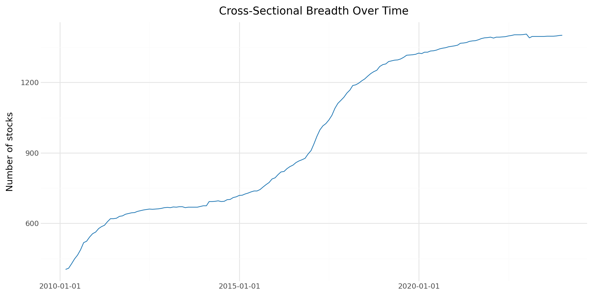
18.3.3 Loading Factor Data
We also load the Fama-French factor returns for risk-adjusted performance evaluation. These factors were constructed in previous chapters.
factors_ff3_monthly = pd.read_sql_query(
    sql="SELECT date, mkt_excess, smb, hml, risk_free FROM factors_ff3_monthly",
    con=tidy_finance,
    parse_dates={"date"}
)

print(f"Factor observations: {len(factors_ff3_monthly):,}")
print(f"Date range: {factors_ff3_monthly['date'].min().date()} "
      f"to {factors_ff3_monthly['date'].max().date()}")
Factor observations: 150
Date range: 2011-07-31 to 2023-12-3118.3.4 Data Quality Filters
Momentum strategies require continuous return histories for the formation period. We apply several filters to ensure data quality:
- Minimum price filter: We exclude penny stocks with prices below 1,000 VND, which are subject to extreme microstructure noise.
- Return availability: We require non-missing returns for the entire formation period.
- Market capitalization: We require positive lagged market capitalization for portfolio weighting.
# Filter for stocks with positive market cap and non-missing returns
prices_clean = (prices_monthly
    .dropna(subset=["ret", "mktcap"])
    .query("mktcap > 0")
    .sort_values(["symbol", "date"])
    .reset_index(drop=True)
)

print(f"Observations after filtering: {len(prices_clean):,}")
print(f"Stocks after filtering: {prices_clean['symbol'].nunique():,}")
Observations after filtering: 165,499
Stocks after filtering: 1,45718.4 Momentum Portfolio Construction
18.4.1 Computing Formation Period Returns
The first step in constructing momentum portfolios is to compute cumulative returns over the formation period. For a formation period of \(J\) months, we compute the cumulative return for each stock \(i\) at the end of month \(t\) as specified in Equation 35.7.
We implement this using a rolling product of gross returns. A key detail is that we require non-missing returns for all \(J\) months in the formation window. If any monthly return is missing, the cumulative return is set to missing, and the stock is excluded from portfolio formation in that month.
def compute_formation_returns(data, J):
    """
    Compute J-month cumulative returns for momentum portfolio formation.

    Parameters
    ----------
    data : pd.DataFrame
        Panel data with columns 'symbol', 'date', 'ret'.
    J : int
        Formation period length in months (typically 3-12).

    Returns
    -------
    pd.DataFrame
        Original data augmented with 'cum_return' column.
    """
    df = data.sort_values(["symbol", "date"]).copy()

    # Compute rolling J-month cumulative return
    # Using gross returns: (1+r1)*(1+r2)*...*(1+rJ) - 1
    df["gross_ret"] = 1 + df["ret"]

    df["cum_return"] = (
        df.groupby("symbol")["gross_ret"]
        .rolling(window=J, min_periods=J)
        .apply(np.prod, raw=True)
        .reset_index(level=0, drop=True)
        - 1
    )

    df = df.drop(columns=["gross_ret"])

    return df
Let us apply this function for our baseline case with \(J = 6\) months:
J = 6  # Formation period: 6 months

prices_with_cumret = compute_formation_returns(prices_clean, J)

# Check the result
print(f"Observations with valid {J}-month cumulative returns: "
      f"{prices_with_cumret['cum_return'].notna().sum():,}")
print(f"\nCumulative return distribution:")
print(prices_with_cumret["cum_return"].describe().round(4))
Observations with valid 6-month cumulative returns: 158,227
Cumulative return distribution:
count 158227.0000
mean 0.0171
std 0.5053
min -0.9999
25% -0.2196
50% -0.0400
75% 0.1404
max 35.7136
Name: cum_return, dtype: float6418.4.2 Assigning Momentum Decile Portfolios
Each month, we sort all stocks with valid cumulative returns into decile portfolios based on their past \(J\)-month performance. Portfolio 1 contains the bottom decile (losers) and portfolio 10 contains the top decile (winners).
def assign_momentum_portfolios(data, n_portfolios=10):
    """
    Assign stocks to momentum portfolios based on formation-period returns.

    For each cross-section (month), stocks are sorted into
    n_portfolios quantile groups according to their cumulative return.

    Portfolio 1 = lowest past returns (Losers)
    Portfolio n_portfolios = highest past returns (Winners)

    This implementation uses `groupby().transform()` rather than
    `groupby().apply()` to preserve the original DataFrame structure
    and avoid index mutation issues.

    Parameters
    ----------
    data : pd.DataFrame
        Panel data containing at minimum:
        - 'symbol' : stock identifier
        - 'date' : formation month
        - 'cum_return' : cumulative return over formation window

    n_portfolios : int, optional
        Number of portfolios to form (default = 10 for deciles).

    Returns
    -------
    pd.DataFrame
        Original data augmented with:
        - 'momr' : integer momentum rank (1 to n_portfolios)
    """

    # Drop observations without formation-period returns
    # These cannot be ranked into portfolios
    df = data.dropna(subset=["cum_return"]).copy()

    def safe_qcut(x):
        """
        Assign quantile portfolio labels within a single cross-section.

        Uses pd.qcut to create approximately equal-sized portfolios.
        If too few unique return values exist (which can happen in
        small markets or illiquid samples), fall back to rank-based
        binning to ensure portfolios are still formed.
        """
        try:
            # Standard quantile sorting
            return pd.qcut(
                x,
                q=n_portfolios,
                labels=range(1, n_portfolios + 1),
                duplicates="drop"  # prevents crash if quantile edges duplicate
            )
        except ValueError:
            # Fallback: rank then evenly cut into bins
            return pd.cut(
                x.rank(method="first"),
                bins=n_portfolios,
                labels=range(1, n_portfolios + 1)
            )

    # Cross-sectional portfolio assignment:
    # For each month, compute portfolio ranks based on cum_return.
    # transform ensures:
    # - original row order preserved
    # - no index mutation
    # - no loss of 'date' column
    df["momr"] = (
        df.groupby("date")["cum_return"]
          .transform(safe_qcut)
          .astype(int)
    )

    return df
portfolios = assign_momentum_portfolios(prices_with_cumret)
print(f"Stocks assigned to portfolios: {len(portfolios):,}")
print(f"\nPortfolio distribution (should be approximately equal):")
print(portfolios.groupby("momr")["symbol"].count().to_frame("count"))Stocks assigned to portfolios: 158,227
Portfolio distribution (should be approximately equal):
count
momr
1 15894
2 15815
3 16021
4 15759
5 15738
6 16568
7 15288
8 15582
9 15697
10 1586518.4.3 Defining Holding Period Dates
After forming portfolios at the end of month \(t\), we hold them from the beginning of month \(t+1\) through the end of month \(t+K\). This one-month gap between the formation period and the start of the holding period is standard in the literature and avoids the well-documented short-term reversal effect at the one-month horizon (Jegadeesh 1990).
K = 6  # Holding period: 6 months

portfolios_with_dates = portfolios.copy()
portfolios_with_dates = portfolios_with_dates.rename(
    columns={"date": "form_date"}
)

# Define holding period start and end dates
portfolios_with_dates["hdate1"] = (
    portfolios_with_dates["form_date"] + pd.offsets.MonthBegin(1)
)
portfolios_with_dates["hdate2"] = (
    portfolios_with_dates["form_date"] + pd.offsets.MonthEnd(K)
)

print(portfolios_with_dates[
    ["symbol", "form_date", "cum_return", "momr", "hdate1", "hdate2"]
].head(10))
symbol form_date cum_return momr hdate1 hdate2
5 A32 2019-04-30 -0.061599 4 2019-05-01 2019-10-31
6 A32 2019-05-31 -0.213675 2 2019-06-01 2019-11-30
7 A32 2019-06-30 -0.308720 2 2019-07-01 2019-12-31
8 A32 2019-07-31 -0.249936 2 2019-08-01 2020-01-31
9 A32 2019-08-31 0.061986 8 2019-09-01 2020-02-29
10 A32 2019-09-30 0.030751 8 2019-10-01 2020-03-31
11 A32 2019-10-31 0.030751 8 2019-11-01 2020-04-30
12 A32 2019-11-30 0.032486 8 2019-12-01 2020-05-31
13 A32 2019-12-31 0.180073 9 2020-01-01 2020-06-30
14 A32 2020-01-31 0.412322 10 2020-02-01 2020-07-3118.4.4 Computing Portfolio Holding Period Returns
We now compute the returns of each portfolio during its holding period. For each stock-formation date combination, we merge in the actual returns realized during the holding window. This produces a panel of stock returns indexed by formation date, holding date, and momentum portfolio rank.
# Merge: for each portfolio assignment, get all returns during holding period
portfolio_returns = portfolios_with_dates.merge(
    prices_clean[["symbol", "date", "ret"]].rename(
        columns={"ret": "hret", "date": "hdate"}
    ),
    on="symbol",
    how="inner"
)

# Keep only returns within the holding period
portfolio_returns = portfolio_returns.query(
    "hdate >= hdate1 and hdate <= hdate2"
)

print(f"Portfolio-holding period observations: {len(portfolio_returns):,}")
Portfolio-holding period observations: 918,07218.4.5 Computing Equally Weighted Portfolio Returns
The Jegadeesh and Titman (1993) methodology uses equally weighted portfolios. For each holding month, each momentum decile has \(K\) active cohorts (one formed in each of the past \(K\) months). We first compute the equally weighted return within each cohort, then average across cohorts to get the final monthly portfolio return.
# Step 1: Average return within each cohort (form_date × momr × hdate)
cohort_returns = (portfolio_returns
    .groupby(["hdate", "momr", "form_date"])
    .agg(cohort_ret=("hret", "mean"))
    .reset_index()
)

# Step 2: Average across cohorts for each momentum portfolio × month
ewret = (cohort_returns
    .groupby(["hdate", "momr"])
    .agg(
        ewret=("cohort_ret", "mean"),
        ewret_std=("cohort_ret", "std"),
        n_cohorts=("cohort_ret", "count")
    )
    .reset_index()
    .rename(columns={"hdate": "date"})
)

print(f"Monthly portfolio return observations: {len(ewret):,}")
print(f"Date range: {ewret['date'].min().date()} to {ewret['date'].max().date()}")
Monthly portfolio return observations: 1,610
Date range: 2010-08-31 to 2023-12-31We should verify that we have the expected number of active cohorts per month. Once the strategy has been running for at least \(K\) months, each momentum decile should have exactly \(K\) active cohorts.
cohort_check = (ewret
    .groupby("date")["n_cohorts"]
    .mean()
    .reset_index()
    .rename(columns={"n_cohorts": "avg_cohorts"})
)

plot_cohorts = (
    ggplot(cohort_check, aes(x="date", y="avg_cohorts")) +
    geom_line(color="#1f77b4") +
    geom_hline(yintercept=K, linetype="dashed", color="red") +
    labs(
        x="", y="Average number of cohorts",
        title=f"Active Cohorts per Portfolio (K={K})"
    ) +
    theme_minimal() +
    theme(figure_size=(10, 4))
)
plot_cohorts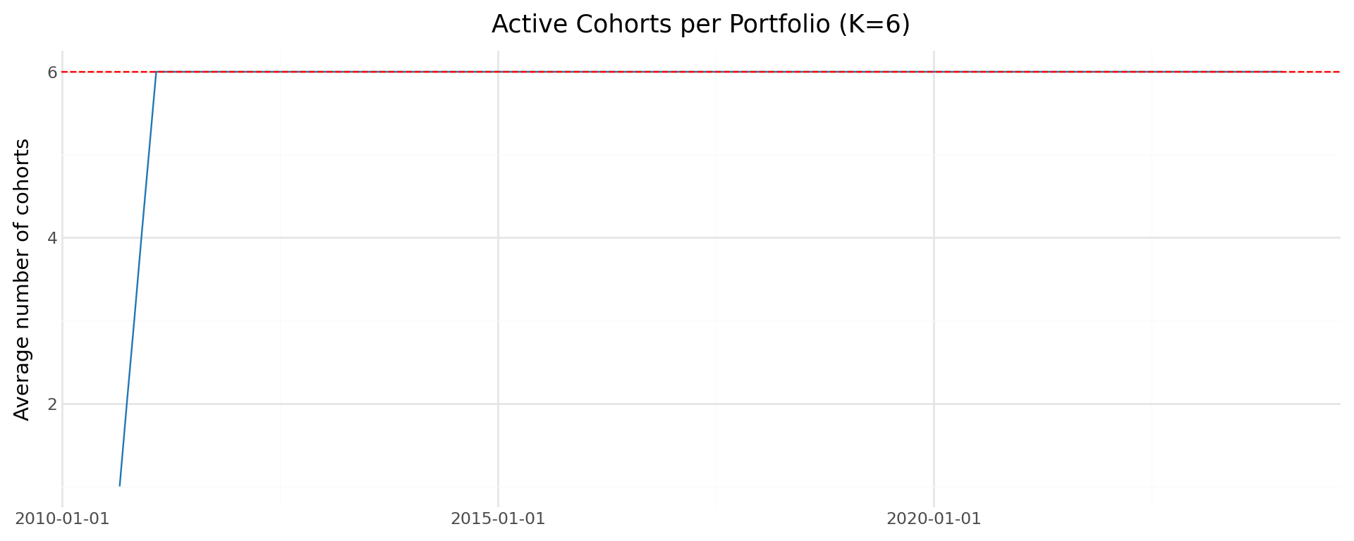
18.5 Baseline Results: J=6, K=6 Strategy
18.5.1 Summary Statistics by Momentum Decile
We now examine the average monthly returns for each momentum decile portfolio. Table 18.2 presents the mean, \(t\)-statistic, and \(p\)-value for each of the ten portfolios.
def compute_portfolio_stats(group):
    """Compute mean, t-stat, and p-value for a return series."""
    n = len(group)
    mean_ret = group.mean()
    std_ret = group.std()
    t_stat = mean_ret / (std_ret / np.sqrt(n)) if std_ret > 0 else np.nan
    p_val = 2 * (1 - stats.t.cdf(abs(t_stat), df=n-1)) if not np.isnan(t_stat) else np.nan
    return pd.Series({
        "N": n,
        "Mean (%)": mean_ret * 100,
        "Std (%)": std_ret * 100,
        "t-stat": t_stat,
        "p-value": p_val
    })

momentum_stats = (ewret
    .groupby("momr")["ewret"]
    .apply(compute_portfolio_stats)
    .unstack()
    .round(4)
)

momentum_stats| N | Mean (%) | Std (%) | t-stat | p-value | |
|---|---|---|---|---|---|
| momr | |||||
| 1 | 161.0 | 1.4190 | 6.5319 | 2.7565 | 0.0065 |
| 2 | 161.0 | 0.6602 | 5.9895 | 1.3985 | 0.1639 |
| 3 | 161.0 | 0.3658 | 5.5080 | 0.8427 | 0.4007 |
| 4 | 161.0 | 0.1623 | 5.0085 | 0.4112 | 0.6815 |
| 5 | 161.0 | 0.0111 | 4.7561 | 0.0297 | 0.9763 |
| 6 | 161.0 | 0.0408 | 4.6864 | 0.1104 | 0.9122 |
| 7 | 161.0 | -0.0674 | 4.8881 | -0.1749 | 0.8614 |
| 8 | 161.0 | -0.2066 | 4.9208 | -0.5329 | 0.5949 |
| 9 | 161.0 | -0.2228 | 5.3013 | -0.5332 | 0.5946 |
| 10 | 161.0 | -0.6812 | 5.7131 | -1.5130 | 0.1323 |
18.5.2 The Long-Short Momentum Portfolio
The key test of the momentum effect is whether the spread between winners and losers—the long-short momentum portfolio—generates statistically significant positive returns. We construct this spread portfolio by going long the top decile (portfolio 10) and short the bottom decile (portfolio 1).
# Pivot to wide format
ewret_wide = ewret.pivot(
    index="date", columns="momr", values="ewret"
).reset_index()

ewret_wide.columns = ["date"] + [f"port{i}" for i in range(1, 11)]

# Compute long-short return
ewret_wide["winners"] = ewret_wide["port10"]
ewret_wide["losers"] = ewret_wide["port1"]
ewret_wide["long_short"] = ewret_wide["winners"] - ewret_wide["losers"]
ls_stats = pd.DataFrame()
for col in ["winners", "losers", "long_short"]:
series = ewret_wide[col].dropna()
n = len(series)
mean_val = series.mean()
std_val = series.std()
t_val = mean_val / (std_val / np.sqrt(n))
p_val = 2 * (1 - stats.t.cdf(abs(t_val), df=n-1))
ls_stats[col] = [n, mean_val * 100, std_val * 100, t_val, p_val]
ls_stats.index = ["N", "Mean (%)", "Std (%)", "t-stat", "p-value"]
ls_stats.columns = ["Winners", "Losers", "Long-Short"]
ls_stats = ls_stats.round(4)
ls_stats| Winners | Losers | Long-Short | |
|---|---|---|---|
| N | 161.0000 | 161.0000 | 161.0000 |
| Mean (%) | -0.6812 | 1.4190 | -2.1002 |
| Std (%) | 5.7131 | 6.5319 | 4.8969 |
| t-stat | -1.5130 | 2.7565 | -5.4420 |
| p-value | 0.1323 | 0.0065 | 0.0000 |
18.5.3 Cumulative Returns
The time-series evolution of cumulative returns provides visual evidence of the momentum strategy’s performance. Figure 18.3 shows the cumulative returns of the winner and loser portfolios, while Figure 18.4 shows the cumulative return of the long-short momentum strategy.
# Compute cumulative returns
ewret_wide = ewret_wide.sort_values("date").reset_index(drop=True)

for col in ["winners", "losers", "long_short"]:
    ewret_wide[f"cumret_{col}"] = (1 + ewret_wide[col]).cumprod() - 1
cumret_plot_data = (ewret_wide
[["date", "cumret_winners", "cumret_losers"]]
.melt(id_vars="date", var_name="portfolio", value_name="cumret")
)
cumret_plot_data["portfolio"] = cumret_plot_data["portfolio"].map({
"cumret_winners": "Winners (P10)",
"cumret_losers": "Losers (P1)"
})
plot_cumret = (
ggplot(cumret_plot_data,
aes(x="date", y="cumret", color="portfolio")) +
geom_line(size=1) +
scale_y_continuous(labels=percent_format()) +
scale_color_manual(values=["#d62728", "#1f77b4"]) +
labs(
x="", y="Cumulative return",
color="Portfolio",
title="Cumulative Returns: Winners vs. Losers"
) +
theme_minimal() +
theme(
figure_size=(10, 6),
legend_position="bottom"
)
)
plot_cumret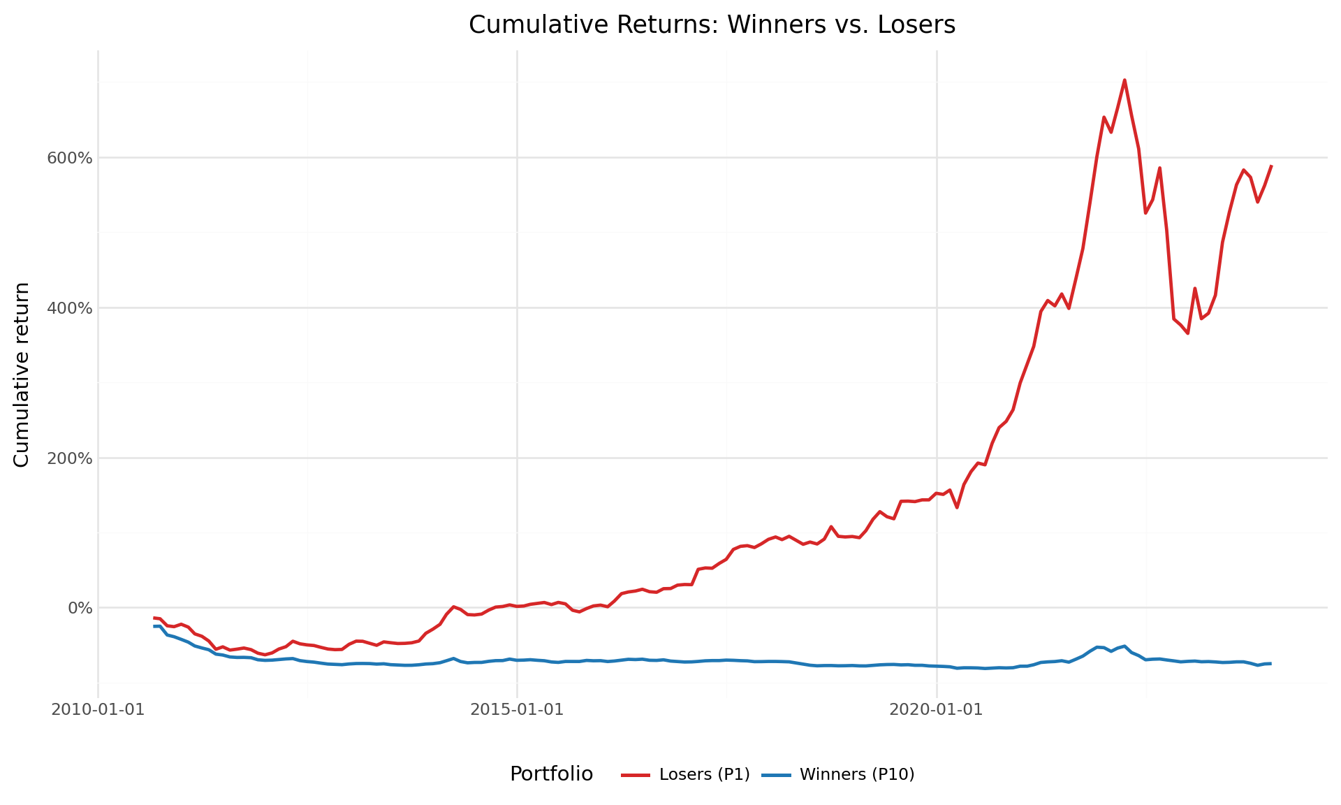
plot_ls = (
    ggplot(ewret_wide, aes(x="date", y="cumret_long_short")) +
    geom_line(size=1, color="#2ca02c") +
    geom_hline(yintercept=0, linetype="dashed", color="gray") +
    scale_y_continuous(labels=percent_format()) +
    labs(
        x="", y="Cumulative return",
        title="Cumulative Return: Long-Short Momentum Strategy"
    ) +
    theme_minimal() +
    theme(figure_size=(10, 6))
)
plot_ls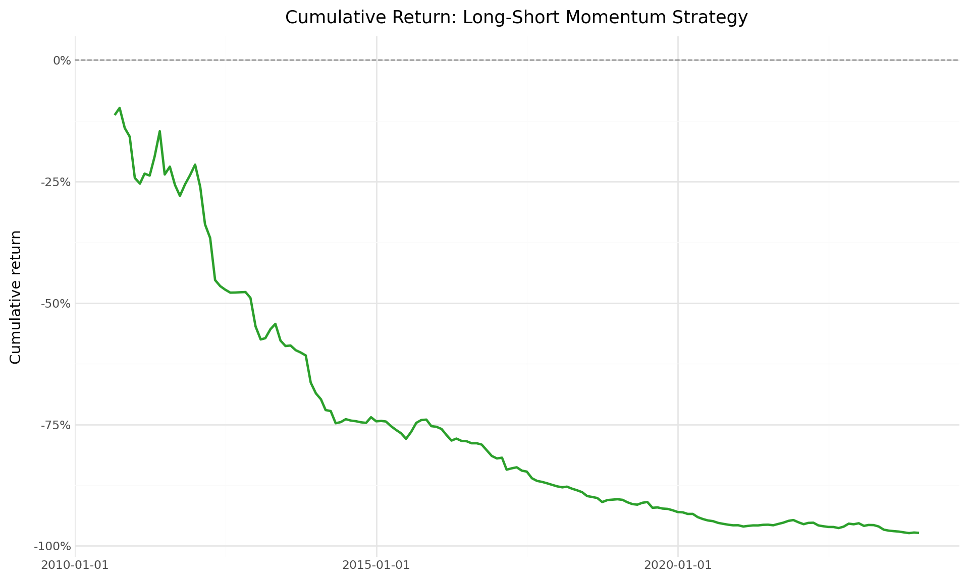
18.5.4 Monthly Return Distribution
Beyond the mean, the full distribution of monthly long-short returns provides insight into the risk profile of the momentum strategy. Figure 39.1 shows the histogram of monthly returns.
mean_ls = ewret_wide["long_short"].mean()

plot_dist = (
    ggplot(ewret_wide, aes(x="long_short")) +
    geom_histogram(bins=50, fill="#1f77b4", alpha=0.7) +
    geom_vline(xintercept=mean_ls, linetype="dashed", color="red") +
    scale_x_continuous(labels=percent_format()) +
    labs(
        x="Monthly long-short return",
        y="Frequency",
        title="Distribution of Monthly Momentum Returns"
    ) +
    theme_minimal() +
    theme(figure_size=(10, 5))
)
plot_dist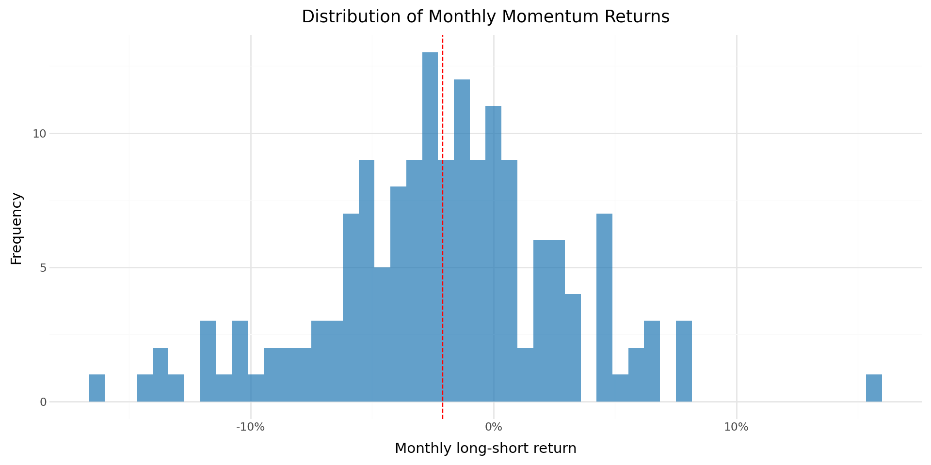
18.6 Extending to Multiple Formation and Holding Periods
18.6.1 The J × K Grid
Jegadeesh and Titman (1993) evaluate momentum strategies across a comprehensive grid of formation periods \(J \in \{3, 6, 9, 12\}\) and holding periods \(K \in \{3, 6, 9, 12\}\). This produces 16 different strategy specifications, allowing us to assess the robustness of the momentum effect across different horizons.
We now implement a function that computes the full momentum strategy for any given \((J, K)\) pair, wrapping the steps developed above into a single reusable pipeline.
from joblib import Parallel, delayed
import time

def momentum_strategy(data, J, K, n_portfolios=10):
    """
    Implement the full Jegadeesh-Titman momentum strategy.

    Parameters
    ----------
    data : pd.DataFrame
        Panel of stock returns with columns: symbol, date, ret.
    J : int
        Formation period in months.
    K : int
        Holding period in months.
    n_portfolios : int
        Number of portfolios (default: 10 for deciles).

    Returns
    -------
    pd.DataFrame
        Monthly returns for each momentum portfolio and the long-short spread.
    """
    # Step 1: Compute formation period cumulative returns
    df = data.sort_values(["symbol", "date"]).copy()
    df["gross_ret"] = 1 + df["ret"]
    df["cum_return"] = (
        df.groupby("symbol")["gross_ret"]
        .rolling(window=J, min_periods=J)
        .apply(np.prod, raw=True)
        .reset_index(level=0, drop=True)
        - 1
    )
    df = df.drop(columns=["gross_ret"]).dropna(subset=["cum_return"])

    # Step 2: Assign to momentum portfolios using transform
    df["momr"] = df.groupby("date", observed=True)["cum_return"].transform(
        lambda x: pd.qcut(
            x,
            q=n_portfolios,
            labels=range(1, n_portfolios + 1),
            duplicates="drop"
        )
    ).astype('Int64')

    # If any NaNs in momr, fill with rank-based assignment
    mask = df["momr"].isna()
    if mask.any():
        df.loc[mask, "momr"] = df.loc[mask].groupby("date")["cum_return"].transform(
            lambda x: pd.qcut(
                x.rank(method="first"),
                q=min(n_portfolios, len(x.unique())),
                labels=False,
                duplicates="drop"
            )
        ).astype('Int64') + 1

    # Step 3: Define holding period dates
    df = df.rename(columns={"date": "form_date"})
    df["hdate1"] = df["form_date"] + pd.offsets.MonthBegin(1)
    df["hdate2"] = df["form_date"] + pd.offsets.MonthEnd(K)

    # Step 4: Merge with holding period returns
    port_ret = df[["symbol", "form_date", "momr", "hdate1", "hdate2"]].merge(
        data[["symbol", "date", "ret"]].rename(
            columns={"ret": "hret", "date": "hdate"}
        ),
        on="symbol",
        how="inner"
    )

    # Use boolean indexing
    port_ret = port_ret[
        (port_ret["hdate"] >= port_ret["hdate1"]) &
        (port_ret["hdate"] <= port_ret["hdate2"])
    ]

    # Step 5: Compute equally weighted returns (two-stage averaging)
    cohort_ret = (port_ret
        .groupby(["hdate", "momr", "form_date"])
        .agg(cohort_ret=("hret", "mean"))
        .reset_index()
    )

    monthly_ret = (cohort_ret
        .groupby(["hdate", "momr"])
        .agg(ewret=("cohort_ret", "mean"))
        .reset_index()
        .rename(columns={"hdate": "date"})
    )

    # Step 6: Compute long-short spread
    wide = monthly_ret.pivot(
        index="date", columns="momr", values="ewret"
    ).reset_index()

    # Handle variable number of portfolios
    n_cols = len(wide.columns) - 1
    wide.columns = ["date"] + [f"port{i}" for i in range(1, n_cols + 1)]
    wide["winners"] = wide[f"port{n_cols}"]
    wide["losers"] = wide["port1"]
    wide["long_short"] = wide["winners"] - wide["losers"]

    return monthly_ret, wide
18.6.2 Running the Full Grid
We now run the momentum strategy for all 16 \((J, K)\) combinations. This is computationally intensive, so we store the key summary statistics for each specification.
18.6.2.1 Sequential Calculation
J_values = [3, 6, 9, 12]
K_values = [3, 6, 9, 12]

results_grid = []

for J_val, K_val in product(J_values, K_values):
    print(f"Computing J={J_val}, K={K_val}...", end=" ")

    try:
        _, wide_result = momentum_strategy(prices_clean, J_val, K_val)

        for portfolio_name in ["winners", "losers", "long_short"]:
            series = wide_result[portfolio_name].dropna()
            n = len(series)
            mean_ret = series.mean()
            std_ret = series.std()
            t_stat = mean_ret / (std_ret / np.sqrt(n)) if std_ret > 0 else np.nan
            p_val = (2 * (1 - stats.t.cdf(abs(t_stat), df=n-1))
                     if not np.isnan(t_stat) else np.nan)

            results_grid.append({
                "J": J_val,
                "K": K_val,
                "portfolio": portfolio_name,
                "n_months": n,
                "mean_ret": mean_ret,
                "std_ret": std_ret,
                "t_stat": t_stat,
                "p_value": p_val
            })

        print("Done.")
    except Exception as e:
        print(f"Error: {e}")

results_df = pd.DataFrame(results_grid)
18.6.2.2 Parallel Calculation
def compute_single_strategy(data, J, K):
    """
    Compute statistics for a single (J, K) strategy.
    Returns a list of result dicts, one per portfolio.
    """
    try:
        _, wide_result = momentum_strategy(data, J, K)

        results = []
        for portfolio_name in ["winners", "losers", "long_short"]:
            series = wide_result[portfolio_name].dropna()
            n = len(series)
            mean_ret = series.mean()
            std_ret = series.std()
            t_stat = mean_ret / (std_ret / np.sqrt(n)) if std_ret > 0 else np.nan
            p_val = (2 * (1 - stats.t.cdf(abs(t_stat), df=n-1))
                     if not np.isnan(t_stat) else np.nan)

            results.append({
                "J": J,
                "K": K,
                "portfolio": portfolio_name,
                "n_months": n,
                "mean_ret": mean_ret,
                "std_ret": std_ret,
                "t_stat": t_stat,
                "p_value": p_val
            })
        return results
    except Exception as e:
        print(f"Error in J={J}, K={K}: {e}")
        return []
J_values = [3, 6, 9, 12]
K_values = [3, 6, 9, 12]
# Create list of (J, K) pairs
params = list(product(J_values, K_values))
print(f"Running {len(params)} momentum strategies in parallel with 4 cores...")
start_time = time.time()
# Parallel execution with 4 workers
results_list = Parallel(n_jobs=4, verbose=10)(
delayed(compute_single_strategy)(prices_clean, J, K)
for J, K in params
)
# Flatten results
results_grid = [item for sublist in results_list for item in sublist]
results_df = pd.DataFrame(results_grid)
elapsed = time.time() - start_time
print(f"\nCompleted in {elapsed:.2f} seconds")Running 16 momentum strategies in parallel with 4 cores...[Parallel(n_jobs=4)]: Using backend LokyBackend with 4 concurrent workers.
[Parallel(n_jobs=4)]: Done 5 tasks | elapsed: 8.4s
[Parallel(n_jobs=4)]: Done 11 out of 16 | elapsed: 14.4s remaining: 6.5s
[Parallel(n_jobs=4)]: Done 13 out of 16 | elapsed: 18.7s remaining: 4.3s
Completed in 19.68 seconds[Parallel(n_jobs=4)]: Done 16 out of 16 | elapsed: 19.6s finished# Summary statistics
print("\nResults Summary by Formation Period:")
print(results_df.groupby("J").agg({
"mean_ret": "mean",
"std_ret": "mean",
"t_stat": ["mean", lambda x: (x.abs() > 1.96).sum()],
"n_months": "first"
}).round(6))
Results Summary by Formation Period:
    mean_ret   std_ret    t_stat            n_months
        mean      mean      mean <lambda_0>    first
J
6  -0.004661  0.055672 -1.517507          9      161
9  -0.003265  0.056520 -1.071904          9      158
12 -0.002759  0.058194 -0.931273          9      155
18.6.3 Winners Portfolio Returns
Table 18.4 presents the average monthly returns of the winner portfolio (portfolio 10) across all \((J, K)\) combinations.
winners_grid = (results_df
    .query("portfolio == 'winners'")
    .assign(
        display=lambda x: (
            x["mean_ret"].apply(lambda v: f"{v*100:.2f}") +
            "\n(" + x["t_stat"].apply(lambda v: f"{v:.2f}") + ")"
        )
    )
    .pivot(index="J", columns="K", values="display")
)
winners_grid.columns = [f"K={k}" for k in winners_grid.columns]
winners_grid.index = [f"J={j}" for j in winners_grid.index]
winners_grid| K=3 | K=6 | K=9 | K=12 | |
|---|---|---|---|---|
| J=6 | -1.18\n(-2.65) | -0.68\n(-1.51) | -0.55\n(-1.23) | -0.39\n(-0.87) |
| J=9 | -1.00\n(-2.36) | -0.51\n(-1.22) | -0.28\n(-0.68) | -0.16\n(-0.39) |
| J=12 | -0.88\n(-2.09) | -0.39\n(-0.91) | -0.24\n(-0.56) | -0.14\n(-0.34) |
18.6.4 Losers Portfolio Returns
Table 18.5 presents the corresponding results for the loser portfolio.
losers_grid = (results_df
    .query("portfolio == 'losers'")
    .assign(
        display=lambda x: (
            x["mean_ret"].apply(lambda v: f"{v*100:.2f}") +
            "\n(" + x["t_stat"].apply(lambda v: f"{v:.2f}") + ")"
        )
    )
    .pivot(index="J", columns="K", values="display")
)
losers_grid.columns = [f"K={k}" for k in losers_grid.columns]
losers_grid.index = [f"J={j}" for j in losers_grid.index]
losers_grid| K=3 | K=6 | K=9 | K=12 | |
|---|---|---|---|---|
| J=6 | 1.87\n(3.49) | 1.42\n(2.76) | 1.10\n(2.19) | 0.99\n(1.99) |
| J=9 | 1.94\n(3.51) | 1.38\n(2.56) | 1.21\n(2.31) | 1.15\n(2.22) |
| J=12 | 1.57\n(2.71) | 1.29\n(2.28) | 1.19\n(2.13) | 1.15\n(2.09) |
18.6.5 Long-Short Momentum Returns
Table 18.6 presents the most important results: the average monthly returns of the long-short momentum portfolio across all specifications.
ls_grid = (results_df
    .query("portfolio == 'long_short'")
    .assign(
        display=lambda x: (
            x["mean_ret"].apply(lambda v: f"{v*100:.2f}") +
            "\n(" + x["t_stat"].apply(lambda v: f"{v:.2f}") + ")"
        )
    )
    .pivot(index="J", columns="K", values="display")
)
ls_grid.columns = [f"K={k}" for k in ls_grid.columns]
ls_grid.index = [f"J={j}" for j in ls_grid.index]
ls_grid| K=3 | K=6 | K=9 | K=12 | |
|---|---|---|---|---|
| J=6 | -3.04\n(-7.38) | -2.10\n(-5.44) | -1.65\n(-4.94) | -1.37\n(-4.61) |
| J=9 | -2.94\n(-6.41) | -1.89\n(-4.55) | -1.49\n(-3.98) | -1.31\n(-3.87) |
| J=12 | -2.45\n(-5.42) | -1.68\n(-3.92) | -1.43\n(-3.60) | -1.30\n(-3.55) |
18.6.6 Visualizing the Momentum Premium Across Specifications
Figure 18.6 provides a visual summary of the long-short momentum premium across all \((J, K)\) combinations.
ls_heatmap_data = (results_df
    .query("portfolio == 'long_short'")
    .assign(
        mean_pct=lambda x: x["mean_ret"] * 100,
        significant=lambda x: x["p_value"] < 0.05,
        label=lambda x: x.apply(
            lambda row: f"{row['mean_ret']*100:.2f}{'*' if row['p_value'] < 0.05 else ''}",
            axis=1
        )
    )
)

plot_heatmap = (
    ggplot(ls_heatmap_data,
           aes(x="K.astype(str)", y="J.astype(str)", fill="mean_pct")) +
    geom_tile(color="white", size=2) +
    geom_text(aes(label="label"), size=10, color="white") +
    scale_fill_gradient2(
        low="#d62728", mid="#f7f7f7", high="#1f77b4", midpoint=0,
        name="Monthly\nReturn (%)"
    ) +
    labs(
        x="Holding Period (K months)",
        y="Formation Period (J months)",
        title="Momentum Premium Across J×K Specifications"
    ) +
    theme_minimal() +
    theme(figure_size=(8, 6))
)
plot_heatmap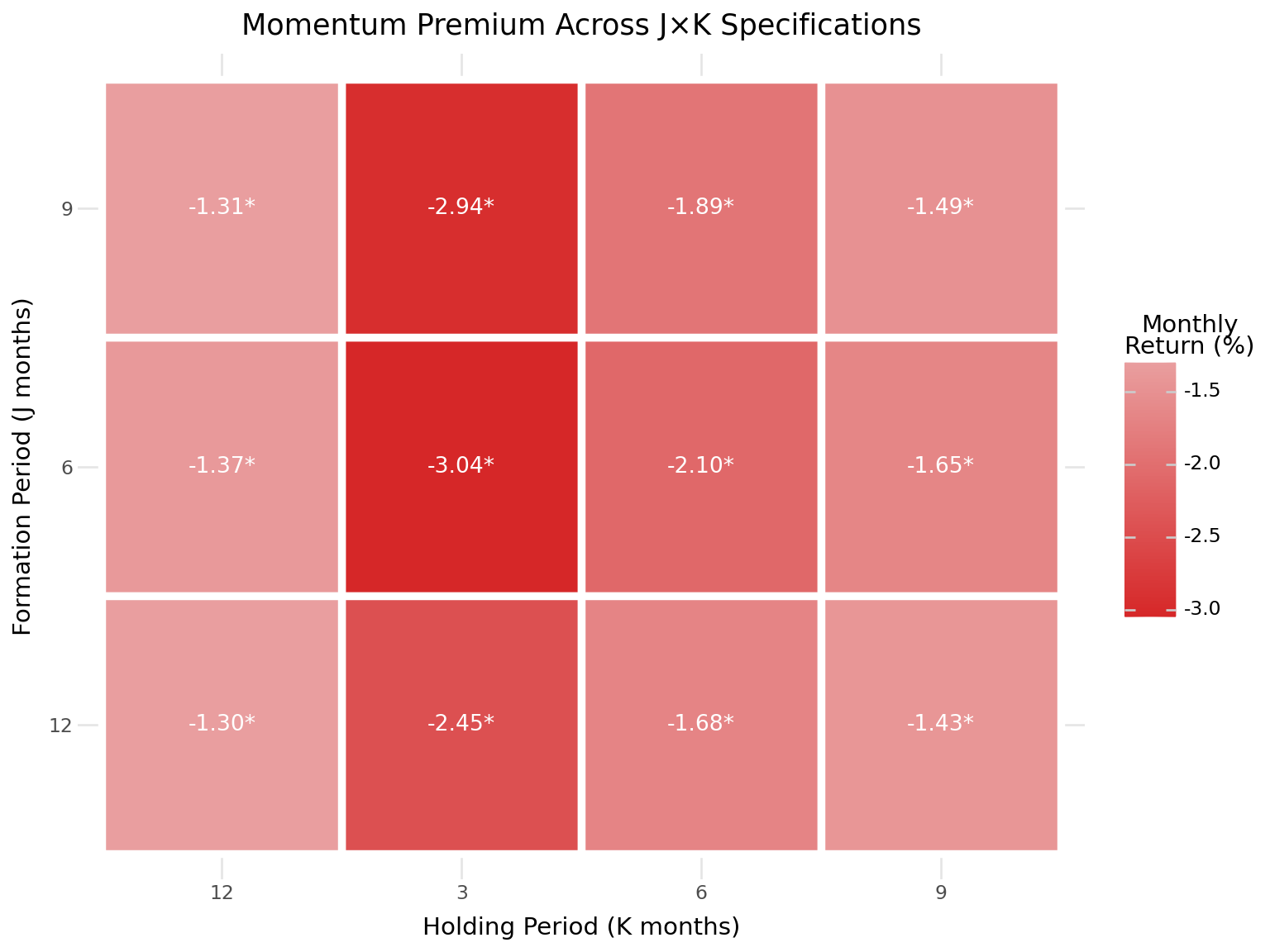
18.7 Risk-Adjusted Performance
18.7.1 CAPM Alpha
A natural question is whether the momentum premium is explained by exposure to the market factor. We estimate the CAPM alpha of the long-short momentum portfolio by regressing its returns on the market excess return:
\[ r_{\text{WML},t} = \alpha + \beta \cdot r_{\text{MKT},t} + \epsilon_t \tag{18.3}\]
# Merge momentum returns with factor data (baseline J=6, K=6)
ewret_factors = (ewret_wide
    [["date", "winners", "losers", "long_short"]]
    .merge(factors_ff3_monthly, on="date", how="inner")
)

# CAPM regression for long-short portfolio
from statsmodels.formula.api import ols as ols_formula
import statsmodels.api as sm

X_capm = sm.add_constant(ewret_factors["mkt_excess"])
y_ls = ewret_factors["long_short"]

capm_model = sm.OLS(y_ls, X_capm).fit(cov_type="HAC", cov_kwds={"maxlags": 6})

print("CAPM Regression: Long-Short Momentum Returns")
print("=" * 60)
print(f"Alpha (monthly):  {capm_model.params['const']*100:.4f}% "
      f"(t={capm_model.tvalues['const']:.2f})")
print(f"Market Beta:      {capm_model.params['mkt_excess']:.4f} "
      f"(t={capm_model.tvalues['mkt_excess']:.2f})")
print(f"R-squared:        {capm_model.rsquared:.4f}")
print(f"N observations:   {capm_model.nobs:.0f}")
CAPM Regression: Long-Short Momentum Returns
============================================================
Alpha (monthly): -2.2703% (t=-5.05)
Market Beta: -0.1779 (t=-1.75)
R-squared: 0.0470
N observations: 15018.7.2 Fama-French Three-Factor Alpha
We extend the risk adjustment to the Fama-French three-factor model, which includes the size (SMB) and value (HML) factors in addition to the market factor:
\[ r_{\text{WML},t} = \alpha + \beta_1 \cdot r_{\text{MKT},t} + \beta_2 \cdot \text{SMB}_t + \beta_3 \cdot \text{HML}_t + \epsilon_t \tag{18.4}\]
X_ff3 = sm.add_constant(
    ewret_factors[["mkt_excess", "smb", "hml"]]
)
y_ls = ewret_factors["long_short"]

ff3_model = sm.OLS(y_ls, X_ff3).fit(cov_type="HAC", cov_kwds={"maxlags": 6})

# Display results as a clean table
ff3_results = pd.DataFrame({
    "Coefficient": ff3_model.params,
    "Std Error": ff3_model.bse,
    "t-stat": ff3_model.tvalues,
    "p-value": ff3_model.pvalues
}).round(4)

ff3_results.index = ["Alpha", "MKT", "SMB", "HML"]
ff3_results| Coefficient | Std Error | t-stat | p-value | |
|---|---|---|---|---|
| Alpha | -0.0234 | 0.0041 | -5.7189 | 0.0000 |
| MKT | -0.1269 | 0.1558 | -0.8145 | 0.4154 |
| SMB | 0.1123 | 0.1882 | 0.5969 | 0.5506 |
| HML | 0.0716 | 0.1414 | 0.5065 | 0.6125 |
print(f"\nR-squared: {ff3_model.rsquared:.4f}")
print(f"Adjusted R-squared: {ff3_model.rsquared_adj:.4f}")
print(f"Alpha (annualized): {ff3_model.params['const'] * 12 * 100:.2f}%")
R-squared: 0.0553
Adjusted R-squared: 0.0359
Alpha (annualized): -28.02%
18.7.3 Interpretation of Risk Exposures
The factor loadings from the three-factor regression reveal the risk characteristics of the momentum strategy in the Vietnamese market. Several patterns are commonly observed:
Market beta: Momentum portfolios typically have moderate market exposure. In the U.S., Grundy and Martin (2001) document that the market beta of the long-short portfolio is close to zero on average but highly time-varying, spiking during market reversals.
Size exposure (SMB): Momentum strategies often load positively on the size factor, reflecting the tendency for smaller stocks to exhibit stronger momentum patterns.
Value exposure (HML): The long-short momentum portfolio typically loads negatively on HML, indicating that winners tend to be growth stocks while losers tend to be value stocks. This creates a natural tension between momentum and value strategies.
18.8 Momentum and Market States
18.8.1 Conditional Performance
An important finding in the momentum literature is that momentum profits vary with market conditions. Cooper, Gutierrez Jr, and Hameed (2004) document that momentum strategies perform well following market gains (UP markets) but experience severe losses following market declines (DOWN markets). This asymmetry is particularly relevant for emerging markets, which experience more extreme market states.
We define market states based on the cumulative market return over the prior 12 months:
\[ \text{Market State}_t = \begin{cases} \text{UP} & \text{if } \prod_{s=t-12}^{t-1}(1 + r_{m,s}) - 1 > 0 \\ \text{DOWN} & \text{otherwise} \end{cases} \tag{18.5}\]
# Compute 12-month lagged market return
market_returns = factors_ff3_monthly[["date", "mkt_excess"]].copy()
market_returns = market_returns.sort_values("date")
market_returns["mkt_cum_12m"] = (
    (1 + market_returns["mkt_excess"])
    .rolling(window=12, min_periods=12)
    .apply(np.prod, raw=True)
    - 1
)
market_returns["market_state"] = np.where(
    market_returns["mkt_cum_12m"] > 0, "UP", "DOWN"
)

# Merge with momentum returns
ewret_states = ewret_wide[["date", "long_short"]].merge(
    market_returns[["date", "market_state"]], on="date", how="inner"
).dropna()
state_stats = []
for state in ["UP", "DOWN"]:
subset = ewret_states.query(f"market_state == '{state}'")["long_short"]
n = len(subset)
mean_ret = subset.mean()
std_ret = subset.std()
t_stat = mean_ret / (std_ret / np.sqrt(n)) if std_ret > 0 else np.nan
p_val = 2 * (1 - stats.t.cdf(abs(t_stat), df=n-1)) if not np.isnan(t_stat) else np.nan
state_stats.append({
"Market State": state,
"N Months": n,
"Mean (%)": mean_ret * 100,
"Std (%)": std_ret * 100,
"t-stat": t_stat,
"p-value": p_val
})
state_stats_df = pd.DataFrame(state_stats).round(4)
state_stats_df| Market State | N Months | Mean (%) | Std (%) | t-stat | p-value | |
|---|---|---|---|---|---|---|
| 0 | UP | 39 | -1.1972 | 4.5814 | -1.6320 | 0.1109 |
| 1 | DOWN | 111 | -2.4050 | 4.8669 | -5.2063 | 0.0000 |
plot_states = (
    ggplot(ewret_states, aes(x="market_state", y="long_short",
                              fill="market_state")) +
    geom_boxplot(alpha=0.7) +
    geom_hline(yintercept=0, linetype="dashed", color="gray") +
    scale_y_continuous(labels=percent_format()) +
    scale_fill_manual(values={"UP": "#1f77b4", "DOWN": "#d62728"}) +
    labs(
        x="Market State (Prior 12-Month Return)",
        y="Monthly Long-Short Return",
        title="Momentum Returns by Market State"
    ) +
    theme_minimal() +
    theme(
        figure_size=(8, 6),
        legend_position="none"
    )
)
plot_states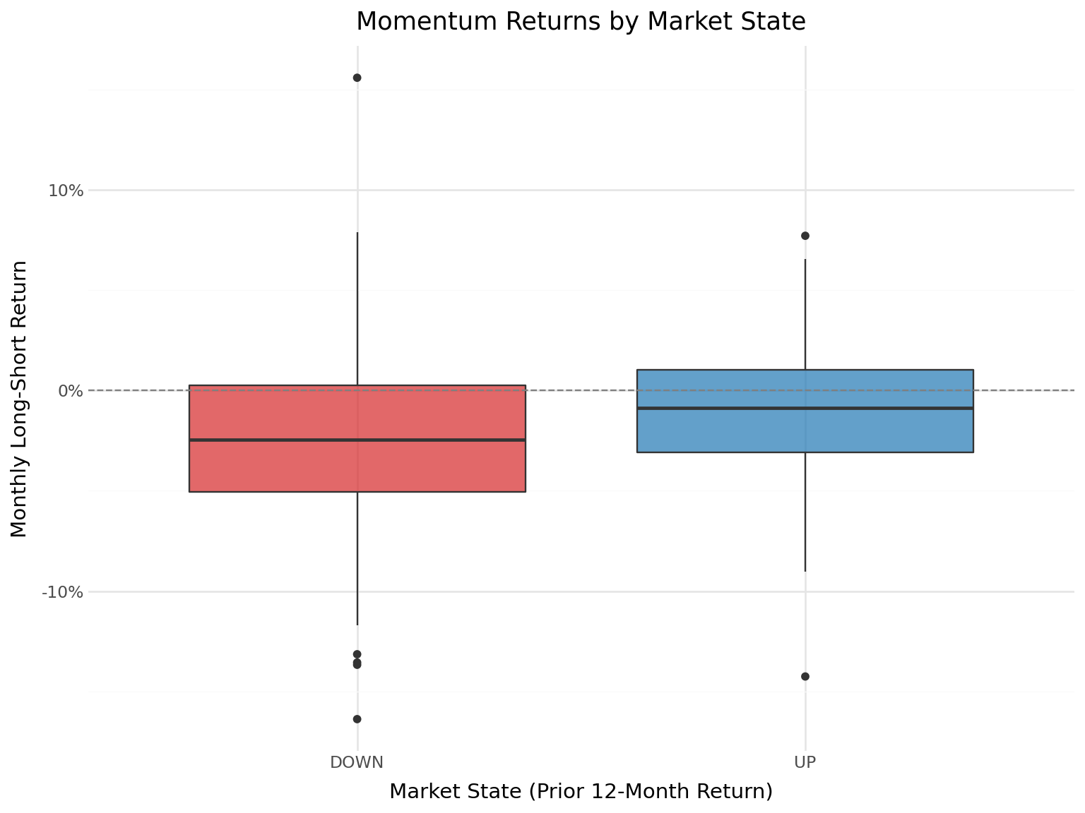
18.9 Momentum Crashes
18.9.1 Understanding Momentum Drawdowns
One of the most important risk characteristics of momentum strategies is their susceptibility to sudden, severe losses—known as momentum crashes. Daniel and Moskowitz (2016) document that momentum strategies experience infrequent but extreme losses, typically during market rebounds following bear markets. These crashes occur because the loser portfolio, which has been short, is heavily loaded with high-beta stocks that surge when markets reverse.
We identify the worst drawdowns of the momentum strategy and examine their market context.
worst_months = (ewret_wide
    [["date", "long_short", "winners", "losers"]]
    .merge(factors_ff3_monthly[["date", "mkt_excess"]], on="date", how="left")
    .sort_values("long_short")
    .head(10)
    .assign(
        long_short_pct=lambda x: (x["long_short"] * 100).round(2),
        winners_pct=lambda x: (x["winners"] * 100).round(2),
        losers_pct=lambda x: (x["losers"] * 100).round(2),
        mkt_pct=lambda x: (x["mkt_excess"] * 100).round(2)
    )
    [["date", "long_short_pct", "winners_pct", "losers_pct", "mkt_pct"]]
    .rename(columns={
        "date": "Date",
        "long_short_pct": "L/S (%)",
        "winners_pct": "Winners (%)",
        "losers_pct": "Losers (%)",
        "mkt_pct": "Market (%)"
    })
)
worst_months| Date | L/S (%) | Winners (%) | Losers (%) | Market (%) | |
|---|---|---|---|---|---|
| 153 | 2023-05-31 | -16.39 | -2.69 | 13.70 | 2.78 |
| 39 | 2013-11-30 | -14.26 | 4.24 | 18.50 | 2.57 |
| 20 | 2012-04-30 | -13.68 | 1.51 | 15.19 | 4.88 |
| 78 | 2017-02-28 | -13.56 | 2.10 | 15.67 | 1.49 |
| 107 | 2019-07-31 | -13.15 | -2.46 | 10.69 | 1.61 |
| 140 | 2022-04-30 | -11.71 | -17.57 | -5.87 | -11.19 |
| 149 | 2023-01-31 | -11.53 | 1.37 | 12.90 | 6.96 |
| 28 | 2012-12-31 | -11.52 | 4.03 | 15.54 | -1.61 |
| 0 | 2010-08-31 | -11.31 | -25.03 | -13.72 | NaN |
| 10 | 2011-06-30 | -10.44 | -3.15 | 7.29 | NaN |
18.9.2 Maximum Drawdown Analysis
The maximum drawdown provides a measure of the worst peak-to-trough decline experienced by the strategy. This metric is particularly relevant for practitioners evaluating the risk of momentum strategies.
# Compute running maximum and drawdown
ewret_wide["cum_wealth"] = (1 + ewret_wide["long_short"]).cumprod()
ewret_wide["running_max"] = ewret_wide["cum_wealth"].cummax()
ewret_wide["drawdown"] = (
    ewret_wide["cum_wealth"] / ewret_wide["running_max"] - 1
)

max_dd = ewret_wide["drawdown"].min()
max_dd_date = ewret_wide.loc[ewret_wide["drawdown"].idxmin(), "date"]

print(f"Maximum drawdown: {max_dd*100:.2f}%")
print(f"Date of maximum drawdown: {max_dd_date.date()}")
Maximum drawdown: -97.08%
Date of maximum drawdown: 2023-10-31plot_dd = (
ggplot(ewret_wide, aes(x="date", y="drawdown")) +
geom_area(fill="#d62728", alpha=0.5) +
geom_line(color="#d62728", size=0.5) +
scale_y_continuous(labels=percent_format()) +
labs(
x="", y="Drawdown",
title="Momentum Strategy Drawdown"
) +
theme_minimal() +
theme(figure_size=(10, 5))
)
plot_dd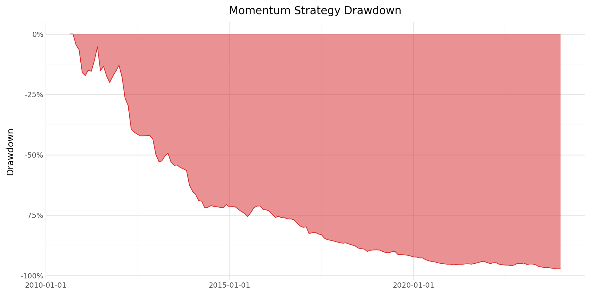
18.10 Value-Weighted Momentum Portfolios
The baseline Jegadeesh and Titman (1993) implementation uses equally weighted portfolios. However, equally weighted returns can be dominated by small, illiquid stocks that may be difficult to trade in practice. Value-weighted portfolios, where each stock’s contribution is proportional to its market capitalization, provide a more investable benchmark and are more representative of the returns that large investors could actually achieve.
def momentum_strategy_vw(data, J, K, n_portfolios=10):
    """
    Value-weighted momentum strategy implementation.

    Same as the equally-weighted version but uses lagged market
    capitalization as weights when computing portfolio returns.

    Parameters
    ----------
    data : pd.DataFrame
        Panel with columns: symbol, date, ret, mktcap_lag.
    J : int
        Formation period in months.
    K : int
        Holding period in months.
    n_portfolios : int
        Number of portfolios.

    Returns
    -------
    pd.DataFrame
        Monthly value-weighted portfolio returns.
    """
    # Step 1: Formation period returns
    df = data.sort_values(["symbol", "date"]).copy()
    df["gross_ret"] = 1 + df["ret"]
    df["cum_return"] = (
        df.groupby("symbol")["gross_ret"]
        .rolling(window=J, min_periods=J)
        .apply(np.prod, raw=True)
        .reset_index(level=0, drop=True)
        - 1
    )
    df = df.drop(columns=["gross_ret"]).dropna(subset=["cum_return"])

    # Step 2: Portfolio assignment using transform (fast)
    df["momr"] = df.groupby("date", observed=True)["cum_return"].transform(
        lambda x: pd.qcut(
            x,
            q=n_portfolios,
            labels=range(1, n_portfolios + 1),
            duplicates="drop"
        )
    ).astype('Int64')

    # Fill NaNs with rank-based assignment
    mask = df["momr"].isna()
    if mask.any():
        df.loc[mask, "momr"] = df.loc[mask].groupby("date")["cum_return"].transform(
            lambda x: pd.qcut(
                x.rank(method="first"),
                q=min(n_portfolios, len(x.unique())),
                labels=False,
                duplicates="drop"
            )
        ).astype('Int64') + 1

    # Step 3: Holding period
    df = df.rename(columns={"date": "form_date"})
    df["hdate1"] = df["form_date"] + pd.offsets.MonthBegin(1)
    df["hdate2"] = df["form_date"] + pd.offsets.MonthEnd(K)

    # Step 4: Merge with holding period returns AND weights
    port_ret = df[
        ["symbol", "form_date", "momr", "hdate1", "hdate2"]
    ].merge(
        data[["symbol", "date", "ret", "mktcap_lag"]].rename(
            columns={"ret": "hret", "date": "hdate"}
        ),
        on="symbol",
        how="inner"
    )

    # Use boolean indexing instead of query (faster)
    port_ret = port_ret[
        (port_ret["hdate"] >= port_ret["hdate1"]) &
        (port_ret["hdate"] <= port_ret["hdate2"])
    ]
    port_ret = port_ret.dropna(subset=["mktcap_lag"])
    port_ret = port_ret[port_ret["mktcap_lag"] > 0]

    # Step 5: Value-weighted returns within each cohort
    def vw_mean(group):
        weights = group["mktcap_lag"]
        if weights.sum() == 0:
            return np.nan
        return np.average(group["hret"], weights=weights)

    cohort_ret = (port_ret
        .groupby(["hdate", "momr", "form_date"])
        .apply(vw_mean, include_groups=False)
        .reset_index(name="cohort_ret")
    )

    monthly_ret = (cohort_ret
        .groupby(["hdate", "momr"])
        .agg(vwret=("cohort_ret", "mean"))
        .reset_index()
        .rename(columns={"hdate": "date"})
    )

    # Step 6: Long-short
    wide = monthly_ret.pivot(
        index="date", columns="momr", values="vwret"
    ).reset_index()

    # Handle variable number of portfolios
    n_cols = len(wide.columns) - 1
    wide.columns = ["date"] + [f"port{i}" for i in range(1, n_cols + 1)]
    wide["winners"] = wide[f"port{n_cols}"]
    wide["losers"] = wide["port1"]
    wide["long_short"] = wide["winners"] - wide["losers"]

    return monthly_ret, wide
# Run value-weighted J=6, K=6 strategy
_, vw_results = momentum_strategy_vw(prices_clean, J=6, K=6)
print("Value-Weighted Momentum Strategy (J=6, K=6)")
print("=" * 50)
print("\nPortfolio Statistics:")
print(vw_results[["winners", "losers", "long_short"]].describe().round(4))Value-Weighted Momentum Strategy (J=6, K=6)
==================================================
Portfolio Statistics:
winners losers long_short
count 161.0000 161.0000 161.0000
mean -0.0129 0.0006 -0.0135
std 0.0763 0.0713 0.0653
min -0.2519 -0.2178 -0.3813
25% -0.0540 -0.0397 -0.0465
50% -0.0067 0.0010 -0.0126
75% 0.0354 0.0443 0.0173
max 0.1765 0.2498 0.2498comparison = []
for scheme, df in [("EW", ewret_wide), ("VW", vw_results)]:
for col in ["winners", "losers", "long_short"]:
series = df[col].dropna()
n = len(series)
mean_ret = series.mean()
std_ret = series.std()
t_stat = mean_ret / (std_ret / np.sqrt(n))
p_val = 2 * (1 - stats.t.cdf(abs(t_stat), df=n-1))
comparison.append({
"Weighting": scheme,
"Portfolio": col.replace("_", " ").title(),
"Mean (%)": round(mean_ret * 100, 4),
"Std (%)": round(std_ret * 100, 4),
"t-stat": round(t_stat, 2),
"p-value": round(p_val, 4)
})
pd.DataFrame(comparison)| Weighting | Portfolio | Mean (%) | Std (%) | t-stat | p-value | |
|---|---|---|---|---|---|---|
| 0 | EW | Winners | -0.6812 | 5.7131 | -1.51 | 0.1323 |
| 1 | EW | Losers | 1.4190 | 6.5319 | 2.76 | 0.0065 |
| 2 | EW | Long Short | -2.1002 | 4.8969 | -5.44 | 0.0000 |
| 3 | VW | Winners | -1.2943 | 7.6274 | -2.15 | 0.0328 |
| 4 | VW | Losers | 0.0589 | 7.1275 | 0.10 | 0.9166 |
| 5 | VW | Long Short | -1.3533 | 6.5312 | -2.63 | 0.0094 |
vw_results = vw_results.sort_values("date")
vw_results["cumret_ls_vw"] = (1 + vw_results["long_short"]).cumprod() - 1

ew_data = (ewret_wide[["date", "long_short"]]
    .rename(columns={"long_short": "cumret"})
    .assign(scheme="Equally Weighted")
)
ew_data["cumret"] = (1 + ew_data["cumret"]).cumprod() - 1

vw_data = (vw_results[["date", "cumret_ls_vw"]]
    .rename(columns={"cumret_ls_vw": "cumret"})
    .assign(scheme="Value Weighted")
)

ew_vs_vw = pd.concat([ew_data, vw_data], ignore_index=True)

plot_ew_vw = (
    ggplot(ew_vs_vw, aes(x="date", y="cumret", color="scheme")) +
    geom_line(size=1) +
    scale_y_continuous(labels=percent_format()) +
    scale_color_manual(values=["#1f77b4", "#ff7f0e"]) +
    labs(
        x="", y="Cumulative return",
        color="Weighting Scheme",
        title="EW vs. VW Momentum Long-Short Strategy"
    ) +
    theme_minimal() +
    theme(
        figure_size=(10, 6),
        legend_position="bottom"
    )
)
plot_ew_vw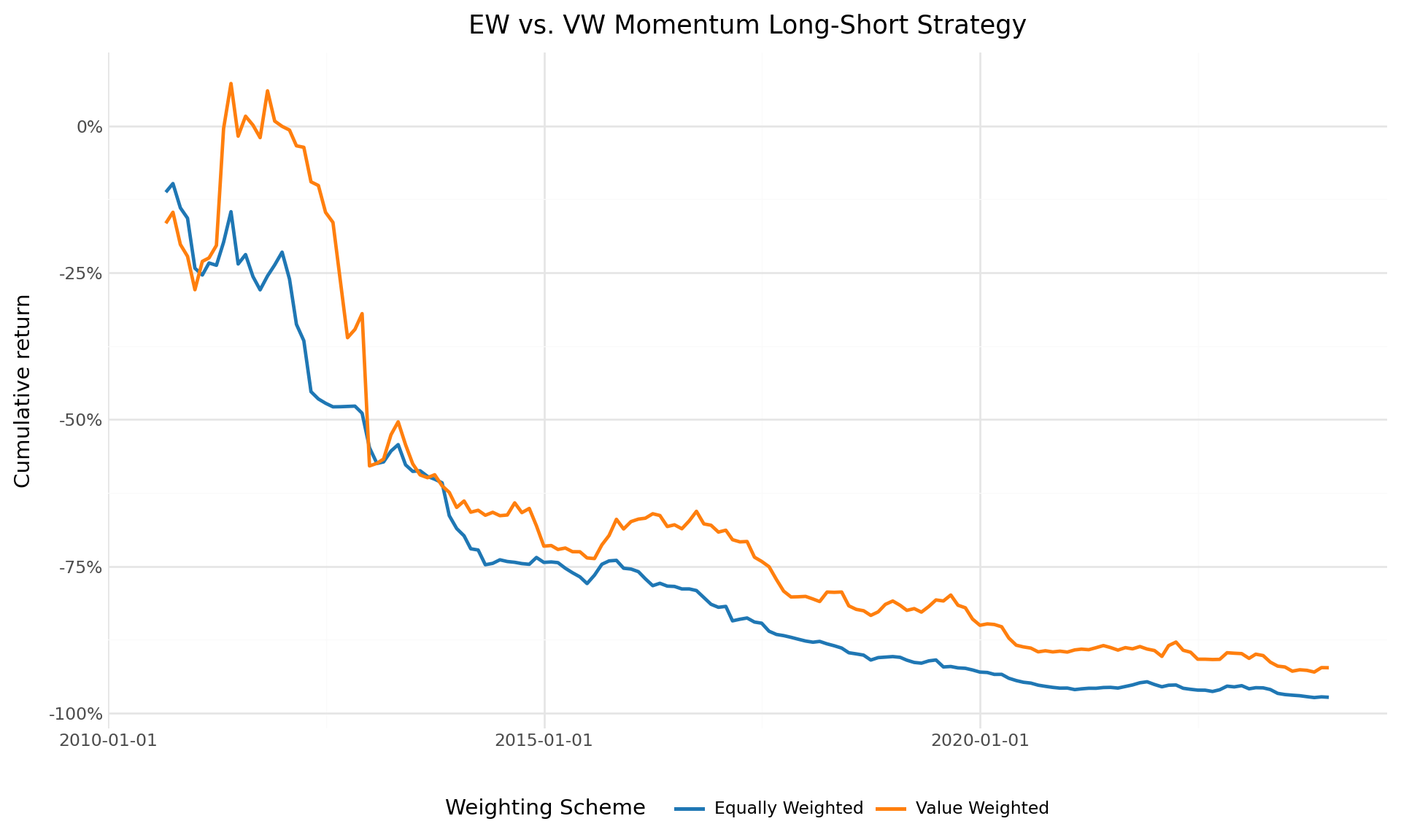
18.11 Daily Momentum Analysis
While momentum strategies are typically evaluated at the monthly frequency following Jegadeesh and Titman (1993), analyzing daily return patterns provides additional insights into the dynamics of momentum profits. Daily data allows us to examine how momentum profits accrue within the holding period, measure intra-month volatility of the strategy, and compute more precise risk measures.
18.11.1 Loading Daily Data
prices_daily = pd.read_sql_query(
    sql=("SELECT symbol, date, ret, ret_excess, mktcap_lag "
         "FROM prices_daily"),
    con=tidy_finance,
    parse_dates={"date"}
)

print(f"Daily observations: {len(prices_daily):,}")
print(f"Unique stocks: {prices_daily['symbol'].nunique():,}")
print(f"Date range: {prices_daily['date'].min().date()} "
      f"to {prices_daily['date'].max().date()}")
Daily observations: 3,462,157
Unique stocks: 1,459
Date range: 2010-01-05 to 2023-12-2918.11.2 Daily Returns of Monthly Momentum Portfolios
Rather than forming momentum portfolios at the daily frequency (which would require daily rebalancing and is impractical), we use the monthly portfolio assignments and track their daily returns. This gives us the daily return series of the monthly momentum strategy.
# # # Use the monthly portfolio assignments from the J=6 baseline
monthly_assignments = portfolios_with_dates[
    ["symbol", "form_date", "momr", "hdate1", "hdate2"]
].copy()

# Merge with daily returns
daily_mom_returns = monthly_assignments.merge(
    prices_daily[["symbol", "date", "ret"]].rename(
        columns={"ret": "dret", "date": "ddate"}
    ),
    on="symbol",
    how="inner"
)

# Use boolean indexing instead of query
daily_mom_returns = daily_mom_returns[
    (daily_mom_returns["ddate"] >= daily_mom_returns["hdate1"]) &
    (daily_mom_returns["ddate"] <= daily_mom_returns["hdate2"])
]

print(f"Daily portfolio return observations: {len(daily_mom_returns):,}")
Daily portfolio return observations: 19,112,536# Compute daily equally weighted portfolio returns
# Stage 1: Average within each cohort
daily_cohort_ret = (daily_mom_returns
.groupby(["ddate", "momr", "form_date"])
.agg(cohort_ret=("dret", "mean"))
.reset_index()
)
# Stage 2: Average across cohorts
daily_ewret = (daily_cohort_ret
.groupby(["ddate", "momr"])
.agg(ewret=("cohort_ret", "mean"))
.reset_index()
.rename(columns={"ddate": "date"})
)
# Compute daily long-short returns
daily_wide = daily_ewret.pivot(
index="date", columns="momr", values="ewret"
).reset_index()
daily_wide.columns = ["date"] + [f"port{i}" for i in range(1, 11)]
daily_wide["winners"] = daily_wide["port10"]
daily_wide["losers"] = daily_wide["port1"]
daily_wide["long_short"] = daily_wide["winners"] - daily_wide["losers"]
print(f"Daily long-short return observations: {len(daily_wide):,}")Daily long-short return observations: 3,35218.11.3 Daily Cumulative Returns
daily_wide = daily_wide.sort_values("date")
daily_wide["cumret_ls"] = (1 + daily_wide["long_short"]).cumprod() - 1

plot_daily_cumret = (
    ggplot(daily_wide, aes(x="date", y="cumret_ls")) +
    geom_line(size=0.5, color="#2ca02c") +
    geom_hline(yintercept=0, linetype="dashed", color="gray") +
    scale_y_continuous(labels=percent_format()) +
    labs(
        x="", y="Cumulative return",
        title="Daily Cumulative Return: Momentum Long-Short Strategy"
    ) +
    theme_minimal() +
    theme(figure_size=(10, 6))
)
plot_daily_cumret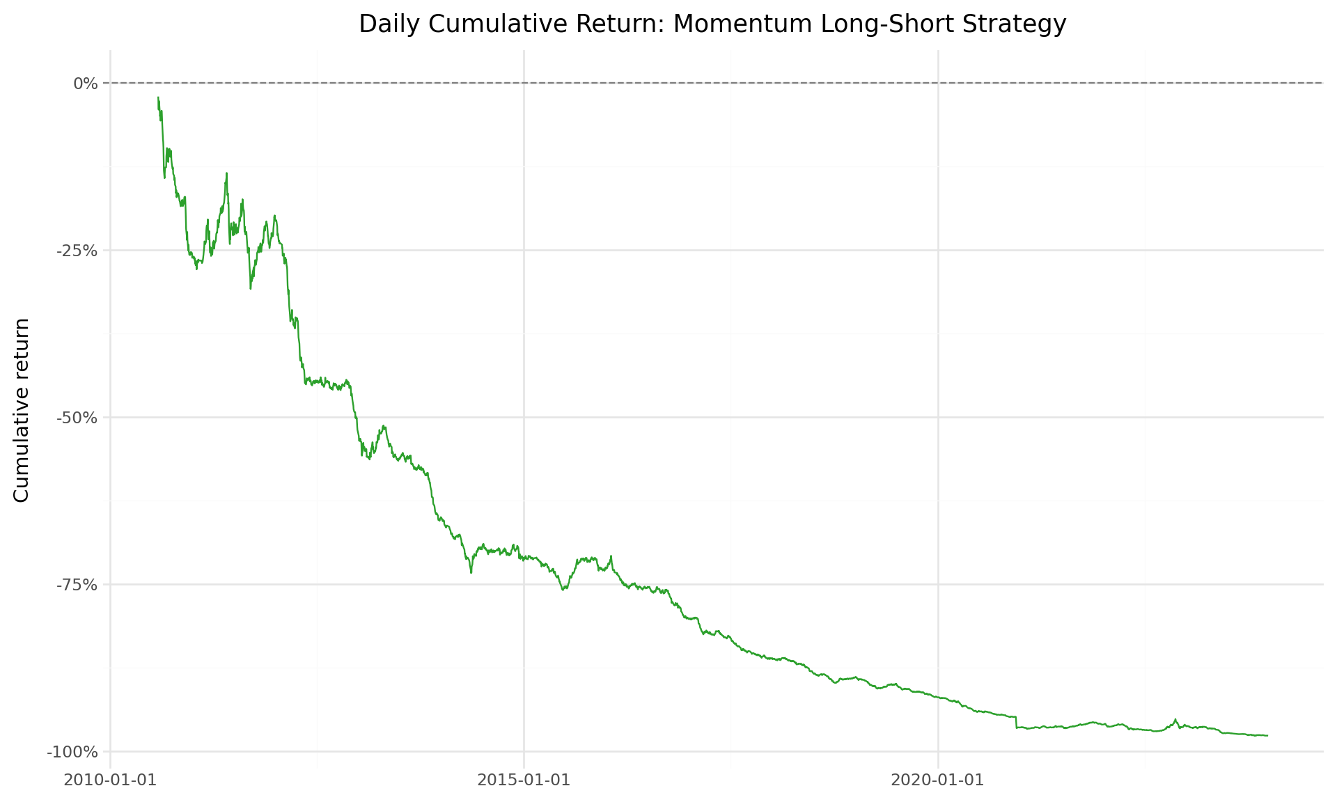
18.11.4 Annualized Risk Metrics from Daily Data
Daily data enables more precise estimation of risk metrics through higher-frequency sampling.
daily_ls = daily_wide["long_short"].dropna()

# Annualized metrics
ann_mean = daily_ls.mean() * 252
ann_vol = daily_ls.std() * np.sqrt(252)
sharpe = ann_mean / ann_vol if ann_vol > 0 else np.nan

# Drawdown
daily_wealth = (1 + daily_ls).cumprod()
daily_running_max = daily_wealth.cummax()
daily_dd = (daily_wealth / daily_running_max - 1).min()

# Higher moments
skew = daily_ls.skew()
kurt = daily_ls.kurtosis()

# VaR and CVaR
var_95 = daily_ls.quantile(0.05)
cvar_95 = daily_ls[daily_ls <= var_95].mean()

risk_metrics = pd.DataFrame({
    "Metric": [
        "Annualized Mean Return",
        "Annualized Volatility",
        "Sharpe Ratio",
        "Maximum Drawdown",
        "Skewness",
        "Excess Kurtosis",
        "Daily VaR (5%)",
        "Daily CVaR (5%)"
    ],
    "Value": [
        f"{ann_mean*100:.2f}%",
        f"{ann_vol*100:.2f}%",
        f"{sharpe:.2f}",
        f"{daily_dd*100:.2f}%",
        f"{skew:.2f}",
        f"{kurt:.2f}",
        f"{var_95*100:.2f}%",
        f"{cvar_95*100:.2f}%"
    ]
})
risk_metrics| Metric | Value | |
|---|---|---|
| 0 | Annualized Mean Return | -26.90% |
| 1 | Annualized Volatility | 15.01% |
| 2 | Sharpe Ratio | -1.79 |
| 3 | Maximum Drawdown | -97.62% |
| 4 | Skewness | -11.23 |
| 5 | Excess Kurtosis | 378.11 |
| 6 | Daily VaR (5%) | -1.33% |
| 7 | Daily CVaR (5%) | -2.10% |
18.11.5 Realized Volatility of Momentum Returns
Using daily returns, we can compute the monthly realized volatility of the momentum strategy and examine how it varies over time.
daily_wide["year_month"] = daily_wide["date"].dt.to_period("M")

realized_vol = (daily_wide
    .groupby("year_month")["long_short"]
    .std()
    .reset_index()
    .rename(columns={"long_short": "realized_vol"})
)
realized_vol["date"] = realized_vol["year_month"].dt.to_timestamp()
realized_vol["realized_vol_ann"] = realized_vol["realized_vol"] * np.sqrt(252)

plot_rvol = (
    ggplot(realized_vol, aes(x="date", y="realized_vol_ann")) +
    geom_line(color="#d62728", size=0.8) +
    scale_y_continuous(labels=percent_format()) +
    labs(
        x="", y="Annualized Realized Volatility",
        title="Realized Volatility of Momentum Strategy"
    ) +
    theme_minimal() +
    theme(figure_size=(10, 5))
)
plot_rvol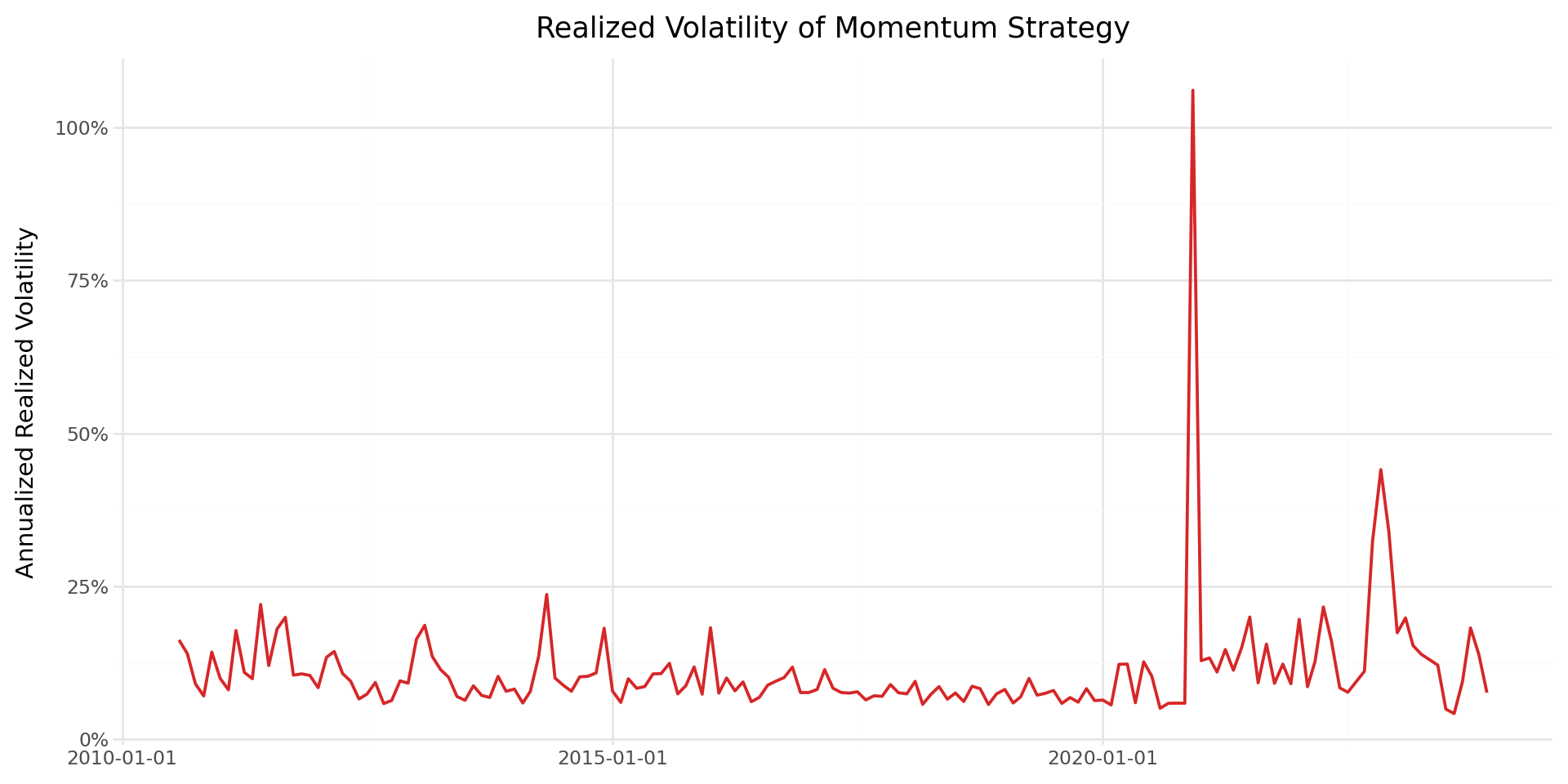
18.12 Saving Results to the Database
We save the momentum portfolio returns to our database for use in subsequent chapters, including factor model construction and portfolio optimization.
# Save monthly equally weighted momentum portfolio returns
ewret_to_save = ewret[["date", "momr", "ewret"]].copy()
ewret_to_save.to_sql(
    name="momentum_portfolios_monthly",
    con=tidy_finance,
    if_exists="replace",
    index=False
)
print(f"Saved {len(ewret_to_save):,} monthly momentum portfolio observations.")

# Save the long-short return series
momentum_factor = ewret_wide[["date", "long_short"]].dropna().copy()
momentum_factor = momentum_factor.rename(columns={"long_short": "wml"})
momentum_factor.to_sql(
    name="momentum_factor_monthly",
    con=tidy_finance,
    if_exists="replace",
    index=False
)
print(f"Saved {len(momentum_factor):,} monthly WML factor observations.")

# Save the daily long-short return series
daily_momentum_factor = daily_wide[["date", "long_short"]].dropna().copy()
daily_momentum_factor = daily_momentum_factor.rename(
    columns={"long_short": "wml"}
)
daily_momentum_factor.to_sql(
    name="momentum_factor_daily",
    con=tidy_finance,
    if_exists="replace",
    index=False
)
print(f"Saved {len(daily_momentum_factor):,} daily WML factor observations.")
Saved 1,610 monthly momentum portfolio observations.
Saved 161 monthly WML factor observations.
Saved 3,352 daily WML factor observations.18.13 Practical Considerations
18.13.1 Transaction Costs
Momentum strategies involve substantial portfolio turnover, as stocks enter and exit the extreme decile portfolios each month. Korajczyk and Sadka (2004) examine whether momentum profits survive transaction costs and find that profitability declines significantly for large institutional investors, though smaller portfolios can still capture meaningful returns.
In the Vietnamese market, transaction costs include:
- Brokerage commissions: Typically 0.15%–0.25% of transaction value for institutional investors.
- Exchange fees: Approximately 0.03% per trade.
- Market impact: Particularly relevant for smaller, less liquid stocks that dominate the extreme momentum portfolios. Vietnam’s lower liquidity compared to developed markets may amplify this cost.
- Trading band limits: The \(\pm 7\%\) daily price limit on HOSE can prevent immediate execution of trades, introducing tracking error relative to the theoretical portfolio.
18.13.2 Implementation Lag
Our baseline implementation assumes that portfolios can be formed and rebalanced instantaneously at the end of each month. In practice, there is a lag between observing the formation period returns and executing the portfolio trades. The one-month gap between the formation period and the start of the holding period (Jegadeesh (1990)) partially addresses this concern, but practitioners should consider additional implementation delays.
18.13.3 Survivorship Bias
Our dataset from DataCore includes both active and delisted stocks, which mitigates survivorship bias. However, the treatment of delisted stocks can affect momentum results. Stocks that are delisted during the holding period may generate extreme returns (both positive for acquisitions and negative for failures). We retain delisted returns as reported in the database, which is consistent with the treatment in Jegadeesh and Titman (1993).
18.13.4 Small Sample Considerations
The Vietnamese stock market has a relatively short history compared to the U.S. market studied in Jegadeesh and Titman (1993). Our sample spans approximately two decades, compared to the nearly three decades in the original study. This shorter sample period implies wider confidence intervals and greater sensitivity to specific episodes (such as the 2007–2009 financial crisis, which had a severe impact on Vietnamese equities). Results should be interpreted with this caveat in mind.
18.14 Key Takeaways
This chapter has provided an implementation and analysis of momentum strategies in the Vietnamese equity market, following the methodology of Jegadeesh and Titman (1993). The main findings and methodological contributions are:
Methodology: We implemented the full Jegadeesh and Titman (1993) overlapping portfolio methodology, including the two-stage averaging procedure (within-cohort, then across-cohort) that handles the \(K\) active portfolios in each month.
Baseline results: The \(J=6\), \(K=6\) strategy provides a natural benchmark. The spread between winner and loser portfolios reveals whether cross-sectional momentum exists in Vietnamese equities.
Robustness across horizons: By computing the full \(J \times K\) grid with \(J, K \in \{3, 6, 9, 12\}\), we assessed whether the momentum premium is robust to the choice of formation and holding periods, following the approach in Jegadeesh and Titman (1993) Table 1.
Risk adjustment: CAPM and Fama-French three-factor alphas measure whether the momentum premium is explained by standard risk factors, building on the analysis in Fama and French (1996) who show that their three-factor model fails to explain momentum.
Market state dependence: Following Cooper, Gutierrez Jr, and Hameed (2004), we examined whether momentum profits vary with market conditions, which is particularly relevant in emerging markets with pronounced boom-bust cycles.
Value weighting: The comparison of equally weighted and value-weighted strategies addresses practical implementability and isolates the role of firm size in driving momentum profits.
Daily analysis: By tracking momentum portfolios at the daily frequency, we computed precise risk metrics including realized volatility, maximum drawdown, VaR, and CVaR, providing a complete risk profile of the strategy.
Emerging market context: Throughout the analysis, we have highlighted features specific to the Vietnamese market—trading band limits, foreign ownership restrictions, shorter sample history, and higher transaction costs—that affect the interpretation and practical viability of momentum strategies.