Show code
import pandas as pd
import numpy as np
from scipy import stats
from scipy.optimize import minimize
import plotnine as p9
from mizani.formatters import percent_format, comma_format
import warnings
warnings.filterwarnings("ignore")Finance is fundamentally a discipline of extremes. The central objects of concern (e.g., asset pricing, portfolio allocation, capital regulation, systemic stability) are all disproportionately shaped by rare but severe events. A portfolio manager who correctly estimates the mean and variance of returns but ignores the possibility of a \(-20\%\) daily move is, in the language of Taleb (2010), “picking up pennies in front of a steamroller.” The 1997 Asian Financial Crisis, the 2008 Global Financial Crisis, and the 2020 COVID-19 crash each demonstrated that the most consequential realizations in financial markets are precisely those that conventional Gaussian models assign near-zero probability.
This chapter develops the statistical and econometric toolkit for measuring, modeling, and diagnosing tail risk in Vietnamese equity markets. We focus on three interconnected layers. First, at the individual stock level, we estimate crash risk measures that capture the asymmetry and thickness of the left tail of return distributions. Second, at the portfolio or regulatory level, we implement Value at Risk (VaR) and Expected Shortfall (ES) under multiple estimation approaches and evaluate their accuracy via backtesting. Third, at the system level, we apply Extreme Value Theory (EVT) and tail dependence measures to characterize joint crash behavior across sectors and assess financial contagion.
Vietnamese markets present a particularly rich laboratory for studying tail phenomena. Daily price limits mechanically censor the tails of observed return distributions, creating latent tail risk that is not directly observable but must be inferred. State ownership concentrations, thin liquidity, and herding behavior among retail investors amplify crash dynamics. The absence of a developed derivatives market means that tail hedging instruments familiar in more developed markets (e.g., deep out-of-the-money puts, variance swaps) are largely unavailable, making accurate tail risk measurement all the more important for risk management.
The return distribution of individual stocks and market indices is not symmetric. Decades of evidence, beginning with Mandelbrot et al. (1963) and formalized in the asset pricing context by Harvey and Siddique (2000), establish that equity returns exhibit negative skewness (i.e., large negative returns occur more frequently than a Gaussian model predicts) and excess kurtosis (i.e., the tails are thicker than normal in both directions, but the left tail is of primary economic concern).
Let \(r_{i,t}\) denote the daily log return of stock \(i\) on day \(t\). The standardized third central moment (skewness) is:
\[ \text{Skew}(r_i) = \frac{E\left[(r_{i,t} - \mu_i)^3\right]}{\sigma_i^3} \tag{43.1}\]
Negative skewness implies that the distribution has a longer or fatter left tail relative to the right. In economic terms, negative skewness means that large losses are more likely than large gains of equal magnitude. The standardized fourth moment (excess kurtosis) is:
\[ \text{Kurt}(r_i) = \frac{E\left[(r_{i,t} - \mu_i)^4\right]}{\sigma_i^4} - 3 \tag{43.2}\]
Positive excess kurtosis indicates heavier tails than the normal distribution. Both moments have direct asset pricing implications: Harvey and Siddique (2000) and Kraus and Litzenberger (1976) argue that investors demand compensation for holding negatively skewed assets, implying that crash-prone stocks should earn higher expected returns, ceteris paribus.
The literature has developed several firm-specific crash risk measures. We implement the three most widely used, following Chen, Hong, and Stein (2001) and Hutton, Marcus, and Tehranian (2009).
Measure 1: Negative Coefficient of Skewness (NCSKEW)
For each firm \(i\) in fiscal year \(y\), compute firm-specific weekly returns \(W_{i,\tau}\) as residuals from a market model augmented with lead and lag market returns to account for nonsynchronous trading:
\[ r_{i,t} = \alpha_i + \beta_{1i} r_{m,t-1} + \beta_{2i} r_{m,t} + \beta_{3i} r_{m,t+1} + \varepsilon_{i,t} \tag{43.3}\]
where \(r_{m,t}\) is the value-weighted market return on day \(t\). The firm-specific weekly return is \(W_{i,\tau} = \ln(1 + \sum_{t \in \tau} \hat{\varepsilon}_{i,t})\), where \(\tau\) indexes weeks. NCSKEW is then:
\[ \text{NCSKEW}_{i,y} = -\frac{n(n-1)^{3/2} \sum W_{i,\tau}^3}{(n-1)(n-2)\left(\sum W_{i,\tau}^2\right)^{3/2}} \tag{43.4}\]
where \(n\) is the number of firm-specific weekly returns in the year. The negative sign ensures that higher NCSKEW corresponds to greater crash risk.
Measure 2: Down-to-Up Volatility (DUVOL)
Partition the firm-specific weekly returns into “down weeks” (\(W_{i,\tau} < \bar{W}_i\)) and “up weeks” (\(W_{i,\tau} \geq \bar{W}_i\)), where \(\bar{W}_i\) is the annual mean. Then:
\[ \text{DUVOL}_{i,y} = \ln\left(\frac{(n_u - 1)\sum_{\text{down}} W_{i,\tau}^2}{(n_d - 1)\sum_{\text{up}} W_{i,\tau}^2}\right) \tag{43.5}\]
where \(n_u\) and \(n_d\) are the number of up and down weeks, respectively. Higher DUVOL indicates greater crash risk. Chen, Hong, and Stein (2001) argue that DUVOL is less sensitive to outliers than NCSKEW because it does not involve the cube of returns.
Measure 3: Crash Count (COUNT)
Define a crash event as a firm-specific weekly return that falls below \(k\) standard deviations of its annual distribution:
\[ \text{CRASH}_{i,\tau} = \mathbb{1}\left(W_{i,\tau} < \bar{W}_i - k \cdot \hat{\sigma}_{W_i}\right) \tag{43.6}\]
The standard threshold in the literature is \(k = 3.09\), corresponding to the 0.1% tail of a standard normal distribution. The crash count for year \(y\) is \(\text{COUNT}_{i,y} = \sum_{\tau \in y} \text{CRASH}_{i,\tau}\).
# DataCore.vn API
from datacore import DataCore
dc = DataCore()
# Load daily stock returns and market returns
daily_returns = dc.get_daily_returns(
start_date="2010-01-01",
end_date="2024-12-31"
)
# Market return: value-weighted index
market_returns = dc.get_market_returns(
start_date="2010-01-01",
end_date="2024-12-31",
frequency="daily"
)
# Merge
df = daily_returns.merge(
market_returns[["date", "mkt_ret"]],
on="date",
how="left"
)
print(f"Universe: {df['ticker'].nunique()} firms, "
f"{df['date'].nunique()} trading days")from sklearn.linear_model import LinearRegression
def compute_firm_specific_returns(group):
"""
Estimate firm-specific daily returns from augmented market model
with lead and lag market returns (Chen, Hong, Stein 2001).
"""
g = group.sort_values("date").copy()
g["mkt_lag1"] = g["mkt_ret"].shift(1)
g["mkt_lead1"] = g["mkt_ret"].shift(-1)
g = g.dropna(subset=["ret", "mkt_ret", "mkt_lag1", "mkt_lead1"])
if len(g) < 30:
return pd.DataFrame()
X = g[["mkt_lag1", "mkt_ret", "mkt_lead1"]].values
y = g["ret"].values
model = LinearRegression().fit(X, y)
g["resid"] = y - model.predict(X)
return g[["ticker", "date", "resid"]]
# Estimate by firm-year
df["year"] = df["date"].dt.year
firm_resids = (
df.groupby(["ticker", "year"], group_keys=False)
.apply(compute_firm_specific_returns)
.reset_index(drop=True)
)# Aggregate daily residuals to weekly firm-specific returns
firm_resids["date"] = pd.to_datetime(firm_resids["date"])
firm_resids["week"] = firm_resids["date"].dt.isocalendar().week.astype(int)
firm_resids["year"] = firm_resids["date"].dt.year
weekly_returns = (
firm_resids.groupby(["ticker", "year", "week"])
.agg(W=("resid", lambda x: np.log(1 + x.sum())))
.reset_index()
)def compute_crash_measures(group):
"""Compute NCSKEW, DUVOL, and CRASH count for one firm-year."""
W = group["W"].values
n = len(W)
if n < 26: # Require at least 26 weeks
return pd.Series({
"ncskew": np.nan, "duvol": np.nan,
"crash_count": np.nan, "n_weeks": n
})
# NCSKEW
W_demean = W - W.mean()
num = n * (n - 1)**1.5 * np.sum(W_demean**3)
den = (n - 1) * (n - 2) * (np.sum(W_demean**2))**1.5
ncskew = -(num / den) if den != 0 else np.nan
# DUVOL
mean_W = W.mean()
down = W[W < mean_W]
up = W[W >= mean_W]
n_d, n_u = len(down), len(up)
if n_d > 1 and n_u > 1:
duvol = np.log(
((n_u - 1) * np.sum(down**2)) /
((n_d - 1) * np.sum(up**2))
)
else:
duvol = np.nan
# Crash count (k = 3.09)
threshold = W.mean() - 3.09 * W.std()
crash_count = int(np.sum(W < threshold))
return pd.Series({
"ncskew": ncskew,
"duvol": duvol,
"crash_count": crash_count,
"n_weeks": n
})
crash_risk = (
weekly_returns.groupby(["ticker", "year"])
.apply(compute_crash_measures)
.reset_index()
)
crash_risk = crash_risk.dropna(subset=["ncskew", "duvol"])
print(f"Crash risk panel: {len(crash_risk)} firm-years")Table 43.1 presents summary statistics for the three crash risk measures across the Vietnamese equity market.
plot_data = crash_risk[crash_risk["year"].between(2012, 2024)].copy()
(
p9.ggplot(plot_data, p9.aes(x="ncskew"))
+ p9.geom_histogram(bins=50, fill="#2E5090", alpha=0.7)
+ p9.facet_wrap("~year", scales="free_y", ncol=4)
+ p9.geom_vline(xintercept=0, linetype="dashed", color="red", size=0.5)
+ p9.labs(
x="NCSKEW",
y="Count",
title="Distribution of Firm-Level Crash Risk (NCSKEW)"
)
+ p9.theme_minimal()
+ p9.theme(figure_size=(12, 8))
)The rightward shift of the NCSKEW distribution during crisis episodes, particularly in 2020 and 2022, indicates a market-wide increase in crash risk. The red dashed line at zero separates firms with negative skewness (right of zero, i.e., high NCSKEW since the measure is negated) from those with positive skewness.
Crash risk has first-order implications for asset pricing. Harvey and Siddique (2000) demonstrate that coskewness (i.e., the contribution of an individual asset to the skewness of the aggregate market portfolio) is priced in the cross-section of expected returns. Specifically, assets that tend to crash when the market crashes (negative coskewness) should command a risk premium.
The coskewness of stock \(i\) with the market is:
\[ \text{CoSkew}_i = \frac{E\left[(r_i - \mu_i)(r_m - \mu_m)^2\right]}{\sigma_i \cdot \sigma_m^2} \tag{43.7}\]
Stocks with more negative coskewness exhibit disproportionately poor performance during market downturns. In Vietnam, this is especially relevant because: (1) retail investor herding amplifies co-movement during selloffs; (2) price limits delay crash completion, spreading crash risk across multiple days; and (3) state-owned enterprises, which constitute a large fraction of market capitalization, may exhibit coordinated crash behavior driven by common policy shocks.
def compute_coskewness(group):
"""Estimate coskewness for a firm-year."""
r_i = group["ret"].values
r_m = group["mkt_ret"].values
if len(r_i) < 60:
return np.nan
r_i_dm = r_i - r_i.mean()
r_m_dm = r_m - r_m.mean()
coskew = (
np.mean(r_i_dm * r_m_dm**2) /
(np.std(r_i) * np.std(r_m)**2)
)
return coskew
df_coskew = (
df.groupby(["ticker", "year"])
.apply(lambda g: pd.Series({"coskewness": compute_coskewness(g)}))
.reset_index()
.dropna()
)median_coskew = (
df_coskew.groupby("year")
.agg(
median_coskew=("coskewness", "median"),
q25=("coskewness", lambda x: x.quantile(0.25)),
q75=("coskewness", lambda x: x.quantile(0.75))
)
.reset_index()
)
(
p9.ggplot(median_coskew, p9.aes(x="year"))
+ p9.geom_ribbon(
p9.aes(ymin="q25", ymax="q75"),
fill="#2E5090", alpha=0.2
)
+ p9.geom_line(p9.aes(y="median_coskew"), color="#2E5090", size=1)
+ p9.geom_hline(yintercept=0, linetype="dashed", color="gray")
+ p9.labs(
x="Year",
y="Coskewness",
title="Cross-Sectional Coskewness: Median and Interquartile Range"
)
+ p9.theme_minimal()
+ p9.theme(figure_size=(10, 5))
)Beyond skewness, the concentration of returns in the extreme left tail provides additional diagnostic information. We define the downside tail concentration ratio as the fraction of total return variance attributable to observations below the \(p\)-th percentile:
\[ \text{TCR}_p = \frac{\sum_{r_{i,t} < q_p} (r_{i,t} - \bar{r}_i)^2}{\sum_t (r_{i,t} - \bar{r}_i)^2} \tag{43.8}\]
where \(q_p\) is the \(p\)-th percentile of the firm’s return distribution. Under a symmetric distribution, \(\text{TCR}_{5\%}\) would be close to \(5\%\) (with a slight upward bias due to the squaring). Values substantially exceeding \(5\%\) indicate that the left tail contributes disproportionately to total risk.
def tail_concentration_ratio(returns, p=0.05):
"""Compute tail concentration ratio at percentile p."""
q = np.quantile(returns, p)
r_dm = returns - returns.mean()
total_var = np.sum(r_dm**2)
tail_var = np.sum(r_dm[returns < q]**2)
return tail_var / total_var if total_var > 0 else np.nan
tcr = (
df.groupby(["ticker", "year"])
.agg(
tcr_5=("ret", lambda x: tail_concentration_ratio(x.values, 0.05)),
tcr_1=("ret", lambda x: tail_concentration_ratio(x.values, 0.01)),
n_obs=("ret", "count")
)
.reset_index()
.query("n_obs >= 120")
)
print("Median TCR(5%):", round(tcr["tcr_5"].median(), 4))
print("Median TCR(1%):", round(tcr["tcr_1"].median(), 4))Value at Risk (VaR) and Expected Shortfall (ES) are the two principal quantile-based risk measures used in financial regulation and internal risk management. For a portfolio return \(r\) with the cumulative distribution function \(F\), the VaR at confidence level \(\alpha\) is:
\[ \text{VaR}_\alpha = -F^{-1}(\alpha) = -\inf\{x : F(x) \geq \alpha\} \tag{43.9}\]
This is simply the negative of the \(\alpha\)-quantile of the return distribution. For \(\alpha = 0.01\), \(\text{VaR}_{1\%}\) answers: “What is the loss that is exceeded with only 1% probability?”
Expected Shortfall (also called Conditional VaR or CVaR) is the expected loss conditional on the loss exceeding VaR:
\[ \text{ES}_\alpha = -\frac{1}{\alpha}\int_0^\alpha F^{-1}(u) \, du = -E\left[r \mid r \leq -\text{VaR}_\alpha\right] \tag{43.10}\]
For continuous distributions, ES simplifies to the conditional expectation in Equation 43.10. ES is always at least as large as VaR (\(\text{ES}_\alpha \geq \text{VaR}_\alpha\)) and is strictly larger whenever the distribution has any mass beyond the VaR quantile.
Table 43.2 summarizes the fundamental differences.
| Property | VaR | Expected Shortfall |
|---|---|---|
| Definition | Quantile of the loss distribution | Conditional mean loss beyond VaR |
| Tail information | None beyond the quantile | Captures severity of tail losses |
| Subadditivity | Not subadditive in general | Subadditive (coherent risk measure) |
| Regulatory status | Basel II primary measure | Basel III/IV primary measure |
| Backtesting | Binary: breach or no breach | Continuous: requires severity assessment |
| Sensitivity to tail shape | None | Directly sensitive |
The critical deficiency of VaR is the absence of subadditivity. A risk measure \(\rho\) is subadditive if \(\rho(X + Y) \leq \rho(X) + \rho(Y)\) for all portfolios \(X, Y\). VaR violates this condition for non-elliptical distributions, meaning that diversification can appear to increase risk under VaR, which is a perverse result. Artzner et al. (1999) established the axiomatic framework for coherent risk measures, and ES satisfies all four axioms: monotonicity, translation invariance, positive homogeneity, and subadditivity. VaR satisfies only three.
We implement four approaches to VaR and ES estimation, each with distinct assumptions and data requirements.
Method 1: Historical Simulation
The simplest nonparametric approach uses the empirical distribution directly:
\[ \widehat{\text{VaR}}_\alpha^{\text{HS}} = -\hat{F}_n^{-1}(\alpha) = -r_{(\lceil n\alpha \rceil)} \tag{43.11}\]
where \(r_{(k)}\) is the \(k\)-th order statistic of the return sample. ES is the average of all returns below the VaR:
\[ \widehat{\text{ES}}_\alpha^{\text{HS}} = -\frac{1}{\lfloor n\alpha \rfloor}\sum_{k=1}^{\lfloor n\alpha \rfloor} r_{(k)} \tag{43.12}\]
Method 2: Parametric (Gaussian)
Assume \(r_t \sim N(\mu, \sigma^2)\). Then:
\[ \text{VaR}_\alpha^{\text{Gauss}} = -(\hat{\mu} + \hat{\sigma} \cdot \Phi^{-1}(\alpha)) \tag{43.13}\]
\[ \text{ES}_\alpha^{\text{Gauss}} = -\hat{\mu} + \hat{\sigma} \cdot \frac{\phi(\Phi^{-1}(\alpha))}{\alpha} \tag{43.14}\]
where \(\Phi\) and \(\phi\) are the standard normal CDF and PDF, respectively. The Gaussian assumption is known to underestimate tail risk for equity returns, but provides a useful baseline.
Method 3: Parametric (Student-\(t\))
The Student-\(t\) distribution with \(\nu\) degrees of freedom captures excess kurtosis. The VaR and ES are:
\[ \text{VaR}_\alpha^{t} = -\left(\hat{\mu} + \hat{\sigma}\sqrt{\frac{\nu - 2}{\nu}} \cdot t_\nu^{-1}(\alpha)\right) \tag{43.15}\]
\[ \text{ES}_\alpha^{t} = -\hat{\mu} + \hat{\sigma}\sqrt{\frac{\nu-2}{\nu}} \cdot \frac{f_{t_\nu}(t_\nu^{-1}(\alpha))}{\alpha} \cdot \frac{\nu + (t_\nu^{-1}(\alpha))^2}{\nu - 1} \tag{43.16}\]
where \(t_\nu^{-1}\) and \(f_{t_\nu}\) are the quantile function and PDF of the Student-\(t\) distribution.
Method 4: GARCH-Filtered EVT (Semi-Parametric)
This approach, developed by McNeil and Frey (2000), first filters returns through a GARCH(1,1) model to obtain standardized residuals \(z_t = \hat{\varepsilon}_t / \hat{\sigma}_t\), then fits a Generalized Pareto Distribution (GPD) to the lower tail of the standardized residuals. We detail the EVT component in Section 43.3.
def estimate_var_es(returns, alpha=0.01):
"""
Estimate VaR and ES at level alpha using four methods.
Parameters
----------
returns : array-like
Return series.
alpha : float
Tail probability (e.g., 0.01 for 1%).
Returns
-------
dict : VaR and ES estimates for each method.
"""
r = np.array(returns)
r = r[~np.isnan(r)]
n = len(r)
mu, sigma = r.mean(), r.std(ddof=1)
results = {}
# Method 1: Historical simulation
sorted_r = np.sort(r)
idx = int(np.ceil(n * alpha))
results["var_hs"] = -sorted_r[idx - 1]
results["es_hs"] = -sorted_r[:idx].mean()
# Method 2: Gaussian
z_alpha = stats.norm.ppf(alpha)
results["var_gauss"] = -(mu + sigma * z_alpha)
results["es_gauss"] = -mu + sigma * stats.norm.pdf(z_alpha) / alpha
# Method 3: Student-t (MLE for degrees of freedom)
try:
nu, loc, scale = stats.t.fit(r)
t_alpha = stats.t.ppf(alpha, df=nu)
results["var_t"] = -(loc + scale * t_alpha)
results["es_t"] = (
-loc + scale *
(stats.t.pdf(t_alpha, df=nu) / alpha) *
((nu + t_alpha**2) / (nu - 1))
)
results["nu_hat"] = nu
except Exception:
results["var_t"] = np.nan
results["es_t"] = np.nan
results["nu_hat"] = np.nan
return results# Compute VaR and ES for the aggregate market index
market_daily = dc.get_market_returns(
start_date="2010-01-01",
end_date="2024-12-31",
frequency="daily"
)
# Rolling 1-year VaR/ES
window = 252
results_list = []
for end_idx in range(window, len(market_daily)):
window_returns = market_daily["mkt_ret"].iloc[end_idx - window:end_idx].values
date = market_daily["date"].iloc[end_idx]
est = estimate_var_es(window_returns, alpha=0.01)
est["date"] = date
results_list.append(est)
var_es_ts = pd.DataFrame(results_list)plot_var = var_es_ts.melt(
id_vars="date",
value_vars=["var_hs", "var_gauss", "var_t"],
var_name="method",
value_name="var"
)
method_labels = {
"var_hs": "Historical Simulation",
"var_gauss": "Gaussian",
"var_t": "Student-t"
}
plot_var["method"] = plot_var["method"].map(method_labels)
(
p9.ggplot(plot_var, p9.aes(x="date", y="var", color="method"))
+ p9.geom_line(alpha=0.8, size=0.6)
+ p9.labs(
x="", y="1% VaR (Loss)",
title="Rolling 252-Day Value at Risk Estimates",
color="Method"
)
+ p9.scale_color_manual(
values=["#2E5090", "#C0392B", "#27AE60"]
)
+ p9.theme_minimal()
+ p9.theme(figure_size=(12, 5), legend_position="top")
)plot_es = var_es_ts.melt(
id_vars="date",
value_vars=["es_hs", "es_gauss", "es_t"],
var_name="method",
value_name="es"
)
method_labels_es = {
"es_hs": "Historical Simulation",
"es_gauss": "Gaussian",
"es_t": "Student-t"
}
plot_es["method"] = plot_es["method"].map(method_labels_es)
(
p9.ggplot(plot_es, p9.aes(x="date", y="es", color="method"))
+ p9.geom_line(alpha=0.8, size=0.6)
+ p9.labs(
x="", y="1% ES (Loss)",
title="Rolling 252-Day Expected Shortfall Estimates",
color="Method"
)
+ p9.scale_color_manual(
values=["#2E5090", "#C0392B", "#27AE60"]
)
+ p9.theme_minimal()
+ p9.theme(figure_size=(12, 5), legend_position="top")
)A VaR model is only useful if its predictions are accurate. Backtesting evaluates whether the realized frequency of VaR breaches is consistent with the nominal confidence level. If VaR is estimated at the \(\alpha = 1\%\) level, we expect approximately 1% of days to exhibit losses exceeding VaR.
The Kupiec unconditional coverage test (Kupiec et al. 1995) evaluates whether the total number of breaches \(x\) in \(n\) observations is consistent with \(\alpha\):
\[ \text{LR}_{\text{UC}} = -2\ln\left(\frac{\alpha^x (1-\alpha)^{n-x}}{\hat{p}^x (1-\hat{p})^{n-x}}\right) \sim \chi^2(1) \tag{43.17}\]
where \(\hat{p} = x/n\) is the empirical breach frequency. The Christoffersen conditional coverage test (Christoffersen 1998) additionally evaluates whether breaches are independent (no clustering):
\[ \text{LR}_{\text{CC}} = \text{LR}_{\text{UC}} + \text{LR}_{\text{IND}} \tag{43.18}\]
where \(\text{LR}_{\text{IND}}\) tests the null of independence using a first-order Markov chain model for breach indicators.
def kupiec_test(returns, var_estimates, alpha=0.01):
"""
Kupiec unconditional coverage test for VaR backtesting.
Returns
-------
dict : breach count, expected, breach rate, LR statistic, p-value.
"""
breaches = returns < -var_estimates
x = breaches.sum()
n = len(returns)
p_hat = x / n
if p_hat == 0 or p_hat == 1:
return {"breaches": x, "expected": n * alpha,
"breach_rate": p_hat, "lr_stat": np.nan, "p_value": np.nan}
lr = -2 * (
x * np.log(alpha) + (n - x) * np.log(1 - alpha)
- x * np.log(p_hat) - (n - x) * np.log(1 - p_hat)
)
p_value = 1 - stats.chi2.cdf(lr, df=1)
return {
"breaches": int(x),
"expected": round(n * alpha, 1),
"breach_rate": round(p_hat, 4),
"lr_stat": round(lr, 4),
"p_value": round(p_value, 4)
}
# Backtest each method
actual_returns = market_daily["mkt_ret"].iloc[window:].values
backtest_results = {}
for method, col in [("Historical", "var_hs"),
("Gaussian", "var_gauss"),
("Student-t", "var_t")]:
backtest_results[method] = kupiec_test(
actual_returns, var_es_ts[col].values, alpha=0.01
)
bt_df = pd.DataFrame(backtest_results).T
bt_df.index.name = "Method"
bt_dfIn Vietnamese equity markets, many stocks have short trading histories, thin liquidity, and censored returns due to price limits. These features create challenges for tail risk estimation that are less severe in developed markets.
Price limit censoring. When a stock hits its daily price limit, the observed return is truncated. The true latent return may extend well beyond the limit, but is unobservable. This means that historical simulation mechanically understates VaR and ES for stocks that frequently hit limits. A Tobit-type correction can partially address this:
\[ r_{i,t}^{\text{latent}} \sim N(\mu_i, \sigma_i^2), \quad r_{i,t}^{\text{obs}} = \max(\underline{L}, \min(\bar{L}, r_{i,t}^{\text{latent}})) \tag{43.19}\]
The parameters \((\mu_i, \sigma_i^2)\) can be estimated via maximum likelihood on the censored sample, and VaR/ES can then be computed from the estimated latent distribution.
Short histories. For recently listed stocks, the available sample may be too short for reliable nonparametric estimation. In these cases, shrinkage toward a cross-sectional prior (e.g., the sector median VaR) or Bayesian approaches with informative priors can improve stability.
GARCH models capture volatility clustering (i.e., the tendency of large returns to be followed by large returns), but they make specific distributional assumptions about standardized residuals (typically Gaussian or Student-\(t\)). The tail behavior of the conditional distribution is thus determined by the parametric innovation assumption, not learned from the data.
Extreme Value Theory (EVT) takes a fundamentally different approach. It provides a statistical framework for estimating the distribution of extreme observations without specifying the entire return distribution. The key theoretical results (i.e., the Fisher-Tippett-Gnedenko theorem and the Pickands-Balkema-de Haan theorem) establish that the distribution of properly normalized maxima (or exceedances over high thresholds) converges to specific parametric families regardless of the parent distribution. This universality is what makes EVT powerful: the tail can be estimated even when the center of the distribution is misspecified.
The tail index \(\xi\) (also denoted \(\alpha^{-1}\) in some formulations) governs the rate of tail decay. For heavy-tailed distributions, the survival function satisfies:
\[ P(X > x) \sim L(x) \cdot x^{-1/\xi}, \quad x \to \infty \tag{43.20}\]
where \(L(x)\) is a slowly varying function. The tail index \(\xi > 0\) implies a Pareto-type tail; larger \(\xi\) means heavier tails. Financial return distributions typically have \(\xi \in (0.2, 0.5)\), corresponding to tail indices \(\alpha = 1/\xi \in (2, 5)\), which implies finite variance but potentially infinite higher moments.
The Hill estimator (Hill 1975) provides a simple nonparametric estimate of \(\xi\) from the upper order statistics:
\[ \hat{\xi}_{\text{Hill}}(k) = \frac{1}{k}\sum_{j=1}^{k} \ln X_{(n-j+1)} - \ln X_{(n-k)} \tag{43.21}\]
where \(X_{(1)} \leq \cdots \leq X_{(n)}\) are the order statistics and \(k\) is the number of upper order statistics used. The choice of \(k\) involves a bias-variance tradeoff: small \(k\) yields high variance; large \(k\) introduces bias from non-tail observations.
def hill_estimator(data, k_values=None):
"""
Compute Hill estimator of tail index for a range of k values.
Parameters
----------
data : array-like
Positive values (use absolute values of losses).
k_values : array-like, optional
Number of upper order statistics to use.
Returns
-------
DataFrame with columns [k, xi_hat, se].
"""
x = np.sort(np.abs(data))[::-1] # Descending order
n = len(x)
if k_values is None:
k_values = range(10, min(n // 2, 500), 5)
results = []
for k in k_values:
if k >= n or k < 2:
continue
log_excess = np.log(x[:k]) - np.log(x[k])
xi_hat = log_excess.mean()
se = xi_hat / np.sqrt(k)
results.append({"k": k, "xi_hat": xi_hat, "se": se})
return pd.DataFrame(results)# Use negative market returns (losses)
losses = -market_daily["mkt_ret"].dropna().values
losses_positive = losses[losses > 0]
hill_results = hill_estimator(losses_positive)
(
p9.ggplot(hill_results, p9.aes(x="k", y="xi_hat"))
+ p9.geom_ribbon(
p9.aes(ymin="xi_hat - 1.96 * se", ymax="xi_hat + 1.96 * se"),
fill="#2E5090", alpha=0.2
)
+ p9.geom_line(color="#2E5090", size=0.8)
+ p9.geom_hline(yintercept=0.33, linetype="dashed", color="red")
+ p9.annotate(
"text", x=hill_results["k"].max() * 0.7, y=0.35,
label="ξ = 1/3 (cubic tail)", color="red", size=8
)
+ p9.labs(
x="Number of Order Statistics (k)",
y="Hill Estimate ξ̂",
title="Hill Plot for Market Return Left Tail"
)
+ p9.theme_minimal()
+ p9.theme(figure_size=(10, 5))
)The Hill plot is a standard diagnostic in EVT. A stable region of the Hill estimate across a range of \(k\) suggests a reliable tail index estimate. The red dashed line at \(\xi = 1/3\) corresponds to a tail index of \(\alpha = 3\), which implies that the third moment (skewness) is infinite, which is a finding consistent with much of the empirical finance literature (Cont 2001; Gabaix et al. 2003).
The Fisher-Tippett-Gnedenko theorem establishes that if the maximum of \(n\) i.i.d. random variables, after proper normalization, converges in distribution, the limit must be a Generalized Extreme Value (GEV) distribution:
\[ G_\xi(x) = \exp\left\{-\left(1 + \xi \cdot \frac{x - \mu}{\sigma}\right)^{-1/\xi}\right\} \tag{43.22}\]
for \(1 + \xi(x - \mu)/\sigma > 0\), where \(\mu\) is the location, \(\sigma > 0\) the scale, and \(\xi\) the shape parameter. The three sub-families are in Table 43.3.
| Shape \(\xi\) | Distribution | Tail Type | Finance Example |
|---|---|---|---|
| \(\xi > 0\) | Fréchet | Heavy (polynomial decay) | Equity returns, credit losses |
| \(\xi = 0\) | Gumbel | Light (exponential decay) | Normal/lognormal models |
| \(\xi < 0\) | Weibull | Bounded upper tail | Bounded loss distributions |
For the block maxima approach, we divide the return series into non-overlapping blocks (typically months or quarters) and extract the minimum return (maximum loss) from each block. The GEV is then fitted to these block minima.
from scipy.stats import genextreme
# Monthly block minima (maximum losses)
market_daily["month"] = market_daily["date"].dt.to_period("M")
block_minima = (
market_daily.groupby("month")
.agg(min_ret=("mkt_ret", "min"))
.reset_index()
)
# Fit GEV to negated block minima (so we model maxima of losses)
block_losses = -block_minima["min_ret"].values
xi_hat, loc_hat, scale_hat = genextreme.fit(block_losses)
print(f"GEV fit to monthly block maxima of losses:")
print(f" Shape (ξ): {xi_hat:.4f}")
print(f" Location (μ): {loc_hat:.4f}")
print(f" Scale (σ): {scale_hat:.4f}")x_grid = np.linspace(
block_losses.min() * 0.8,
block_losses.max() * 1.2,
200
)
gev_pdf = genextreme.pdf(x_grid, xi_hat, loc=loc_hat, scale=scale_hat)
plot_data = pd.DataFrame({
"x": np.concatenate([block_losses, x_grid]),
"source": (["Empirical"] * len(block_losses) +
["GEV Fit"] * len(x_grid)),
"density": np.concatenate([
np.full(len(block_losses), np.nan),
gev_pdf
]),
"value": np.concatenate([block_losses, np.full(len(x_grid), np.nan)])
})
empirical = plot_data[plot_data["source"] == "Empirical"]
fitted = plot_data[plot_data["source"] == "GEV Fit"]
(
p9.ggplot()
+ p9.geom_histogram(
data=empirical, mapping=p9.aes(x="value", y="..density.."),
bins=30, fill="#2E5090", alpha=0.5
)
+ p9.geom_line(
data=fitted, mapping=p9.aes(x="x", y="density"),
color="#C0392B", size=1
)
+ p9.labs(
x="Monthly Maximum Loss",
y="Density",
title="GEV Distribution Fit to Monthly Block Maxima"
)
+ p9.theme_minimal()
+ p9.theme(figure_size=(10, 5))
)The Peaks Over Threshold (POT) approach is generally preferred over block maxima because it uses tail data more efficiently. The Pickands-Balkema-de Haan theorem establishes that for a sufficiently high threshold \(u\), the distribution of exceedances \(Y = X - u \mid X > u\) converges to a Generalized Pareto Distribution (GPD):
\[ H_{\xi,\beta}(y) = \begin{cases} 1 - \left(1 + \frac{\xi y}{\beta}\right)^{-1/\xi} & \text{if } \xi \neq 0 \\ 1 - \exp\left(-\frac{y}{\beta}\right) & \text{if } \xi = 0 \end{cases} \tag{43.23}\]
for \(y > 0\) and \(1 + \xi y / \beta > 0\), where \(\beta > 0\) is the scale parameter and \(\xi\) is the shape parameter (identical to the GEV shape). The POT-based VaR and ES at level \(\alpha\) are:
\[ \text{VaR}_\alpha^{\text{GPD}} = u + \frac{\hat{\beta}}{\hat{\xi}}\left[\left(\frac{n}{N_u} \cdot \alpha\right)^{-\hat{\xi}} - 1\right] \tag{43.24}\]
\[ \text{ES}_\alpha^{\text{GPD}} = \frac{\text{VaR}_\alpha^{\text{GPD}}}{1 - \hat{\xi}} + \frac{\hat{\beta} - \hat{\xi} u}{1 - \hat{\xi}} \tag{43.25}\]
where \(N_u\) is the number of observations exceeding \(u\) and \(n\) is the total sample size. These formulae are valid for \(\hat{\xi} < 1\).
from scipy.stats import genpareto
def fit_gpd_pot(returns, threshold_quantile=0.95):
"""
Fit GPD to exceedances over threshold using POT approach.
Parameters
----------
returns : array-like
Return series (losses should be positive).
threshold_quantile : float
Quantile for threshold selection.
Returns
-------
dict : Threshold, GPD parameters, VaR, ES estimates.
"""
losses = -np.array(returns)
losses = losses[~np.isnan(losses)]
n = len(losses)
u = np.quantile(losses, threshold_quantile)
exceedances = losses[losses > u] - u
N_u = len(exceedances)
# Fit GPD
xi_hat, _, beta_hat = genpareto.fit(exceedances, floc=0)
# VaR and ES at 1%
alpha = 0.01
var_gpd = u + (beta_hat / xi_hat) * (
(n / N_u * alpha)**(-xi_hat) - 1
)
es_gpd = var_gpd / (1 - xi_hat) + (beta_hat - xi_hat * u) / (1 - xi_hat)
return {
"threshold": u,
"n_exceedances": N_u,
"xi_hat": xi_hat,
"beta_hat": beta_hat,
"var_1pct": var_gpd,
"es_1pct": es_gpd
}
# Fit GPD to market losses
gpd_results = fit_gpd_pot(market_daily["mkt_ret"].dropna().values, 0.95)
print("GPD-POT Results (1% level):")
for k, v in gpd_results.items():
if isinstance(v, float):
print(f" {k}: {v:.6f}")
else:
print(f" {k}: {v}")The choice of threshold \(u\) is the key practical decision in POT analysis. Too low a threshold violates the asymptotic approximation; too high wastes data. The mean residual life plot provides a graphical diagnostic: if the GPD approximation holds above \(u_0\), the mean excess function \(e(u) = E[X - u \mid X > u]\) is linear in \(u\) for \(u > u_0\):
\[ e(u) = \frac{\beta + \xi u}{1 - \xi} \tag{43.26}\]
losses = -market_daily["mkt_ret"].dropna().values
losses_sorted = np.sort(losses)
thresholds = np.quantile(losses, np.linspace(0.80, 0.99, 50))
mean_excess = []
for u in thresholds:
exceedances = losses[losses > u] - u
if len(exceedances) > 5:
mean_excess.append({
"threshold": u,
"mean_excess": exceedances.mean(),
"se": exceedances.std() / np.sqrt(len(exceedances)),
"n_exceed": len(exceedances)
})
mrl_df = pd.DataFrame(mean_excess)
(
p9.ggplot(mrl_df, p9.aes(x="threshold", y="mean_excess"))
+ p9.geom_ribbon(
p9.aes(
ymin="mean_excess - 1.96 * se",
ymax="mean_excess + 1.96 * se"
),
fill="#2E5090", alpha=0.2
)
+ p9.geom_line(color="#2E5090", size=0.8)
+ p9.geom_point(color="#2E5090", size=1.5)
+ p9.labs(
x="Threshold (u)",
y="Mean Excess e(u)",
title="Mean Residual Life Plot"
)
+ p9.theme_minimal()
+ p9.theme(figure_size=(10, 5))
)A threshold in the region where the mean residual life plot is approximately linear is appropriate. In practice, we also compare GPD parameter stability across a range of thresholds and select the lowest threshold at which estimates stabilize.
Table 43.4 summarizes the complementary roles of these two modeling frameworks.
| Feature | GARCH | EVT |
|---|---|---|
| What is modeled | Conditional variance dynamics | Unconditional tail distribution |
| Distributional assumption | Full distribution (Gaussian or \(t\)) | Only the tail (GPD or GEV) |
| Time dependence | Explicit (volatility clustering) | None (i.i.d. or filtered) |
| Tail shape | Determined by innovation distribution | Estimated from data |
| Extreme quantiles | Extrapolation from parametric assumption | Principled extrapolation via EVT theorems |
| Best use | Short-horizon risk forecasting | Extreme quantile estimation, stress testing |
The GARCH-filtered EVT approach of McNeil and Frey (2000) combines both: GARCH captures the time-varying volatility, and EVT models the residual tail. This hybrid approach is considered best practice for financial risk management (McNeil, Frey, and Embrechts 2015).
Perhaps the most important practical fact about multivariate tail risk is that correlations estimated from the body of the distribution systematically understate dependence in the tails. Longin and Solnik (2001) demonstrate this using extreme value theory: for bivariate normal returns, the correlation of extreme realizations converges to zero as the threshold moves further into the tail. Yet empirically, the correlation of crash returns remains large and often increases (a phenomenon incompatible with multivariate normality).
Formally, the coefficient of lower tail dependence between two return series \(X\) and \(Y\) is:
\[ \lambda_L = \lim_{q \to 0^+} P\left(Y \leq F_Y^{-1}(q) \mid X \leq F_X^{-1}(q)\right) \tag{43.27}\]
If \(\lambda_L > 0\), the two series exhibit asymptotic tail dependence (i.e., extreme losses tend to occur jointly). For the bivariate normal distribution, \(\lambda_L = 0\) for all \(|\rho| < 1\) (asymptotic tail independence). This means that any model built on multivariate normality will structurally underestimate the probability of joint crashes. The Student-\(t\) copula, by contrast, has \(\lambda_L > 0\) for \(\rho > -1\), which is why it has become the workhorse model for joint tail risk in finance (Demarta and McNeil 2005).
We implement several empirical measures of joint crash behavior.
Exceedance Correlation. Following Longin and Solnik (2001), compute the correlation of returns conditional on both returns falling below a threshold \(\theta\):
\[ \rho^-(\theta) = \text{Corr}(r_i, r_j \mid r_i < \theta, r_j < \theta) \tag{43.28}\]
If returns are bivariate normal, \(\rho^-(\theta) \to 0\) as \(\theta \to -\infty\). Empirically, \(\rho^-(\theta)\) typically increases as \(\theta\) decreases, indicating tail dependence beyond what the normal model implies.
Co-Exceedance Count. For each day \(t\), count the number of stocks or sectors whose returns fall below the \(q\)-th percentile of their respective marginal distributions:
\[ C_t(q) = \sum_{i=1}^{N} \mathbb{1}\left(r_{i,t} < F_i^{-1}(q)\right) \tag{43.29}\]
Days with high \(C_t(q)\) represent system-wide stress events.
def empirical_tail_dependence(x, y, quantiles=None):
"""
Estimate lower tail dependence coefficient at various quantiles.
Uses the empirical copula approach: transform to uniform margins,
then estimate P(V <= q | U <= q) for decreasing q.
"""
if quantiles is None:
quantiles = [0.20, 0.15, 0.10, 0.05, 0.03, 0.01]
# Transform to uniform margins via empirical CDF
from scipy.stats import rankdata
n = len(x)
u = rankdata(x) / (n + 1)
v = rankdata(y) / (n + 1)
results = []
for q in quantiles:
mask_u = u <= q
mask_both = mask_u & (v <= q)
n_u = mask_u.sum()
n_both = mask_both.sum()
lambda_hat = n_both / n_u if n_u > 0 else np.nan
results.append({
"quantile": q,
"lambda_L": lambda_hat,
"n_below_x": int(n_u),
"n_co_crash": int(n_both)
})
return pd.DataFrame(results)# Load sector-level daily returns
sector_returns = dc.get_sector_returns(
start_date="2010-01-01",
end_date="2024-12-31",
frequency="daily"
)
# Compute pairwise tail dependence for major sectors
sectors = sector_returns["sector"].unique()[:8] # Top 8 sectors
import itertools
pairwise_td = []
for s1, s2 in itertools.combinations(sectors, 2):
r1 = sector_returns.loc[
sector_returns["sector"] == s1, ["date", "ret"]
].set_index("date")["ret"]
r2 = sector_returns.loc[
sector_returns["sector"] == s2, ["date", "ret"]
].set_index("date")["ret"]
# Align dates
aligned = pd.concat([r1, r2], axis=1, join="inner").dropna()
if len(aligned) < 500:
continue
td = empirical_tail_dependence(
aligned.iloc[:, 0].values,
aligned.iloc[:, 1].values,
quantiles=[0.05]
)
pairwise_td.append({
"sector_1": s1,
"sector_2": s2,
"lambda_L_5pct": td["lambda_L"].iloc[0],
"pearson_corr": aligned.iloc[:, 0].corr(aligned.iloc[:, 1])
})
td_df = pd.DataFrame(pairwise_td)td_display = td_df.copy()
td_display["lambda_L_5pct"] = td_display["lambda_L_5pct"].round(4)
td_display["pearson_corr"] = td_display["pearson_corr"].round(4)
td_display["ratio"] = (
td_display["lambda_L_5pct"] / td_display["pearson_corr"]
).round(3)
td_display.sort_values("lambda_L_5pct", ascending=False).head(15)The ratio column in Table 43.5 is particularly informative. When \(\lambda_L / \rho \gg 1\), the sectors exhibit disproportionately high co-crash frequency relative to their overall correlation. This is the hallmark of tail dependence that Gaussian models miss.
To assess system-wide contagion dynamics, we construct daily co-exceedance counts and examine their time-series properties.
# Compute daily co-exceedance count at the 5% level
sector_wide = sector_returns.pivot_table(
index="date", columns="sector", values="ret"
)
# Rolling 252-day quantile thresholds
quantile_thresholds = sector_wide.rolling(252, min_periods=60).quantile(0.05)
# Indicator: return below rolling 5th percentile
exceedance_indicators = (sector_wide < quantile_thresholds).astype(int)
co_exceedance = exceedance_indicators.sum(axis=1)
co_exceedance.name = "co_exceedance"
co_exceed_df = co_exceedance.reset_index()
co_exceed_df.columns = ["date", "co_exceedance"]
co_exceed_df["n_sectors"] = exceedance_indicators.notna().sum(axis=1).values(
p9.ggplot(co_exceed_df.dropna(), p9.aes(x="date", y="co_exceedance"))
+ p9.geom_line(color="#2E5090", alpha=0.5, size=0.3)
+ p9.geom_smooth(method="lowess", color="#C0392B", size=1, se=False)
+ p9.labs(
x="",
y="Number of Sectors in Left Tail",
title="System-Wide Stress: Daily Co-Exceedance Count"
)
+ p9.theme_minimal()
+ p9.theme(figure_size=(12, 5))
)Peaks in the co-exceedance series correspond to system-wide stress episodes. The smoothed trend (red line) reveals the evolving baseline level of systemic fragility.
The literature distinguishes several channels through which stress propagates across assets, sectors, and markets (Forbes and Rigobon 2002; Kaminsky, Reinhart, and Vegh 2002):
Direct linkages. Balance sheet interconnections, interbank lending, and cross-holdings create direct transmission channels. When institution \(A\) holds assets issued by institution \(B\), losses at \(B\) directly impair \(A\)’s balance sheet.
Information contagion. Adverse news about one firm triggers reassessment of similarly exposed firms. King and Wadhwani (1990) and Kodres and Pritsker (2002) formalize this via Bayesian updating: investors cannot distinguish idiosyncratic from systematic shocks, so a crash in one asset leads them to update beliefs about common risk factors.
Liquidity contagion. Fire sales by distressed institutions depress prices of commonly held assets, creating losses for other holders. Markus K. Brunnermeier (2009) model this as a liquidity spiral: declining prices trigger margin calls, which force further sales, further depressing prices. In Vietnamese markets, the absence of circuit breakers beyond price limits and the concentration of holdings among a few large institutional investors amplify this channel.
Behavioral contagion. Herding behavior (i.e., investors mimicking others’ trades) generates correlated selling pressure even in the absence of fundamental linkages. Bikhchandani, Hirshleifer, and Welch (1992) and Banerjee (1992) provide theoretical foundations. Choe, Kho, and Stulz (2005) document herding in emerging markets specifically.
We can test for contagion (as distinct from interdependence) using the Forbes and Rigobon (2002) framework. The null hypothesis is that the co-movement observed during a crisis period is fully explained by the increase in volatility (which mechanically inflates correlations). The adjusted correlation is:
\[ \rho^* = \frac{\rho_{\text{crisis}}}{\sqrt{1 + \delta[1 - \rho_{\text{crisis}}^2]}} \tag{43.30}\]
where \(\delta = \sigma_{\text{crisis}}^2 / \sigma_{\text{tranquil}}^2 - 1\) is the relative increase in variance. If \(\rho^* > \rho_{\text{tranquil}}\), the increase in co-movement exceeds what volatility adjustment alone predicts, which is evidence of contagion.
def forbes_rigobon_test(returns_df, crisis_start, crisis_end):
"""
Forbes-Rigobon adjusted correlation test for contagion.
Parameters
----------
returns_df : DataFrame
Columns are sector returns, index is date.
crisis_start, crisis_end : str
Crisis period boundaries.
Returns
-------
DataFrame : Pairwise contagion test results.
"""
tranquil = returns_df[returns_df.index < crisis_start].dropna()
crisis = returns_df[
(returns_df.index >= crisis_start) &
(returns_df.index <= crisis_end)
].dropna()
sectors = returns_df.columns.tolist()
results = []
for s1, s2 in itertools.combinations(sectors, 2):
if s1 not in tranquil.columns or s2 not in crisis.columns:
continue
rho_t = tranquil[s1].corr(tranquil[s2])
rho_c = crisis[s1].corr(crisis[s2])
var_t = tranquil[s1].var()
var_c = crisis[s1].var()
if var_t == 0:
continue
delta = var_c / var_t - 1
rho_adj = rho_c / np.sqrt(1 + delta * (1 - rho_c**2))
results.append({
"sector_1": s1,
"sector_2": s2,
"rho_tranquil": round(rho_t, 4),
"rho_crisis": round(rho_c, 4),
"rho_adjusted": round(rho_adj, 4),
"contagion": rho_adj > rho_t
})
return pd.DataFrame(results)# Test for contagion during COVID-19 crash
contagion_covid = forbes_rigobon_test(
sector_wide,
crisis_start="2020-02-01",
crisis_end="2020-04-30"
)
n_pairs = len(contagion_covid)
n_contagion = contagion_covid["contagion"].sum()
print(f"COVID-19 contagion test: {n_contagion}/{n_pairs} sector pairs "
f"show evidence of contagion ({100*n_contagion/n_pairs:.1f}%)")We construct several market-wide stress indicators that aggregate the individual-level and sectoral tail risk measures developed above into a comprehensive system-level diagnostic.
Aggregate Crash Risk Index. The cross-sectional average of firm-level NCSKEW provides a market-wide measure of crash risk that is forward-looking (it captures the buildup of negative skewness before a crash materializes):
\[ \text{ACRI}_y = \frac{1}{N_y}\sum_{i=1}^{N_y} \text{NCSKEW}_{i,y} \tag{43.31}\]
Market Tail Risk (MTR). Following Kelly and Jiang (2014), we estimate the time-varying tail risk of the market portfolio using option-implied or realized tail measures. In the absence of a liquid options market in Vietnam, we use the realized version based on the Hill tail index estimated from rolling windows:
\[ \text{MTR}_t = \hat{\xi}_t^{\text{Hill}} \cdot \hat{\sigma}_t \tag{43.32}\]
where \(\hat{\xi}_t^{\text{Hill}}\) is the Hill estimator computed from a trailing 252-day window and \(\hat{\sigma}_t\) is the conditional volatility (e.g., from GARCH). This interaction captures both the thickness of the tail and the current scale of volatility.
# Aggregate Crash Risk Index
acri = (
crash_risk.groupby("year")
.agg(
acri=("ncskew", "mean"),
median_ncskew=("ncskew", "median"),
pct_high_crash=("ncskew", lambda x: (x > x.quantile(0.75)).mean()),
n_firms=("ncskew", "count")
)
.reset_index()
)
# Market Tail Risk: rolling Hill estimator x rolling volatility
mkt_returns = market_daily["mkt_ret"].dropna().values
dates = market_daily["date"].dropna().values
mtr_list = []
for end_idx in range(504, len(mkt_returns)):
window_ret = mkt_returns[end_idx - 252:end_idx]
losses_pos = -window_ret[window_ret < 0]
if len(losses_pos) < 30:
continue
# Hill estimator at k = 50
sorted_losses = np.sort(losses_pos)[::-1]
k = min(50, len(sorted_losses) - 1)
if k < 10:
continue
log_excess = np.log(sorted_losses[:k]) - np.log(sorted_losses[k])
xi_hat = log_excess.mean()
sigma_hat = window_ret.std()
mtr = xi_hat * sigma_hat
mtr_list.append({
"date": dates[end_idx],
"xi_hat": xi_hat,
"sigma_hat": sigma_hat,
"mtr": mtr
})
mtr_df = pd.DataFrame(mtr_list)
mtr_df["date"] = pd.to_datetime(mtr_df["date"])(
p9.ggplot(mtr_df, p9.aes(x="date", y="mtr"))
+ p9.geom_line(color="#2E5090", alpha=0.5, size=0.4)
+ p9.geom_smooth(method="lowess", color="#C0392B", size=1, se=False)
+ p9.labs(
x="",
y="MTR (ξ × σ)",
title="Market Tail Risk: Rolling Hill Index × Conditional Volatility"
)
+ p9.theme_minimal()
+ p9.theme(figure_size=(12, 5))
)Not all sectors are equally vulnerable to tail events. We decompose system-wide tail risk into sectoral contributions to identify the most fragile parts of the market.
# Sector-level tail statistics
sector_tail_stats = []
for sector in sectors:
sector_data = sector_returns[sector_returns["sector"] == sector]["ret"].dropna()
if len(sector_data) < 500:
continue
s_data = sector_data.values
# Skewness and kurtosis
skew = stats.skew(s_data)
kurt = stats.kurtosis(s_data)
# VaR and ES at 1%
var_1 = -np.quantile(s_data, 0.01)
es_1 = -s_data[s_data <= np.quantile(s_data, 0.01)].mean()
# Hill tail index (k=50)
losses_pos = -s_data[s_data < 0]
sorted_l = np.sort(losses_pos)[::-1]
k = min(50, len(sorted_l) - 1)
if k >= 10:
log_exc = np.log(sorted_l[:k]) - np.log(sorted_l[k])
xi = log_exc.mean()
else:
xi = np.nan
sector_tail_stats.append({
"sector": sector,
"skewness": round(skew, 3),
"excess_kurtosis": round(kurt, 3),
"var_1pct": round(var_1, 4),
"es_1pct": round(es_1, 4),
"tail_index_xi": round(xi, 3) if not np.isnan(xi) else np.nan,
"n_obs": len(s_data)
})
fragility_df = pd.DataFrame(sector_tail_stats)(
p9.ggplot(
fragility_df.dropna(),
p9.aes(x="tail_index_xi", y="es_1pct", label="sector")
)
+ p9.geom_point(color="#2E5090", size=3)
+ p9.geom_text(nudge_y=0.002, size=7)
+ p9.labs(
x="Tail Index (ξ, Hill)",
y="1% Expected Shortfall",
title="Sector Fragility Map"
)
+ p9.theme_minimal()
+ p9.theme(figure_size=(10, 7))
)Sectors in the upper-right quadrant of Figure 43.10 exhibit both high expected shortfall (large average losses in the tail) and high tail index (heavier-than-typical tails). These represent the most fragile components of the market from a systemic stability perspective.
We construct a comprehensive crisis diagnostic framework that combines the indicators developed above to identify, characterize, and compare stress episodes in Vietnamese financial markets.
# Identify extreme co-exceedance days (system-wide stress events)
threshold_high_stress = co_exceed_df["co_exceedance"].quantile(0.99)
stress_events = co_exceed_df[
co_exceed_df["co_exceedance"] >= threshold_high_stress
].copy()
# Add market return on stress days
stress_events = stress_events.merge(
market_daily[["date", "mkt_ret"]], on="date", how="left"
)
print(f"System-wide stress days (top 1%): {len(stress_events)}")
print(f"Average market return on stress days: "
f"{stress_events['mkt_ret'].mean():.4f}")
print(f"Average co-exceedance on stress days: "
f"{stress_events['co_exceedance'].mean():.1f}")# Cluster stress days into episodes (within 10 trading days)
stress_events = stress_events.sort_values("date").reset_index(drop=True)
stress_events["gap"] = stress_events["date"].diff().dt.days
stress_events["episode"] = (stress_events["gap"] > 15).cumsum()
episode_summary = (
stress_events.groupby("episode")
.agg(
start_date=("date", "min"),
end_date=("date", "max"),
n_stress_days=("date", "count"),
avg_market_return=("mkt_ret", "mean"),
min_market_return=("mkt_ret", "min"),
avg_coexceedance=("co_exceedance", "mean")
)
.reset_index(drop=True)
.sort_values("min_market_return")
)
episode_summary["avg_market_return"] = episode_summary["avg_market_return"].round(4)
episode_summary["min_market_return"] = episode_summary["min_market_return"].round(4)
episode_summary["avg_coexceedance"] = episode_summary["avg_coexceedance"].round(1)
episode_summary.head(10)The diagnostics above identify when the system is under stress from prices alone. They say nothing about who moves first, how fast the exit propagates, and who is left holding the losses. Those questions are usually unanswerable because bank deposit records are confidential. Liu, Makarov, and Schoar (2026) answer them for one of the largest runs of the past decade by exploiting a setting where every transaction is public: the collapse of the Terra ecosystem in May 2022, which erased roughly $50 billion of value in three days. Terra’s algorithmic stablecoin, UST, was convertible one-for-one into $1 of the network’s native token, LUNA, so in economic terms UST was perpetual convertible debt backed by LUNA. Demand for UST came almost entirely from Anchor, a lending protocol that paid depositors a fixed 19.5% yield when comparable stablecoin rates elsewhere were 2 to 3%. The authors reconstruct the full transaction history of 3.7 million addresses across the Terra blockchain, Ethereum bridges, and centralized exchanges, and their account of the episode reads like a field guide to bank runs.
Four findings are worth carrying into any study of Vietnamese financial stability.
Fragility was built before the trigger, and it was visible. Anchor’s yield was never covered by borrowing income; a yield reserve topped up by the sponsor covered the gap, and the reserve was draining from December 2021. UST supply rose from 2.5 billion to 18.5 billion in six months, most of it parked in Anchor, while the market value of LUNA that backed it was falling. Depositor entry rates dropped and exit rates rose from April 2022, weeks before the crash. This is the sunspot-plus-fundamentals structure of the global-games literature: weak fundamentals turn an innocuous public signal into a coordination device. The signals that ended up coordinating the run were a scheduled rebalancing of a liquidity pool and the moment LUNA’s market capitalization fell to the level of UST outstanding, a threshold that meant nothing to a fully rational investor but that many participants treated as proof the backing was gone.
The run was not manipulation but a cascade started by a few large depositors. Two wallets withdrew 400 million UST from Anchor on 7 May 2022 and sold on the deepest venues. Other large wallets followed within hours because they could watch the withdrawals on-chain. Anchor deposits fell from 14 billion to under 2 billion UST by 13 May, and the swap mechanism that was supposed to defend the peg instead drove LUNA supply from under 1 billion to 5.89 trillion as investors converted UST to LUNA and sold, the death spiral the design implied.
Transparency did not level the playing field. Addresses with more than 10 million UST withdrew almost everything within two days and lost 26% on average. Addresses below 1,000 UST kept adding deposits until 10 May, trying to buy the dip, and lost 76%. Controlling for size, addresses that had used cross-chain bridges or traded on several exchanges lost significantly less, so sophistication mattered independently of wealth. Everyone could see the same ledger; only some could act on it in time.
A lender of last resort works only while the liability is small. UST had de-pegged once before, in May 2021, and recovered because the sponsor and an allied trading firm absorbed the selling when UST outstanding was a few hundred million. In May 2022 the same actors spent about $2.5 billion defending the peg against 18 billion of claims and failed. The intervention that restores confidence at one scale is a rounding error at the next.
The Vietnamese reading is direct. The deposit run on Saigon Commercial Bank (SCB) in October 2022, which forced the State Bank of Vietnam to place the bank under special control within days of the Vạn Thịnh Phát arrests, and the wave of redemptions from corporate bond funds in the same quarter after the Tân Hoàng Minh and Vạn Thịnh Phát bond cases, share the Terra anatomy: a liability that grew faster than its backing, a yield that only made sense if the sponsor kept paying, a public event that coordinated withdrawals, and a retail base that moved last. Vietnam also has one of the highest rates of retail crypto participation in the world, so a share of Vietnamese households held UST directly and sat on the wrong side of the loss table above. Two research designs follow. First, the crisis-episode table in this section can be extended from prices to flows: daily foreign-investor net sales by ticker, fund NAV redemptions, and, for the 2022 bond episode, the timing of retail versus institutional bondholder exits, to test whether the large-first, small-last ordering holds in Vietnamese data. Second, the co-exceedance measures above are early-warning signals for prices; Liu, Makarov, and Schoar (2026) suggest complementing them with stock measures of fragility, the ratio of short-term claims to liquid backing at each intermediary, because that ratio is what determined whether the same intervention succeeded in 2021 and failed in 2022.
The Terra episode was a run on a liability: depositors withdrew because they expected others to withdraw. Khorrami and Mendo (2026) show that the asset side of a balance sheet can fail in the same self-fulfilling way, and that this fragility survives the remedy usually thought to remove it, namely complete markets for hedging fundamental risk.
Their starting point is the financial-accelerator model of Markus K. Brunnermeier and Sannikov (2014), in the tradition of Kiyotaki and Moore (1997). Productive “experts” earn \(a_e\) per unit of capital and less productive “households” earn \(a_h < a_e\), so capital is worth more in experts’ hands, the same logic by which Shleifer and Vishny (1992) explain why assets sold to outsiders fetch less. Experts cannot issue equity, so they finance capital with their own net worth and short-term debt. In the conventional version, a bad fundamental shock erodes expert net worth, experts sell capital to households, the price of capital falls because the buyers value it less, and the falling price erodes expert net worth further. The standard view is that this accelerator needs unhedged fundamental risk: if experts could insure their balance sheets against the shock, there would be nothing to amplify.
Khorrami and Mendo let agents hedge every fundamental shock frictionlessly. Fundamental shocks then never cause fire sales, and there is an efficient equilibrium in which experts hold all capital and its price evolves deterministically. But some risk is always left unhedged: shocks that are novel, or that hit balance sheets no market lets investors short. Call such a shock a sunspot. If agents expect experts to sell capital when it arrives, the expectation fulfils itself:
Two equations make the loop concrete. Let \(\eta\) be the experts’ share of aggregate wealth, \(\psi\) their share of the capital stock, and \(\bar{\rho}(\eta) = \eta\rho_e + (1-\eta)\rho_h\) the wealth-weighted discount rate. Goods-market clearing ties the price of capital to who holds it,
\[ q\,\bar{\rho}(\eta) = \psi\, a_e + (1-\psi)\, a_h, \tag{43.33}\]
so the price is high only when experts hold the capital. In the region where they do not hold all of it (\(\psi < 1\)), the equilibrium price function satisfies
\[ q'(\eta) = \frac{(a_e - a_h)\, q}{q\,\bar{\rho}(\eta) - \eta\, a_e - (1-\eta)\, a_h}, \qquad \sigma_q^2 = \frac{\eta(1-\eta)}{\psi - \eta}\cdot\frac{a_e - a_h}{q}, \tag{43.34}\]
where \(\sigma_q\) is the volatility of the capital price driven entirely by the sunspot. The second expression is the condition that experts’ extra productivity, \((a_e - a_h)/q\), exactly compensates them for bearing more of the unhedgeable price risk than households do. Once experts are rich enough that \(\psi\) reaches one, the economy behaves like the safe equilibrium and sunspot volatility is zero.
The paper establishes three results that matter beyond the model.
The size of a fire sale is a belief. The differential equation in Equation 43.34 needs a boundary condition: the share of capital experts are believed to keep when their wealth approaches zero, \(\psi_0\). Every \(\psi_0 \in [0, 1)\) supports an equilibrium, from the full fire sale (\(\psi_0 = 0\), experts dump everything when broke) to the safe equilibrium (\(\psi_0 \to 1\)). Greater optimism about how much capital experts will retain in the tail produces smaller fire sales, lower volatility, and higher prices, which justifies the optimism.
Self-fulfilling and fundamental fire sales are observationally equivalent. If fundamental risk is unhedgeable with volatility \(\sigma\), the conventional accelerator equilibrium converges, as \(\sigma \to 0\), to the full fire-sale sunspot equilibrium. This formalizes the “volatility paradox” of Markus K. Brunnermeier and Sannikov (2014): endogenous volatility does not vanish as exogenous risk does. The consequence for empirical work is uncomfortable. Data generated by an economy that amplifies fundamental shocks look the same as data generated by one that coordinates on non-fundamental ones.
The worst equilibrium is selected. If agents perceive the sunspot as having a vanishingly small fundamental effect, and experts face a leverage constraint that is then relaxed, only the full fire-sale equilibrium survives. With jump rather than Brownian shocks, the selected equilibrium features large, discrete fire sales and markedly worse misallocation.
Two further implications distinguish this from a bank run. The fire sale needs no maturity mismatch and no illiquid asset: even fundamentally safe assets can be fire-sold if coordinated selling can depress their price. And because debt is always repaid, deposit insurance has no role. The remedy the authors point to is a credible promise to buy assets in the disaster state, which would raise \(\psi_0\) and remove the worst equilibria, though whether such promises create ex ante moral hazard is left open.
The equilibrium is easy to compute. The code below solves Equation 43.34 for three disaster beliefs, using the parameters of the paper’s numerical example, and compares the result with the safe equilibrium in which \(q = a_e/\bar{\rho}(\eta)\).
from scipy.integrate import solve_ivp
RHO_E, RHO_H = 0.06, 0.04 # discount rates: experts, households
A_E, A_H = 0.11, 0.03 # productivity: experts, households
def rho_bar(eta):
return eta * RHO_E + (1 - eta) * RHO_H
def capital_share(q, eta):
# Price-output relation solved for experts' capital share psi
return (q * rho_bar(eta) - A_H) / (A_E - A_H)
def solve_fire_sale(psi0, eta_max=0.6, n_grid=600):
"""Sunspot equilibrium with disaster belief psi0 = psi(0+)."""
def rhs(eta, y):
q = y[0]
return [(A_E - A_H) * q
/ (q * rho_bar(eta) - eta * A_E - (1 - eta) * A_H)]
if psi0 > 0:
eta_0 = 1e-9
q_0 = (psi0 * A_E + (1 - psi0) * A_H) / rho_bar(eta_0)
else:
# psi0 = 0 is a singular boundary: near it, psi - eta ~ sqrt(2 c eta)
eta_0 = 1e-8
c = A_H / (A_E - A_H)
q_0 = ((eta_0 + np.sqrt(2 * c * eta_0)) * (A_E - A_H) + A_H) \
/ rho_bar(eta_0)
def full_allocation(eta, y): # stop where experts hold everything
return capital_share(y[0], eta) - 1
full_allocation.terminal = True
full_allocation.direction = 1
sol = solve_ivp(rhs, (eta_0, eta_max), [q_0], events=full_allocation,
dense_output=True, rtol=1e-10, atol=1e-12, method="LSODA")
eta_star = sol.t_events[0][0] if sol.t_events[0].size else eta_max
eta = np.linspace(eta_0, eta_max, n_grid)
fire_sale_region = eta < eta_star
q = np.where(fire_sale_region,
sol.sol(np.minimum(eta, eta_star))[0],
A_E / rho_bar(eta))
psi = np.minimum(capital_share(q, eta), 1.0)
sigma_q = np.zeros_like(eta)
region = fire_sale_region & (psi > eta)
sigma_q[region] = np.sqrt(eta[region] * (1 - eta[region]) * (A_E - A_H)
/ ((psi[region] - eta[region]) * q[region]))
return pd.DataFrame({"eta": eta, "q": q, "sigma_q": sigma_q}), eta_star
frames = []
for psi0 in [0.0, 0.25, 0.5]:
frame, eta_star = solve_fire_sale(psi0)
frames.append(frame.assign(equilibrium=f"Disaster belief ψ₀ = {psi0:g}"))
print(f"psi0 = {psi0:g}: fire-sale region eta < {eta_star:.3f}, "
f"peak sunspot volatility {frame['sigma_q'].max():.1%}")
eta_grid = frames[0]["eta"]
frames.append(pd.DataFrame({"eta": eta_grid, "q": A_E / rho_bar(eta_grid),
"sigma_q": 0.0,
"equilibrium": "Safe (fundamental) equilibrium"}))
fire_sales = pd.concat(frames, ignore_index=True)psi0 = 0: fire-sale region eta < 0.319, peak sunspot volatility 12.4%
psi0 = 0.25: fire-sale region eta < 0.291, peak sunspot volatility 10.5%
psi0 = 0.5: fire-sale region eta < 0.218, peak sunspot volatility 8.4%
plot_df = fire_sales.melt(
id_vars=["eta", "equilibrium"], value_vars=["q", "sigma_q"],
var_name="series", value_name="value"
)
plot_df["series"] = plot_df["series"].map({
"q": "Price of capital q",
"sigma_q": "Sunspot volatility σ_q"
})
(
p9.ggplot(plot_df, p9.aes(x="eta", y="value", color="equilibrium",
linetype="equilibrium"))
+ p9.geom_line(size=0.9)
+ p9.facet_wrap("~series", scales="free_y", ncol=2)
+ p9.scale_color_manual(values=["#2E5090", "#5B8BD0", "#9DB7E3",
"#C0392B"])
+ p9.scale_linetype_manual(values=["solid", "solid", "solid", "dashed"])
+ p9.labs(x="Experts' wealth share η", y="", color="", linetype="")
+ p9.theme_minimal()
+ p9.theme(figure_size=(10, 4.5), legend_position="bottom")
)
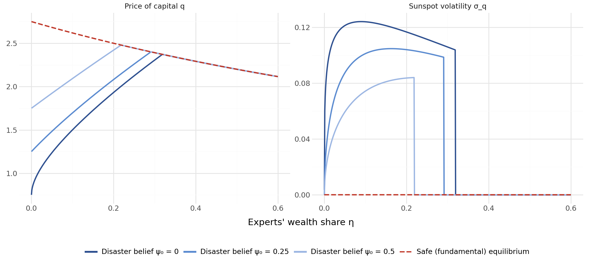
Three features of Figure 43.11 carry the economics. Below a threshold in experts’ wealth share, about one-third under the full fire-sale belief, households hold some of the capital, its price lies below the safe-equilibrium price, and it is volatile even though no fundamental risk is borne by anyone. Volatility is zero when experts are rich enough to absorb the sunspot, jumps up as soon as their wealth share falls below the threshold, and falls back toward zero only when experts are so poor that little capital remains to be sold. And a more optimistic disaster belief shrinks the fire-sale region and lowers volatility throughout, which is the channel through which a credible asset-purchase backstop would work.
The Vietnamese reading starts from the hedging assumption, which is far from local reality. Vietnam has no single-stock futures or options, short selling is effectively unavailable (Table 4.2), and VN30 index futures and covered warrants are the main instruments for transferring equity risk. Most shocks to the balance sheets of leveraged Vietnamese investors are unhedgeable, so the conventional accelerator applies directly. The model’s sharper message is that building out hedging markets would not remove fire-sale fragility. It would move it to the shocks for which no market exists yet, such as the 2022 corporate bond crisis, which hit a market with no instrument for hedging issuer or sector credit risk.
The roles in the model have recognizable counterparts. The “experts” are leveraged holders who value the asset most: margin-financed investors and founders who pledge their own shares as collateral. The “households” are unlevered retail buyers who absorb forced sales at lower valuations. Forced liquidations by securities companies when collateral values fall are the mechanism by which the expert capital share falls with expert wealth. Price limits change the form the fire sale takes. A coordinated sale that drives a stock to its floor, where it locks with an unfilled queue of sell orders, is a discrete jump rather than a smooth decline, which makes the paper’s jump-shock variant the relevant one and links this section to the limit-hit dynamics in Section 38.7.
Four research designs follow.
This chapter developed a comprehensive toolkit for measuring and diagnosing tail risk in Vietnamese equity markets. The key objects estimated (crash risk measures, VaR and Expected Shortfall, tail indices, and tail dependence coefficients) capture distinct but complementary aspects of extreme event behavior.
At the individual stock level, the NCSKEW, DUVOL, and crash count measures quantify asymmetry in firm-specific return distributions, providing forward-looking indicators of crash vulnerability. At the portfolio level, EVT-based approaches to VaR and ES estimation avoid the parametric misspecification that plagues Gaussian and even Student-\(t\) models in the deep tails. At the system level, tail dependence and co-exceedance measures reveal the extent to which crashes propagate across sectors, and the Forbes-Rigobon contagion test distinguishes genuine contagion from the mechanical increase in co-movement driven by higher volatility.
Several features of Vietnamese markets deserve emphasis. Price limits censor the observed return distribution, causing systematic underestimation of true tail risk. The concentration of trading among retail investors amplifies herding-driven crash dynamics. State ownership of large firms creates correlated exposure to policy shocks that is not captured by standard diversification. And the absence of deep derivatives markets limits the hedging instruments available for tail risk management, making accurate measurement all the more critical.
# Tail Risk and Extreme Events
Finance is fundamentally a discipline of extremes. The central objects of concern (e.g., asset pricing, portfolio allocation, capital regulation, systemic stability) are all disproportionately shaped by rare but severe events. A portfolio manager who correctly estimates the mean and variance of returns but ignores the possibility of a $-20\%$ daily move is, in the language of @taleb2010black, "picking up pennies in front of a steamroller." The 1997 Asian Financial Crisis, the 2008 Global Financial Crisis, and the 2020 COVID-19 crash each demonstrated that the most consequential realizations in financial markets are precisely those that conventional Gaussian models assign near-zero probability.
This chapter develops the statistical and econometric toolkit for measuring, modeling, and diagnosing tail risk in Vietnamese equity markets. We focus on three interconnected layers. First, at the individual stock level, we estimate crash risk measures that capture the asymmetry and thickness of the left tail of return distributions. Second, at the portfolio or regulatory level, we implement Value at Risk (VaR) and Expected Shortfall (ES) under multiple estimation approaches and evaluate their accuracy via backtesting. Third, at the system level, we apply Extreme Value Theory (EVT) and tail dependence measures to characterize joint crash behavior across sectors and assess financial contagion.
Vietnamese markets present a particularly rich laboratory for studying tail phenomena. Daily price limits mechanically censor the tails of observed return distributions, creating latent tail risk that is not directly observable but must be inferred. State ownership concentrations, thin liquidity, and herding behavior among retail investors amplify crash dynamics. The absence of a developed derivatives market means that tail hedging instruments familiar in more developed markets (e.g., deep out-of-the-money puts, variance swaps) are largely unavailable, making accurate tail risk measurement all the more important for risk management.
```{python}
#| label: setup
#| message: false
import pandas as pd
import numpy as np
from scipy import stats
from scipy.optimize import minimize
import plotnine as p9
from mizani.formatters import percent_format, comma_format
import warnings
warnings.filterwarnings("ignore")
```
## Crash Risk in Equity Markets
### The Left Tail Problem
The return distribution of individual stocks and market indices is not symmetric. Decades of evidence, beginning with @mandelbrot1963variation and formalized in the asset pricing context by @harvey2000conditional, establish that equity returns exhibit negative skewness (i.e., large negative returns occur more frequently than a Gaussian model predicts) and excess kurtosis (i.e., the tails are thicker than normal in both directions, but the left tail is of primary economic concern).
Let $r_{i,t}$ denote the daily log return of stock $i$ on day $t$. The standardized third central moment (skewness) is:
$$
\text{Skew}(r_i) = \frac{E\left[(r_{i,t} - \mu_i)^3\right]}{\sigma_i^3}
$$ {#eq-skewness}
Negative skewness implies that the distribution has a longer or fatter left tail relative to the right. In economic terms, negative skewness means that large losses are more likely than large gains of equal magnitude. The standardized fourth moment (excess kurtosis) is:
$$
\text{Kurt}(r_i) = \frac{E\left[(r_{i,t} - \mu_i)^4\right]}{\sigma_i^4} - 3
$$ {#eq-kurtosis}
Positive excess kurtosis indicates heavier tails than the normal distribution. Both moments have direct asset pricing implications: @harvey2000conditional and @kraus1976skewness argue that investors demand compensation for holding negatively skewed assets, implying that crash-prone stocks should earn higher expected returns, ceteris paribus.
### Crash Risk Measures
The literature has developed several firm-specific crash risk measures. We implement the three most widely used, following @chen2001forecasting and @hutton2009opaque.
**Measure 1: Negative Coefficient of Skewness (NCSKEW)**
For each firm $i$ in fiscal year $y$, compute firm-specific weekly returns $W_{i,\tau}$ as residuals from a market model augmented with lead and lag market returns to account for nonsynchronous trading:
$$
r_{i,t} = \alpha_i + \beta_{1i} r_{m,t-1} + \beta_{2i} r_{m,t} + \beta_{3i} r_{m,t+1} + \varepsilon_{i,t}
$$ {#eq-crash-model}
where $r_{m,t}$ is the value-weighted market return on day $t$. The firm-specific weekly return is $W_{i,\tau} = \ln(1 + \sum_{t \in \tau} \hat{\varepsilon}_{i,t})$, where $\tau$ indexes weeks. NCSKEW is then:
$$
\text{NCSKEW}_{i,y} = -\frac{n(n-1)^{3/2} \sum W_{i,\tau}^3}{(n-1)(n-2)\left(\sum W_{i,\tau}^2\right)^{3/2}}
$$ {#eq-ncskew}
where $n$ is the number of firm-specific weekly returns in the year. The negative sign ensures that higher NCSKEW corresponds to greater crash risk.
**Measure 2: Down-to-Up Volatility (DUVOL)**
Partition the firm-specific weekly returns into "down weeks" ($W_{i,\tau} < \bar{W}_i$) and "up weeks" ($W_{i,\tau} \geq \bar{W}_i$), where $\bar{W}_i$ is the annual mean. Then:
$$
\text{DUVOL}_{i,y} = \ln\left(\frac{(n_u - 1)\sum_{\text{down}} W_{i,\tau}^2}{(n_d - 1)\sum_{\text{up}} W_{i,\tau}^2}\right)
$$ {#eq-duvol}
where $n_u$ and $n_d$ are the number of up and down weeks, respectively. Higher DUVOL indicates greater crash risk. @chen2001forecasting argue that DUVOL is less sensitive to outliers than NCSKEW because it does not involve the cube of returns.
**Measure 3: Crash Count (COUNT)**
Define a crash event as a firm-specific weekly return that falls below $k$ standard deviations of its annual distribution:
$$
\text{CRASH}_{i,\tau} = \mathbb{1}\left(W_{i,\tau} < \bar{W}_i - k \cdot \hat{\sigma}_{W_i}\right)
$$ {#eq-crash-event}
The standard threshold in the literature is $k = 3.09$, corresponding to the 0.1% tail of a standard normal distribution. The crash count for year $y$ is $\text{COUNT}_{i,y} = \sum_{\tau \in y} \text{CRASH}_{i,\tau}$.
```{python}
#| label: load-data
#| eval: false
# DataCore.vn API
from datacore import DataCore
dc = DataCore()
# Load daily stock returns and market returns
daily_returns = dc.get_daily_returns(
start_date="2010-01-01",
end_date="2024-12-31"
)
# Market return: value-weighted index
market_returns = dc.get_market_returns(
start_date="2010-01-01",
end_date="2024-12-31",
frequency="daily"
)
# Merge
df = daily_returns.merge(
market_returns[["date", "mkt_ret"]],
on="date",
how="left"
)
print(f"Universe: {df['ticker'].nunique()} firms, "
f"{df['date'].nunique()} trading days")
```
```{python}
#| label: firm-specific-returns
#| eval: false
from sklearn.linear_model import LinearRegression
def compute_firm_specific_returns(group):
"""
Estimate firm-specific daily returns from augmented market model
with lead and lag market returns (Chen, Hong, Stein 2001).
"""
g = group.sort_values("date").copy()
g["mkt_lag1"] = g["mkt_ret"].shift(1)
g["mkt_lead1"] = g["mkt_ret"].shift(-1)
g = g.dropna(subset=["ret", "mkt_ret", "mkt_lag1", "mkt_lead1"])
if len(g) < 30:
return pd.DataFrame()
X = g[["mkt_lag1", "mkt_ret", "mkt_lead1"]].values
y = g["ret"].values
model = LinearRegression().fit(X, y)
g["resid"] = y - model.predict(X)
return g[["ticker", "date", "resid"]]
# Estimate by firm-year
df["year"] = df["date"].dt.year
firm_resids = (
df.groupby(["ticker", "year"], group_keys=False)
.apply(compute_firm_specific_returns)
.reset_index(drop=True)
)
```
```{python}
#| label: weekly-aggregation
#| eval: false
# Aggregate daily residuals to weekly firm-specific returns
firm_resids["date"] = pd.to_datetime(firm_resids["date"])
firm_resids["week"] = firm_resids["date"].dt.isocalendar().week.astype(int)
firm_resids["year"] = firm_resids["date"].dt.year
weekly_returns = (
firm_resids.groupby(["ticker", "year", "week"])
.agg(W=("resid", lambda x: np.log(1 + x.sum())))
.reset_index()
)
```
```{python}
#| label: crash-risk-measures
#| eval: false
def compute_crash_measures(group):
"""Compute NCSKEW, DUVOL, and CRASH count for one firm-year."""
W = group["W"].values
n = len(W)
if n < 26: # Require at least 26 weeks
return pd.Series({
"ncskew": np.nan, "duvol": np.nan,
"crash_count": np.nan, "n_weeks": n
})
# NCSKEW
W_demean = W - W.mean()
num = n * (n - 1)**1.5 * np.sum(W_demean**3)
den = (n - 1) * (n - 2) * (np.sum(W_demean**2))**1.5
ncskew = -(num / den) if den != 0 else np.nan
# DUVOL
mean_W = W.mean()
down = W[W < mean_W]
up = W[W >= mean_W]
n_d, n_u = len(down), len(up)
if n_d > 1 and n_u > 1:
duvol = np.log(
((n_u - 1) * np.sum(down**2)) /
((n_d - 1) * np.sum(up**2))
)
else:
duvol = np.nan
# Crash count (k = 3.09)
threshold = W.mean() - 3.09 * W.std()
crash_count = int(np.sum(W < threshold))
return pd.Series({
"ncskew": ncskew,
"duvol": duvol,
"crash_count": crash_count,
"n_weeks": n
})
crash_risk = (
weekly_returns.groupby(["ticker", "year"])
.apply(compute_crash_measures)
.reset_index()
)
crash_risk = crash_risk.dropna(subset=["ncskew", "duvol"])
print(f"Crash risk panel: {len(crash_risk)} firm-years")
```
### Cross-Sectional Distribution of Crash Risk
@tbl-crash-summary presents summary statistics for the three crash risk measures across the Vietnamese equity market.
```{python}
#| label: tbl-crash-summary
#| eval: false
#| tbl-cap: "Summary Statistics of Crash Risk Measures"
summary = crash_risk[["ncskew", "duvol", "crash_count"]].describe(
percentiles=[0.05, 0.25, 0.5, 0.75, 0.95]
).T.round(4)
summary.columns = ["N", "Mean", "Std", "Min", "5%", "25%",
"Median", "75%", "95%", "Max"]
summary
```
```{python}
#| label: fig-ncskew-distribution
#| eval: false
#| fig-cap: "Cross-Sectional Distribution of NCSKEW by Year"
plot_data = crash_risk[crash_risk["year"].between(2012, 2024)].copy()
(
p9.ggplot(plot_data, p9.aes(x="ncskew"))
+ p9.geom_histogram(bins=50, fill="#2E5090", alpha=0.7)
+ p9.facet_wrap("~year", scales="free_y", ncol=4)
+ p9.geom_vline(xintercept=0, linetype="dashed", color="red", size=0.5)
+ p9.labs(
x="NCSKEW",
y="Count",
title="Distribution of Firm-Level Crash Risk (NCSKEW)"
)
+ p9.theme_minimal()
+ p9.theme(figure_size=(12, 8))
)
```
The rightward shift of the NCSKEW distribution during crisis episodes, particularly in 2020 and 2022, indicates a market-wide increase in crash risk. The red dashed line at zero separates firms with negative skewness (right of zero, i.e., high NCSKEW since the measure is negated) from those with positive skewness.
### Interpretation in Asset Pricing
Crash risk has first-order implications for asset pricing. @harvey2000conditional demonstrate that coskewness (i.e., the contribution of an individual asset to the skewness of the aggregate market portfolio) is priced in the cross-section of expected returns. Specifically, assets that tend to crash when the market crashes (negative coskewness) should command a risk premium.
The coskewness of stock $i$ with the market is:
$$
\text{CoSkew}_i = \frac{E\left[(r_i - \mu_i)(r_m - \mu_m)^2\right]}{\sigma_i \cdot \sigma_m^2}
$$ {#eq-coskewness}
Stocks with more negative coskewness exhibit disproportionately poor performance during market downturns. In Vietnam, this is especially relevant because: (1) retail investor herding amplifies co-movement during selloffs; (2) price limits delay crash completion, spreading crash risk across multiple days; and (3) state-owned enterprises, which constitute a large fraction of market capitalization, may exhibit coordinated crash behavior driven by common policy shocks.
```{python}
#| label: coskewness-estimation
#| eval: false
def compute_coskewness(group):
"""Estimate coskewness for a firm-year."""
r_i = group["ret"].values
r_m = group["mkt_ret"].values
if len(r_i) < 60:
return np.nan
r_i_dm = r_i - r_i.mean()
r_m_dm = r_m - r_m.mean()
coskew = (
np.mean(r_i_dm * r_m_dm**2) /
(np.std(r_i) * np.std(r_m)**2)
)
return coskew
df_coskew = (
df.groupby(["ticker", "year"])
.apply(lambda g: pd.Series({"coskewness": compute_coskewness(g)}))
.reset_index()
.dropna()
)
```
```{python}
#| label: fig-coskew-time
#| fig-cap: "Cross-Sectional Median Coskewness Over Time"
#| eval: false
median_coskew = (
df_coskew.groupby("year")
.agg(
median_coskew=("coskewness", "median"),
q25=("coskewness", lambda x: x.quantile(0.25)),
q75=("coskewness", lambda x: x.quantile(0.75))
)
.reset_index()
)
(
p9.ggplot(median_coskew, p9.aes(x="year"))
+ p9.geom_ribbon(
p9.aes(ymin="q25", ymax="q75"),
fill="#2E5090", alpha=0.2
)
+ p9.geom_line(p9.aes(y="median_coskew"), color="#2E5090", size=1)
+ p9.geom_hline(yintercept=0, linetype="dashed", color="gray")
+ p9.labs(
x="Year",
y="Coskewness",
title="Cross-Sectional Coskewness: Median and Interquartile Range"
)
+ p9.theme_minimal()
+ p9.theme(figure_size=(10, 5))
)
```
### Downside Tail Concentration
Beyond skewness, the concentration of returns in the extreme left tail provides additional diagnostic information. We define the downside tail concentration ratio as the fraction of total return variance attributable to observations below the $p$-th percentile:
$$
\text{TCR}_p = \frac{\sum_{r_{i,t} < q_p} (r_{i,t} - \bar{r}_i)^2}{\sum_t (r_{i,t} - \bar{r}_i)^2}
$$ {#eq-tail-concentration}
where $q_p$ is the $p$-th percentile of the firm's return distribution. Under a symmetric distribution, $\text{TCR}_{5\%}$ would be close to $5\%$ (with a slight upward bias due to the squaring). Values substantially exceeding $5\%$ indicate that the left tail contributes disproportionately to total risk.
```{python}
#| label: tail-concentration
#| eval: false
def tail_concentration_ratio(returns, p=0.05):
"""Compute tail concentration ratio at percentile p."""
q = np.quantile(returns, p)
r_dm = returns - returns.mean()
total_var = np.sum(r_dm**2)
tail_var = np.sum(r_dm[returns < q]**2)
return tail_var / total_var if total_var > 0 else np.nan
tcr = (
df.groupby(["ticker", "year"])
.agg(
tcr_5=("ret", lambda x: tail_concentration_ratio(x.values, 0.05)),
tcr_1=("ret", lambda x: tail_concentration_ratio(x.values, 0.01)),
n_obs=("ret", "count")
)
.reset_index()
.query("n_obs >= 120")
)
print("Median TCR(5%):", round(tcr["tcr_5"].median(), 4))
print("Median TCR(1%):", round(tcr["tcr_1"].median(), 4))
```
## Value at Risk and Expected Shortfall
### Definitions
Value at Risk (VaR) and Expected Shortfall (ES) are the two principal quantile-based risk measures used in financial regulation and internal risk management. For a portfolio return $r$ with the cumulative distribution function $F$, the VaR at confidence level $\alpha$ is:
$$
\text{VaR}_\alpha = -F^{-1}(\alpha) = -\inf\{x : F(x) \geq \alpha\}
$$ {#eq-var-def}
This is simply the negative of the $\alpha$-quantile of the return distribution. For $\alpha = 0.01$, $\text{VaR}_{1\%}$ answers: "What is the loss that is exceeded with only 1% probability?"
Expected Shortfall (also called Conditional VaR or CVaR) is the expected loss conditional on the loss exceeding VaR:
$$
\text{ES}_\alpha = -\frac{1}{\alpha}\int_0^\alpha F^{-1}(u) \, du = -E\left[r \mid r \leq -\text{VaR}_\alpha\right]
$$ {#eq-es-def}
For continuous distributions, ES simplifies to the conditional expectation in @eq-es-def. ES is always at least as large as VaR ($\text{ES}_\alpha \geq \text{VaR}_\alpha$) and is strictly larger whenever the distribution has any mass beyond the VaR quantile.
### Why Expected Shortfall Dominates VaR
@tbl-tail-riskvar-vs-es summarizes the fundamental differences.
| Property | VaR | Expected Shortfall |
|-------------------|-------------------|----------------------------------|
| Definition | Quantile of the loss distribution | Conditional mean loss beyond VaR |
| Tail information | None beyond the quantile | Captures severity of tail losses |
| Subadditivity | Not subadditive in general | Subadditive (coherent risk measure) |
| Regulatory status | Basel II primary measure | Basel III/IV primary measure |
| Backtesting | Binary: breach or no breach | Continuous: requires severity assessment |
| Sensitivity to tail shape | None | Directly sensitive |
: Comparison of VaR and Expected Shortfall {#tbl-tail-riskvar-vs-es}
The critical deficiency of VaR is the absence of subadditivity. A risk measure $\rho$ is subadditive if $\rho(X + Y) \leq \rho(X) + \rho(Y)$ for all portfolios $X, Y$. VaR violates this condition for non-elliptical distributions, meaning that diversification can appear to increase risk under VaR, which is a perverse result. @artzner1999coherent established the axiomatic framework for coherent risk measures, and ES satisfies all four axioms: monotonicity, translation invariance, positive homogeneity, and subadditivity. VaR satisfies only three.
### Estimation Methods
We implement four approaches to VaR and ES estimation, each with distinct assumptions and data requirements.
**Method 1: Historical Simulation**
The simplest nonparametric approach uses the empirical distribution directly:
$$
\widehat{\text{VaR}}_\alpha^{\text{HS}} = -\hat{F}_n^{-1}(\alpha) = -r_{(\lceil n\alpha \rceil)}
$$ {#eq-var-hs}
where $r_{(k)}$ is the $k$-th order statistic of the return sample. ES is the average of all returns below the VaR:
$$
\widehat{\text{ES}}_\alpha^{\text{HS}} = -\frac{1}{\lfloor n\alpha \rfloor}\sum_{k=1}^{\lfloor n\alpha \rfloor} r_{(k)}
$$ {#eq-es-hs}
**Method 2: Parametric (Gaussian)**
Assume $r_t \sim N(\mu, \sigma^2)$. Then:
$$
\text{VaR}_\alpha^{\text{Gauss}} = -(\hat{\mu} + \hat{\sigma} \cdot \Phi^{-1}(\alpha))
$$ {#eq-var-gauss}
$$
\text{ES}_\alpha^{\text{Gauss}} = -\hat{\mu} + \hat{\sigma} \cdot \frac{\phi(\Phi^{-1}(\alpha))}{\alpha}
$$ {#eq-es-gauss}
where $\Phi$ and $\phi$ are the standard normal CDF and PDF, respectively. The Gaussian assumption is known to underestimate tail risk for equity returns, but provides a useful baseline.
**Method 3: Parametric (Student-**$t$)
The Student-$t$ distribution with $\nu$ degrees of freedom captures excess kurtosis. The VaR and ES are:
$$
\text{VaR}_\alpha^{t} = -\left(\hat{\mu} + \hat{\sigma}\sqrt{\frac{\nu - 2}{\nu}} \cdot t_\nu^{-1}(\alpha)\right)
$$ {#eq-var-t}
$$
\text{ES}_\alpha^{t} = -\hat{\mu} + \hat{\sigma}\sqrt{\frac{\nu-2}{\nu}} \cdot \frac{f_{t_\nu}(t_\nu^{-1}(\alpha))}{\alpha} \cdot \frac{\nu + (t_\nu^{-1}(\alpha))^2}{\nu - 1}
$$ {#eq-es-t}
where $t_\nu^{-1}$ and $f_{t_\nu}$ are the quantile function and PDF of the Student-$t$ distribution.
**Method 4: GARCH-Filtered EVT (Semi-Parametric)**
This approach, developed by @mcneil2000estimation, first filters returns through a GARCH(1,1) model to obtain standardized residuals $z_t = \hat{\varepsilon}_t / \hat{\sigma}_t$, then fits a Generalized Pareto Distribution (GPD) to the lower tail of the standardized residuals. We detail the EVT component in @sec-evt.
```{python}
#| label: var-es-estimation
#| eval: false
def estimate_var_es(returns, alpha=0.01):
"""
Estimate VaR and ES at level alpha using four methods.
Parameters
----------
returns : array-like
Return series.
alpha : float
Tail probability (e.g., 0.01 for 1%).
Returns
-------
dict : VaR and ES estimates for each method.
"""
r = np.array(returns)
r = r[~np.isnan(r)]
n = len(r)
mu, sigma = r.mean(), r.std(ddof=1)
results = {}
# Method 1: Historical simulation
sorted_r = np.sort(r)
idx = int(np.ceil(n * alpha))
results["var_hs"] = -sorted_r[idx - 1]
results["es_hs"] = -sorted_r[:idx].mean()
# Method 2: Gaussian
z_alpha = stats.norm.ppf(alpha)
results["var_gauss"] = -(mu + sigma * z_alpha)
results["es_gauss"] = -mu + sigma * stats.norm.pdf(z_alpha) / alpha
# Method 3: Student-t (MLE for degrees of freedom)
try:
nu, loc, scale = stats.t.fit(r)
t_alpha = stats.t.ppf(alpha, df=nu)
results["var_t"] = -(loc + scale * t_alpha)
results["es_t"] = (
-loc + scale *
(stats.t.pdf(t_alpha, df=nu) / alpha) *
((nu + t_alpha**2) / (nu - 1))
)
results["nu_hat"] = nu
except Exception:
results["var_t"] = np.nan
results["es_t"] = np.nan
results["nu_hat"] = np.nan
return results
```
```{python}
#| label: market-var-es
#| eval: false
# Compute VaR and ES for the aggregate market index
market_daily = dc.get_market_returns(
start_date="2010-01-01",
end_date="2024-12-31",
frequency="daily"
)
# Rolling 1-year VaR/ES
window = 252
results_list = []
for end_idx in range(window, len(market_daily)):
window_returns = market_daily["mkt_ret"].iloc[end_idx - window:end_idx].values
date = market_daily["date"].iloc[end_idx]
est = estimate_var_es(window_returns, alpha=0.01)
est["date"] = date
results_list.append(est)
var_es_ts = pd.DataFrame(results_list)
```
```{python}
#| label: fig-var-comparison
#| eval: false
#| fig-cap: "Rolling 1% VaR Estimates: Historical, Gaussian, and Student-t Methods"
plot_var = var_es_ts.melt(
id_vars="date",
value_vars=["var_hs", "var_gauss", "var_t"],
var_name="method",
value_name="var"
)
method_labels = {
"var_hs": "Historical Simulation",
"var_gauss": "Gaussian",
"var_t": "Student-t"
}
plot_var["method"] = plot_var["method"].map(method_labels)
(
p9.ggplot(plot_var, p9.aes(x="date", y="var", color="method"))
+ p9.geom_line(alpha=0.8, size=0.6)
+ p9.labs(
x="", y="1% VaR (Loss)",
title="Rolling 252-Day Value at Risk Estimates",
color="Method"
)
+ p9.scale_color_manual(
values=["#2E5090", "#C0392B", "#27AE60"]
)
+ p9.theme_minimal()
+ p9.theme(figure_size=(12, 5), legend_position="top")
)
```
```{python}
#| label: fig-es-comparison
#| eval: false
#| fig-cap: "Rolling 1% Expected Shortfall Estimates"
plot_es = var_es_ts.melt(
id_vars="date",
value_vars=["es_hs", "es_gauss", "es_t"],
var_name="method",
value_name="es"
)
method_labels_es = {
"es_hs": "Historical Simulation",
"es_gauss": "Gaussian",
"es_t": "Student-t"
}
plot_es["method"] = plot_es["method"].map(method_labels_es)
(
p9.ggplot(plot_es, p9.aes(x="date", y="es", color="method"))
+ p9.geom_line(alpha=0.8, size=0.6)
+ p9.labs(
x="", y="1% ES (Loss)",
title="Rolling 252-Day Expected Shortfall Estimates",
color="Method"
)
+ p9.scale_color_manual(
values=["#2E5090", "#C0392B", "#27AE60"]
)
+ p9.theme_minimal()
+ p9.theme(figure_size=(12, 5), legend_position="top")
)
```
### VaR Backtesting
A VaR model is only useful if its predictions are accurate. Backtesting evaluates whether the realized frequency of VaR breaches is consistent with the nominal confidence level. If VaR is estimated at the $\alpha = 1\%$ level, we expect approximately 1% of days to exhibit losses exceeding VaR.
The Kupiec unconditional coverage test [@kupiec1995techniques] evaluates whether the total number of breaches $x$ in $n$ observations is consistent with $\alpha$:
$$
\text{LR}_{\text{UC}} = -2\ln\left(\frac{\alpha^x (1-\alpha)^{n-x}}{\hat{p}^x (1-\hat{p})^{n-x}}\right) \sim \chi^2(1)
$$ {#eq-kupiec}
where $\hat{p} = x/n$ is the empirical breach frequency. The Christoffersen conditional coverage test [@christoffersen1998evaluating] additionally evaluates whether breaches are independent (no clustering):
$$
\text{LR}_{\text{CC}} = \text{LR}_{\text{UC}} + \text{LR}_{\text{IND}}
$$ {#eq-christoffersen}
where $\text{LR}_{\text{IND}}$ tests the null of independence using a first-order Markov chain model for breach indicators.
```{python}
#| label: backtesting
#| eval: false
def kupiec_test(returns, var_estimates, alpha=0.01):
"""
Kupiec unconditional coverage test for VaR backtesting.
Returns
-------
dict : breach count, expected, breach rate, LR statistic, p-value.
"""
breaches = returns < -var_estimates
x = breaches.sum()
n = len(returns)
p_hat = x / n
if p_hat == 0 or p_hat == 1:
return {"breaches": x, "expected": n * alpha,
"breach_rate": p_hat, "lr_stat": np.nan, "p_value": np.nan}
lr = -2 * (
x * np.log(alpha) + (n - x) * np.log(1 - alpha)
- x * np.log(p_hat) - (n - x) * np.log(1 - p_hat)
)
p_value = 1 - stats.chi2.cdf(lr, df=1)
return {
"breaches": int(x),
"expected": round(n * alpha, 1),
"breach_rate": round(p_hat, 4),
"lr_stat": round(lr, 4),
"p_value": round(p_value, 4)
}
# Backtest each method
actual_returns = market_daily["mkt_ret"].iloc[window:].values
backtest_results = {}
for method, col in [("Historical", "var_hs"),
("Gaussian", "var_gauss"),
("Student-t", "var_t")]:
backtest_results[method] = kupiec_test(
actual_returns, var_es_ts[col].values, alpha=0.01
)
bt_df = pd.DataFrame(backtest_results).T
bt_df.index.name = "Method"
bt_df
```
### Estimation Under Limited Data {#sec-limited-data}
In Vietnamese equity markets, many stocks have short trading histories, thin liquidity, and censored returns due to price limits. These features create challenges for tail risk estimation that are less severe in developed markets.
**Price limit censoring.** When a stock hits its daily price limit, the observed return is truncated. The true latent return may extend well beyond the limit, but is unobservable. This means that historical simulation mechanically understates VaR and ES for stocks that frequently hit limits. A Tobit-type correction can partially address this:
$$
r_{i,t}^{\text{latent}} \sim N(\mu_i, \sigma_i^2), \quad r_{i,t}^{\text{obs}} = \max(\underline{L}, \min(\bar{L}, r_{i,t}^{\text{latent}}))
$$ {#eq-tobit-var}
The parameters $(\mu_i, \sigma_i^2)$ can be estimated via maximum likelihood on the censored sample, and VaR/ES can then be computed from the estimated latent distribution.
**Short histories.** For recently listed stocks, the available sample may be too short for reliable nonparametric estimation. In these cases, shrinkage toward a cross-sectional prior (e.g., the sector median VaR) or Bayesian approaches with informative priors can improve stability.
## Extreme Value Theory {#sec-evt}
### Motivation: What EVT Captures That GARCH Does Not
GARCH models capture volatility clustering (i.e., the tendency of large returns to be followed by large returns), but they make specific distributional assumptions about standardized residuals (typically Gaussian or Student-$t$). The tail behavior of the conditional distribution is thus determined by the parametric innovation assumption, not learned from the data.
Extreme Value Theory (EVT) takes a fundamentally different approach. It provides a statistical framework for estimating the distribution of extreme observations without specifying the entire return distribution. The key theoretical results (i.e., the Fisher-Tippett-Gnedenko theorem and the Pickands-Balkema-de Haan theorem) establish that the distribution of properly normalized maxima (or exceedances over high thresholds) converges to specific parametric families regardless of the parent distribution. This universality is what makes EVT powerful: the tail can be estimated even when the center of the distribution is misspecified.
### Tail Index Estimation
The tail index $\xi$ (also denoted $\alpha^{-1}$ in some formulations) governs the rate of tail decay. For heavy-tailed distributions, the survival function satisfies:
$$
P(X > x) \sim L(x) \cdot x^{-1/\xi}, \quad x \to \infty
$$ {#eq-tail-decay}
where $L(x)$ is a slowly varying function. The tail index $\xi > 0$ implies a Pareto-type tail; larger $\xi$ means heavier tails. Financial return distributions typically have $\xi \in (0.2, 0.5)$, corresponding to tail indices $\alpha = 1/\xi \in (2, 5)$, which implies finite variance but potentially infinite higher moments.
The Hill estimator [@hill1975simple] provides a simple nonparametric estimate of $\xi$ from the upper order statistics:
$$
\hat{\xi}_{\text{Hill}}(k) = \frac{1}{k}\sum_{j=1}^{k} \ln X_{(n-j+1)} - \ln X_{(n-k)}
$$ {#eq-hill}
where $X_{(1)} \leq \cdots \leq X_{(n)}$ are the order statistics and $k$ is the number of upper order statistics used. The choice of $k$ involves a bias-variance tradeoff: small $k$ yields high variance; large $k$ introduces bias from non-tail observations.
```{python}
#| label: hill-estimator
#| eval: false
def hill_estimator(data, k_values=None):
"""
Compute Hill estimator of tail index for a range of k values.
Parameters
----------
data : array-like
Positive values (use absolute values of losses).
k_values : array-like, optional
Number of upper order statistics to use.
Returns
-------
DataFrame with columns [k, xi_hat, se].
"""
x = np.sort(np.abs(data))[::-1] # Descending order
n = len(x)
if k_values is None:
k_values = range(10, min(n // 2, 500), 5)
results = []
for k in k_values:
if k >= n or k < 2:
continue
log_excess = np.log(x[:k]) - np.log(x[k])
xi_hat = log_excess.mean()
se = xi_hat / np.sqrt(k)
results.append({"k": k, "xi_hat": xi_hat, "se": se})
return pd.DataFrame(results)
```
```{python}
#| label: fig-hill-plot
#| eval: false
#| fig-cap: "Hill Plot: Tail Index Estimate as a Function of Order Statistics"
# Use negative market returns (losses)
losses = -market_daily["mkt_ret"].dropna().values
losses_positive = losses[losses > 0]
hill_results = hill_estimator(losses_positive)
(
p9.ggplot(hill_results, p9.aes(x="k", y="xi_hat"))
+ p9.geom_ribbon(
p9.aes(ymin="xi_hat - 1.96 * se", ymax="xi_hat + 1.96 * se"),
fill="#2E5090", alpha=0.2
)
+ p9.geom_line(color="#2E5090", size=0.8)
+ p9.geom_hline(yintercept=0.33, linetype="dashed", color="red")
+ p9.annotate(
"text", x=hill_results["k"].max() * 0.7, y=0.35,
label="ξ = 1/3 (cubic tail)", color="red", size=8
)
+ p9.labs(
x="Number of Order Statistics (k)",
y="Hill Estimate ξ̂",
title="Hill Plot for Market Return Left Tail"
)
+ p9.theme_minimal()
+ p9.theme(figure_size=(10, 5))
)
```
The Hill plot is a standard diagnostic in EVT. A stable region of the Hill estimate across a range of $k$ suggests a reliable tail index estimate. The red dashed line at $\xi = 1/3$ corresponds to a tail index of $\alpha = 3$, which implies that the third moment (skewness) is infinite, which is a finding consistent with much of the empirical finance literature [@cont2001empirical; @gabaix2003theory].
### Block Maxima and the GEV Distribution
The Fisher-Tippett-Gnedenko theorem establishes that if the maximum of $n$ i.i.d. random variables, after proper normalization, converges in distribution, the limit must be a Generalized Extreme Value (GEV) distribution:
$$
G_\xi(x) = \exp\left\{-\left(1 + \xi \cdot \frac{x - \mu}{\sigma}\right)^{-1/\xi}\right\}
$$ {#eq-gev}
for $1 + \xi(x - \mu)/\sigma > 0$, where $\mu$ is the location, $\sigma > 0$ the scale, and $\xi$ the shape parameter. The three sub-families are in @tbl-tail-riskgev-families.
| Shape $\xi$ | Distribution | Tail Type | Finance Example |
|------------------|------------------|------------------|-------------------|
| $\xi > 0$ | Fréchet | Heavy (polynomial decay) | Equity returns, credit losses |
| $\xi = 0$ | Gumbel | Light (exponential decay) | Normal/lognormal models |
| $\xi < 0$ | Weibull | Bounded upper tail | Bounded loss distributions |
: GEV Sub-Families and Financial Interpretation {#tbl-tail-riskgev-families}
For the block maxima approach, we divide the return series into non-overlapping blocks (typically months or quarters) and extract the minimum return (maximum loss) from each block. The GEV is then fitted to these block minima.
```{python}
#| label: block-maxima
#| eval: false
from scipy.stats import genextreme
# Monthly block minima (maximum losses)
market_daily["month"] = market_daily["date"].dt.to_period("M")
block_minima = (
market_daily.groupby("month")
.agg(min_ret=("mkt_ret", "min"))
.reset_index()
)
# Fit GEV to negated block minima (so we model maxima of losses)
block_losses = -block_minima["min_ret"].values
xi_hat, loc_hat, scale_hat = genextreme.fit(block_losses)
print(f"GEV fit to monthly block maxima of losses:")
print(f" Shape (ξ): {xi_hat:.4f}")
print(f" Location (μ): {loc_hat:.4f}")
print(f" Scale (σ): {scale_hat:.4f}")
```
```{python}
#| label: fig-gev-fit
#| eval: false
#| fig-cap: "GEV Fit to Monthly Maximum Losses"
x_grid = np.linspace(
block_losses.min() * 0.8,
block_losses.max() * 1.2,
200
)
gev_pdf = genextreme.pdf(x_grid, xi_hat, loc=loc_hat, scale=scale_hat)
plot_data = pd.DataFrame({
"x": np.concatenate([block_losses, x_grid]),
"source": (["Empirical"] * len(block_losses) +
["GEV Fit"] * len(x_grid)),
"density": np.concatenate([
np.full(len(block_losses), np.nan),
gev_pdf
]),
"value": np.concatenate([block_losses, np.full(len(x_grid), np.nan)])
})
empirical = plot_data[plot_data["source"] == "Empirical"]
fitted = plot_data[plot_data["source"] == "GEV Fit"]
(
p9.ggplot()
+ p9.geom_histogram(
data=empirical, mapping=p9.aes(x="value", y="..density.."),
bins=30, fill="#2E5090", alpha=0.5
)
+ p9.geom_line(
data=fitted, mapping=p9.aes(x="x", y="density"),
color="#C0392B", size=1
)
+ p9.labs(
x="Monthly Maximum Loss",
y="Density",
title="GEV Distribution Fit to Monthly Block Maxima"
)
+ p9.theme_minimal()
+ p9.theme(figure_size=(10, 5))
)
```
### Peaks Over Threshold and the GPD {#sec-gpd}
The Peaks Over Threshold (POT) approach is generally preferred over block maxima because it uses tail data more efficiently. The Pickands-Balkema-de Haan theorem establishes that for a sufficiently high threshold $u$, the distribution of exceedances $Y = X - u \mid X > u$ converges to a Generalized Pareto Distribution (GPD):
$$
H_{\xi,\beta}(y) = \begin{cases}
1 - \left(1 + \frac{\xi y}{\beta}\right)^{-1/\xi} & \text{if } \xi \neq 0 \\
1 - \exp\left(-\frac{y}{\beta}\right) & \text{if } \xi = 0
\end{cases}
$$ {#eq-gpd}
for $y > 0$ and $1 + \xi y / \beta > 0$, where $\beta > 0$ is the scale parameter and $\xi$ is the shape parameter (identical to the GEV shape). The POT-based VaR and ES at level $\alpha$ are:
$$
\text{VaR}_\alpha^{\text{GPD}} = u + \frac{\hat{\beta}}{\hat{\xi}}\left[\left(\frac{n}{N_u} \cdot \alpha\right)^{-\hat{\xi}} - 1\right]
$$ {#eq-var-gpd}
$$
\text{ES}_\alpha^{\text{GPD}} = \frac{\text{VaR}_\alpha^{\text{GPD}}}{1 - \hat{\xi}} + \frac{\hat{\beta} - \hat{\xi} u}{1 - \hat{\xi}}
$$ {#eq-es-gpd}
where $N_u$ is the number of observations exceeding $u$ and $n$ is the total sample size. These formulae are valid for $\hat{\xi} < 1$.
```{python}
#| label: gpd-estimation
#| eval: false
from scipy.stats import genpareto
def fit_gpd_pot(returns, threshold_quantile=0.95):
"""
Fit GPD to exceedances over threshold using POT approach.
Parameters
----------
returns : array-like
Return series (losses should be positive).
threshold_quantile : float
Quantile for threshold selection.
Returns
-------
dict : Threshold, GPD parameters, VaR, ES estimates.
"""
losses = -np.array(returns)
losses = losses[~np.isnan(losses)]
n = len(losses)
u = np.quantile(losses, threshold_quantile)
exceedances = losses[losses > u] - u
N_u = len(exceedances)
# Fit GPD
xi_hat, _, beta_hat = genpareto.fit(exceedances, floc=0)
# VaR and ES at 1%
alpha = 0.01
var_gpd = u + (beta_hat / xi_hat) * (
(n / N_u * alpha)**(-xi_hat) - 1
)
es_gpd = var_gpd / (1 - xi_hat) + (beta_hat - xi_hat * u) / (1 - xi_hat)
return {
"threshold": u,
"n_exceedances": N_u,
"xi_hat": xi_hat,
"beta_hat": beta_hat,
"var_1pct": var_gpd,
"es_1pct": es_gpd
}
# Fit GPD to market losses
gpd_results = fit_gpd_pot(market_daily["mkt_ret"].dropna().values, 0.95)
print("GPD-POT Results (1% level):")
for k, v in gpd_results.items():
if isinstance(v, float):
print(f" {k}: {v:.6f}")
else:
print(f" {k}: {v}")
```
### Threshold Selection
The choice of threshold $u$ is the key practical decision in POT analysis. Too low a threshold violates the asymptotic approximation; too high wastes data. The mean residual life plot provides a graphical diagnostic: if the GPD approximation holds above $u_0$, the mean excess function $e(u) = E[X - u \mid X > u]$ is linear in $u$ for $u > u_0$:
$$
e(u) = \frac{\beta + \xi u}{1 - \xi}
$$ {#eq-mean-excess}
```{python}
#| label: fig-mean-residual-life
#| eval: false
#| fig-cap: "Mean Residual Life Plot for Threshold Selection"
losses = -market_daily["mkt_ret"].dropna().values
losses_sorted = np.sort(losses)
thresholds = np.quantile(losses, np.linspace(0.80, 0.99, 50))
mean_excess = []
for u in thresholds:
exceedances = losses[losses > u] - u
if len(exceedances) > 5:
mean_excess.append({
"threshold": u,
"mean_excess": exceedances.mean(),
"se": exceedances.std() / np.sqrt(len(exceedances)),
"n_exceed": len(exceedances)
})
mrl_df = pd.DataFrame(mean_excess)
(
p9.ggplot(mrl_df, p9.aes(x="threshold", y="mean_excess"))
+ p9.geom_ribbon(
p9.aes(
ymin="mean_excess - 1.96 * se",
ymax="mean_excess + 1.96 * se"
),
fill="#2E5090", alpha=0.2
)
+ p9.geom_line(color="#2E5090", size=0.8)
+ p9.geom_point(color="#2E5090", size=1.5)
+ p9.labs(
x="Threshold (u)",
y="Mean Excess e(u)",
title="Mean Residual Life Plot"
)
+ p9.theme_minimal()
+ p9.theme(figure_size=(10, 5))
)
```
A threshold in the region where the mean residual life plot is approximately linear is appropriate. In practice, we also compare GPD parameter stability across a range of thresholds and select the lowest threshold at which estimates stabilize.
### What EVT Captures That GARCH Does Not
@tbl-tail-riskevt-vs-garch summarizes the complementary roles of these two modeling frameworks.
| Feature | GARCH | EVT |
|-----------------------------|------------------------|-------------------|
| What is modeled | Conditional variance dynamics | Unconditional tail distribution |
| Distributional assumption | Full distribution (Gaussian or $t$) | Only the tail (GPD or GEV) |
| Time dependence | Explicit (volatility clustering) | None (i.i.d. or filtered) |
| Tail shape | Determined by innovation distribution | Estimated from data |
| Extreme quantiles | Extrapolation from parametric assumption | Principled extrapolation via EVT theorems |
| Best use | Short-horizon risk forecasting | Extreme quantile estimation, stress testing |
: GARCH vs. EVT: Complementary Frameworks {#tbl-tail-riskevt-vs-garch}
The GARCH-filtered EVT approach of @mcneil2000estimation combines both: GARCH captures the time-varying volatility, and EVT models the residual tail. This hybrid approach is considered best practice for financial risk management [@mcneil2015quantitative].
## Tail Dependence and Contagion
### Why Correlation Breaks Down in Crises
Perhaps the most important practical fact about multivariate tail risk is that correlations estimated from the body of the distribution systematically understate dependence in the tails. @longin2001extreme demonstrate this using extreme value theory: for bivariate normal returns, the correlation of extreme realizations converges to zero as the threshold moves further into the tail. Yet empirically, the correlation of crash returns remains large and often increases (a phenomenon incompatible with multivariate normality).
Formally, the coefficient of lower tail dependence between two return series $X$ and $Y$ is:
$$
\lambda_L = \lim_{q \to 0^+} P\left(Y \leq F_Y^{-1}(q) \mid X \leq F_X^{-1}(q)\right)
$$ {#eq-tail-dependence}
If $\lambda_L > 0$, the two series exhibit asymptotic tail dependence (i.e., extreme losses tend to occur jointly). For the bivariate normal distribution, $\lambda_L = 0$ for all $|\rho| < 1$ (asymptotic tail independence). This means that any model built on multivariate normality will structurally underestimate the probability of joint crashes. The Student-$t$ copula, by contrast, has $\lambda_L > 0$ for $\rho > -1$, which is why it has become the workhorse model for joint tail risk in finance [@demarta2005t].
### Co-Crash Measures
We implement several empirical measures of joint crash behavior.
**Exceedance Correlation.** Following @longin2001extreme, compute the correlation of returns conditional on both returns falling below a threshold $\theta$:
$$
\rho^-(\theta) = \text{Corr}(r_i, r_j \mid r_i < \theta, r_j < \theta)
$$ {#eq-exceedance-corr}
If returns are bivariate normal, $\rho^-(\theta) \to 0$ as $\theta \to -\infty$. Empirically, $\rho^-(\theta)$ typically increases as $\theta$ decreases, indicating tail dependence beyond what the normal model implies.
**Co-Exceedance Count.** For each day $t$, count the number of stocks or sectors whose returns fall below the $q$-th percentile of their respective marginal distributions:
$$
C_t(q) = \sum_{i=1}^{N} \mathbb{1}\left(r_{i,t} < F_i^{-1}(q)\right)
$$ {#eq-coexceedance}
Days with high $C_t(q)$ represent system-wide stress events.
```{python}
#| label: tail-dependence-estimation
#| eval: false
def empirical_tail_dependence(x, y, quantiles=None):
"""
Estimate lower tail dependence coefficient at various quantiles.
Uses the empirical copula approach: transform to uniform margins,
then estimate P(V <= q | U <= q) for decreasing q.
"""
if quantiles is None:
quantiles = [0.20, 0.15, 0.10, 0.05, 0.03, 0.01]
# Transform to uniform margins via empirical CDF
from scipy.stats import rankdata
n = len(x)
u = rankdata(x) / (n + 1)
v = rankdata(y) / (n + 1)
results = []
for q in quantiles:
mask_u = u <= q
mask_both = mask_u & (v <= q)
n_u = mask_u.sum()
n_both = mask_both.sum()
lambda_hat = n_both / n_u if n_u > 0 else np.nan
results.append({
"quantile": q,
"lambda_L": lambda_hat,
"n_below_x": int(n_u),
"n_co_crash": int(n_both)
})
return pd.DataFrame(results)
```
```{python}
#| label: sector-tail-dependence
#| eval: false
# Load sector-level daily returns
sector_returns = dc.get_sector_returns(
start_date="2010-01-01",
end_date="2024-12-31",
frequency="daily"
)
# Compute pairwise tail dependence for major sectors
sectors = sector_returns["sector"].unique()[:8] # Top 8 sectors
import itertools
pairwise_td = []
for s1, s2 in itertools.combinations(sectors, 2):
r1 = sector_returns.loc[
sector_returns["sector"] == s1, ["date", "ret"]
].set_index("date")["ret"]
r2 = sector_returns.loc[
sector_returns["sector"] == s2, ["date", "ret"]
].set_index("date")["ret"]
# Align dates
aligned = pd.concat([r1, r2], axis=1, join="inner").dropna()
if len(aligned) < 500:
continue
td = empirical_tail_dependence(
aligned.iloc[:, 0].values,
aligned.iloc[:, 1].values,
quantiles=[0.05]
)
pairwise_td.append({
"sector_1": s1,
"sector_2": s2,
"lambda_L_5pct": td["lambda_L"].iloc[0],
"pearson_corr": aligned.iloc[:, 0].corr(aligned.iloc[:, 1])
})
td_df = pd.DataFrame(pairwise_td)
```
```{python}
#| label: tbl-tail-dependence
#| eval: false
#| tbl-cap: "Pairwise Tail Dependence vs. Linear Correlation Across Sectors"
td_display = td_df.copy()
td_display["lambda_L_5pct"] = td_display["lambda_L_5pct"].round(4)
td_display["pearson_corr"] = td_display["pearson_corr"].round(4)
td_display["ratio"] = (
td_display["lambda_L_5pct"] / td_display["pearson_corr"]
).round(3)
td_display.sort_values("lambda_L_5pct", ascending=False).head(15)
```
The ratio column in @tbl-tail-dependence is particularly informative. When $\lambda_L / \rho \gg 1$, the sectors exhibit disproportionately high co-crash frequency relative to their overall correlation. This is the hallmark of tail dependence that Gaussian models miss.
### System-Wide Stress Transmission
To assess system-wide contagion dynamics, we construct daily co-exceedance counts and examine their time-series properties.
```{python}
#| label: coexceedance
#| eval: false
# Compute daily co-exceedance count at the 5% level
sector_wide = sector_returns.pivot_table(
index="date", columns="sector", values="ret"
)
# Rolling 252-day quantile thresholds
quantile_thresholds = sector_wide.rolling(252, min_periods=60).quantile(0.05)
# Indicator: return below rolling 5th percentile
exceedance_indicators = (sector_wide < quantile_thresholds).astype(int)
co_exceedance = exceedance_indicators.sum(axis=1)
co_exceedance.name = "co_exceedance"
co_exceed_df = co_exceedance.reset_index()
co_exceed_df.columns = ["date", "co_exceedance"]
co_exceed_df["n_sectors"] = exceedance_indicators.notna().sum(axis=1).values
```
```{python}
#| label: fig-coexceedance-ts
#| eval: false
#| fig-cap: "Daily Co-Exceedance Count: Number of Sectors Below Their 5th Percentile"
(
p9.ggplot(co_exceed_df.dropna(), p9.aes(x="date", y="co_exceedance"))
+ p9.geom_line(color="#2E5090", alpha=0.5, size=0.3)
+ p9.geom_smooth(method="lowess", color="#C0392B", size=1, se=False)
+ p9.labs(
x="",
y="Number of Sectors in Left Tail",
title="System-Wide Stress: Daily Co-Exceedance Count"
)
+ p9.theme_minimal()
+ p9.theme(figure_size=(12, 5))
)
```
Peaks in the co-exceedance series correspond to system-wide stress episodes. The smoothed trend (red line) reveals the evolving baseline level of systemic fragility.
### Financial Contagion Mechanisms
The literature distinguishes several channels through which stress propagates across assets, sectors, and markets [@forbes2002no; @kaminsky2002unholy]:
**Direct linkages.** Balance sheet interconnections, interbank lending, and cross-holdings create direct transmission channels. When institution $A$ holds assets issued by institution $B$, losses at $B$ directly impair $A$'s balance sheet.
**Information contagion.** Adverse news about one firm triggers reassessment of similarly exposed firms. @king1990transmission and @kodres2002rational formalize this via Bayesian updating: investors cannot distinguish idiosyncratic from systematic shocks, so a crash in one asset leads them to update beliefs about common risk factors.
**Liquidity contagion.** Fire sales by distressed institutions depress prices of commonly held assets, creating losses for other holders. @brunnermeier2009deciphering model this as a liquidity spiral: declining prices trigger margin calls, which force further sales, further depressing prices. In Vietnamese markets, the absence of circuit breakers beyond price limits and the concentration of holdings among a few large institutional investors amplify this channel.
**Behavioral contagion.** Herding behavior (i.e., investors mimicking others' trades) generates correlated selling pressure even in the absence of fundamental linkages. @bikhchandani1992theory and @banerjee1992simple provide theoretical foundations. @choe2005domestic document herding in emerging markets specifically.
We can test for contagion (as distinct from interdependence) using the @forbes2002no framework. The null hypothesis is that the co-movement observed during a crisis period is fully explained by the increase in volatility (which mechanically inflates correlations). The adjusted correlation is:
$$
\rho^* = \frac{\rho_{\text{crisis}}}{\sqrt{1 + \delta[1 - \rho_{\text{crisis}}^2]}}
$$ {#eq-forbes-rigobon}
where $\delta = \sigma_{\text{crisis}}^2 / \sigma_{\text{tranquil}}^2 - 1$ is the relative increase in variance. If $\rho^* > \rho_{\text{tranquil}}$, the increase in co-movement exceeds what volatility adjustment alone predicts, which is evidence of contagion.
```{python}
#| label: contagion-test
#| eval: false
def forbes_rigobon_test(returns_df, crisis_start, crisis_end):
"""
Forbes-Rigobon adjusted correlation test for contagion.
Parameters
----------
returns_df : DataFrame
Columns are sector returns, index is date.
crisis_start, crisis_end : str
Crisis period boundaries.
Returns
-------
DataFrame : Pairwise contagion test results.
"""
tranquil = returns_df[returns_df.index < crisis_start].dropna()
crisis = returns_df[
(returns_df.index >= crisis_start) &
(returns_df.index <= crisis_end)
].dropna()
sectors = returns_df.columns.tolist()
results = []
for s1, s2 in itertools.combinations(sectors, 2):
if s1 not in tranquil.columns or s2 not in crisis.columns:
continue
rho_t = tranquil[s1].corr(tranquil[s2])
rho_c = crisis[s1].corr(crisis[s2])
var_t = tranquil[s1].var()
var_c = crisis[s1].var()
if var_t == 0:
continue
delta = var_c / var_t - 1
rho_adj = rho_c / np.sqrt(1 + delta * (1 - rho_c**2))
results.append({
"sector_1": s1,
"sector_2": s2,
"rho_tranquil": round(rho_t, 4),
"rho_crisis": round(rho_c, 4),
"rho_adjusted": round(rho_adj, 4),
"contagion": rho_adj > rho_t
})
return pd.DataFrame(results)
```
```{python}
#| label: contagion-covid
#| eval: false
# Test for contagion during COVID-19 crash
contagion_covid = forbes_rigobon_test(
sector_wide,
crisis_start="2020-02-01",
crisis_end="2020-04-30"
)
n_pairs = len(contagion_covid)
n_contagion = contagion_covid["contagion"].sum()
print(f"COVID-19 contagion test: {n_contagion}/{n_pairs} sector pairs "
f"show evidence of contagion ({100*n_contagion/n_pairs:.1f}%)")
```
```{python}
#| label: tbl-contagion-results
#| eval: false
#| tbl-cap: "Forbes-Rigobon Contagion Test: COVID-19 Crisis Period"
contagion_covid.sort_values(
"rho_adjusted", ascending=False
).head(15)
```
## Applications to Financial Stability
### Market-Wide Stress Indicators
We construct several market-wide stress indicators that aggregate the individual-level and sectoral tail risk measures developed above into a comprehensive system-level diagnostic.
**Aggregate Crash Risk Index.** The cross-sectional average of firm-level NCSKEW provides a market-wide measure of crash risk that is forward-looking (it captures the buildup of negative skewness before a crash materializes):
$$
\text{ACRI}_y = \frac{1}{N_y}\sum_{i=1}^{N_y} \text{NCSKEW}_{i,y}
$$ {#eq-acri}
**Market Tail Risk (MTR).** Following @kelly2014tail, we estimate the time-varying tail risk of the market portfolio using option-implied or realized tail measures. In the absence of a liquid options market in Vietnam, we use the realized version based on the Hill tail index estimated from rolling windows:
$$
\text{MTR}_t = \hat{\xi}_t^{\text{Hill}} \cdot \hat{\sigma}_t
$$ {#eq-mtr}
where $\hat{\xi}_t^{\text{Hill}}$ is the Hill estimator computed from a trailing 252-day window and $\hat{\sigma}_t$ is the conditional volatility (e.g., from GARCH). This interaction captures both the thickness of the tail and the current scale of volatility.
```{python}
#| label: stability-indicators
#| eval: false
# Aggregate Crash Risk Index
acri = (
crash_risk.groupby("year")
.agg(
acri=("ncskew", "mean"),
median_ncskew=("ncskew", "median"),
pct_high_crash=("ncskew", lambda x: (x > x.quantile(0.75)).mean()),
n_firms=("ncskew", "count")
)
.reset_index()
)
# Market Tail Risk: rolling Hill estimator x rolling volatility
mkt_returns = market_daily["mkt_ret"].dropna().values
dates = market_daily["date"].dropna().values
mtr_list = []
for end_idx in range(504, len(mkt_returns)):
window_ret = mkt_returns[end_idx - 252:end_idx]
losses_pos = -window_ret[window_ret < 0]
if len(losses_pos) < 30:
continue
# Hill estimator at k = 50
sorted_losses = np.sort(losses_pos)[::-1]
k = min(50, len(sorted_losses) - 1)
if k < 10:
continue
log_excess = np.log(sorted_losses[:k]) - np.log(sorted_losses[k])
xi_hat = log_excess.mean()
sigma_hat = window_ret.std()
mtr = xi_hat * sigma_hat
mtr_list.append({
"date": dates[end_idx],
"xi_hat": xi_hat,
"sigma_hat": sigma_hat,
"mtr": mtr
})
mtr_df = pd.DataFrame(mtr_list)
mtr_df["date"] = pd.to_datetime(mtr_df["date"])
```
```{python}
#| label: fig-stability-dashboard
#| eval: false
#| fig-cap: "Market Tail Risk Indicator Over Time"
(
p9.ggplot(mtr_df, p9.aes(x="date", y="mtr"))
+ p9.geom_line(color="#2E5090", alpha=0.5, size=0.4)
+ p9.geom_smooth(method="lowess", color="#C0392B", size=1, se=False)
+ p9.labs(
x="",
y="MTR (ξ × σ)",
title="Market Tail Risk: Rolling Hill Index × Conditional Volatility"
)
+ p9.theme_minimal()
+ p9.theme(figure_size=(12, 5))
)
```
### Sectoral Fragility
Not all sectors are equally vulnerable to tail events. We decompose system-wide tail risk into sectoral contributions to identify the most fragile parts of the market.
```{python}
#| label: sectoral-fragility
#| eval: false
# Sector-level tail statistics
sector_tail_stats = []
for sector in sectors:
sector_data = sector_returns[sector_returns["sector"] == sector]["ret"].dropna()
if len(sector_data) < 500:
continue
s_data = sector_data.values
# Skewness and kurtosis
skew = stats.skew(s_data)
kurt = stats.kurtosis(s_data)
# VaR and ES at 1%
var_1 = -np.quantile(s_data, 0.01)
es_1 = -s_data[s_data <= np.quantile(s_data, 0.01)].mean()
# Hill tail index (k=50)
losses_pos = -s_data[s_data < 0]
sorted_l = np.sort(losses_pos)[::-1]
k = min(50, len(sorted_l) - 1)
if k >= 10:
log_exc = np.log(sorted_l[:k]) - np.log(sorted_l[k])
xi = log_exc.mean()
else:
xi = np.nan
sector_tail_stats.append({
"sector": sector,
"skewness": round(skew, 3),
"excess_kurtosis": round(kurt, 3),
"var_1pct": round(var_1, 4),
"es_1pct": round(es_1, 4),
"tail_index_xi": round(xi, 3) if not np.isnan(xi) else np.nan,
"n_obs": len(s_data)
})
fragility_df = pd.DataFrame(sector_tail_stats)
```
```{python}
#| label: tbl-sectoral-fragility
#| eval: false
#| tbl-cap: "Sectoral Tail Risk Profile"
fragility_df.sort_values("es_1pct", ascending=False)
```
```{python}
#| label: fig-sector-scatter
#| eval: false
#| fig-cap: "Sectoral Risk Map: Expected Shortfall vs. Tail Index"
(
p9.ggplot(
fragility_df.dropna(),
p9.aes(x="tail_index_xi", y="es_1pct", label="sector")
)
+ p9.geom_point(color="#2E5090", size=3)
+ p9.geom_text(nudge_y=0.002, size=7)
+ p9.labs(
x="Tail Index (ξ, Hill)",
y="1% Expected Shortfall",
title="Sector Fragility Map"
)
+ p9.theme_minimal()
+ p9.theme(figure_size=(10, 7))
)
```
Sectors in the upper-right quadrant of @fig-sector-scatter exhibit both high expected shortfall (large average losses in the tail) and high tail index (heavier-than-typical tails). These represent the most fragile components of the market from a systemic stability perspective.
### Crisis Diagnostics
We construct a comprehensive crisis diagnostic framework that combines the indicators developed above to identify, characterize, and compare stress episodes in Vietnamese financial markets.
```{python}
#| label: crisis-diagnostics
#| eval: false
# Identify extreme co-exceedance days (system-wide stress events)
threshold_high_stress = co_exceed_df["co_exceedance"].quantile(0.99)
stress_events = co_exceed_df[
co_exceed_df["co_exceedance"] >= threshold_high_stress
].copy()
# Add market return on stress days
stress_events = stress_events.merge(
market_daily[["date", "mkt_ret"]], on="date", how="left"
)
print(f"System-wide stress days (top 1%): {len(stress_events)}")
print(f"Average market return on stress days: "
f"{stress_events['mkt_ret'].mean():.4f}")
print(f"Average co-exceedance on stress days: "
f"{stress_events['co_exceedance'].mean():.1f}")
```
```{python}
#| label: tbl-crisis-episodes
#| eval: false
#| tbl-cap: "Major Stress Episodes: Clustering of System-Wide Tail Events"
# Cluster stress days into episodes (within 10 trading days)
stress_events = stress_events.sort_values("date").reset_index(drop=True)
stress_events["gap"] = stress_events["date"].diff().dt.days
stress_events["episode"] = (stress_events["gap"] > 15).cumsum()
episode_summary = (
stress_events.groupby("episode")
.agg(
start_date=("date", "min"),
end_date=("date", "max"),
n_stress_days=("date", "count"),
avg_market_return=("mkt_ret", "mean"),
min_market_return=("mkt_ret", "min"),
avg_coexceedance=("co_exceedance", "mean")
)
.reset_index(drop=True)
.sort_values("min_market_return")
)
episode_summary["avg_market_return"] = episode_summary["avg_market_return"].round(4)
episode_summary["min_market_return"] = episode_summary["min_market_return"].round(4)
episode_summary["avg_coexceedance"] = episode_summary["avg_coexceedance"].round(1)
episode_summary.head(10)
```
### Anatomy of a Run: Who Exits First and What It Costs {#sec-tail-anatomy-run}
The diagnostics above identify *when* the system is under stress from prices alone. They say nothing about *who* moves first, how fast the exit propagates, and who is left holding the losses. Those questions are usually unanswerable because bank deposit records are confidential. @liu2026anatomy answer them for one of the largest runs of the past decade by exploiting a setting where every transaction is public: the collapse of the Terra ecosystem in May 2022, which erased roughly $50 billion of value in three days. Terra's algorithmic stablecoin, UST, was convertible one-for-one into $1 of the network's native token, LUNA, so in economic terms UST was perpetual convertible debt backed by LUNA. Demand for UST came almost entirely from Anchor, a lending protocol that paid depositors a fixed 19.5% yield when comparable stablecoin rates elsewhere were 2 to 3%. The authors reconstruct the full transaction history of 3.7 million addresses across the Terra blockchain, Ethereum bridges, and centralized exchanges, and their account of the episode reads like a field guide to bank runs.
Four findings are worth carrying into any study of Vietnamese financial stability.
1. **Fragility was built before the trigger, and it was visible.** Anchor's yield was never covered by borrowing income; a yield reserve topped up by the sponsor covered the gap, and the reserve was draining from December 2021. UST supply rose from 2.5 billion to 18.5 billion in six months, most of it parked in Anchor, while the market value of LUNA that backed it was falling. Depositor entry rates dropped and exit rates rose from April 2022, weeks before the crash. This is the sunspot-plus-fundamentals structure of the global-games literature: weak fundamentals turn an innocuous public signal into a coordination device. The signals that ended up coordinating the run were a scheduled rebalancing of a liquidity pool and the moment LUNA's market capitalization fell to the level of UST outstanding, a threshold that meant nothing to a fully rational investor but that many participants treated as proof the backing was gone.
2. **The run was not manipulation but a cascade started by a few large depositors.** Two wallets withdrew 400 million UST from Anchor on 7 May 2022 and sold on the deepest venues. Other large wallets followed within hours because they could watch the withdrawals on-chain. Anchor deposits fell from 14 billion to under 2 billion UST by 13 May, and the swap mechanism that was supposed to defend the peg instead drove LUNA supply from under 1 billion to 5.89 trillion as investors converted UST to LUNA and sold, the death spiral the design implied.
3. **Transparency did not level the playing field.** Addresses with more than 10 million UST withdrew almost everything within two days and lost 26% on average. Addresses below 1,000 UST kept adding deposits until 10 May, trying to buy the dip, and lost 76%. Controlling for size, addresses that had used cross-chain bridges or traded on several exchanges lost significantly less, so sophistication mattered independently of wealth. Everyone could see the same ledger; only some could act on it in time.
4. **A lender of last resort works only while the liability is small.** UST had de-pegged once before, in May 2021, and recovered because the sponsor and an allied trading firm absorbed the selling when UST outstanding was a few hundred million. In May 2022 the same actors spent about $2.5 billion defending the peg against 18 billion of claims and failed. The intervention that restores confidence at one scale is a rounding error at the next.
The Vietnamese reading is direct. The deposit run on Saigon Commercial Bank (SCB) in October 2022, which forced the State Bank of Vietnam to place the bank under special control within days of the Vạn Thịnh Phát arrests, and the wave of redemptions from corporate bond funds in the same quarter after the Tân Hoàng Minh and Vạn Thịnh Phát bond cases, share the Terra anatomy: a liability that grew faster than its backing, a yield that only made sense if the sponsor kept paying, a public event that coordinated withdrawals, and a retail base that moved last. Vietnam also has one of the highest rates of retail crypto participation in the world, so a share of Vietnamese households held UST directly and sat on the wrong side of the loss table above. Two research designs follow. First, the crisis-episode table in this section can be extended from prices to *flows*: daily foreign-investor net sales by ticker, fund NAV redemptions, and, for the 2022 bond episode, the timing of retail versus institutional bondholder exits, to test whether the large-first, small-last ordering holds in Vietnamese data. Second, the co-exceedance measures above are early-warning signals for prices; @liu2026anatomy suggest complementing them with *stock* measures of fragility, the ratio of short-term claims to liquid backing at each intermediary, because that ratio is what determined whether the same intervention succeeded in 2021 and failed in 2022.
### Self-Fulfilling Fire Sales {#sec-tail-fire-sales}
The Terra episode was a run on a liability: depositors withdrew because they expected others to withdraw. @khorrami2026dynamic show that the asset side of a balance sheet can fail in the same self-fulfilling way, and that this fragility survives the remedy usually thought to remove it, namely complete markets for hedging fundamental risk.
Their starting point is the financial-accelerator model of @brunnermeier2014macroeconomic, in the tradition of @kiyotaki1997credit. Productive "experts" earn $a_e$ per unit of capital and less productive "households" earn $a_h < a_e$, so capital is worth more in experts' hands, the same logic by which @shleifer1992liquidation explain why assets sold to outsiders fetch less. Experts cannot issue equity, so they finance capital with their own net worth and short-term debt. In the conventional version, a bad fundamental shock erodes expert net worth, experts sell capital to households, the price of capital falls because the buyers value it less, and the falling price erodes expert net worth further. The standard view is that this accelerator needs unhedged fundamental risk: if experts could insure their balance sheets against the shock, there would be nothing to amplify.
Khorrami and Mendo let agents hedge every fundamental shock frictionlessly. Fundamental shocks then never cause fire sales, and there is an efficient equilibrium in which experts hold all capital and its price evolves deterministically. But some risk is always left unhedged: shocks that are novel, or that hit balance sheets no market lets investors short. Call such a shock a *sunspot*. If agents expect experts to sell capital when it arrives, the expectation fulfils itself:
1. experts sell, so capital moves to less productive owners and its price falls;
2. the sunspot is not hedgeable, so the price decline falls disproportionately on experts, whose share of aggregate wealth shrinks;
3. undercapitalized experts sell more, which justifies the initial expectation.
Two equations make the loop concrete. Let $\eta$ be the experts' share of aggregate wealth, $\psi$ their share of the capital stock, and $\bar{\rho}(\eta) = \eta\rho_e + (1-\eta)\rho_h$ the wealth-weighted discount rate. Goods-market clearing ties the price of capital to who holds it,
$$
q\,\bar{\rho}(\eta) = \psi\, a_e + (1-\psi)\, a_h,
$$ {#eq-tail-price-output}
so the price is high only when experts hold the capital. In the region where they do not hold all of it ($\psi < 1$), the equilibrium price function satisfies
$$
q'(\eta) = \frac{(a_e - a_h)\, q}{q\,\bar{\rho}(\eta) - \eta\, a_e - (1-\eta)\, a_h},
\qquad
\sigma_q^2 = \frac{\eta(1-\eta)}{\psi - \eta}\cdot\frac{a_e - a_h}{q},
$$ {#eq-tail-fire-sale-ode}
where $\sigma_q$ is the volatility of the capital price driven *entirely* by the sunspot. The second expression is the condition that experts' extra productivity, $(a_e - a_h)/q$, exactly compensates them for bearing more of the unhedgeable price risk than households do. Once experts are rich enough that $\psi$ reaches one, the economy behaves like the safe equilibrium and sunspot volatility is zero.
The paper establishes three results that matter beyond the model.
**The size of a fire sale is a belief.** The differential equation in @eq-tail-fire-sale-ode needs a boundary condition: the share of capital experts are believed to keep when their wealth approaches zero, $\psi_0$. Every $\psi_0 \in [0, 1)$ supports an equilibrium, from the full fire sale ($\psi_0 = 0$, experts dump everything when broke) to the safe equilibrium ($\psi_0 \to 1$). Greater optimism about how much capital experts will retain in the tail produces smaller fire sales, lower volatility, and higher prices, which justifies the optimism.
**Self-fulfilling and fundamental fire sales are observationally equivalent.** If fundamental risk is unhedgeable with volatility $\sigma$, the conventional accelerator equilibrium converges, as $\sigma \to 0$, to the full fire-sale sunspot equilibrium. This formalizes the "volatility paradox" of @brunnermeier2014macroeconomic: endogenous volatility does not vanish as exogenous risk does. The consequence for empirical work is uncomfortable. Data generated by an economy that amplifies fundamental shocks look the same as data generated by one that coordinates on non-fundamental ones.
**The worst equilibrium is selected.** If agents perceive the sunspot as having a vanishingly small fundamental effect, and experts face a leverage constraint that is then relaxed, only the full fire-sale equilibrium survives. With jump rather than Brownian shocks, the selected equilibrium features large, discrete fire sales and markedly worse misallocation.
Two further implications distinguish this from a bank run. The fire sale needs no maturity mismatch and no illiquid asset: even fundamentally safe assets can be fire-sold if coordinated selling can depress their price. And because debt is always repaid, deposit insurance has no role. The remedy the authors point to is a credible promise to buy assets in the disaster state, which would raise $\psi_0$ and remove the worst equilibria, though whether such promises create ex ante moral hazard is left open.
The equilibrium is easy to compute. The code below solves @eq-tail-fire-sale-ode for three disaster beliefs, using the parameters of the paper's numerical example, and compares the result with the safe equilibrium in which $q = a_e/\bar{\rho}(\eta)$.
```{python}
#| label: fire-sale-equilibrium
#| code-summary: "Solve the self-fulfilling fire-sale equilibrium"
from scipy.integrate import solve_ivp
RHO_E, RHO_H = 0.06, 0.04 # discount rates: experts, households
A_E, A_H = 0.11, 0.03 # productivity: experts, households
def rho_bar(eta):
return eta * RHO_E + (1 - eta) * RHO_H
def capital_share(q, eta):
# Price-output relation solved for experts' capital share psi
return (q * rho_bar(eta) - A_H) / (A_E - A_H)
def solve_fire_sale(psi0, eta_max=0.6, n_grid=600):
"""Sunspot equilibrium with disaster belief psi0 = psi(0+)."""
def rhs(eta, y):
q = y[0]
return [(A_E - A_H) * q
/ (q * rho_bar(eta) - eta * A_E - (1 - eta) * A_H)]
if psi0 > 0:
eta_0 = 1e-9
q_0 = (psi0 * A_E + (1 - psi0) * A_H) / rho_bar(eta_0)
else:
# psi0 = 0 is a singular boundary: near it, psi - eta ~ sqrt(2 c eta)
eta_0 = 1e-8
c = A_H / (A_E - A_H)
q_0 = ((eta_0 + np.sqrt(2 * c * eta_0)) * (A_E - A_H) + A_H) \
/ rho_bar(eta_0)
def full_allocation(eta, y): # stop where experts hold everything
return capital_share(y[0], eta) - 1
full_allocation.terminal = True
full_allocation.direction = 1
sol = solve_ivp(rhs, (eta_0, eta_max), [q_0], events=full_allocation,
dense_output=True, rtol=1e-10, atol=1e-12, method="LSODA")
eta_star = sol.t_events[0][0] if sol.t_events[0].size else eta_max
eta = np.linspace(eta_0, eta_max, n_grid)
fire_sale_region = eta < eta_star
q = np.where(fire_sale_region,
sol.sol(np.minimum(eta, eta_star))[0],
A_E / rho_bar(eta))
psi = np.minimum(capital_share(q, eta), 1.0)
sigma_q = np.zeros_like(eta)
region = fire_sale_region & (psi > eta)
sigma_q[region] = np.sqrt(eta[region] * (1 - eta[region]) * (A_E - A_H)
/ ((psi[region] - eta[region]) * q[region]))
return pd.DataFrame({"eta": eta, "q": q, "sigma_q": sigma_q}), eta_star
frames = []
for psi0 in [0.0, 0.25, 0.5]:
frame, eta_star = solve_fire_sale(psi0)
frames.append(frame.assign(equilibrium=f"Disaster belief ψ₀ = {psi0:g}"))
print(f"psi0 = {psi0:g}: fire-sale region eta < {eta_star:.3f}, "
f"peak sunspot volatility {frame['sigma_q'].max():.1%}")
eta_grid = frames[0]["eta"]
frames.append(pd.DataFrame({"eta": eta_grid, "q": A_E / rho_bar(eta_grid),
"sigma_q": 0.0,
"equilibrium": "Safe (fundamental) equilibrium"}))
fire_sales = pd.concat(frames, ignore_index=True)
```
```{python}
#| label: fig-fire-sale-equilibrium
#| fig-cap: "Self-fulfilling fire sales: the price of capital and its sunspot-driven volatility as functions of experts' wealth share, for three disaster beliefs and the safe equilibrium. Parameters follow the numerical example in Khorrami and Mendo."
#| fig-alt: "Two panels plotted against experts' wealth share. The capital price rises toward the safe-equilibrium curve and joins it at a threshold that is lower when the disaster belief is higher; sunspot volatility rises steeply from zero, stays high below that threshold, and drops to zero above it."
plot_df = fire_sales.melt(
id_vars=["eta", "equilibrium"], value_vars=["q", "sigma_q"],
var_name="series", value_name="value"
)
plot_df["series"] = plot_df["series"].map({
"q": "Price of capital q",
"sigma_q": "Sunspot volatility σ_q"
})
(
p9.ggplot(plot_df, p9.aes(x="eta", y="value", color="equilibrium",
linetype="equilibrium"))
+ p9.geom_line(size=0.9)
+ p9.facet_wrap("~series", scales="free_y", ncol=2)
+ p9.scale_color_manual(values=["#2E5090", "#5B8BD0", "#9DB7E3",
"#C0392B"])
+ p9.scale_linetype_manual(values=["solid", "solid", "solid", "dashed"])
+ p9.labs(x="Experts' wealth share η", y="", color="", linetype="")
+ p9.theme_minimal()
+ p9.theme(figure_size=(10, 4.5), legend_position="bottom")
)
```
Three features of @fig-fire-sale-equilibrium carry the economics. Below a threshold in experts' wealth share, about one-third under the full fire-sale belief, households hold some of the capital, its price lies below the safe-equilibrium price, and it is volatile even though no fundamental risk is borne by anyone. Volatility is zero when experts are rich enough to absorb the sunspot, jumps up as soon as their wealth share falls below the threshold, and falls back toward zero only when experts are so poor that little capital remains to be sold. And a more optimistic disaster belief shrinks the fire-sale region and lowers volatility throughout, which is the channel through which a credible asset-purchase backstop would work.
The Vietnamese reading starts from the hedging assumption, which is far from local reality. Vietnam has no single-stock futures or options, short selling is effectively unavailable (@tbl-exchange-comparison), and VN30 index futures and covered warrants are the main instruments for transferring equity risk. Most shocks to the balance sheets of leveraged Vietnamese investors are unhedgeable, so the conventional accelerator applies directly. The model's sharper message is that building out hedging markets would not remove fire-sale fragility. It would move it to the shocks for which no market exists yet, such as the 2022 corporate bond crisis, which hit a market with no instrument for hedging issuer or sector credit risk.
The roles in the model have recognizable counterparts. The "experts" are leveraged holders who value the asset most: margin-financed investors and founders who pledge their own shares as collateral. The "households" are unlevered retail buyers who absorb forced sales at lower valuations. Forced liquidations by securities companies when collateral values fall are the mechanism by which the expert capital share falls with expert wealth. Price limits change the form the fire sale takes. A coordinated sale that drives a stock to its floor, where it locks with an unfilled queue of sell orders, is a discrete jump rather than a smooth decline, which makes the paper's jump-shock variant the relevant one and links this section to the limit-hit dynamics in @sec-price-limit-magnet.
Four research designs follow.
1. **Measure the state variable.** The model's state is the wealth share of leveraged holders. Aggregate margin-loan balances, reported in securities companies' quarterly financial statements, scaled by market capitalization are a natural proxy, at the market level and, where broker-level data allow, by stock.
2. **Test the nonlinearity.** The model predicts that price volatility is zero above a threshold in that state variable, jumps when the threshold is crossed, and declines again only at very low expert wealth. A linear regression of realized volatility on margin debt cannot detect this; a nonparametric or threshold specification can.
3. **Do not read amplification as fundamental.** Observational equivalence means a large price response to modest news is not, by itself, evidence of a large fundamental shock or of the strength of a fundamental accelerator. Designs that compare episodes with similar fundamental news and different leverage states are more informative than estimates of a single amplification coefficient.
4. **Evaluate backstops by their effect on tail beliefs.** The 2023 measures that allowed corporate bond payment extensions and the State Bank's support operations can be read as attempts to raise $\psi_0$. In the model, a credible backstop lowers volatility and raises prices *before* it is ever used. Event studies around policy announcements, focusing on stocks with high margin or pledged-share exposure, can test whether markets treated the promises as credible.
<!-- ## Exercises
1. **Crash Risk Determinants.** Estimate a panel regression of NCSKEW on lagged firm characteristics: size, book-to-market, leverage, return volatility, trading volume, state ownership dummy, and lagged NCSKEW. Include industry and year fixed effects. Cluster standard errors by firm. Which characteristics predict future crash risk? Does state ownership amplify or attenuate crash risk?
2. **VaR Model Comparison.** Implement a GARCH(1,1)-$t$ model for the market return and compute the one-day-ahead VaR at the 1% level. Compare its backtesting performance (Kupiec and Christoffersen tests) against the four static methods implemented in this chapter. Which model performs best in terms of unconditional coverage? Which in terms of independence?
3. **Threshold Sensitivity.** Re-estimate the GPD model from @sec-gpd using thresholds at the 90th, 92.5th, 95th, and 97.5th percentiles. Plot the resulting VaR and ES estimates as a function of the threshold. At what threshold do the estimates stabilize? Relate your findings to the mean residual life plot.
4. **Tail Dependence Across Market Regimes.** Split the sample into bull and bear regimes (e.g., above/below the 12-month moving average of the market index). Estimate pairwise tail dependence coefficients separately for each regime. Is tail dependence symmetric across regimes, or is it asymmetrically higher during bear markets?
5. **Contagion During Multiple Crises.** Apply the Forbes-Rigobon contagion test to at least three distinct crisis episodes in Vietnam (e.g., 2011 banking stress, 2018 trade war, 2020 COVID-19, 2022 Vạn Thịnh Phát/corporate bond crisis). Compare the fraction of sector pairs showing contagion across episodes. Which crises were most contagious? What structural features of each crisis might explain the differences?
6. **Price Limit Bias in Tail Estimation.** Simulate a stock return series from a Student-$t$ distribution with known parameters, then censor it at Vietnamese daily price limits ($\pm 7\%$ for HOSE, $\pm 10\%$ for HNX). Compare VaR, ES, and Hill tail index estimates from the censored and uncensored series. Quantify the underestimation bias as a function of the true tail thickness and price limit width. -->
## Summary
This chapter developed a comprehensive toolkit for measuring and diagnosing tail risk in Vietnamese equity markets. The key objects estimated (crash risk measures, VaR and Expected Shortfall, tail indices, and tail dependence coefficients) capture distinct but complementary aspects of extreme event behavior.
At the individual stock level, the NCSKEW, DUVOL, and crash count measures quantify asymmetry in firm-specific return distributions, providing forward-looking indicators of crash vulnerability. At the portfolio level, EVT-based approaches to VaR and ES estimation avoid the parametric misspecification that plagues Gaussian and even Student-$t$ models in the deep tails. At the system level, tail dependence and co-exceedance measures reveal the extent to which crashes propagate across sectors, and the Forbes-Rigobon contagion test distinguishes genuine contagion from the mechanical increase in co-movement driven by higher volatility.
Several features of Vietnamese markets deserve emphasis. Price limits censor the observed return distribution, causing systematic underestimation of true tail risk. The concentration of trading among retail investors amplifies herding-driven crash dynamics. State ownership of large firms creates correlated exposure to policy shocks that is not captured by standard diversification. And the absence of deep derivatives markets limits the hedging instruments available for tail risk management, making accurate measurement all the more critical.