import pandas as pd
import numpy as np6 Constructing and Analyzing Equity Return Series
This chapter develops a practical framework for transforming raw equity price records into return series suitable for empirical financial analysis. The focus is on methodological clarity and reproducibility, with particular attention to data issues that are prevalent in emerging equity markets such as Vietnam.
The discussion proceeds from individual stocks to a broad market cross-section, using constituents of the VN30 index as the primary empirical setting.
6.1 Data Access and Preparation
We begin by loading the core numerical and data manipulation libraries. These provide all functionality required for return construction without relying on specialized financial wrappers.
For this project, we retrieve our historical price data using the DataCore API. If you wish to replicate this analysis or use the dataset for your own work, you will need to access the data through their platform.
6.1.1 Prerequisites for API Access
To run the code below, you need to configure a few things first:
- Obtain an API Key: You must subscribe to the relevant dataset on the DataCore platform to receive a unique API key.
- Whitelist Your IP Address: The API requires your IP address to be whitelisted for security.
- Local Machine: If you are running this code on your personal computer, you generally need to whitelist your public IP address.
- Cloud or Remote Sessions (e.g., HPC Open OnDemand): If you are using a remote server such as those provided by DataCore, the server’s IP address will change with each new session. You must retrieve the server’s private/public IP for that specific session and whitelist it in your DataCore account settings before running the script.
- Set Environment Variables: To keep your credentials secure, do not hardcode your API key into your scripts. Instead, save it as an environment variable named
datacore_apion your machine.
Note: If you only want to test the code performance, DataCore provides a preview endpoint that does not require an API key, though the data returned is limited.
import requests
import pandas as pd

url = "https://gateway.datacore.vn/data/ds/preview"
params = {
    "dataSetCode": "fundamental_annual",
    "pageSize": 10000
}
headers = {
    "Accept": "application/json",
    "Origin": "https://datacore.vn",
    "Referer": "https://datacore.vn/"
}

response = requests.get(url, params=params, headers=headers)
data = response.json()

columns = data['data']['fields']
rows = data['data']['dataDetail']

df = pd.DataFrame(rows, columns=columns)
print(df.head())
print("Total rows:", len(df))
symbol year total_current_asset ca_fin ca_cce ca_cash \
0 CLL 2011 1.078338e+11 None 8.313178e+10 4.131776e+09
1 CLL 2012 2.360575e+10 None 8.003560e+09 4.003560e+09
2 CLL 2013 5.764370e+10 None 3.496426e+10 9.964256e+09
3 CLL 2014 4.973590e+10 None 1.718744e+10 1.718744e+10
4 CLL 2015 2.389115e+11 None 1.790364e+11 2.403638e+10
ca_cash_inbank ca_cash_attransit ca_cash_equivalent ca_fin_invest ... \
0 None None 7.900000e+10 0.000000e+00 ...
1 None None 4.000000e+09 0.000000e+00 ...
2 None None 2.500000e+10 0.000000e+00 ...
3 None None 0.000000e+00 1.000000e+09 ...
4 None None 1.550000e+11 1.000000e+09 ...
operating_margin roe roa sector_pe sector_pb sector_ps \
0 0.35473 0.19560 0.10649 3.00213 0.26108 0.22170
1 0.45369 0.20337 0.13018 2.40335 0.26211 0.21745
2 0.45997 0.23459 0.16452 3.11089 0.41013 0.32436
3 0.40554 0.19984 0.14747 3.25886 0.46823 0.42146
4 0.33774 0.16525 0.12633 6.77337 0.81110 0.68401
sector_eps sector_ros sector_roe sector_roa
0 3341.54903 0.07385 0.08753 0.05039
1 4296.47005 0.09048 0.11392 0.06346
2 4024.74648 0.10427 0.13645 0.07415
3 5100.81019 0.12933 0.14956 0.08087
4 5216.38499 0.10098 0.11815 0.06234
[5 rows x 308 columns]
Total rows: 106.1.2 Checking Your IP Address
If you need to verify the IP address of the machine running your code (to whitelist it), you can use the following Python snippets.
To find your Public IP:
import requests

try:
    public_ip = requests.get("https://api.ipify.org").text
    print(f"Public IP: {public_ip}")
except requests.exceptions.RequestException as e:
    print(f"Could not retrieve Public IP: {e}")
To find your Private IP (useful for specific remote server setups):
import socket

def get_private_ip():
    try:
        s = socket.socket(socket.AF_INET, socket.SOCK_DGRAM)
        s.connect(("8.8.8.8", 80))
        private_ip = s.getsockname()[0]
        s.close()
        return private_ip
    except Exception as e:
        return f"Error: {e}"

print(f"Private IP: {get_private_ip()}")
6.1.3 Fetching the Dataset
The following script demonstrates how to securely authenticate and paginate through the DataCore API to retrieve the full dataset_historical_price dataset.
# Convert the date column to proper datetime objects
prices["date"] = pd.to_datetime(prices["date"])

# Ensure price and ratio columns are numeric before calculation
prices["close_price"] = pd.to_numeric(prices["close_price"])
prices["adj_ratio"] = pd.to_numeric(prices["adj_ratio"])

# Calculate the adjusted close price
prices["adjusted_close"] = prices["close_price"] * prices["adj_ratio"]

# Rename columns to match standard conventions
prices = prices.rename(
    columns={
        "vol_total": "volume",
        "open_price": "open",
        "low_price": "low",
        "high_price": "high",
        "close_price": "close",
    }
)

# Sort the dataset logically by symbol and date
prices = prices.sort_values(["symbol", "date"])

print("Data manipulation complete. The dataset is ready for analysis.")
Data manipulation complete. The dataset is ready for analysis.prices["date"] = pd.to_datetime(prices["date"])
prices["adjusted_close"] = prices["close_price"] * prices["adj_ratio"]
prices = prices.rename(
columns={
"vol_total": "volume",
"open_price": "open",
"low_price": "low",
"high_price": "high",
"close_price": "close",
}
)
prices = prices.sort_values(["symbol", "date"])Adjusted closing prices incorporate mechanical changes due to corporate actions such as cash dividends and stock splits. Using adjusted prices ensures that subsequent return calculations reflect investor-relevant performance rather than accounting artifacts.
6.2 Examining a Single Equity
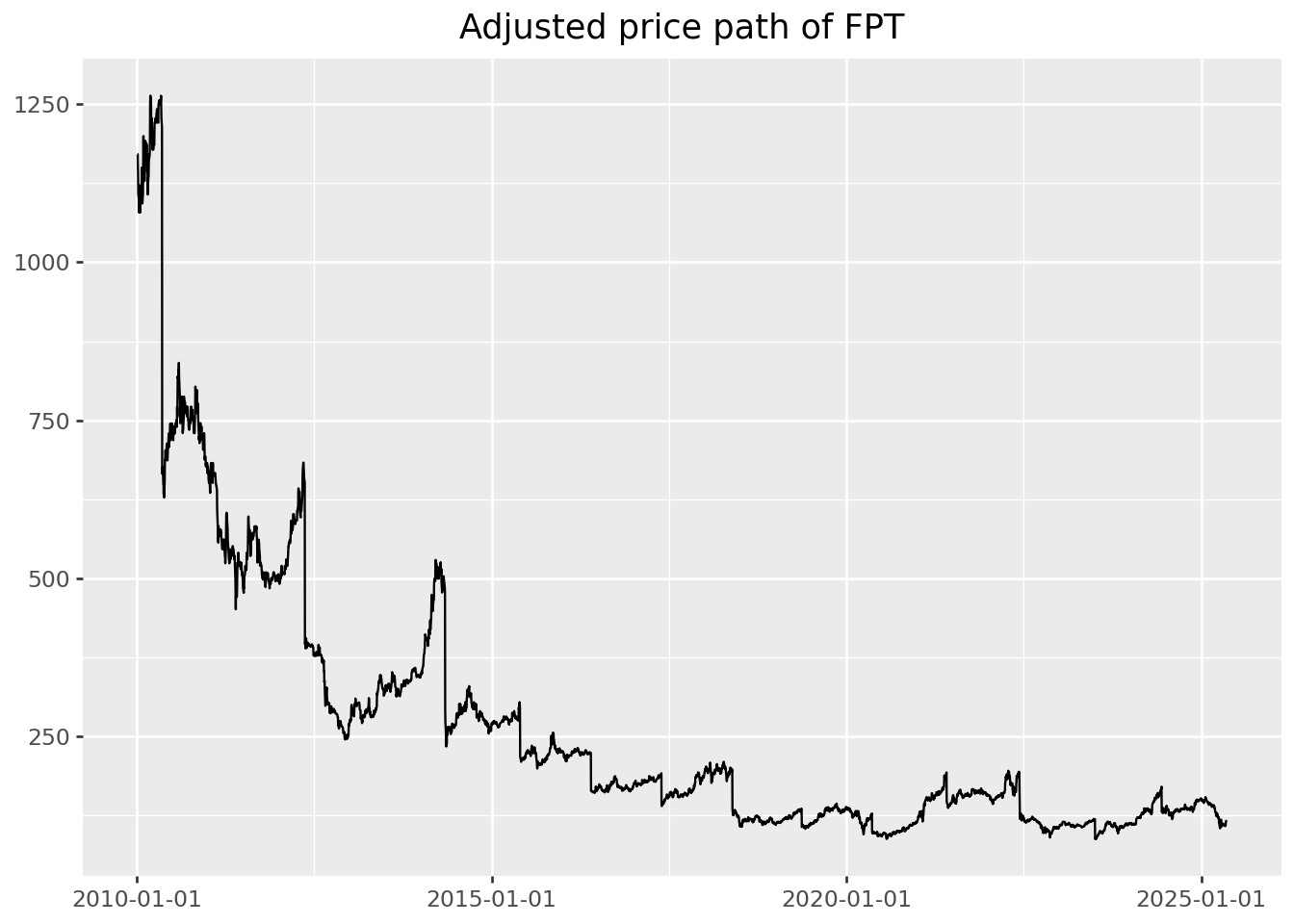
To ground the discussion, we isolate the trading history of a single large-cap stock, FPT, over a long sample period.
import datetime as dt

start = pd.Timestamp("2000-01-01")
end = pd.Timestamp(dt.date.today().year - 1, 12, 31)


fpt = prices.loc[
    (prices["symbol"] == "FPT")
    & (prices["date"] >= start)
    & (prices["date"] <= end),
    ["date", "symbol", "volume", "open", "low", "high", "close", "adjusted_close"],
].copy()
This subset contains the standard daily market variables required for most empirical studies. Before computing returns, it is good practice to visually inspect the price series.
from plotnine import ggplot, aes, geom_line, labs(
ggplot(fpt, aes(x="date", y="adjusted_close"))
+ geom_line()
+ labs(title="Adjusted price path of FPT", x="", y="")
)
6.3 From Prices to Returns
Most empirical asset pricing models are formulated in terms of returns rather than price levels. The simple daily return is defined as
\[ r_t = \frac{p_t}{p_t - 1} - 1, \]
where \(p_t\) denotes the adjusted closing price at the end of trading day \(t\).
Before computing returns, we must address invalid price observations. In Vietnamese equity data, adjusted prices occasionally take the value zero. These entries typically arise from IPO placeholders, trading suspensions, or historical backfilling conventions and cannot be used to compute meaningful returns.
prices.loc[prices["adjusted_close"] <= 0, ["symbol", "date", "adjusted_close"]].head()| symbol | date | adjusted_close | |
|---|---|---|---|
| 33886 | ADP | 2010-02-09 | 0.0 |
| 33887 | ADP | 2010-02-24 | 0.0 |
| 33888 | ADP | 2010-03-01 | 0.0 |
| 33889 | ADP | 2010-03-03 | 0.0 |
| 33890 | ADP | 2010-03-12 | 0.0 |
We therefore exclude non-positive adjusted prices and compute returns stock by stock. Correct chronological ordering is essential.
returns = (
    prices
    .loc[prices["adjusted_close"] > 0]
    .sort_values(["symbol", "date"])
    .assign(ret=lambda x: x.groupby("symbol")["adjusted_close"].pct_change())
    [["symbol", "date", "ret"]]
)
returns = returns.dropna(subset=["ret"])
The initial return for each stock is missing by construction, since no lagged price is available. These observations are mechanical and can safely be removed in most applications.
6.4 Limiting the Influence of Extreme Returns
Daily return series often contain extreme observations driven by data errors, thin trading, or abrupt price adjustments. A common approach is to winsorize returns using cross-sectional percentile cutoffs.
def winsorize_cs(df, column="ret", lower_q=0.01, upper_q=0.99):
    lo = df[column].quantile(lower_q)
    hi = df[column].quantile(upper_q)
    out = df.copy()
    out[column] = out[column].clip(lo, hi)
    return out

returns = winsorize_cs(returns)
Applying winsorization across the full cross-section limits the impact of extreme market-wide observations while preserving relative differences between firms. Winsorizing within each stock is rarely appropriate in panel settings and can severely distort illiquid securities.
6.5 Distributional Features of Returns
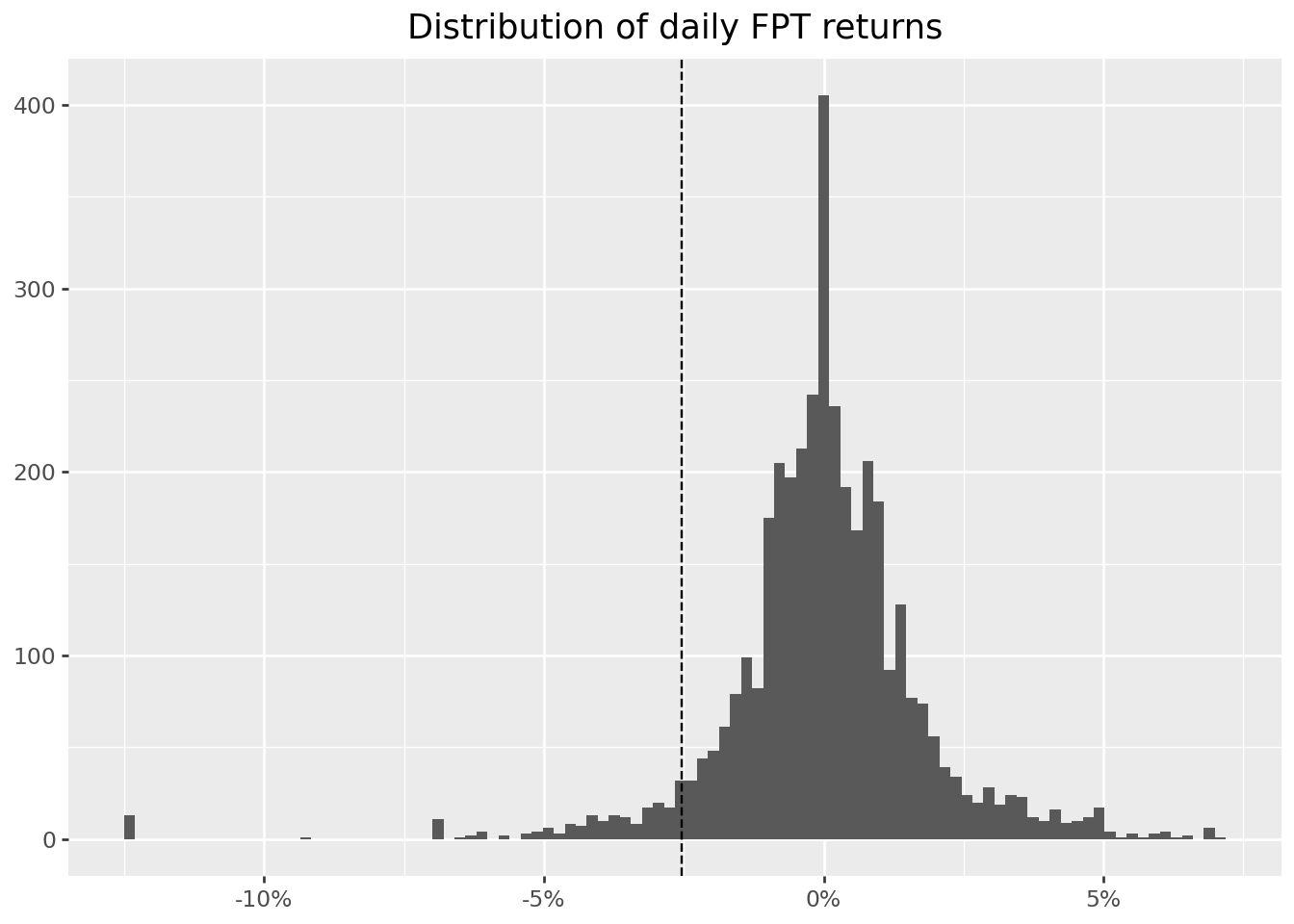
We next examine the empirical distribution of daily returns for FPT. The figure below also marks the historical 5 percent quantile, which provides a simple, non-parametric measure of downside risk.
from mizani.formatters import percent_format
from plotnine import geom_histogram, geom_vline, scale_x_continuous


fpt_ret = returns.loc[returns["symbol"] == "FPT"].copy()
q05 = fpt_ret["ret"].quantile(0.05)
(
ggplot(fpt_ret, aes(x="ret"))
+ geom_histogram(bins=100)
+ geom_vline(xintercept=q05, linetype="dashed")
+ scale_x_continuous(labels=percent_format())
+ labs(title="Distribution of daily FPT returns", x="", y="")
)
Summary statistics offer a compact description of return behavior and should always be inspected before formal modeling.
returns["ret"].describe().round(3)count 4305063.000
mean 0.000
std 0.035
min -0.125
25% -0.004
50% 0.000
75% 0.003
max 0.130
Name: ret, dtype: float64Computing these statistics by calendar year can reveal periods of elevated volatility or structural change.
(
    returns
    .assign(year=lambda x: x["date"].dt.year)
    .groupby("year")["ret"]
    .describe()
    .round(3)
)| count | mean | std | min | 25% | 50% | 75% | max | |
|---|---|---|---|---|---|---|---|---|
| year | ||||||||
| 2010 | 131548.0 | -0.001 | 0.036 | -0.125 | -0.021 | 0.0 | 0.018 | 0.13 |
| 2011 | 166826.0 | -0.003 | 0.033 | -0.125 | -0.020 | 0.0 | 0.011 | 0.13 |
| 2012 | 177938.0 | 0.000 | 0.033 | -0.125 | -0.012 | 0.0 | 0.015 | 0.13 |
| 2013 | 180417.0 | 0.001 | 0.033 | -0.125 | -0.004 | 0.0 | 0.008 | 0.13 |
| 2014 | 181907.0 | 0.001 | 0.034 | -0.125 | -0.008 | 0.0 | 0.011 | 0.13 |
| 2015 | 197881.0 | 0.000 | 0.033 | -0.125 | -0.006 | 0.0 | 0.005 | 0.13 |
| 2016 | 227896.0 | 0.000 | 0.035 | -0.125 | -0.005 | 0.0 | 0.003 | 0.13 |
| 2017 | 283642.0 | 0.001 | 0.034 | -0.125 | -0.002 | 0.0 | 0.001 | 0.13 |
| 2018 | 329887.0 | 0.000 | 0.035 | -0.125 | 0.000 | 0.0 | 0.000 | 0.13 |
| 2019 | 352754.0 | 0.000 | 0.033 | -0.125 | 0.000 | 0.0 | 0.000 | 0.13 |
| 2020 | 369367.0 | 0.001 | 0.035 | -0.125 | 0.000 | 0.0 | 0.000 | 0.13 |
| 2021 | 379415.0 | 0.002 | 0.038 | -0.125 | -0.005 | 0.0 | 0.007 | 0.13 |
| 2022 | 387050.0 | -0.001 | 0.038 | -0.125 | -0.008 | 0.0 | 0.004 | 0.13 |
| 2023 | 391605.0 | 0.001 | 0.034 | -0.125 | -0.002 | 0.0 | 0.002 | 0.13 |
| 2024 | 400379.0 | 0.000 | 0.031 | -0.125 | -0.002 | 0.0 | 0.000 | 0.13 |
| 2025 | 146551.0 | 0.000 | 0.037 | -0.125 | -0.004 | 0.0 | 0.002 | 0.13 |
6.6 Expanding to a Market Cross-Section
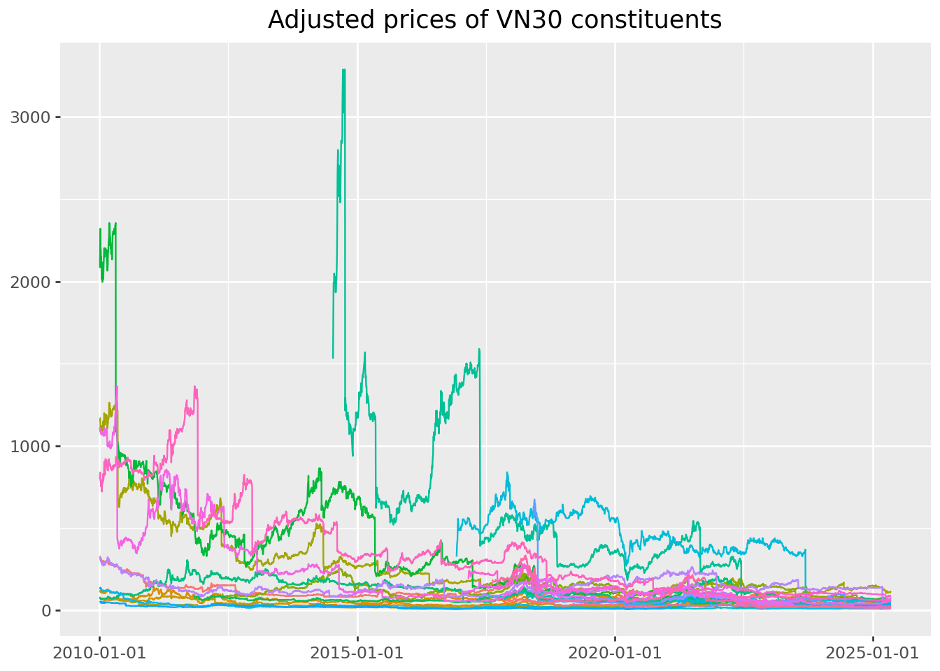
The same procedures apply naturally to a larger universe of stocks. We now restrict attention to the constituents of the VN30 index.
vn30 = [
    "ACB","BCM","BID","BVH","CTG","FPT","GAS","GVR","HDB","HPG",
    "MBB","MSN","MWG","PLX","POW","SAB","SHB","SSB","STB","TCB",
    "TPB","VCB","VHM","VIB","VIC","VJC","VNM","VPB","VRE","EIB",
]


prices_vn30 = prices.loc[prices["symbol"].isin(vn30)]
from plotnine import theme
(
ggplot(prices_vn30, aes(x="date", y="adjusted_close", color="symbol"))
+ geom_line()
+ labs(title="Adjusted prices of VN30 constituents", x="", y="")
+ theme(legend_position="none")
)
Returns for the VN30 universe are computed analogously.
returns_vn30 = (
    prices_vn30
    .sort_values(["symbol", "date"])
    .assign(ret=lambda x: x.groupby("symbol")["adjusted_close"].pct_change())
    [["symbol", "date", "ret"]]
    .dropna()
)


returns_vn30.groupby("symbol")["ret"].describe().round(3)| count | mean | std | min | 25% | 50% | 75% | max | |
|---|---|---|---|---|---|---|---|---|
| symbol | ||||||||
| ACB | 3822.0 | -0.000 | 0.023 | -0.407 | -0.006 | 0.0 | 0.007 | 0.097 |
| BCM | 1795.0 | 0.001 | 0.027 | -0.136 | -0.010 | 0.0 | 0.010 | 0.159 |
| BID | 2811.0 | 0.000 | 0.024 | -0.369 | -0.010 | 0.0 | 0.011 | 0.070 |
| BVH | 3825.0 | 0.000 | 0.024 | -0.097 | -0.012 | 0.0 | 0.012 | 0.070 |
| CTG | 3825.0 | 0.000 | 0.024 | -0.376 | -0.010 | 0.0 | 0.010 | 0.070 |
| EIB | 3825.0 | -0.000 | 0.022 | -0.302 | -0.008 | 0.0 | 0.008 | 0.070 |
| FPT | 3825.0 | -0.000 | 0.024 | -0.439 | -0.008 | 0.0 | 0.009 | 0.070 |
| GAS | 3236.0 | 0.000 | 0.022 | -0.289 | -0.009 | 0.0 | 0.010 | 0.070 |
| GVR | 1775.0 | 0.001 | 0.030 | -0.137 | -0.014 | 0.0 | 0.016 | 0.169 |
| HDB | 1828.0 | -0.001 | 0.028 | -0.391 | -0.009 | 0.0 | 0.010 | 0.070 |
| HPG | 3825.0 | -0.001 | 0.032 | -0.581 | -0.010 | 0.0 | 0.011 | 0.070 |
| MBB | 3371.0 | -0.000 | 0.023 | -0.473 | -0.008 | 0.0 | 0.008 | 0.069 |
| MSN | 3825.0 | 0.000 | 0.024 | -0.553 | -0.010 | 0.0 | 0.010 | 0.070 |
| MWG | 2701.0 | -0.000 | 0.035 | -0.751 | -0.009 | 0.0 | 0.011 | 0.070 |
| PLX | 2009.0 | -0.000 | 0.021 | -0.140 | -0.010 | 0.0 | 0.010 | 0.070 |
| POW | 1784.0 | 0.000 | 0.023 | -0.071 | -0.012 | 0.0 | 0.011 | 0.102 |
| SAB | 2100.0 | -0.000 | 0.024 | -0.745 | -0.008 | 0.0 | 0.007 | 0.070 |
| SHB | 3824.0 | -0.000 | 0.028 | -0.338 | -0.013 | 0.0 | 0.013 | 0.100 |
| SSB | 1029.0 | -0.000 | 0.023 | -0.292 | -0.005 | 0.0 | 0.004 | 0.070 |
| STB | 3825.0 | 0.000 | 0.024 | -0.321 | -0.010 | 0.0 | 0.010 | 0.070 |
| TCB | 1732.0 | -0.000 | 0.035 | -0.884 | -0.009 | 0.0 | 0.010 | 0.070 |
| TPB | 1761.0 | -0.001 | 0.029 | -0.477 | -0.009 | 0.0 | 0.009 | 0.070 |
| VCB | 3825.0 | -0.000 | 0.024 | -0.539 | -0.009 | 0.0 | 0.009 | 0.070 |
| VHM | 1744.0 | -0.000 | 0.024 | -0.419 | -0.009 | 0.0 | 0.008 | 0.070 |
| VIB | 2072.0 | -0.000 | 0.031 | -0.489 | -0.009 | 0.0 | 0.010 | 0.109 |
| VIC | 3825.0 | -0.000 | 0.027 | -0.673 | -0.008 | 0.0 | 0.008 | 0.070 |
| VJC | 2046.0 | -0.000 | 0.020 | -0.455 | -0.007 | 0.0 | 0.006 | 0.070 |
| VNM | 3825.0 | -0.000 | 0.023 | -0.547 | -0.007 | 0.0 | 0.007 | 0.070 |
| VPB | 1927.0 | -0.000 | 0.033 | -0.678 | -0.010 | 0.0 | 0.010 | 0.070 |
| VRE | 1871.0 | -0.000 | 0.024 | -0.295 | -0.012 | 0.0 | 0.011 | 0.070 |
6.7 Aggregating Returns Across Time
Financial variables are observed at different frequencies. While equity prices are recorded daily, many empirical questions require monthly or annual returns. Lower-frequency returns are constructed by compounding higher-frequency observations.
returns_monthly = (
returns_vn30
.assign(month=lambda x: x["date"].dt.to_period("M").dt.to_timestamp())
.groupby(["symbol", "month"], as_index=False)
.agg(ret=("ret", lambda x: np.prod(1 + x) - 1))
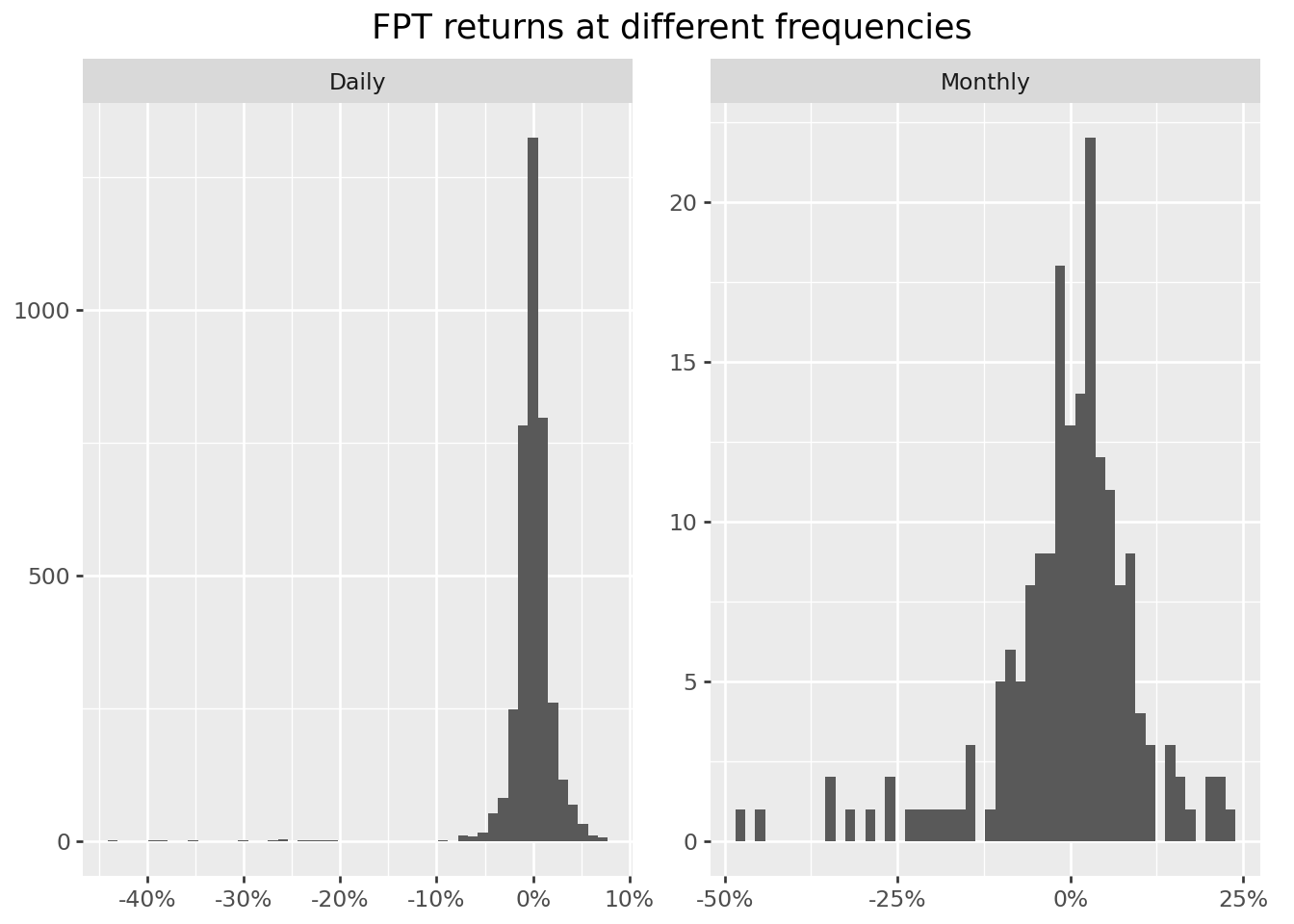
)Comparing daily and monthly return distributions illustrates how aggregation dampens volatility and alters tail behavior.
from plotnine import facet_wrap

fpt_d = returns_vn30.loc[returns_vn30["symbol"] == "FPT"].assign(freq="Daily")
fpt_m = returns_monthly.loc[returns_monthly["symbol"] == "FPT"].assign(freq="Monthly")


fpt_both = pd.concat([
    fpt_d[["ret", "freq"]],
    fpt_m[["ret", "freq"]],
])
(
ggplot(fpt_both, aes(x="ret"))
+ geom_histogram(bins=50)
+ scale_x_continuous(labels=percent_format())
+ labs(title="FPT returns at different frequencies", x="", y="")
+ facet_wrap("freq", scales="free")
)
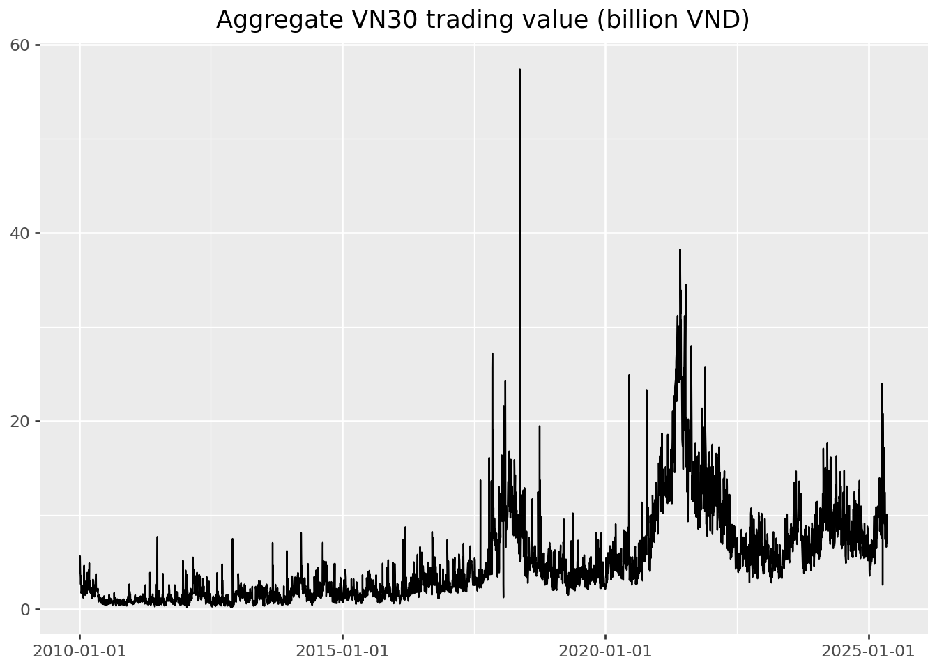
6.8 Aggregation Across Firms: Trading Activity
Aggregation is not limited to time. In some settings, it is informative to aggregate variables across firms. As an illustration, we compute total daily trading value for VN30 stocks by multiplying share volume by adjusted prices and summing across firms.
trading_value = (
    prices_vn30
    .assign(value=lambda x: x["volume"] * x["adjusted_close"] / 1e9)
    .groupby("date")["value"]
    .sum()
    .reset_index()
    .assign(value_lag=lambda x: x["value"].shift(1))
)
(
    ggplot(trading_value, aes(x="date", y="value"))
    + geom_line()
    + labs(title="Aggregate VN30 trading value (billion VND)", x="", y="")
)
Finally, we assess persistence in trading activity by comparing trading value on consecutive days.
from plotnine import geom_point, geom_abline(
ggplot(trading_value, aes(x="value_lag", y="value"))
+ geom_point()
+ geom_abline(intercept=0, slope=1, linetype="dashed")
+ labs(
title="Persistence in VN30 trading value",
x="Previous day",
y="Current day",
)
)/home/mikenguyen/project/tidyfinance/.venv/lib/python3.13/site-packages/plotnine/layer.py:374: PlotnineWarning: geom_point : Removed 1 rows containing missing values.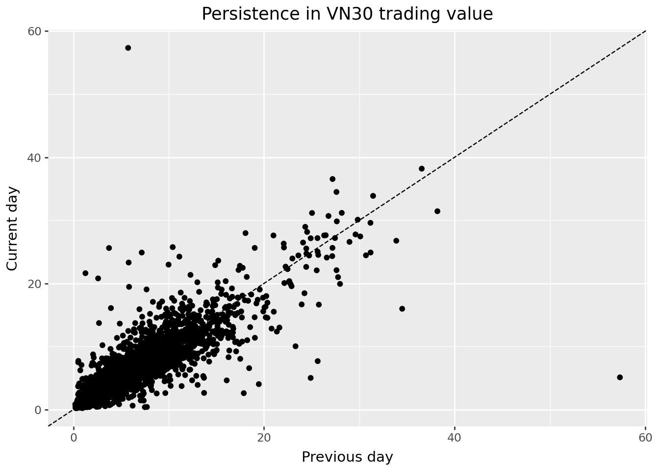
A strong alignment along the 45-degree line indicates that high-activity trading days tend to be followed by similarly active days, a common empirical regularity in equity markets.
6.9 Summary
This chapter established a reproducible workflow for transforming raw price data into return series, diagnosing common data issues, and aggregating information across time and firms. These steps provide the empirical foundation for subsequent analyses of risk, return predictability, and market dynamics in Vietnam’s equity market.