In this chapter, we implement and compare the two dominant approaches to testing asset pricing models: time-series regressions (do factors explain individual stock or portfolio returns?) and cross-sectional regressions (do factor exposures explain expected returns?), and develop the diagnostic tools to understand when and why they disagree.
Every factor model makes two distinct claims. The time-series claim is that a set of factors explains the common variation in individual stock returns (i.e., when the factors move, stocks move with them in proportion to their exposures). The cross-sectional claim is that differences in average returns across stocks are explained by differences in their factor exposures (i.e., stocks that load more heavily on a factor earn higher (or lower) average returns in proportion to the factor’s risk premium).
These claims are logically related but empirically distinct. A factor can explain time-series variation without explaining the cross-section (if the factor’s risk premium is zero, exposure to it creates no return differential). Conversely, a characteristic can predict the cross-section of returns without operating through a traded factor (if the characteristic captures mispricing rather than risk).
Fama and French (2020) formalize this distinction and show that the two approaches can give materially different answers about which factors matter. Goyal and Jegadeesh (2018) go further and demonstrate that time-series and cross-sectional tests can disagree about the same model (e.g., a factor can have a significant time-series alpha in one test and an insignificant cross-sectional premium in the other, or vice versa). Understanding why they disagree is essential for interpreting asset pricing evidence.
This chapter equips the reader with both toolkits, applied to Vietnamese data, and develops the intuition for when each is appropriate.
22.1 The Two Testing Frameworks
22.1.1 Time-Series Regressions
The time-series approach tests whether a factor model explains the returns of a set of test assets (typically portfolios). For each test asset \(i\), estimate:
where \(f_{k,t}\) are the \(K\) factor returns. The intercept \(\alpha_i\) measures the average return of asset \(i\) that is not explained by the factors. Under the null that the model correctly prices asset \(i\), \(\alpha_i = 0\).
The joint test of \(H_0: \alpha_1 = \alpha_2 = \ldots = \alpha_N = 0\) across all \(N\) test assets is performed using the Gibbons, Ross, and Shanken (1989) (GRS) test statistic:
\[
\text{GRS} = \frac{T - N - K}{N} \cdot \frac{1}{1 + \bar{f}' \hat{\Sigma}_f^{-1} \bar{f}} \cdot \hat{\alpha}' \hat{\Sigma}_\varepsilon^{-1} \hat{\alpha} \sim F(N, T - N - K)
\tag{22.2}\]
where \(\bar{f}\) is the vector of factor means, \(\hat{\Sigma}_f\) is the factor covariance matrix, and \(\hat{\Sigma}_\varepsilon\) is the residual covariance matrix. A large GRS statistic rejects the model.
22.1.2 Cross-Sectional Regressions (Fama-MacBeth)
The Fama and MacBeth (1973) cross-sectional approach tests whether factor exposures are priced (i.e., whether stocks with higher betas on a factor earn higher average returns). The procedure has two stages:
Stage 1 (Time-Series). For each asset, estimate factor betas from a time-series regression over a rolling or full-sample window:
The time-series averages \(\bar{\gamma}_k = \frac{1}{T} \sum_t \gamma_{k,t}\) estimate the risk premia, and the standard errors use the time-series standard deviation of \(\{\gamma_{k,t}\}\).
22.1.3 Key Differences
Table 22.1: Comparison of time-series and cross-sectional testing frameworks.
Dimension
Time-Series
Cross-Section
What it tests
Do factors explain return variation?
Do factor exposures explain average returns?
Key statistic
Alpha (intercept)
Risk premium (\(\gamma\))
Joint test
GRS F-test
Chi-squared on \(\gamma\)’s
Test assets
Portfolios (usually)
Individual stocks or portfolios
Factors
Must be traded returns
Can be non-traded (macro, characteristics)
Null hypothesis
\(\alpha_i = 0\) for all \(i\)
\(\gamma_k\) equals factor mean return
Errors-in-variables
Not an issue (factors observed)
Estimated betas create EIV bias
22.2 Data Construction
Import libraries and configure environment
import pandas as pdimport numpy as npimport matplotlib.pyplot as pltimport seaborn as snsimport statsmodels.api as smfrom scipy import statsfrom scipy.linalg import invimport warningswarnings.filterwarnings('ignore')plt.rcParams.update({'figure.figsize': (12, 6),'figure.dpi': 150,'font.size': 11,'axes.spines.top': False,'axes.spines.right': False})
Load factor returns, test portfolios, and individual stock data
Prepare excess return matrices for test portfolios
# Convert test portfolios to excess returns# Each portfolio set is a DataFrame: rows = months, columns = portfoliosdef prepare_test_assets(port_df, rf_df):"""Convert portfolio returns to excess returns matrix.""" port = port_df.set_index('month_end') rf_aligned = rf_df.set_index('month_end')['rf'].reindex(port.index) excess = port.subtract(rf_aligned, axis=0)return excess.dropna()excess_25_bm = prepare_test_assets(test_portfolios_25, rf)excess_25_mom = prepare_test_assets(test_portfolios_mom, rf)excess_10_ind = prepare_test_assets(test_portfolios_ind, rf)print(f"Size-BM test assets: {excess_25_bm.shape[1]} portfolios, "f"{excess_25_bm.shape[0]} months")print(f"Size-Mom test assets: {excess_25_mom.shape[1]} portfolios, "f"{excess_25_mom.shape[0]} months")print(f"Industry test assets: {excess_10_ind.shape[1]} portfolios, "f"{excess_10_ind.shape[0]} months")
22.3 Time-Series Tests
22.3.1 Full-Sample Time-Series Regressions
We begin by running full-sample time-series regressions of each test portfolio on the Fama-French five-factor model plus momentum:
Run time-series regressions for all test portfolios
def time_series_regressions(excess_returns, factor_df, factor_cols, cov_type='HAC', maxlags=6):""" Run time-series regressions of test assets on factors. Returns DataFrame of alphas, betas, t-stats, and R-squared. """# Align dates common = excess_returns.index.intersection(factor_df.index) Y = excess_returns.loc[common] X = factor_df.loc[common, factor_cols] X_const = sm.add_constant(X) results = {}for col in Y.columns: y = Y[col].dropna() x = X_const.loc[y.index] model = sm.OLS(y, x).fit( cov_type=cov_type, cov_kwds={'maxlags': maxlags} if cov_type =='HAC'else {} ) result = {'alpha': model.params['const'],'alpha_t': model.tvalues['const'],'alpha_p': model.pvalues['const'],'r_squared': model.rsquared,'r_squared_adj': model.rsquared_adj }for f in factor_cols: result[f'beta_{f}'] = model.params[f] result[f't_{f}'] = model.tvalues[f] results[col] = resultreturn pd.DataFrame(results).T# Define models to testmodels = {'CAPM': ['mkt_excess'],'FF3': ['mkt_excess', 'smb', 'hml'],'FF5': ['mkt_excess', 'smb', 'hml', 'rmw', 'cma'],'FF5+WML': ['mkt_excess', 'smb', 'hml', 'rmw', 'cma', 'wml'],}# Run for 25 Size-BM portfoliosprint("Time-Series Alphas: 25 Size-BM Portfolios")print("="*60)ts_results = {}for model_name, factor_cols in models.items(): result = time_series_regressions( excess_25_bm, factors, factor_cols ) ts_results[model_name] = result mean_alpha = result['alpha'].mean() *12 mean_abs_alpha = result['alpha'].abs().mean() *12 pct_sig = (result['alpha_p'] <0.05).mean() mean_r2 = result['r_squared'].mean()print(f"\n{model_name}:")print(f" Mean alpha (ann.): {mean_alpha:.4f}")print(f" Mean |alpha| (ann.): {mean_abs_alpha:.4f}")print(f" % sig. at 5%: {pct_sig:.1%}")print(f" Mean R²: {mean_r2:.3f}")
22.3.2 The GRS Test
Implement and compute the GRS test statistic
def grs_test(excess_returns, factor_df, factor_cols):""" Gibbons, Ross, Shanken (1989) test of H0: all alphas = 0. Returns GRS statistic, p-value, and related diagnostics. """ common = excess_returns.index.intersection(factor_df.index) Y = excess_returns.loc[common].values # T x N F = factor_df.loc[common, factor_cols].values # T x K T, N = Y.shape K = F.shape[1]# Add constant and run OLS for each asset F_const = np.column_stack([np.ones(T), F])# OLS: beta = (X'X)^-1 X'Y XtX_inv = inv(F_const.T @ F_const) B = XtX_inv @ F_const.T @ Y # (K+1) x N alpha = B[0, :] # N-vector of intercepts residuals = Y - F_const @ B # T x N# Residual covariance matrix Sigma_eps = residuals.T @ residuals / (T - K -1)# Factor mean and covariance f_bar = F.mean(axis=0) Sigma_f = np.cov(F, rowvar=False, ddof=1)# GRS statistic Sigma_eps_inv = inv(Sigma_eps) Sigma_f_inv = inv(Sigma_f) if K >1else np.array([[1/ Sigma_f]]) sharpe_sq_alpha = alpha @ Sigma_eps_inv @ alpha sharpe_sq_f = f_bar @ Sigma_f_inv @ f_bar if K >1else (f_bar[0] **2/ Sigma_f) grs_stat = ((T - N - K) / N) * (1/ (1+ sharpe_sq_f)) * sharpe_sq_alpha# p-value from F distribution p_value =1- stats.f.cdf(grs_stat, N, T - N - K)# Additional diagnostics# Sharpe ratio of tangency portfolio of factors sr_factors = np.sqrt(sharpe_sq_f)# Sharpe ratio of tangency portfolio including alphas sr_alpha = np.sqrt(sharpe_sq_alpha + sharpe_sq_f)return {'GRS': grs_stat,'p_value': p_value,'df1': N,'df2': T - N - K,'mean_abs_alpha': np.abs(alpha).mean(),'sr_factors': sr_factors,'sr_alpha_plus_factors': sr_alpha,'sr_improvement': sr_alpha - sr_factors,'T': T, 'N': N, 'K': K }# Run GRS for each model on each set of test assetsprint("GRS Test Results")print("="*80)print(f"{'Model':<12}{'Test Assets':<18}{'GRS':>8}{'p-value':>10} "f"{'|α| ann':>10}{'SR(f)':>8}{'SR(α+f)':>8}")print("-"*80)test_asset_sets = {'25 Size-BM': excess_25_bm,'25 Size-Mom': excess_25_mom,'10 Industry': excess_10_ind}grs_all = {}for model_name, factor_cols in models.items():for ta_name, ta_data in test_asset_sets.items(): key =f"{model_name}_{ta_name}" result = grs_test(ta_data, factors, factor_cols) grs_all[key] = resultprint(f"{model_name:<12}{ta_name:<18} "f"{result['GRS']:>8.2f}{result['p_value']:>10.4f} "f"{result['mean_abs_alpha']*12:>10.4f} "f"{result['sr_factors']:>8.3f} "f"{result['sr_alpha_plus_factors']:>8.3f}")
Visualize GRS statistics across models and test assets
fig, ax = plt.subplots(figsize=(12, 5))model_names =list(models.keys())ta_names =list(test_asset_sets.keys())x = np.arange(len(model_names))width =0.25colors_ta = ['#2C5F8A', '#C0392B', '#27AE60']for i, ta_name inenumerate(ta_names): grs_vals = [grs_all[f"{m}_{ta_name}"]['GRS'] for m in model_names] bars = ax.bar(x + i * width, grs_vals, width, alpha=0.85, color=colors_ta[i], label=ta_name, edgecolor='white')ax.set_xticks(x + width)ax.set_xticklabels(model_names)ax.set_ylabel('GRS Statistic')ax.set_title('GRS Test: Model Comparison Across Test Asset Sets')ax.legend()# Add critical value line (5% significance)# Approximate: depends on N, T, Kax.axhline(y=1.8, color='gray', linestyle='--', linewidth=1, label='~5% critical value')plt.tight_layout()plt.show()
Figure 22.2
22.4 Cross-Sectional Tests
22.4.1 Fama-MacBeth with Portfolio Test Assets
We implement the Fama-MacBeth two-pass procedure using the 25 size-BM portfolios as test assets:
Full Fama-MacBeth two-pass procedure on portfolio test assets
def fama_macbeth_two_pass(excess_returns, factor_df, factor_cols, beta_window='full', rolling_window=60, shanken_correction=True):""" Fama-MacBeth (1973) two-pass cross-sectional regression. Parameters ---------- beta_window : str 'full' for full-sample betas, 'rolling' for rolling betas. shanken_correction : bool Apply Shanken (1992) errors-in-variables correction. Returns ------- Dictionary with estimated risk premia, t-statistics, and diagnostics. """ common = excess_returns.index.intersection(factor_df.index) Y = excess_returns.loc[common] F = factor_df.loc[common, factor_cols] T =len(common) N = Y.shape[1] K =len(factor_cols) months =sorted(common)# ===== STAGE 1: Estimate betas =====if beta_window =='full':# Full-sample betas (simpler, used in GRS context) F_const = sm.add_constant(F) betas = {}for col in Y.columns: model = sm.OLS(Y[col], F_const).fit() betas[col] = {f: model.params[f] for f in factor_cols} beta_df = pd.DataFrame(betas).T # N x K# Same betas used every month beta_by_month = {m: beta_df for m in months}elif beta_window =='rolling':# Rolling betas (more realistic, avoids look-ahead) beta_by_month = {}for t_idx inrange(rolling_window, T): month = months[t_idx] window_start = months[t_idx - rolling_window] Y_win = Y.loc[window_start:months[t_idx -1]] F_win = sm.add_constant(F.loc[window_start:months[t_idx -1]]) betas_t = {}for col in Y.columns: y = Y_win[col].dropna() x = F_win.loc[y.index]iflen(y) <24: betas_t[col] = {f: np.nan for f in factor_cols}continue model = sm.OLS(y, x).fit() betas_t[col] = {f: model.params[f] for f in factor_cols} beta_by_month[month] = pd.DataFrame(betas_t).T# ===== STAGE 2: Cross-sectional regressions ===== gamma_list = []for month in months:if month notin beta_by_month:continue betas_t = beta_by_month[month] returns_t = Y.loc[month]# Align valid = betas_t.dropna().index.intersection(returns_t.dropna().index)iflen(valid) < K +5:continue y = returns_t[valid].values X = sm.add_constant(betas_t.loc[valid, factor_cols].values)try: model = sm.OLS(y, X).fit() gammas = {'month': month, 'gamma_0': model.params[0]}for j, f inenumerate(factor_cols): gammas[f'gamma_{f}'] = model.params[j +1] gammas['r_squared'] = model.rsquared gammas['n_assets'] =len(valid) gamma_list.append(gammas)exceptException:pass gamma_df = pd.DataFrame(gamma_list)iflen(gamma_df) ==0:returnNone# ===== INFERENCE =====# Time-series averages of gammas gamma_cols = ['gamma_0'] + [f'gamma_{f}'for f in factor_cols] results = {}for col in gamma_cols: g = gamma_df[col] mean = g.mean() se_fm = g.std() / np.sqrt(len(g)) t_fm = mean / se_fm if se_fm >0else np.nan results[col] = {'estimate': mean,'se_fm': se_fm,'t_fm': t_fm, }# Shanken (1992) correction for errors-in-variablesif shanken_correction and beta_window =='full': Sigma_f = F[factor_cols].cov().values# Shanken correction factor: (1 + lambda' Sigma_f^-1 lambda) gamma_factor = np.array([results[f'gamma_{f}']['estimate']for f in factor_cols])try: Sigma_f_inv = inv(Sigma_f) c_shanken =1+ gamma_factor @ Sigma_f_inv @ gamma_factorexceptException: c_shanken =1.0for col in gamma_cols: results[col]['se_shanken'] = results[col]['se_fm'] * np.sqrt(c_shanken) results[col]['t_shanken'] = (results[col]['estimate']/ results[col]['se_shanken']if results[col]['se_shanken'] >0else np.nan)# Compare estimated premia to factor mean returns factor_means = F[factor_cols].mean()for f in factor_cols: results[f'gamma_{f}']['factor_mean'] = factor_means[f]# Cross-sectional R-squared results['avg_cs_r2'] = gamma_df['r_squared'].mean()return {'results': pd.DataFrame(results).T,'gamma_ts': gamma_df,'beta_df': beta_by_month.get(months[-1], None) }# Run Fama-MacBeth for each modelprint("Fama-MacBeth Cross-Sectional Results: 25 Size-BM Portfolios")print("="*80)fm_results = {}for model_name, factor_cols in models.items():for beta_type in ['full', 'rolling']: key =f"{model_name}_{beta_type}" fm = fama_macbeth_two_pass( excess_25_bm, factors, factor_cols, beta_window=beta_type, rolling_window=60, shanken_correction=(beta_type =='full') )if fm isNone:continue fm_results[key] = fmprint(f"\n{model_name} (betas: {beta_type}):") res = fm['results']for idx, row in res.iterrows():if'gamma'in idx: t_col ='t_shanken'if't_shanken'in row and pd.notna(row.get('t_shanken')) else't_fm' f_mean = row.get('factor_mean', '') f_str =f" f_mean={f_mean:.4f}"ifisinstance(f_mean, float) else""print(f" {idx:<16}: γ = {row['estimate']:.5f}, "f"t = {row[t_col]:.2f}{f_str}")if'avg_cs_r2'in res.index:print(f" Avg CS R²: {res.loc['avg_cs_r2', 'estimate']:.3f}")
22.4.2 The Shanken Correction
The Shanken (1992) correction addresses the errors-in-variables (EIV) problem inherent in the two-pass procedure. Because betas are estimated with error in Stage 1, the Stage 2 standard errors are understated. The correction inflates the standard errors by a factor that depends on the estimated risk premia and the factor covariance matrix:
Compare FM t-statistics with and without Shanken correction
print("Impact of Shanken Correction on t-statistics:")print(f"{'Model':<12}{'Factor':<12}{'t (FM)':>10}{'t (Shanken)':>12}{'Ratio':>8}")print("-"*54)for model_name in models: key =f"{model_name}_full"if key notin fm_results:continue res = fm_results[key]['results']for idx, row in res.iterrows():if'gamma_'instr(idx) and idx !='gamma_0': t_fm = row.get('t_fm', np.nan) t_sh = row.get('t_shanken', np.nan) ratio = t_fm / t_sh if pd.notna(t_sh) and t_sh !=0else np.nan factor_name = idx.replace('gamma_', '')print(f"{model_name:<12}{factor_name:<12}{t_fm:>10.2f} "f"{t_sh:>12.2f}{ratio:>8.2f}")
22.4.3 Fama-MacBeth with Individual Stocks
Using individual stocks instead of portfolios as test assets avoids the Lewellen, Nagel, and Shanken (2010) critique that sorted portfolios create artificially strong factor structure:
Fama-MacBeth regressions using individual stocks
def fama_macbeth_individual(stock_df, factor_df, factor_cols, beta_window=60, min_obs=36, min_stocks=100):""" Fama-MacBeth with individual stocks and rolling betas. """ stock_df = stock_df.copy() stock_df['month_end'] = pd.to_datetime(stock_df['month_end']) factor_df = factor_df.copy() months =sorted(stock_df['month_end'].unique())# Pre-compute rolling betas for all stocks gamma_list = []for t_idx, month inenumerate(months):if t_idx < beta_window:continue window_months = months[t_idx - beta_window:t_idx]# Get betas for each stock from rolling window betas_t = {} window_data = stock_df[stock_df['month_end'].isin(window_months)]for ticker, group in window_data.groupby('ticker'):iflen(group) < min_obs:continue y = group.set_index('month_end')['monthly_return'] x = factor_df.loc[y.index, factor_cols] x = sm.add_constant(x) valid = y.index.intersection(x.index)iflen(valid) < min_obs:continuetry: model = sm.OLS(y[valid], x.loc[valid]).fit() betas_t[ticker] = {f: model.params[f] for f in factor_cols}exceptException:passiflen(betas_t) < min_stocks:continue beta_df = pd.DataFrame(betas_t).T# Current month returns current = stock_df[stock_df['month_end'] == month] current = current.set_index('ticker')# Align valid_tickers = beta_df.index.intersection(current.index)iflen(valid_tickers) < min_stocks:continue y = current.loc[valid_tickers, 'monthly_return'].values X = sm.add_constant(beta_df.loc[valid_tickers].values)try: model = sm.OLS(y, X).fit() gammas = {'month': month, 'gamma_0': model.params[0]}for j, f inenumerate(factor_cols): gammas[f'gamma_{f}'] = model.params[j +1] gammas['n_stocks'] =len(valid_tickers) gammas['r_squared'] = model.rsquared gamma_list.append(gammas)exceptException:pass gamma_df = pd.DataFrame(gamma_list)# Inference gamma_cols = ['gamma_0'] + [f'gamma_{f}'for f in factor_cols] summary = {}for col in gamma_cols: g = gamma_df[col] mean = g.mean() se = g.std() / np.sqrt(len(g)) t = mean / se if se >0else np.nan summary[col] = {'estimate': mean, 'se': se, 't': t} summary['avg_n_stocks'] = gamma_df['n_stocks'].mean() summary['avg_cs_r2'] = gamma_df['r_squared'].mean()return pd.DataFrame(summary).T, gamma_df# Run for FF5print("\nFama-MacBeth with Individual Stocks (FF5):")fm_ind_results, fm_ind_gamma = fama_macbeth_individual( stock_returns, factors, ['mkt_excess', 'smb', 'hml', 'rmw', 'cma'], beta_window=60, min_obs=36)print(fm_ind_results.round(4).to_string())
22.5 When Do the Tests Disagree?
22.5.1 Theoretical Sources of Disagreement
Goyal and Jegadeesh (2018) identify three sources of discrepancy between time-series and cross-sectional tests:
1. Factor structure of test assets. If test assets have a strong factor structure (as sorted portfolios do by construction), the cross-sectional \(R^2\) will be high regardless of whether the factors truly price the assets. Lewellen, Nagel, and Shanken (2010) show that even random factors can achieve high cross-sectional \(R^2\) when test assets are size-BM sorted portfolios, because such portfolios have a strong linear structure in the size-value space.
2. Time-variation in betas. The time-series regression assumes constant betas. If betas vary over time and co-move with the factor risk premium, the unconditional time-series alpha can be nonzero even if the conditional model holds (Jagannathan and Wang 1996).
3. Misspecified risk premia. The Fama-MacBeth cross-sectional regression estimates the risk premium from the data. The time-series regression implicitly sets the risk premium equal to the factor’s sample mean return. When these differ (e.g., because the factor is not a perfect proxy for the underlying risk), the two approaches disagree.
22.5.2 Empirical Comparison for Vietnam
Compare time-series alphas with cross-sectional pricing errors
# For FF5 on 25 Size-BM portfolios:# Time-series: alpha from OLS regression# Cross-section: pricing error from Fama-MacBethts_alphas = ts_results['FF5']['alpha'].values *12# Annualizedts_names = ts_results['FF5'].index.tolist()# Cross-sectional pricing errors:# Predicted return = beta' * estimated_gamma# Pricing error = actual mean return - predictedfm_full = fm_results.get('FF5_full')if fm_full: betas = fm_full['beta_df'] # N x K factor_cols = ['mkt_excess', 'smb', 'hml', 'rmw', 'cma'] gammas = np.array([fm_full['results'].loc[f'gamma_{f}', 'estimate']for f in factor_cols]) gamma_0 = fm_full['results'].loc['gamma_0', 'estimate'] actual_means = excess_25_bm.mean() *12# Annualized predicted = (gamma_0 + betas[factor_cols].values @ gammas) *12 cs_errors = actual_means.values - predicted
Scatter plot comparing TS alphas and CS pricing errors
Lewellen, Nagel, and Shanken (2010) demonstrate that the high cross-sectional \(R^2\) from Fama-MacBeth regressions on sorted portfolios can be misleading. Sorted portfolios have a strong factor structure by construction, so even irrelevant factors can produce high \(R^2\). They recommend:
Including industry portfolios alongside sorted portfolios to break the mechanical factor structure.
Constraining the estimated risk premia to equal the factor mean returns (this is what the time-series test implicitly does).
Reporting the cross-sectional \(R^2\) from the constrained model alongside the unconstrained estimate.
Implement the Lewellen-Nagel-Shanken diagnostic
def lns_diagnostic(excess_returns, factor_df, factor_cols):""" Lewellen-Nagel-Shanken (2010) diagnostic: Compare unconstrained CS R² to constrained (factor mean = premium). """ common = excess_returns.index.intersection(factor_df.index) Y = excess_returns.loc[common] F = factor_df.loc[common, factor_cols]# Full-sample betas betas = {} F_const = sm.add_constant(F)for col in Y.columns: model = sm.OLS(Y[col], F_const).fit() betas[col] = {f: model.params[f] for f in factor_cols} beta_mat = pd.DataFrame(betas).T # N x K actual = Y.mean() *12# Annualized# Unconstrained: FM regression X = sm.add_constant(beta_mat.values) fm_model = sm.OLS(actual.values, X).fit() predicted_unc = fm_model.fittedvalues r2_unconstrained = fm_model.rsquared# Constrained: premium = factor mean return factor_means = F.mean().values *12# Annualized predicted_con = beta_mat.values @ factor_means# Add best-fitting intercept intercept_con = np.mean(actual.values - predicted_con) predicted_con += intercept_con ss_res_con = np.sum((actual.values - predicted_con) **2) ss_tot = np.sum((actual.values - actual.values.mean()) **2) r2_constrained =1- ss_res_con / ss_totreturn {'r2_unconstrained': r2_unconstrained,'r2_constrained': r2_constrained,'r2_drop': r2_unconstrained - r2_constrained,'gamma_unconstrained': fm_model.params[1:],'gamma_constrained': factor_means }print("Lewellen-Nagel-Shanken Diagnostic:")print(f"{'Model':<12}{'Test Assets':<18}{'R² (unc)':>10}{'R² (con)':>10} "f"{'Drop':>8}")print("-"*58)for model_name, factor_cols in models.items():for ta_name, ta_data in test_asset_sets.items(): diag = lns_diagnostic(ta_data, factors, factor_cols)print(f"{model_name:<12}{ta_name:<18} "f"{diag['r2_unconstrained']:>10.3f} "f"{diag['r2_constrained']:>10.3f} "f"{diag['r2_drop']:>8.3f}")
Visualize constrained vs unconstrained cross-sectional fit
Both time-series and cross-sectional tests are special cases of the Hansen (1982) Generalized Method of Moments (GMM) framework. The fundamental pricing equation is:
\[
E[M_t R_{i,t}^e] = 0 \quad \text{for all } i
\tag{22.6}\]
where \(M_t\) is the stochastic discount factor (SDF) and \(R_{i,t}^e\) is the excess return of asset \(i\). A linear factor model parameterizes the SDF as:
\[
M_t = 1 - b' (f_t - \mu_f)
\tag{22.7}\]
where \(b\) is the vector of SDF loadings and \(f_t\) are the factors. The GMM approach estimates \(b\) by minimizing the quadratic form of the pricing errors:
\[
\hat{b} = \arg\min_b \ g(b)' W \ g(b)
\tag{22.8}\]
where \(g(b) = \frac{1}{T} \sum_t M_t(b) R_t^e\) is the sample analog of the moment conditions.
Implement GMM estimation of the linear SDF model
def gmm_sdf(excess_returns, factor_df, factor_cols, weighting='identity', n_iter=2):""" GMM estimation of the linear SDF model. Parameters ---------- weighting : str 'identity': first-stage identity weighting matrix 'optimal': Hansen optimal weighting (iterated) n_iter : int Number of GMM iterations (2 = efficient two-step) """ common = excess_returns.index.intersection(factor_df.index) Re = excess_returns.loc[common].values # T x N F = factor_df.loc[common, factor_cols].values # T x K T, N = Re.shape K = F.shape[1]# Demean factors F_dm = F - F.mean(axis=0)# Moment conditions: E[M * Re] = 0# M = 1 - b' (f - mu_f) = 1 - b' F_dmdef pricing_errors(b): M =1- F_dm @ b # T-vector g = (M[:, np.newaxis] * Re).mean(axis=0) # N-vectorreturn g# GMM objective W = np.eye(N) # Initial weighting matrixfrom scipy.optimize import minimizefor iteration inrange(n_iter):def objective(b): g = pricing_errors(b)return T * g @ W @ g result = minimize(objective, np.zeros(K), method='L-BFGS-B') b_hat = result.xif iteration < n_iter -1:# Update weighting matrix (Hansen optimal) g_t = np.array([(1- F_dm[t] @ b_hat) * Re[t]for t inrange(T)]) # T x N S = np.cov(g_t, rowvar=False, ddof=0)# Newey-West adjustment for serial correlation max_lag =int(np.floor(4* (T /100) ** (2/9)))for lag inrange(1, max_lag +1): w =1- lag / (max_lag +1) Gamma = np.cov(g_t[lag:].T, g_t[:-lag].T, ddof=0)[:N, N:] S += w * (Gamma + Gamma.T)try: W = inv(S)exceptException: W = np.eye(N)# Pricing errors at optimum g_hat = pricing_errors(b_hat)# Implied risk premia: lambda = Sigma_f @ b Sigma_f = np.cov(F, rowvar=False, ddof=1) lambda_hat = Sigma_f @ b_hat# J-test (overidentification) J = T * g_hat @ W @ g_hat df_J = N - K p_J =1- stats.chi2.cdf(J, df_J) if df_J >0else np.nan# HJ distance (model misspecification) hj_dist = np.sqrt(g_hat @ inv(np.cov(Re, rowvar=False)) @ g_hat)return {'b_hat': b_hat,'lambda_hat': lambda_hat,'pricing_errors': g_hat,'J_stat': J,'J_pvalue': p_J,'J_df': df_J,'hj_distance': hj_dist,'mean_abs_error': np.abs(g_hat).mean() *12 }print("GMM SDF Estimation:")print(f"{'Model':<12}{'Test Assets':<18}{'J-stat':>8}{'J p-val':>10} "f"{'HJ dist':>8}{'|e| ann':>10}")print("-"*66)for model_name, factor_cols in models.items():for ta_name, ta_data in test_asset_sets.items(): gmm = gmm_sdf(ta_data, factors, factor_cols, n_iter=2)print(f"{model_name:<12}{ta_name:<18} "f"{gmm['J_stat']:>8.2f}{gmm['J_pvalue']:>10.4f} "f"{gmm['hj_distance']:>8.4f}{gmm['mean_abs_error']:>10.4f}")# Print implied risk premiafor j, f inenumerate(factor_cols):print(f" λ_{f}: {gmm['lambda_hat'][j]*12:.4f} "f"(factor mean: {factors[f].mean()*12:.4f})")
22.7 Model Comparison
22.7.1 The Barillas-Shanken Framework
Barillas and Shanken (2018) propose a Bayesian framework for comparing non-nested factor models. The key insight is that model comparison should be based on the factors’ ability to explain each other’s returns, not on their ability to price a fixed set of test assets. Two models differ only in their excluded factors, so the relevant comparison is whether the factors unique to each model have alpha with respect to the other model.
Implement Barillas-Shanken model comparison
def barillas_shanken_compare(factor_df, model_a_cols, model_b_cols):""" Barillas-Shanken (2018) pairwise model comparison. Compare Model A vs Model B by testing whether the factors unique to each model have alpha with respect to the other. """# Factors unique to each model unique_a = [f for f in model_a_cols if f notin model_b_cols] unique_b = [f for f in model_b_cols if f notin model_a_cols] results = {}# Test: do factors unique to A have alpha w.r.t. B?# If yes, A adds value beyond Bif unique_a:for f in unique_a: y = factor_df[f] X = sm.add_constant(factor_df[model_b_cols]) common = y.dropna().index.intersection(X.dropna().index) model = sm.OLS(y[common], X.loc[common]).fit( cov_type='HAC', cov_kwds={'maxlags': 6} ) results[f'alpha_{f}_vs_B'] = {'alpha': model.params['const'] *12,'t': model.tvalues['const'],'r2': model.rsquared }if unique_b:for f in unique_b: y = factor_df[f] X = sm.add_constant(factor_df[model_a_cols]) common = y.dropna().index.intersection(X.dropna().index) model = sm.OLS(y[common], X.loc[common]).fit( cov_type='HAC', cov_kwds={'maxlags': 6} ) results[f'alpha_{f}_vs_A'] = {'alpha': model.params['const'] *12,'t': model.tvalues['const'],'r2': model.rsquared }return pd.DataFrame(results).T# Compare FF3 vs FF5print("Barillas-Shanken: FF3 vs FF5")bs_3v5 = barillas_shanken_compare( factors, ['mkt_excess', 'smb', 'hml'], ['mkt_excess', 'smb', 'hml', 'rmw', 'cma'])print(bs_3v5.round(4).to_string())# Compare FF5 vs FF5+WMLprint("\nBarillas-Shanken: FF5 vs FF5+WML")bs_5vw = barillas_shanken_compare( factors, ['mkt_excess', 'smb', 'hml', 'rmw', 'cma'], ['mkt_excess', 'smb', 'hml', 'rmw', 'cma', 'wml'])print(bs_5vw.round(4).to_string())# Compare FF3+WML vs FF5+WMLprint("\nBarillas-Shanken: FF3+WML vs FF5+WML")bs_3wv5w = barillas_shanken_compare( factors, ['mkt_excess', 'smb', 'hml', 'wml'], ['mkt_excess', 'smb', 'hml', 'rmw', 'cma', 'wml'])print(bs_3wv5w.round(4).to_string())
The Barillas-Shanken framework compares two models at a time. But the factor zoo (Section 21.1) offers dozens of candidate factors, and the practical question is not “is model A better than model B?” but “which subset of all available factors constitutes the best model?” Feng et al. (2026) answer this with a stepwise selection procedure that builds a factor model sequentially, adding and removing factors on the basis of asset-pricing tests, and that tests the resulting model against both the test assets and the factors it left out. Applied to US data, their procedure rejects the workhorse models (CAPM, the Fama-French three- and five-factor models) and selects an eight-factor model that survives the pricing tests and performs robustly out of sample. This section develops the method from first principles and provides a complete, runnable implementation.
The intellectual lineage is worth naming. Feng, Giglio, and Xiu (2020) (“Taming the Factor Zoo”) use double-selection LASSO to test whether a new factor earns a risk premium after controlling for a high-dimensional set of existing ones. Feng et al. (2026) instead select the model itself, and their stopping rule leans on the observation—formalized by Barillas and Shanken (2018)—that comparing factor models reduces to comparing the maximum squared Sharpe ratios their factors attain.
22.8.1 The Squared-Sharpe-Ratio Spanning Duality
The engine of the method is a duality between mean-variance efficiency and the spanning regressions of the previous section. For a set of factors \(F\) with mean vector \(\boldsymbol{\mu}_F\) and covariance \(\boldsymbol{\Sigma}_F\), the maximum squared Sharpe ratio attainable from those factors is
Barillas and Shanken (2018) show that the increment in the maximum squared Sharpe ratio from adding a candidate factor \(g\) to a model \(F\) has a simple closed form in terms of the spanning regression \(g_t = \alpha_g + \boldsymbol{\beta}' F_t + \varepsilon_t\):
This equation is the whole method in miniature. The left-hand side is what we want to maximize (a model that spans more of the efficient frontier prices more assets). The right-hand side says that maximizing it is equivalent to finding the candidate factor with the largest ratio of squared spanning alpha to residual variance—and that a factor adds nothing to the frontier precisely when its spanning alpha is zero. Testing \(\alpha_g = 0\) (a single-equation version of the GRS test of Section 22.3) is therefore both the selection criterion (add the factor with the most significant, largest-increment alpha) and the stopping rule (stop when no unselected candidate has a non-zero alpha, i.e., when the model spans all of them).
This is exactly the logic of the Barillas-Shanken comparison in Section 22.7, promoted from a pairwise test into a search over all candidate factors.
22.8.2 Implementing the Stepwise Algorithm
We first define three self-contained helpers: the maximum squared Sharpe ratio of Equation 22.9, the spanning-alpha test that drives selection (returning the sample increment \(\hat\alpha^2 / \widehat{\sigma}^2(\varepsilon)\) of Equation 22.10), and the GRS test used to judge the final model.
Squared Sharpe ratio, spanning-alpha test, and GRS test
def squared_sharpe(R):"""Maximum squared Sharpe ratio of a set of excess-return columns.""" mu = R.mean(axis=0).values Sigma = np.cov(R.values, rowvar=False, ddof=1)if R.shape[1] ==1:returnfloat(mu[0] **2/ Sigma)returnfloat(mu @ np.linalg.inv(Sigma) @ mu)def spanning_alpha(g, F, maxlags=6):"""Regress candidate factor g on model factors F; HAC alpha test. The sample SR^2 increment from adding g equals alpha^2 / var(residual).""" common = g.dropna().index.intersection(F.dropna().index) res = sm.OLS(g.loc[common], sm.add_constant(F.loc[common])).fit( cov_type='HAC', cov_kwds={'maxlags': maxlags}) alpha = res.params['const']return {'alpha': alpha, 't': res.tvalues['const'], 'p': res.pvalues['const'],'sr2_increment': alpha **2/ res.resid.var(ddof=1)}def grs_test(excess_assets, factor_df, factor_cols):"""Gibbons-Ross-Shanken (1989) test that all alphas are jointly zero.""" common = excess_assets.dropna().index.intersection(factor_df.dropna().index) Y = excess_assets.loc[common].values F = factor_df.loc[common, factor_cols].values T, N = Y.shape K = F.shape[1] Fc = np.column_stack([np.ones(T), F]) B = np.linalg.inv(Fc.T @ Fc) @ Fc.T @ Y alpha, resid = B[0, :], Y - Fc @ B Sig_e = resid.T @ resid / (T - K -1) fbar, Sig_f = F.mean(0), np.cov(F, rowvar=False, ddof=1) sh2_a = alpha @ np.linalg.inv(Sig_e) @ alpha sh2_f = (fbar @ np.linalg.inv(np.atleast_2d(Sig_f)) @ fbarif K >1else fbar[0] **2/ Sig_f) grs = ((T - N - K) / N) * (1/ (1+ sh2_f)) * sh2_areturn {'GRS': grs, 'p_value': 1- stats.f.cdf(grs, N, T - N - K),'mean_abs_alpha': np.abs(alpha).mean()}
The selection routine implements the forward and backward passes. The forward pass ranks every unselected candidate by its squared-Sharpe increment and adds the leader if its spanning alpha is significant; the backward pass removes any previously selected factor that has become redundant now that other factors are present (its alpha on the remaining model is no longer significant). The loop halts when no candidate is unspanned, at which point the selected factors span the joint efficient frontier of themselves and all rejected candidates.
Forward/backward stepwise model selection
def stepwise_select(factors, candidate_cols, baseline_cols, test_assets=None, add_threshold=0.05, verbose=True):"""Forward/backward stepwise asset-pricing-model selection (Feng et al. 2026). Forward: add the unselected candidate with the largest SR^2 increment (equivalently, the most significant spanning alpha) while some candidate remains unspanned by the current model. Backward: drop any selected non-baseline factor that has become redundant. """ selected =list(baseline_cols) remaining = [c for c in candidate_cols if c notin selected] history = [{'action': 'baseline', 'model': list(selected),'sharpe_ann': np.sqrt(squared_sharpe(factors[selected]) *12)}]while remaining: scored =sorted( ((g, spanning_alpha(factors[g], factors[selected])) for g in remaining), key=lambda kv: kv[1]['sr2_increment'], reverse=True) g, s = scored[0]if s['p'] > add_threshold:break# no unspanned candidate -> frontier spanned selected.append(g); remaining.remove(g) sr2 = squared_sharpe(factors[selected]) history.append({'action': f'+{g}', 'model': list(selected),'sharpe_ann': np.sqrt(sr2 *12), 't_alpha': s['t']})if verbose:print(f" + {g:>4} t(alpha)={s['t']:5.2f} SR2_incr={s['sr2_increment']:.4f}"f" -> model SR2={sr2:.3f} Sharpe(ann)={np.sqrt(sr2*12):.2f}")for f in [x for x in selected if x notin baseline_cols and x != g]: s2 = spanning_alpha(factors[f], factors[[x for x in selected if x != f]])if s2['p'] > add_threshold: selected.remove(f); remaining.append(f)if verbose:print(f" - {f:>4} dropped (now spanned, alpha p={s2['p']:.3f})") diag = {'selected': selected, 'history': history,'sharpe_ann': np.sqrt(squared_sharpe(factors[selected]) *12)}if test_assets isnotNone: diag['grs'] = grs_test(test_assets, factors, selected) diag['unselected'] = {g: spanning_alpha(factors[g], factors[selected])for g in candidate_cols if g notin selected}return diag
A note on the stopping rule. With a handful of candidates, a per-factor significance threshold on the spanning alpha is adequate. When the candidate set is large, the individual tests suffer the multiple-comparison problem of Section 21.3, and Feng et al. (2026) instead stop on the high-dimensional alpha test of Pesaran and Yamagata (2024), which is designed to test the joint nullity of alphas when the number of test assets is large relative to the sample. In the implementation above, tightening add_threshold (for example to a Bonferroni level \(0.05 / \#\text{candidates}\)) is a simple and conservative substitute.
22.8.3 Replication: Recovering a Known Model
Before trusting the procedure on real data, we verify it on simulated data where the correct answer is known by construction. We generate a true four-factor world—a market factor plus three near-orthogonal priced factors with realistic anomaly Sharpe ratios—and contaminate the candidate set with two redundant factors (linear combinations of the true factors plus noise, so they carry positive average returns but zero alpha once their parents are included) and one decoy with no risk premium at all. Twenty test portfolios are priced by the true four factors with zero alpha.
Simulate a known four-factor world with redundant and decoy candidates
GRS on the 20 test assets (workhorse baselines):
  CAPM                 GRS=2.96  p=0.000  ->  REJECTED
  true 4-factor        GRS=0.33  p=0.998  ->  not rejected
  all-7 kitchen sink   GRS=0.35  p=0.997  ->  not rejected
The CAPM is decisively rejected on these test assets, while the true four-factor model (and the redundant “kitchen sink” that nests it) is not—exactly the pattern Feng et al. (2026) document for the workhorse models on real US data. Now we let the algorithm discover the model on its own, starting from the CAPM:
Run stepwise selection and test the result
diag = stepwise_select(sim_factors, candidates, ['mkt'], sim_test)print(f"\nSelected model : {diag['selected']}")print(f"Final Sharpe : {diag['sharpe_ann']:.2f} (annualized)")print(f"GRS on assets : {diag['grs']['GRS']:.2f} p={diag['grs']['p_value']:.3f}")print("Unselected candidates' spanning alphas (should be insignificant):")for k, v in diag['unselected'].items():print(f" {k:>3}: alpha_ann={v['alpha']*12:+.4f} t={v['t']:+.2f} p={v['p']:.3f}")
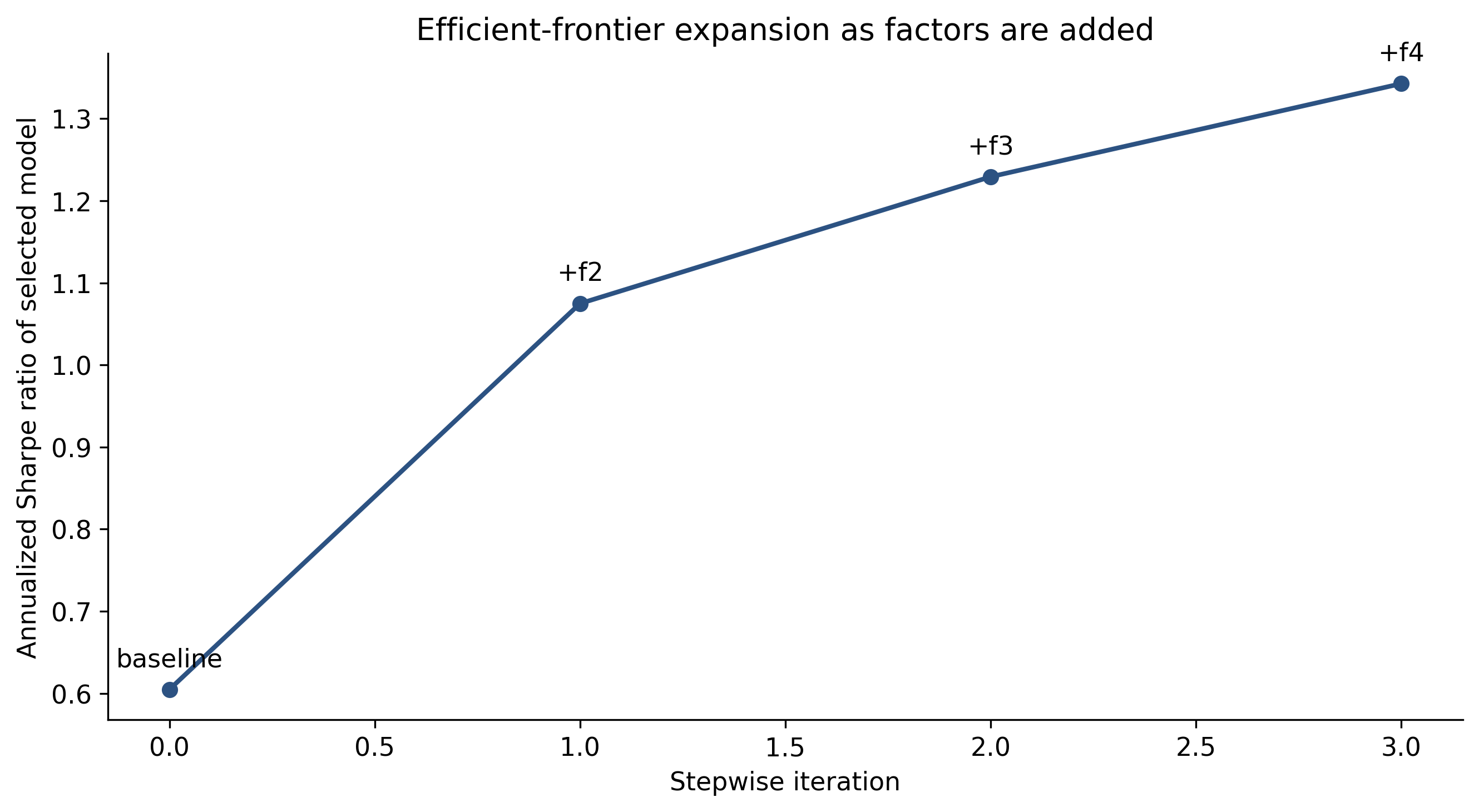
  +   f2  t(alpha)= 5.44  SR2_incr=0.0658  -> model SR2=0.096  Sharpe(ann)=1.07
  +   f3  t(alpha)= 3.58  SR2_incr=0.0296  -> model SR2=0.126  Sharpe(ann)=1.23
  +   f4  t(alpha)= 3.26  SR2_incr=0.0243  -> model SR2=0.150  Sharpe(ann)=1.34

Selected model : ['mkt', 'f2', 'f3', 'f4']
Final Sharpe   : 1.34 (annualized)
GRS on assets  : 0.33  p=0.998
Unselected candidates' spanning alphas (should be insignificant):
    r1: alpha_ann=-0.0053  t=-0.80  p=0.425
    r2: alpha_ann=-0.0104  t=-1.41  p=0.158
    d1: alpha_ann=+0.0195  t=+1.28  p=0.200
The procedure recovers exactly the true model ['mkt', 'f2', 'f3', 'f4']: it adds the three priced factors in order of their squared-Sharpe increment (each with a large, significant spanning \(t\)-statistic) and then halts, because every remaining candidate is now spanned. The two redundant factors and the decoy are left out, and their post-selection spanning alphas are small and insignificant—the model prices them, which is the property Feng et al. (2026) require of a valid model. The final GRS test on the test assets is comfortably non-rejected.
The economic content of the selection is the expansion of the efficient frontier, which we plot as the annualized Sharpe ratio of the selected model at each step.
Plot the frontier expansion across stepwise iterations
hist = pd.DataFrame(diag['history'])fig, ax = plt.subplots(figsize=(9, 5))ax.plot(range(len(hist)), hist['sharpe_ann'], 'o-', lw=2, color='#2C5282')for i, row in hist.iterrows(): ax.annotate(row['action'], (i, row['sharpe_ann']), textcoords='offset points', xytext=(0, 10), ha='center')ax.set_xlabel('Stepwise iteration')ax.set_ylabel('Annualized Sharpe ratio of selected model')ax.set_title('Efficient-frontier expansion as factors are added')plt.tight_layout()plt.show()
Figure 22.6: Efficient-frontier expansion under stepwise selection. Each point is the maximum annualized Sharpe ratio attainable from the model after that step; labels mark the factor added. The curve flattens as the added factors span progressively less of the residual frontier, and selection halts when no candidate improves it significantly.
22.8.4 Application to Vietnamese Factor Models
The procedure transfers directly to Vietnamese data: replace sim_factors with the locally constructed factor panel of Section 21.2 (market, size, value, profitability, investment, momentum, and any additional anomaly long-short returns that survive the multiple-testing screen of Section 21.4) and sim_test with a set of Vietnamese test portfolios (the size-BM and size-momentum sorts of Section 22.2). The baseline is the market factor; the candidate set is every anomaly factor with adequate coverage.
Stepwise selection on Vietnamese factors (real data)
# `factors` and the test-portfolio frames come from the DataCore pipeline# built earlier in this chapter (see the data-load chunk).vn_candidates = ['smb', 'hml', 'rmw', 'cma', 'wml'] # extend with local anomaliesvn_result = stepwise_select( factors=factors, candidate_cols=vn_candidates, baseline_cols=['mkt_excess'], test_assets=excess_25_bm, # 25 size-BM Vietnamese portfolios add_threshold=0.05/len(vn_candidates) # Bonferroni-style, see caveat below)print("Vietnamese stepwise model:", vn_result['selected'])print(f"GRS p-value: {vn_result['grs']['p_value']:.3f}")
Three caveats specific to the Vietnamese setting deserve emphasis, and each is a direct consequence of the market’s institutional features developed elsewhere in this book:
Short samples reduce power. Reliable Vietnamese factor data begins around 2008 (Section 22.2), giving fewer than 200 monthly observations. The spanning alpha \(t\)-statistics and the GRS test both lose power as \(T\) falls, so the procedure will tend to select smaller models than it would on the long US samples of Feng et al. (2026). A factor omitted on Vietnamese data is weakly priced given the available sample, not necessarily unpriced. Reporting the squared-Sharpe increment alongside the \(p\)-value (both are returned by the helpers above) keeps the economic magnitude visible even when statistical significance is marginal.
Correlated factors destabilize the path. Vietnamese value, quality, and profitability signals are empirically more collinear than in the US because they load on the same handful of large, state-linked firms. High collinearity inflates the residual variance in Equation 22.10 and makes the order of addition sensitive to the sample, so the selected model should be validated by re-running on bootstrap resamples (Section 21.7) and by checking out-of-sample stability (Section 21.8), not read off a single in-sample path.
Test-asset choice matters more in thin markets. With relatively few liquid stocks, finely partitioned test portfolios (for example 25 double sorts) contain noisy, thinly traded portfolios that can dominate the GRS statistic. Coarser sorts (\(2\times3\) or decile portfolios) and the price-limit-aware return construction of the microstructure chapter give more trustworthy stopping decisions.
Used with these caveats, the stepwise approach turns the sprawling Vietnamese factor zoo into a disciplined, testable model: rather than defaulting to an imported Fama-French specification, the researcher lets the local data select the factors that actually span the Vietnamese efficient frontier, and obtains an explicit pricing test of the result.
22.9 Conditional vs. Unconditional Tests
22.9.1 Time-Varying Betas
Unconditional tests assume constant betas. In practice, Vietnamese stock betas vary substantially over time due to changing market conditions, foreign ownership shifts, and sectoral rotations. We estimate rolling betas to assess the degree of time-variation:
Estimate and visualize time-varying betas
# Rolling 36-month betas for the 25 Size-BM portfolios on FF5rolling_window =36factor_cols = ['mkt_excess', 'smb', 'hml', 'rmw', 'cma']# Select a few representative portfoliosrepresentative = [excess_25_bm.columns[0], # Small-Growth excess_25_bm.columns[4], # Small-Value excess_25_bm.columns[20], # Big-Growth excess_25_bm.columns[24]] # Big-Valuerolling_betas = {}common = excess_25_bm.index.intersection(factors.index)for port in representative: betas_t = []for t inrange(rolling_window, len(common)): window = common[t - rolling_window:t] y = excess_25_bm.loc[window, port] X = sm.add_constant(factors.loc[window, factor_cols])try: model = sm.OLS(y, X).fit() entry = {'month': common[t]}for f in factor_cols: entry[f'beta_{f}'] = model.params[f] betas_t.append(entry)exceptException:pass rolling_betas[port] = pd.DataFrame(betas_t)
The analysis in this chapter yields the following guidelines for Vietnamese asset pricing research:
Use both approaches. Time-series tests (GRS) and cross-sectional tests (Fama-MacBeth) answer different questions. Always report both. If they disagree, investigate why rather than cherry-picking the more favorable result.
Be cautious with cross-sectional\(R^2\). High \(R^2\) from Fama-MacBeth on sorted portfolios is nearly guaranteed by the test asset structure. Always report the Lewellen, Nagel, and Shanken (2010) constrained \(R^2\) alongside the unconstrained value. Include industry portfolios as additional test assets.
Apply the Shanken correction. The EIV bias from estimated betas inflates Fama-MacBeth t-statistics. Always report Shanken-corrected standard errors for full-sample betas. For rolling betas, the correction is not straightforward, but the bias is smaller because beta estimation error averages out over time.
Use individual stocks with caution. Fama-MacBeth with individual stocks avoids the Lewellen-Nagel-Shanken critique but introduces severe noise: individual Vietnamese stocks are thin, volatile, and the monthly cross-section is small (500-700). The resulting risk premia will have wide confidence intervals. Report the average number of stocks per cross-section and the cross-sectional \(R^2\).
Examine conditional models. Rolling betas reveal substantial time-variation in Vietnamese stock exposures. If the research question is about risk compensation (does beta predict returns?), use rolling betas and control for time-variation. If the question is about model adequacy (do the factors span the mean-variance frontier?), full-sample betas and the GRS test are appropriate.
For model selection, use Barillas-Shanken. When comparing competing factor models (e.g., FF3 vs. FF5), the Barillas and Shanken (2018) approach (i.e., testing whether each model’s unique factors have alpha with respect to the other) is more informative than comparing GRS statistics on the same test assets.
22.11 Summary
Table 22.2: Summary of testing approaches for factor models.
Test
Question
Statistic
Strength
Weakness
TS regression (GRS)
Do all alphas = 0?
F-statistic
Clean null; joint test
Depends on test assets
Fama-MacBeth (portfolios)
Are betas priced?
\(\bar{\gamma}\), t-stat
Estimates risk premia
EIV bias; LNS critique
FM (individual stocks)
Are betas priced?
\(\bar{\gamma}\), t-stat
Avoids sorted portfolios
Noisy; small cross-section
LNS diagnostic
Is CS R² spurious?
Constrained R²
Reveals false positives
Only applicable to portfolios
GMM / SDF
Pricing errors jointly
J-stat, HJ distance
Flexible; model-free
Requires large N relative to K
Barillas-Shanken
Which model is better?
Alpha of unique factors
Model comparison
Requires traded factors
The gap between time-series and cross-sectional evidence is not a technicality—it reflects a fundamental ambiguity in what “a factor model works” means. In a market like Vietnam, where the cross-section is small, betas are time-varying, and test assets are inherently noisy, the two approaches will often disagree. The honest researcher reports both, investigates the source of disagreement, and treats any single test result with appropriate humility.
Barillas, Francisco, and Jay Shanken. 2018. “Comparing Asset Pricing Models.”The Journal of Finance 73 (2): 715–54.
Fama, Eugene F, and Kenneth R French. 2020. “Comparing Cross-Section and Time-Series Factor Models.”The Review of Financial Studies 33 (5): 1891–1926.
Fama, Eugene F, and James D MacBeth. 1973. “Risk, Return, and Equilibrium: Empirical Tests.”Journal of Political Economy 81 (3): 607–36.
Feng, Guanhao, Stefano Giglio, and Dacheng Xiu. 2020. “Taming the Factor Zoo: A Test of New Factors.”The Journal of Finance 75 (3): 1327–70.
Feng, Guanhao, Wei Lan, Hansheng Wang, and Jun Zhang. 2026. “Selecting and Testing Asset-Pricing Models: A Stepwise Approach.”Management Science. https://doi.org/10.1287/mnsc.2024.07804.
Gibbons, Michael R, Stephen A Ross, and Jay Shanken. 1989. “A Test of the Efficiency of a Given Portfolio.”Econometrica: Journal of the Econometric Society, 1121–52.
Goyal, Amit, and Narasimhan Jegadeesh. 2018. “Cross-Sectional and Time-Series Tests of Return Predictability: What Is the Difference?”The Review of Financial Studies 31 (5): 1784–824.
Hansen, Lars Peter. 1982. “Large Sample Properties of Generalized Method of Moments Estimators.”Econometrica: Journal of the Econometric Society, 1029–54.
Jagannathan, Ravi, and Zhenyu Wang. 1996. “The Conditional CAPM and the Cross-Section of Expected Returns.”The Journal of Finance 51 (1): 3–53.
Lewellen, Jonathan, Stefan Nagel, and Jay Shanken. 2010. “A Skeptical Appraisal of Asset Pricing Tests.”Journal of Financial Economics 96 (2): 175–94.
Pesaran, M Hashem, and Takashi Yamagata. 2024. “Testing for Alpha in Linear Factor Pricing Models with a Large Number of Securities.”Journal of Financial Econometrics 22 (2): 407–60.
Shanken, Jay. 1992. “On the Estimation of Beta-Pricing Models.”The Review of Financial Studies 5 (1): 1–33.
Source Code
# Time-Series vs. Cross-Sectional Factor Tests::: callout-noteIn this chapter, we implement and compare the two dominant approaches to testing asset pricing models: time-series regressions (do factors explain individual stock or portfolio returns?) and cross-sectional regressions (do factor exposures explain expected returns?), and develop the diagnostic tools to understand when and why they disagree.:::Every factor model makes two distinct claims. The **time-series claim** is that a set of factors explains the common variation in individual stock returns (i.e., when the factors move, stocks move with them in proportion to their exposures). The **cross-sectional claim** is that differences in average returns across stocks are explained by differences in their factor exposures (i.e., stocks that load more heavily on a factor earn higher (or lower) average returns in proportion to the factor's risk premium).These claims are logically related but empirically distinct. A factor can explain time-series variation without explaining the cross-section (if the factor's risk premium is zero, exposure to it creates no return differential). Conversely, a characteristic can predict the cross-section of returns without operating through a traded factor (if the characteristic captures mispricing rather than risk).@fama2020comparing formalize this distinction and show that the two approaches can give materially different answers about which factors matter. @goyal2018cross go further and demonstrate that time-series and cross-sectional tests can disagree about the same model (e.g., a factor can have a significant time-series alpha in one test and an insignificant cross-sectional premium in the other, or vice versa). Understanding *why* they disagree is essential for interpreting asset pricing evidence.This chapter equips the reader with both toolkits, applied to Vietnamese data, and develops the intuition for when each is appropriate.## The Two Testing Frameworks {#sec-ts-cs-framework}### Time-Series RegressionsThe time-series approach tests whether a factor model explains the returns of a set of test assets (typically portfolios). For each test asset $i$, estimate:$$R_{i,t} - R_{f,t} = \alpha_i + \beta_{i,1} f_{1,t} + \beta_{i,2} f_{2,t} + \ldots + \beta_{i,K} f_{K,t} + \varepsilon_{i,t}$$ {#eq-ts-regression}where $f_{k,t}$ are the $K$ factor returns. The intercept $\alpha_i$ measures the average return of asset $i$ that is *not* explained by the factors. Under the null that the model correctly prices asset $i$, $\alpha_i = 0$.The joint test of $H_0: \alpha_1 = \alpha_2 = \ldots = \alpha_N = 0$ across all $N$ test assets is performed using the @gibbons1989test (GRS) test statistic:$$\text{GRS} = \frac{T - N - K}{N} \cdot \frac{1}{1 + \bar{f}' \hat{\Sigma}_f^{-1} \bar{f}} \cdot \hat{\alpha}' \hat{\Sigma}_\varepsilon^{-1} \hat{\alpha} \sim F(N, T - N - K)$$ {#eq-grs}where $\bar{f}$ is the vector of factor means, $\hat{\Sigma}_f$ is the factor covariance matrix, and $\hat{\Sigma}_\varepsilon$ is the residual covariance matrix. A large GRS statistic rejects the model.### Cross-Sectional Regressions (Fama-MacBeth)The @fama1973risk cross-sectional approach tests whether factor exposures are priced (i.e., whether stocks with higher betas on a factor earn higher average returns). The procedure has two stages:**Stage 1 (Time-Series).** For each asset, estimate factor betas from a time-series regression over a rolling or full-sample window:$$R_{i,t} - R_{f,t} = \alpha_i + \beta_{i,1} f_{1,t} + \ldots + \beta_{i,K} f_{K,t} + \varepsilon_{i,t}$$ {#eq-fm-stage1}**Stage 2 (Cross-Section).** Each month $t$, regress the cross-section of realized excess returns on the estimated betas:$$R_{i,t} - R_{f,t} = \gamma_{0,t} + \gamma_{1,t} \hat{\beta}_{i,1} + \ldots + \gamma_{K,t} \hat{\beta}_{i,K} + \eta_{i,t}$$ {#eq-fm-stage2}The time-series averages $\bar{\gamma}_k = \frac{1}{T} \sum_t \gamma_{k,t}$ estimate the risk premia, and the standard errors use the time-series standard deviation of $\{\gamma_{k,t}\}$.### Key Differences| Dimension | Time-Series | Cross-Section ||------------------------|------------------------|------------------------|| What it tests | Do factors explain return variation? | Do factor exposures explain average returns? || Key statistic | Alpha (intercept) | Risk premium ($\gamma$) || Joint test | GRS F-test | Chi-squared on $\gamma$'s || Test assets | Portfolios (usually) | Individual stocks or portfolios || Factors | Must be traded returns | Can be non-traded (macro, characteristics) || Null hypothesis | $\alpha_i = 0$ for all $i$ | $\gamma_k$ equals factor mean return || Errors-in-variables | Not an issue (factors observed) | Estimated betas create EIV bias |: Comparison of time-series and cross-sectional testing frameworks. {#tbl-ts-cs-comparison}## Data Construction {#sec-ts-cs-data}```{python}#| label: setup#| code-summary: "Import libraries and configure environment"import pandas as pdimport numpy as npimport matplotlib.pyplot as pltimport seaborn as snsimport statsmodels.api as smfrom scipy import statsfrom scipy.linalg import invimport warningswarnings.filterwarnings('ignore')plt.rcParams.update({'figure.figsize': (12, 6),'figure.dpi': 150,'font.size': 11,'axes.spines.top': False,'axes.spines.right': False})``````{python}#| label: data-load#| eval: false#| code-summary: "Load factor returns, test portfolios, and individual stock data"from datacore import DataCoreClientclient = DataCoreClient()# Factor returnsfactors = client.get_factor_returns( market='vietnam', start_date='2008-01-01', end_date='2024-12-31', factors=['mkt_excess', 'smb', 'hml', 'rmw', 'cma', 'wml'])factors['month_end'] = pd.to_datetime(factors['month_end'])factors = factors.set_index('month_end')# Test portfolios: 25 size-BM portfolios (5x5 independent sorts)test_portfolios_25 = client.get_sorted_portfolios( market='vietnam', sort_vars=['size', 'bm'], n_groups=[5, 5], start_date='2008-01-01', end_date='2024-12-31', weighting='value')# Test portfolios: 25 size-momentum portfoliostest_portfolios_mom = client.get_sorted_portfolios( market='vietnam', sort_vars=['size', 'momentum_12_2'], n_groups=[5, 5], start_date='2008-01-01', end_date='2024-12-31', weighting='value')# Test portfolios: 10 industry portfoliostest_portfolios_ind = client.get_sorted_portfolios( market='vietnam', sort_vars=['icb_sector'], n_groups=[10], start_date='2008-01-01', end_date='2024-12-31', weighting='value')# Monthly individual stock returns for Fama-MacBethstock_returns = client.get_monthly_returns( exchanges=['HOSE', 'HNX'], start_date='2008-01-01', end_date='2024-12-31', include_delisted=True, fields=['ticker', 'month_end', 'monthly_return', 'market_cap'])# Risk-free raterf = client.get_risk_free_rate( start_date='2008-01-01', end_date='2024-12-31', frequency='monthly')print(f"Factor months: {len(factors)}")print(f"25 Size-BM portfolios: {test_portfolios_25.shape}")print(f"25 Size-Mom portfolios: {test_portfolios_mom.shape}")print(f"10 Industry portfolios: {test_portfolios_ind.shape}")print(f"Stock-months: {len(stock_returns):,}")``````{python}#| label: prepare-test-assets#| eval: false#| code-summary: "Prepare excess return matrices for test portfolios"# Convert test portfolios to excess returns# Each portfolio set is a DataFrame: rows = months, columns = portfoliosdef prepare_test_assets(port_df, rf_df):"""Convert portfolio returns to excess returns matrix.""" port = port_df.set_index('month_end') rf_aligned = rf_df.set_index('month_end')['rf'].reindex(port.index) excess = port.subtract(rf_aligned, axis=0)return excess.dropna()excess_25_bm = prepare_test_assets(test_portfolios_25, rf)excess_25_mom = prepare_test_assets(test_portfolios_mom, rf)excess_10_ind = prepare_test_assets(test_portfolios_ind, rf)print(f"Size-BM test assets: {excess_25_bm.shape[1]} portfolios, "f"{excess_25_bm.shape[0]} months")print(f"Size-Mom test assets: {excess_25_mom.shape[1]} portfolios, "f"{excess_25_mom.shape[0]} months")print(f"Industry test assets: {excess_10_ind.shape[1]} portfolios, "f"{excess_10_ind.shape[0]} months")```## Time-Series Tests {#sec-ts-cs-ts-tests}### Full-Sample Time-Series RegressionsWe begin by running full-sample time-series regressions of each test portfolio on the Fama-French five-factor model plus momentum:```{python}#| label: ts-regressions#| eval: false#| code-summary: "Run time-series regressions for all test portfolios"def time_series_regressions(excess_returns, factor_df, factor_cols, cov_type='HAC', maxlags=6):""" Run time-series regressions of test assets on factors. Returns DataFrame of alphas, betas, t-stats, and R-squared. """# Align dates common = excess_returns.index.intersection(factor_df.index) Y = excess_returns.loc[common] X = factor_df.loc[common, factor_cols] X_const = sm.add_constant(X) results = {}for col in Y.columns: y = Y[col].dropna() x = X_const.loc[y.index] model = sm.OLS(y, x).fit( cov_type=cov_type, cov_kwds={'maxlags': maxlags} if cov_type =='HAC'else {} ) result = {'alpha': model.params['const'],'alpha_t': model.tvalues['const'],'alpha_p': model.pvalues['const'],'r_squared': model.rsquared,'r_squared_adj': model.rsquared_adj }for f in factor_cols: result[f'beta_{f}'] = model.params[f] result[f't_{f}'] = model.tvalues[f] results[col] = resultreturn pd.DataFrame(results).T# Define models to testmodels = {'CAPM': ['mkt_excess'],'FF3': ['mkt_excess', 'smb', 'hml'],'FF5': ['mkt_excess', 'smb', 'hml', 'rmw', 'cma'],'FF5+WML': ['mkt_excess', 'smb', 'hml', 'rmw', 'cma', 'wml'],}# Run for 25 Size-BM portfoliosprint("Time-Series Alphas: 25 Size-BM Portfolios")print("="*60)ts_results = {}for model_name, factor_cols in models.items(): result = time_series_regressions( excess_25_bm, factors, factor_cols ) ts_results[model_name] = result mean_alpha = result['alpha'].mean() *12 mean_abs_alpha = result['alpha'].abs().mean() *12 pct_sig = (result['alpha_p'] <0.05).mean() mean_r2 = result['r_squared'].mean()print(f"\n{model_name}:")print(f" Mean alpha (ann.): {mean_alpha:.4f}")print(f" Mean |alpha| (ann.): {mean_abs_alpha:.4f}")print(f" % sig. at 5%: {pct_sig:.1%}")print(f" Mean R²: {mean_r2:.3f}")```### The GRS Test```{python}#| label: grs-test#| eval: false#| code-summary: "Implement and compute the GRS test statistic"def grs_test(excess_returns, factor_df, factor_cols):""" Gibbons, Ross, Shanken (1989) test of H0: all alphas = 0. Returns GRS statistic, p-value, and related diagnostics. """ common = excess_returns.index.intersection(factor_df.index) Y = excess_returns.loc[common].values # T x N F = factor_df.loc[common, factor_cols].values # T x K T, N = Y.shape K = F.shape[1]# Add constant and run OLS for each asset F_const = np.column_stack([np.ones(T), F])# OLS: beta = (X'X)^-1 X'Y XtX_inv = inv(F_const.T @ F_const) B = XtX_inv @ F_const.T @ Y # (K+1) x N alpha = B[0, :] # N-vector of intercepts residuals = Y - F_const @ B # T x N# Residual covariance matrix Sigma_eps = residuals.T @ residuals / (T - K -1)# Factor mean and covariance f_bar = F.mean(axis=0) Sigma_f = np.cov(F, rowvar=False, ddof=1)# GRS statistic Sigma_eps_inv = inv(Sigma_eps) Sigma_f_inv = inv(Sigma_f) if K >1else np.array([[1/ Sigma_f]]) sharpe_sq_alpha = alpha @ Sigma_eps_inv @ alpha sharpe_sq_f = f_bar @ Sigma_f_inv @ f_bar if K >1else (f_bar[0] **2/ Sigma_f) grs_stat = ((T - N - K) / N) * (1/ (1+ sharpe_sq_f)) * sharpe_sq_alpha# p-value from F distribution p_value =1- stats.f.cdf(grs_stat, N, T - N - K)# Additional diagnostics# Sharpe ratio of tangency portfolio of factors sr_factors = np.sqrt(sharpe_sq_f)# Sharpe ratio of tangency portfolio including alphas sr_alpha = np.sqrt(sharpe_sq_alpha + sharpe_sq_f)return {'GRS': grs_stat,'p_value': p_value,'df1': N,'df2': T - N - K,'mean_abs_alpha': np.abs(alpha).mean(),'sr_factors': sr_factors,'sr_alpha_plus_factors': sr_alpha,'sr_improvement': sr_alpha - sr_factors,'T': T, 'N': N, 'K': K }# Run GRS for each model on each set of test assetsprint("GRS Test Results")print("="*80)print(f"{'Model':<12}{'Test Assets':<18}{'GRS':>8}{'p-value':>10} "f"{'|α| ann':>10}{'SR(f)':>8}{'SR(α+f)':>8}")print("-"*80)test_asset_sets = {'25 Size-BM': excess_25_bm,'25 Size-Mom': excess_25_mom,'10 Industry': excess_10_ind}grs_all = {}for model_name, factor_cols in models.items():for ta_name, ta_data in test_asset_sets.items(): key =f"{model_name}_{ta_name}" result = grs_test(ta_data, factors, factor_cols) grs_all[key] = resultprint(f"{model_name:<12}{ta_name:<18} "f"{result['GRS']:>8.2f}{result['p_value']:>10.4f} "f"{result['mean_abs_alpha']*12:>10.4f} "f"{result['sr_factors']:>8.3f} "f"{result['sr_alpha_plus_factors']:>8.3f}")``````{python}#| label: fig-alpha-patterns#| eval: false#| fig-cap: "Time-series alphas from the Fama-French five-factor model for the 25 size-BM portfolios. Each cell represents a portfolio formed by independently sorting on size (rows, small to big) and book-to-market (columns, growth to value). Significant alphas (|t| > 2) are marked with asterisks. Systematic patterns in the alpha matrix reveal dimensions of expected returns that the model fails to capture."#| code-summary: "Plot the alpha matrix for Size-BM portfolios"ff5_result = ts_results['FF5']# Reshape alphas into 5x5 matrixalpha_matrix = ff5_result['alpha'].values.reshape(5, 5) *12*100t_matrix = ff5_result['alpha_t'].values.reshape(5, 5)fig, axes = plt.subplots(1, 2, figsize=(14, 5))# Panel A: Alpha magnitudesim = axes[0].imshow(alpha_matrix, cmap='RdBu_r', aspect='auto', vmin=-np.max(np.abs(alpha_matrix)), vmax=np.max(np.abs(alpha_matrix)))for i inrange(5):for j inrange(5): sig ='*'ifabs(t_matrix[i, j]) >2else'' axes[0].text(j, i, f'{alpha_matrix[i, j]:.1f}{sig}', ha='center', va='center', fontsize=9, color='white'ifabs(alpha_matrix[i, j]) >3else'black')axes[0].set_xticks(range(5))axes[0].set_xticklabels(['Growth', '2', '3', '4', 'Value'])axes[0].set_yticks(range(5))axes[0].set_yticklabels(['Small', '2', '3', '4', 'Big'])axes[0].set_xlabel('Book-to-Market')axes[0].set_ylabel('Size')axes[0].set_title('Panel A: FF5 Alphas (% ann.)')plt.colorbar(im, ax=axes[0], label='Alpha (% ann.)')# Panel B: R-squaredr2_matrix = ff5_result['r_squared'].values.reshape(5, 5) *100im2 = axes[1].imshow(r2_matrix, cmap='YlGn', aspect='auto', vmin=50, vmax=100)for i inrange(5):for j inrange(5): axes[1].text(j, i, f'{r2_matrix[i, j]:.0f}%', ha='center', va='center', fontsize=9)axes[1].set_xticks(range(5))axes[1].set_xticklabels(['Growth', '2', '3', '4', 'Value'])axes[1].set_yticks(range(5))axes[1].set_yticklabels(['Small', '2', '3', '4', 'Big'])axes[1].set_xlabel('Book-to-Market')axes[1].set_ylabel('Size')axes[1].set_title('Panel B: R-squared (%)')plt.colorbar(im2, ax=axes[1], label='R² (%)')plt.tight_layout()plt.show()```### Model Comparison via GRS```{python}#| label: fig-grs-comparison#| eval: false#| fig-cap: "GRS test statistics across models and test asset sets. Lower GRS values indicate better model performance (fewer unexplained pricing errors). The FF5+WML model generally produces the lowest GRS, but no model fully prices all test asset sets—consistent with the U.S. evidence that no existing model eliminates all alphas."#| code-summary: "Visualize GRS statistics across models and test assets"fig, ax = plt.subplots(figsize=(12, 5))model_names =list(models.keys())ta_names =list(test_asset_sets.keys())x = np.arange(len(model_names))width =0.25colors_ta = ['#2C5F8A', '#C0392B', '#27AE60']for i, ta_name inenumerate(ta_names): grs_vals = [grs_all[f"{m}_{ta_name}"]['GRS'] for m in model_names] bars = ax.bar(x + i * width, grs_vals, width, alpha=0.85, color=colors_ta[i], label=ta_name, edgecolor='white')ax.set_xticks(x + width)ax.set_xticklabels(model_names)ax.set_ylabel('GRS Statistic')ax.set_title('GRS Test: Model Comparison Across Test Asset Sets')ax.legend()# Add critical value line (5% significance)# Approximate: depends on N, T, Kax.axhline(y=1.8, color='gray', linestyle='--', linewidth=1, label='~5% critical value')plt.tight_layout()plt.show()```## Cross-Sectional Tests {#sec-ts-cs-cs-tests}### Fama-MacBeth with Portfolio Test AssetsWe implement the Fama-MacBeth two-pass procedure using the 25 size-BM portfolios as test assets:```{python}#| label: fama-macbeth-portfolios#| eval: false#| code-summary: "Full Fama-MacBeth two-pass procedure on portfolio test assets"def fama_macbeth_two_pass(excess_returns, factor_df, factor_cols, beta_window='full', rolling_window=60, shanken_correction=True):""" Fama-MacBeth (1973) two-pass cross-sectional regression. Parameters ---------- beta_window : str 'full' for full-sample betas, 'rolling' for rolling betas. shanken_correction : bool Apply Shanken (1992) errors-in-variables correction. Returns ------- Dictionary with estimated risk premia, t-statistics, and diagnostics. """ common = excess_returns.index.intersection(factor_df.index) Y = excess_returns.loc[common] F = factor_df.loc[common, factor_cols] T =len(common) N = Y.shape[1] K =len(factor_cols) months =sorted(common)# ===== STAGE 1: Estimate betas =====if beta_window =='full':# Full-sample betas (simpler, used in GRS context) F_const = sm.add_constant(F) betas = {}for col in Y.columns: model = sm.OLS(Y[col], F_const).fit() betas[col] = {f: model.params[f] for f in factor_cols} beta_df = pd.DataFrame(betas).T # N x K# Same betas used every month beta_by_month = {m: beta_df for m in months}elif beta_window =='rolling':# Rolling betas (more realistic, avoids look-ahead) beta_by_month = {}for t_idx inrange(rolling_window, T): month = months[t_idx] window_start = months[t_idx - rolling_window] Y_win = Y.loc[window_start:months[t_idx -1]] F_win = sm.add_constant(F.loc[window_start:months[t_idx -1]]) betas_t = {}for col in Y.columns: y = Y_win[col].dropna() x = F_win.loc[y.index]iflen(y) <24: betas_t[col] = {f: np.nan for f in factor_cols}continue model = sm.OLS(y, x).fit() betas_t[col] = {f: model.params[f] for f in factor_cols} beta_by_month[month] = pd.DataFrame(betas_t).T# ===== STAGE 2: Cross-sectional regressions ===== gamma_list = []for month in months:if month notin beta_by_month:continue betas_t = beta_by_month[month] returns_t = Y.loc[month]# Align valid = betas_t.dropna().index.intersection(returns_t.dropna().index)iflen(valid) < K +5:continue y = returns_t[valid].values X = sm.add_constant(betas_t.loc[valid, factor_cols].values)try: model = sm.OLS(y, X).fit() gammas = {'month': month, 'gamma_0': model.params[0]}for j, f inenumerate(factor_cols): gammas[f'gamma_{f}'] = model.params[j +1] gammas['r_squared'] = model.rsquared gammas['n_assets'] =len(valid) gamma_list.append(gammas)exceptException:pass gamma_df = pd.DataFrame(gamma_list)iflen(gamma_df) ==0:returnNone# ===== INFERENCE =====# Time-series averages of gammas gamma_cols = ['gamma_0'] + [f'gamma_{f}'for f in factor_cols] results = {}for col in gamma_cols: g = gamma_df[col] mean = g.mean() se_fm = g.std() / np.sqrt(len(g)) t_fm = mean / se_fm if se_fm >0else np.nan results[col] = {'estimate': mean,'se_fm': se_fm,'t_fm': t_fm, }# Shanken (1992) correction for errors-in-variablesif shanken_correction and beta_window =='full': Sigma_f = F[factor_cols].cov().values# Shanken correction factor: (1 + lambda' Sigma_f^-1 lambda) gamma_factor = np.array([results[f'gamma_{f}']['estimate']for f in factor_cols])try: Sigma_f_inv = inv(Sigma_f) c_shanken =1+ gamma_factor @ Sigma_f_inv @ gamma_factorexceptException: c_shanken =1.0for col in gamma_cols: results[col]['se_shanken'] = results[col]['se_fm'] * np.sqrt(c_shanken) results[col]['t_shanken'] = (results[col]['estimate']/ results[col]['se_shanken']if results[col]['se_shanken'] >0else np.nan)# Compare estimated premia to factor mean returns factor_means = F[factor_cols].mean()for f in factor_cols: results[f'gamma_{f}']['factor_mean'] = factor_means[f]# Cross-sectional R-squared results['avg_cs_r2'] = gamma_df['r_squared'].mean()return {'results': pd.DataFrame(results).T,'gamma_ts': gamma_df,'beta_df': beta_by_month.get(months[-1], None) }# Run Fama-MacBeth for each modelprint("Fama-MacBeth Cross-Sectional Results: 25 Size-BM Portfolios")print("="*80)fm_results = {}for model_name, factor_cols in models.items():for beta_type in ['full', 'rolling']: key =f"{model_name}_{beta_type}" fm = fama_macbeth_two_pass( excess_25_bm, factors, factor_cols, beta_window=beta_type, rolling_window=60, shanken_correction=(beta_type =='full') )if fm isNone:continue fm_results[key] = fmprint(f"\n{model_name} (betas: {beta_type}):") res = fm['results']for idx, row in res.iterrows():if'gamma'in idx: t_col ='t_shanken'if't_shanken'in row and pd.notna(row.get('t_shanken')) else't_fm' f_mean = row.get('factor_mean', '') f_str =f" f_mean={f_mean:.4f}"ifisinstance(f_mean, float) else""print(f" {idx:<16}: γ = {row['estimate']:.5f}, "f"t = {row[t_col]:.2f}{f_str}")if'avg_cs_r2'in res.index:print(f" Avg CS R²: {res.loc['avg_cs_r2', 'estimate']:.3f}")```### The Shanken CorrectionThe @shanken1992estimation correction addresses the errors-in-variables (EIV) problem inherent in the two-pass procedure. Because betas are estimated with error in Stage 1, the Stage 2 standard errors are understated. The correction inflates the standard errors by a factor that depends on the estimated risk premia and the factor covariance matrix:$$\text{Var}(\hat{\gamma})_{\text{Shanken}} = \text{Var}(\hat{\gamma})_{\text{FM}} \times \left(1 + \hat{\gamma}' \hat{\Sigma}_f^{-1} \hat{\gamma}\right)$$ {#eq-shanken}```{python}#| label: shanken-impact#| eval: false#| code-summary: "Compare FM t-statistics with and without Shanken correction"print("Impact of Shanken Correction on t-statistics:")print(f"{'Model':<12}{'Factor':<12}{'t (FM)':>10}{'t (Shanken)':>12}{'Ratio':>8}")print("-"*54)for model_name in models: key =f"{model_name}_full"if key notin fm_results:continue res = fm_results[key]['results']for idx, row in res.iterrows():if'gamma_'instr(idx) and idx !='gamma_0': t_fm = row.get('t_fm', np.nan) t_sh = row.get('t_shanken', np.nan) ratio = t_fm / t_sh if pd.notna(t_sh) and t_sh !=0else np.nan factor_name = idx.replace('gamma_', '')print(f"{model_name:<12}{factor_name:<12}{t_fm:>10.2f} "f"{t_sh:>12.2f}{ratio:>8.2f}")```### Fama-MacBeth with Individual StocksUsing individual stocks instead of portfolios as test assets avoids the @lewellen2010skeptical critique that sorted portfolios create artificially strong factor structure:```{python}#| label: fm-individual#| eval: false#| code-summary: "Fama-MacBeth regressions using individual stocks"def fama_macbeth_individual(stock_df, factor_df, factor_cols, beta_window=60, min_obs=36, min_stocks=100):""" Fama-MacBeth with individual stocks and rolling betas. """ stock_df = stock_df.copy() stock_df['month_end'] = pd.to_datetime(stock_df['month_end']) factor_df = factor_df.copy() months =sorted(stock_df['month_end'].unique())# Pre-compute rolling betas for all stocks gamma_list = []for t_idx, month inenumerate(months):if t_idx < beta_window:continue window_months = months[t_idx - beta_window:t_idx]# Get betas for each stock from rolling window betas_t = {} window_data = stock_df[stock_df['month_end'].isin(window_months)]for ticker, group in window_data.groupby('ticker'):iflen(group) < min_obs:continue y = group.set_index('month_end')['monthly_return'] x = factor_df.loc[y.index, factor_cols] x = sm.add_constant(x) valid = y.index.intersection(x.index)iflen(valid) < min_obs:continuetry: model = sm.OLS(y[valid], x.loc[valid]).fit() betas_t[ticker] = {f: model.params[f] for f in factor_cols}exceptException:passiflen(betas_t) < min_stocks:continue beta_df = pd.DataFrame(betas_t).T# Current month returns current = stock_df[stock_df['month_end'] == month] current = current.set_index('ticker')# Align valid_tickers = beta_df.index.intersection(current.index)iflen(valid_tickers) < min_stocks:continue y = current.loc[valid_tickers, 'monthly_return'].values X = sm.add_constant(beta_df.loc[valid_tickers].values)try: model = sm.OLS(y, X).fit() gammas = {'month': month, 'gamma_0': model.params[0]}for j, f inenumerate(factor_cols): gammas[f'gamma_{f}'] = model.params[j +1] gammas['n_stocks'] =len(valid_tickers) gammas['r_squared'] = model.rsquared gamma_list.append(gammas)exceptException:pass gamma_df = pd.DataFrame(gamma_list)# Inference gamma_cols = ['gamma_0'] + [f'gamma_{f}'for f in factor_cols] summary = {}for col in gamma_cols: g = gamma_df[col] mean = g.mean() se = g.std() / np.sqrt(len(g)) t = mean / se if se >0else np.nan summary[col] = {'estimate': mean, 'se': se, 't': t} summary['avg_n_stocks'] = gamma_df['n_stocks'].mean() summary['avg_cs_r2'] = gamma_df['r_squared'].mean()return pd.DataFrame(summary).T, gamma_df# Run for FF5print("\nFama-MacBeth with Individual Stocks (FF5):")fm_ind_results, fm_ind_gamma = fama_macbeth_individual( stock_returns, factors, ['mkt_excess', 'smb', 'hml', 'rmw', 'cma'], beta_window=60, min_obs=36)print(fm_ind_results.round(4).to_string())```## When Do the Tests Disagree? {#sec-ts-cs-disagreement}### Theoretical Sources of Disagreement@goyal2018cross identify three sources of discrepancy between time-series and cross-sectional tests:**1. Factor structure of test assets.** If test assets have a strong factor structure (as sorted portfolios do by construction), the cross-sectional $R^2$ will be high regardless of whether the factors truly price the assets. @lewellen2010skeptical show that even random factors can achieve high cross-sectional $R^2$ when test assets are size-BM sorted portfolios, because such portfolios have a strong linear structure in the size-value space.**2. Time-variation in betas.** The time-series regression assumes constant betas. If betas vary over time and co-move with the factor risk premium, the unconditional time-series alpha can be nonzero even if the conditional model holds [@jagannathan1996conditional].**3. Misspecified risk premia.** The Fama-MacBeth cross-sectional regression estimates the risk premium from the data. The time-series regression implicitly sets the risk premium equal to the factor's sample mean return. When these differ (e.g., because the factor is not a perfect proxy for the underlying risk), the two approaches disagree.### Empirical Comparison for Vietnam```{python}#| label: ts-vs-cs#| eval: false#| code-summary: "Compare time-series alphas with cross-sectional pricing errors"# For FF5 on 25 Size-BM portfolios:# Time-series: alpha from OLS regression# Cross-section: pricing error from Fama-MacBethts_alphas = ts_results['FF5']['alpha'].values *12# Annualizedts_names = ts_results['FF5'].index.tolist()# Cross-sectional pricing errors:# Predicted return = beta' * estimated_gamma# Pricing error = actual mean return - predictedfm_full = fm_results.get('FF5_full')if fm_full: betas = fm_full['beta_df'] # N x K factor_cols = ['mkt_excess', 'smb', 'hml', 'rmw', 'cma'] gammas = np.array([fm_full['results'].loc[f'gamma_{f}', 'estimate']for f in factor_cols]) gamma_0 = fm_full['results'].loc['gamma_0', 'estimate'] actual_means = excess_25_bm.mean() *12# Annualized predicted = (gamma_0 + betas[factor_cols].values @ gammas) *12 cs_errors = actual_means.values - predicted``````{python}#| label: fig-ts-vs-cs#| eval: false#| fig-cap: "Comparison of time-series alphas and cross-sectional pricing errors for the 25 size-BM portfolios under the FF5 model. Panel A plots the two measures against each other; perfect agreement would place all points on the 45-degree line. Panel B shows actual vs predicted average returns from the Fama-MacBeth second pass. Systematic deviations reveal where the two approaches disagree about model adequacy."#| code-summary: "Scatter plot comparing TS alphas and CS pricing errors"fig, axes = plt.subplots(1, 2, figsize=(14, 5))# Panel A: TS alpha vs CS pricing errorif fm_full: axes[0].scatter(ts_alphas *100, cs_errors *100, color='#2C5F8A', s=60, alpha=0.7, edgecolors='white') lim =max(np.max(np.abs(ts_alphas)), np.max(np.abs(cs_errors))) *100+1 axes[0].plot([-lim, lim], [-lim, lim], 'k--', linewidth=1) axes[0].plot([-lim, lim], [0, 0], color='gray', linewidth=0.5) axes[0].plot([0, 0], [-lim, lim], color='gray', linewidth=0.5) axes[0].set_xlabel('Time-Series Alpha (% ann.)') axes[0].set_ylabel('Cross-Sectional Pricing Error (% ann.)') axes[0].set_title('Panel A: TS Alpha vs CS Pricing Error')# Correlation rho = np.corrcoef(ts_alphas, cs_errors)[0, 1] axes[0].text(0.05, 0.95, f'ρ = {rho:.2f}', transform=axes[0].transAxes, fontsize=11)# Panel B: Actual vs Predicted (CS)if fm_full: axes[1].scatter(predicted *100, actual_means.values *100, color='#C0392B', s=60, alpha=0.7, edgecolors='white') lim2 =max(np.max(np.abs(predicted)), np.max(np.abs(actual_means))) *100+2 axes[1].plot([-5, lim2], [-5, lim2], 'k--', linewidth=1) axes[1].set_xlabel('Predicted Average Return (% ann.)') axes[1].set_ylabel('Actual Average Return (% ann.)') axes[1].set_title('Panel B: Actual vs Predicted (FM Cross-Section)')# CS R-squared ss_res = np.sum((actual_means.values - predicted) **2) ss_tot = np.sum((actual_means.values - actual_means.values.mean()) **2) r2_cs =1- ss_res / ss_tot axes[1].text(0.05, 0.95, f'CS R² = {r2_cs:.2f}', transform=axes[1].transAxes, fontsize=11)plt.tight_layout()plt.show()```### The Lewellen-Nagel-Shanken Critique@lewellen2010skeptical demonstrate that the high cross-sectional $R^2$ from Fama-MacBeth regressions on sorted portfolios can be misleading. Sorted portfolios have a strong factor structure by construction, so even irrelevant factors can produce high $R^2$. They recommend:1. Including industry portfolios alongside sorted portfolios to break the mechanical factor structure.2. Constraining the estimated risk premia to equal the factor mean returns (this is what the time-series test implicitly does).3. Reporting the cross-sectional $R^2$ from the *constrained* model alongside the unconstrained estimate.```{python}#| label: lns-critique#| eval: false#| code-summary: "Implement the Lewellen-Nagel-Shanken diagnostic"def lns_diagnostic(excess_returns, factor_df, factor_cols):""" Lewellen-Nagel-Shanken (2010) diagnostic: Compare unconstrained CS R² to constrained (factor mean = premium). """ common = excess_returns.index.intersection(factor_df.index) Y = excess_returns.loc[common] F = factor_df.loc[common, factor_cols]# Full-sample betas betas = {} F_const = sm.add_constant(F)for col in Y.columns: model = sm.OLS(Y[col], F_const).fit() betas[col] = {f: model.params[f] for f in factor_cols} beta_mat = pd.DataFrame(betas).T # N x K actual = Y.mean() *12# Annualized# Unconstrained: FM regression X = sm.add_constant(beta_mat.values) fm_model = sm.OLS(actual.values, X).fit() predicted_unc = fm_model.fittedvalues r2_unconstrained = fm_model.rsquared# Constrained: premium = factor mean return factor_means = F.mean().values *12# Annualized predicted_con = beta_mat.values @ factor_means# Add best-fitting intercept intercept_con = np.mean(actual.values - predicted_con) predicted_con += intercept_con ss_res_con = np.sum((actual.values - predicted_con) **2) ss_tot = np.sum((actual.values - actual.values.mean()) **2) r2_constrained =1- ss_res_con / ss_totreturn {'r2_unconstrained': r2_unconstrained,'r2_constrained': r2_constrained,'r2_drop': r2_unconstrained - r2_constrained,'gamma_unconstrained': fm_model.params[1:],'gamma_constrained': factor_means }print("Lewellen-Nagel-Shanken Diagnostic:")print(f"{'Model':<12}{'Test Assets':<18}{'R² (unc)':>10}{'R² (con)':>10} "f"{'Drop':>8}")print("-"*58)for model_name, factor_cols in models.items():for ta_name, ta_data in test_asset_sets.items(): diag = lns_diagnostic(ta_data, factors, factor_cols)print(f"{model_name:<12}{ta_name:<18} "f"{diag['r2_unconstrained']:>10.3f} "f"{diag['r2_constrained']:>10.3f} "f"{diag['r2_drop']:>8.3f}")``````{python}#| label: fig-lns#| eval: false#| fig-cap: "Lewellen-Nagel-Shanken diagnostic for the FF5 model. Panel A shows the unconstrained cross-sectional fit (estimated risk premia), where high R² may be spurious. Panel B shows the constrained fit (premia set to factor means). A large drop in R² from unconstrained to constrained indicates that the model's apparent success relies on implausible risk premia, and the factors are not truly pricing the test assets."#| code-summary: "Visualize constrained vs unconstrained cross-sectional fit"diag_ff5 = lns_diagnostic(excess_25_bm, factors, ['mkt_excess', 'smb', 'hml', 'rmw', 'cma'])fig, axes = plt.subplots(1, 2, figsize=(14, 5))actual = excess_25_bm.mean().values *12*100# Panel A: UnconstrainedF_const = sm.add_constant(factors[['mkt_excess', 'smb', 'hml', 'rmw', 'cma']])betas_full = {}for col in excess_25_bm.columns: common = excess_25_bm.index.intersection(factors.index) model = sm.OLS(excess_25_bm.loc[common, col], F_const.loc[common]).fit() betas_full[col] = {f: model.params[f] for f in ['mkt_excess', 'smb', 'hml', 'rmw', 'cma']}beta_mat = pd.DataFrame(betas_full).TX_cs = sm.add_constant(beta_mat.values)fm_mod = sm.OLS(actual, X_cs).fit()pred_unc = fm_mod.fittedvaluesaxes[0].scatter(pred_unc, actual, color='#2C5F8A', s=60, alpha=0.7, edgecolors='white')rng_plot = [min(pred_unc.min(), actual.min()) -1,max(pred_unc.max(), actual.max()) +1]axes[0].plot(rng_plot, rng_plot, 'k--', linewidth=1)axes[0].set_xlabel('Predicted (% ann.)')axes[0].set_ylabel('Actual (% ann.)')axes[0].set_title(f"Panel A: Unconstrained (R² = "f"{diag_ff5['r2_unconstrained']:.2f})")# Panel B: Constrainedfactor_means = factors[['mkt_excess', 'smb', 'hml', 'rmw', 'cma']].mean().values *12*100pred_con = beta_mat.values @ factor_meanspred_con += np.mean(actual - pred_con)axes[1].scatter(pred_con, actual, color='#C0392B', s=60, alpha=0.7, edgecolors='white')rng2 = [min(pred_con.min(), actual.min()) -1,max(pred_con.max(), actual.max()) +1]axes[1].plot(rng2, rng2, 'k--', linewidth=1)axes[1].set_xlabel('Predicted (% ann.)')axes[1].set_ylabel('Actual (% ann.)')axes[1].set_title(f"Panel B: Constrained (R² = "f"{diag_ff5['r2_constrained']:.2f})")plt.tight_layout()plt.show()```## GMM-Based Tests {#sec-ts-cs-gmm}### The Stochastic Discount Factor FrameworkBoth time-series and cross-sectional tests are special cases of the @hansen1982large Generalized Method of Moments (GMM) framework. The fundamental pricing equation is:$$E[M_t R_{i,t}^e] = 0 \quad \text{for all } i$$ {#eq-sdf}where $M_t$ is the stochastic discount factor (SDF) and $R_{i,t}^e$ is the excess return of asset $i$. A linear factor model parameterizes the SDF as:$$M_t = 1 - b' (f_t - \mu_f)$$ {#eq-linear-sdf}where $b$ is the vector of SDF loadings and $f_t$ are the factors. The GMM approach estimates $b$ by minimizing the quadratic form of the pricing errors:$$\hat{b} = \arg\min_b \ g(b)' W \ g(b)$$ {#eq-gmm-objective}where $g(b) = \frac{1}{T} \sum_t M_t(b) R_t^e$ is the sample analog of the moment conditions.```{python}#| label: gmm-sdf#| eval: false#| code-summary: "Implement GMM estimation of the linear SDF model"def gmm_sdf(excess_returns, factor_df, factor_cols, weighting='identity', n_iter=2):""" GMM estimation of the linear SDF model. Parameters ---------- weighting : str 'identity': first-stage identity weighting matrix 'optimal': Hansen optimal weighting (iterated) n_iter : int Number of GMM iterations (2 = efficient two-step) """ common = excess_returns.index.intersection(factor_df.index) Re = excess_returns.loc[common].values # T x N F = factor_df.loc[common, factor_cols].values # T x K T, N = Re.shape K = F.shape[1]# Demean factors F_dm = F - F.mean(axis=0)# Moment conditions: E[M * Re] = 0# M = 1 - b' (f - mu_f) = 1 - b' F_dmdef pricing_errors(b): M =1- F_dm @ b # T-vector g = (M[:, np.newaxis] * Re).mean(axis=0) # N-vectorreturn g# GMM objective W = np.eye(N) # Initial weighting matrixfrom scipy.optimize import minimizefor iteration inrange(n_iter):def objective(b): g = pricing_errors(b)return T * g @ W @ g result = minimize(objective, np.zeros(K), method='L-BFGS-B') b_hat = result.xif iteration < n_iter -1:# Update weighting matrix (Hansen optimal) g_t = np.array([(1- F_dm[t] @ b_hat) * Re[t]for t inrange(T)]) # T x N S = np.cov(g_t, rowvar=False, ddof=0)# Newey-West adjustment for serial correlation max_lag =int(np.floor(4* (T /100) ** (2/9)))for lag inrange(1, max_lag +1): w =1- lag / (max_lag +1) Gamma = np.cov(g_t[lag:].T, g_t[:-lag].T, ddof=0)[:N, N:] S += w * (Gamma + Gamma.T)try: W = inv(S)exceptException: W = np.eye(N)# Pricing errors at optimum g_hat = pricing_errors(b_hat)# Implied risk premia: lambda = Sigma_f @ b Sigma_f = np.cov(F, rowvar=False, ddof=1) lambda_hat = Sigma_f @ b_hat# J-test (overidentification) J = T * g_hat @ W @ g_hat df_J = N - K p_J =1- stats.chi2.cdf(J, df_J) if df_J >0else np.nan# HJ distance (model misspecification) hj_dist = np.sqrt(g_hat @ inv(np.cov(Re, rowvar=False)) @ g_hat)return {'b_hat': b_hat,'lambda_hat': lambda_hat,'pricing_errors': g_hat,'J_stat': J,'J_pvalue': p_J,'J_df': df_J,'hj_distance': hj_dist,'mean_abs_error': np.abs(g_hat).mean() *12 }print("GMM SDF Estimation:")print(f"{'Model':<12}{'Test Assets':<18}{'J-stat':>8}{'J p-val':>10} "f"{'HJ dist':>8}{'|e| ann':>10}")print("-"*66)for model_name, factor_cols in models.items():for ta_name, ta_data in test_asset_sets.items(): gmm = gmm_sdf(ta_data, factors, factor_cols, n_iter=2)print(f"{model_name:<12}{ta_name:<18} "f"{gmm['J_stat']:>8.2f}{gmm['J_pvalue']:>10.4f} "f"{gmm['hj_distance']:>8.4f}{gmm['mean_abs_error']:>10.4f}")# Print implied risk premiafor j, f inenumerate(factor_cols):print(f" λ_{f}: {gmm['lambda_hat'][j]*12:.4f} "f"(factor mean: {factors[f].mean()*12:.4f})")```## Model Comparison {#sec-ts-cs-model-comparison}### The Barillas-Shanken Framework@barillas2018comparing propose a Bayesian framework for comparing non-nested factor models. The key insight is that model comparison should be based on the factors' ability to explain each other's returns, not on their ability to price a fixed set of test assets. Two models differ only in their excluded factors, so the relevant comparison is whether the factors unique to each model have alpha with respect to the other model.```{python}#| label: barillas-shanken#| eval: false#| code-summary: "Implement Barillas-Shanken model comparison"def barillas_shanken_compare(factor_df, model_a_cols, model_b_cols):""" Barillas-Shanken (2018) pairwise model comparison. Compare Model A vs Model B by testing whether the factors unique to each model have alpha with respect to the other. """# Factors unique to each model unique_a = [f for f in model_a_cols if f notin model_b_cols] unique_b = [f for f in model_b_cols if f notin model_a_cols] results = {}# Test: do factors unique to A have alpha w.r.t. B?# If yes, A adds value beyond Bif unique_a:for f in unique_a: y = factor_df[f] X = sm.add_constant(factor_df[model_b_cols]) common = y.dropna().index.intersection(X.dropna().index) model = sm.OLS(y[common], X.loc[common]).fit( cov_type='HAC', cov_kwds={'maxlags': 6} ) results[f'alpha_{f}_vs_B'] = {'alpha': model.params['const'] *12,'t': model.tvalues['const'],'r2': model.rsquared }if unique_b:for f in unique_b: y = factor_df[f] X = sm.add_constant(factor_df[model_a_cols]) common = y.dropna().index.intersection(X.dropna().index) model = sm.OLS(y[common], X.loc[common]).fit( cov_type='HAC', cov_kwds={'maxlags': 6} ) results[f'alpha_{f}_vs_A'] = {'alpha': model.params['const'] *12,'t': model.tvalues['const'],'r2': model.rsquared }return pd.DataFrame(results).T# Compare FF3 vs FF5print("Barillas-Shanken: FF3 vs FF5")bs_3v5 = barillas_shanken_compare( factors, ['mkt_excess', 'smb', 'hml'], ['mkt_excess', 'smb', 'hml', 'rmw', 'cma'])print(bs_3v5.round(4).to_string())# Compare FF5 vs FF5+WMLprint("\nBarillas-Shanken: FF5 vs FF5+WML")bs_5vw = barillas_shanken_compare( factors, ['mkt_excess', 'smb', 'hml', 'rmw', 'cma'], ['mkt_excess', 'smb', 'hml', 'rmw', 'cma', 'wml'])print(bs_5vw.round(4).to_string())# Compare FF3+WML vs FF5+WMLprint("\nBarillas-Shanken: FF3+WML vs FF5+WML")bs_3wv5w = barillas_shanken_compare( factors, ['mkt_excess', 'smb', 'hml', 'wml'], ['mkt_excess', 'smb', 'hml', 'rmw', 'cma', 'wml'])print(bs_3wv5w.round(4).to_string())```### Comprehensive Model Scorecard```{python}#| label: fig-scorecard#| eval: false#| fig-cap: "Comprehensive model comparison scorecard across all test statistics and test asset sets. Each cell reports the value of the diagnostic; color intensity reflects performance (green = better, red = worse). The scorecard integrates time-series (GRS, mean |α|, mean R²), cross-sectional (CS R², constrained CS R²), and GMM (J-stat, HJ distance) evidence."#| code-summary: "Build comprehensive model comparison table"scorecard = {}for model_name, factor_cols in models.items(): metrics = {'Model': model_name}# Time-series (25 Size-BM) grs_result = grs_all.get(f"{model_name}_25 Size-BM")if grs_result: metrics['GRS (BM)'] = grs_result['GRS'] metrics['GRS p'] = grs_result['p_value'] metrics['|α| (BM)'] = grs_result['mean_abs_alpha'] *12# Cross-section fm_key =f"{model_name}_full"if fm_key in fm_results: metrics['CS R² (unc)'] = fm_results[fm_key]['results'].get('avg_cs_r2', {}).get('estimate', np.nan)# LNS constrained lns = lns_diagnostic(excess_25_bm, factors, factor_cols) metrics['CS R² (con)'] = lns['r2_constrained']# GMM gmm = gmm_sdf(excess_25_bm, factors, factor_cols, n_iter=2) metrics['HJ dist'] = gmm['hj_distance'] metrics['J p-val'] = gmm['J_pvalue']# Time-series R² ts_res = time_series_regressions(excess_25_bm, factors, factor_cols) metrics['Avg R²'] = ts_res['r_squared'].mean() scorecard[model_name] = metricsscorecard_df = pd.DataFrame(scorecard).Tprint("Model Scorecard:")print(scorecard_df.round(3).to_string())```## Stepwise Factor-Model Selection {#sec-ts-cs-stepwise}The Barillas-Shanken framework compares two models at a time. But the factor zoo (@sec-factor-zoo-scale) offers dozens of candidate factors, and the practical question is not "is model A better than model B?" but "which subset of all available factors constitutes the best model?" @feng2026selecting answer this with a **stepwise selection** procedure that builds a factor model sequentially, adding and removing factors on the basis of asset-pricing tests, and that tests the resulting model against both the test assets and the factors it left out. Applied to US data, their procedure rejects the workhorse models (CAPM, the Fama-French three- and five-factor models) and selects an eight-factor model that survives the pricing tests and performs robustly out of sample. This section develops the method from first principles and provides a complete, runnable implementation.The intellectual lineage is worth naming. @feng2020taming ("Taming the Factor Zoo") use double-selection LASSO to test whether a *new* factor earns a risk premium after controlling for a high-dimensional set of existing ones. @feng2026selecting instead select the *model* itself, and their stopping rule leans on the observation—formalized by @barillas2018comparing—that comparing factor models reduces to comparing the maximum squared Sharpe ratios their factors attain.### The Squared-Sharpe-Ratio Spanning Duality {#sec-ts-cs-stepwise-duality}The engine of the method is a duality between mean-variance efficiency and the spanning regressions of the previous section. For a set of factors $F$ with mean vector $\boldsymbol{\mu}_F$ and covariance $\boldsymbol{\Sigma}_F$, the **maximum squared Sharpe ratio** attainable from those factors is$$\text{Sh}^2(F) = \boldsymbol{\mu}_F' \boldsymbol{\Sigma}_F^{-1} \boldsymbol{\mu}_F .$$ {#eq-max-sharpe-sq}@barillas2018comparing show that the increment in the maximum squared Sharpe ratio from adding a candidate factor $g$ to a model $F$ has a simple closed form in terms of the spanning regression $g_t = \alpha_g + \boldsymbol{\beta}' F_t + \varepsilon_t$:$$\text{Sh}^2(F \cup \{g\}) - \text{Sh}^2(F) = \frac{\alpha_g^2}{\sigma^2(\varepsilon_g)} .$$ {#eq-sharpe-increment}This equation is the whole method in miniature. The left-hand side is what we want to maximize (a model that spans more of the efficient frontier prices more assets). The right-hand side says that maximizing it is equivalent to finding the candidate factor with the largest ratio of squared spanning alpha to residual variance—and that a factor adds *nothing* to the frontier precisely when its spanning alpha is zero. Testing $\alpha_g = 0$ (a single-equation version of the GRS test of @sec-ts-cs-ts-tests) is therefore both the **selection criterion** (add the factor with the most significant, largest-increment alpha) and the **stopping rule** (stop when no unselected candidate has a non-zero alpha, i.e., when the model spans all of them).This is exactly the logic of the Barillas-Shanken comparison in @sec-ts-cs-model-comparison, promoted from a pairwise test into a search over all candidate factors.### Implementing the Stepwise Algorithm {#sec-ts-cs-stepwise-algo}We first define three self-contained helpers: the maximum squared Sharpe ratio of @eq-max-sharpe-sq, the spanning-alpha test that drives selection (returning the sample increment $\hat\alpha^2 / \widehat{\sigma}^2(\varepsilon)$ of @eq-sharpe-increment), and the GRS test used to judge the final model.```{python}#| label: stepwise-helpers#| code-summary: "Squared Sharpe ratio, spanning-alpha test, and GRS test"def squared_sharpe(R):"""Maximum squared Sharpe ratio of a set of excess-return columns.""" mu = R.mean(axis=0).values Sigma = np.cov(R.values, rowvar=False, ddof=1)if R.shape[1] ==1:returnfloat(mu[0] **2/ Sigma)returnfloat(mu @ np.linalg.inv(Sigma) @ mu)def spanning_alpha(g, F, maxlags=6):"""Regress candidate factor g on model factors F; HAC alpha test. The sample SR^2 increment from adding g equals alpha^2 / var(residual).""" common = g.dropna().index.intersection(F.dropna().index) res = sm.OLS(g.loc[common], sm.add_constant(F.loc[common])).fit( cov_type='HAC', cov_kwds={'maxlags': maxlags}) alpha = res.params['const']return {'alpha': alpha, 't': res.tvalues['const'], 'p': res.pvalues['const'],'sr2_increment': alpha **2/ res.resid.var(ddof=1)}def grs_test(excess_assets, factor_df, factor_cols):"""Gibbons-Ross-Shanken (1989) test that all alphas are jointly zero.""" common = excess_assets.dropna().index.intersection(factor_df.dropna().index) Y = excess_assets.loc[common].values F = factor_df.loc[common, factor_cols].values T, N = Y.shape K = F.shape[1] Fc = np.column_stack([np.ones(T), F]) B = np.linalg.inv(Fc.T @ Fc) @ Fc.T @ Y alpha, resid = B[0, :], Y - Fc @ B Sig_e = resid.T @ resid / (T - K -1) fbar, Sig_f = F.mean(0), np.cov(F, rowvar=False, ddof=1) sh2_a = alpha @ np.linalg.inv(Sig_e) @ alpha sh2_f = (fbar @ np.linalg.inv(np.atleast_2d(Sig_f)) @ fbarif K >1else fbar[0] **2/ Sig_f) grs = ((T - N - K) / N) * (1/ (1+ sh2_f)) * sh2_areturn {'GRS': grs, 'p_value': 1- stats.f.cdf(grs, N, T - N - K),'mean_abs_alpha': np.abs(alpha).mean()}```The selection routine implements the forward and backward passes. The **forward** pass ranks every unselected candidate by its squared-Sharpe increment and adds the leader if its spanning alpha is significant; the **backward** pass removes any previously selected factor that has become redundant now that other factors are present (its alpha on the remaining model is no longer significant). The loop halts when no candidate is unspanned, at which point the selected factors span the joint efficient frontier of themselves and all rejected candidates.```{python}#| label: stepwise-select#| code-summary: "Forward/backward stepwise model selection"def stepwise_select(factors, candidate_cols, baseline_cols, test_assets=None, add_threshold=0.05, verbose=True):"""Forward/backward stepwise asset-pricing-model selection (Feng et al. 2026). Forward: add the unselected candidate with the largest SR^2 increment (equivalently, the most significant spanning alpha) while some candidate remains unspanned by the current model. Backward: drop any selected non-baseline factor that has become redundant. """ selected =list(baseline_cols) remaining = [c for c in candidate_cols if c notin selected] history = [{'action': 'baseline', 'model': list(selected),'sharpe_ann': np.sqrt(squared_sharpe(factors[selected]) *12)}]while remaining: scored =sorted( ((g, spanning_alpha(factors[g], factors[selected])) for g in remaining), key=lambda kv: kv[1]['sr2_increment'], reverse=True) g, s = scored[0]if s['p'] > add_threshold:break# no unspanned candidate -> frontier spanned selected.append(g); remaining.remove(g) sr2 = squared_sharpe(factors[selected]) history.append({'action': f'+{g}', 'model': list(selected),'sharpe_ann': np.sqrt(sr2 *12), 't_alpha': s['t']})if verbose:print(f" + {g:>4} t(alpha)={s['t']:5.2f} SR2_incr={s['sr2_increment']:.4f}"f" -> model SR2={sr2:.3f} Sharpe(ann)={np.sqrt(sr2*12):.2f}")for f in [x for x in selected if x notin baseline_cols and x != g]: s2 = spanning_alpha(factors[f], factors[[x for x in selected if x != f]])if s2['p'] > add_threshold: selected.remove(f); remaining.append(f)if verbose:print(f" - {f:>4} dropped (now spanned, alpha p={s2['p']:.3f})") diag = {'selected': selected, 'history': history,'sharpe_ann': np.sqrt(squared_sharpe(factors[selected]) *12)}if test_assets isnotNone: diag['grs'] = grs_test(test_assets, factors, selected) diag['unselected'] = {g: spanning_alpha(factors[g], factors[selected])for g in candidate_cols if g notin selected}return diag```A note on the stopping rule. With a handful of candidates, a per-factor significance threshold on the spanning alpha is adequate. When the candidate set is large, the individual tests suffer the multiple-comparison problem of @sec-factor-zoo-multiple-testing, and @feng2026selecting instead stop on the **high-dimensional alpha test** of @pesaran2024testing, which is designed to test the joint nullity of alphas when the number of test assets is large relative to the sample. In the implementation above, tightening `add_threshold` (for example to a Bonferroni level $0.05 / \#\text{candidates}$) is a simple and conservative substitute.### Replication: Recovering a Known Model {#sec-ts-cs-stepwise-sim}Before trusting the procedure on real data, we verify it on simulated data where the correct answer is known by construction. We generate a true four-factor world—a market factor plus three near-orthogonal priced factors with realistic anomaly Sharpe ratios—and contaminate the candidate set with two **redundant** factors (linear combinations of the true factors plus noise, so they carry positive average returns but zero alpha once their parents are included) and one **decoy** with no risk premium at all. Twenty test portfolios are priced by the true four factors with zero alpha.```{python}#| label: stepwise-simulate#| code-summary: "Simulate a known four-factor world with redundant and decoy candidates"rng = np.random.default_rng(2026)T =480idx = pd.date_range('1986-01-31', periods=T, freq='ME')mkt = rng.normal(0.006, 0.043, T)f2 = rng.normal(0.0050, 0.020, T) # value-likef3 = rng.normal(0.0045, 0.018, T) # profitability-likef4 = rng.normal(0.0050, 0.021, T) # momentum-liker1 =0.8* f2 + rng.normal(0, 0.012, T) # redundant shadow of f2r2 =0.5* f3 +0.5* f4 + rng.normal(0, 0.012, T) # redundant combo of f3, f4d1 = rng.normal(0.0002, 0.025, T) # zero-Sharpe decoysim_factors = pd.DataFrame( {'mkt': mkt, 'f2': f2, 'f3': f3, 'f4': f4,'r1': r1, 'r2': r2, 'd1': d1}, index=idx)N =20loadings = rng.uniform(-0.6, 1.4, size=(N, 4))sim_test = pd.DataFrame( np.column_stack([mkt, f2, f3, f4]) @ loadings.T + rng.normal(0, 0.015, (T, N)), index=idx, columns=[f'P{i:02d}'for i inrange(N)])candidates = ['f2', 'f3', 'f4', 'r1', 'r2', 'd1']print("GRS on the 20 test assets (workhorse baselines):")for name, cols in [('CAPM', ['mkt']), ('true 4-factor', ['mkt', 'f2', 'f3', 'f4']), ('all-7 kitchen sink', ['mkt'] + candidates)]: g = grs_test(sim_test, sim_factors, cols) verdict ='REJECTED'if g['p_value'] <0.05else'not rejected'print(f" {name:<20} GRS={g['GRS']:.2f} p={g['p_value']:.3f} -> {verdict}")```The CAPM is decisively rejected on these test assets, while the true four-factor model (and the redundant "kitchen sink" that nests it) is not—exactly the pattern @feng2026selecting document for the workhorse models on real US data. Now we let the algorithm discover the model on its own, starting from the CAPM:```{python}#| label: stepwise-run#| code-summary: "Run stepwise selection and test the result"diag = stepwise_select(sim_factors, candidates, ['mkt'], sim_test)print(f"\nSelected model : {diag['selected']}")print(f"Final Sharpe : {diag['sharpe_ann']:.2f} (annualized)")print(f"GRS on assets : {diag['grs']['GRS']:.2f} p={diag['grs']['p_value']:.3f}")print("Unselected candidates' spanning alphas (should be insignificant):")for k, v in diag['unselected'].items():print(f" {k:>3}: alpha_ann={v['alpha']*12:+.4f} t={v['t']:+.2f} p={v['p']:.3f}")```The procedure recovers exactly the true model `['mkt', 'f2', 'f3', 'f4']`: it adds the three priced factors in order of their squared-Sharpe increment (each with a large, significant spanning $t$-statistic) and then halts, because every remaining candidate is now spanned. The two redundant factors and the decoy are left out, and their post-selection spanning alphas are small and insignificant—the model prices them, which is the property @feng2026selecting require of a valid model. The final GRS test on the test assets is comfortably non-rejected.The economic content of the selection is the expansion of the efficient frontier, which we plot as the annualized Sharpe ratio of the selected model at each step.```{python}#| label: fig-stepwise-frontier#| fig-cap: "Efficient-frontier expansion under stepwise selection. Each point is the maximum annualized Sharpe ratio attainable from the model after that step; labels mark the factor added. The curve flattens as the added factors span progressively less of the residual frontier, and selection halts when no candidate improves it significantly."#| code-summary: "Plot the frontier expansion across stepwise iterations"hist = pd.DataFrame(diag['history'])fig, ax = plt.subplots(figsize=(9, 5))ax.plot(range(len(hist)), hist['sharpe_ann'], 'o-', lw=2, color='#2C5282')for i, row in hist.iterrows(): ax.annotate(row['action'], (i, row['sharpe_ann']), textcoords='offset points', xytext=(0, 10), ha='center')ax.set_xlabel('Stepwise iteration')ax.set_ylabel('Annualized Sharpe ratio of selected model')ax.set_title('Efficient-frontier expansion as factors are added')plt.tight_layout()plt.show()```### Application to Vietnamese Factor Models {#sec-ts-cs-stepwise-vietnam}The procedure transfers directly to Vietnamese data: replace `sim_factors` with the locally constructed factor panel of @sec-factor-zoo-zoo (market, size, value, profitability, investment, momentum, and any additional anomaly long-short returns that survive the multiple-testing screen of @sec-factor-zoo-corrections) and `sim_test` with a set of Vietnamese test portfolios (the size-BM and size-momentum sorts of @sec-ts-cs-data). The baseline is the market factor; the candidate set is every anomaly factor with adequate coverage.```{python}#| label: stepwise-vietnam#| eval: false#| code-summary: "Stepwise selection on Vietnamese factors (real data)"# `factors` and the test-portfolio frames come from the DataCore pipeline# built earlier in this chapter (see the data-load chunk).vn_candidates = ['smb', 'hml', 'rmw', 'cma', 'wml'] # extend with local anomaliesvn_result = stepwise_select( factors=factors, candidate_cols=vn_candidates, baseline_cols=['mkt_excess'], test_assets=excess_25_bm, # 25 size-BM Vietnamese portfolios add_threshold=0.05/len(vn_candidates) # Bonferroni-style, see caveat below)print("Vietnamese stepwise model:", vn_result['selected'])print(f"GRS p-value: {vn_result['grs']['p_value']:.3f}")```Three caveats specific to the Vietnamese setting deserve emphasis, and each is a direct consequence of the market's institutional features developed elsewhere in this book:1. **Short samples reduce power.** Reliable Vietnamese factor data begins around 2008 (@sec-ts-cs-data), giving fewer than 200 monthly observations. The spanning alpha $t$-statistics and the GRS test both lose power as $T$ falls, so the procedure will tend to select **smaller** models than it would on the long US samples of @feng2026selecting. A factor omitted on Vietnamese data is weakly priced *given the available sample*, not necessarily unpriced. Reporting the squared-Sharpe increment alongside the $p$-value (both are returned by the helpers above) keeps the economic magnitude visible even when statistical significance is marginal.2. **Correlated factors destabilize the path.** Vietnamese value, quality, and profitability signals are empirically more collinear than in the US because they load on the same handful of large, state-linked firms. High collinearity inflates the residual variance in @eq-sharpe-increment and makes the order of addition sensitive to the sample, so the selected model should be validated by re-running on bootstrap resamples (@sec-factor-zoo-bootstrap) and by checking out-of-sample stability (@sec-factor-zoo-oos), not read off a single in-sample path.3. **Test-asset choice matters more in thin markets.** With relatively few liquid stocks, finely partitioned test portfolios (for example 25 double sorts) contain noisy, thinly traded portfolios that can dominate the GRS statistic. Coarser sorts ($2\times3$ or decile portfolios) and the price-limit-aware return construction of the microstructure chapter give more trustworthy stopping decisions.Used with these caveats, the stepwise approach turns the sprawling Vietnamese factor zoo into a disciplined, testable model: rather than defaulting to an imported Fama-French specification, the researcher lets the local data select the factors that actually span the Vietnamese efficient frontier, and obtains an explicit pricing test of the result.## Conditional vs. Unconditional Tests {#sec-ts-cs-conditional}### Time-Varying BetasUnconditional tests assume constant betas. In practice, Vietnamese stock betas vary substantially over time due to changing market conditions, foreign ownership shifts, and sectoral rotations. We estimate rolling betas to assess the degree of time-variation:```{python}#| label: rolling-betas#| eval: false#| code-summary: "Estimate and visualize time-varying betas"# Rolling 36-month betas for the 25 Size-BM portfolios on FF5rolling_window =36factor_cols = ['mkt_excess', 'smb', 'hml', 'rmw', 'cma']# Select a few representative portfoliosrepresentative = [excess_25_bm.columns[0], # Small-Growth excess_25_bm.columns[4], # Small-Value excess_25_bm.columns[20], # Big-Growth excess_25_bm.columns[24]] # Big-Valuerolling_betas = {}common = excess_25_bm.index.intersection(factors.index)for port in representative: betas_t = []for t inrange(rolling_window, len(common)): window = common[t - rolling_window:t] y = excess_25_bm.loc[window, port] X = sm.add_constant(factors.loc[window, factor_cols])try: model = sm.OLS(y, X).fit() entry = {'month': common[t]}for f in factor_cols: entry[f'beta_{f}'] = model.params[f] betas_t.append(entry)exceptException:pass rolling_betas[port] = pd.DataFrame(betas_t)``````{python}#| label: fig-rolling-betas#| eval: false#| fig-cap: "Rolling 36-month market betas for four representative portfolios (corners of the 5×5 size-BM sort). Betas vary substantially over time, particularly for the small-cap portfolios. This time-variation means that unconditional time-series tests may reject a correctly specified conditional model, and that cross-sectional Fama-MacBeth regressions with rolling betas may give different results from those with full-sample betas."#| code-summary: "Plot rolling betas over time"fig, axes = plt.subplots(2, 2, figsize=(14, 8))axes = axes.flatten()labels = ['Small-Growth', 'Small-Value', 'Big-Growth', 'Big-Value']colors_port = ['#C0392B', '#2C5F8A', '#E67E22', '#27AE60']for i, (port, label, color) inenumerate(zip(representative, labels, colors_port)): rb = rolling_betas[port] axes[i].plot(pd.to_datetime(rb['month']), rb['beta_mkt_excess'], color=color, linewidth=1.5, label='Market β') axes[i].axhline(y=1, color='gray', linewidth=0.5, linestyle='--')# Add HML beta axes[i].plot(pd.to_datetime(rb['month']), rb['beta_hml'], color='gray', linewidth=1, linestyle=':', label='HML β') axes[i].set_ylabel('Beta') axes[i].set_title(label) axes[i].legend(fontsize=8)plt.suptitle('Rolling 36-Month Factor Betas', fontsize=14)plt.tight_layout()plt.show()# Quantify time-variationprint("\nBeta Time-Variation (Std Dev of Rolling Betas):")for port, label inzip(representative, labels): rb = rolling_betas[port] mkt_std = rb['beta_mkt_excess'].std() hml_std = rb['beta_hml'].std()print(f" {label:<15}: σ(β_MKT) = {mkt_std:.3f}, σ(β_HML) = {hml_std:.3f}")```## Practical Recommendations {#sec-ts-cs-recommendations}The analysis in this chapter yields the following guidelines for Vietnamese asset pricing research:**Use both approaches.** Time-series tests (GRS) and cross-sectional tests (Fama-MacBeth) answer different questions. Always report both. If they disagree, investigate *why* rather than cherry-picking the more favorable result.**Be cautious with cross-sectional** $R^2$. High $R^2$ from Fama-MacBeth on sorted portfolios is nearly guaranteed by the test asset structure. Always report the @lewellen2010skeptical constrained $R^2$ alongside the unconstrained value. Include industry portfolios as additional test assets.**Apply the Shanken correction.** The EIV bias from estimated betas inflates Fama-MacBeth t-statistics. Always report Shanken-corrected standard errors for full-sample betas. For rolling betas, the correction is not straightforward, but the bias is smaller because beta estimation error averages out over time.**Use individual stocks with caution.** Fama-MacBeth with individual stocks avoids the Lewellen-Nagel-Shanken critique but introduces severe noise: individual Vietnamese stocks are thin, volatile, and the monthly cross-section is small (500-700). The resulting risk premia will have wide confidence intervals. Report the average number of stocks per cross-section and the cross-sectional $R^2$.**Examine conditional models.** Rolling betas reveal substantial time-variation in Vietnamese stock exposures. If the research question is about risk compensation (does beta predict returns?), use rolling betas and control for time-variation. If the question is about model adequacy (do the factors span the mean-variance frontier?), full-sample betas and the GRS test are appropriate.**For model selection, use Barillas-Shanken.** When comparing competing factor models (e.g., FF3 vs. FF5), the @barillas2018comparing approach (i.e., testing whether each model's unique factors have alpha with respect to the other) is more informative than comparing GRS statistics on the same test assets.## Summary {#sec-ts-cs-summary}| Test | Question | Statistic | Strength | Weakness ||---------------|---------------|---------------|---------------|---------------|| TS regression (GRS) | Do all alphas = 0? | F-statistic | Clean null; joint test | Depends on test assets || Fama-MacBeth (portfolios) | Are betas priced? | $\bar{\gamma}$, t-stat | Estimates risk premia | EIV bias; LNS critique || FM (individual stocks) | Are betas priced? | $\bar{\gamma}$, t-stat | Avoids sorted portfolios | Noisy; small cross-section || LNS diagnostic | Is CS R² spurious? | Constrained R² | Reveals false positives | Only applicable to portfolios || GMM / SDF | Pricing errors jointly | J-stat, HJ distance | Flexible; model-free | Requires large N relative to K || Barillas-Shanken | Which model is better? | Alpha of unique factors | Model comparison | Requires traded factors |: Summary of testing approaches for factor models. {#tbl-ts-cs-summary-tests}The gap between time-series and cross-sectional evidence is not a technicality—it reflects a fundamental ambiguity in what "a factor model works" means. In a market like Vietnam, where the cross-section is small, betas are time-varying, and test assets are inherently noisy, the two approaches will often disagree. The honest researcher reports both, investigates the source of disagreement, and treats any single test result with appropriate humility.<!-- ## Exercises {#sec-ts-cs-exercises}1. **Characteristic vs. covariance.** Run Fama-MacBeth regressions that include both estimated factor betas *and* the raw characteristics (log market cap, book-to-market, past returns) as independent variables. Which has more explanatory power—the betas or the characteristics? This tests the @goyal2018cross hypothesis that characteristics dominate covariances in explaining the cross-section.2. **Spanning with anomaly portfolios.** Use the 10 highest-t-statistic anomalies from the factor zoo chapter as test assets (instead of size-BM sorted portfolios). Run GRS tests for the CAPM, FF3, and FF5 models. Which anomalies remain unspanned?3. **Conditional Fama-MacBeth.** Interact factor betas with a conditioning variable (VIX, VN-Index volatility, or the SBV policy rate) to create time-varying risk premia. Does the conditional model outperform the unconditional model in cross-sectional $R^2$?4. **Bootstrap GRS.** The GRS test assumes multivariate normality of returns. Implement a bootstrap version: resample the time series 10,000 times and compute the empirical distribution of the GRS statistic under the null. Compare the bootstrap p-value to the asymptotic p-value. How much do they differ for Vietnamese data?5. **Instrumented PCA.** Implement the @kelly2019characteristics instrumented PCA (IPCA) model, which allows betas to vary with observable characteristics. Estimate the latent factors and their time-varying loadings. How many factors does IPCA select for the Vietnamese market?6. **Test asset sensitivity.** Run the full battery of tests (GRS, Fama-MacBeth, GMM) separately for three test asset sets: (a) 25 size-BM, (b) 25 size-momentum, (c) 25 size-profitability. Do the same models win across all test asset sets, or is model ranking test-asset-dependent?7. **Small-sample adjustment.** With only \~200 months of Vietnamese data, small-sample bias in the GRS test may be severe. Implement the @kan2013pricing finite-sample correction. How does the corrected GRS compare to the asymptotic version?8. **Global vs. local factors.** Augment the Vietnamese FF5 model with global factors (MSCI World excess return, global SMB, global HML from Kenneth French's data library). Run GRS tests with and without the global factors. Does adding global factors improve pricing of Vietnamese portfolios, as @griffin2002fama would predict? -->