import pandas as pd
import numpy as np
import matplotlib.pyplot as plt
import matplotlib.ticker as mticker
import seaborn as sns
from matplotlib.colors import LinearSegmentedColormap
import warnings

warnings.filterwarnings("ignore")
plt.rcParams.update({
    "figure.figsize": (10, 6),
    "font.size": 12,
    "axes.titlesize": 14,
    "axes.labelsize": 12,
    "xtick.labelsize": 10,
    "ytick.labelsize": 10,
    "legend.fontsize": 10,
    "figure.dpi": 150,
    "axes.spines.top": False,
    "axes.spines.right": False,
})

# Color palette consistent with Tidy Finance style
colors = {
    "primary": "#1f77b4",
    "secondary": "#ff7f0e",
    "tertiary": "#2ca02c",
    "quaternary": "#d62728",
    "quinary": "#9467bd",
    "safe": "#2ca02c",
    "alert": "#ff7f0e",
    "danger": "#d62728",
    "distress": "#8b0000",
}29 Firm Valuation, Financial Distress, and Company Maturity
Understanding firm valuation, financial health, and corporate maturity is fundamental to financial analysis and investment decision-making. Three widely used measures (e.g., Tobin’s Q, the Altman Z-Score, and company age) capture distinct but complementary dimensions of a firm’s economic standing. Tobin’s Q reflects the market’s assessment of a firm’s value relative to its asset base, the Altman Z-Score predicts the likelihood of financial distress, and company age proxies for organizational maturity and operational stability.
While these measures have been extensively studied in developed markets, particularly the United States (see Lindenberg and Ross 1981; Altman 1968; Gompers, Ishii, and Metrick 2003), their application in emerging markets like Vietnam presents unique challenges and opportunities. The Vietnamese stock market has grown rapidly but retains structural features, such as ownership concentration, state-owned enterprise dominance, limited bond market depth, and evolving accounting standards, which necessitate careful adaptation of standard valuation and distress metrics.
29.1 Required Packages
30 Theoretical Foundations
30.1 Tobin’s Q: Market Valuation of the Firm
30.1.1 The Original Concept
Tobin’s Q was introduced by Tobin (1969) as a theoretical link between financial markets and real investment decisions. The fundamental idea is elegant: if the market values a firm’s assets at more than their replacement cost, the firm has an incentive to invest in new capital; if the market values them at less, the firm should not invest, and may even benefit from selling assets.
Formally, Tobin’s Q is defined as:
\[ Q = \frac{\text{Market Value of the Firm}}{\text{Replacement Cost of Assets}} \tag{30.1}\]
When \(Q > 1\), the market perceives the firm as possessing valuable intangible assets, such as brand equity, managerial talent, proprietary technology, or growth opportunities, that exceed the cost of its tangible asset base. When \(Q < 1\), the market effectively values the firm at less than what it would cost to reassemble its assets, suggesting potential undervaluation or the presence of agency costs and organizational inefficiencies.
30.1.2 Market Value Decomposition
The numerator of Tobin’s Q represents the total market value of all claims on the firm:
\[ MV = CS + PS + ST + LT \tag{30.2}\]
where:
- \(CS\) = Market value of common stock (shares outstanding \(\times\) market price)
- \(PS\) = Market value of preferred stock
- \(ST\) = Market value of short-term debt
- \(LT\) = Market value of long-term debt
30.1.3 Replacement Cost of Assets
The denominator captures the replacement cost of the firm’s asset base:
\[ RC = TA + (RNP - HNP) + (RINV - HINV) \tag{30.3}\]
where:
- \(TA\) = Total assets as reported
- \(RNP\) = Replacement cost of net plant and equipment
- \(HNP\) = Historical (book) value of net plant and equipment
- \(RINV\) = Replacement cost of inventories
- \(HINV\) = Historical (book) value of inventories
The replacement cost adjustments for plant and equipment involve recursive calculations that account for depreciation rates and, in more detailed estimations, technical progress rates (Lindenberg and Ross 1981). For inventories, the adjustment depends on the inventory accounting method: LIFO (Last In, First Out), FIFO (First In, First Out), average cost, or retail cost.
30.1.4 Simplified Tobin’s Q
In practice, the full replacement cost computation requires data that are often unavailable, particularly in emerging markets. Gompers, Ishii, and Metrick (2003) popularized a simplified version:
\[ Q_{\text{simple}} = \frac{TA + ME - BE}{TA} \tag{30.4}\]
where \(ME\) is the market value of equity and \(BE\) is the book value of equity. This formulation assumes that the book values of debt and preferred stock approximate their market values, and that total assets approximate the replacement cost of the firm’s asset base. Despite its simplicity, this measure has been shown to correlate well with more elaborate constructions and has become the standard in empirical corporate finance research.
30.1.5 Chung and Pruitt Approximation
Chung and Pruitt (1994) proposed another widely used approximation:
\[ Q_{\text{CP}} = \frac{ME + PS + DEBT}{TA} \tag{30.5}\]
where \(DEBT = \text{Current Liabilities} - \text{Current Assets} + \text{Book Value of Inventories} + \text{Long-term Debt}\). This formulation captures the net debt position more precisely than the Gompers, Ishii, and Metrick (2003) version.
30.2 Altman Z-Score: Predicting Financial Distress
30.2.1 The Original Model
The Altman Z-Score, developed by Altman (1968), is a multivariate discriminant analysis model that predicts the probability of corporate bankruptcy within a two-year horizon. The model was originally estimated using a matched sample of bankrupt and non-bankrupt U.S. manufacturing firms and takes the form:
\[ Z = 3.3 \cdot X_1 + 0.999 \cdot X_2 + 0.6 \cdot X_3 + 1.2 \cdot X_4 + 1.4 \cdot X_5 \tag{30.6}\]
where the five financial ratios are in Table 30.1
| Variable | Formula | Interpretation |
|---|---|---|
| \(X_1\) | \(\frac{\text{EBIT}}{\text{Total Assets}}\) | Earning power of assets |
| \(X_2\) | \(\frac{\text{Net Sales}}{\text{Total Assets}}\) | Total asset turnover |
| \(X_3\) | \(\frac{\text{Market Value of Equity}}{\text{Total Liabilities}}\) | Leverage ratio (inverse) |
| \(X_4\) | \(\frac{\text{Working Capital}}{\text{Total Assets}}\) | Short-term liquidity |
| \(X_5\) | \(\frac{\text{Retained Earnings}}{\text{Total Assets}}\) | Cumulative profitability |
The interpretation zones are in Table 30.2
| Z-Score Range | Interpretation |
|---|---|
| \(Z > 2.99\) | Safe zone-low probability of financial distress |
| \(2.70 \leq Z \leq 2.99\) | Grey zone-on alert, moderate risk |
| \(1.80 \leq Z < 2.70\) | Distress zone-significant bankruptcy risk within 2 years |
| \(Z < 1.80\) | High distress-very high probability of financial failure |
30.2.2 The Z’-Score Model for Private Firms
Because the original model uses market value of equity in \(X_3\), Altman and Hotchkiss (2010) developed the Z’-Score for private (non-publicly traded) firms by replacing market capitalization with book value of equity:
\[ Z' = 0.717 \cdot X_1' + 0.847 \cdot X_2' + 3.107 \cdot X_3' + 0.420 \cdot X_4' + 0.998 \cdot X_5' \tag{30.7}\]
where \(X_4' = \frac{\text{Book Value of Equity}}{\text{Total Liabilities}}\), and the remaining variables are defined as in the original model but with re-estimated coefficients.
30.2.3 The Z’’-Score Model for Emerging Markets
Most relevant for Vietnam, Altman and Hotchkiss (2010) also developed the Z’’-Score for non-manufacturing and emerging market firms:
\[ Z'' = 3.25 + 6.56 \cdot X_1'' + 3.26 \cdot X_2'' + 6.72 \cdot X_3'' + 1.05 \cdot X_4'' \tag{30.8}\]
where:
- \(X_1'' = \frac{\text{Working Capital}}{\text{Total Assets}}\)
- \(X_2'' = \frac{\text{Retained Earnings}}{\text{Total Assets}}\)
- \(X_3'' = \frac{\text{EBIT}}{\text{Total Assets}}\)
- \(X_4'' = \frac{\text{Book Value of Equity}}{\text{Total Liabilities}}\)
Note that this model drops the sales/total assets ratio (\(X_2\) in the original model) to minimize industry effects and adds an intercept. The classification zones shift accordingly (Table 30.3).
| Z’’-Score Range | Interpretation |
|---|---|
| \(Z'' > 2.60\) | Safe zone |
| \(1.10 \leq Z'' \leq 2.60\) | Grey zone |
| \(Z'' < 1.10\) | Distress zone |
30.3 Company Age: Measuring Corporate Maturity
Company age captures the accumulated experience, reputation, and organizational capital of a firm. Older firms typically exhibit more stable operations, established competitive advantages, and predictable cash flow patterns (Coad et al. 2018). Age is commonly used as a control variable in corporate finance research, and its relationship with performance is theoretically ambiguous: older firms benefit from learning effects and reputation but may suffer from organizational rigidity and declining innovation (Huergo and Jaumandreu 2004).
The ideal measure is the number of years since founding. When founding dates are unavailable, common proxies include:
- Listing age: Years since the first IPO or listing on a stock exchange.
- Data age: Years since the first appearance in financial databases.
- Incorporation age: Years since the date of legal incorporation.
In the Vietnamese context, we can use multiple proxies, including the date of first listing on HOSE or HNX, the first available financial statement date, and (when available) the founding date from company profiles.
31 The Vietnamese Market Context
31.1 Institutional Features Affecting Valuation Measures
The Vietnamese stock market has several institutional features that are important to consider when computing and interpreting Tobin’s Q, Altman Z-Score, and company age.
31.1.1 State Ownership and Equitization
A significant proportion of Vietnamese listed firms are former state-owned enterprises (SOEs) that underwent equitization (cổ phần hóa). These firms often retain substantial state ownership, which can affect:
- Tobin’s Q: State ownership may depress Q if markets perceive government influence as reducing efficiency, or it may elevate Q if state connections provide preferential access to resources and contracts.
- Z-Score: SOEs may have implicit government guarantees that reduce actual bankruptcy risk below what the Z-Score predicts.
- Age: The true operational age of equitized SOEs may far exceed their listing age, creating measurement challenges.
31.1.2 Foreign Ownership Limits
Vietnam imposes foreign ownership limits (FOL) on listed companies, typically capped at 49% for most sectors (with some exceptions). This constraint can create price premiums for stocks approaching the FOL ceiling, potentially inflating Tobin’s Q for these firms (Vo 2015).
31.1.3 Accounting Standards
Vietnamese Accounting Standards (VAS) differ from International Financial Reporting Standards (IFRS) in several ways relevant to our measures:
- Historical cost basis: VAS relies more heavily on historical cost, which can cause book values to diverge substantially from replacement costs, affecting both Q and Z-Score calculations.
- Limited fair value measurement: Unlike IFRS, VAS limits fair value measurement for many asset classes, making book-value-based proxies less reliable.
- Inventory methods: Vietnamese firms use various inventory valuation methods (FIFO, weighted average), which affect the book value of inventories and hence the Z-Score’s working capital component.
31.1.4 Market Microstructure
Vietnam’s market features daily price limits (currently \(\pm\) 7% on HOSE, \(\pm\) 10% on HNX, \(\pm\) 15% on UPCoM), which can prevent prices from reaching equilibrium values quickly. This means that market capitalization at any point may not fully reflect available information, introducing noise into market-value-based measures like Tobin’s Q.
32 Data Preparation
32.1 Loading and Cleaning Financial Statement Data
We begin by loading the annual financial statement data and constructing the variables needed for our three measures.
# ============================================================================
# In practice, replace this section with actual DataCore.vn API calls:
#
#   from datacore import DataCoreClient
#   client = DataCoreClient(api_key="your_api_key")
#   financials = client.get_financial_statements(
#       frequency="annual",
#       start_date="2005-01-01",
#       end_date="2024-12-31"
#   )
#   market = client.get_market_data(frequency="daily")
#   profiles = client.get_company_profiles()
#
# For demonstration purposes, we simulate realistic Vietnamese market data.
# ============================================================================

np.random.seed(42)

n_firms = 300
years = range(2008, 2025)
exchanges = ["HOSE", "HNX", "UPCoM"]
industries = [
    "Bất động sản", "Ngân hàng", "Thực phẩm & Đồ uống",
    "Xây dựng & Vật liệu", "Công nghệ thông tin", "Bán lẻ",
    "Dầu khí", "Thép", "Dệt may", "Dược phẩm",
    "Điện lực", "Vận tải & Logistics", "Hóa chất",
    "Chứng khoán", "Bảo hiểm"
]

# Generate firm profiles
firm_ids = [f"VN{str(i).zfill(4)}" for i in range(1, n_firms + 1)]
firm_profiles = pd.DataFrame({
    "ticker": firm_ids,
    "exchange": np.random.choice(exchanges, n_firms, p=[0.5, 0.3, 0.2]),
    "industry": np.random.choice(industries, n_firms),
    "founding_year": np.random.randint(1975, 2015, n_firms),
    "listing_year": np.random.randint(2000, 2020, n_firms),
    "state_ownership_pct": np.clip(
        np.random.beta(2, 5, n_firms) * 100, 0, 75
    ).round(1),
})
firm_profiles["listing_year"] = np.maximum(
    firm_profiles["listing_year"],
    firm_profiles["founding_year"] + 1
)

# Generate panel data
records = []
for _, firm in firm_profiles.iterrows():
    start_year = max(firm["listing_year"], 2008)
    # Base financial characteristics (firm fixed effects)
    base_ta = np.exp(np.random.normal(14, 1.5))  # Total assets in VND millions
    base_profitability = np.random.normal(0.08, 0.05)
    base_leverage = np.random.beta(3, 3)
    base_turnover = np.random.gamma(2, 0.4)

    for year in years:
        if year < start_year:
            continue
        if np.random.random() < 0.02:  # 2% chance of delisting
            break

        # Time-varying components with persistence
        shock = np.random.normal(0, 0.15)
        growth = np.random.normal(0.08, 0.05)

        ta = base_ta * (1 + growth) ** (year - start_year) * np.exp(shock)
        profitability = np.clip(base_profitability + np.random.normal(0, 0.03), -0.3, 0.5)
        leverage = np.clip(base_leverage + np.random.normal(0, 0.05), 0.05, 0.95)

        lt = ta * leverage * np.random.uniform(0.4, 0.7)
        total_liabilities = ta * leverage
        ct_liabilities = total_liabilities - lt

        seq = ta * (1 - leverage)
        sale = ta * np.clip(base_turnover + np.random.normal(0, 0.1), 0.1, 5)
        ebit = ta * profitability
        ni = ebit * np.random.uniform(0.6, 0.9)
        re = seq * np.random.uniform(-0.2, 0.8)
        act = ta * np.random.uniform(0.2, 0.7)
        lct = ct_liabilities

        # Market value with noise and sentiment
        market_premium = np.random.lognormal(0, 0.4)
        me = seq * market_premium
        prcc = me / max(np.random.uniform(50, 500), 1)
        csho = me / max(prcc, 0.01)

        # Preferred stock (rare in Vietnam, mostly zero)
        pstk = 0 if np.random.random() > 0.05 else seq * np.random.uniform(0, 0.1)

        # Net plant and equipment
        ppent = ta * np.random.uniform(0.1, 0.6)
        invt = ta * np.random.uniform(0.05, 0.3)

        # Deferred taxes and investment tax credit (typically small in VN)
        txdb = ta * np.random.uniform(0, 0.02)
        itcb = 0

        records.append({
            "ticker": firm["ticker"],
            "year": year,
            "datadate": pd.Timestamp(year, 12, 31),
            "at": ta,            # Total Assets
            "seq": seq,          # Stockholders' Equity
            "lt": lt,            # Long-term Debt
            "lct": lct,          # Current Liabilities
            "tlb": total_liabilities,  # Total Liabilities
            "sale": sale,        # Net Sales/Revenue
            "ebit": ebit,        # EBIT
            "ni": ni,            # Net Income
            "re_var": re,        # Retained Earnings
            "act": act,          # Current Assets
            "ppent": ppent,      # Net Plant & Equipment
            "invt": invt,        # Inventories
            "txdb": txdb,        # Deferred Taxes
            "itcb": itcb,        # Investment Tax Credit
            "pstk": pstk,        # Preferred Stock
            "me": me,            # Market Value of Equity
            "prcc": prcc,        # Price at Calendar Year End
            "csho": csho,        # Shares Outstanding
        })

df = pd.DataFrame(records)
df = df.merge(firm_profiles[["ticker", "exchange", "industry",
                              "founding_year", "listing_year",
                              "state_ownership_pct"]],
              on="ticker", how="left")

print(f"Panel dimensions: {df.shape[0]:,} firm-year observations")
print(f"Number of unique firms: {df['ticker'].nunique()}")
print(f"Year range: {df['year'].min()}–{df['year'].max()}")
print(f"Exchanges: {df['exchange'].value_counts().to_dict()}")
Panel dimensions: 3,484 firm-year observations
Number of unique firms: 297
Year range: 2008–2024
Exchanges: {'HOSE': 1701, 'HNX': 1118, 'UPCoM': 665}32.2 Variable Definitions and Mapping
Table 32.1 provides the mapping between standard variable names and the corresponding fields.
variable_map = pd.DataFrame({
    "Compustat Variable": [
        "AT", "SEQ", "LT", "LCT", "SALE", "EBIT", "NI",
        "RE", "ACT", "PPENT", "INVT", "TXDB", "ITCB",
        "PSTK/PSTKRV/PSTKL", "PRCC_C", "CSHO", "DLDTE", "DLRSN"
    ],
    "Description": [
        "Total Assets", "Stockholders' Equity", "Long-term Debt",
        "Current Liabilities", "Net Sales/Revenue",
        "Earnings Before Interest & Taxes", "Net Income",
        "Retained Earnings", "Current Assets",
        "Net Plant & Equipment", "Total Inventories",
        "Deferred Taxes", "Investment Tax Credit",
        "Preferred Stock (various)", "Price Close (Calendar Year)",
        "Common Shares Outstanding", "Delisting Date",
        "Delisting Reason"
    ],
    "DataCore.vn Equivalent": [
        "tong_tai_san", "von_chu_so_huu", "no_dai_han",
        "no_ngan_han", "doanh_thu_thuan",
        "loi_nhuan_truoc_thue_va_lai_vay", "loi_nhuan_sau_thue",
        "loi_nhuan_chua_phan_phoi", "tai_san_ngan_han",
        "tai_san_co_dinh_huu_hinh", "hang_ton_kho",
        "thue_thu_nhap_hoan_lai", "N/A (not applicable in VAS)",
        "co_phieu_uu_dai", "gia_dong_cua_cuoi_nam",
        "so_luong_co_phieu_luu_hanh", "ngay_huy_niem_yet",
        "ly_do_huy_niem_yet"
    ],
    "VAS Account": [
        "BS.100", "BS.400", "BS.330", "BS.310",
        "IS.10", "Computed", "IS.60",
        "BS.421", "BS.100", "BS.221", "BS.141",
        "BS.262", "—", "BS.411b", "Market", "Market",
        "Profile", "Profile"
    ]
})

variable_map.style.set_properties(**{
    "text-align": "left",
    "font-size": "10pt"
}).set_table_styles([
    {"selector": "th", "props": [
        ("background-color", "#1f77b4"),
        ("color", "white"),
        ("font-weight", "bold"),
        ("text-align", "left"),
        ("padding", "8px")
    ]},
    {"selector": "td", "props": [("padding", "6px")]},
])| Compustat Variable | Description | DataCore.vn Equivalent | VAS Account | |
|---|---|---|---|---|
| 0 | AT | Total Assets | tong_tai_san | BS.100 |
| 1 | SEQ | Stockholders' Equity | von_chu_so_huu | BS.400 |
| 2 | LT | Long-term Debt | no_dai_han | BS.330 |
| 3 | LCT | Current Liabilities | no_ngan_han | BS.310 |
| 4 | SALE | Net Sales/Revenue | doanh_thu_thuan | IS.10 |
| 5 | EBIT | Earnings Before Interest & Taxes | loi_nhuan_truoc_thue_va_lai_vay | Computed |
| 6 | NI | Net Income | loi_nhuan_sau_thue | IS.60 |
| 7 | RE | Retained Earnings | loi_nhuan_chua_phan_phoi | BS.421 |
| 8 | ACT | Current Assets | tai_san_ngan_han | BS.100 |
| 9 | PPENT | Net Plant & Equipment | tai_san_co_dinh_huu_hinh | BS.221 |
| 10 | INVT | Total Inventories | hang_ton_kho | BS.141 |
| 11 | TXDB | Deferred Taxes | thue_thu_nhap_hoan_lai | BS.262 |
| 12 | ITCB | Investment Tax Credit | N/A (not applicable in VAS) | — |
| 13 | PSTK/PSTKRV/PSTKL | Preferred Stock (various) | co_phieu_uu_dai | BS.411b |
| 14 | PRCC_C | Price Close (Calendar Year) | gia_dong_cua_cuoi_nam | Market |
| 15 | CSHO | Common Shares Outstanding | so_luong_co_phieu_luu_hanh | Market |
| 16 | DLDTE | Delisting Date | ngay_huy_niem_yet | Profile |
| 17 | DLRSN | Delisting Reason | ly_do_huy_niem_yet | Profile |
32.3 Data Quality Checks
Before computing any measures, we perform essential data quality checks that are particularly important for Vietnamese data.
def data_quality_report(df):
    """Generate a comprehensive data quality report."""
    report = {}

    # Check for negative total assets
    report["Negative total assets"] = (df["at"] < 0).sum()

    # Check for negative equity (acceptable but noteworthy)
    report["Negative equity"] = (df["seq"] <= 0).sum()

    # Check for missing critical variables
    critical_vars = ["at", "seq", "sale", "ebit", "me"]
    for var in critical_vars:
        report[f"Missing {var}"] = df[var].isna().sum()

    # Check for extreme values (potential data errors)
    report["Extreme leverage (>100%)"] = (df["tlb"] / df["at"] > 1.0).sum()
    report["Extreme sales/assets (>10)"] = (df["sale"] / df["at"] > 10).sum()

    return pd.Series(report, name="Count")

quality = data_quality_report(df)
print("Data Quality Report")
print("=" * 45)
for item, count in quality.items():
    status = "✓" if count == 0 else "⚠"
    print(f"  {status} {item}: {count:,}")

# Apply filters
df_clean = df.copy()
df_clean = df_clean[df_clean["at"] > 0]  # Positive total assets
df_clean = df_clean[df_clean["seq"] > 0]  # Positive equity (for BE calculation)
print(f"\nObservations after cleaning: {len(df_clean):,} "
      f"(dropped {len(df) - len(df_clean):,})")
Data Quality Report
=============================================
✓ Negative total assets: 0
✓ Negative equity: 0
✓ Missing at: 0
✓ Missing seq: 0
✓ Missing sale: 0
✓ Missing ebit: 0
✓ Missing me: 0
✓ Extreme leverage (>100%): 0
✓ Extreme sales/assets (>10): 0
Observations after cleaning: 3,484 (dropped 0)33 Computing Tobin’s Q
33.1 Book Value of Equity
Following Daniel and Titman (1997), we compute the book value of equity as:
\[ BE = SEQ + TXDB + ITCB - PREF \tag{33.1}\]
where \(PREF\) is the preferred stock value, using the redemption value if available, otherwise the liquidating value, and finally the carrying value as a last resort. In the Vietnamese context, preferred stock is relatively rare among listed companies, so \(PREF\) is often zero.
def compute_book_equity(df):
    """
    Compute book value of equity following Daniel and Titman (1997).

    In Vietnam, preferred stock is uncommon among listed firms.
    The investment tax credit (ITCB) is not applicable under VAS,
    so we set it to zero when missing.
    """
    result = df.copy()

    # Preferred stock: use coalesce logic
    result["pref"] = result["pstk"].fillna(0)

    # Book equity = Shareholders' equity + Deferred taxes + ITC - Preferred
    result["be"] = (
        result["seq"]
        + result["txdb"].fillna(0)
        + result["itcb"].fillna(0)
        - result["pref"]
    )

    return result

df_clean = compute_book_equity(df_clean)

print("Book Equity Summary Statistics (VND millions)")
print(df_clean["be"].describe().apply(lambda x: f"{x:,.0f}"))
Book Equity Summary Statistics (VND millions)
count 3,484
mean 3,521,607
std 9,055,435
min 4,633
25% 386,441
50% 1,112,062
75% 3,210,269
max 247,845,397
Name: be, dtype: str33.2 Market Value of Equity
The market value of equity is computed using the calendar year-end stock price and shares outstanding:
\[ ME = P_{\text{close}} \times \text{CSHO} \tag{33.2}\]
For Vietnamese firms, this is obtained from the closing price on the last trading day of the fiscal year. Most Vietnamese firms have a December 31 fiscal year end, though some (particularly in agriculture and banking) may differ.
# ME is already computed in our simulated data as prcc * csho
# In practice with DataCore.vn:
#   me = df["gia_dong_cua_cuoi_nam"] * df["so_luong_co_phieu_luu_hanh"]

df_clean["me"] = df_clean["prcc"] * df_clean["csho"]

print("Market Equity Summary Statistics (VND millions)")
print(df_clean["me"].describe().apply(lambda x: f"{x:,.0f}"))
Market Equity Summary Statistics (VND millions)
count 3,484
mean 3,653,445
std 9,747,318
min 3,379
25% 370,119
50% 1,106,646
75% 3,029,093
max 286,258,816
Name: me, dtype: str33.3 Simplified Tobin’s Q
We implement the Gompers, Ishii, and Metrick (2003) simplified version:
\[ Q_{\text{simple}} = \frac{AT + ME - BE}{AT} \tag{33.3}\]
This can be rewritten as:
\[ Q_{\text{simple}} = 1 + \frac{ME - BE}{AT} \tag{33.4}\]
which makes the interpretation clear: Tobin’s Q equals one plus the market-to-book premium (or discount) scaled by total assets.
def compute_tobins_q(df):
    """
    Compute multiple variants of Tobin's Q.

    Variants:
    1. Simple Q (Gompers et al., 2003)
    2. Chung-Pruitt Q
    3. Market-to-Book ratio (for comparison)
    """
    result = df.copy()

    # --- Variant 1: Simple Q (Gompers, Ishii, Metrick 2003) ---
    result["tobin_q_simple"] = (result["at"] + result["me"] - result["be"]) / result["at"]

    # --- Variant 2: Chung-Pruitt Approximation ---
    # DEBT = Current Liabilities - Current Assets + Inventories + LT Debt
    result["debt_cp"] = (
        result["lct"].fillna(0)
        - result["act"].fillna(0)
        + result["invt"].fillna(0)
        + result["lt"].fillna(0)
    )
    result["tobin_q_cp"] = (
        (result["me"] + result["pstk"].fillna(0) + result["debt_cp"]) / result["at"]
    )

    # --- Market-to-Book Ratio ---
    result["mtb"] = np.where(result["be"] > 0, result["me"] / result["be"], np.nan)

    return result

df_clean = compute_tobins_q(df_clean)

# Summary statistics
q_vars = ["tobin_q_simple", "tobin_q_cp", "mtb"]
q_summary = df_clean[q_vars].describe(percentiles=[0.01, 0.05, 0.25, 0.5, 0.75, 0.95, 0.99])
q_summary = q_summary.round(3)
q_summary.columns = ["Simple Q", "Chung-Pruitt Q", "Market-to-Book"]

print("Tobin's Q Summary Statistics")
print(q_summary.to_string())
Tobin's Q Summary Statistics
Simple Q Chung-Pruitt Q Market-to-Book
count 3484.000 3484.000 3484.000
mean 1.031 0.766 1.058
std 0.243 0.296 0.445
min 0.357 0.008 0.233
1% 0.602 0.189 0.382
5% 0.713 0.332 0.496
25% 0.886 0.568 0.742
50% 0.989 0.738 0.974
75% 1.132 0.926 1.287
95% 1.481 1.290 1.904
99% 1.916 1.668 2.492
max 2.804 2.433 3.18933.4 Winsorizing Extreme Values
Tobin’s Q values can be heavily influenced by outliers, particularly in emerging markets where data quality may be inconsistent. We winsorize at the 1st and 99th percentiles.
def winsorize(series, lower=0.01, upper=0.99):
    """Winsorize a pandas Series at specified percentiles."""
    low = series.quantile(lower)
    high = series.quantile(upper)
    return series.clip(lower=low, upper=high)

# Winsorize Q measures
for var in ["tobin_q_simple", "tobin_q_cp", "mtb"]:
    df_clean[f"{var}_w"] = winsorize(df_clean[var])

print("Effect of Winsorization on Simple Tobin's Q:")
print(f"  Before: mean={df_clean['tobin_q_simple'].mean():.3f}, "
      f"std={df_clean['tobin_q_simple'].std():.3f}")
print(f"  After:  mean={df_clean['tobin_q_simple_w'].mean():.3f}, "
      f"std={df_clean['tobin_q_simple_w'].std():.3f}")
Effect of Winsorization on Simple Tobin's Q:
Before: mean=1.031, std=0.243
After: mean=1.030, std=0.23333.5 Cross-Sectional Distribution of Tobin’s Q
fig, axes = plt.subplots(1, 2, figsize=(14, 5))

# Latest year distribution
latest_year = df_clean["year"].max()
latest_data = df_clean[df_clean["year"] == latest_year]

# Histogram
axes[0].hist(
    latest_data["tobin_q_simple_w"].dropna(),
    bins=50, color=colors["primary"], alpha=0.7, edgecolor="white"
)
axes[0].axvline(x=1, color=colors["quaternary"], linestyle="--", linewidth=2, label="Q = 1")
axes[0].set_xlabel("Tobin's Q (Simple)")
axes[0].set_ylabel("Number of Firms")
axes[0].set_title(f"Cross-Sectional Distribution ({latest_year})")
axes[0].legend()

# Box plot by exchange
exchange_data = latest_data[["exchange", "tobin_q_simple_w"]].dropna()
exchanges_sorted = exchange_data.groupby("exchange")["tobin_q_simple_w"].median().sort_values().index

box_data = [exchange_data[exchange_data["exchange"] == ex]["tobin_q_simple_w"].values
            for ex in exchanges_sorted]

bp = axes[1].boxplot(box_data, labels=exchanges_sorted, patch_artist=True,
                     medianprops=dict(color="black", linewidth=2))
box_colors = [colors["primary"], colors["secondary"], colors["tertiary"]]
for patch, color in zip(bp["boxes"], box_colors):
    patch.set_facecolor(color)
    patch.set_alpha(0.7)

axes[1].axhline(y=1, color=colors["quaternary"], linestyle="--", linewidth=1.5, alpha=0.7)
axes[1].set_ylabel("Tobin's Q (Simple)")
axes[1].set_title(f"Tobin's Q by Exchange ({latest_year})")

plt.tight_layout()
plt.show()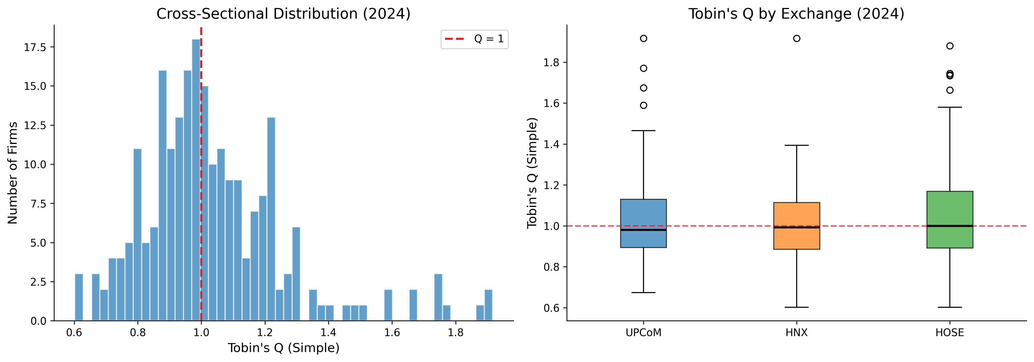
33.6 Time-Series Evolution of Tobin’s Q
# Compute annual statistics by exchange
annual_q = (
    df_clean
    .groupby(["year", "exchange"])["tobin_q_simple_w"]
    .agg(["median", lambda x: x.quantile(0.25), lambda x: x.quantile(0.75)])
    .reset_index()
)
annual_q.columns = ["year", "exchange", "median", "q25", "q75"]

fig, ax = plt.subplots(figsize=(12, 6))

exchange_colors = {"HOSE": colors["primary"], "HNX": colors["secondary"],
                   "UPCoM": colors["tertiary"]}

for exchange, color in exchange_colors.items():
    data = annual_q[annual_q["exchange"] == exchange]
    ax.plot(data["year"], data["median"], color=color, linewidth=2.5,
            label=exchange, marker="o", markersize=4)
    ax.fill_between(data["year"], data["q25"], data["q75"],
                    color=color, alpha=0.15)

ax.axhline(y=1, color="gray", linestyle="--", linewidth=1, alpha=0.7, label="Q = 1")
ax.set_xlabel("Year")
ax.set_ylabel("Tobin's Q (Median)")
ax.set_title("Evolution of Tobin's Q in the Vietnamese Market")
ax.legend(loc="upper right")
ax.set_xlim(2008, latest_year)
ax.xaxis.set_major_locator(mticker.MultipleLocator(2))

plt.tight_layout()
plt.show()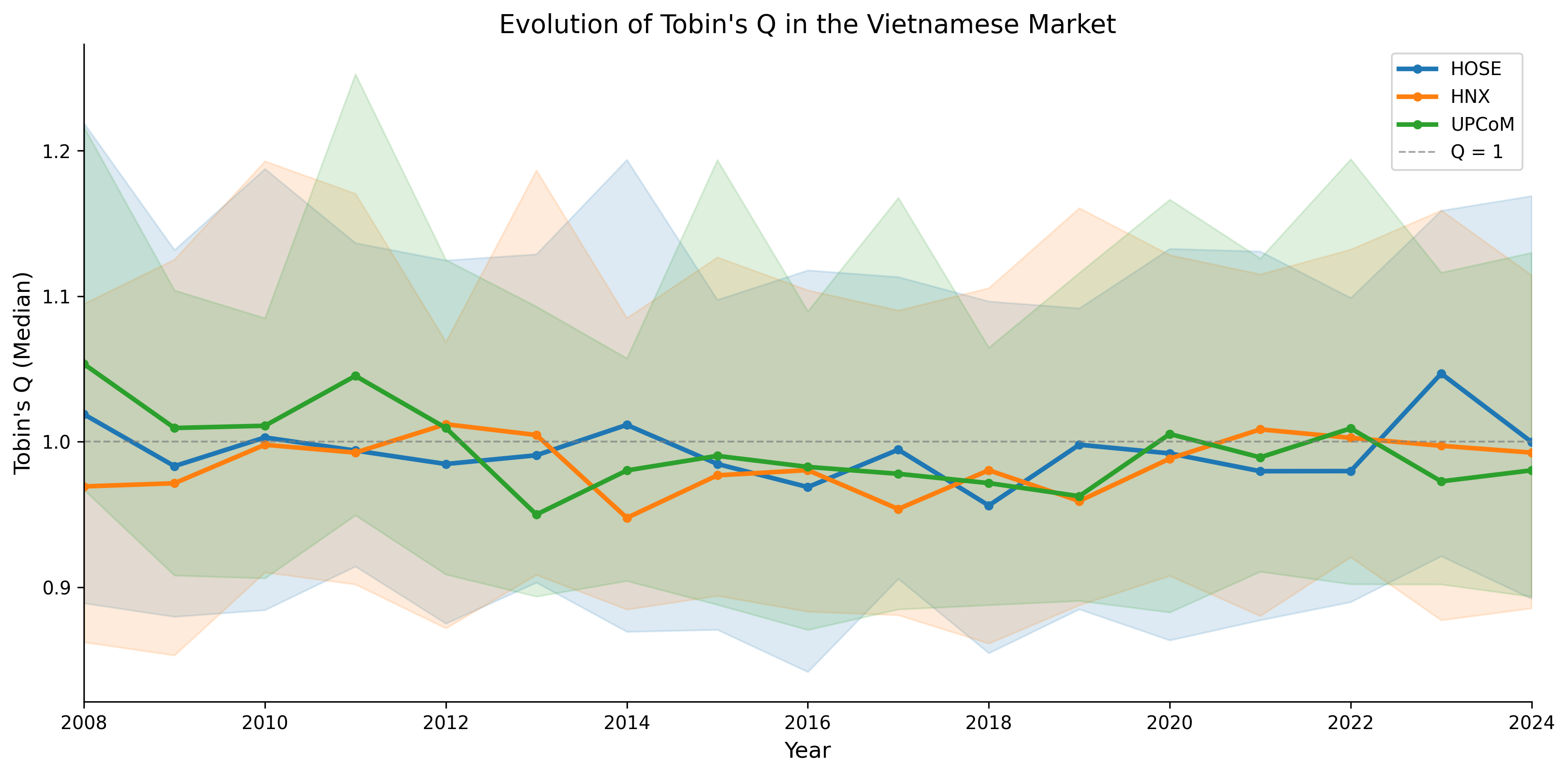
33.7 Tobin’s Q by Industry
latest_industry_q = (
    latest_data
    .groupby("industry")["tobin_q_simple_w"]
    .agg(["median", "mean", "count"])
    .reset_index()
    .sort_values("median", ascending=True)
)

fig, ax = plt.subplots(figsize=(10, 8))

bar_colors = [colors["quaternary"] if m < 1 else colors["primary"]
              for m in latest_industry_q["median"]]

ax.barh(
    latest_industry_q["industry"],
    latest_industry_q["median"],
    color=bar_colors, alpha=0.8, edgecolor="white"
)
ax.axvline(x=1, color="gray", linestyle="--", linewidth=1.5, alpha=0.7)
ax.set_xlabel("Median Tobin's Q")
ax.set_title(f"Tobin's Q by Industry ({latest_year})")

# Add count annotations
for i, (_, row) in enumerate(latest_industry_q.iterrows()):
    ax.text(row["median"] + 0.02, i, f'n={int(row["count"])}',
            va="center", fontsize=9, color="gray")

plt.tight_layout()
plt.show()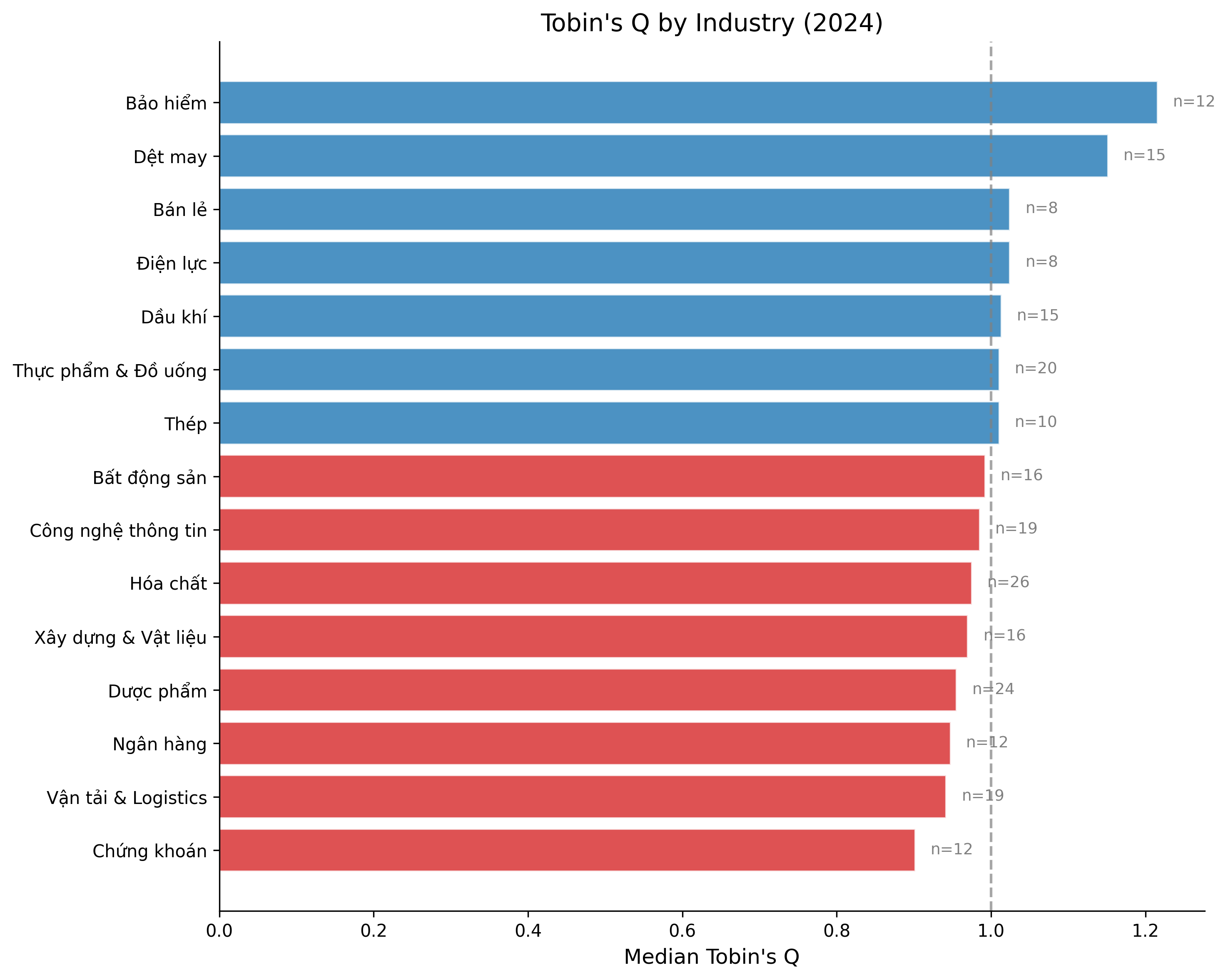
34 Computing the Altman Z-Score
34.1 Original Z-Score for Listed Firms
def compute_altman_z(df):
    """
    Compute three variants of the Altman Z-Score:
    1. Original Z-Score (for listed manufacturing firms)
    2. Z'-Score (for private firms, using book equity)
    3. Z''-Score (for emerging markets / non-manufacturing)
    """
    result = df.copy()

    # Common components
    result["wc"] = result["act"].fillna(0) - result["lct"].fillna(0)  # Working Capital

    # --- Original Z-Score ---
    # Z = 3.3*(EBIT/TA) + 0.999*(Sales/TA) + 0.6*(ME/TL) + 1.2*(WC/TA) + 1.4*(RE/TA)
    x1 = result["ebit"] / result["at"]
    x2 = result["sale"] / result["at"]
    x3 = np.where(result["tlb"] > 0, result["me"] / result["tlb"], np.nan)
    x4 = result["wc"] / result["at"]
    x5 = result["re_var"].fillna(0) / result["at"]

    result["z_x1"] = x1  # Earning power
    result["z_x2"] = x2  # Asset turnover
    result["z_x3"] = x3  # Leverage (inverse)
    result["z_x4"] = x4  # Liquidity
    result["z_x5"] = x5  # Cumulative profitability

    result["altman_z"] = (3.3 * x1 + 0.999 * x2 + 0.6 * x3 + 1.2 * x4 + 1.4 * x5)

    # --- Z'-Score (Private firms) ---
    x3_prime = np.where(result["tlb"] > 0, result["be"] / result["tlb"], np.nan)
    result["altman_z_prime"] = (
        0.717 * x4 + 0.847 * x5 + 3.107 * x1 + 0.420 * x3_prime + 0.998 * x2
    )

    # --- Z''-Score (Emerging Markets) ---
    result["altman_z_em"] = (
        3.25
        + 6.56 * x4   # Working Capital / TA
        + 3.26 * x5   # Retained Earnings / TA
        + 6.72 * x1   # EBIT / TA
        + 1.05 * x3_prime  # Book Equity / TL
    )

    # Classify risk zones
    result["z_zone"] = pd.cut(
        result["altman_z"],
        bins=[-np.inf, 1.80, 2.70, 2.99, np.inf],
        labels=["High Distress", "Distress", "Grey Zone", "Safe"]
    )

    result["z_em_zone"] = pd.cut(
        result["altman_z_em"],
        bins=[-np.inf, 1.10, 2.60, np.inf],
        labels=["Distress", "Grey Zone", "Safe"]
    )

    return result

df_clean = compute_altman_z(df_clean)

# Winsorize Z-scores
for var in ["altman_z", "altman_z_prime", "altman_z_em"]:
    df_clean[f"{var}_w"] = winsorize(df_clean[var])

print("Z-Score Summary Statistics")
z_summary = df_clean[["altman_z", "altman_z_prime", "altman_z_em"]].describe().round(3)
z_summary.columns = ["Original Z", "Z' (Private)", "Z'' (Emerging)"]
print(z_summary.to_string())
Z-Score Summary Statistics
Original Z Z' (Private) Z'' (Emerging)
count 3484.000 3484.000 3484.000
mean 2.610 2.042 7.467
std 1.896 1.194 3.137
min 0.059 0.155 1.578
25% 1.595 1.314 5.670
50% 2.212 1.806 6.987
75% 3.028 2.410 8.549
max 28.640 11.119 29.68634.2 Z-Score Component Analysis
Understanding which components drive the Z-Score is particularly informative in the Vietnamese context, where certain ratios may behave differently than in developed markets.
fig, axes = plt.subplots(2, 3, figsize=(15, 9))

components = [
    ("z_x1", 3.3, "$3.3 \\times$ EBIT/TA\n(Earning Power)"),
    ("z_x2", 0.999, "$0.999 \\times$ Sales/TA\n(Asset Turnover)"),
    ("z_x3", 0.6, "$0.6 \\times$ ME/TL\n(Leverage)"),
    ("z_x4", 1.2, "$1.2 \\times$ WC/TA\n(Liquidity)"),
    ("z_x5", 1.4, "$1.4 \\times$ RE/TA\n(Cum. Profitability)"),
]

latest_z = df_clean[df_clean["year"] == latest_year]

for idx, (var, weight, label) in enumerate(components):
    ax = axes[idx // 3, idx % 3]
    weighted_vals = (latest_z[var] * weight).dropna()
    weighted_vals = weighted_vals[weighted_vals.between(
        weighted_vals.quantile(0.01), weighted_vals.quantile(0.99)
    )]
    ax.hist(weighted_vals, bins=40, color=colors["primary"], alpha=0.7, edgecolor="white")
    ax.axvline(x=weighted_vals.median(), color=colors["quaternary"],
               linestyle="--", linewidth=2, label=f"Median: {weighted_vals.median():.2f}")
    ax.set_title(label, fontsize=11)
    ax.legend(fontsize=9)

# Remove empty subplot
axes[1, 2].set_visible(False)

plt.suptitle(f"Z-Score Component Distributions ({latest_year})", fontsize=14, y=1.02)
plt.tight_layout()
plt.show()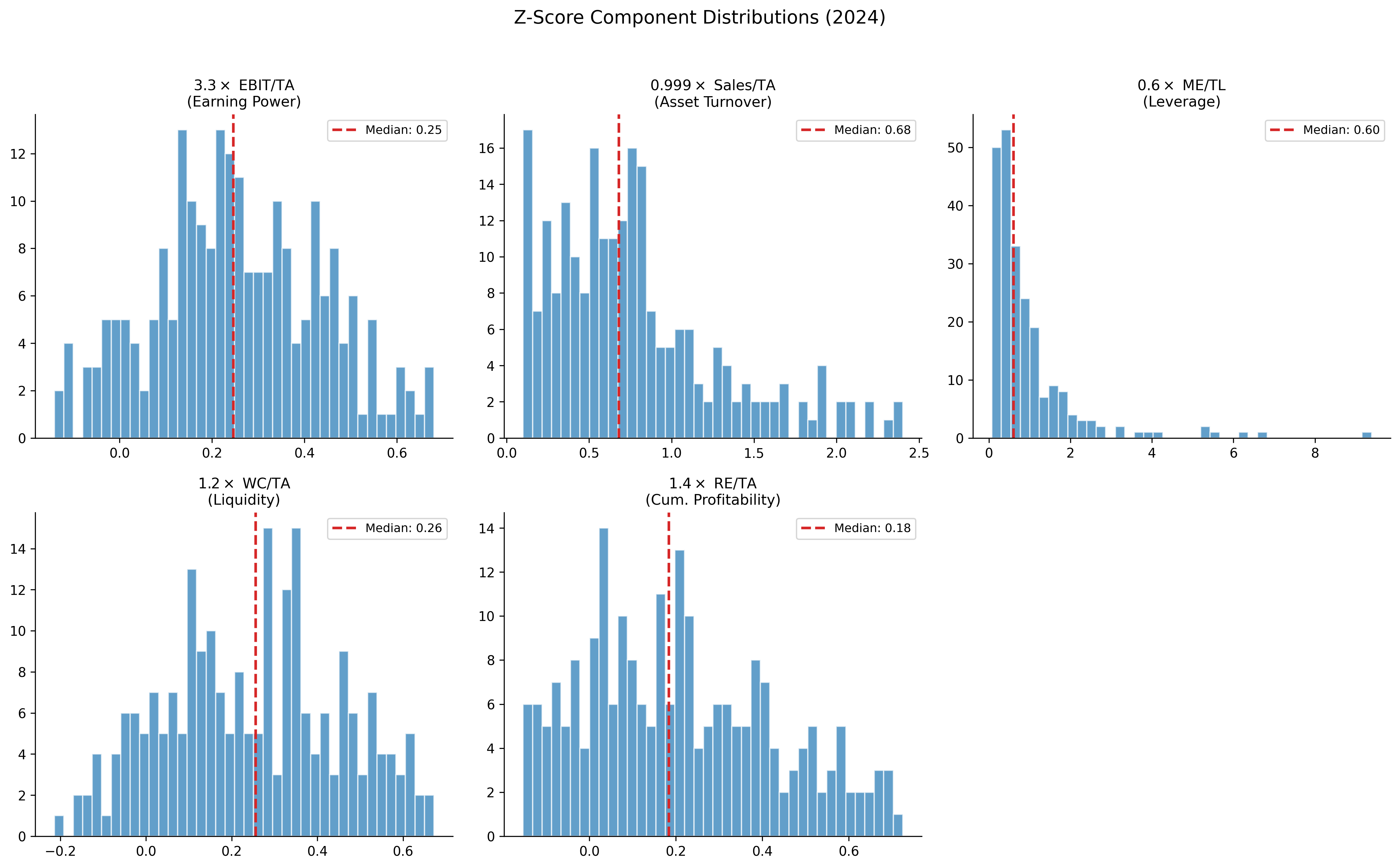
34.3 Distribution of Risk Zones
fig, axes = plt.subplots(1, 2, figsize=(14, 6))

# --- Original Z-Score Zones ---
zone_counts = (
    df_clean
    .groupby(["year", "z_zone"])
    .size()
    .unstack(fill_value=0)
)
zone_pcts = zone_counts.div(zone_counts.sum(axis=1), axis=0) * 100

zone_colors = {
    "Safe": colors["safe"],
    "Grey Zone": colors["alert"],
    "Distress": colors["quaternary"],
    "High Distress": colors["distress"],
}

axes[0].stackplot(
    zone_pcts.index,
    *[zone_pcts[col] for col in ["Safe", "Grey Zone", "Distress", "High Distress"]
      if col in zone_pcts.columns],
    labels=[col for col in ["Safe", "Grey Zone", "Distress", "High Distress"]
            if col in zone_pcts.columns],
    colors=[zone_colors[col] for col in ["Safe", "Grey Zone", "Distress", "High Distress"]
            if col in zone_pcts.columns],
    alpha=0.8
)
axes[0].set_xlabel("Year")
axes[0].set_ylabel("Percentage of Firms")
axes[0].set_title("Original Z-Score Risk Zones")
axes[0].legend(loc="upper right", fontsize=9)
axes[0].set_ylim(0, 100)

# --- Emerging Market Z''-Score Zones ---
em_zone_counts = (
    df_clean
    .groupby(["year", "z_em_zone"])
    .size()
    .unstack(fill_value=0)
)
em_zone_pcts = em_zone_counts.div(em_zone_counts.sum(axis=1), axis=0) * 100

em_zone_colors = {"Safe": colors["safe"], "Grey Zone": colors["alert"],
                  "Distress": colors["quaternary"]}

axes[1].stackplot(
    em_zone_pcts.index,
    *[em_zone_pcts[col] for col in ["Safe", "Grey Zone", "Distress"]
      if col in em_zone_pcts.columns],
    labels=[col for col in ["Safe", "Grey Zone", "Distress"]
            if col in em_zone_pcts.columns],
    colors=[em_zone_colors[col] for col in ["Safe", "Grey Zone", "Distress"]
            if col in em_zone_pcts.columns],
    alpha=0.8
)
axes[1].set_xlabel("Year")
axes[1].set_ylabel("Percentage of Firms")
axes[1].set_title("Emerging Market Z''-Score Risk Zones")
axes[1].legend(loc="upper right", fontsize=9)
axes[1].set_ylim(0, 100)

plt.tight_layout()
plt.show()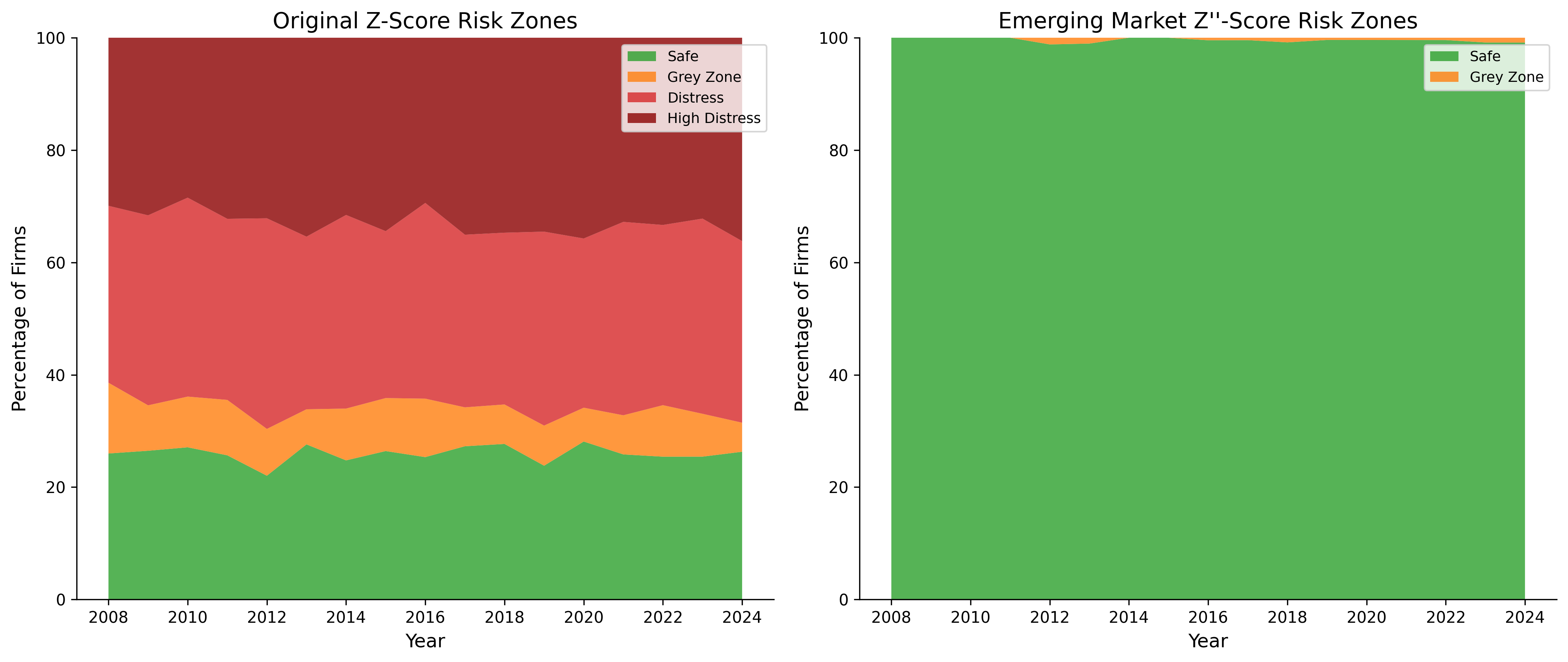
34.4 Comparing Z-Score Variants
An important practical question is which Z-Score variant is most appropriate for Vietnamese firms. The original model was calibrated on U.S. manufacturing firms, while the Z’’-Score was specifically designed for emerging markets and non-manufacturing sectors.
fig, ax = plt.subplots(figsize=(8, 8))

sample = latest_z.dropna(subset=["altman_z_w", "altman_z_em_w"]).sample(
    min(500, len(latest_z)), random_state=42
)

scatter = ax.scatter(
    sample["altman_z_w"], sample["altman_z_em_w"],
    c=sample["tobin_q_simple_w"], cmap="RdYlGn",
    alpha=0.6, s=30, edgecolor="white", linewidth=0.3
)

# Add reference lines
lims = [
    min(ax.get_xlim()[0], ax.get_ylim()[0]),
    max(ax.get_xlim()[1], ax.get_ylim()[1])
]
ax.plot(lims, lims, "k--", alpha=0.3, linewidth=1, label="45° line")

# Add zone boundaries
ax.axvline(x=1.80, color="red", linestyle=":", alpha=0.5, linewidth=1)
ax.axvline(x=2.99, color="green", linestyle=":", alpha=0.5, linewidth=1)
ax.axhline(y=1.10, color="red", linestyle=":", alpha=0.5, linewidth=1)
ax.axhline(y=2.60, color="green", linestyle=":", alpha=0.5, linewidth=1)

ax.set_xlabel("Original Z-Score")
ax.set_ylabel("Emerging Market Z''-Score")
ax.set_title("Z-Score vs Z''-Score for Vietnamese Firms")

cbar = plt.colorbar(scatter, ax=ax, shrink=0.8)
cbar.set_label("Tobin's Q")

ax.legend(loc="upper left")
plt.tight_layout()
plt.show()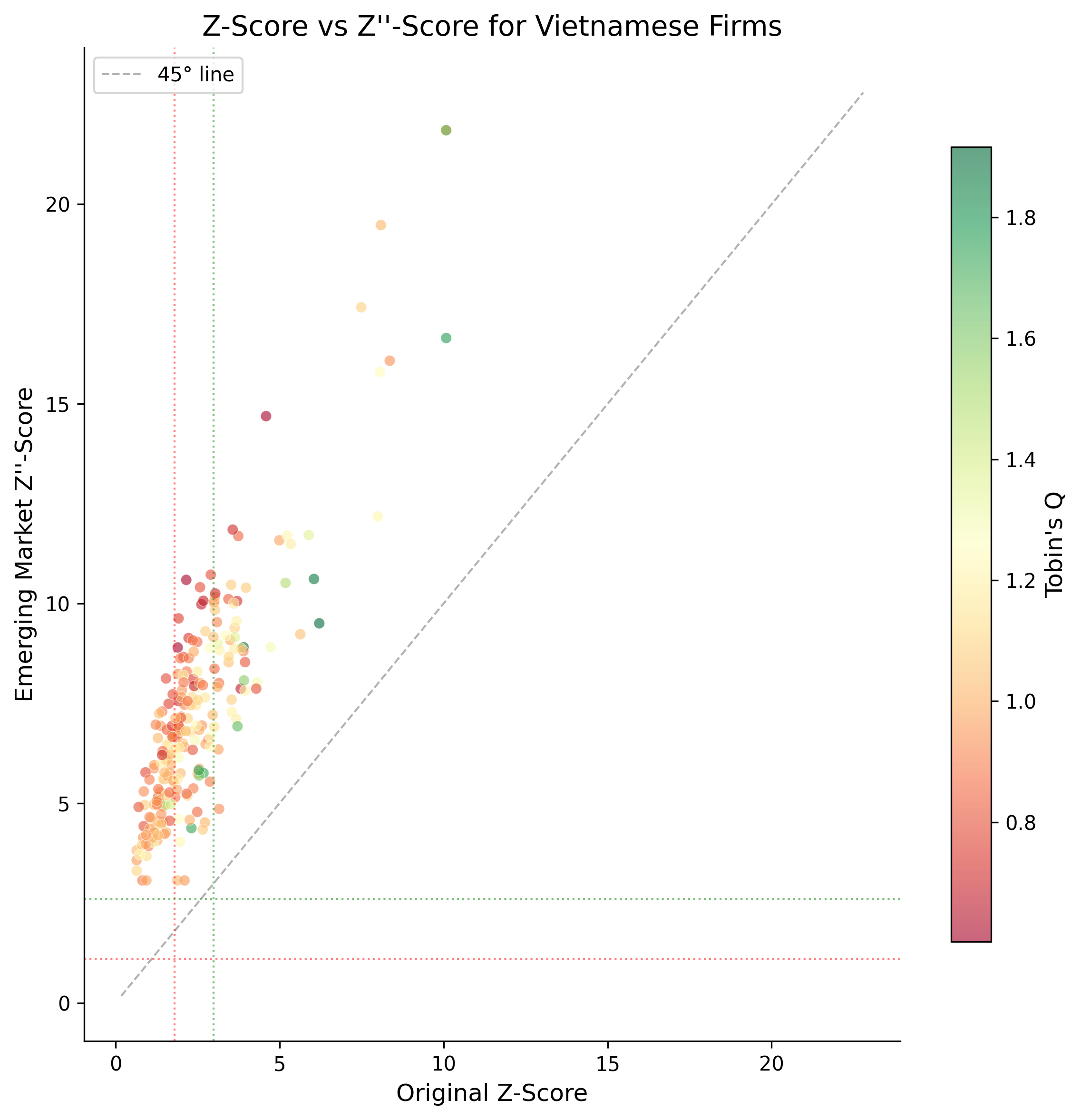
35 Computing Company Age
35.1 Multiple Age Proxies
For Vietnamese firms, we compute three age measures:
\[ \text{Age}_{\text{founding}} = \text{Current Year} - \text{Founding Year} \tag{35.1}\]
\[ \text{Age}_{\text{listing}} = \text{Current Year} - \text{Listing Year} \tag{35.2}\]
\[ \text{Age}_{\text{data}} = \text{Current Year} - \text{First Year with Data} \tag{35.3}\]
def compute_company_age(df):
    """
    Compute multiple proxies for company age.

    For Vietnamese firms:
    - Founding age: based on founding/incorporation date
    - Listing age: based on first listing on HOSE/HNX/UPCoM
    - Data age: based on first year with available financial data
    """
    result = df.copy()

    # Founding age
    result["age_founding"] = result["year"] - result["founding_year"]

    # Listing age
    result["age_listing"] = result["year"] - result["listing_year"]
    result["age_listing"] = result["age_listing"].clip(lower=0)

    # Data age (years since first available financial data)
    first_year = result.groupby("ticker")["year"].transform("min")
    result["age_data"] = result["year"] - first_year

    # Log of age (commonly used in regressions)
    result["ln_age_founding"] = np.log1p(result["age_founding"])
    result["ln_age_listing"] = np.log1p(result["age_listing"])

    return result

df_clean = compute_company_age(df_clean)

print("Company Age Summary Statistics")
age_summary = df_clean[df_clean["year"] == latest_year][
    ["age_founding", "age_listing", "age_data"]
].describe().round(1)
age_summary.columns = ["Founding Age", "Listing Age", "Data Age"]
print(age_summary.to_string())
Company Age Summary Statistics
Founding Age Listing Age Data Age
count 232.0 232.0 232.0
mean 30.1 13.9 12.3
std 11.6 5.8 3.9
min 10.0 5.0 5.0
25% 20.0 9.0 9.0
50% 30.0 13.0 13.0
75% 40.0 19.0 16.0
max 49.0 24.0 16.035.2 Age Distribution
fig, axes = plt.subplots(1, 3, figsize=(15, 5))

age_vars = [
    ("age_founding", "Founding Age (years)", colors["primary"]),
    ("age_listing", "Listing Age (years)", colors["secondary"]),
    ("age_data", "Data Age (years)", colors["tertiary"]),
]

latest = df_clean[df_clean["year"] == latest_year]

for ax, (var, label, color) in zip(axes, age_vars):
    data = latest[var].dropna()
    ax.hist(data, bins=30, color=color, alpha=0.7, edgecolor="white")
    ax.axvline(x=data.median(), color="black", linestyle="--",
               linewidth=2, label=f"Median: {data.median():.0f}")
    ax.set_xlabel(label)
    ax.set_ylabel("Number of Firms")
    ax.legend()

axes[0].set_title("Founding Age")
axes[1].set_title("Listing Age")
axes[2].set_title("Data Age")

plt.suptitle(f"Company Age Distributions ({latest_year})", fontsize=14, y=1.02)
plt.tight_layout()
plt.show()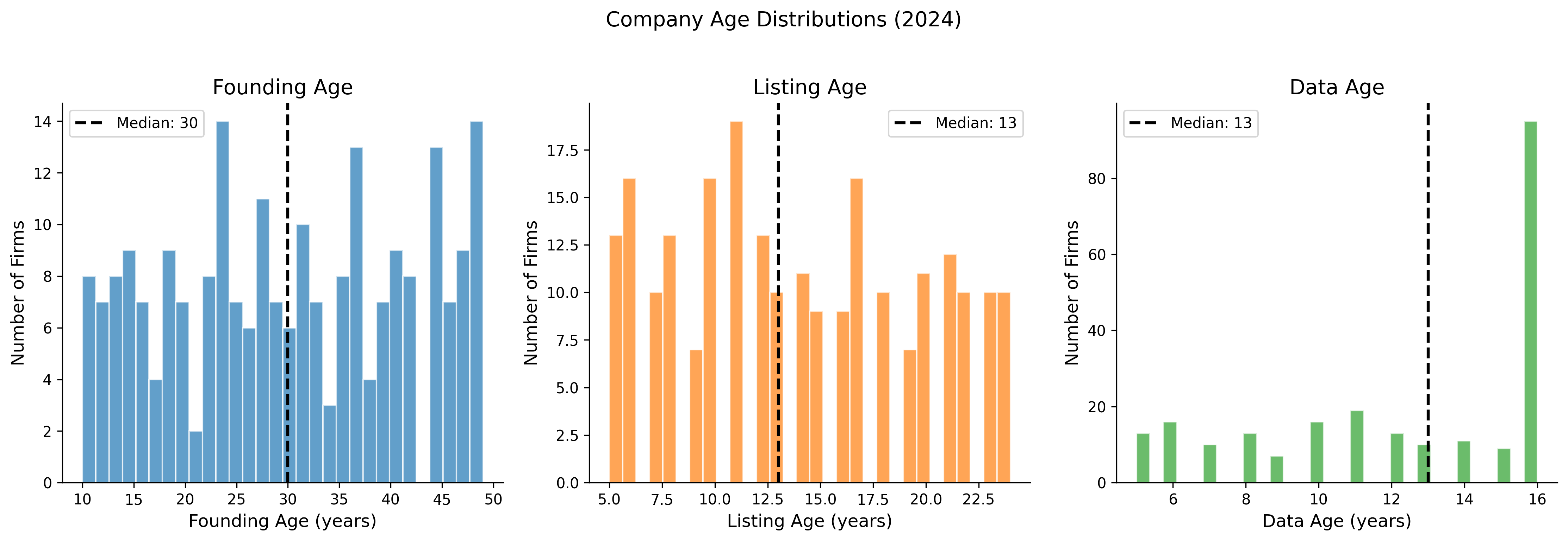
35.3 Age and the Equitization Effect
A distinctive feature of the Vietnamese market is the equitization of SOEs. Many firms have founding dates that predate the stock market by decades, creating a large gap between founding age and listing age.
fig, ax = plt.subplots(figsize=(8, 8))

latest = df_clean[df_clean["year"] == latest_year].copy()
latest["soe_flag"] = latest["state_ownership_pct"] > 30  # SOE proxy

for soe, label, color, marker in [
    (True, "SOE (>30% state)", colors["quaternary"], "s"),
    (False, "Non-SOE", colors["primary"], "o"),
]:
    subset = latest[latest["soe_flag"] == soe]
    ax.scatter(
        subset["age_listing"], subset["age_founding"],
        c=color, alpha=0.5, s=25, marker=marker, label=label, edgecolor="white"
    )

# 45-degree line
max_age = max(latest["age_founding"].max(), latest["age_listing"].max())
ax.plot([0, max_age], [0, max_age], "k--", alpha=0.3, label="Founding = Listing age")

ax.set_xlabel("Listing Age (years)")
ax.set_ylabel("Founding Age (years)")
ax.set_title("Founding vs. Listing Age: The Equitization Gap")
ax.legend()

plt.tight_layout()
plt.show()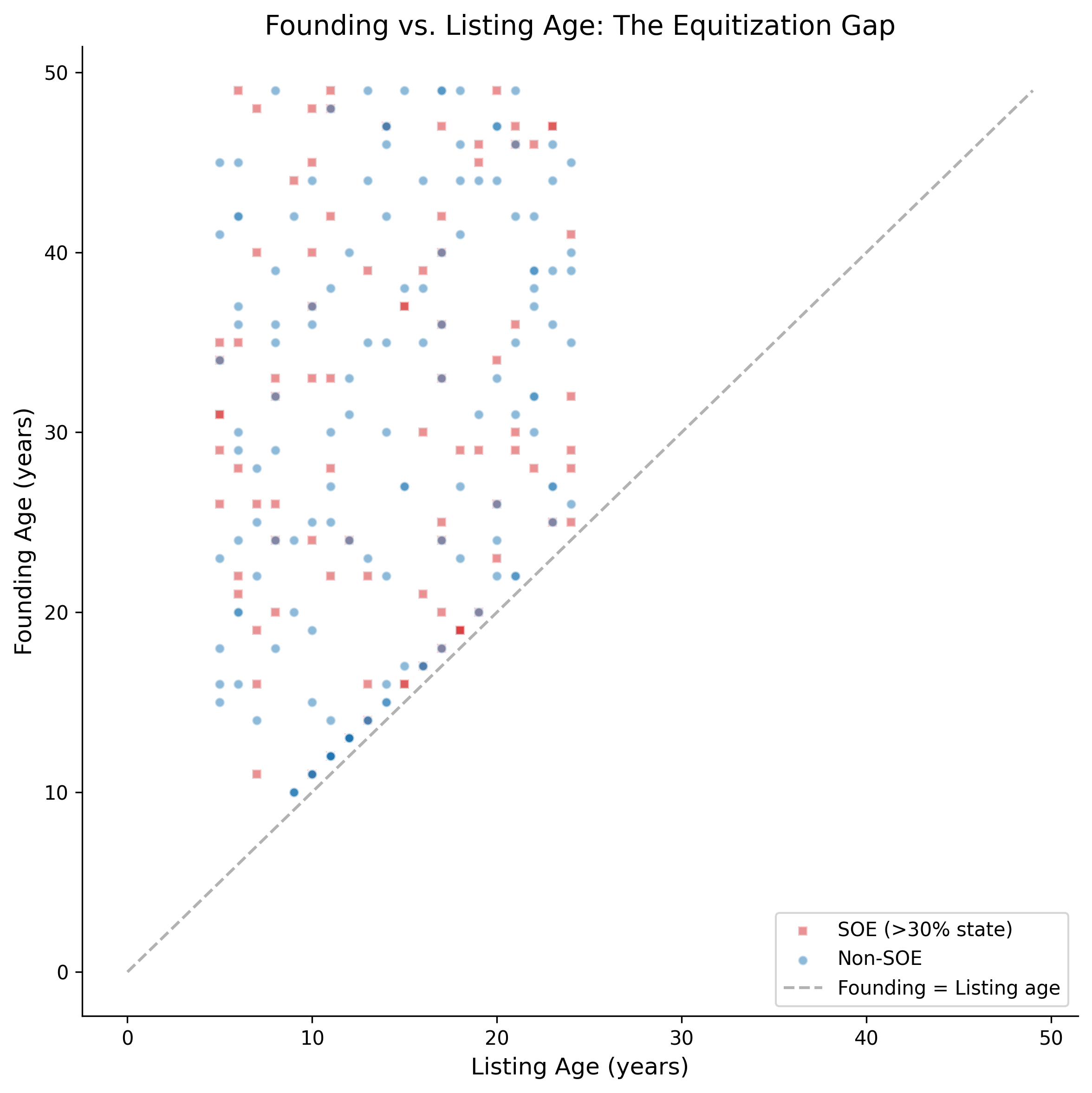
36 Joint Analysis: Valuation, Distress, and Maturity
36.1 The Relationship Between Q, Z-Score, and Age
These three measures capture different dimensions of a firm’s financial standing, but they are not independent. Theoretically, we expect:
- Q and Z: Firms with high growth opportunities (high Q) tend to be financially healthier (high Z), but the relationship is not monotonic, very high Q values may indicate speculative overvaluation.
- Q and Age: Young firms may have higher Q (growth expectations) or lower Q (unproven business model). The relationship depends on the industry life cycle.
- Z and Age: Older firms typically have more stable earnings and higher retained earnings, contributing to higher Z-Scores, though very old firms may face declining competitiveness.
fig, axes = plt.subplots(1, 3, figsize=(16, 5))

sample = latest.dropna(subset=["tobin_q_simple_w", "altman_z_w", "age_founding"])
sample = sample.sample(min(300, len(sample)), random_state=42)

# Q vs Z
axes[0].scatter(
    sample["altman_z_w"], sample["tobin_q_simple_w"],
    c=sample["age_founding"], cmap="viridis", alpha=0.6,
    s=np.log1p(sample["at"]) * 3, edgecolor="white", linewidth=0.3
)
axes[0].set_xlabel("Altman Z-Score")
axes[0].set_ylabel("Tobin's Q")
axes[0].set_title("Valuation vs. Distress Risk")
axes[0].axhline(y=1, color="gray", linestyle="--", alpha=0.5)
axes[0].axvline(x=1.80, color="red", linestyle=":", alpha=0.5)
axes[0].axvline(x=2.99, color="green", linestyle=":", alpha=0.5)

# Q vs Age
axes[1].scatter(
    sample["age_founding"], sample["tobin_q_simple_w"],
    c=sample["altman_z_w"], cmap="RdYlGn", alpha=0.6,
    s=np.log1p(sample["at"]) * 3, edgecolor="white", linewidth=0.3
)
axes[1].set_xlabel("Founding Age (years)")
axes[1].set_ylabel("Tobin's Q")
axes[1].set_title("Valuation vs. Maturity")
axes[1].axhline(y=1, color="gray", linestyle="--", alpha=0.5)

# Z vs Age
scatter = axes[2].scatter(
    sample["age_founding"], sample["altman_z_w"],
    c=sample["tobin_q_simple_w"], cmap="coolwarm", alpha=0.6,
    s=np.log1p(sample["at"]) * 3, edgecolor="white", linewidth=0.3
)
axes[2].set_xlabel("Founding Age (years)")
axes[2].set_ylabel("Altman Z-Score")
axes[2].set_title("Distress Risk vs. Maturity")
axes[2].axhline(y=1.80, color="red", linestyle=":", alpha=0.5)
axes[2].axhline(y=2.99, color="green", linestyle=":", alpha=0.5)

plt.tight_layout()
plt.show()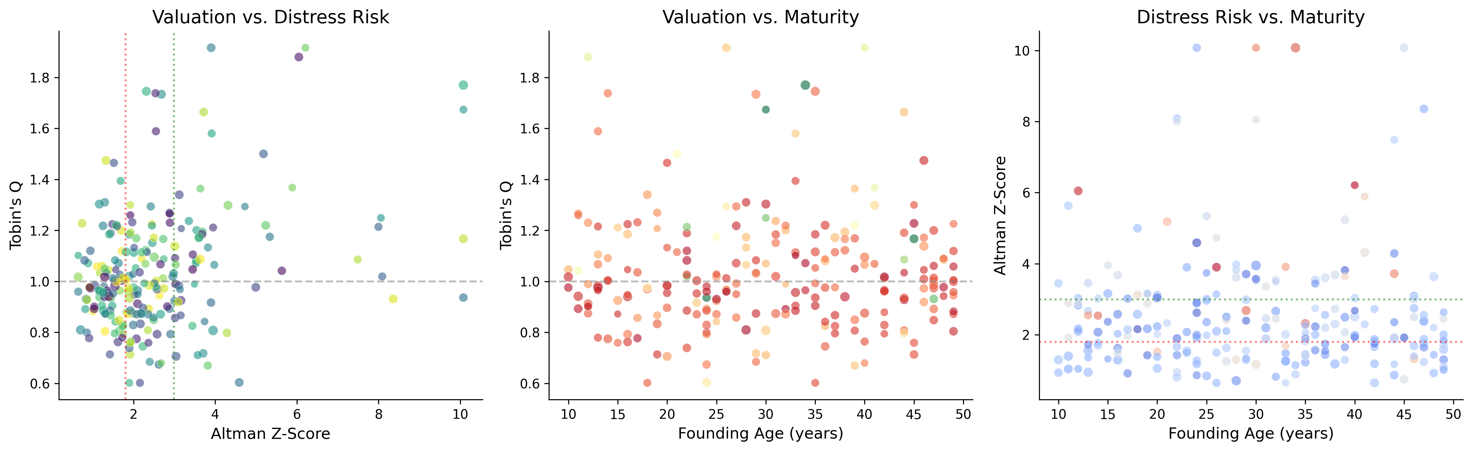
36.2 Correlation Structure
corr_vars = [
    "tobin_q_simple_w", "mtb_w", "altman_z_w", "altman_z_em_w",
    "age_founding", "age_listing",
    "z_x1", "z_x2", "z_x3", "z_x4", "z_x5"
]
corr_labels = [
    "Tobin's Q", "M/B Ratio", "Z-Score", "Z'' (EM)",
    "Age (Found.)", "Age (List.)",
    "EBIT/TA", "Sales/TA", "ME/TL", "WC/TA", "RE/TA"
]

corr_matrix = df_clean[corr_vars].corr()
corr_matrix.index = corr_labels
corr_matrix.columns = corr_labels

fig, ax = plt.subplots(figsize=(12, 10))

mask = np.triu(np.ones_like(corr_matrix, dtype=bool), k=1)
cmap = sns.diverging_palette(250, 15, s=75, l=40, n=9, center="light", as_cmap=True)

sns.heatmap(
    corr_matrix, mask=mask, cmap=cmap, center=0,
    annot=True, fmt=".2f", square=True,
    linewidths=0.5, cbar_kws={"shrink": 0.8},
    ax=ax, vmin=-1, vmax=1,
    annot_kws={"size": 9}
)
ax.set_title("Correlation Matrix of Key Financial Measures", fontsize=14, pad=20)

plt.tight_layout()
plt.show()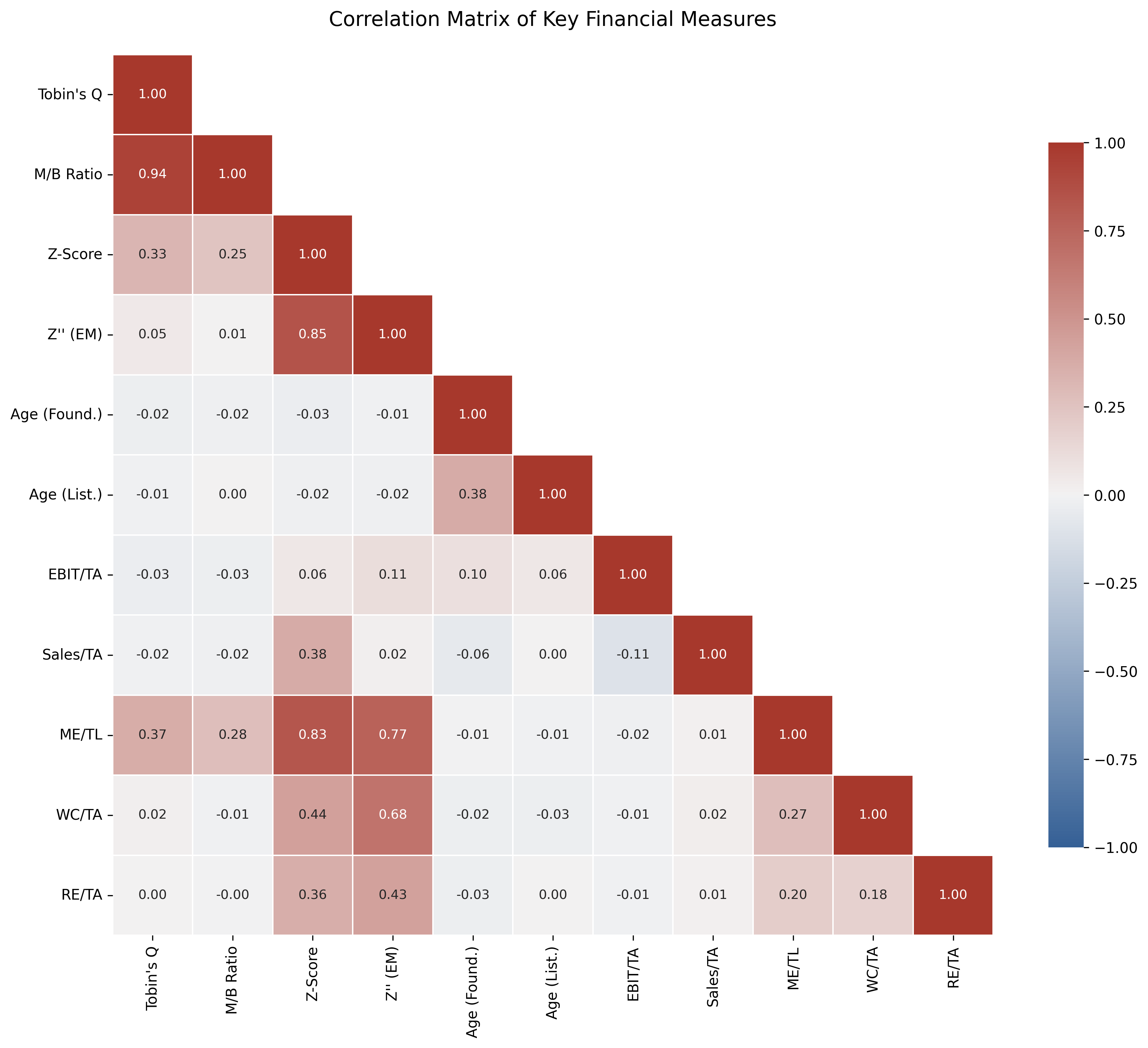
36.3 Cross-Sectional Regression Analysis
We estimate a simple cross-sectional model to examine the determinants of Tobin’s Q in the Vietnamese market:
\[ Q_{i,t} = \alpha + \beta_1 \ln(\text{Age}_{i}) + \beta_2 Z''_{i,t} + \beta_3 \text{SOE}_{i} + \beta_4 \ln(\text{TA}_{i,t}) + \varepsilon_{i,t} \tag{36.1}\]
from numpy.linalg import lstsq

# Prepare regression data
reg_data = latest.dropna(
    subset=["tobin_q_simple_w", "ln_age_founding", "altman_z_em_w", "at"]
).copy()

reg_data["ln_at"] = np.log(reg_data["at"])
reg_data["soe_dummy"] = (reg_data["state_ownership_pct"] > 30).astype(int)
reg_data["constant"] = 1.0

# OLS estimation
y = reg_data["tobin_q_simple_w"].values
X = reg_data[["constant", "ln_age_founding", "altman_z_em_w",
              "soe_dummy", "ln_at"]].values

betas, residuals, rank, sv = lstsq(X, y, rcond=None)
y_hat = X @ betas
resid = y - y_hat
n, k = X.shape

# Standard errors (heteroskedasticity-robust would be better)
sigma2 = np.sum(resid**2) / (n - k)
var_beta = sigma2 * np.linalg.inv(X.T @ X)
se = np.sqrt(np.diag(var_beta))
t_stats = betas / se
r_squared = 1 - np.sum(resid**2) / np.sum((y - y.mean())**2)
adj_r2 = 1 - (1 - r_squared) * (n - 1) / (n - k - 1)

# Display results
var_names = ["Constant", "ln(Age)", "Z''-Score (EM)", "SOE Dummy", "ln(Total Assets)"]
print("=" * 65)
print("  Cross-Sectional Regression: Determinants of Tobin's Q")
print(f"  Dependent Variable: Tobin's Q (Simple, Winsorized)")
print(f"  Sample: {n} firms ({latest_year})")
print("=" * 65)
print(f"  {'Variable':<22} {'Coef':>10} {'Std.Err':>10} {'t-stat':>10}")
print("-" * 65)
for name, b, s, t in zip(var_names, betas, se, t_stats):
    sig = "***" if abs(t) > 2.576 else "**" if abs(t) > 1.96 else "*" if abs(t) > 1.645 else ""
    print(f"  {name:<22} {b:>10.4f} {s:>10.4f} {t:>8.2f} {sig}")
print("-" * 65)
print(f"  R-squared: {r_squared:.4f}")
print(f"  Adjusted R-squared: {adj_r2:.4f}")
print(f"  Observations: {n}")
print("=" * 65)
print("  Significance: *** p<0.01, ** p<0.05, * p<0.10")
=================================================================
Cross-Sectional Regression: Determinants of Tobin's Q
Dependent Variable: Tobin's Q (Simple, Winsorized)
Sample: 232 firms (2024)
=================================================================
Variable Coef Std.Err t-stat
-----------------------------------------------------------------
Constant 0.9686 0.1959 4.94 ***
ln(Age) -0.0064 0.0365 -0.18
Z''-Score (EM) 0.0067 0.0050 1.34
SOE Dummy 0.0327 0.0315 1.04
ln(Total Assets) 0.0018 0.0096 0.19
-----------------------------------------------------------------
R-squared: 0.0126
Adjusted R-squared: -0.0092
Observations: 232
=================================================================
Significance: *** p<0.01, ** p<0.05, * p<0.1037 The Complete Pipeline
37.1 Putting It All Together
Here we provide a single, clean function that takes raw DataCore.vn financial data and produces a complete dataset with all three measures computed.
def compute_valuation_distress_age(df, firm_profiles=None):
    """
    Complete pipeline to compute Tobin's Q, Altman Z-Score variants,
    and Company Age for Vietnamese listed firms.

    Parameters
    ----------
    df : pd.DataFrame
        Panel of firm-year financial data with columns:
        at, seq, lt, lct, tlb, sale, ebit, ni, re_var, act,
        ppent, invt, txdb, itcb, pstk, me, prcc, csho, year, ticker
    firm_profiles : pd.DataFrame, optional
        Company profiles with founding_year, listing_year

    Returns
    -------
    pd.DataFrame
        Input data augmented with computed measures
    """
    result = df.copy()

    # === Data Quality Filters ===
    result = result[result["at"] > 0]
    result = result[result["seq"] > 0]

    # === Book Value of Equity (Daniel & Titman 1997) ===
    result["pref"] = result["pstk"].fillna(0)
    result["be"] = (
        result["seq"]
        + result["txdb"].fillna(0)
        + result["itcb"].fillna(0)
        - result["pref"]
    )

    # === Market Value of Equity ===
    if "me" not in result.columns or result["me"].isna().all():
        result["me"] = result["prcc"] * result["csho"]

    # === Tobin's Q Variants ===
    # Simple Q (Gompers et al. 2003)
    result["tobin_q"] = (result["at"] + result["me"] - result["be"]) / result["at"]

    # Chung-Pruitt Q
    debt_cp = (
        result["lct"].fillna(0) - result["act"].fillna(0)
        + result["invt"].fillna(0) + result["lt"].fillna(0)
    )
    result["tobin_q_cp"] = (
        (result["me"] + result["pstk"].fillna(0) + debt_cp) / result["at"]
    )

    # Market-to-Book
    result["mtb"] = np.where(result["be"] > 0, result["me"] / result["be"], np.nan)

    # === Altman Z-Score Variants ===
    result["wc"] = result["act"].fillna(0) - result["lct"].fillna(0)

    x1 = result["ebit"] / result["at"]
    x2 = result["sale"] / result["at"]
    x3_market = np.where(result["tlb"] > 0, result["me"] / result["tlb"], np.nan)
    x3_book = np.where(result["tlb"] > 0, result["be"] / result["tlb"], np.nan)
    x4 = result["wc"] / result["at"]
    x5 = result["re_var"].fillna(0) / result["at"]

    # Original Z
    result["altman_z"] = 3.3 * x1 + 0.999 * x2 + 0.6 * x3_market + 1.2 * x4 + 1.4 * x5

    # Z' (private firms)
    result["altman_z_prime"] = (
        0.717 * x4 + 0.847 * x5 + 3.107 * x1 + 0.420 * x3_book + 0.998 * x2
    )

    # Z'' (emerging markets)
    result["altman_z_em"] = (
        3.25 + 6.56 * x4 + 3.26 * x5 + 6.72 * x1 + 1.05 * x3_book
    )

    # Risk zones
    result["z_zone"] = pd.cut(
        result["altman_z"],
        bins=[-np.inf, 1.80, 2.70, 2.99, np.inf],
        labels=["High Distress", "Distress", "Grey Zone", "Safe"]
    )
    result["z_em_zone"] = pd.cut(
        result["altman_z_em"],
        bins=[-np.inf, 1.10, 2.60, np.inf],
        labels=["Distress", "Grey Zone", "Safe"]
    )

    # === Company Age ===
    if firm_profiles is not None:
        result = result.merge(
            firm_profiles[["ticker", "founding_year", "listing_year"]],
            on="ticker", how="left", suffixes=("", "_profile")
        )
        result["age_founding"] = result["year"] - result["founding_year"]
        result["age_listing"] = (result["year"] - result["listing_year"]).clip(lower=0)

    first_year = result.groupby("ticker")["year"].transform("min")
    result["age_data"] = result["year"] - first_year

    # === Winsorize ===
    for var in ["tobin_q", "tobin_q_cp", "mtb", "altman_z", "altman_z_prime", "altman_z_em"]:
        if var in result.columns:
            result[f"{var}_w"] = winsorize(result[var])

    return result

# Demonstrate the pipeline
final_df = compute_valuation_distress_age(df, firm_profiles)
print(f"Final dataset: {final_df.shape[0]:,} observations, {final_df.shape[1]} variables")
print(f"Firms: {final_df['ticker'].nunique()}")
print(f"\nKey variables computed:")
for var in ["tobin_q", "tobin_q_cp", "mtb", "altman_z", "altman_z_prime",
            "altman_z_em", "age_founding", "age_listing", "age_data"]:
    if var in final_df.columns:
        non_null = final_df[var].notna().sum()
        print(f"  {var}: {non_null:,} non-null values")
Final dataset: 3,484 observations, 48 variables
Firms: 297
Key variables computed:
tobin_q: 3,484 non-null values
tobin_q_cp: 3,484 non-null values
mtb: 3,484 non-null values
altman_z: 3,484 non-null values
altman_z_prime: 3,484 non-null values
altman_z_em: 3,484 non-null values
age_founding: 3,484 non-null values
age_listing: 3,484 non-null values
age_data: 3,484 non-null values37.2 Exporting Results
# Select key output variables
output_vars = [
    "ticker", "year", "datadate", "exchange", "industry",
    "at", "be", "me", "tobin_q", "tobin_q_w", "mtb", "mtb_w",
    "altman_z", "altman_z_w", "altman_z_em", "altman_z_em_w",
    "z_zone", "z_em_zone",
    "age_founding", "age_listing", "age_data",
    "state_ownership_pct"
]

export_cols = [v for v in output_vars if v in final_df.columns]
export_df = final_df[export_cols].copy()

# export_df.to_csv("vn_valuation_distress_age.csv", index=False)
# export_df.to_parquet("vn_valuation_distress_age.parquet", index=False)

print(f"Export dataset: {export_df.shape[0]:,} rows × {export_df.shape[1]} columns")
print(f"\nSample output (first 5 rows):")
display_cols = ["ticker", "year", "tobin_q", "altman_z", "altman_z_em",
                "z_zone", "age_founding"]
display_cols = [c for c in display_cols if c in export_df.columns]
print(export_df[display_cols].head().to_string(index=False))
Export dataset: 3,484 rows × 22 columns
Sample output (first 5 rows):
ticker year tobin_q altman_z altman_z_em z_zone age_founding
VN0001 2017 0.905928 3.345941 5.605169 Safe 4
VN0001 2018 1.270114 5.324082 9.228846 Safe 5
VN0001 2019 1.866493 5.478529 6.264178 Safe 6
VN0001 2020 1.016979 5.612289 10.445449 Safe 7
VN0001 2021 0.805818 4.220869 7.588273 Safe 838 Special Topics for the Vietnamese Market
38.1 State Ownership and Valuation
State ownership is a defining feature of the Vietnamese corporate landscape. We examine how state ownership affects both Tobin’s Q and financial distress risk.
fig, axes = plt.subplots(1, 2, figsize=(14, 6))

latest = final_df[final_df["year"] == latest_year].dropna(
    subset=["tobin_q_w", "altman_z_em_w", "state_ownership_pct"]
)

# Q vs State Ownership
axes[0].scatter(
    latest["state_ownership_pct"], latest["tobin_q_w"],
    alpha=0.4, s=20, color=colors["primary"], edgecolor="white"
)

# Binned means
bins = pd.cut(latest["state_ownership_pct"], bins=10)
binned = latest.groupby(bins)["tobin_q_w"].mean()
bin_centers = [(b.left + b.right) / 2 for b in binned.index]
axes[0].plot(bin_centers, binned.values, color=colors["quaternary"],
             linewidth=3, label="Binned Mean")

axes[0].set_xlabel("State Ownership (%)")
axes[0].set_ylabel("Tobin's Q")
axes[0].set_title("State Ownership and Firm Valuation")
axes[0].axhline(y=1, color="gray", linestyle="--", alpha=0.5)
axes[0].legend()

# Z''-Score by SOE quartile
latest["soe_quartile"] = pd.qcut(
    latest["state_ownership_pct"],
    q=4, labels=["Q1 (Low)", "Q2", "Q3", "Q4 (High)"],
    duplicates="drop"
)

soe_groups = latest.groupby("soe_quartile")["altman_z_em_w"]
box_data = [group.values for name, group in soe_groups]
bp = axes[1].boxplot(
    box_data,
    labels=[name for name, _ in soe_groups],
    patch_artist=True,
    medianprops=dict(color="black", linewidth=2)
)

gradient_colors = plt.cm.Blues(np.linspace(0.3, 0.8, len(bp["boxes"])))
for patch, color in zip(bp["boxes"], gradient_colors):
    patch.set_facecolor(color)

axes[1].axhline(y=2.60, color="green", linestyle=":", alpha=0.5, label="Safe threshold")
axes[1].axhline(y=1.10, color="red", linestyle=":", alpha=0.5, label="Distress threshold")
axes[1].set_xlabel("State Ownership Quartile")
axes[1].set_ylabel("Z''-Score (Emerging Market)")
axes[1].set_title("Financial Health by State Ownership")
axes[1].legend(fontsize=9)

plt.tight_layout()
plt.show()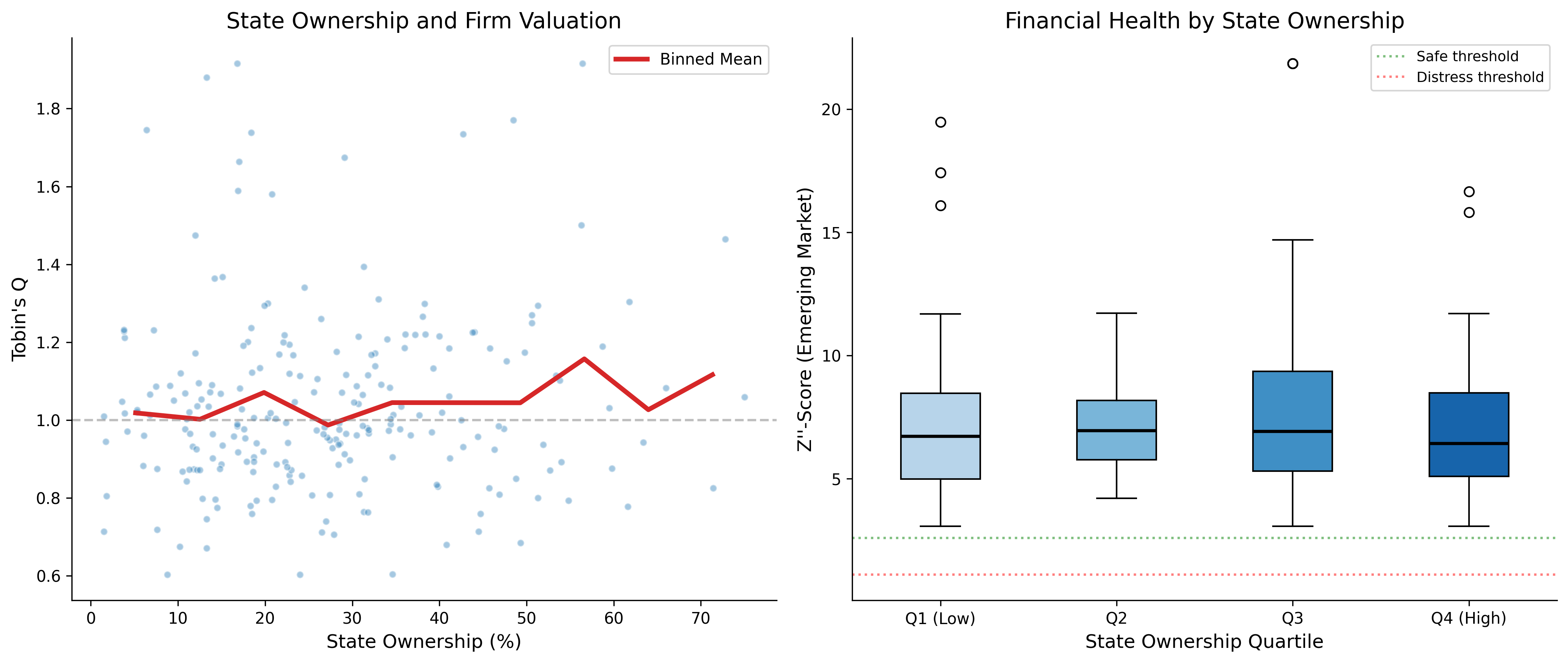
38.2 Exchange-Level Analysis
exchange_summary = (
    latest
    .groupby("exchange")
    .agg(
        n_firms=("ticker", "nunique"),
        median_q=("tobin_q_w", "median"),
        mean_q=("tobin_q_w", "mean"),
        median_z=("altman_z_w", "median"),
        mean_z_em=("altman_z_em_w", "mean"),
        pct_distress_z=("z_zone", lambda x: (x == "High Distress").mean() * 100),
        pct_distress_em=("z_em_zone", lambda x: (x == "Distress").mean() * 100),
        median_age=("age_founding", "median"),
        median_soe=("state_ownership_pct", "median"),
    )
    .round(2)
)

exchange_summary.columns = [
    "N Firms", "Median Q", "Mean Q", "Median Z", "Mean Z'' (EM)",
    "% Distress (Z)", "% Distress (Z'')", "Median Age", "Median SOE %"
]

exchange_summary.style.set_properties(**{
    "text-align": "center",
    "font-size": "10pt"
}).set_table_styles([
    {"selector": "th", "props": [
        ("background-color", "#1f77b4"),
        ("color", "white"),
        ("text-align", "center"),
        ("padding", "8px")
    ]},
]).format({
    "Median Q": "{:.2f}", "Mean Q": "{:.2f}",
    "Median Z": "{:.2f}", "Mean Z'' (EM)": "{:.2f}",
    "% Distress (Z)": "{:.1f}%", "% Distress (Z'')": "{:.1f}%",
    "Median Age": "{:.0f}", "Median SOE %": "{:.1f}%"
})| N Firms | Median Q | Mean Q | Median Z | Mean Z'' (EM) | % Distress (Z) | % Distress (Z'') | Median Age | Median SOE % | |
|---|---|---|---|---|---|---|---|---|---|
| exchange | |||||||||
| HNX | 77 | 0.99 | 1.02 | 2.07 | 7.25 | 32.5% | 0.0% | 33 | 22.1% |
| HOSE | 113 | 1.00 | 1.04 | 2.06 | 7.24 | 40.7% | 0.0% | 29 | 26.8% |
| UPCoM | 42 | 0.98 | 1.05 | 2.13 | 7.80 | 30.9% | 0.0% | 26 | 27.6% |
38.3 Sector Heatmap: Valuation and Distress
fig, axes = plt.subplots(1, 2, figsize=(16, 8))

# Tobin's Q heatmap
q_pivot = (
    final_df
    .groupby(["industry", "year"])["tobin_q_w"]
    .median()
    .unstack(fill_value=np.nan)
)

sns.heatmap(
    q_pivot, cmap="RdYlGn", center=1, ax=axes[0],
    cbar_kws={"label": "Median Q", "shrink": 0.8},
    linewidths=0.5, linecolor="white",
    xticklabels=2
)
axes[0].set_title("Tobin's Q by Industry and Year")
axes[0].set_xlabel("Year")
axes[0].set_ylabel("")

# Z''-Score heatmap
z_pivot = (
    final_df
    .groupby(["industry", "year"])["altman_z_em_w"]
    .median()
    .unstack(fill_value=np.nan)
)

sns.heatmap(
    z_pivot, cmap="RdYlGn", center=2.6, ax=axes[1],
    cbar_kws={"label": "Median Z''", "shrink": 0.8},
    linewidths=0.5, linecolor="white",
    xticklabels=2
)
axes[1].set_title("Z''-Score (EM) by Industry and Year")
axes[1].set_xlabel("Year")
axes[1].set_ylabel("")

plt.tight_layout()
plt.show()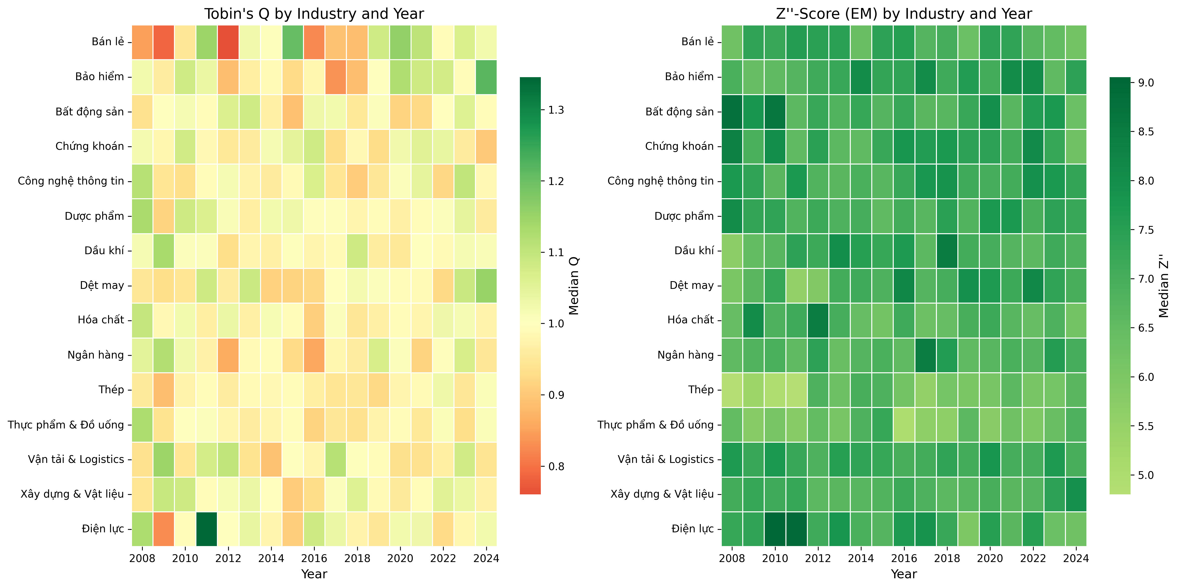
38.4 Handling Delisted Firms: Survivorship Bias
A critical issue in measuring financial distress is survivorship bias. If we only analyze currently listed firms, we miss the very firms that the Z-Score is designed to identify, those that went bankrupt or were delisted.
# Simulate delisting data (replace with DataCore.vn delisting records)
np.random.seed(123)
n_delisted = 50
delisted_firms = pd.DataFrame({
    "ticker": [f"VN{str(i).zfill(4)}" for i in range(n_firms + 1, n_firms + n_delisted + 1)],
    "delist_year": np.random.randint(2010, 2024, n_delisted),
    "delist_reason": np.random.choice(
        ["Bankruptcy/Liquidation", "Merger/Acquisition", "Voluntary Delisting",
         "Regulatory Non-compliance", "Below Minimum Requirements"],
        n_delisted,
        p=[0.15, 0.25, 0.20, 0.20, 0.20]
    )
})

# Summary of delisting reasons
print("Delisting Reasons Summary")
print("=" * 50)
reason_counts = delisted_firms["delist_reason"].value_counts()
for reason, count in reason_counts.items():
    print(f"  {reason}: {count} ({count/n_delisted*100:.0f}%)")
print(f"\nTotal delisted: {n_delisted}")
print(f"Currently listed: {final_df['ticker'].nunique()}")
print(f"\nSurvivorship rate: "
      f"{final_df['ticker'].nunique()/(final_df['ticker'].nunique()+n_delisted)*100:.1f}%")
Delisting Reasons Summary
==================================================
Merger/Acquisition: 16 (32%)
Voluntary Delisting: 14 (28%)
Regulatory Non-compliance: 9 (18%)
Below Minimum Requirements: 7 (14%)
Bankruptcy/Liquidation: 4 (8%)
Total delisted: 50
Currently listed: 297
Survivorship rate: 85.6%39 Robustness Checks and Extensions
39.1 Alternative Tobin’s Q Specifications
fig, ax = plt.subplots(figsize=(7, 7))

sample = latest.dropna(subset=["tobin_q_w", "tobin_q_cp"]).copy()
sample["tobin_q_cp_w"] = winsorize(sample["tobin_q_cp"])

ax.scatter(
    sample["tobin_q_w"], sample["tobin_q_cp_w"],
    alpha=0.4, s=15, color=colors["primary"], edgecolor="white"
)

# 45-degree line
lims = [
    min(ax.get_xlim()[0], ax.get_ylim()[0]),
    max(ax.get_xlim()[1], ax.get_ylim()[1])
]
ax.plot(lims, lims, "k--", alpha=0.3)

corr = sample["tobin_q_w"].corr(sample["tobin_q_cp_w"])
ax.text(0.05, 0.95, f"Correlation: {corr:.3f}",
        transform=ax.transAxes, fontsize=12,
        verticalalignment="top",
        bbox=dict(boxstyle="round", facecolor="wheat", alpha=0.5))

ax.set_xlabel("Simple Q (Gompers et al.)")
ax.set_ylabel("Chung-Pruitt Q")
ax.set_title("Comparison of Tobin's Q Variants")

plt.tight_layout()
plt.show()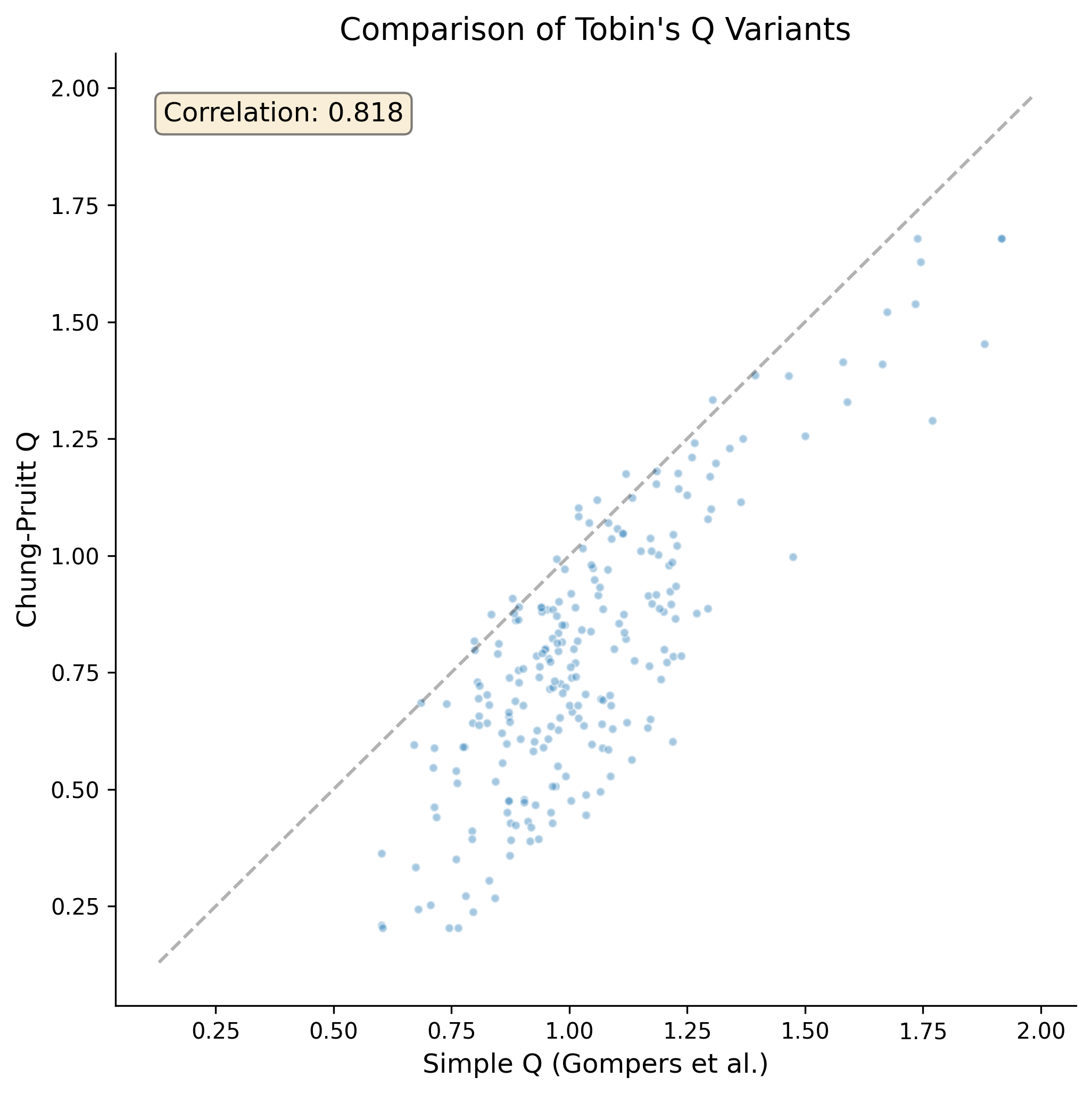
39.2 Industry-Adjusted Measures
Raw Tobin’s Q and Z-Scores may reflect industry characteristics rather than firm-specific attributes. We compute industry-adjusted versions:
\[ Q^{\text{adj}}_{i,t} = Q_{i,t} - \overline{Q}_{j(i),t} \tag{39.1}\]
where \(\overline{Q}_{j(i),t}\) is the median Tobin’s Q of the industry \(j\) to which firm \(i\) belongs in year \(t\).
def industry_adjust(df, var, group_var="industry"):
    """Compute industry-adjusted measure (deviation from industry median)."""
    industry_median = df.groupby(["year", group_var])[var].transform("median")
    return df[var] - industry_median

final_df["tobin_q_adj"] = industry_adjust(final_df, "tobin_q_w")
final_df["altman_z_em_adj"] = industry_adjust(final_df, "altman_z_em_w")

latest_adj = final_df[final_df["year"] == latest_year]

print("Industry-Adjusted Measures (Latest Year)")
print(f"  Tobin's Q (adjusted): mean={latest_adj['tobin_q_adj'].mean():.4f}, "
      f"std={latest_adj['tobin_q_adj'].std():.3f}")
print(f"  Z''-Score (adjusted): mean={latest_adj['altman_z_em_adj'].mean():.4f}, "
      f"std={latest_adj['altman_z_em_adj'].std():.3f}")
Industry-Adjusted Measures (Latest Year)
Tobin's Q (adjusted): mean=0.0352, std=0.226
Z''-Score (adjusted): mean=0.4840, std=3.03039.3 Panel Regression with Fixed Effects
For more rigorous analysis, we estimate a panel model with firm and year fixed effects:
\[ Q_{i,t} = \alpha_i + \gamma_t + \beta_1 Z''_{i,t} + \beta_2 \ln(\text{Age}_{i,t}) + \beta_3 \text{Size}_{i,t} + \varepsilon_{i,t} \tag{39.2}\]
# Simplified within-estimator (year and industry demeaning)
panel = final_df.dropna(
    subset=["tobin_q_w", "altman_z_em_w", "age_founding", "at"]
).copy()

panel["ln_at"] = np.log(panel["at"])
panel["ln_age"] = np.log1p(panel["age_founding"])

# Demean by year-industry (proxy for fixed effects)
fe_vars = ["tobin_q_w", "altman_z_em_w", "ln_age", "ln_at"]
for var in fe_vars:
    group_mean = panel.groupby(["year", "industry"])[var].transform("mean")
    panel[f"{var}_dm"] = panel[var] - group_mean

# OLS on demeaned data
y = panel["tobin_q_w_dm"].values
X = np.column_stack([
    np.ones(len(panel)),
    panel["altman_z_em_w_dm"].values,
    panel["ln_age_dm"].values,
    panel["ln_at_dm"].values,
])

betas, _, _, _ = lstsq(X, y, rcond=None)
y_hat = X @ betas
resid = y - y_hat
n, k = X.shape

sigma2 = np.sum(resid**2) / (n - k)
var_beta = sigma2 * np.linalg.inv(X.T @ X)
se = np.sqrt(np.diag(var_beta))
t_stats = betas / se
r_squared = 1 - np.sum(resid**2) / np.sum((y - y.mean())**2)

var_names = ["Constant", "Z''-Score (EM)", "ln(Age)", "ln(Total Assets)"]
print("=" * 65)
print("  Panel Regression: Tobin's Q with Year-Industry FE")
print(f"  (Within estimator via year×industry demeaning)")
print("=" * 65)
print(f"  {'Variable':<22} {'Coef':>10} {'Std.Err':>10} {'t-stat':>10}")
print("-" * 65)
for name, b, s, t in zip(var_names, betas, se, t_stats):
    sig = "***" if abs(t) > 2.576 else "**" if abs(t) > 1.96 else "*" if abs(t) > 1.645 else ""
    print(f"  {name:<22} {b:>10.4f} {s:>10.4f} {t:>8.2f} {sig}")
print("-" * 65)
print(f"  R-squared (within): {r_squared:.4f}")
print(f"  Observations: {n:,}")
print("=" * 65)
=================================================================
Panel Regression: Tobin's Q with Year-Industry FE
(Within estimator via year×industry demeaning)
=================================================================
Variable Coef Std.Err t-stat
-----------------------------------------------------------------
Constant 0.0000 0.0038 0.00
Z''-Score (EM) 0.0034 0.0014 2.45 **
ln(Age) -0.0055 0.0063 -0.88
ln(Total Assets) -0.0031 0.0026 -1.16
-----------------------------------------------------------------
R-squared (within): 0.0024
Observations: 3,484
=================================================================40 Practical Considerations and Limitations
40.1 Known Limitations of Tobin’s Q in Vietnam
Several issues affect the reliability of Tobin’s Q estimates for Vietnamese firms:
Book value as replacement cost proxy: The simplified Q measure assumes that book value of assets approximates replacement cost. Under VAS’s heavy reliance on historical cost, this assumption may be more problematic than in IFRS-adopting countries, particularly for firms with significant land use rights or long-lived tangible assets.
Market microstructure effects: Vietnam’s daily price limits can prevent market prices from reaching equilibrium, potentially distorting the market value component. Foreign ownership limits may create artificial price premiums for certain stocks.
Preferred stock rarity: While this simplifies the computation (most Vietnamese firms have no preferred stock), it means the BE calculation is dominated by common equity, which may not capture all ownership claims.
Cross-listing effects: Some Vietnamese firms are listed on multiple venues (HOSE, HNX, UPCoM, or even foreign exchanges). Care must be taken to use consistent price and share data.
40.2 Known Limitations of Altman Z-Score in Vietnam
Calibration sample: The original Z-Score was estimated on mid-20th-century U.S. manufacturing firms. The Z’’-Score for emerging markets is more appropriate but was still estimated on a non-Vietnamese sample.
Accounting differences: VAS accounting standards produce financial ratios with different distributional properties than US GAAP or IFRS data, potentially affecting the discriminant function’s classification accuracy.
Banking and financial firms: The Z-Score was not designed for financial institutions, which have fundamentally different balance sheet structures. Banks, insurance companies, and securities firms should be excluded or analyzed separately.
Implicit guarantees: SOEs and firms connected to major economic groups may have implicit support that reduces actual default risk below Z-Score predictions.
40.3 Recommendations for Researchers
Based on our analysis, we offer the following recommendations for researchers working with Vietnamese data:
- Use the Z’’-Score (Emerging Market) variant as the primary distress measure for Vietnamese non-financial firms.
- Report multiple Q variants (Simple and Chung-Pruitt) to demonstrate robustness.
- Winsorize at 1%/99% to mitigate the impact of data errors and extreme outliers.
- Compute industry-adjusted measures when making cross-sectional comparisons.
- Use founding age rather than listing age when available, but report both to distinguish organizational maturity from capital market experience.
- Exclude financial firms from Z-Score analysis.
- Account for state ownership as a moderating variable in valuation and distress studies.
41 Summary
This chapter presented a treatment of three fundamental corporate finance measures (i.e., Tobin’s Q, the Altman Z-Score, and Company Age). We covered the theoretical foundations of each measure and provided extensive visualizations of cross-sectional and time-series patterns.
Key findings from our analysis of Vietnamese listed firms include:
Tobin’s Q varies substantially across industries and exchanges, with technology and consumer-facing sectors typically commanding higher valuations. HOSE-listed firms tend to have higher Q values than HNX or UPCoM firms, reflecting both firm quality differences and liquidity effects.
The Altman Z-Score reveals that a meaningful proportion of Vietnamese firms operate in or near the distress zone, though the appropriate variant matters; the emerging market Z’’-Score provides more nuanced classification than the original model. Financial health shows significant time-series variation, with notable deterioration during economic downturns.
Company age in Vietnam requires careful treatment due to the equitization of SOEs, which creates large gaps between founding age and listing age. This distinction is substantively important for understanding the relationship between maturity, valuation, and financial stability.