import pandas as pd
import numpy as np
import tidyfinance as tf

from plotnine import *
from mizani.formatters import percent_format
from adjustText import adjust_text16 The Capital Asset Pricing Model
16.1 From Efficient Portfolios to Equilibrium Prices
The previous chapter on Modern Portfolio Theory (MPT) showed how an investor can construct portfolios that optimally trade off risk and expected return. But MPT leaves a crucial question unanswered: What determines the expected returns themselves? Why do some assets command higher risk premiums than others?
The Capital Asset Pricing Model (CAPM) answers this question. Developed simultaneously by Sharpe (1964), Lintner (1965), and Mossin (1966), the CAPM extends MPT to explain how assets should be priced in equilibrium when all investors follow mean-variance optimization principles. The CAPM’s central insight is both elegant and counterintuitive: not all risk is rewarded. Only the component of risk that cannot be diversified away (i.e., systematic risk) commands a risk premium in equilibrium.
The CAPM remains the cornerstone of asset pricing theory, not because it perfectly describes reality, but because it provides the simplest coherent framework for understanding the relationship between risk and expected return. Every extension and alternative model in asset pricing (e.g., from the Fama-French factors to consumption-based pricing) builds upon or reacts against the CAPM’s foundational logic.
In this chapter, we derive the CAPM from first principles, illustrate its theoretical underpinnings, and show how to estimate its parameters empirically. We download stock market data, estimate betas using regression analysis, and evaluate asset performance relative to model predictions.
16.2 Systematic versus Idiosyncratic Risk
Before diving into the mathematics, we need to understand the fundamental distinction that makes the CAPM work: the difference between systematic and idiosyncratic risk.
16.2.1 Idiosyncratic Risk: Diversifiable and Unrewarded
Consider events that affect individual companies but not the broader market: a CEO resigns unexpectedly, a product launch fails, earnings disappoint analysts, or a factory experiences a fire. These company-specific events can dramatically affect individual stock prices, but they tend to average out across a diversified portfolio. When one company has bad news, another often has good news; the shocks are largely uncorrelated.
This idiosyncratic (or firm-specific) risk can be eliminated through diversification. By holding a portfolio of many stocks, an investor can reduce idiosyncratic risk to nearly zero. Since this risk can be avoided at no cost, investors should not expect compensation for bearing it. In equilibrium, idiosyncratic risk earns no premium.
16.2.2 Systematic Risk: Undiversifiable and Priced
Systematic risk, by contrast, affects all assets simultaneously. Recessions, interest rate changes, geopolitical crises, and pandemics impact virtually every company to some degree. No amount of diversification can eliminate exposure to these economy-wide shocks, they are inherent to participating in the market.
Since systematic risk cannot be diversified away, investors genuinely dislike it. They must be compensated for bearing it. The CAPM formalizes this intuition: expected returns should depend only on systematic risk, not total risk. Two assets with identical total volatility can have very different expected returns if their systematic risk exposures differ.
16.2.3 A Simple Illustration
Imagine two stocks with identical 30% annual volatility. Stock A is a gold mining company whose returns move opposite to the overall market: it does well when the economy struggles and poorly when it booms. Stock B is a luxury retailer that amplifies market movements: soaring in good times and crashing in bad times.
Which stock should offer higher expected returns? Intuition might suggest they should be equal since both have the same volatility. But the CAPM says Stock B should offer substantially higher returns. Why? Because Stock B performs poorly precisely when investors’ overall wealth is already down (during market crashes), making its returns particularly painful. Stock A, by contrast, provides insurance. Its strong performance during market downturns partially offsets losses elsewhere in the portfolio. Investors value this insurance property and are willing to accept lower expected returns in exchange.
This is the CAPM’s core insight: expected returns compensate investors for systematic risk exposure, measured by how an asset’s returns co-move with the market portfolio.
16.3 Data Preparation
Building on our analysis from the previous chapter, we examine the VN30 constituents as our asset universe. We download and prepare monthly return data:
vn30_symbols = [
    "ACB", "BCM", "BID", "BVH", "CTG", "FPT", "GAS", "GVR", "HDB", "HPG",
    "MBB", "MSN", "MWG", "PLX", "POW", "SAB", "SHB", "SSB", "STB", "TCB",
    "TPB", "VCB", "VHM", "VIB", "VIC", "VJC", "VNM", "VPB", "VRE", "EIB"
]
import os
import boto3
from botocore.client import Config
from io import BytesIO
class ConnectMinio:
def __init__(self):
self.MINIO_ENDPOINT = os.environ["MINIO_ENDPOINT"]
self.MINIO_ACCESS_KEY = os.environ["MINIO_ACCESS_KEY"]
self.MINIO_SECRET_KEY = os.environ["MINIO_SECRET_KEY"]
self.REGION = os.getenv("MINIO_REGION", "us-east-1")
self.s3 = boto3.client(
"s3",
endpoint_url=self.MINIO_ENDPOINT,
aws_access_key_id=self.MINIO_ACCESS_KEY,
aws_secret_access_key=self.MINIO_SECRET_KEY,
region_name=self.REGION,
config=Config(signature_version="s3v4"),
)
def test_connection(self):
resp = self.s3.list_buckets()
print("Connected. Buckets:")
for b in resp.get("Buckets", []):
print(" -", b["Name"])
conn = ConnectMinio()
s3 = conn.s3
conn.test_connection()
bucket_name = os.environ["MINIO_BUCKET"]
prices = pd.read_csv(
BytesIO(
s3.get_object(
Bucket=bucket_name,
Key="historycal_price/dataset_historical_price.csv"
)["Body"].read()
),
low_memory=False
)Connected. Buckets:
- dsteam-data
- rawbctcWe process the raw price data to compute adjusted closing prices and standardize column names:
prices["date"] = pd.to_datetime(prices["date"])
prices["adjusted_close"] = prices["close_price"] * prices["adj_ratio"]
prices = prices.rename(columns={
    "vol_total": "volume",
    "open_price": "open",
    "low_price": "low",
    "high_price": "high",
    "close_price": "close"
})
prices = prices.sort_values(["symbol", "date"])
prices_daily = prices[prices["symbol"].isin(vn30_symbols)]
prices_daily[["date", "symbol", "adjusted_close"]].head(3)| date | symbol | adjusted_close | |
|---|---|---|---|
| 18176 | 2010-01-04 | ACB | 329.408244 |
| 18177 | 2010-01-05 | ACB | 329.408244 |
| 18178 | 2010-01-06 | ACB | 320.258015 |
16.3.1 Computing Monthly Returns
We aggregate daily prices to monthly frequency. Using monthly returns rather than daily returns offers several advantages for portfolio analysis: monthly returns exhibit less noise, better approximate normality, and reduce the impact of microstructure effects like bid-ask bounce.
returns_monthly = (prices_daily
    .assign(
        date=prices_daily["date"].dt.to_period("M").dt.to_timestamp("M")
    )
    .groupby(["symbol", "date"], as_index=False)
    .agg(adjusted_close=("adjusted_close", "last"))
    .sort_values(["symbol", "date"])
    .assign(
        ret=lambda x: x.groupby("symbol")["adjusted_close"].pct_change()
    )
)

returns_monthly.head(3)| symbol | date | adjusted_close | ret | |
|---|---|---|---|---|
| 0 | ACB | 2010-01-31 | 291.975489 | NaN |
| 1 | ACB | 2010-02-28 | 303.621235 | 0.039886 |
| 2 | ACB | 2010-03-31 | 273.784658 | -0.098269 |
16.4 The Risk-Free Asset and the Investment Opportunity Set
16.4.1 Adding a Risk-Free Asset
The previous chapter on MPT considered portfolios composed entirely of risky assets, requiring that portfolio weights sum to one. The CAPM introduces a crucial new element: a risk-free asset that pays a constant interest rate \(r_f\) with zero volatility.
This seemingly simple addition fundamentally transforms the investment opportunity set. With a risk-free asset available, investors can choose to park some wealth in the safe asset and invest the remainder in risky assets. They can also borrow at the risk-free rate to leverage their risky positions.
Let \(\omega \in \mathbb{R}^N\) denote the portfolio weights in the \(N\) risky assets. Unlike before, these weights need not sum to one. The remainder, \(1 - \iota'\omega\) (where \(\iota\) is a vector of ones), is invested in the risk-free asset.
16.4.2 Portfolio Return with a Risk-Free Asset
The expected return on this combined portfolio is:
\[ \mu_\omega = \omega'\mu + (1 - \iota'\omega)r_f = r_f + \omega'(\mu - r_f) = r_f + \omega'\tilde{\mu} \]
where \(\mu\) is the vector of expected returns on risky assets and \(\tilde{\mu} = \mu - r_f\) denotes the vector of excess returns (returns above the risk-free rate).
This expression reveals an important decomposition: the portfolio’s expected return equals the risk-free rate plus a risk premium determined by the exposure to risky assets.
16.4.3 Portfolio Variance
Since the risk-free asset has zero volatility and zero covariance with risky assets, only the risky portion contributes to portfolio variance:
\[ \sigma_\omega^2 = \omega'\Sigma\omega \]
where \(\Sigma\) is the variance-covariance matrix of risky asset returns. The portfolio’s volatility (standard deviation) is:
\[ \sigma_\omega = \sqrt{\omega'\Sigma\omega} \]
16.4.4 Setting Up the Risk-Free Rate
For a realistic proxy of the risk-free rate, we use the Vietnam government bond yield. Government bonds of stable economies are considered “risk-free” because the government can always print money to meet its obligations (though this may cause inflation).
all_dates = pd.date_range(
    start=returns_monthly["date"].min(),
    end=returns_monthly["date"].max(),
    freq="ME"
)

# Vietnam 10-Year Government Bond Yield (approximately 2.52% annualized)
rf_annual = 0.0252
rf_monthly_val = (1 + rf_annual)**(1/12) - 1

risk_free_monthly = pd.DataFrame({
    "date": all_dates,
    "risk_free": rf_monthly_val
})

risk_free_monthly["date"] = (
    pd.to_datetime(risk_free_monthly["date"])
    .dt.to_period("M")
    .dt.to_timestamp("M")
)

risk_free_monthly.head(3)| date | risk_free | |
|---|---|---|
| 0 | 2010-01-31 | 0.002076 |
| 1 | 2010-02-28 | 0.002076 |
| 2 | 2010-03-31 | 0.002076 |
We merge the risk-free rate with our returns data and compute excess returns:
returns_monthly = returns_monthly.merge(
    risk_free_monthly[["date", "risk_free"]],
    on="date",
    how="left"
)

rf = risk_free_monthly["risk_free"].mean()

returns_monthly = (returns_monthly
    .assign(
        ret_excess=lambda x: x["ret"] - x["risk_free"]
    )
    .assign(
        ret_excess=lambda x: x["ret_excess"].clip(lower=-1)
    )
)

returns_monthly.head(3)| symbol | date | adjusted_close | ret | risk_free | ret_excess | |
|---|---|---|---|---|---|---|
| 0 | ACB | 2010-01-31 | 291.975489 | NaN | 0.002076 | NaN |
| 1 | ACB | 2010-02-28 | 303.621235 | 0.039886 | 0.002076 | 0.037810 |
| 2 | ACB | 2010-03-31 | 273.784658 | -0.098269 | 0.002076 | -0.100345 |
16.5 The Tangency Portfolio: Where Everyone Invests
16.5.1 Deriving the Optimal Risky Portfolio
With a risk-free asset available, how should an investor allocate wealth across risky assets? Consider an investor who wants to achieve a target expected excess return \(\bar{\mu}\) with minimum variance. The optimization problem becomes:
\[ \min_\omega \omega'\Sigma\omega \quad \text{subject to} \quad \omega'\tilde{\mu} = \bar{\mu} \]
Using the Lagrangian method:
\[ \mathcal{L}(\omega, \lambda) = \omega'\Sigma\omega - \lambda(\omega'\tilde{\mu} - \bar{\mu}) \]
The first-order condition with respect to \(\omega\) is:
\[ \frac{\partial \mathcal{L}}{\partial \omega} = 2\Sigma\omega - \lambda\tilde{\mu} = 0 \]
Solving for the optimal weights:
\[ \omega^* = \frac{\lambda}{2}\Sigma^{-1}\tilde{\mu} \]
The constraint \(\omega'\tilde{\mu} = \bar{\mu}\) determines \(\lambda\):
\[ \bar{\mu} = \tilde{\mu}'\omega^* = \frac{\lambda}{2}\tilde{\mu}'\Sigma^{-1}\tilde{\mu} \implies \lambda = \frac{2\bar{\mu}}{\tilde{\mu}'\Sigma^{-1}\tilde{\mu}} \]
Substituting back:
\[ \omega^* = \frac{\bar{\mu}}{\tilde{\mu}'\Sigma^{-1}\tilde{\mu}}\Sigma^{-1}\tilde{\mu} \]
16.5.2 The Tangency Portfolio
Notice something remarkable: the direction of \(\omega^*\) is always \(\Sigma^{-1}\tilde{\mu}\), regardless of the target return \(\bar{\mu}\). Only the scale changes. This means all investors, regardless of their risk preferences, hold the same portfolio of risky assets. They differ only in how much they allocate to this portfolio versus the risk-free asset.
To obtain the portfolio of risky assets that is fully invested (weights summing to one), we normalize:
\[ \omega_{\text{tan}} = \frac{\omega^*}{\iota'\omega^*} = \frac{\Sigma^{-1}(\mu - r_f)}{\iota'\Sigma^{-1}(\mu - r_f)} \]
This is called the tangency portfolio (or maximum Sharpe ratio portfolio) because it lies at the point where the efficient frontier is tangent to the capital market line.
16.5.3 The Sharpe Ratio and the Capital Market Line
The Sharpe ratio measures excess return per unit of volatility:
\[ \text{Sharpe Ratio} = \frac{\mu_p - r_f}{\sigma_p} \]
The tangency portfolio maximizes the Sharpe ratio among all possible portfolios. Any combination of the risk-free asset and the tangency portfolio lies on a straight line in mean-standard deviation space, called the Capital Market Line (CML):
\[ \mu_p = r_f + \left(\frac{\mu_{\text{tan}} - r_f}{\sigma_{\text{tan}}}\right)\sigma_p \]
The slope of this line equals the Sharpe ratio of the tangency portfolio (i.e., the highest achievable Sharpe ratio).
16.5.4 Computing the Tangency Portfolio
Let’s compute the tangency portfolio for our VN30 universe:
assets = (returns_monthly
    .groupby("symbol", as_index=False)
    .agg(
        mu=("ret", "mean"),
        sigma=("ret", "std")
    )
)

sigma = (returns_monthly
    .pivot(index="date", columns="symbol", values="ret")
    .cov()
)

mu = (returns_monthly
    .groupby("symbol")["ret"]
    .mean()
    .values
)
# Compute tangency portfolio weights
w_tan = np.linalg.solve(sigma, mu - rf)
w_tan = w_tan / np.sum(w_tan)
# Portfolio performance metrics
mu_w = w_tan.T @ mu
sigma_w = np.sqrt(w_tan.T @ sigma @ w_tan)
efficient_portfolios = pd.DataFrame([
{"symbol": r"$\omega_{\mathrm{tan}}$", "mu": mu_w, "sigma": sigma_w},
{"symbol": r"$r_f$", "mu": rf, "sigma": 0}
])
sharpe_ratio = (mu_w - rf) / sigma_w
print(f"Tangency Portfolio Sharpe Ratio: {sharpe_ratio:.4f}")
print(efficient_portfolios)Tangency Portfolio Sharpe Ratio: -0.5552
symbol mu sigma
0 $\omega_{\mathrm{tan}}$ -0.041157 0.077866
1 $r_f$ 0.002076 0.00000016.5.5 Visualizing the Efficient Frontier with a Risk-Free Asset
Figure 16.1 shows the efficient frontier when a risk-free asset is available. The frontier is now a straight line (the Capital Market Line) connecting the risk-free asset to the tangency portfolio and extending beyond.
efficient_portfolios_figure = (
    ggplot(efficient_portfolios, aes(x="sigma", y="mu"))
    + geom_point(data=assets)
    + geom_point(data=efficient_portfolios, color="blue", size=3)
    + geom_label(
        aes(label="symbol"),
        adjust_text={"arrowprops": {"arrowstyle": "-"}}
    )
    + scale_x_continuous(labels=percent_format())
    + scale_y_continuous(labels=percent_format())
    + labs(
        x="Volatility (Standard Deviation)",
        y="Expected Return",
        title="Efficient Frontier with Risk-Free Asset (VN30)"
    )
    + geom_abline(slope=sharpe_ratio, intercept=rf, linetype="dotted")
)

efficient_portfolios_figure.show()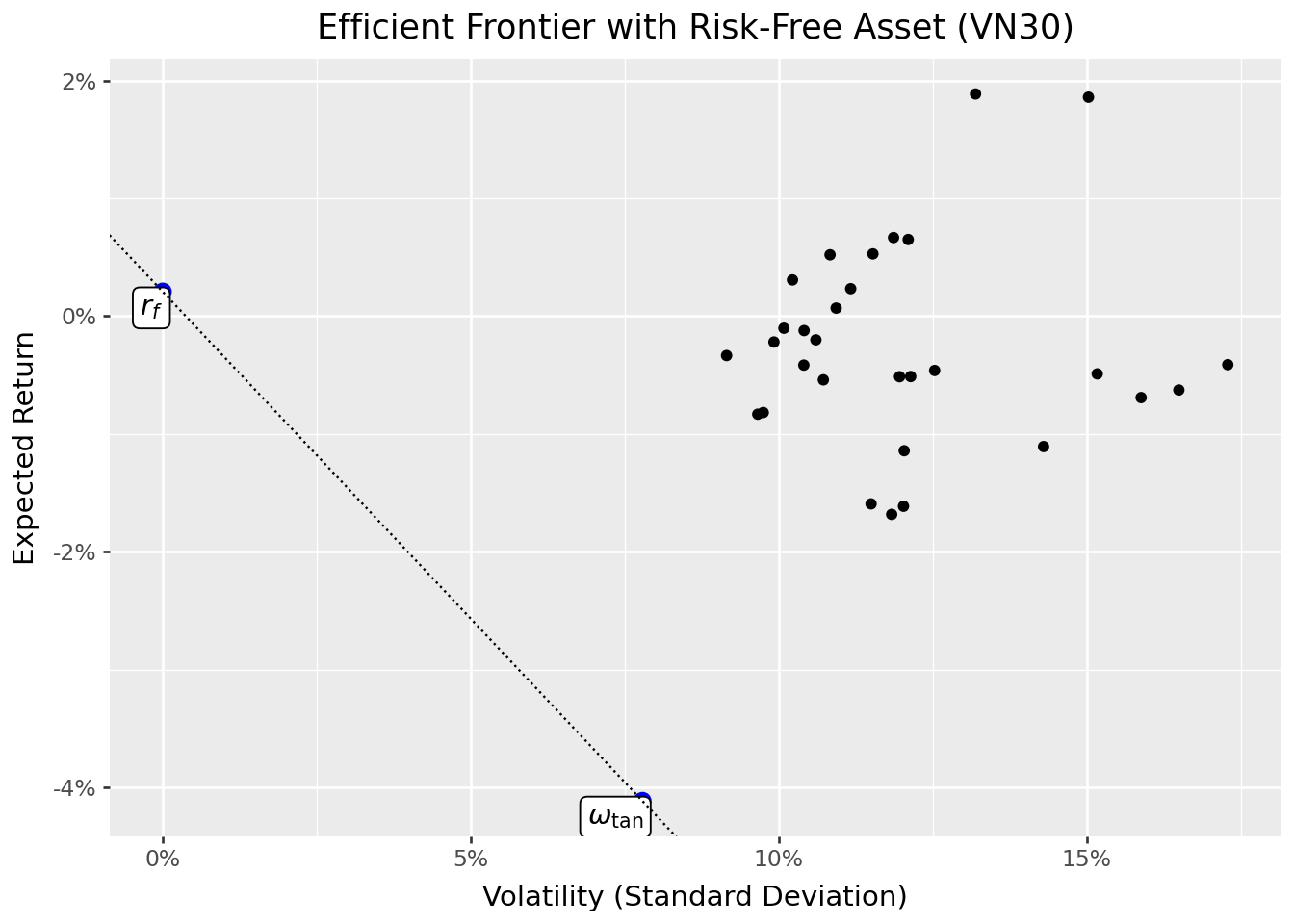
You may notice that estimated expected returns appear quite low, some even negative. This is not a model failure but reflects the realities of estimation:
Sample period matters: If the estimation window includes market downturns (such as the 2022-2023 period), realized average returns can be near zero or negative. Mean-variance optimization takes sample means literally.
Estimation noise in emerging markets: With volatile emerging market data, sample means are dominated by noise. A few extremely bad months can push the average below the risk-free rate even if the long-run equity premium is positive.
This highlights a fundamental challenge in portfolio optimization: the inputs we observe (historical returns) are noisy estimates of the true parameters we need (expected future returns).
16.6 The CAPM Equation: Risk and Expected Return
16.6.1 From Individual Optimization to Market Equilibrium
So far, we’ve focused on one investor’s optimization problem. The CAPM’s power comes from considering what happens when all investors optimize simultaneously.
If all investors follow mean-variance optimization, they all hold some combination of the risk-free asset and the tangency portfolio. The only difference between investors is their risk tolerance. More risk-averse investors hold more of the risk-free asset, while risk-tolerant investors may even borrow at the risk-free rate to leverage their position in the tangency portfolio.
16.6.2 The Market Portfolio
In equilibrium, the total demand for each risky asset must equal its supply. Since all investors hold the same portfolio of risky assets (the tangency portfolio), the equilibrium portfolio weights must equal the market capitalization weights. The tangency portfolio is the market portfolio.
This insight has enormous practical implications: instead of estimating expected returns and covariances to compute the tangency portfolio, we can simply use the market portfolio (approximated by a broad market index) as a proxy.
16.6.3 Deriving the CAPM Equation
From the first-order conditions of the optimization problem, we derived that:
\[ \tilde{\mu} = \frac{2}{\lambda}\Sigma\omega^* \]
Since \(\omega^*\) is proportional to \(\omega_{\text{tan}}\), and in equilibrium \(\omega_{\text{tan}}\) equals the market portfolio \(\omega_m\):
\[ \tilde{\mu} = c \cdot \Sigma\omega_m \]
for some constant \(c\). The \(i\)-th element of \(\Sigma\omega_m\) is:
\[ \sum_{j=1}^N \sigma_{ij}\omega_{m,j} = \text{Cov}(r_i, r_m) \]
where \(r_m = \sum_j \omega_{m,j} r_j\) is the return on the market portfolio.
For the market portfolio itself:
\[ \tilde{\mu}_m = c \cdot \text{Var}(r_m) = c \cdot \sigma_m^2 \]
Therefore \(c = \tilde{\mu}_m / \sigma_m^2\), and for any asset \(i\):
\[ \tilde{\mu}_i = \frac{\tilde{\mu}_m}{\sigma_m^2} \text{Cov}(r_i, r_m) = \beta_i \tilde{\mu}_m \]
where:
\[ \beta_i = \frac{\text{Cov}(r_i, r_m)}{\text{Var}(r_m)} \]
This is the famous CAPM equation:
\[ E(r_i) - r_f = \beta_i [E(r_m) - r_f] \]
16.6.4 Interpreting Beta
Beta (\(\beta_i\)) measures an asset’s systematic risk (i.e., its sensitivity to market movements). The interpretation is straightforward:
- \(\beta = 1\): The asset moves one-for-one with the market (average systematic risk)
- \(\beta > 1\): The asset amplifies market movements (aggressive, high systematic risk)
- \(\beta < 1\): The asset dampens market movements (defensive, low systematic risk)
- \(\beta < 0\): The asset moves opposite to the market (provides insurance)
The CAPM says that expected excess return is proportional to beta, not to total volatility. This explains why:
- An asset with zero beta earns only the risk-free rate (i.e., its risk is entirely idiosyncratic).
- An asset with beta of 1 earns the market risk premium
- A negative-beta asset earns less than the risk-free rate (i.e., investors pay for its insurance properties).
16.7 The Security Market Line
The CAPM predicts a linear relationship between beta and expected return. This relationship is called the Security Market Line (SML):
\[ E(r_i) = r_f + \beta_i [E(r_m) - r_f] \]
Unlike the Capital Market Line (which plots expected return against total risk), the Security Market Line plots expected return against systematic risk (beta).
betas = (sigma @ w_tan) / (w_tan.T @ sigma @ w_tan)
assets["beta"] = betas.values

price_of_risk = float(w_tan.T @ mu - rf)

assets_figure = (
    ggplot(assets, aes(x="beta", y="mu"))
    + geom_point()
    + geom_abline(intercept=rf, slope=price_of_risk)
    + scale_y_continuous(labels=percent_format())
    + labs(
        x="Beta (Systematic Risk)",
        y="Expected Return",
        title="Security Market Line"
    )
    + annotate("text", x=0.05, y=rf + 0.001, label="Risk-free rate")
)

assets_figure.show()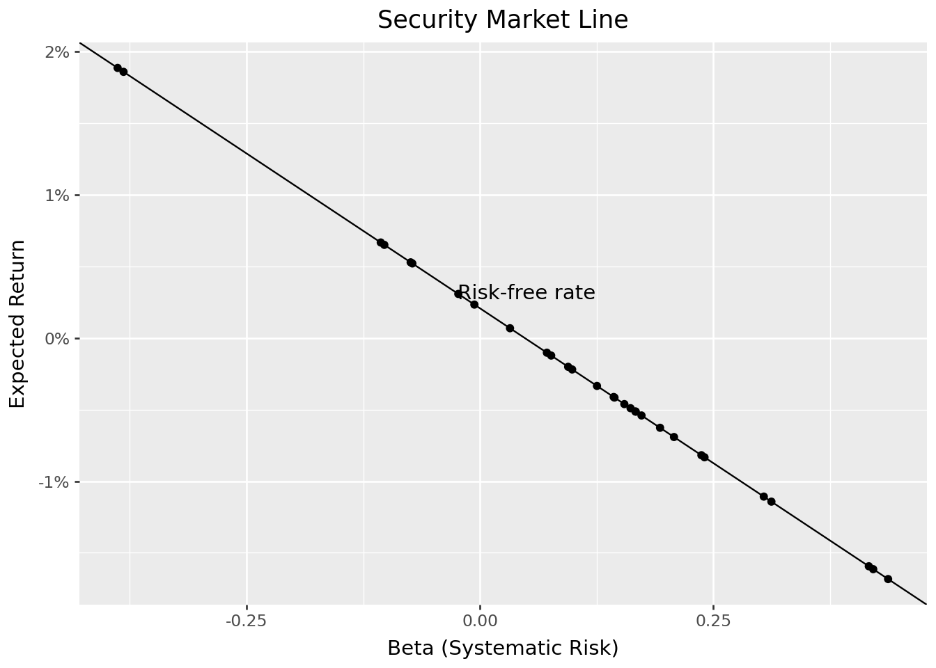
You may observe that the estimated SML has a negative slope, which seems to contradict CAPM’s prediction. This reflects a negative estimated market risk premium in our sample period (i.e., the market portfolio earned less than the risk-free rate).
When the market risk premium is negative, CAPM predicts that high-beta stocks should have lower expected returns than low-beta stocks. This is not a model failure, the model is behaving consistently. Rather, it reflects an unusual (but not impossible) sample period where risky assets underperformed safe assets.
This observation highlights an important distinction: CAPM describes expected returns in equilibrium, but realized returns over any particular period may differ substantially from expectations due to shocks and surprises.
16.8 Empirical Estimation of CAPM Parameters
16.8.1 The Regression Framework
In practice, we estimate CAPM parameters using time-series regression. The model implies:
\[ r_{i,t} - r_{f,t} = \alpha_i + \beta_i(r_{m,t} - r_{f,t}) + \varepsilon_{i,t} \]
where:
- \(r_{i,t}\): Return on asset \(i\) at time \(t\)
- \(r_{f,t}\): Risk-free rate at time \(t\)
- \(r_{m,t}\): Market return at time \(t\)
- \(\alpha_i\): Intercept (should be zero if CAPM holds)
- \(\beta_i\): Systematic risk (slope coefficient)
- \(\varepsilon_{i,t}\): Idiosyncratic shock (residual)
16.8.2 Alpha: Risk-Adjusted Performance
The intercept \(\alpha_i\) measures risk-adjusted performance. If CAPM holds perfectly, alpha should be zero for all assets (i.e., any excess return is exactly compensated by systematic risk).
- \(\alpha > 0\): The asset outperformed its CAPM-predicted return (positive abnormal return)
- \(\alpha < 0\): The asset underperformed its CAPM-predicted return (negative abnormal return)
Positive alpha is the holy grail of active management: earning returns beyond what systematic risk exposure would justify.
16.8.3 Loading Factor Data
We use Fama-French market excess returns as our market portfolio proxy. These data provide a widely accepted benchmark that is already adjusted for the risk-free rate:
import sqlite3

tidy_finance = sqlite3.connect(database="data/tidy_finance_python.sqlite")

factors = pd.read_sql_query(
    sql="SELECT date, smb, hml, rmw, cma, mkt_excess FROM factors_ff5_monthly",
    con=tidy_finance,
    parse_dates={"date"}
)

factors.head(3)| date | smb | hml | rmw | cma | mkt_excess | |
|---|---|---|---|---|---|---|
| 0 | 2011-07-31 | -0.015907 | -0.002812 | 0.060525 | 0.045291 | -0.078748 |
| 1 | 2011-08-31 | -0.061842 | 0.006189 | -0.022700 | -0.023177 | 0.029906 |
| 2 | 2011-09-30 | 0.014387 | 0.024301 | -0.006005 | 0.003588 | -0.002173 |
16.8.4 Running the Regressions
We estimate CAPM regressions for each stock in our universe:
import statsmodels.formula.api as smf

returns_excess_monthly = (returns_monthly
    .merge(factors, on="date", how="left")
    .assign(ret_excess=lambda x: x["ret"] - x["risk_free"])
)


def estimate_capm(data):
    model = smf.ols("ret_excess ~ mkt_excess", data=data).fit()
    result = pd.DataFrame({
        "coefficient": ["alpha", "beta"],
        "estimate": model.params.values,
        "t_statistic": model.tvalues.values
    })
    return result


capm_results = (returns_excess_monthly
    .groupby("symbol", group_keys=True)
    .apply(estimate_capm)
    .reset_index()
)

capm_results.head(4)| symbol | level_1 | coefficient | estimate | t_statistic | |
|---|---|---|---|---|---|
| 0 | ACB | 0 | alpha | -0.000826 | -0.105475 |
| 1 | ACB | 1 | beta | 0.604653 | 4.575750 |
| 2 | BCM | 0 | alpha | 0.035093 | 2.368668 |
| 3 | BCM | 1 | beta | 1.032462 | 4.581461 |
16.8.5 Visualizing Alpha Estimates
Figure 16.2 shows the estimated alphas across our VN30 sample. Statistical significance (at the 95% level) is indicated by color.
alphas = (capm_results
    .query("coefficient == 'alpha'")
    .assign(is_significant=lambda x: np.abs(x["t_statistic"]) >= 1.96)
)

alphas["symbol"] = pd.Categorical(
    alphas["symbol"],
    categories=alphas.sort_values("estimate")["symbol"],
    ordered=True
)

alphas_figure = (
    ggplot(alphas, aes(y="estimate", x="symbol", fill="is_significant"))
    + geom_col()
    + scale_y_continuous(labels=percent_format())
    + coord_flip()
    + labs(
        x="",
        y="Estimated Alpha (Monthly)",
        fill="Significant at 95%?",
        title="Estimated CAPM Alphas for VN30 Index Constituents"
    )
)

alphas_figure.show()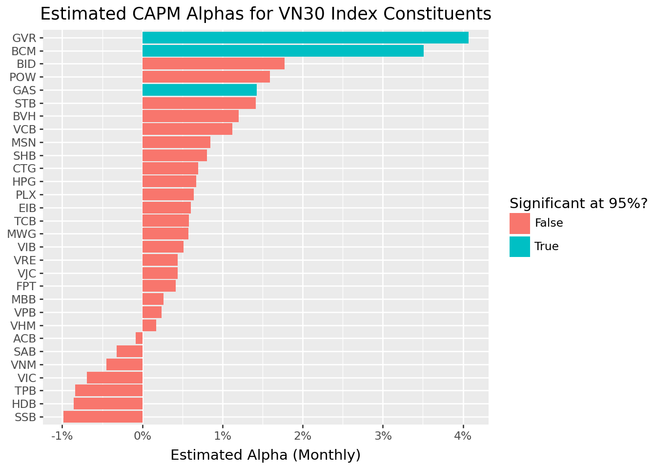
The distribution of alphas provides evidence on CAPM’s empirical validity. If the model holds, we expect:
- Most alphas close to zero
- Few statistically significant alphas
- Roughly equal numbers of positive and negative alphas
Systematic patterns in alphas, such as consistently positive alphas for certain types of stocks, would suggest the CAPM is incomplete and that additional risk factors may be needed.
16.9 Limitations and Extensions
16.9.1 The Market Portfolio Problem
A fundamental challenge in testing the CAPM is identifying the market portfolio. The theory requires a portfolio that includes all investable assets, not just stocks, but also bonds, real estate, private businesses, human capital, and even intangible assets. In practice, we use proxies like broad market indices (VNI, S&P 500), but these capture only publicly traded equities.
This limitation is profound. As Richard Roll famously argued, the CAPM is essentially untestable because the true market portfolio is unobservable. Any test of the CAPM is simultaneously a test of whether our proxy adequately represents the market.
16.9.2 Time-Varying Betas
The CAPM assumes that betas are constant over time, but this assumption rarely holds in practice. Companies undergo changes that affect their market sensitivity:
- Capital structure changes: Increasing leverage raises beta
- Business model evolution: Diversification into new industries can alter systematic risk
- Market conditions: Betas often increase during market stress
Conditional CAPM models (Jagannathan and Wang 1996) address this by allowing risk premiums and betas to vary with the business cycle.
16.9.3 Empirical Anomalies
Decades of empirical research have documented patterns in stock returns that CAPM cannot explain:
- Size effect: Small-cap stocks tend to outperform large-cap stocks, even after adjusting for beta
- Value effect: Stocks with high book-to-market ratios outperform growth stocks
- Momentum: Stocks that performed well recently tend to continue performing well
These anomalies suggest that systematic risk has multiple dimensions beyond market exposure.
16.9.4 Multifactor Extensions
The limitations of CAPM have led to increasingly sophisticated asset pricing models. The Fama-French three-factor model (Fama and French 1992) adds two factors to capture size and value effects:
- SMB (Small Minus Big): Returns on small stocks minus large stocks
- HML (High Minus Low): Returns on value stocks minus growth stocks
The Fama-French five-factor model (Fama and French 2015) adds two more dimensions:
- RMW (Robust Minus Weak): Returns on profitable firms minus unprofitable firms
- CMA (Conservative Minus Aggressive): Returns on conservative investors minus aggressive investors
The Carhart four-factor model (Carhart 1997) adds momentum to the three-factor framework.
Other theoretical developments include:
- Consumption CAPM: Links asset prices to macroeconomic consumption risk
- Q-factor model (Hou, Xue, and Zhang 2014): Derives factors from investment-based asset pricing theory
- Arbitrage Pricing Theory: Allows for multiple sources of systematic risk without specifying their identity
Despite its limitations, the CAPM remains valuable as a conceptual benchmark. Its core insight (i.e., only systematic, undiversifiable risk commands a premium) continues to inform how we think about risk and return.
16.10 Key Takeaways
This chapter introduced the Capital Asset Pricing Model and its implications for understanding the relationship between risk and expected return. The main insights are:
Not all risk is rewarded: The CAPM distinguishes between systematic risk (which cannot be diversified away and commands a premium) and idiosyncratic risk (which can be eliminated through diversification and earns no premium).
The tangency portfolio is universal: When a risk-free asset exists, all mean-variance investors hold the same portfolio of risky assets (i.e., the tangency or maximum Sharpe ratio portfolio). They differ only in how much they allocate to this portfolio versus the risk-free asset.
In equilibrium, the tangency portfolio is the market portfolio: Since all investors hold the same risky portfolio, and total demand must equal supply, the equilibrium portfolio weights are market capitalization weights.
Expected returns depend on beta: The CAPM equation states that expected excess return equals beta times the market risk premium. Beta measures covariance with the market portfolio, normalized by market variance.
Alpha measures risk-adjusted performance: Positive alpha indicates returns above what systematic risk would justify; negative alpha indicates underperformance.
Empirical challenges exist: Testing the CAPM requires identifying the market portfolio, which is unobservable in practice. Documented anomalies (size, value, momentum) suggest additional risk factors beyond market exposure.
Extensions abound: Multifactor models like Fama-French extend the CAPM framework by adding factors that capture dimensions of systematic risk the market factor misses.
The CAPM’s elegance lies in its simplicity: a single factor (i.e., exposure to the market) should explain expected returns in equilibrium. While reality is more complex, this framework provides the foundation for all modern asset pricing theory.