31  Standardized Earnings Surprises (SUE)

In the context of the Ho Chi Minh Stock Exchange (HOSE) and the Hanoi Stock Exchange (HNX), earnings announcements represent critical information events. Investors and quantitative analysts continuously monitor the deviation between reported earnings and market expectations. This deviation is quantified as the Standardized Earnings Surprise (SUE).

This chapter details the methodology for calculating SUE using three distinct approaches frequently utilized in academic literature and institutional research. We apply these methods to a dataset of Vietnamese large-cap equities to illustrate the mechanics of the calculation. The goal is to isolate the “surprise” component of earnings, which is a known predictor of post-earnings announcement drift (PEAD) (Bernard and Thomas 1989; Livnat and Mendenhall 2006).

31.1 Methodology

We define three primary methods for calculating SUE. Each method differs in how it establishes the “expected” earnings value.

31.1.1 Method 1: Seasonal Random Walk

This method assumes that earnings follow a seasonal pattern. The best predictor for the current quarter’s earnings per share (EPS) is the EPS from the same quarter in the previous year. This controls for the seasonality often seen in Vietnamese sectors like retail and agriculture.

\[SUE_{1} = \frac{EPS_{t} - EPS_{t-4}}{P_{t}}\]

Where:

• \(EPS_{t}\) is the current quarterly Earnings Per Share.

• \(EPS_{t-4}\) is the Earnings Per Share from the same quarter of the prior fiscal year.

• \(P_{t}\) is the stock price at the end of the quarter (used as a deflator).

31.1.2 Method 2: Exclusion of Special Items

Reported earnings often contain non-recurring items (e.g., asset sales, one-time write-offs) that distort the true operating performance. This method adjusts the reported EPS by removing the after-tax impact of special items.

In Vietnam, the standard Corporate Income Tax (CIT) rate is generally 20%. We adjust special items to reflect their impact on net income.

\[ Adjusted \ EPS = Reported \ EPS - \frac{Special \ Items \times (1 - CIT)}{Shares \ Outstanding} \]

The SUE calculation then follows the seasonal logic but uses the adjusted EPS figures: \[SUE_{2} = \frac{Adj \ EPS_{t} - Adj \ EPS_{t-4}}{P_{t}}\]

31.1.3 Method 3: Analyst Consensus

This method relies on market consensus rather than historical time series. It compares the actual reported earnings against the median analyst forecast provided prior to the announcement.

\[SUE_{3} = \frac{Actual \ EPS - Median \ Estimate}{P_{t}}\]

Whether the consensus is the right expectation, and when a machine-learning correction of it is better, is the subject of Chapter 32.

31.2 Data Description

For this analysis, we utilize a dataset covering the fiscal years 2023 through 2025. The data includes quarterly financial statements and analyst consensus estimates for a selection of VN30 index constituents.

The dataset, vietnam_fin_data.csv, contains the following columns:

• ticker: Stock symbol (e.g., VNM, VCB, HPG).

• fiscal_year: The financial year.

• fiscal_qtr: The financial quarter (1-4).

• eps_basic: Basic Earnings Per Share (VND).

• price_close: Closing price at quarter end (VND).

• special_items: Pre-tax special items value (VND millions). (i.e., is_other_profit in DataCore).

• shares_out: Shares outstanding (millions).

• analyst_med: Median analyst EPS estimate (VND).

31.2.1 Visualizing the Core Data

Below is a tabular representation of the raw data we have ingested for the analysis.

ticker	fiscal_year	fiscal_qtr	eps_basic	price_close	special_items	shares_out	analyst_med
VNM	2023	1	1200	68000	0	2090	1150
VNM	2023	2	1350	71000	50000	2090	1300
VNM	2023	3	1400	74000	0	2090	1450
VNM	2023	4	1100	69000	-20000	2090	1150
VNM	2024	1	1300	72000	0	2090	1250
VNM	2024	2	1500	75000	0	2090	1400
VCB	2023	1	1800	85000	10000	5500	1700
VCB	2024	1	2100	92000	0	5500	2000

31.3 Implementation

31.3.1 Python Setup and Data Loading

First, we establish our environment and load the dataset. We ensure the data is sorted by ticker and time to allow for accurate lag calculations.

import pandas as pd
import numpy as np
import matplotlib.pyplot as plt

# Creating the dataset directly for this chapter's demonstration
data = {
    'ticker': ['VNM']*8 + ['VCB']*8 + ['HPG']*8,
    'fiscal_year': [2023, 2023, 2023, 2023, 2024, 2024, 2024, 2024] * 3,
    'fiscal_qtr': [1, 2, 3, 4, 1, 2, 3, 4] * 3,
    'eps_basic': [
        1200, 1350, 1400, 1100, 1300, 1500, 1450, 1250, # VNM
        1800, 1900, 2000, 2200, 2100, 2300, 2400, 2600, # VCB
        500, 600, 550, 400, 700, 800, 750, 600          # HPG
    ],
    'price_close': [
        68000, 71000, 74000, 69000, 72000, 75000, 73000, 70000, # VNM
        85000, 88000, 90000, 95000, 92000, 96000, 98000, 102000, # VCB
        20000, 22000, 21000, 19000, 25000, 28000, 27000, 24000 # HPG
    ],
    'special_items': [
        0, 50000, 0, -20000, 0, 0, 10000, 0, # VNM (VND Millions)
        10000, 0, 0, 50000, 0, 20000, 0, 0, # VCB
        0, 0, -50000, 0, 100000, 0, 0, 0 # HPG
    ],
    'shares_out': [2090]*8 + [5580]*8 + [5810]*8, # In Millions
    'analyst_med': [
        1150, 1300, 1450, 1150, 1250, 1400, 1480, 1200, # VNM
        1700, 1850, 1950, 2150, 2000, 2250, 2450, 2550, # VCB
        450, 550, 600, 450, 650, 750, 800, 650 # HPG
    ]
}

df = pd.DataFrame(data)

# Sort strictly to ensure shift operations work on correct temporal sequence
df = df.sort_values(by=['ticker', 'fiscal_year', 'fiscal_qtr'])
print(df.head())

   ticker  fiscal_year  fiscal_qtr  eps_basic  price_close  special_items  \
16    HPG         2023           1        500        20000              0   
17    HPG         2023           2        600        22000              0   
18    HPG         2023           3        550        21000         -50000   
19    HPG         2023           4        400        19000              0   
20    HPG         2024           1        700        25000         100000   

    shares_out  analyst_med  
16        5810          450  
17        5810          550  
18        5810          600  
19        5810          450  
20        5810          650  

31.3.2 Calculation Logic

We now apply the functions to calculate the three variations of SUE.

Step 1: Handling Seasonality (Lags)

For Methods 1 and 2, we require the data from the same quarter of the previous year (lag 4).

# Group by ticker to ensure we don't shift data between companies
df['eps_lag4'] = df.groupby('ticker')['eps_basic'].shift(4)

Step 2: Adjusting for Special Items

For Method 2, we must strip out non-recurring items. We apply the Vietnamese Corporate Income Tax (CIT) rate of 20%.

The formula for the adjustment per share is: \[ \text{Adjustment} = \frac{\text{Special Items} \times (1 - 0.20)}{\text{Shares Outstanding}} \]

# Constants
CIT_RATE_VN = 0.20

# Calculate impact per share
# Note: special_items are in millions, shares_out are in millions
# The units cancel out, leaving the result in VND per share.
df['spi_impact_per_share'] = (df['special_items'] * (1 - CIT_RATE_VN)) / df['shares_out']

# Calculate Adjusted EPS
df['eps_adjusted'] = df['eps_basic'] - df['spi_impact_per_share']

# Create lag for Adjusted EPS
df['eps_adj_lag4'] = df.groupby('ticker')['eps_adjusted'].shift(4)

Step 3: Computing SUE Variants

We finalize the calculation by computing the difference between actual (or adjusted) and expected values, deflated by the stock price.

# Method 1: Seasonal Random Walk (Standard EPS)
df['sue_1'] = (df['eps_basic'] - df['eps_lag4']) / df['price_close']

# Method 2: Seasonal Random Walk (Excluding Special Items)
df['sue_2'] = (df['eps_adjusted'] - df['eps_adj_lag4']) / df['price_close']

# Method 3: Analyst Forecasts (IBES Equivalent)
df['sue_3'] = (df['eps_basic'] - df['analyst_med']) / df['price_close']

# Scaling for readability (converting to percentage)
df['sue_1_pct'] = df['sue_1'] * 100
df['sue_2_pct'] = df['sue_2'] * 100
df['sue_3_pct'] = df['sue_3'] * 100

31.4 Results and Analysis

We present the calculated standardized earnings surprises for the fiscal year 2024. Positive values indicate a positive surprise (beating expectations), while negative values indicate a miss.

31.4.1 Tabular Results (FY 2024)

# Filter for 2024 results where lag data exists
results_2024 = df[df['fiscal_year'] == 2024][['ticker', 'fiscal_qtr', 'sue_1_pct', 'sue_2_pct', 'sue_3_pct']]

# Display formatted table
from IPython.display import display, Markdown
markdown_table = results_2024.to_markdown(index=False, floatfmt=".4f")
display(Markdown(markdown_table))

ticker	fiscal_qtr	sue_1_pct	sue_2_pct	sue_3_pct
HPG	1	0.8000	0.7449	0.2000
HPG	2	0.7143	0.7143	0.1786
HPG	3	0.7407	0.7152	-0.1852
HPG	4	0.8333	0.8333	-0.2083
VCB	1	0.3261	0.3276	0.1087
VCB	2	0.4167	0.4137	0.0521
VCB	3	0.4082	0.4082	-0.0510
VCB	4	0.3922	0.3992	0.0490
VNM	1	0.1389	0.1389	0.0694
VNM	2	0.2000	0.2255	0.1333
VNM	3	0.0685	0.0632	-0.0411
VNM	4	0.2143	0.2033	0.0714

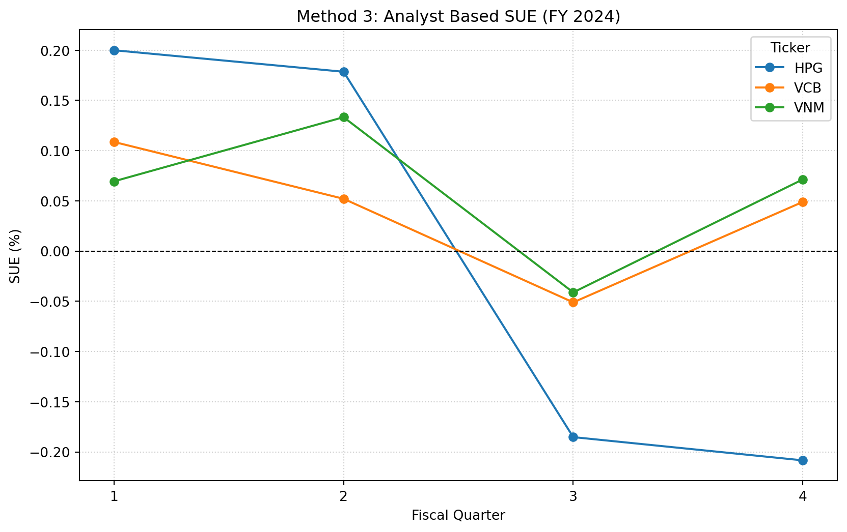
31.4.2 Visualization

The following figure plots the Analyst-based SUE (Method 3) for the selected tickers over the 2024 fiscal year.

pivot_sue = results_2024.pivot(index='fiscal_qtr', columns='ticker', values='sue_3_pct')

plt.figure(figsize=(10, 6))
for column in pivot_sue.columns:
    plt.plot(pivot_sue.index, pivot_sue[column], marker='o', label=column)

plt.title('Method 3: Analyst Based SUE (FY 2024)')
plt.xlabel('Fiscal Quarter')
plt.ylabel('SUE (%)')
plt.axhline(0, color='black', linestyle='--', linewidth=0.8)
plt.legend(title='Ticker')
plt.grid(True, linestyle=':', alpha=0.6)
plt.xticks([1, 2, 3, 4])
plt.show()

Figure 31.1

31.5 Conclusion

In this chapter, we have formalized the calculation of Standardized Earnings Surprises for the Vietnamese market. We demonstrated that relying solely on raw EPS growth (Method 1) can be misleading in the presence of non-recurring items. Furthermore, analyst-based surprises (Method 3) often provide a cleaner signal of new information reaching the market.

For robust quantitative modeling in Vietnam, we recommend using Method 2 when analyst data is sparse (common in small-cap stocks) and Method 3 for VN30 constituents where analyst coverage is deep and liquid.

Bernard, Victor L, and Jacob K Thomas. 1989. “Post-Earnings-Announcement Drift: Delayed Price Response or Risk Premium?” Journal of Accounting Research 27: 1–36. https://doi.org/10.2307/2491062.

Livnat, Joshua, and Richard R Mendenhall. 2006. “Comparing the Post–Earnings Announcement Drift for Surprises Calculated from Analyst and Time Series Forecasts.” Journal of Accounting Research 44 (1): 177–205.