import pandas as pd
import numpy as np
import sqlite3
from datetime import datetime
from io import BytesIO

from plotnine import *
from mizani.formatters import comma_format, percent_format3 Datacore Data
This chapter introduces Datacore, Vietnam’s data platform for academic, corporate, and government research. Datacore provides comprehensive financial and economic datasets, including historical trading data, company fundamentals, and macroeconomic indicators essential for reproducible finance research. We use Datacore as the primary data source throughout this book.
3.1 Data Access Options
Readers can access the data used in this book through several channels:
Institutional subscription: Many universities and research institutions subscribe to Datacore. Check with your library or research office for access credentials. If your institution does not yet have a subscription, consider requesting one through your library’s acquisition process—Datacore offers institutional pricing for academic use.
Demo datasets: Datacore provides demo datasets that allow you to run the code examples in this book with sample data.
3.2 Chapter Overview
The chapter is organized as follows. We first establish the connection to Datacore’s cloud storage infrastructure. Then, we download and prepare company fundamentals data, including balance sheet items, income statement variables, and derived metrics essential for asset pricing research. Next, we retrieve and process stock price data, computing returns, market capitalizations, and excess returns. We conclude by merging these datasets and providing descriptive statistics that characterize the Vietnamese equity market.
3.3 Setting Up the Environment
We begin by loading the Python packages used throughout this chapter. The core packages include pandas for data manipulation, numpy for numerical operations, and sqlite3 for local database management. We also import visualization libraries for creating publication-quality figures.
We establish a connection to our local SQLite database, which serves as the central repository for all processed data. This database was introduced in the previous chapter and will store the cleaned datasets for use in subsequent analyses.
tidy_finance = sqlite3.connect(database="data/tidy_finance_python.sqlite")We define the date range for our data collection. The Vietnamese stock market began operations in July 2000 with the establishment of the Ho Chi Minh City Stock Exchange (HOSE), so our sample period starts from 2000 and extends through the end of 2024.
start_date = "2000-01-01"
end_date = "2024-12-31"
3.4 Connecting to Datacore
Datacore delivers data through a cloud-based object storage system built on MinIO, an S3-compatible storage infrastructure. This architecture enables efficient, programmatic access to large datasets without the limitations of traditional database connections. To access the data, you need credentials provided by Datacore upon subscription: an endpoint URL, access key, and secret key.
The following class establishes the connection to Datacore’s storage system. The credentials are stored as environment variables for security, following best practices for credential management in research computing environments.
import os
import boto3
from botocore.client import Config

class DatacoreConnection:
    """
    Connection handler for Datacore's MinIO-based storage system.

    This class manages authentication and provides methods for
    accessing financial datasets stored in Datacore's cloud infrastructure.

    Attributes
    ----------
    s3 : boto3.client
        S3-compatible client for interacting with Datacore storage
    """

    def __init__(self):
        """Initialize connection using environment variables."""
        self.MINIO_ENDPOINT = os.environ["MINIO_ENDPOINT"]
        self.MINIO_ACCESS_KEY = os.environ["MINIO_ACCESS_KEY"]
        self.MINIO_SECRET_KEY = os.environ["MINIO_SECRET_KEY"]
        self.REGION = os.getenv("MINIO_REGION", "us-east-1")

        self.s3 = boto3.client(
            "s3",
            endpoint_url=self.MINIO_ENDPOINT,
            aws_access_key_id=self.MINIO_ACCESS_KEY,
            aws_secret_access_key=self.MINIO_SECRET_KEY,
            region_name=self.REGION,
            config=Config(signature_version="s3v4"),
        )

    def test_connection(self):
        """Verify connection by listing available buckets."""
        response = self.s3.list_buckets()
        print("Connected successfully. Available buckets:")
        for bucket in response.get("Buckets", []):
            print(f"  - {bucket['Name']}")

    def list_objects(self, bucket_name, prefix=""):
        """List objects in a bucket with optional prefix filter."""
        response = self.s3.list_objects_v2(
            Bucket=bucket_name,
            Prefix=prefix
        )
        return [obj["Key"] for obj in response.get("Contents", [])]

    def read_excel(self, bucket_name, key):
        """Read an Excel file from Datacore storage."""
        obj = self.s3.get_object(Bucket=bucket_name, Key=key)
        return pd.read_excel(BytesIO(obj["Body"].read()))

    def read_csv(self, bucket_name, key, **kwargs):
        """Read a CSV file from Datacore storage."""
        obj = self.s3.get_object(Bucket=bucket_name, Key=key)
        return pd.read_csv(BytesIO(obj["Body"].read()), **kwargs)
With the connection class defined, we can establish a connection and verify access to Datacore’s data repositories.
# Initialize connection
conn = DatacoreConnection()
conn.test_connection()

# Get bucket name from environment
bucket_name = os.environ["MINIO_BUCKET"]
Connected successfully. Available buckets:
- dsteam-data
- rawbctc3.5 Company Fundamentals Data
Firm accounting data are essential for portfolio analyses, factor construction, and valuation studies. Datacore hosts comprehensive fundamentals data for Vietnamese listed companies, including annual and quarterly financial statements prepared according to Vietnamese Accounting Standards (VAS).
3.5.1 Understanding Vietnamese Financial Statements
Before processing the data, it is important to understand the structure of Vietnamese financial reports. Vietnamese companies follow VAS, which shares similarities with International Financial Reporting Standards (IFRS) but has notable differences:
Fiscal Year: Most Vietnamese companies use a calendar fiscal year ending December 31, though some companies (particularly in retail and agriculture) use different fiscal year-ends.
Reporting Frequency: Listed companies must publish quarterly financial statements within 20 days of quarter-end and annual audited statements within 90 days of fiscal year-end.
Industry-Specific Formats: Companies in banking, insurance, and securities sectors follow specialized reporting formats that differ from the standard industrial format.
Currency: All figures are reported in Vietnamese Dong (VND). Given the large nominal values (millions to trillions of VND), we often scale figures to millions or billions for readability.
3.5.2 Downloading Fundamentals Data
Datacore organizes fundamentals data in Excel files partitioned by time period for efficient access. We download and concatenate these files to create a comprehensive dataset spanning our sample period.
# Define paths to fundamentals data files
fundamentals_paths = [
    "fundamental_annual_1767674486317/fundamental_annual_1.xlsx",
    "fundamental_annual_1767674486317/fundamental_annual_2.xlsx",
    "fundamental_annual_1767674486317/fundamental_annual_3.xlsx",
]

# Download and combine all files
fundamentals_list = []
for path in fundamentals_paths:
    df_temp = conn.read_excel(bucket_name, path)
    fundamentals_list.append(df_temp)
    print(f"Downloaded: {path} ({len(df_temp):,} rows)")

df_fundamentals_raw = pd.concat(fundamentals_list, ignore_index=True)
print(f"\nTotal observations: {len(df_fundamentals_raw):,}")
/home/mikenguyen/project/tidyfinance/.venv/lib/python3.13/site-packages/openpyxl/styles/stylesheet.py:237: UserWarning: Workbook contains no default style, apply openpyxl's defaultDownloaded: fundamental_annual_1767674486317/fundamental_annual_1.xlsx (10,000 rows)/home/mikenguyen/project/tidyfinance/.venv/lib/python3.13/site-packages/openpyxl/styles/stylesheet.py:237: UserWarning: Workbook contains no default style, apply openpyxl's defaultDownloaded: fundamental_annual_1767674486317/fundamental_annual_2.xlsx (10,000 rows)/home/mikenguyen/project/tidyfinance/.venv/lib/python3.13/site-packages/openpyxl/styles/stylesheet.py:237: UserWarning: Workbook contains no default style, apply openpyxl's defaultDownloaded: fundamental_annual_1767674486317/fundamental_annual_3.xlsx (2,821 rows)
Total observations: 22,8213.5.3 Cleaning and Standardizing Fundamentals
The raw fundamentals data requires several cleaning steps to ensure consistency and usability. We standardize variable names, handle missing values, and create derived variables commonly used in asset pricing research.
def clean_fundamentals(df):
    """
    Clean and standardize company fundamentals data.

    Parameters
    ----------
    df : pd.DataFrame
        Raw fundamentals data from Datacore

    Returns
    -------
    pd.DataFrame
        Cleaned fundamentals with standardized column names
    """
    df = df.copy()

    # Standardize identifiers
    df["symbol"] = df["symbol"].astype(str).str.upper().str.strip()
    df["year"] = pd.to_numeric(df["year"], errors="coerce").astype("Int64")

    # Drop rows with missing identifiers
    df = df.dropna(subset=["symbol", "year"])

    # Define columns that should be numeric
    numeric_columns = [
        "total_asset", "total_equity", "total_liabilities",
        "total_current_asset", "total_current_liabilities",
        "is_net_revenue", "is_cogs", "is_manage_expense",
        "is_interest_expense", "is_eat", "is_net_business_profit",
        "na_tax_deferred", "nl_tax_deferred", "e_preferred_stock",
        "capex", "total_cfo", "ca_cce", "ca_total_inventory",
        "ca_acc_receiv", "cfo_interest_expense", "basic_eps",
        "is_shareholders_eat", "cl_loan", "cl_finlease",
        "cl_due_long_debt", "nl_loan", "nl_finlease",
        "is_cos_of_sales", "e_equity"
    ]

    for col in numeric_columns:
        if col in df.columns:
            df[col] = pd.to_numeric(df[col], errors="coerce")

    # Handle duplicates: keep row with most non-missing values
    df["_completeness"] = df.notna().sum(axis=1)
    df = (df
        .sort_values(["symbol", "year", "_completeness"])
        .drop_duplicates(subset=["symbol", "year"], keep="last")
        .drop(columns="_completeness")
        .reset_index(drop=True)
    )

    return df

df_fundamentals = clean_fundamentals(df_fundamentals_raw)
print(f"After cleaning: {len(df_fundamentals):,} firm-year observations")
print(f"Unique firms: {df_fundamentals['symbol'].nunique():,}")
After cleaning: 21,232 firm-year observations
Unique firms: 1,5543.5.4 Creating Standardized Variables
To facilitate comparison with international studies and ensure compatibility with standard asset pricing methodologies, we create variables following conventions established in the academic literature. We map Vietnamese financial statement items to their Compustat equivalents where possible.
def create_standard_variables(df):
    """
    Create standardized financial variables for asset pricing research.

    This function maps Vietnamese financial statement items to standard
    variable names used in the academic finance literature, following
    conventions from Fama and French (1992, 1993, 2015).

    Parameters
    ----------
    df : pd.DataFrame
        Cleaned fundamentals data

    Returns
    -------
    pd.DataFrame
        Fundamentals with standardized variables added
    """
    df = df.copy()

    # Fiscal date (assume December year-end)
    df["datadate"] = pd.to_datetime(df["year"].astype(str) + "-12-31")

    # === Balance Sheet Items ===
    df["at"] = df["total_asset"]                    # Total assets
    df["lt"] = df["total_liabilities"]              # Total liabilities
    df["seq"] = df["total_equity"]                  # Stockholders' equity
    df["act"] = df["total_current_asset"]           # Current assets
    df["lct"] = df["total_current_liabilities"]     # Current liabilities

    # Common equity (fallback to total equity if not available)
    df["ceq"] = df.get("e_equity", df["seq"])

    # === Deferred Taxes ===
    df["txditc"] = df.get("na_tax_deferred", 0).fillna(0)  # Deferred tax assets
    df["txdb"] = df.get("nl_tax_deferred", 0).fillna(0)    # Deferred tax liab.
    df["itcb"] = 0  # Investment tax credit (rare in Vietnam)

    # === Preferred Stock ===
    pref = df.get("e_preferred_stock", 0)
    if isinstance(pref, pd.Series):
        pref = pref.fillna(0)
    df["pstk"] = pref
    df["pstkrv"] = pref  # Redemption value
    df["pstkl"] = pref   # Liquidating value

    # === Income Statement Items ===
    df["sale"] = df["is_net_revenue"]                        # Net sales/revenue
    df["cogs"] = df.get("is_cogs", 0).fillna(0)              # Cost of goods sold
    df["xsga"] = df.get("is_manage_expense", 0).fillna(0)    # SG&A expenses
    df["xint"] = df.get("is_interest_expense", 0).fillna(0)  # Interest expense
    df["ni"] = df.get("is_eat", np.nan)                      # Net income
    df["oibdp"] = df.get("is_net_business_profit", np.nan)   # Operating income

    # === Cash Flow Items ===
    df["oancf"] = df.get("total_cfo", np.nan)  # Operating cash flow
    df["capx"] = df.get("capex", np.nan)       # Capital expenditures

    return df

df_fundamentals = create_standard_variables(df_fundamentals)
3.5.5 Computing Book Equity and Profitability
Book equity is a crucial variable for value investing strategies and the construction of HML (High Minus Low) factor portfolios. We follow the definition from Kenneth French’s data library, which accounts for deferred taxes and preferred stock.
def compute_book_equity(df):
    """
    Compute book equity following Fama-French conventions.

    Book equity = Stockholders' equity
                  + Deferred taxes and investment tax credit
                  - Preferred stock

    Negative or zero book equity is set to missing, as book-to-market
    ratios are undefined for such firms.

    Parameters
    ----------
    df : pd.DataFrame
        Fundamentals with standardized variables

    Returns
    -------
    pd.DataFrame
        Fundamentals with book equity (be) added
    """
    df = df.copy()

    # Primary measure: stockholders' equity
    # Fallback 1: common equity + preferred stock
    # Fallback 2: total assets - total liabilities
    seq_measure = (df["seq"]
        .combine_first(df["ceq"] + df["pstk"])
        .combine_first(df["at"] - df["lt"])
    )

    # Add deferred taxes
    deferred_taxes = (df["txditc"]
        .combine_first(df["txdb"] + df["itcb"])
        .fillna(0)
    )

    # Subtract preferred stock (use redemption value as primary)
    preferred = (df["pstkrv"]
        .combine_first(df["pstkl"])
        .combine_first(df["pstk"])
        .fillna(0)
    )

    # Book equity calculation
    df["be"] = seq_measure + deferred_taxes - preferred

    # Set non-positive book equity to missing
    df["be"] = df["be"].where(df["be"] > 0, np.nan)

    return df

df_fundamentals = compute_book_equity(df_fundamentals)

# Summary statistics for book equity
print("Book Equity Summary Statistics (in million VND):")
print(df_fundamentals["be"].describe().round(2))
Book Equity Summary Statistics (in million VND):
count 2.023500e+04
mean 1.031884e+12
std 4.705269e+12
min 4.404402e+07
25% 7.267610e+10
50% 1.803885e+11
75% 5.304653e+11
max 1.836314e+14
Name: be, dtype: float64Operating profitability, introduced by Fama and French (2015), measures a firm’s profits relative to its book equity. Firms with higher operating profitability tend to have higher expected returns.
def compute_profitability(df):
    """
    Compute operating profitability following Fama-French (2015).

    Operating profitability = (Revenue - COGS - SG&A - Interest) / Book Equity

    Parameters
    ----------
    df : pd.DataFrame
        Fundamentals with book equity computed

    Returns
    -------
    pd.DataFrame
        Fundamentals with operating profitability (op) added
    """
    df = df.copy()

    # Operating profit before taxes
    operating_profit = (
        df["sale"]
        - df["cogs"].fillna(0)
        - df["xsga"].fillna(0)
        - df["xint"].fillna(0)
    )

    # Scale by book equity
    df["op"] = operating_profit / df["be"]

    # Winsorize extreme values (outside 1st and 99th percentiles)
    lower = df["op"].quantile(0.01)
    upper = df["op"].quantile(0.99)
    df["op"] = df["op"].clip(lower=lower, upper=upper)

    return df

df_fundamentals = compute_profitability(df_fundamentals)
3.5.6 Computing Investment
Investment, measured as asset growth, captures firms’ investment behavior. Fama and French (2015) document that firms with high asset growth (aggressive investment) tend to have lower future returns.
def compute_investment(df):
    """
    Compute investment (asset growth) following Fama-French (2015).

    Investment = (Total Assets_t / Total Assets_{t-1}) - 1

    Parameters
    ----------
    df : pd.DataFrame
        Fundamentals data

    Returns
    -------
    pd.DataFrame
        Fundamentals with investment (inv) added
    """
    df = df.copy()

    # Create lagged assets
    df_lag = (df[["symbol", "year", "at"]]
        .assign(year=lambda x: x["year"] + 1)
        .rename(columns={"at": "at_lag"})
    )

    # Merge lagged values
    df = df.merge(df_lag, on=["symbol", "year"], how="left")

    # Compute investment (asset growth)
    df["inv"] = df["at"] / df["at_lag"] - 1

    # Set to missing if lagged assets non-positive
    df["inv"] = df["inv"].where(df["at_lag"] > 0, np.nan)

    return df

df_fundamentals = compute_investment(df_fundamentals)
3.5.7 Computing Total Debt
In Vietnamese financial statements, total liabilities include non-interest-bearing items such as accounts payable and tax payables. For leverage analysis, we compute total interest-bearing debt by aggregating loan and lease obligations.
def compute_total_debt(df):
    """
    Compute total interest-bearing debt.

    Total Debt = Short-term loans + Finance leases (current)
                 + Current portion of long-term debt
                 + Long-term loans + Finance leases (non-current)

    Parameters
    ----------
    df : pd.DataFrame
        Fundamentals data

    Returns
    -------
    pd.DataFrame
        Fundamentals with total_debt added
    """
    df = df.copy()

    df["total_debt"] = (
        df.get("cl_loan", 0).fillna(0) +           # Short-term bank loans
        df.get("cl_finlease", 0).fillna(0) +       # Current finance leases
        df.get("cl_due_long_debt", 0).fillna(0) +  # Current portion LT debt
        df.get("nl_loan", 0).fillna(0) +           # Long-term bank loans
        df.get("nl_finlease", 0).fillna(0)         # Non-current finance leases
    )

    return df

df_fundamentals = compute_total_debt(df_fundamentals)
3.5.8 Applying Filters
We apply standard filters to ensure data quality: requiring positive assets, non-negative sales, and presence of core variables needed for portfolio construction.
# Keep only observations with required variables
required_vars = ["at", "lt", "seq", "sale"]
comp_vn = df_fundamentals.dropna(subset=required_vars)

# Apply quality filters
comp_vn = comp_vn.query("at > 0")      # Positive assets
comp_vn = comp_vn.query("sale >= 0")   # Non-negative sales

# Keep last observation per firm-year (in case of restatements)
comp_vn = (comp_vn
    .sort_values("datadate")
    .groupby(["symbol", "year"])
    .tail(1)
    .reset_index(drop=True)
)

# Diagnostic summary
print(f"Final sample: {len(comp_vn):,} firm-year observations")
print(f"Unique firms: {comp_vn['symbol'].nunique():,}")
print(f"Sample period: {comp_vn['year'].min()} - {comp_vn['year'].max()}")
Final sample: 20,091 firm-year observations
Unique firms: 1,502
Sample period: 1998 - 20233.5.9 Storing Fundamentals Data
We store the prepared fundamentals data in our local SQLite database for use in subsequent chapters.
comp_vn.to_sql(
    name="comp_vn",
    con=tidy_finance,
    if_exists="replace",
    index=False
)

print("Company fundamentals saved to database.")
Company fundamentals saved to database.3.6 Stock Price Data
Stock price data forms the foundation of return-based analyses in empirical finance. Datacore provides comprehensive historical price data for all securities traded on HOSE, HNX, and UPCoM, including adjusted prices that account for corporate actions.
3.6.1 Downloading Price Data
We download the historical price data from Datacore’s storage system. The data includes daily observations with open, high, low, close prices, trading volume, and adjustment factors.
# Download historical price data
prices_raw = conn.read_csv(
    bucket_name,
    "historycal_price/dataset_historical_price.csv",
    low_memory=False
)

print(f"Downloaded {len(prices_raw):,} daily price observations")
print(f"Date range: {prices_raw['date'].min()} to {prices_raw['date'].max()}")
Downloaded 4,307,791 daily price observations
Date range: 2010-01-04 to 2025-05-123.6.2 Processing Price Data
We clean the price data and compute adjusted prices that account for stock splits, stock dividends, and other corporate actions.
def process_price_data(df):
    """
    Process raw price data from Datacore.
    """
    df = df.copy()

    # Parse dates
    df["date"] = pd.to_datetime(df["date"])

    # Standardize column names
    df = df.rename(columns={
        "open_price": "open",
        "high_price": "high",
        "low_price": "low",
        "close_price": "close",
        "vol_total": "volume"
    })

    # Compute adjusted close price
    df["adjusted_close"] = df["close"] * df["adj_ratio"]

    # Standardize symbol
    df["symbol"] = df["symbol"].astype(str).str.upper().str.strip()

    # Sort for return calculation
    df = df.sort_values(["symbol", "date"])

    # Add year and month
    df["year"] = df["date"].dt.year
    df["month"] = df["date"].dt.month

    return df

prices = process_price_data(prices_raw)3.6.4 Computing Returns and Excess Returns
We compute returns using adjusted closing prices to ensure returns correctly reflect total shareholder returns including dividends and corporate actions.
3.6.4.1 Creating Daily Dataset
- Sequential version
def create_daily_dataset(df, annual_rf=0.04):
    """
    Create daily price dataset with returns and excess returns.
    """
    df = df.copy()

    # Sort by symbol and date (critical for correct return calculation)
    df = df.sort_values(["symbol", "date"]).reset_index(drop=True)

    # Remove duplicate dates within each symbol (keep last observation)
    df = df.drop_duplicates(subset=["symbol", "date"], keep="last")

    # Compute daily returns
    df["ret"] = df.groupby("symbol")["adjusted_close"].pct_change()

    # Cap extreme negative returns
    df["ret"] = df["ret"].clip(lower=-0.99)

    # Daily risk-free rate (assuming 252 trading days)
    df["risk_free"] = annual_rf / 252

    # Excess returns
    df["ret_excess"] = df["ret"] - df["risk_free"]
    df["ret_excess"] = df["ret_excess"].clip(lower=-1.0)

    # Lagged market cap
    df["mktcap_lag"] = df.groupby("symbol")["mktcap"].shift(1)

    return df

prices_daily = create_daily_dataset(prices)- Parallel version
from joblib import Parallel, delayed
import os

def process_daily_symbol(symbol_df, annual_rf=0.04):
    """
    Process a single symbol's daily data.
    """
    df = symbol_df.copy()

    # Sort by date (critical for correct return calculation)
    df = df.sort_values("date").reset_index(drop=True)

    # Remove duplicate dates (keep last observation if duplicates exist)
    df = df.drop_duplicates(subset=["date"], keep="last")

    # Compute daily returns
    df["ret"] = df["adjusted_close"].pct_change()

    # Replace infinite values with NaN
    df["ret"] = df["ret"].replace([np.inf, -np.inf], np.nan)

    # Cap extreme negative returns
    df["ret"] = df["ret"].clip(lower=-0.99)

    # Daily risk-free rate
    df["risk_free"] = annual_rf / 252

    # Excess returns
    df["ret_excess"] = df["ret"] - df["risk_free"]
    df["ret_excess"] = df["ret_excess"].clip(lower=-1.0)

    # Lagged market cap
    df["mktcap_lag"] = df["mktcap"].shift(1)

    return df

def create_daily_dataset_parallel(df, annual_rf=0.04):
    """
    Create daily price dataset using parallel processing.
    """
    # Ensure data is sorted before splitting
    df = df.sort_values(["symbol", "date"])

    # Split by symbol
    symbol_groups = [group for _, group in df.groupby("symbol")]

    n_jobs = max(1, os.cpu_count() - 1)
    print(f"Processing {len(symbol_groups):,} symbols using {n_jobs} cores...")

    results = Parallel(n_jobs=n_jobs, verbose=1)(
        delayed(process_daily_symbol)(group, annual_rf)
        for group in symbol_groups
    )

    return pd.concat(results, ignore_index=True)

prices_daily = create_daily_dataset_parallel(prices)

# Quick validation
print("\nValidation checks:")
print(f"Any duplicate (symbol, date): {prices_daily.duplicated(subset=['symbol', 'date']).sum()}")
print(f"Sample of non-zero returns:")
print(prices_daily[prices_daily["ret"] != 0][["symbol", "date", "adjusted_close", "ret"]].head(10))


prices_daily.query("symbol == 'FPT'")[["symbol", "date", "adjusted_close", "ret"]].head(3)
Processing 1,837 symbols using 87 cores...[Parallel(n_jobs=87)]: Using backend LokyBackend with 87 concurrent workers.
[Parallel(n_jobs=87)]: Done 26 tasks | elapsed: 13.4s
[Parallel(n_jobs=87)]: Done 276 tasks | elapsed: 16.7s
[Parallel(n_jobs=87)]: Done 626 tasks | elapsed: 18.0s
[Parallel(n_jobs=87)]: Done 1076 tasks | elapsed: 20.1s
[Parallel(n_jobs=87)]: Done 1626 tasks | elapsed: 22.9s
[Parallel(n_jobs=87)]: Done 1837 out of 1837 | elapsed: 23.8s finished
Validation checks:
Any duplicate (symbol, date): 0
Sample of non-zero returns:
   symbol       date  adjusted_close       ret
0     A32 2018-10-23       44.574418       NaN
27    A32 2018-11-29       55.072640  0.235521
30    A32 2018-12-04       48.188560 -0.125000
43    A32 2018-12-21       51.974804  0.078571
49    A32 2019-01-02       55.072640  0.059603
53    A32 2019-01-08       50.030370 -0.091557
74    A32 2019-02-13       44.289180 -0.114754
75    A32 2019-02-14       41.008500 -0.074074
78    A32 2019-02-19       36.087480 -0.120000
91 A32 2019-03-08 41.336568 0.145455| symbol | date | adjusted_close | ret | |
|---|---|---|---|---|
| 1146076 | FPT | 2010-01-04 | 1170.9885 | NaN |
| 1146077 | FPT | 2010-01-05 | 1170.9885 | 0.000000 |
| 1146078 | FPT | 2010-01-06 | 1149.6978 | -0.018182 |
# Select columns
daily_columns = [
    "symbol", "date", "year", "month",
    "open", "high", "low", "close", "volume",
    "adjusted_close", "shrout", "mktcap", "mktcap_lag",
    "ret", "risk_free", "ret_excess"
]
prices_daily = prices_daily[daily_columns]

# Remove observations with missing essential variables
prices_daily = prices_daily.dropna(subset=["ret_excess", "mktcap", "mktcap_lag"])

print("Daily Return Summary Statistics:")
print(prices_daily["ret"].describe().round(4))
print(f"\nFinal daily sample: {len(prices_daily):,} observations")
Daily Return Summary Statistics:
count 3.462157e+06
mean 3.000000e-04
std 4.480000e-02
min -9.900000e-01
25% -4.900000e-03
50% 0.000000e+00
75% 4.000000e-03
max 3.250000e+01
Name: ret, dtype: float64
Final daily sample: 3,462,157 observations3.6.4.2 Creating Monthly Dataset
For monthly returns, we compute returns directly from month-end adjusted prices rather than compounding daily returns. This avoids compounding errors from missing days and is the standard approach in empirical finance.
- Sequential version
def create_monthly_dataset(df, annual_rf=0.04):
    """
    Create monthly price dataset with returns computed from
    month-end to month-end adjusted prices.
    """
    df = df.copy()

    # Sort by symbol and date (critical for correct return calculation)
    df = df.sort_values(["symbol", "date"]).reset_index(drop=True)

    # Remove duplicate dates within each symbol (keep last observation)
    df = df.drop_duplicates(subset=["symbol", "date"], keep="last")

    # Get month-end observations
    monthly = (df
        .groupby("symbol")
        .resample("ME", on="date")
        .agg({
            "open": "first",           # First day open
            "high": "max",             # Monthly high
            "low": "min",              # Monthly low
            "close": "last",           # Last day close
            "volume": "sum",           # Total monthly volume
            "adjusted_close": "last",  # Month-end adjusted price
            "shrout": "last",          # Month-end shares outstanding
            "mktcap": "last",          # Month-end market cap
            "year": "last",
            "month": "last"
        })
        .reset_index()
    )

    # Remove duplicate (symbol, date) after resampling (safety check)
    monthly = monthly.drop_duplicates(subset=["symbol", "date"], keep="last")

    # Sort again after resampling
    monthly = monthly.sort_values(["symbol", "date"]).reset_index(drop=True)

    # Compute monthly returns from month-end to month-end adjusted prices
    monthly["ret"] = monthly.groupby("symbol")["adjusted_close"].pct_change()

    # Cap extreme returns
    monthly["ret"] = monthly["ret"].clip(lower=-0.99)

    # Monthly risk-free rate
    monthly["risk_free"] = annual_rf / 12

    # Excess returns
    monthly["ret_excess"] = monthly["ret"] - monthly["risk_free"]
    monthly["ret_excess"] = monthly["ret_excess"].clip(lower=-1.0)

    # Lagged market cap for portfolio weighting
    monthly["mktcap_lag"] = monthly.groupby("symbol")["mktcap"].shift(1)

    return monthly

prices_monthly = create_monthly_dataset(prices)- Parallel version
from joblib import Parallel, delayed
import os

def process_monthly_symbol(symbol_df, annual_rf=0.04):
    """
    Process a single symbol's data to monthly frequency.
    """
    df = symbol_df.copy()

    # Sort by date (critical for correct return calculation)
    df = df.sort_values("date").reset_index(drop=True)

    # Remove duplicate dates (keep last observation if duplicates exist)
    df = df.drop_duplicates(subset=["date"], keep="last")

    # Set date as index for resampling
    df = df.set_index("date")

    # Resample to monthly
    monthly = df.resample("ME").agg({
        "symbol": "last",
        "open": "first",
        "high": "max",
        "low": "min",
        "close": "last",
        "volume": "sum",
        "adjusted_close": "last",
        "shrout": "last",
        "mktcap": "last",
        "year": "last",
        "month": "last"
    }).reset_index()

    # Remove rows where symbol is NaN (months with no trading)
    monthly = monthly.dropna(subset=["symbol"])

    # Sort by date
    monthly = monthly.sort_values("date").reset_index(drop=True)

    # Compute monthly returns
    monthly["ret"] = monthly["adjusted_close"].pct_change()

    # Replace infinite values with NaN
    monthly["ret"] = monthly["ret"].replace([np.inf, -np.inf], np.nan)

    # Cap extreme returns
    monthly["ret"] = monthly["ret"].clip(lower=-0.99)

    # Monthly risk-free rate
    monthly["risk_free"] = annual_rf / 12

    # Excess returns
    monthly["ret_excess"] = monthly["ret"] - monthly["risk_free"]
    monthly["ret_excess"] = monthly["ret_excess"].clip(lower=-1.0)

    # Lagged market cap
    monthly["mktcap_lag"] = monthly["mktcap"].shift(1)

    return monthly

def create_monthly_dataset_parallel(df, annual_rf=0.04):
    """
    Create monthly price dataset using parallel processing.
    """
    # Ensure data is sorted before splitting
    df = df.sort_values(["symbol", "date"])

    # Split by symbol
    symbol_groups = [group for _, group in df.groupby("symbol")]

    n_jobs = max(1, os.cpu_count() - 1)
    print(f"Processing {len(symbol_groups):,} symbols using {n_jobs} cores...")

    results = Parallel(n_jobs=n_jobs, verbose=1)(
        delayed(process_monthly_symbol)(group, annual_rf)
        for group in symbol_groups
    )

    return pd.concat(results, ignore_index=True)

prices_monthly = create_monthly_dataset_parallel(prices)

# Validation checks
print("\nValidation checks:")
print(f"Any duplicate (symbol, date): {prices_monthly.duplicated(subset=['symbol', 'date']).sum()}")
print(f"\nSample of non-zero returns:")
print(prices_monthly[prices_monthly["ret"] != 0][["symbol", "date", "adjusted_close", "ret"]].head(10))

prices_monthly.query("symbol == 'FPT'")[["symbol", "date", "adjusted_close", "ret"]].head(3)
Processing 1,837 symbols using 87 cores...[Parallel(n_jobs=87)]: Using backend LokyBackend with 87 concurrent workers.
[Parallel(n_jobs=87)]: Done 26 tasks | elapsed: 0.2s
[Parallel(n_jobs=87)]: Done 378 tasks | elapsed: 2.5s
[Parallel(n_jobs=87)]: Done 974 tasks | elapsed: 6.2s
[Parallel(n_jobs=87)]: Done 1424 tasks | elapsed: 9.2s
[Parallel(n_jobs=87)]: Done 1837 out of 1837 | elapsed: 12.0s finished
Validation checks:
Any duplicate (symbol, date): 0

Sample of non-zero returns:
   symbol       date  adjusted_close       ret
0     A32 2018-10-31       44.574418       NaN
1     A32 2018-11-30       55.072640  0.235521
2     A32 2018-12-31       51.974804 -0.056250
3     A32 2019-01-31       50.030370 -0.037411
4     A32 2019-02-28       36.087480 -0.278689
5     A32 2019-03-31       41.828670  0.159091
7     A32 2019-05-31       43.304976  0.035294
8     A32 2019-06-30       35.929125 -0.170323
9     A32 2019-07-31       37.525975  0.044444
10 A32 2019-08-31 38.324400 0.021277| symbol | date | adjusted_close | ret | |
|---|---|---|---|---|
| 55963 | FPT | 2010-01-31 | 1092.9226 | NaN |
| 55964 | FPT | 2010-02-28 | 1107.1164 | 0.012987 |
| 55965 | FPT | 2010-03-31 | 1185.1823 | 0.070513 |
# Select columns (same structure as daily)
monthly_columns = [
    "symbol", "date", "year", "month",
    "open", "high", "low", "close", "volume",
    "adjusted_close", "shrout", "mktcap", "mktcap_lag",
    "ret", "risk_free", "ret_excess"
]
prices_monthly = prices_monthly[monthly_columns]

# Remove observations with missing essential variables
prices_monthly = prices_monthly.dropna(subset=["ret_excess", "mktcap", "mktcap_lag"])

print("Monthly Return Summary Statistics:")
print(prices_monthly["ret"].describe().round(4))
print(f"\nFinal monthly sample: {len(prices_monthly):,} observations")
Monthly Return Summary Statistics:
count 165499.0000
mean 0.0042
std 0.1862
min -0.9900
25% -0.0703
50% 0.0000
75% 0.0553
max 12.7500
Name: ret, dtype: float64
Final monthly sample: 165,499 observations3.6.5 Storing Price Data
prices_daily.to_sql(
    name="prices_daily",
    con=tidy_finance,
    if_exists="replace",
    index=False
)
print("Daily price data saved to database.")

prices_monthly.to_sql(
    name="prices_monthly",
    con=tidy_finance,
    if_exists="replace",
    index=False
)
print("Monthly price data saved to database.")
3.7 Descriptive Statistics
Before proceeding to asset pricing analyses, we examine the characteristics of our sample to understand the Vietnamese equity market’s evolution and composition.
3.7.1 Market Evolution Over Time
We first examine how the number of listed securities has grown over time.
securities_over_time = (prices_monthly
    .groupby("date")
    .agg(
        n_securities=("symbol", "nunique"),
        total_mktcap=("mktcap", "sum")
    )
    .reset_index()
)
securities_figure = (
ggplot(securities_over_time, aes(x="date", y="n_securities"))
+ geom_line(color="steelblue", size=1)
+ labs(
x="",
y="Number of Securities",
title="Growth of Vietnamese Stock Market"
)
+ scale_x_datetime(date_breaks="2 years", date_labels="%Y")
+ scale_y_continuous(labels=comma_format())
+ theme_minimal()
)
securities_figure.show()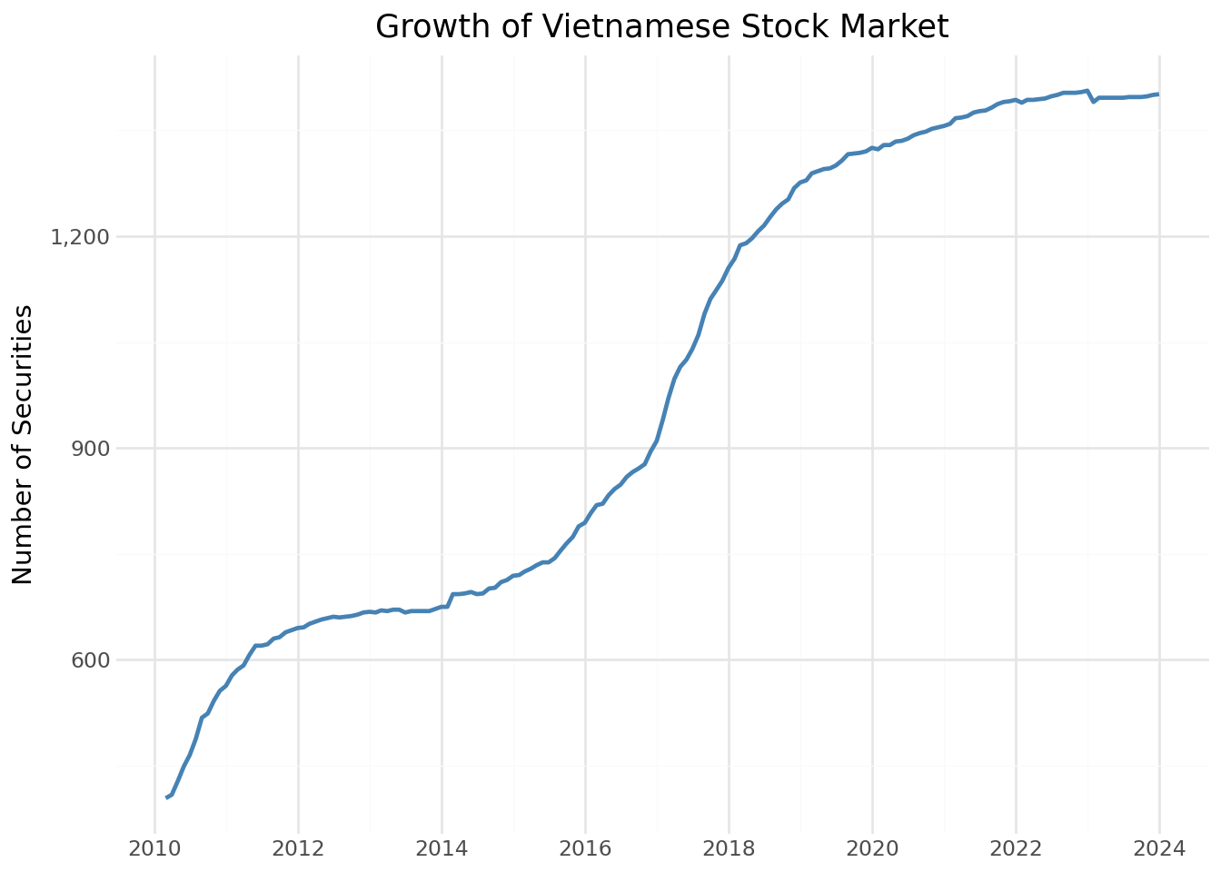
3.7.2 Market Capitalization Evolution
The aggregate market capitalization reflects the overall size and development of the Vietnamese equity market.
mktcap_figure = (
    ggplot(securities_over_time, aes(x="date", y="total_mktcap / 1000"))
    + geom_line(color="darkgreen", size=1)
    + labs(
        x="",
        y="Market Cap (Trillion VND)",
        title="Total Market Capitalization of Vietnamese Equities"
    )
    + scale_x_datetime(date_breaks="2 years", date_labels="%Y")
    + scale_y_continuous(labels=comma_format())
    + theme_minimal()
)
mktcap_figure.show()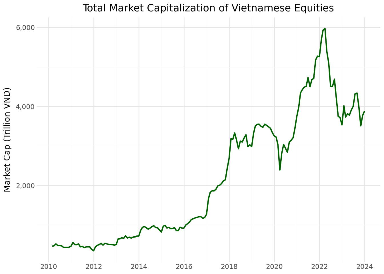
3.7.3 Return Distribution
Understanding the distribution of monthly returns helps identify potential data quality issues and characterize market risk.
return_distribution = (
    ggplot(prices_monthly, aes(x="ret_excess"))
    + geom_histogram(
        binwidth=0.02,
        fill="steelblue",
        color="white",
        alpha=0.7
    )
    + labs(
        x="Monthly Excess Return",
        y="Frequency",
        title="Distribution of Monthly Excess Returns"
    )
    + scale_x_continuous(limits=(-0.5, 0.5))
    + theme_minimal()
)
return_distribution.show()
/home/mikenguyen/project/tidyfinance/.venv/lib/python3.13/site-packages/plotnine/layer.py:293: PlotnineWarning: stat_bin : Removed 3264 rows containing non-finite values.
/home/mikenguyen/project/tidyfinance/.venv/lib/python3.13/site-packages/plotnine/layer.py:374: PlotnineWarning: geom_histogram : Removed 2 rows containing missing values.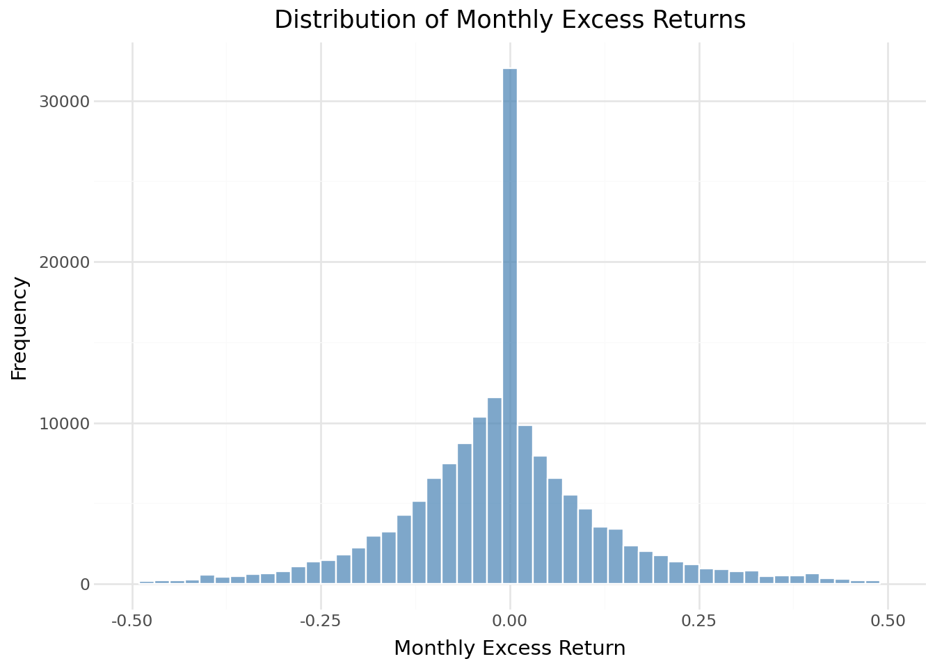
3.7.4 Coverage of Book Equity
Book equity is essential for constructing value portfolios. We examine what fraction of our sample has book equity data available over time.
# Merge prices with fundamentals
coverage_data = (prices_monthly
    .assign(year=lambda x: x["date"].dt.year)
    .groupby(["symbol", "year"])
    .tail(1)
    .merge(comp_vn[["symbol", "year", "be"]],
           on=["symbol", "year"],
           how="left")
)

# Compute coverage by year
be_coverage = (coverage_data
    .groupby("year")
    .apply(lambda x: pd.Series({
        "share_with_be": x["be"].notna().mean()
    }))
    .reset_index()
)

coverage_figure = (
    ggplot(be_coverage, aes(x="year", y="share_with_be"))
    + geom_line(color="darkorange", size=1)
    + geom_point(color="darkorange", size=2)
    + labs(
        x="Year",
        y="Share with Book Equity",
        title="Coverage of Book Equity Data"
    )
    + scale_y_continuous(labels=percent_format(), limits=(0, 1))
    + theme_minimal()
)
coverage_figure.show()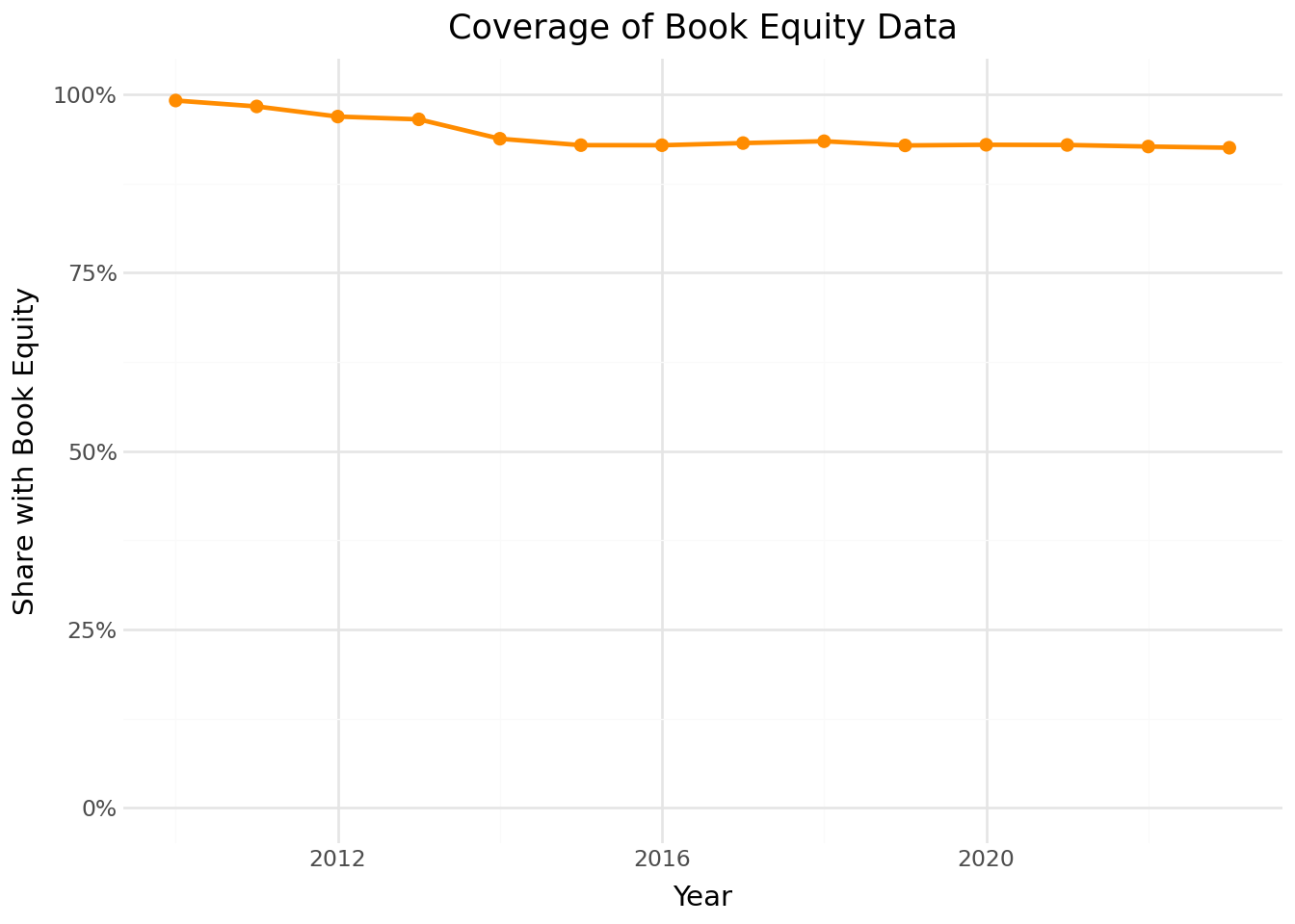
3.8 Merging Stock and Fundamental Data
The final step links price data with fundamental data using the stock symbol as the common identifier. This merged dataset forms the basis for constructing portfolios sorted on firm characteristics.
# Example: Create merged dataset for end-of-June each year
merged_data = (prices_monthly
.query("month == 6")
.merge(
comp_vn[["symbol", "year", "be", "op", "inv", "at"]],
on=["symbol", "year"],
how="left",
suffixes=("", "_fundamental")
)
)
# Convert BE from VND to BILLION VND
merged_data["be"] = merged_data["be"] / 1e9
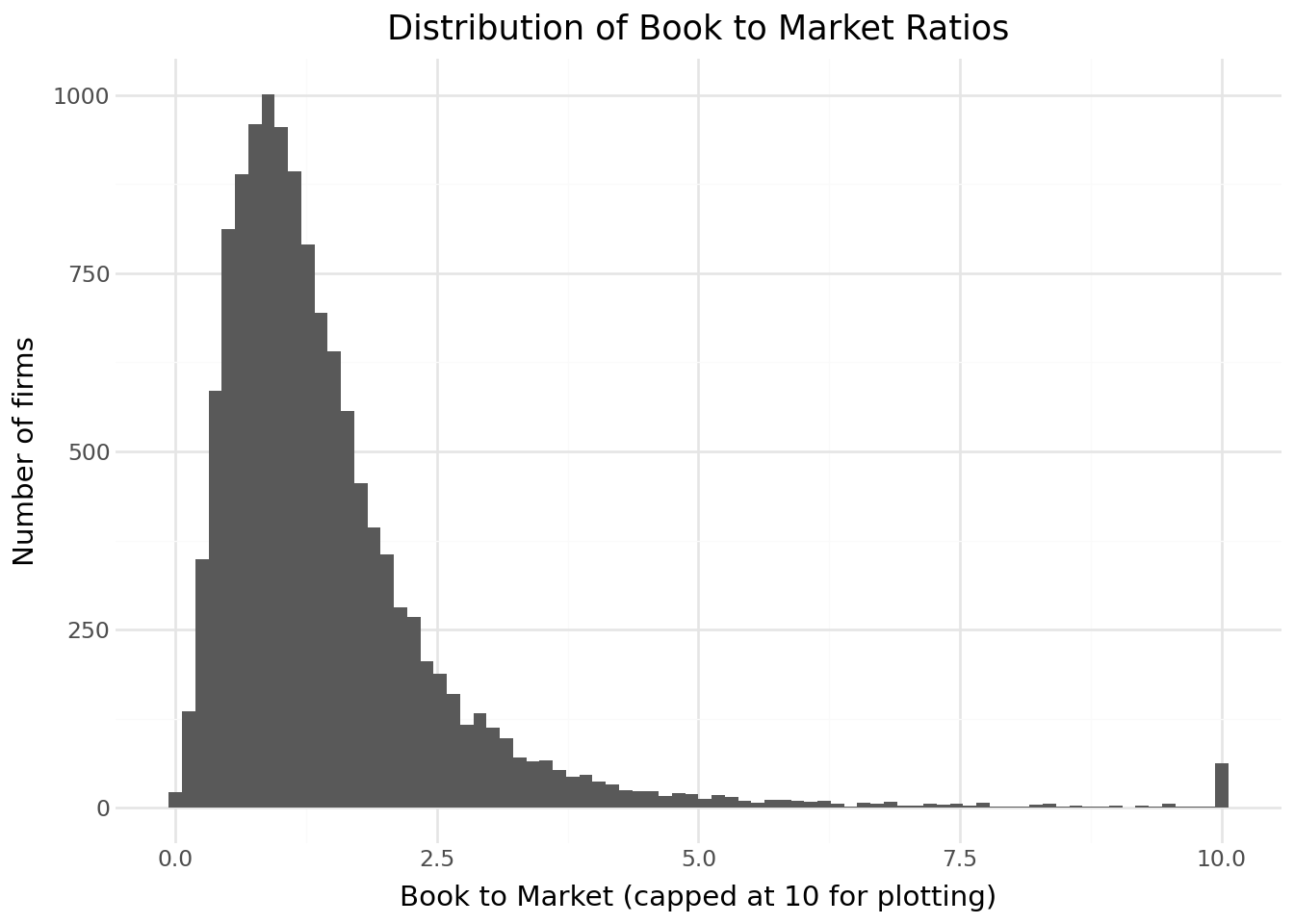
# Compute book-to-market ratio
merged_data["bm"] = merged_data["be"] / merged_data["mktcap"]
merged_data.loc[
(merged_data["bm"] <= 0) |
(merged_data["bm"] > 20),
"bm"
] = pd.NA
merged_data["bm"].describe(percentiles=[.01, .1, .5, .9, .99])
print(f"Merged observations: {len(merged_data):,}")
print(f"With book-to-market: {merged_data['bm'].notna().sum():,}")
merged_data.head(3)
merged_data.describe()
merged_dataMerged observations: 13,756
With book-to-market: 12,859| symbol | date | year | month | open | high | low | close | volume | adjusted_close | ... | mktcap | mktcap_lag | ret | risk_free | ret_excess | be | op | inv | at | bm | |
|---|---|---|---|---|---|---|---|---|---|---|---|---|---|---|---|---|---|---|---|---|---|
| 0 | A32 | 2019-06-30 | 2019.0 | 6.0 | 26.4 | 26.4 | 21.0 | 22.5 | 3700 | 35.929125 | ... | 153.000 | 179.52 | -0.170323 | 0.003333 | -0.173657 | 223.612748 | 0.232362 | -0.072329 | 4.349303e+11 | 1.461521 |
| 1 | A32 | 2020-06-30 | 2020.0 | 6.0 | 25.0 | 26.3 | 24.5 | 26.3 | 7500 | 38.811173 | ... | 178.840 | 187.00 | -0.067977 | 0.003333 | -0.071311 | 242.216943 | 0.195565 | 0.122698 | 4.882955e+11 | 1.354378 |
| 2 | A32 | 2021-06-30 | 2021.0 | 6.0 | 30.2 | 37.0 | 29.5 | 32.0 | 78400 | 45.363520 | ... | 217.600 | 214.20 | 0.015873 | 0.003333 | 0.012540 | 238.385190 | 0.157723 | 0.081581 | 5.281309e+11 | 1.095520 |
| 3 | A32 | 2022-06-30 | 2022.0 | 6.0 | 30.9 | 35.5 | 25.0 | 35.3 | 15200 | 47.503210 | ... | 240.040 | 210.12 | 0.142395 | 0.003333 | 0.139061 | 215.399735 | 0.172085 | 0.036584 | 5.474523e+11 | 0.897349 |
| 4 | A32 | 2023-06-30 | 2023.0 | 6.0 | 30.1 | 33.5 | 29.2 | 29.4 | 2400 | 35.064204 | ... | 199.920 | 204.68 | -0.023256 | 0.003333 | -0.026589 | 222.024135 | 0.174658 | -0.076752 | 5.054342e+11 | 1.110565 |
| ... | ... | ... | ... | ... | ... | ... | ... | ... | ... | ... | ... | ... | ... | ... | ... | ... | ... | ... | ... | ... | ... |
| 13751 | YTC | 2019-06-30 | 2019.0 | 6.0 | 70.0 | 79.9 | 70.0 | 79.9 | 38900 | 171.451817 | ... | 246.092 | 215.60 | 0.141429 | 0.003333 | 0.138095 | 59.901389 | 0.738190 | -0.021758 | 7.521980e+11 | 0.243411 |
| 13752 | YTC | 2020-06-30 | 2020.0 | 6.0 | 88.5 | 88.5 | 77.0 | 87.0 | 150640 | 180.966960 | ... | 267.960 | 272.58 | -0.016949 | 0.003333 | -0.020282 | 13.459082 | -0.458548 | 0.323501 | 9.955348e+11 | 0.050228 |
| 13753 | YTC | 2021-06-30 | 2021.0 | 6.0 | 76.0 | 115.5 | 61.0 | 61.0 | 34100 | 126.884880 | ... | 187.880 | 234.08 | -0.197368 | 0.003333 | -0.200702 | 21.746595 | 0.539521 | -0.215694 | 7.808035e+11 | 0.115747 |
| 13754 | YTC | 2022-06-30 | 2022.0 | 6.0 | 68.0 | 68.0 | 65.0 | 65.5 | 200 | 136.245240 | ... | 201.740 | 209.44 | -0.036765 | 0.003333 | -0.040098 | 32.403055 | 0.483088 | 0.182911 | 9.236206e+11 | 0.160618 |
| 13755 | YTC | 2023-06-30 | 2023.0 | 6.0 | 59.0 | 59.0 | 59.0 | 59.0 | 49545 | 122.724720 | ... | 181.720 | 181.72 | 0.000000 | 0.003333 | -0.003333 | 38.976624 | 0.450157 | 0.017930 | 9.401815e+11 | 0.214487 |
13756 rows × 21 columns
from plotnine import *
import numpy as np

bm_plot_data = (
    merged_data[["bm"]]
      .dropna()
      .assign(bm_plot=lambda x: x["bm"].clip(upper=10))
)

(
    ggplot(bm_plot_data, aes(x="bm_plot")) +
    geom_histogram(bins=80) +
    labs(
        title="Distribution of Book to Market Ratios",
        x="Book to Market (capped at 10 for plotting)",
        y="Number of firms"
    ) +
    theme_minimal()
)
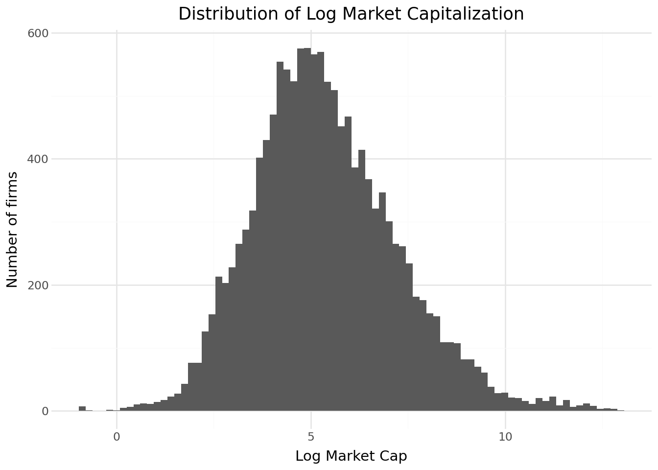
size_plot_data = (
    merged_data[["mktcap_lag"]]
      .dropna()
      .assign(log_size=lambda x: np.log(x["mktcap_lag"]))
)

(
    ggplot(size_plot_data, aes(x="log_size")) +
    geom_histogram(bins=80) +
    labs(
        title="Distribution of Log Market Capitalization",
        x="Log Market Cap",
        y="Number of firms"
    ) +
    theme_minimal()
)
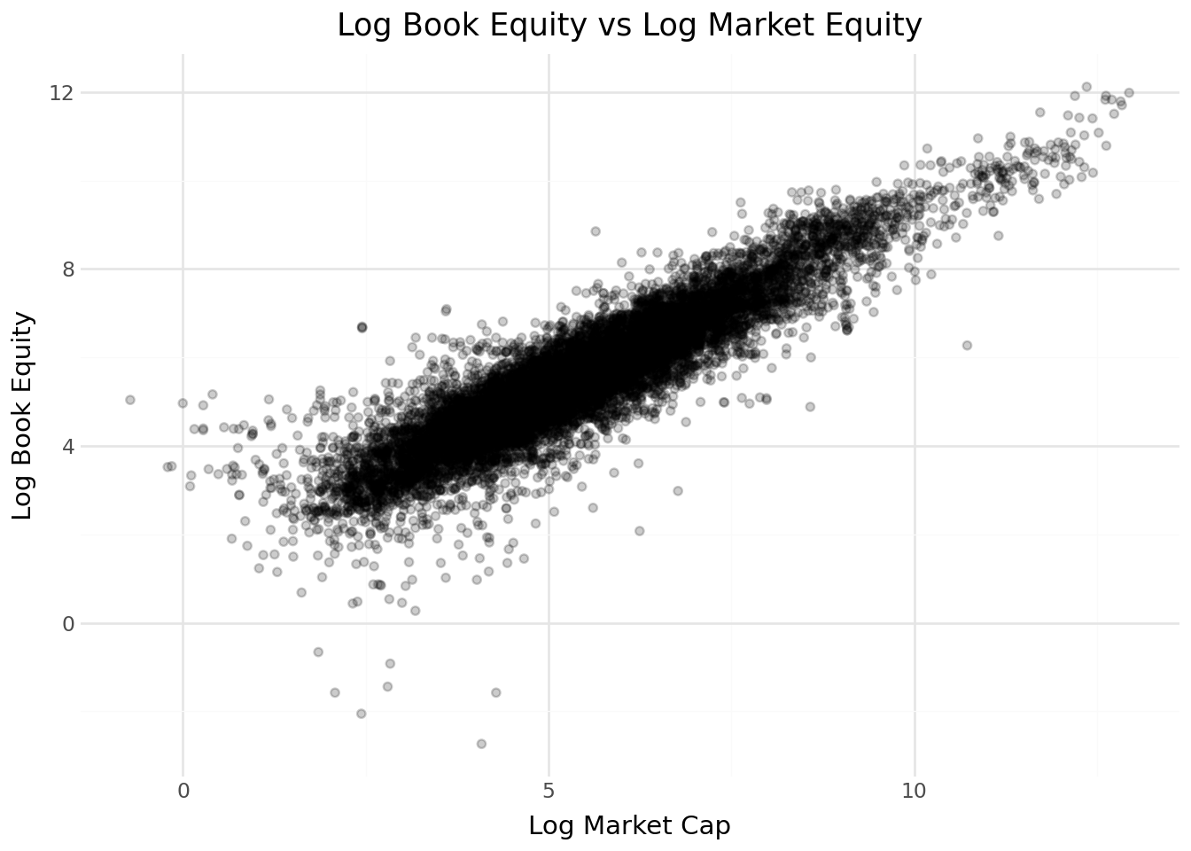
scatter_data = (
    merged_data[["be", "mktcap_lag"]]
      .dropna()
      .assign(
          log_be=lambda x: np.log(x["be"]),
          log_me=lambda x: np.log(x["mktcap_lag"])
      )
)

(
    ggplot(scatter_data, aes(x="log_me", y="log_be")) +
    geom_point(alpha=0.2) +
    labs(
        title="Log Book Equity vs Log Market Equity",
        x="Log Market Cap",
        y="Log Book Equity"
    ) +
    theme_minimal()
)
3.9 Key Takeaways
Datacore provides unified access to Vietnamese financial data through a modern cloud-based infrastructure, eliminating the need to aggregate data from multiple fragmented sources.
Company fundamentals from Datacore include comprehensive balance sheet, income statement, and cash flow data prepared according to Vietnamese Accounting Standards, which we map to standard variables used in international research.
Book equity computation follows the Fama-French methodology, accounting for deferred taxes and preferred stock to ensure comparability with US-based studies.
Stock price data includes adjustment factors for corporate actions, enabling accurate return calculations over long horizons.
Monthly frequency is standard for asset pricing research, reducing noise while maintaining sufficient observations for statistical inference.
Risk-free rate approximation uses Vietnamese government bond yields as a proxy, given the absence of a standardized short-term rate series comparable to US Treasury bills.
Data quality validation through descriptive statistics and visualization helps identify potential issues before conducting formal analyses.
Batch processing enables efficient handling of large daily datasets that would otherwise exceed memory constraints.