import pandas as pd
import numpy as np
import sqlite3
import statsmodels.formula.api as smf
from scipy.stats.mstats import winsorize

from plotnine import *
from mizani.formatters import percent_format, comma_format
from joblib import Parallel, delayed, cpu_count
from dateutil.relativedelta import relativedelta15 Beta Estimation
This chapter introduces one of the most fundamental concepts in financial economics: the exposure of an individual stock to systematic market risk. According to the Capital Asset Pricing Model (CAPM) developed by Sharpe (1964), Lintner (1965), and Mossin (1966), cross-sectional variation in expected asset returns should be determined by the covariance between an asset’s excess return and the excess return on the market portfolio. The regression coefficient that captures this relationship (commonly known as market beta) serves as the cornerstone of modern portfolio theory and remains widely used in practice for cost of capital estimation, performance attribution, and risk management.
In this chapter, we develop a complete framework for estimating market betas for Vietnamese stocks. We begin with a conceptual overview of the CAPM and its empirical implementation. We then demonstrate beta estimation using ordinary least squares regression, first for individual stocks and then scaled to the entire market using rolling-window estimation. To handle the computational demands of estimating betas for hundreds of stocks across many time periods, we introduce parallelization techniques that dramatically reduce processing time. Finally, we compare beta estimates derived from monthly versus daily returns and examine how betas vary across industries and over time in the Vietnamese market.
The chapter leverages several important computational concepts that extend beyond beta estimation itself. Rolling-window estimation is a technique applicable to any time-varying parameter, while parallelization provides a general solution for computationally intensive tasks that can be divided into independent subtasks.
15.1 Theoretical Foundation
15.1.1 The Capital Asset Pricing Model
The CAPM provides a theoretical framework linking expected returns to systematic risk. Under the model’s assumptions—including mean-variance optimizing investors, homogeneous expectations, and frictionless markets—the expected excess return on any asset \(i\) is proportional to its covariance with the market portfolio:
\[ E[r_i - r_f] = \beta_i \cdot E[r_m - r_f] \]
where \(r_i\) is the return on asset \(i\), \(r_f\) is the risk-free rate, \(r_m\) is the return on the market portfolio, and \(\beta_i\) is defined as:
\[ \beta_i = \frac{\text{Cov}(r_i, r_m)}{\text{Var}(r_m)} \]
The market beta \(\beta_i\) measures the sensitivity of asset \(i\)’s returns to market movements. A beta greater than one indicates the asset amplifies market movements, while a beta less than one indicates dampened sensitivity. A beta of zero would imply no systematic risk exposure, leaving only idiosyncratic risk that can be diversified away.
15.1.2 Empirical Implementation
In practice, we estimate beta by regressing excess stock returns on excess market returns:
\[ r_{i,t} - r_{f,t} = \alpha_i + \beta_i(r_{m,t} - r_{f,t}) + \varepsilon_{i,t} \tag{15.1}\]
where \(\alpha_i\) represents abnormal return (Jensen’s alpha), \(\beta_i\) is the market beta we seek to estimate, and \(\varepsilon_{i,t}\) is the idiosyncratic error term. Under the CAPM, \(\alpha_i\) should equal zero for all assets—any non-zero alpha represents a deviation from the model’s predictions.
Several practical considerations affect beta estimation:
Estimation Window: Longer windows provide more observations and thus more precise estimates, but may include outdated information if betas change over time. Common choices range from 36 to 60 months for monthly data.
Return Frequency: Monthly returns reduce noise but provide fewer observations. Daily returns offer more data points but may introduce microstructure effects and non-synchronous trading biases.
Market Proxy: The theoretical market portfolio includes all assets, but in practice we use a broad equity index. For Vietnam, we use the value-weighted market return constructed from our stock universe.
Minimum Observations: Requiring a minimum number of observations (e.g., 48 out of 60 months) helps avoid unreliable estimates from sparse data.
15.2 Setting Up the Environment
We begin by loading the necessary Python packages. The core packages handle data manipulation, statistical modeling, and database operations. We also import parallelization tools that will be essential when scaling our estimation to the full market.
We connect to our SQLite database containing the processed Vietnamese financial data from previous chapters.
tidy_finance = sqlite3.connect(database="data/tidy_finance_python.sqlite")15.3 Loading and Preparing Data
15.3.1 Stock Returns Data
We load the monthly stock returns data prepared in the Datacore chapter. The data includes excess returns (returns minus the risk-free rate) for all Vietnamese listed stocks.
prices_monthly = pd.read_sql_query(
    sql="""
        SELECT symbol, date, ret_excess
        FROM prices_monthly
    """,
    con=tidy_finance,
    parse_dates={"date"}
)

# Add year for merging with fundamentals
prices_monthly["year"] = prices_monthly["date"].dt.year

print(f"Loaded {len(prices_monthly):,} monthly observations")
print(f"Covering {prices_monthly['symbol'].nunique():,} unique stocks")
print(f"Date range: {prices_monthly['date'].min():%Y-%m} to {prices_monthly['date'].max():%Y-%m}")
Loaded 209,495 monthly observations
Covering 1,837 unique stocks
Date range: 2010-01 to 2025-05prices_daily = pd.read_sql_query(
sql="""
SELECT symbol, date, ret_excess
FROM prices_daily
""",
con=tidy_finance,
parse_dates={"date"}
)15.3.2 Company Information
We load company information to enable industry-level analysis of beta estimates.
comp_vn = pd.read_sql_query(
    sql="""
        SELECT symbol, datadate, icb_name_vi
        FROM comp_vn
    """,
    con=tidy_finance,
    parse_dates={"datadate"}
)

# Extract year for merging
comp_vn["year"] = comp_vn["datadate"].dt.year

print(f"Company data: {comp_vn['symbol'].nunique():,} firms")
Company data: 1,502 firms15.3.3 Market Excess Returns
For the market portfolio proxy, we use the value-weighted market excess return. If you have constructed Fama-French factors in a previous chapter, load them here. Otherwise, we can construct a simple market return from our stock data.
# Option 1: Load pre-computed market factor
factors_ff3_monthly = pd.read_sql_query(
    sql="SELECT date, mkt_excess FROM factors_ff3_monthly",
    con=tidy_finance,
    parse_dates={"date"}
)

# Option 2: Construct market return from stock data (if factors not available)
# This computes the value-weighted average return across all stocks
def compute_market_return(prices_df):
    """
    Compute value-weighted market return from individual stock returns.

    Parameters
    ----------
    prices_df : pd.DataFrame
        Stock returns with mktcap_lag for weighting

    Returns
    -------
    pd.DataFrame
        Monthly market excess returns
    """
    market_return = (prices_df
        .groupby("date")
        .apply(lambda x: np.average(x["ret_excess"], weights=x["mktcap_lag"]))
        .reset_index(name="mkt_excess")
    )
    return market_return
15.3.4 Merging Datasets
We combine the stock returns with market returns and company information to create our estimation dataset.
# Merge stock returns with market returns
prices_monthly = prices_monthly.merge(
    factors_ff3_monthly,
    on="date",
    how="left"
)

# Merge with company information for industry classification
prices_monthly = prices_monthly.merge(
    comp_vn[["symbol", "year", "icb_name_vi"]],
    on=["symbol", "year"],
    how="left"
)

# Remove observations with missing data
prices_monthly = prices_monthly.dropna(subset=["ret_excess", "mkt_excess"])

print(f"Final estimation sample: {len(prices_monthly):,} observations")
Final estimation sample: 169,983 observations15.3.5 Handling Outliers
Extreme returns can unduly influence regression estimates. We apply winsorization to limit the impact of outliers while preserving the general distribution of returns. Winsorization at the 1% level replaces values below the 1st percentile with the 1st percentile value, and values above the 99th percentile with the 99th percentile value.
def winsorize_returns(df, columns, limits=(0.01, 0.01)):
    """
    Apply winsorization to return columns to limit outlier influence.

    Parameters
    ----------
    df : pd.DataFrame
        DataFrame containing return columns
    columns : list
        Column names to winsorize
    limits : tuple
        Lower and upper percentile limits for winsorization

    Returns
    -------
    pd.DataFrame
        DataFrame with winsorized columns
    """
    df = df.copy()
    for col in columns:
        df[col] = winsorize(df[col], limits=limits)
    return df

prices_monthly = winsorize_returns(
    prices_monthly,
    columns=["ret_excess", "mkt_excess"],
    limits=(0.01, 0.01)
)

print("Return distributions after winsorization:")
print(prices_monthly[["ret_excess", "mkt_excess"]].describe().round(4))
Return distributions after winsorization:
ret_excess mkt_excess
count 169983.0000 169983.0000
mean 0.0011 -0.0102
std 0.1548 0.0579
min -0.4078 -0.1794
25% -0.0700 -0.0384
50% -0.0033 -0.0084
75% 0.0531 0.0219
max 0.6117 0.122115.4 Estimating Beta for Individual Stocks
15.4.1 Single Stock Example
Before scaling to the full market, we demonstrate beta estimation for a single well-known Vietnamese stock. We use Vingroup (VIC), one of the largest conglomerates in Vietnam with significant exposure to real estate, retail, and automotive sectors.
# Filter data for Vingroup
vic_data = prices_monthly.query("symbol == 'VIC'").copy()

print(f"VIC observations: {len(vic_data)}")
print(f"Date range: {vic_data['date'].min():%Y-%m} to {vic_data['date'].max():%Y-%m}")
VIC observations: 150
Date range: 2011-07 to 2023-12We estimate the CAPM regression using ordinary least squares via the statsmodels package. The formula interface provides a convenient way to specify regression models.
# Estimate CAPM for Vingroup
model_vic = smf.ols(
    formula="ret_excess ~ mkt_excess",
    data=vic_data
).fit()

# Display regression results
print(model_vic.summary())
OLS Regression Results
==============================================================================
Dep. Variable: ret_excess R-squared: 0.153
Model: OLS Adj. R-squared: 0.147
Method: Least Squares F-statistic: 26.67
Date: Sat, 14 Feb 2026 Prob (F-statistic): 7.66e-07
Time: 07:51:19 Log-Likelihood: 131.96
No. Observations: 150 AIC: -259.9
Df Residuals: 148 BIC: -253.9
Df Model: 1
Covariance Type: nonrobust
==============================================================================
coef std err t P>|t| [0.025 0.975]
------------------------------------------------------------------------------
Intercept -0.0075 0.008 -0.895 0.372 -0.024 0.009
mkt_excess 0.7503 0.145 5.164 0.000 0.463 1.037
==============================================================================
Omnibus: 39.111 Durbin-Watson: 2.039
Prob(Omnibus): 0.000 Jarque-Bera (JB): 107.620
Skew: -1.015 Prob(JB): 4.27e-24
Kurtosis: 6.619 Cond. No. 17.6
==============================================================================
Notes:
[1] Standard Errors assume that the covariance matrix of the errors is correctly specified.The regression output provides several important pieces of information:
- Beta (mkt_excess coefficient): The estimated market sensitivity. A beta above 1 indicates VIC amplifies market movements.
- Alpha (Intercept): The abnormal return not explained by market exposure. Under CAPM, this should be zero.
- R-squared: The proportion of return variation explained by market movements.
- t-statistics: Test whether coefficients differ significantly from zero.
# Extract key estimates
coefficients = model_vic.summary2().tables[1]

print("\nKey estimates for Vingroup (VIC):")
print(f"  Beta:  {coefficients.loc['mkt_excess', 'Coef.']:.3f}")
print(f"  Alpha: {coefficients.loc['Intercept', 'Coef.']:.4f}")
print(f"  R²:    {model_vic.rsquared:.3f}")
Key estimates for Vingroup (VIC):
  Beta:  0.750
  Alpha: -0.0075
  R²:    0.153
15.4.2 CAPM Estimation Function
We create a reusable function that estimates the CAPM and returns results in a standardized format. The function includes a minimum observations requirement to avoid unreliable estimates from sparse data.
def estimate_capm(data, min_obs=48):
    """
    Estimate CAPM regression and return coefficients.

    This function regresses excess stock returns on excess market returns
    and extracts the coefficient estimates along with t-statistics.

    Parameters
    ----------
    data : pd.DataFrame
        DataFrame with 'ret_excess' and 'mkt_excess' columns
    min_obs : int
        Minimum number of observations required for estimation

    Returns
    -------
    pd.DataFrame
        DataFrame with coefficient estimates and t-statistics,
        or empty DataFrame if insufficient observations
    """
    if len(data) < min_obs:
        return pd.DataFrame()

    try:
        # Estimate OLS regression
        model = smf.ols(
            formula="ret_excess ~ mkt_excess",
            data=data
        ).fit()

        # Extract coefficient table
        coef_table = model.summary2().tables[1]

        # Format results
        results = pd.DataFrame({
            "coefficient": ["alpha", "beta"],
            "estimate": [
                coef_table.loc["Intercept", "Coef."],
                coef_table.loc["mkt_excess", "Coef."]
            ],
            "t_statistic": [
                coef_table.loc["Intercept", "t"],
                coef_table.loc["mkt_excess", "t"]
            ],
            "r_squared": model.rsquared
        })

        return results

    except Exception as e:
        # Return empty DataFrame if estimation fails
        return pd.DataFrame()
15.5 Rolling-Window Estimation
15.5.1 Motivation for Rolling Windows
Stock betas are not constant over time. A company’s business mix, leverage, and operating environment evolve, causing its systematic risk exposure to change. To capture this time variation, we use rolling-window estimation: at each point in time, we estimate beta using only data from a fixed lookback period (e.g., the past 60 months).
Rolling-window estimation involves a trade-off:
- Longer windows provide more observations and thus more precise estimates, but may include stale information.
- Shorter windows are more responsive to changes but produce noisier estimates.
A common choice in academic research is 60 months (5 years) of monthly data, requiring at least 48 valid observations for estimation.
15.5.2 Rolling Window Implementation
The following function implements rolling-window CAPM estimation. For each month in the sample, it looks back over the specified window and estimates beta using all available data within that window.
def roll_capm_estimation(data, look_back=60, min_obs=48):
    """
    Perform rolling-window CAPM estimation.

    This function slides a window across time, estimating the CAPM
    regression at each point using the most recent 'look_back' months
    of data.

    Parameters
    ----------
    data : pd.DataFrame
        DataFrame with 'date', 'ret_excess', and 'mkt_excess' columns
    look_back : int
        Number of months in the estimation window
    min_obs : int
        Minimum observations required within each window

    Returns
    -------
    pd.DataFrame
        Time series of coefficient estimates with dates
    """
    # Ensure data is sorted by date
    data = data.sort_values("date").copy()

    # Get unique dates
    dates = data["date"].drop_duplicates().sort_values()

    # Container for results
    results = []

    # Slide window across dates
    for i in range(look_back - 1, len(dates)):
        # Define window boundaries
        end_date = dates.iloc[i]
        start_date = end_date - relativedelta(months=look_back - 1)

        # Extract data within window
        window_data = data.query("date >= @start_date and date <= @end_date")

        # Estimate CAPM for this window
        window_results = estimate_capm(window_data, min_obs=min_obs)

        if not window_results.empty:
            window_results["date"] = end_date
            results.append(window_results)

    # Combine all results
    if results:
        return pd.concat(results, ignore_index=True)
    else:
        return pd.DataFrame()
15.5.3 Example: Rolling Betas for Selected Stocks
We demonstrate rolling-window estimation for several well-known Vietnamese stocks spanning different industries.
# Define example stocks
examples = pd.DataFrame({
    "symbol": ["FPT", "VNM", "VIC", "HPG", "VCB"],
    "company": [
        "FPT Corporation",      # Technology
        "Vinamilk",             # Consumer goods
        "Vingroup",             # Real estate/conglomerate
        "Hoa Phat Group",       # Steel/materials
        "Vietcombank"           # Banking
    ]
})

# Check data availability for each example
data_availability = (prices_monthly
    .query("symbol in @examples['symbol']")
    .groupby("symbol")
    .agg(
        n_obs=("date", "count"),
        first_date=("date", "min"),
        last_date=("date", "max")
    )
    .reset_index()
)

print("Data availability for example stocks:")
print(data_availability)
Data availability for example stocks:
symbol n_obs first_date last_date
0 FPT 150 2011-07-31 2023-12-31
1 HPG 150 2011-07-31 2023-12-31
2 VCB 150 2011-07-31 2023-12-31
3 VIC 150 2011-07-31 2023-12-31
4 VNM 150 2011-07-31 2023-12-31# Estimate rolling betas for example stocks
example_data = prices_monthly.query("symbol in @examples['symbol']")
capm_examples = (example_data
.groupby("symbol", group_keys=True)
.apply(lambda x: roll_capm_estimation(x), include_groups=False)
.reset_index()
.drop(columns="level_1", errors="ignore")
)
# Filter to beta estimates only
beta_examples = (capm_examples
.query("coefficient == 'beta'")
.merge(examples, on="symbol")
)
print(f"Rolling beta estimates: {len(beta_examples):,} observations")Rolling beta estimates: 455 observations15.5.4 Visualizing Rolling Betas
Figure 22.6 displays the time series of beta estimates for our example stocks. The figure reveals how systematic risk exposure evolves differently across industries.
rolling_beta_figure = (
    ggplot(
        beta_examples,
        aes(x="date", y="estimate", color="company")
    )
    + geom_line(size=0.8)
    + geom_hline(yintercept=1, linetype="dashed", color="gray", alpha=0.7)
    + labs(
        x="",
        y="Beta",
        color="",
        title="Rolling Beta Estimates (60-Month Window)"
    )
    + scale_x_datetime(date_breaks="2 years", date_labels="%Y")
    + theme_minimal()
    + theme(legend_position="bottom")
)
rolling_beta_figure.show()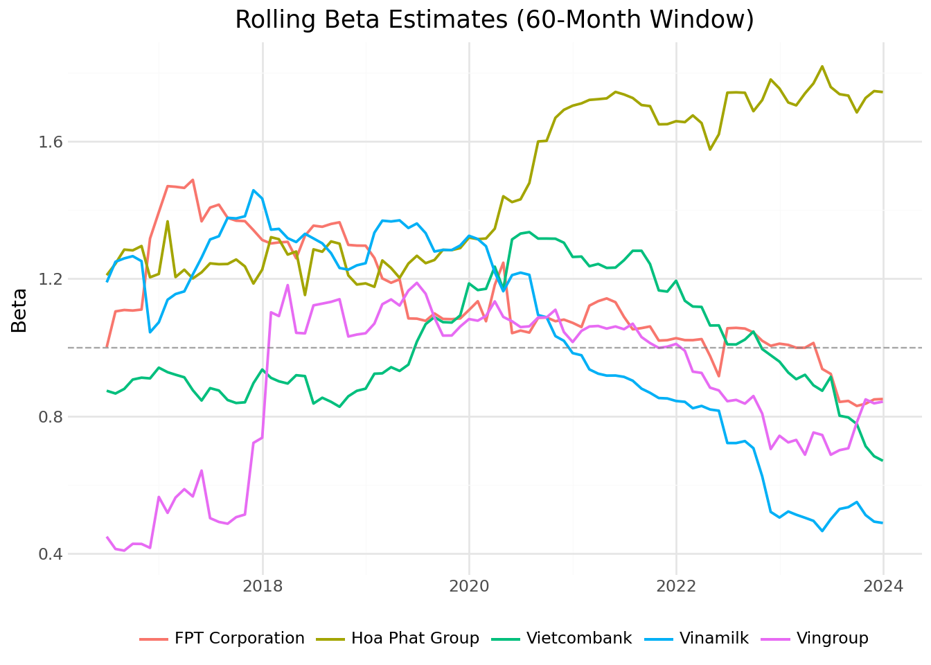
Several patterns emerge from the figure:
Industry differences: Technology and banking stocks may exhibit different beta patterns than real estate or consumer goods companies.
Time variation: Betas are not constant. They respond to changes in business conditions, leverage, and market regimes.
Crisis periods: Market stress periods (e.g., 2008 financial crisis, 2020 COVID-19) often see beta estimates change as correlations across stocks increase.
15.6 Parallelized Estimation for the Full Market
15.6.1 The Computational Challenge
Estimating rolling betas for all stocks in our database is computationally intensive. With hundreds of stocks, each requiring rolling estimation across many time periods, sequential processing would take considerable time. Fortunately, beta estimation for different stocks is independent (i.e., the estimate for stock A does not depend on the estimate for stock B). This independence makes the problem ideal for parallelization.
15.6.2 Setting Up Parallel Processing
We use the joblib library to distribute computation across multiple CPU cores. The Parallel class manages worker processes, while delayed wraps function calls for deferred execution.
# Determine available cores (reserve one for system operations)
n_cores = max(1, cpu_count() - 1)
print(f"Available cores for parallel processing: {n_cores}")
Available cores for parallel processing: 315.6.3 Parallel Beta Estimation
The following code estimates rolling betas for all stocks in parallel. Each stock is processed independently by a separate worker.
def estimate_all_betas_parallel(data, n_cores, look_back=60, min_obs=48):
    """
    Estimate rolling betas for all stocks using parallel processing.

    Parameters
    ----------
    data : pd.DataFrame
        Full dataset with all stocks
    n_cores : int
        Number of CPU cores to use
    look_back : int
        Months in estimation window
    min_obs : int
        Minimum observations required

    Returns
    -------
    pd.DataFrame
        Beta estimates for all stocks and dates
    """
    # Group data by stock
    grouped = data.groupby("symbol", group_keys=False)

    # Define worker function
    def process_stock(name, group):
        result = roll_capm_estimation(group, look_back=look_back, min_obs=min_obs)
        if not result.empty:
            result["symbol"] = name
        return result

    # Execute in parallel
    results = Parallel(n_jobs=n_cores, verbose=1)(
        delayed(process_stock)(name, group)
        for name, group in grouped
    )

    # Combine results
    results = [r for r in results if not r.empty]
    if results:
        return pd.concat(results, ignore_index=True)
    else:
        return pd.DataFrame()
# Estimate betas for all stocks
print("Estimating rolling betas for all stocks...")
capm_monthly = estimate_all_betas_parallel(
prices_monthly,
n_cores=n_cores,
look_back=60,
min_obs=48
)
print(f"\nCompleted: {len(capm_monthly):,} coefficient estimates")
print(f"Unique stocks: {capm_monthly['symbol'].nunique():,}")15.6.4 Storing Results
We save the CAPM estimates to our database for use in subsequent chapters.
capm_monthly.to_sql(
    name="capm_monthly",
    con=tidy_finance,
    if_exists="replace",
    index=False
)

print("CAPM estimates saved to database.")
For subsequent analysis, we load the pre-computed estimates:
capm_monthly = pd.read_sql_query(
    sql="SELECT * FROM capm_monthly",
    con=tidy_finance,
    parse_dates={"date"}
)

print(f"Loaded {len(capm_monthly):,} CAPM estimates")
Loaded 161,580 CAPM estimates15.7 Beta Estimation Using Daily Returns
While monthly returns are standard in academic research, some applications benefit from higher-frequency data:
- Shorter estimation windows: Daily data allows meaningful estimation over shorter periods (e.g., 3 months rather than 5 years).
- More responsive estimates: Daily betas capture changes more quickly.
- Event studies: High-frequency betas are useful for analyzing market reactions to specific events.
However, daily data introduces additional challenges:
- Microstructure noise: Bid-ask bounce and other trading frictions add noise to returns.
- Non-synchronous trading: Less liquid stocks may not trade every day, biasing beta estimates downward.
- Computational burden: Daily data is roughly 21 times larger than monthly data.
15.7.1 Batch Processing for Daily Data
Given the size of daily data, we process stocks in batches to manage memory constraints. This approach loads and processes a subset of stocks, saves results, and proceeds to the next batch.
def compute_market_return_daily(tidy_finance):
    """
    Compute daily value-weighted market excess return from stock data.
    """
    # Load daily prices with market cap for weighting
    prices_daily_full = pd.read_sql_query(
        sql="""
            SELECT p.symbol, p.date, p.ret_excess, m.mktcap_lag
            FROM prices_daily p
            LEFT JOIN prices_monthly m ON p.symbol = m.symbol
                AND strftime('%Y-%m', p.date) = strftime('%Y-%m', m.date)
        """,
        con=tidy_finance,
        parse_dates={"date"}
    )

    # Compute value-weighted market return each day
    mkt_daily = (prices_daily_full
        .dropna(subset=["ret_excess", "mktcap_lag"])
        .groupby("date")
        .apply(lambda x: np.average(x["ret_excess"], weights=x["mktcap_lag"]))
        .reset_index(name="mkt_excess")
    )

    return mkt_daily


def roll_capm_estimation_daily(data, look_back_days=1260, min_obs=1000):
    """
    Perform rolling-window CAPM estimation using daily data.

    Parameters
    ----------
    data : pd.DataFrame
        DataFrame with 'date', 'ret_excess', and 'mkt_excess' columns
    look_back_days : int
        Number of trading days in the estimation window
    min_obs : int
        Minimum daily observations required within each window

    Returns
    -------
    pd.DataFrame
        Time series of coefficient estimates with dates
    """
    data = data.sort_values("date").copy()
    dates = data["date"].drop_duplicates().sort_values().reset_index(drop=True)

    results = []

    for i in range(look_back_days - 1, len(dates)):
        end_date = dates.iloc[i]
        start_idx = max(0, i - look_back_days + 1)
        start_date = dates.iloc[start_idx]

        window_data = data.query("date >= @start_date and date <= @end_date")
        window_results = estimate_capm(window_data, min_obs=min_obs)

        if not window_results.empty:
            window_results["date"] = end_date
            results.append(window_results)

    if results:
        return pd.concat(results, ignore_index=True)
    else:
        return pd.DataFrame()


def estimate_daily_betas_batch(symbols, tidy_finance, n_cores, batch_size=500,
                                look_back_days=1260, min_obs=1000):
    """
    Estimate rolling betas from daily data using batch processing.
    """
    # First, compute or load market return
    print("Computing daily market excess returns...")
    mkt_daily = compute_market_return_daily(tidy_finance)
    print(f"Market returns: {len(mkt_daily)} days")

    n_batches = int(np.ceil(len(symbols) / batch_size))
    all_results = []

    for j in range(n_batches):
        batch_start = j * batch_size
        batch_end = min((j + 1) * batch_size, len(symbols))
        batch_symbols = symbols[batch_start:batch_end]

        symbol_list = ", ".join(f"'{s}'" for s in batch_symbols)

        query = f"""
            SELECT symbol, date, ret_excess
            FROM prices_daily
            WHERE symbol IN ({symbol_list})
        """

        prices_daily_batch = pd.read_sql_query(
            sql=query,
            con=tidy_finance,
            parse_dates={"date"}
        )

        # Merge with market excess return
        prices_daily_batch = prices_daily_batch.merge(
            mkt_daily,
            on="date",
            how="inner"
        )

        # Group by symbol and estimate betas
        grouped = prices_daily_batch.groupby("symbol", group_keys=False)

        # Parallel estimation
        batch_results = Parallel(n_jobs=n_cores)(
            delayed(lambda name, group:
                roll_capm_estimation_daily(group, look_back_days=look_back_days, min_obs=min_obs)
                .assign(symbol=name)
            )(name, group)
            for name, group in grouped
        )

        batch_results = [r for r in batch_results if r is not None and not r.empty]

        if batch_results:
            all_results.append(pd.concat(batch_results, ignore_index=True))

        print(f"Batch {j+1}/{n_batches} complete")

    if all_results:
        return pd.concat(all_results, ignore_index=True)
    else:
        return pd.DataFrame()
symbols = prices_monthly["symbol"].unique().tolist()
capm_daily = estimate_daily_betas_batch(
symbols=symbols,
tidy_finance=tidy_finance,
n_cores=n_cores,
batch_size=500,
look_back_days=1260, # ~5 years of trading days
min_obs=1000
)
print(f"Daily beta estimates: {len(capm_daily):,}")capm_daily.to_sql(
name="capm_daily",
con=tidy_finance,
if_exists="replace",
index=False
)
print("CAPM estimates saved to database.")For subsequent analysis, we load the pre-computed estimates:
capm_daily = pd.read_sql_query(
    sql="SELECT * FROM capm_daily",
    con=tidy_finance,
    parse_dates={"date"}
)

print(f"Loaded {len(capm_daily):,} CAPM estimates")
Loaded 3,394,490 CAPM estimates15.8 Analyzing Beta Estimates
15.8.1 Extracting Beta Estimates
We extract the beta coefficient estimates from our CAPM results for analysis.
# Extract monthly betas
beta_monthly = (capm_monthly
    .query("coefficient == 'beta'")
    .rename(columns={"estimate": "beta"})
    [["symbol", "date", "beta"]]
    .assign(frequency="monthly")
)

# Save to database
beta_monthly.to_sql(
    name="beta_monthly",
    con=tidy_finance,
    if_exists="replace",
    index=False
)

print(f"Monthly betas: {len(beta_monthly):,} observations")
print(f"Unique stocks: {beta_monthly['symbol'].nunique():,}")
Monthly betas: 80,790 observations
Unique stocks: 1,383# Load pre-computed betas
beta_monthly = pd.read_sql_query(
sql="SELECT * FROM beta_monthly",
con=tidy_finance,
parse_dates={"date"}
)15.8.2 Summary Statistics
We examine the distribution of beta estimates to verify their reasonableness.
print("Beta Summary Statistics:")
print(beta_monthly["beta"].describe().round(3))

# Additional diagnostics
print(f"\nStocks with negative average beta: {(beta_monthly.groupby('symbol')['beta'].mean() < 0).sum()}")
print(f"Stocks with beta > 2: {(beta_monthly.groupby('symbol')['beta'].mean() > 2).sum()}")
Beta Summary Statistics:
count 80790.000
mean 0.501
std 0.539
min -1.345
25% 0.130
50% 0.447
75% 0.832
max 2.678
Name: beta, dtype: float64
Stocks with negative average beta: 177
Stocks with beta > 2: 515.8.3 Beta Distribution Across Industries
Different industries have different exposures to systematic market risk based on their business models, operating leverage, and financial leverage. Figure 15.2 shows the distribution of firm-level average betas across Vietnamese industries.
# Merge betas with industry information
beta_with_industry = (beta_monthly
    .merge(
        prices_monthly[["symbol", "date", "icb_name_vi"]].drop_duplicates(),
        on=["symbol", "date"],
        how="left"
    )
    .dropna(subset=["icb_name_vi"])
)

# Compute firm-level average beta by industry
beta_by_industry = (beta_with_industry
    .groupby(["icb_name_vi", "symbol"])["beta"]
    .mean()
    .reset_index()
)

# Order industries by median beta
industry_order = (beta_by_industry
    .groupby("icb_name_vi")["beta"]
    .median()
    .sort_values()
    .index.tolist()
)

# Select top 10 industries by number of firms for clearer visualization
top_industries = (beta_by_industry
    .groupby("icb_name_vi")
    .size()
    .nlargest(10)
    .index.tolist()
)

beta_by_industry_filtered = beta_by_industry.query("icb_name_vi in @top_industries")
beta_industry_figure = (
ggplot(
beta_by_industry_filtered,
aes(x="icb_name_vi", y="beta")
)
+ geom_boxplot(fill="steelblue", alpha=0.7)
+ geom_hline(yintercept=1, linetype="dashed", color="red", alpha=0.7)
+ coord_flip()
+ labs(
x="",
y="Beta",
title="Beta Distribution by Industry"
)
+ theme_minimal()
)
beta_industry_figure.show()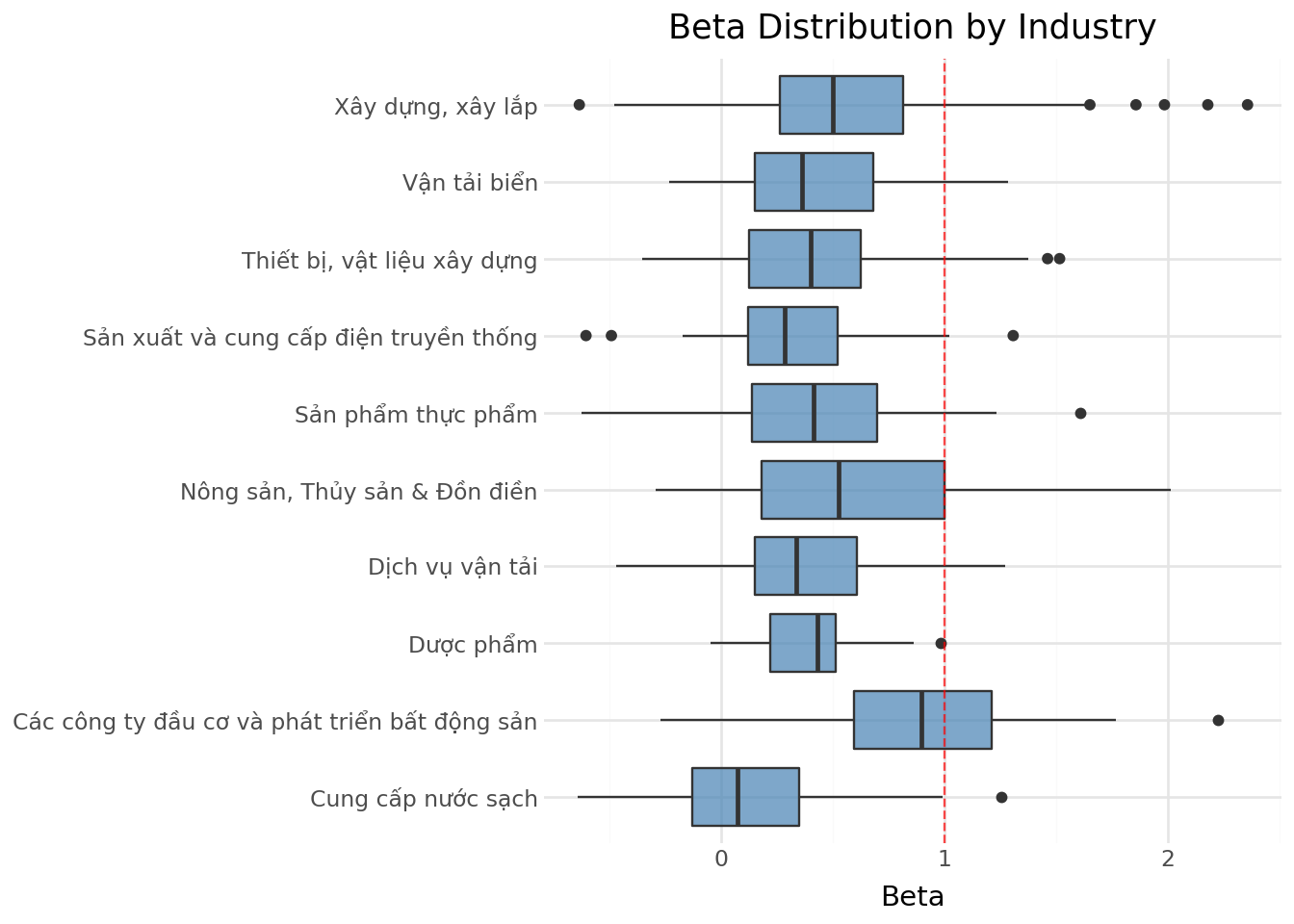
15.8.4 Time Variation in Cross-Sectional Beta Distribution
Betas vary not only across stocks but also over time. Figure 15.3 shows how the cross-sectional distribution of betas has evolved in the Vietnamese market.
# Compute monthly quantiles
beta_quantiles = (beta_monthly
    .groupby("date")["beta"]
    .quantile(q=np.arange(0.1, 1.0, 0.1))
    .reset_index()
    .rename(columns={"level_1": "quantile"})
    .assign(quantile=lambda x: (x["quantile"] * 100).astype(int).astype(str) + "%")
)

beta_quantiles_figure = (
    ggplot(
        beta_quantiles,
        aes(x="date", y="beta", color="quantile")
    )
    + geom_line(alpha=0.8)
    + geom_hline(yintercept=1, linetype="dashed", color="gray")
    + labs(
        x="",
        y="Beta",
        color="Quantile",
        title="Cross-Sectional Distribution of Betas Over Time"
    )
    + scale_x_datetime(date_breaks="2 years", date_labels="%Y")
    + theme_minimal()
)
beta_quantiles_figure.show()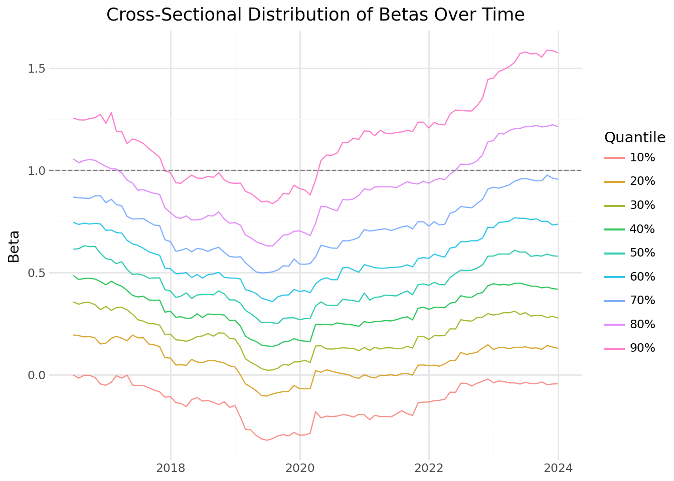
The figure reveals several interesting patterns:
Level shifts: The entire distribution of betas can shift over time, reflecting changes in market-wide correlation.
Dispersion changes: During market stress, the spread between high and low beta stocks may change as correlations move.
Trends: Some periods show trending behavior in betas, possibly reflecting structural changes in the economy.
15.8.5 Coverage Analysis
We verify that our estimation procedure produces reasonable coverage across the sample. Figure 15.4 shows the fraction of stocks with available beta estimates over time.
# Count stocks with and without betas
coverage = (prices_monthly
    .groupby("date")["symbol"]
    .nunique()
    .reset_index(name="total_stocks")
    .merge(
        beta_monthly.groupby("date")["symbol"].nunique().reset_index(name="with_beta"),
        on="date",
        how="left"
    )
    .fillna(0)
    .assign(coverage=lambda x: x["with_beta"] / x["total_stocks"])
)

coverage_figure = (
    ggplot(coverage, aes(x="date", y="coverage"))
    + geom_line(color="steelblue", size=1)
    + labs(
        x="",
        y="Share with Beta Estimate",
        title="Beta Estimation Coverage Over Time"
    )
    + scale_y_continuous(labels=percent_format(), limits=(0, 1))
    + scale_x_datetime(date_breaks="2 years", date_labels="%Y")
    + theme_minimal()
)
coverage_figure.show()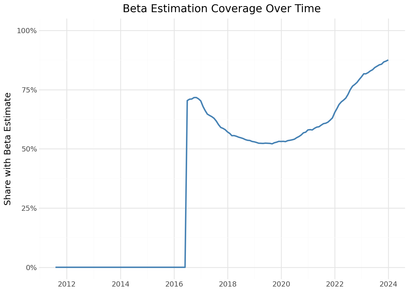
Coverage is lower in early years because stocks need sufficient return history (at least 48 months) before their betas can be estimated. As the market matures and stocks accumulate longer histories, coverage approaches 100%.
15.9 Comparing Monthly and Daily Beta Estimates
When both monthly and daily beta estimates are available, we can compare them to understand how estimation frequency affects results.
# Combine monthly and daily estimates
beta_daily = (capm_daily
    .query("coefficient == 'beta'")
    .rename(columns={"estimate": "beta"})
    [["symbol", "date", "beta"]]
    .assign(frequency="daily")
)

beta_combined = pd.concat([beta_monthly, beta_daily], ignore_index=True)
# Filter to example stocks
beta_comparison = (beta_combined
.merge(examples, on="symbol")
.query("symbol in ['VIC', 'FPT']") # Select two for clarity
)
comparison_figure = (
ggplot(
beta_comparison,
aes(x="date", y="beta", color="frequency", linetype="frequency")
)
+ geom_line(size=0.8)
+ facet_wrap("~company", ncol=1)
+ labs(
x="",
y="Beta",
color="Data Frequency",
linetype="Data Frequency",
title="Monthly vs Daily Beta Estimates"
)
+ scale_x_datetime(date_breaks="2 years", date_labels="%Y")
+ theme_minimal()
+ theme(legend_position="bottom")
)
comparison_figure.show()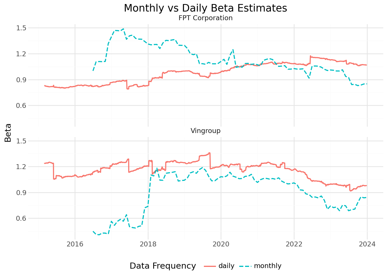
The comparison reveals that daily-based estimates are generally smoother due to the larger number of observations in each window. However, the level and trend of estimates are similar across frequencies, providing validation that both approaches capture the same underlying systematic risk exposure.
# Correlation between monthly and daily estimates
correlation_data = (beta_combined
    .pivot_table(index=["symbol", "date"], columns="frequency", values="beta")
    .dropna()
)

print(f"Correlation between monthly and daily betas: {correlation_data.corr().iloc[0,1]:.3f}")
Correlation between monthly and daily betas: 0.745| Factor | Effect |
|---|---|
| Non-synchronous trading | Daily betas can be biased downward for illiquid stocks |
| Microstructure noise | Bid-ask bounce adds noise to daily estimates |
| Different effective windows | Same calendar period but ~20x more observations for daily |
| Mean reversion speed | Daily captures faster-moving risk dynamics |
Table 15.1 shows several reasons why we might observe imperfect correlation.
15.10 Key Takeaways
CAPM beta measures a stock’s sensitivity to systematic market risk and is fundamental to modern portfolio theory, cost of capital estimation, and risk management.
Rolling-window estimation captures time variation in betas, which reflects changes in companies’ business models, leverage, and market conditions.
Parallelization dramatically reduces computation time for large-scale estimation tasks by distributing work across multiple CPU cores.
Estimation choices matter: Window length, return frequency, and minimum observation requirements all affect beta estimates. Researchers should choose parameters appropriate for their specific application.
Industry patterns: Vietnamese stocks show systematic differences in market sensitivity across industries, with cyclical sectors exhibiting higher betas than defensive sectors.
Time variation: The cross-sectional distribution of betas in Vietnam has evolved over time, with notable shifts during market stress periods.
Frequency comparison: Monthly and daily beta estimates are positively correlated but not identical. Daily estimates are smoother while monthly estimates may better capture lower-frequency variation.
Data quality checks: Coverage analysis and summary statistics help identify potential issues in estimation procedures before using results in downstream analyses.