import pandas as pd
import numpy as np
import matplotlib.pyplot as plt
import seaborn as sns
import statsmodels.api as sm
from statsmodels.regression.linear_model import OLS
from scipy import stats
from datetime import datetime, timedelta
from dateutil.relativedelta import relativedelta
import warnings

warnings.filterwarnings("ignore")

plt.rcParams.update({
    "figure.figsize": (10, 6),
    "font.size": 12,
    "axes.titlesize": 14,
    "axes.labelsize": 12,
    "xtick.labelsize": 10,
    "ytick.labelsize": 10,
    "legend.fontsize": 10,
    "figure.dpi": 150,
    "savefig.dpi": 300,
    "font.family": "serif",
})

sns.set_style("whitegrid")
np.random.seed(42)36 Return Gap: Measuring Unobserved Actions of Fund Managers
Mutual fund managers possess considerable discretion in their investment decisions between mandatory portfolio disclosure dates. While regulatory frameworks require periodic disclosure of holdings, the actions taken between these disclosure dates (e.g., trading, market timing, securities lending, and strategic cash management) remain largely unobservable to investors. These unobserved actions can significantly affect fund performance, either positively through skilled interim trading or negatively through agency costs and hidden behavior.
Kacperczyk, Sialm, and Zheng (2008) developed the Return Gap measure to capture the aggregate impact of these unobserved actions on fund returns. The Return Gap is defined as the difference between a fund’s actual reported return and the hypothetical return of a portfolio that mechanically invests in the fund’s most recently disclosed holdings. Formally:
\[ \text{Return Gap}_{i,t} = R_{i,t}^{\text{Actual}} - R_{i,t}^{\text{Holdings}} \tag{36.1}\]
where \(R_{i,t}^{\text{Actual}}\) is the net-of-expense return reported by fund \(i\) in month \(t\), adjusted for expenses to obtain the gross return, and \(R_{i,t}^{\text{Holdings}}\) is the hypothetical buy-and-hold return computed from the most recently disclosed portfolio holdings.
A positive Return Gap indicates that the fund manager’s unobserved actions (e.g., interim trading, cash management, or other activities) added value beyond what a passive replication of disclosed holdings would have generated. Conversely, a persistently negative Return Gap suggests value-destroying interim activity, potentially driven by agency costs, poor trading execution, or hidden fees.
36.1 Why Return Gap Matters
The Return Gap is economically significant for several reasons:
- Performance persistence: Funds in the highest Return Gap decile tend to outperform those in the lowest decile by 1-2% annually on a risk-adjusted basis, and this spread persists over time (Kacperczyk, Sialm, and Zheng 2008).
- Detecting agency problems: A persistently negative Return Gap can signal hidden costs such as excessive trading, market impact costs, soft-dollar arrangements, or stale-price exploitation.
- Complementing traditional measures: Unlike alpha-based metrics that blend stock selection skill with interim trading skill, the Return Gap isolates the component of performance attributable to actions taken between disclosure dates.
- Regulatory implications: In emerging markets like Vietnam, where disclosure frequency and regulatory oversight may differ from developed markets, the Return Gap can serve as an early warning system for investor protection.
36.2 Application to the Vietnamese Market
The Vietnamese mutual fund industry, while relatively young compared to the United States, has experienced rapid growth since the establishment of the first domestic equity funds in the early 2000s. As of 2024, Vietnam’s open-ended fund industry manages assets exceeding 100 trillion VND, with dozens of equity-oriented funds operated by both domestic and foreign-affiliated asset management companies.
Several characteristics of the Vietnamese market make the Return Gap analysis particularly interesting:
- Disclosure frequency: Vietnamese funds are required to disclose their top holdings periodically, but the frequency and completeness of disclosure may differ from the quarterly SEC requirements in the U.S.
- Market microstructure: The HOSE (Ho Chi Minh Stock Exchange) and HNX (Hanoi Stock Exchange) feature daily price limits (plus or minus 7% on HOSE, plus or minus 10% on HNX), T+2 settlement, and foreign ownership limits that may constrain or enable certain interim trading strategies.
- Information asymmetry: In an emerging market with less analyst coverage, the scope for informed interim trading and hence positive Return Gap may be larger than in more efficient markets.
- Regulatory environment: Vietnam’s State Securities Commission (SSC) has progressively strengthened disclosure and governance requirements, making temporal analysis of Return Gap especially informative.
37 Theoretical Framework
37.1 Decomposing Fund Returns
Consider a mutual fund \(i\) that discloses its portfolio holdings at discrete dates \(\tau_1, \tau_2, \ldots\) As disclosed at date \(\tau_k\), the fund holds \(N_k\) securities with weights \(\{w_{j,\tau_k}\}_{j=1}^{N_k}\), where \(w_{j,\tau_k}\) represents the portfolio weight of security \(j\).
Between disclosure dates \(\tau_k\) and \(\tau_{k+1}\), the fund’s actual gross return in month \(t\) can be decomposed as:
\[ R_{i,t}^{\text{Gross}} = R_{i,t}^{\text{Holdings}} + \underbrace{R_{i,t}^{\text{Gross}} - R_{i,t}^{\text{Holdings}}}_{\text{Return Gap}} \tag{37.1}\]
The hypothetical holdings return \(R_{i,t}^{\text{Holdings}}\) is computed as the value-weighted return of the buy-and-hold portfolio based on the most recent disclosure:
\[ R_{i,t}^{\text{Holdings}} = \sum_{j=1}^{N_k} \tilde{w}_{j,t-1} \cdot r_{j,t} \tag{37.2}\]
where \(r_{j,t}\) is the return of security \(j\) in month \(t\), and \(\tilde{w}_{j,t-1}\) is the evolved portfolio weight at the end of month \(t-1\), reflecting the buy-and-hold drift from the original disclosure weights:
\[ \tilde{w}_{j,t-1} = \frac{w_{j,\tau_k} \prod_{s=\tau_k+1}^{t-1}(1 + r_{j,s})}{\sum_{\ell=1}^{N_k} w_{\ell,\tau_k} \prod_{s=\tau_k+1}^{t-1}(1 + r_{\ell,s})} \tag{37.3}\]
In practice, rather than tracking evolved weights explicitly, we use dollar values of holdings positions (shares held times price) as the natural weighting scheme.
37.2 The Return Gap Measure
37.2.1 Gross Return Gap
The Return Gap as originally defined by Kacperczyk, Sialm, and Zheng (2008) uses the gross (before-expense) return:
\[ \text{RG}_{i,t} = R_{i,t}^{\text{Gross}} - R_{i,t}^{\text{Holdings}} = \left(R_{i,t}^{\text{Net}} + \frac{\text{Expense Ratio}_{i,t}}{12}\right) - R_{i,t}^{\text{Holdings}} \tag{37.4}\]
where \(R_{i,t}^{\text{Net}}\) is the reported net-of-expense return and the annual expense ratio is divided by 12 to approximate the monthly expense charge.
37.2.2 Sources of Return Gap
The Return Gap captures several components (Kacperczyk, Sialm, and Zheng 2008; Elton, Gruber, and Blake 2011):
\[ \text{RG}_{i,t} = \underbrace{\Delta_{\text{trade}}}_{\text{Interim trading}} + \underbrace{\Delta_{\text{cash}}}_{\text{Cash drag/return}} + \underbrace{\Delta_{\text{fees}}}_{\text{Hidden fees}} + \underbrace{\Delta_{\text{lend}}}_{\text{Securities lending}} + \underbrace{\varepsilon_t}_{\text{Noise}} \tag{37.5}\]
where:
- \(\Delta_{\text{trade}}\): The return impact of buying and selling securities between disclosure dates. Skilled managers generate positive \(\Delta_{\text{trade}}\) by timing trades.
- \(\Delta_{\text{cash}}\): The effect of holding cash or cash equivalents not captured in equity holdings disclosures. In rising markets, cash creates a drag (negative contribution); in falling markets, cash provides a cushion.
- \(\Delta_{\text{fees}}\): Transaction costs, brokerage commissions, and any hidden fees not reflected in the stated expense ratio.
- \(\Delta_{\text{lend}}\): Revenue from securities lending programs, which generates positive Return Gap.
- \(\varepsilon_t\): Measurement noise from timing differences, stale prices, or data errors.
37.2.3 Predictive Return Gap
To form tradeable portfolios and avoid look-ahead bias, Kacperczyk, Sialm, and Zheng (2008) use the trailing 12-month average Return Gap, lagged by one quarter to account for the reporting delay:
\[ \overline{\text{RG}}_{i,t}^{12} = \frac{1}{12} \sum_{s=1}^{12} \text{RG}_{i,t-s} \tag{37.6}\]
The additional 3-month (one quarter) lag ensures that the Return Gap signal is based only on information available to investors at the time of portfolio formation. This is particularly important in Vietnam, where fund reporting may involve delays.
37.3 Risk-Adjusted Performance Evaluation
To evaluate whether Return Gap-sorted portfolios generate genuine risk-adjusted returns, we employ several factor models.
37.3.1 CAPM Alpha
\[ R_{p,t} - R_{f,t} = \alpha_p + \beta_p (R_{m,t} - R_{f,t}) + \epsilon_{p,t} \tag{37.7}\]
37.3.2 Fama-French Three-Factor Model
\[ R_{p,t} - R_{f,t} = \alpha_p + \beta_{1,p} \cdot \text{MKT}_t + \beta_{2,p} \cdot \text{SMB}_t + \beta_{3,p} \cdot \text{HML}_t + \epsilon_{p,t} \tag{37.8}\]
37.3.3 Carhart Four-Factor Model
\[ R_{p,t} - R_{f,t} = \alpha_p + \beta_{1,p} \cdot \text{MKT}_t + \beta_{2,p} \cdot \text{SMB}_t + \beta_{3,p} \cdot \text{HML}_t + \beta_{4,p} \cdot \text{UMD}_t + \epsilon_{p,t} \tag{37.9}\]
where \(\text{UMD}_t\) is the momentum factor (up minus down).
37.3.4 Fama-French Five-Factor Model
For a more comprehensive risk adjustment relevant to the Vietnamese market:
\[ R_{p,t} - R_{f,t} = \alpha_p + \beta_1 \text{MKT}_t + \beta_2 \text{SMB}_t + \beta_3 \text{HML}_t + \beta_4 \text{RMW}_t + \beta_5 \text{CMA}_t + \epsilon_{p,t} \tag{37.10}\]
where \(\text{RMW}_t\) (robust minus weak) captures profitability and \(\text{CMA}_t\) (conservative minus aggressive) captures investment patterns.
37.4 Newey-West Standard Errors
Since portfolio returns may exhibit serial correlation, we use Newey and West (1987) standard errors with \(L\) lags:
\[ \hat{V}(\hat{\alpha}) = T \left(\sum_{t=1}^{T} \mathbf{x}_t \mathbf{x}_t'\right)^{-1} \hat{S} \left(\sum_{t=1}^{T} \mathbf{x}_t \mathbf{x}_t'\right)^{-1} \tag{37.11}\]
where the HAC covariance estimator is:
\[ \hat{S} = \hat{\Gamma}_0 + \sum_{\ell=1}^{L} \left(1 - \frac{\ell}{L+1}\right)\left(\hat{\Gamma}_\ell + \hat{\Gamma}_\ell'\right) \tag{37.12}\]
and \(\hat{\Gamma}_\ell = \frac{1}{T}\sum_{t=\ell+1}^{T} \hat{\epsilon}_t \hat{\epsilon}_{t-\ell} \mathbf{x}_t \mathbf{x}_{t-\ell}'\). The standard lag choice is \(L = \lfloor 4(T/100)^{2/9} \rfloor\).
38 Data and Sample Construction
38.1 Data Sources
Table 38.1 shows the sources used in the construction of return gaps.
| Data Category | Source | Description |
|---|---|---|
| Fund holdings | DataCore Fund Holdings | Disclosed portfolio positions including ticker, shares held, report date, and vintage (filing) date |
| Fund returns | DataCore Fund Performance | Monthly NAV-based net returns, total net assets, and expense ratios |
| Fund characteristics | DataCore Fund Master | Fund objective codes, inception dates, management company, investment style |
| Stock prices and returns | DataCore Equity Market | Daily and monthly adjusted prices, returns, shares outstanding, and corporate actions for HOSE and HNX listed securities |
| Risk factors | DataCore / Constructed | Vietnamese market factor portfolios (MKT, SMB, HML, UMD, RMW, CMA) |
38.2 Setting Up the Environment
38.3 Loading and Preparing Stock Market Data
The first step is to load the stock-level data, which provides the foundation for computing hypothetical holdings returns.
# ============================================================
# In production, replace with actual DataCore API calls:
#   from datacore import DataCoreClient
#   client = DataCoreClient(api_key="YOUR_KEY")
#   stock_data = client.get_equity_monthly(
#       exchange=["HOSE", "HNX"],
#       start_date="2010-01-01",
#       end_date="2024-12-31",
#       fields=["ticker", "date", "close_adj", "return_monthly",
#               "shares_outstanding", "market_cap"]
#   )
# ============================================================

def generate_stock_data(
    n_stocks: int = 300,
    start_date: str = "2012-01-01",
    end_date: str = "2024-12-31",
) -> pd.DataFrame:
    """
    Generate simulated monthly stock data mimicking Vietnamese
    equity market characteristics.
    """
    dates = pd.date_range(start_date, end_date, freq="ME")
    tickers = [f"VN{str(i).zfill(4)}" for i in range(1, n_stocks + 1)]

    records = []
    for ticker in tickers:
        list_offset = np.random.randint(0, max(1, len(dates) // 3))
        available_dates = dates[list_offset:]
        mu = np.random.normal(0.008, 0.005)
        sigma = np.random.uniform(0.06, 0.15)
        beta = np.random.uniform(0.5, 1.8)
        market_shocks = np.random.normal(0.005, 0.06, len(available_dates))
        idio_shocks = np.random.normal(0, sigma, len(available_dates))
        returns = mu + beta * market_shocks + idio_shocks
        returns = np.clip(returns, -0.30, 0.40)
        price = np.random.uniform(10, 150)
        prices = [price]
        for r in returns[:-1]:
            price = price * (1 + r)
            prices.append(price)
        shares = np.random.uniform(50, 500) * 1e6
        shares_series = np.full(len(available_dates), shares)
        for i, d in enumerate(available_dates):
            records.append({
                "ticker": ticker, "date": d,
                "close_adj": prices[i], "ret": returns[i],
                "shares_outstanding": shares_series[i],
                "market_cap": prices[i] * shares_series[i] / 1e9,
            })

    df = pd.DataFrame(records)
    df["date"] = pd.to_datetime(df["date"])
    df = df.sort_values(["ticker", "date"])
    df["close_adj_lag"] = df.groupby("ticker")["close_adj"].shift(1)
    return df

stock_data = generate_stock_data()
print(f"Stock data: {stock_data.shape[0]:,} stock-months")
print(f"Unique stocks: {stock_data['ticker'].nunique()}")
print(f"Date range: {stock_data['date'].min():%Y-%m} to "
      f"{stock_data['date'].max():%Y-%m}")
stock_data.head(10)
Stock data: 38,865 stock-months
Unique stocks: 300
Date range: 2012-01 to 2024-12| ticker | date | close_adj | ret | shares_outstanding | market_cap | close_adj_lag | |
|---|---|---|---|---|---|---|---|
| 0 | VN0001 | 2015-03-31 | 45.035190 | 0.110630 | 6.747563e+07 | 3.038778 | NaN |
| 1 | VN0001 | 2015-04-30 | 50.017423 | -0.066939 | 6.747563e+07 | 3.374957 | 45.035190 |
| 2 | VN0001 | 2015-05-31 | 46.669311 | 0.047021 | 6.747563e+07 | 3.149041 | 50.017423 |
| 3 | VN0001 | 2015-06-30 | 48.863751 | -0.152745 | 6.747563e+07 | 3.297112 | 46.669311 |
| 4 | VN0001 | 2015-07-31 | 41.400073 | -0.057519 | 6.747563e+07 | 2.793496 | 48.863751 |
| 5 | VN0001 | 2015-08-31 | 39.018788 | 0.228286 | 6.747563e+07 | 2.632817 | 41.400073 |
| 6 | VN0001 | 2015-09-30 | 47.926227 | 0.079232 | 6.747563e+07 | 3.233852 | 39.018788 |
| 7 | VN0001 | 2015-10-31 | 51.723515 | -0.300000 | 6.747563e+07 | 3.490077 | 47.926227 |
| 8 | VN0001 | 2015-11-30 | 36.206461 | 0.192114 | 6.747563e+07 | 2.443054 | 51.723515 |
| 9 | VN0001 | 2015-12-31 | 43.162239 | 0.294336 | 6.747563e+07 | 2.912399 | 36.206461 |
38.4 Loading Fund Holdings Data
def generate_holdings_data(
    stock_data: pd.DataFrame,
    n_funds: int = 50,
    start_date: str = "2012-06-30",
    end_date: str = "2024-12-31",
) -> pd.DataFrame:
    """
    Generate simulated fund holdings data. Each fund holds 15-80
    stocks, disclosed semi-annually or quarterly.
    """
    dates = pd.date_range(start_date, end_date, freq="ME")
    tickers = stock_data["ticker"].unique()
    fund_ids = [f"FUND{str(i).zfill(3)}" for i in range(1, n_funds + 1)]
    records = []
    for fund_id in fund_ids:
        inception_idx = np.random.randint(0, max(1, len(dates) // 4))
        freq = 3 if np.random.random() < 0.7 else 6
        n_stocks_held = np.random.randint(15, 80)
        core_stocks = np.random.choice(tickers, size=n_stocks_held, replace=False)
        report_dates = dates[inception_idx::freq]
        for rdate in report_dates:
            filing_delay = np.random.randint(1, 4)
            fdate = rdate + pd.DateOffset(months=filing_delay)
            turnover = np.random.uniform(0.05, 0.20)
            n_replace = max(1, int(n_stocks_held * turnover))
            replace_idx = np.random.choice(len(core_stocks), size=n_replace, replace=False)
            new_stocks = np.random.choice(tickers, size=n_replace, replace=False)
            core_stocks[replace_idx] = new_stocks
            for ticker in core_stocks:
                shares = np.random.uniform(100_000, 5_000_000)
                records.append({
                    "fund_id": fund_id, "report_date": rdate,
                    "filing_date": fdate, "ticker": ticker,
                    "shares_held": shares,
                })
    df = pd.DataFrame(records)
    df["report_date"] = pd.to_datetime(df["report_date"])
    df["filing_date"] = pd.to_datetime(df["filing_date"])
    return df

holdings_raw = generate_holdings_data(stock_data)
print(f"Holdings records: {holdings_raw.shape[0]:,}")
print(f"Unique funds: {holdings_raw['fund_id'].nunique()}")
holdings_raw.head(10)
Holdings records: 89,269
Unique funds: 50| fund_id | report_date | filing_date | ticker | shares_held | |
|---|---|---|---|---|---|
| 0 | FUND001 | 2012-11-30 | 2012-12-30 | VN0289 | 4.918132e+06 |
| 1 | FUND001 | 2012-11-30 | 2012-12-30 | VN0297 | 4.322425e+05 |
| 2 | FUND001 | 2012-11-30 | 2012-12-30 | VN0259 | 2.383117e+05 |
| 3 | FUND001 | 2012-11-30 | 2012-12-30 | VN0215 | 1.140891e+06 |
| 4 | FUND001 | 2012-11-30 | 2012-12-30 | VN0262 | 1.104603e+06 |
| 5 | FUND001 | 2012-11-30 | 2012-12-30 | VN0292 | 1.665416e+06 |
| 6 | FUND001 | 2012-11-30 | 2012-12-30 | VN0132 | 4.625400e+06 |
| 7 | FUND001 | 2012-11-30 | 2012-12-30 | VN0049 | 3.447053e+06 |
| 8 | FUND001 | 2012-11-30 | 2012-12-30 | VN0008 | 1.525004e+05 |
| 9 | FUND001 | 2012-11-30 | 2012-12-30 | VN0189 | 2.527258e+06 |
38.5 Loading Fund Returns and Characteristics
def generate_fund_returns(holdings, start_date="2012-01-01", end_date="2024-12-31"):
    """Generate monthly fund-level net returns, TNA, and expense ratios."""
    fund_ids = holdings["fund_id"].unique()
    dates = pd.date_range(start_date, end_date, freq="ME")
    records = []
    for fund_id in fund_ids:
        fund_start = holdings.loc[holdings["fund_id"] == fund_id, "report_date"].min() - pd.DateOffset(months=3)
        fund_dates = dates[dates >= fund_start]
        exp_ratio = np.random.uniform(0.010, 0.025)
        base_tna = np.random.uniform(50, 2000)
        mu = np.random.normal(0.007, 0.003)
        sigma = np.random.uniform(0.04, 0.09)
        tna = base_tna
        for d in fund_dates:
            ret = np.clip(np.random.normal(mu, sigma), -0.25, 0.35)
            tna = max(tna * (1 + ret) + np.random.normal(0, base_tna * 0.02), 10)
            records.append({"fund_id": fund_id, "date": d, "net_return": ret,
                            "tna": tna, "expense_ratio": exp_ratio + np.random.normal(0, 0.001)})
    df = pd.DataFrame(records)
    df["date"] = pd.to_datetime(df["date"])
    df["expense_ratio"] = df["expense_ratio"].clip(0.005, 0.035)
    return df

fund_returns = generate_fund_returns(holdings_raw)
print(f"Fund-month observations: {fund_returns.shape[0]:,}")
fund_returns.head(10)
Fund-month observations: 6,808| fund_id | date | net_return | tna | expense_ratio | |
|---|---|---|---|---|---|
| 0 | FUND001 | 2012-08-31 | 0.045634 | 568.611866 | 0.022429 |
| 1 | FUND001 | 2012-09-30 | 0.106959 | 631.630643 | 0.021461 |
| 2 | FUND001 | 2012-10-31 | -0.063495 | 612.614200 | 0.020634 |
| 3 | FUND001 | 2012-11-30 | -0.087247 | 563.095634 | 0.023795 |
| 4 | FUND001 | 2012-12-31 | -0.006777 | 545.547597 | 0.021886 |
| 5 | FUND001 | 2013-01-31 | -0.029553 | 532.221482 | 0.021999 |
| 6 | FUND001 | 2013-02-28 | -0.002767 | 538.411988 | 0.021567 |
| 7 | FUND001 | 2013-03-31 | -0.138187 | 477.997478 | 0.022189 |
| 8 | FUND001 | 2013-04-30 | 0.045137 | 484.711443 | 0.022058 |
| 9 | FUND001 | 2013-05-31 | 0.095518 | 523.213577 | 0.021911 |
38.6 Sample Selection: Domestic Equity Funds
Following the approach of Kacperczyk, Sialm, and Zheng (2008), we restrict our sample to domestic equity funds.
equity_objectives = [
    "EQUITY_DOMESTIC", "EQUITY_GROWTH", "EQUITY_VALUE",
    "EQUITY_BLEND", "EQUITY_LARGE_CAP", "EQUITY_MID_CAP",
    "EQUITY_SMALL_CAP",
]

fund_ids = fund_returns["fund_id"].unique()
fund_master = pd.DataFrame({
    "fund_id": fund_ids,
    "objective": np.random.choice(
        equity_objectives + ["BOND", "BALANCED", "MONEY_MARKET"],
        size=len(fund_ids),
        p=[0.08, 0.08, 0.06, 0.10, 0.08, 0.06, 0.06, 0.15, 0.18, 0.15],
    ),
})

equity_fund_ids = fund_master.loc[
    fund_master["objective"].isin(equity_objectives), "fund_id"
].values

print(f"Total funds: {len(fund_ids)}")
print(f"Equity funds: {len(equity_fund_ids)} ({len(equity_fund_ids)/len(fund_ids)*100:.1f}%)")
print("\nObjective distribution:")
print(fund_master["objective"].value_counts().to_string())
Total funds: 50
Equity funds: 29 (58.0%)
Objective distribution:
objective
BALANCED 9
EQUITY_VALUE 9
EQUITY_GROWTH 6
BOND 6
MONEY_MARKET 6
EQUITY_BLEND 5
EQUITY_LARGE_CAP 3
EQUITY_SMALL_CAP 2
EQUITY_MID_CAP 2
EQUITY_DOMESTIC 239 Computing the Return Gap
39.1 Step 1: Prepare Holdings Vintages
A critical first step is to correctly handle the vintage structure of holdings data. Each holdings report has two key dates: the report date (\(\tau\), the as-of date) and the filing date (\(f\), when it becomes public). We keep only the first vintage per fund-report date.
def prepare_holdings_vintages(holdings, max_holding_months=6):
    """Process holdings vintages and compute next report dates."""
    first_vintage = (
        holdings.sort_values(["fund_id", "report_date", "filing_date"])
        .groupby(["fund_id", "report_date"])
        .agg(filing_date=("filing_date", "first"))
        .reset_index()
    )
    first_vintage = first_vintage.sort_values(["fund_id", "report_date"])
    first_vintage["next_report_date"] = first_vintage.groupby("fund_id")["report_date"].shift(-1)
    max_date = first_vintage["report_date"] + pd.DateOffset(months=max_holding_months)
    first_vintage["next_report_date"] = first_vintage["next_report_date"].fillna(max_date)
    first_vintage["next_report_date"] = first_vintage[["next_report_date"]].min(axis=1).clip(upper=max_date)
    first_vintage["next_report_date"] = first_vintage["next_report_date"] + pd.offsets.MonthEnd(0)
    result = holdings.merge(first_vintage, on=["fund_id", "report_date", "filing_date"], how="inner")
    return result

holdings_vintaged = prepare_holdings_vintages(holdings_raw)
print(f"Holdings after vintage processing: {holdings_vintaged.shape[0]:,} records")
sample_fund = holdings_vintaged["fund_id"].iloc[0]
(holdings_vintaged.loc[holdings_vintaged["fund_id"] == sample_fund]
 [["fund_id", "report_date", "filing_date", "next_report_date"]]
 .drop_duplicates().head(8))
Holdings after vintage processing: 89,269 records| fund_id | report_date | filing_date | next_report_date | |
|---|---|---|---|---|
| 0 | FUND001 | 2012-11-30 | 2012-12-30 | 2013-02-28 |
| 52 | FUND001 | 2013-02-28 | 2013-03-28 | 2013-05-31 |
| 104 | FUND001 | 2013-05-31 | 2013-08-31 | 2013-08-31 |
| 156 | FUND001 | 2013-08-31 | 2013-11-30 | 2013-11-30 |
| 208 | FUND001 | 2013-11-30 | 2014-02-28 | 2014-02-28 |
| 260 | FUND001 | 2014-02-28 | 2014-04-28 | 2014-05-31 |
| 312 | FUND001 | 2014-05-31 | 2014-08-31 | 2014-08-31 |
| 364 | FUND001 | 2014-08-31 | 2014-10-31 | 2014-11-30 |
39.3 Step 3: Compute Hypothetical Holdings Returns
This is the core computation. For each fund, we take the disclosed holdings as of report date \(\tau\), and for each month \(t\) in \((\tau, \tau_{\text{next}}]\), compute the value-weighted return using lagged dollar values as weights.
def compute_holdings_returns(holdings, stock_data, min_stocks=10, min_assets_bn=5.0):
    """Compute monthly hypothetical buy-and-hold portfolio returns."""
    merged = holdings.merge(stock_data, on="ticker", how="inner")
    mask = (merged["date"] > merged["report_date"]) & (merged["date"] <= merged["next_report_date"])
    merged = merged.loc[mask].copy()
    merged["hvalue_lag"] = merged["shares_adj"] * merged["close_adj_lag"]
    merged = merged.loc[merged["hvalue_lag"] > 0].copy()
    merged = merged.drop_duplicates(subset=["fund_id", "date", "report_date", "ticker"], keep="first")

    def weighted_return(group):
        weights = group["hvalue_lag"]
        total_weight = weights.sum()
        if total_weight <= 0:
            return pd.Series({"hret": np.nan, "n_stocks": 0, "assets_lag_bn": 0})
        wret = np.average(group["ret"], weights=weights)
        return pd.Series({"hret": wret, "n_stocks": len(group), "assets_lag_bn": total_weight / 1e9})

    portfolio_returns = (
        merged.groupby(["fund_id", "date"])
        .apply(weighted_return, include_groups=False).reset_index()
    )
    portfolio_returns["assets_bn"] = portfolio_returns["assets_lag_bn"] * (1 + portfolio_returns["hret"])
    mask = (portfolio_returns["n_stocks"] >= min_stocks) & (portfolio_returns["assets_bn"] >= min_assets_bn)
    return portfolio_returns.loc[mask].copy()

holdings_returns = compute_holdings_returns(holdings_adj, stock_data)
print(f"Fund-month observations (hypothetical returns): {holdings_returns.shape[0]:,}")
print(f"Unique funds: {holdings_returns['fund_id'].nunique()}")
print(f"\nSummary:")
print(holdings_returns[["hret", "n_stocks", "assets_bn"]].describe().round(4).to_string())
Fund-month observations (hypothetical returns): 6,170
Unique funds: 50
Summary:
hret n_stocks assets_bn
count 6170.0000 6170.0000 6170.0000
mean 0.0149 42.7476 27.8827
std 0.0426 14.5061 20.1749
min -0.1997 13.0000 5.0241
25% -0.0111 31.0000 13.3775
50% 0.0146 41.0000 22.6388
75% 0.0411 53.0000 35.6065
max 0.2209 74.0000 167.351139.4 Step 4: Compute Gross Fund Returns
def prepare_fund_returns(fund_returns, equity_fund_ids):
    """Prepare fund-level gross returns."""
    df = fund_returns.loc[fund_returns["fund_id"].isin(equity_fund_ids)].copy()
    df["expense_ratio"] = df["expense_ratio"].fillna(df.groupby("fund_id")["expense_ratio"].transform("median"))
    df["gross_return"] = df["net_return"] + df["expense_ratio"] / 12
    df = df.sort_values(["fund_id", "date"])
    df["tna_lag"] = df.groupby("fund_id")["tna"].shift(1).fillna(df["tna"])
    return df

fund_ret_clean = prepare_fund_returns(fund_returns, equity_fund_ids)
print(f"Equity fund-months: {fund_ret_clean.shape[0]:,}")
Equity fund-months: 3,99339.5 Step 5: Merge and Compute Return Gap
def compute_return_gap(holdings_returns, fund_returns):
    """Compute Return Gap and trailing averages."""
    merged = holdings_returns.merge(
        fund_returns[["fund_id", "date", "net_return", "gross_return", "expense_ratio", "tna"]],
        on=["fund_id", "date"], how="inner",
    )
    merged["return_gap"] = merged["gross_return"] - merged["hret"]
    merged = merged.sort_values(["fund_id", "date"])
    merged["rg_12m"] = merged.groupby("fund_id")["return_gap"].transform(
        lambda x: x.rolling(12, min_periods=8).mean()
    )
    merged["rg_12m_lag4"] = merged.groupby("fund_id")["rg_12m"].shift(4)
    return merged

return_gap_data = compute_return_gap(holdings_returns, fund_ret_clean)
print(f"Return Gap observations: {return_gap_data.shape[0]:,}")
print(f"\nSummary:")
print(return_gap_data[["return_gap", "rg_12m", "rg_12m_lag4"]].describe().round(6).to_string())
Return Gap observations: 3,592
Summary:
return_gap rg_12m rg_12m_lag4
count 3592.000000 3389.000000 3273.000000
mean -0.005734 -0.005349 -0.005329
std 0.080211 0.022955 0.022864
min -0.307136 -0.094187 -0.094187
25% -0.058760 -0.019080 -0.019057
50% -0.006127 -0.005284 -0.005242
75% 0.047785 0.008620 0.008653
max 0.277137 0.079589 0.07958939.6 Distribution of the Return Gap
fig, axes = plt.subplots(1, 2, figsize=(12, 5))

rg = return_gap_data["return_gap"].dropna()
rg_trimmed = rg.clip(rg.quantile(0.01), rg.quantile(0.99))
axes[0].hist(rg_trimmed, bins=80, density=True, alpha=0.7, color="#2C5F8A", edgecolor="white", linewidth=0.5)
axes[0].axvline(rg.mean(), color="#D32F2F", linestyle="--", linewidth=2, label=f"Mean = {rg.mean():.4f}")
axes[0].axvline(rg.median(), color="#FF8F00", linestyle="-.", linewidth=2, label=f"Median = {rg.median():.4f}")
axes[0].set_xlabel("Monthly Return Gap")
axes[0].set_ylabel("Density")
axes[0].set_title("Panel A: Monthly Return Gap")
axes[0].legend(frameon=True)

rg12 = return_gap_data["rg_12m"].dropna()
rg12_trimmed = rg12.clip(rg12.quantile(0.01), rg12.quantile(0.99))
axes[1].hist(rg12_trimmed, bins=80, density=True, alpha=0.7, color="#1B5E20", edgecolor="white", linewidth=0.5)
axes[1].axvline(rg12.mean(), color="#D32F2F", linestyle="--", linewidth=2, label=f"Mean = {rg12.mean():.4f}")
axes[1].axvline(rg12.median(), color="#FF8F00", linestyle="-.", linewidth=2, label=f"Median = {rg12.median():.4f}")
axes[1].set_xlabel("Trailing 12-Month Average Return Gap")
axes[1].set_ylabel("Density")
axes[1].set_title("Panel B: 12-Month Average Return Gap")
axes[1].legend(frameon=True)
plt.tight_layout()
plt.show()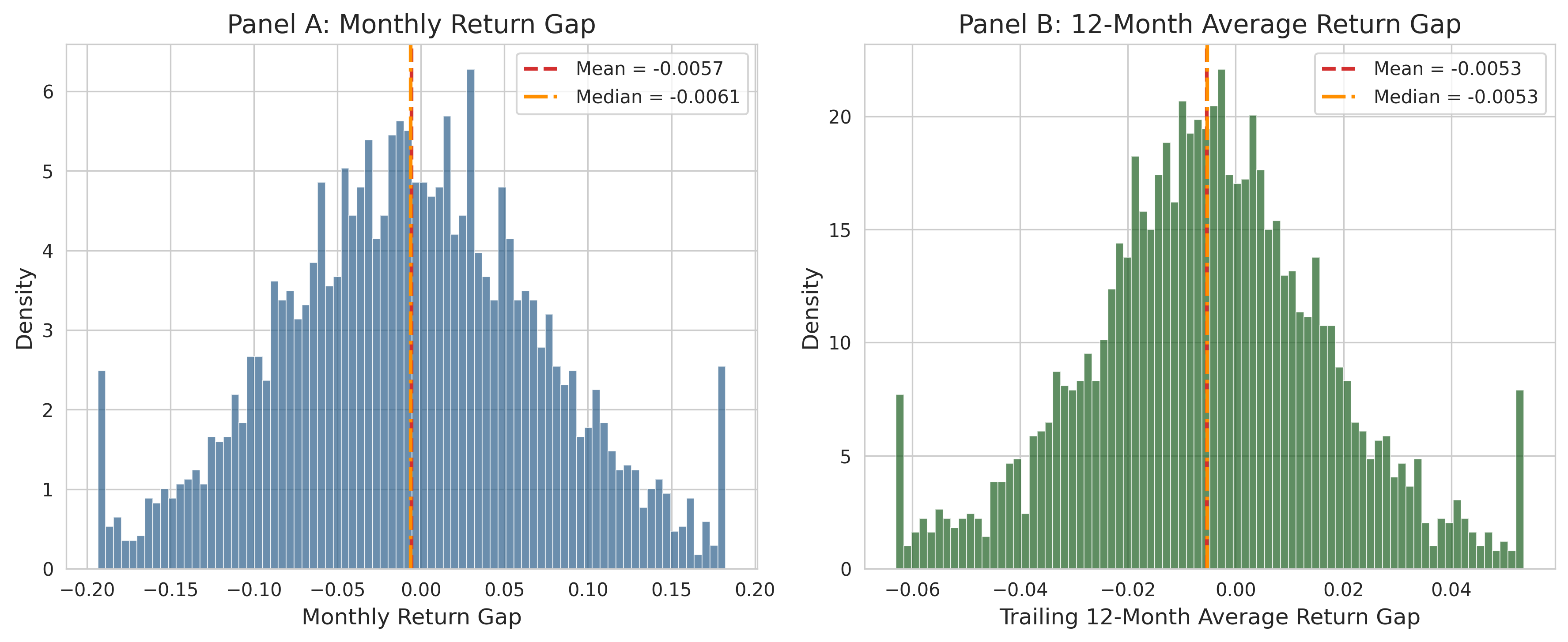
39.7 Time Series of Cross-Sectional Return Gap
ts_stats = (
    return_gap_data.groupby("date")["return_gap"]
    .agg(["mean", "median", lambda x: x.quantile(0.25), lambda x: x.quantile(0.75)])
    .rename(columns={"<lambda_0>": "p25", "<lambda_1>": "p75"}).reset_index()
)

fig, ax = plt.subplots(figsize=(12, 5))
ax.fill_between(ts_stats["date"], ts_stats["p25"], ts_stats["p75"], alpha=0.3, color="#2C5F8A", label="IQR")
ax.plot(ts_stats["date"], ts_stats["median"], color="#2C5F8A", linewidth=2, label="Median")
ax.plot(ts_stats["date"], ts_stats["mean"], color="#D32F2F", linestyle="--", linewidth=1.5, label="Mean")
ax.axhline(0, color="black", linewidth=0.8)
ax.set_xlabel("Date")
ax.set_ylabel("Monthly Return Gap")
ax.set_title("Cross-Sectional Distribution of Return Gap Over Time")
ax.legend(frameon=True)
plt.tight_layout()
plt.show()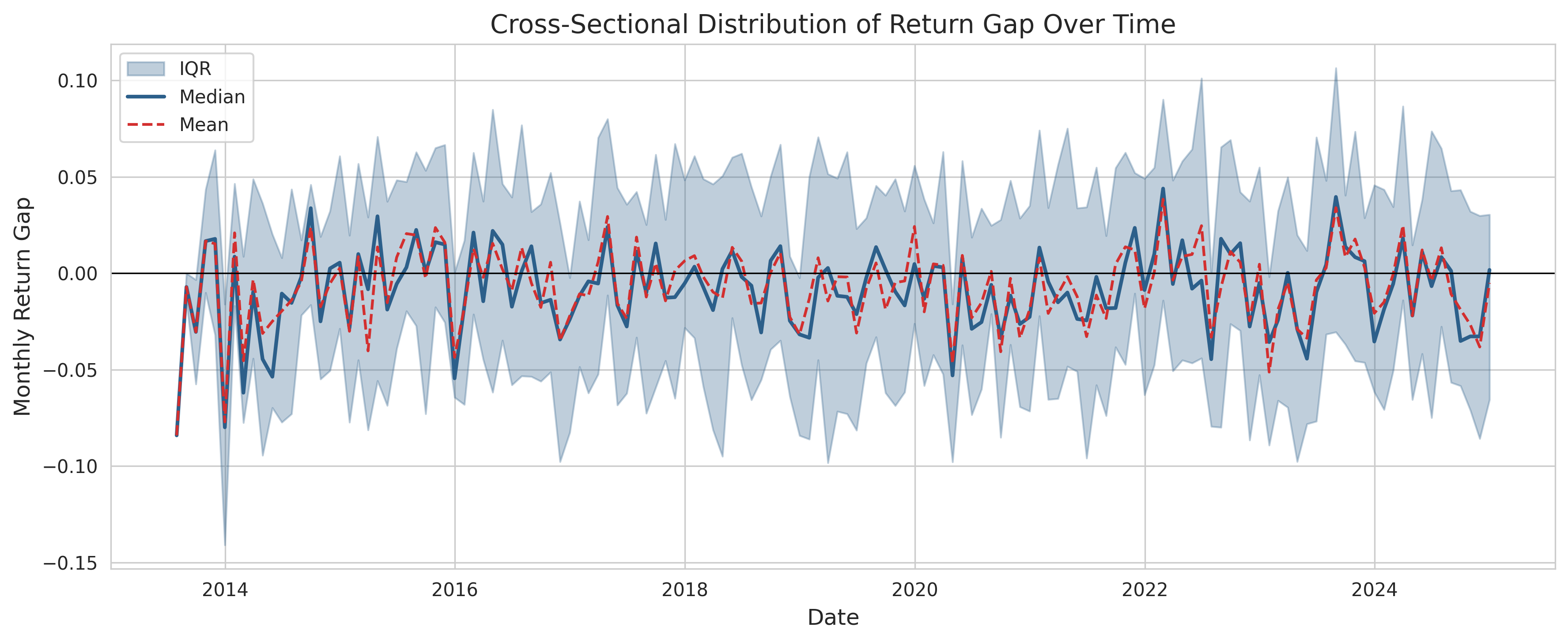
40 Portfolio Sorting Analysis
40.1 Forming Return Gap Decile Portfolios
Each month \(t\), we sort funds into decile portfolios based on their lagged 12-month average Return Gap (\(\overline{\text{RG}}_{i,t-4}^{12}\)). Portfolio 1 contains funds with the lowest Return Gap.
def form_return_gap_portfolios(data, n_portfolios=10, sort_var="rg_12m_lag4"):
    """Form portfolios by sorting funds into quantile groups."""
    df = data.dropna(subset=[sort_var]).copy()
    df["portfolio"] = (
        df.groupby("date")[sort_var]
        .transform(lambda x: pd.qcut(x, n_portfolios, labels=False, duplicates="drop"))
    ) + 1
    return df

n_portfolios = 10
portfolio_data = form_return_gap_portfolios(return_gap_data, n_portfolios=n_portfolios)
print(f"Observations with portfolio assignment: {portfolio_data.shape[0]:,}")
Observations with portfolio assignment: 3,27340.2 Portfolio Returns
def compute_portfolio_returns(data, n_portfolios=10):
    """Compute equal- and value-weighted monthly returns."""
    ew = data.groupby(["date", "portfolio"]).agg(
        ew_ret=("net_return", "mean"), n_funds=("fund_id", "count")).reset_index()
    def vw_func(group):
        w = group["tna"].clip(lower=0)
        return np.average(group["net_return"], weights=w) if w.sum() > 0 else group["net_return"].mean()
    vw = data.groupby(["date", "portfolio"]).apply(vw_func, include_groups=False).reset_index(name="vw_ret")
    return ew.merge(vw, on=["date", "portfolio"], how="left")

port_returns = compute_portfolio_returns(portfolio_data)
port_wide = port_returns.pivot_table(index="date", columns="portfolio", values=["ew_ret", "vw_ret"])
port_wide[("ew_ret", "LS")] = port_wide[("ew_ret", n_portfolios)] - port_wide[("ew_ret", 1)]
port_wide[("vw_ret", "LS")] = port_wide[("vw_ret", n_portfolios)] - port_wide[("vw_ret", 1)]

print("EW portfolio returns (annualized, %):")
print((port_wide["ew_ret"].mean() * 12 * 100).round(2).to_string())
EW portfolio returns (annualized, %):
portfolio
1.0 4.42
2.0 12.09
3.0 15.52
4.0 8.35
5.0 10.31
6.0 14.38
7.0 1.18
8.0 10.99
9.0 1.33
10.0 15.19
LS 10.7740.3 Characteristics of Return Gap Portfolios
chars = portfolio_data.groupby("portfolio").agg(
    avg_rg=("return_gap", "mean"), avg_rg12=("rg_12m_lag4", "mean"),
    avg_net_ret=("net_return", "mean"), avg_gross_ret=("gross_return", "mean"),
    avg_hret=("hret", "mean"), avg_expense=("expense_ratio", "mean"),
    avg_tna=("tna", "mean"), avg_nstocks=("n_stocks", "mean"), n_obs=("fund_id", "count"),
).round(4)
dc = chars.copy()
dc.columns = ["Avg RG", "Avg RG(12m)", "Net Ret", "Gross Ret", "Hold Ret", "Expense", "TNA(Bn)", "#Stocks", "#Obs"]
for col in ["Avg RG", "Avg RG(12m)", "Net Ret", "Gross Ret", "Hold Ret", "Expense"]:
    dc[col] = (dc[col] * 100).round(3)
dc["TNA(Bn)"] = dc["TNA(Bn)"].round(1)
dc["#Stocks"] = dc["#Stocks"].round(1)
print(dc.to_string())
Avg RG Avg RG(12m) Net Ret Gross Ret Hold Ret Expense TNA(Bn) #Stocks #Obs
portfolio
1.0 -0.81 -4.32 0.50 0.66 1.48 1.91 1395.7 41.9 353
2.0 0.16 -2.73 1.02 1.18 1.02 1.86 1941.3 43.9 333
3.0 0.06 -1.85 1.27 1.42 1.36 1.79 2042.0 45.5 335
4.0 -1.11 -1.22 0.51 0.66 1.78 1.81 2052.1 47.6 325
5.0 -0.57 -0.69 0.61 0.76 1.33 1.83 2010.7 46.8 341
6.0 0.04 -0.20 1.23 1.39 1.35 1.86 2138.9 44.8 243
7.0 -1.53 0.22 -0.09 0.07 1.60 1.86 2184.0 44.2 322
8.0 -0.51 0.85 1.14 1.30 1.82 1.93 2340.3 43.7 338
9.0 -1.30 1.61 0.09 0.25 1.54 1.87 2552.9 41.9 330
10.0 0.11 3.17 1.31 1.46 1.35 1.83 2864.7 40.2 35140.4 Cumulative Returns of Extreme Portfolios
cum_ret = pd.DataFrame(index=port_wide.index)
cum_ret["P1 (Low RG)"] = (1 + port_wide[("ew_ret", 1)]).cumprod()
cum_ret["P10 (High RG)"] = (1 + port_wide[("ew_ret", n_portfolios)]).cumprod()
cum_ret["L/S (P10-P1)"] = (1 + port_wide[("ew_ret", "LS")]).cumprod()

fig, ax = plt.subplots(figsize=(12, 6))
colors = {"P1 (Low RG)": "#D32F2F", "P10 (High RG)": "#1B5E20", "L/S (P10-P1)": "#1565C0"}
styles = {"P1 (Low RG)": "--", "P10 (High RG)": "-", "L/S (P10-P1)": "-."}
for col in cum_ret.columns:
    ax.plot(cum_ret.index, cum_ret[col], label=col, color=colors[col], linestyle=styles[col], linewidth=2)
ax.axhline(1, color="black", linewidth=0.8, alpha=0.5)
ax.set_xlabel("Date")
ax.set_ylabel("Cumulative Return (Growth of 1 VND)")
ax.set_title("Cumulative Performance of Return Gap Portfolios")
ax.legend(frameon=True, loc="upper left")
ax.set_yscale("log")
plt.tight_layout()
plt.show()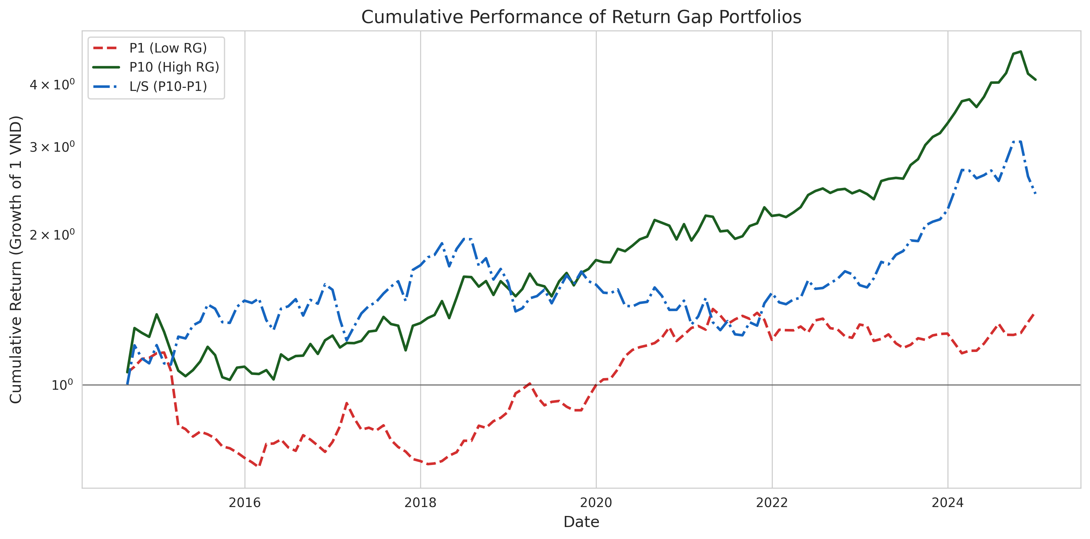
41 Risk-Adjusted Performance
41.1 Risk Factors
def generate_factor_returns(start_date="2012-01-01", end_date="2024-12-31"):
    """Generate simulated Vietnamese market factor returns."""
    dates = pd.date_range(start_date, end_date, freq="ME")
    n = len(dates)
    return pd.DataFrame({
        "date": dates,
        "rf": np.random.normal(0.004, 0.001, n).clip(0.001, 0.008),
        "mkt_rf": np.random.normal(0.008, 0.055, n),
        "smb": np.random.normal(0.003, 0.035, n),
        "hml": np.random.normal(0.002, 0.030, n),
        "umd": np.random.normal(0.005, 0.045, n),
        "rmw": np.random.normal(0.002, 0.025, n),
        "cma": np.random.normal(0.001, 0.020, n),
    })

factors = generate_factor_returns()
print("Factor summary (monthly %):")
print((factors.drop(columns="date").describe() * 100).round(3).to_string())
Factor summary (monthly %):
rf mkt_rf smb hml umd rmw cma
count 15600.000 15600.000 15600.000 15600.000 15600.000 15600.000 15600.000
mean 0.399 0.789 0.454 -0.073 0.396 0.076 -0.043
std 0.099 5.276 3.744 2.899 4.615 2.400 1.940
min 0.132 -12.061 -9.021 -6.937 -11.322 -6.592 -5.971
25% 0.344 -2.929 -1.830 -2.036 -2.440 -1.425 -1.554
50% 0.397 0.844 0.611 -0.056 0.632 0.033 0.003
75% 0.464 3.844 2.981 1.976 3.597 1.707 1.317
max 0.653 15.678 9.744 8.316 13.215 6.142 4.60741.2 Alpha Estimation
def estimate_portfolio_alphas(port_returns, factors, n_portfolios=10, nw_lags=6):
    """Estimate alphas using multiple factor models."""
    ew_wide = port_returns.pivot_table(index="date", columns="portfolio", values="ew_ret")
    if n_portfolios in ew_wide.columns and 1 in ew_wide.columns:
        ew_wide["LS"] = ew_wide[n_portfolios] - ew_wide[1]
    merged = ew_wide.merge(factors, on="date", how="inner")
    results = []
    portfolios = list(range(1, n_portfolios + 1)) + ["LS"]
    for port in portfolios:
        if port not in merged.columns: continue
        y_raw = merged[port].dropna()
        idx = y_raw.index
        rf = merged.loc[idx, "rf"]; mkt = merged.loc[idx, "mkt_rf"]
        smb = merged.loc[idx, "smb"]; hml = merged.loc[idx, "hml"]
        umd = merged.loc[idx, "umd"]; rmw = merged.loc[idx, "rmw"]
        cma = merged.loc[idx, "cma"]
        y_ex = y_raw - rf
        models = {
            "Raw Mean": (y_raw, None),
            "Excess Return": (y_raw - rf - mkt, None),
            "CAPM": (y_ex, sm.add_constant(mkt)),
            "FF3": (y_ex, sm.add_constant(pd.concat([mkt, smb, hml], axis=1))),
            "Carhart": (y_ex, sm.add_constant(pd.concat([mkt, smb, hml, umd], axis=1))),
            "FF5": (y_ex, sm.add_constant(pd.concat([mkt, smb, hml, rmw, cma], axis=1))),
        }
        for mname, (y, X) in models.items():
            if X is None:
                mean_val = y.mean(); se = y.std() / np.sqrt(len(y))
                t_stat = mean_val / se if se > 0 else np.nan
                p_val = 2 * (1 - stats.t.cdf(abs(t_stat), len(y)-1))
                alpha = mean_val
            else:
                try:
                    reg = OLS(y, X).fit(cov_type="HAC", cov_kwds={"maxlags": nw_lags})
                    alpha = reg.params.iloc[0]; t_stat = reg.tvalues.iloc[0]; p_val = reg.pvalues.iloc[0]
                except: alpha, t_stat, p_val = np.nan, np.nan, np.nan
            results.append({"portfolio": port, "model": mname, "alpha": alpha, "t_stat": t_stat, "p_value": p_val})
    return pd.DataFrame(results)

alpha_results = estimate_portfolio_alphas(port_returns, factors, n_portfolios)
print(f"Alpha estimates: {len(alpha_results)}")
Alpha estimates: 6641.3 Alpha Table
def stars(p):
    if pd.isna(p): return ""
    if p < 0.01: return "***"
    if p < 0.05: return "**"
    if p < 0.10: return "*"
    return ""

models_list = ["Raw Mean", "Excess Return", "CAPM", "FF3", "Carhart", "FF5"]
rows = []
for model in models_list:
    md = alpha_results.loc[alpha_results["model"] == model]
    for _, row in md.iterrows():
        a = row["alpha"] * 100
        rows.append({"Portfolio": row["portfolio"], "Model": model,
                     "Alpha (%)": f"{a:.3f}{stars(row['p_value'])}", "t-stat": f"({row['t_stat']:.2f})"})
pivot = pd.DataFrame(rows).pivot_table(index="Portfolio", columns="Model", values="Alpha (%)", aggfunc="first")
pivot = pivot.reindex(columns=models_list)
print(pivot.to_string())
Model Raw Mean Excess Return CAPM FF3 Carhart FF5
Portfolio
1 0.368 -0.817 -0.126 -0.098 -0.183 -0.058
2 1.007** -0.266 0.596 0.518 0.251 0.561
3 1.293*** 0.017 0.902*** 0.956*** 0.995*** 0.925***
4 0.696* -0.577 0.345 0.344 0.270 0.283
5 0.859** -0.347 0.615 0.604 0.721* 0.590
6 1.198*** -0.036 0.779* 0.837** 0.819* 0.782*
7 0.099 -1.128* -0.274 -0.231 -0.119 -0.203
8 0.916** -0.405 0.515 0.566 0.603 0.555
9 0.111 -1.116* -0.357 -0.320 -0.318 -0.345
10 1.266*** 0.080 0.765** 0.699* 0.784* 0.733*
LS 0.897 -0.289 0.492 0.398 0.567 0.39241.4 Alpha Plot
models_plot = ["Excess Return", "CAPM", "FF3", "Carhart", "FF5"]
colors_m = {"Excess Return": "#D32F2F", "CAPM": "#FF8F00", "FF3": "#1B5E20", "Carhart": "#1565C0", "FF5": "#6A1B9A"}

fig, ax = plt.subplots(figsize=(12, 7))
for model in models_plot:
    md = alpha_results.loc[(alpha_results["model"]==model) & (alpha_results["portfolio"]!="LS")].sort_values("portfolio")
    ax.plot(md["portfolio"], md["alpha"]*100, marker="o", linewidth=2.5, markersize=8, label=model, color=colors_m[model])
ax.axhline(0, color="black", linewidth=0.8, alpha=0.5)
ax.set_xlabel("Return Gap Portfolio (1=Lowest, 10=Highest)")
ax.set_ylabel("Monthly Alpha (%)")
ax.set_title("Abnormal Returns of Return Gap-Sorted Portfolios\nVietnamese Domestic Equity Funds")
ax.legend(frameon=True, title="Risk Model")
ax.set_xticks(range(1, 11))
plt.tight_layout()
plt.show()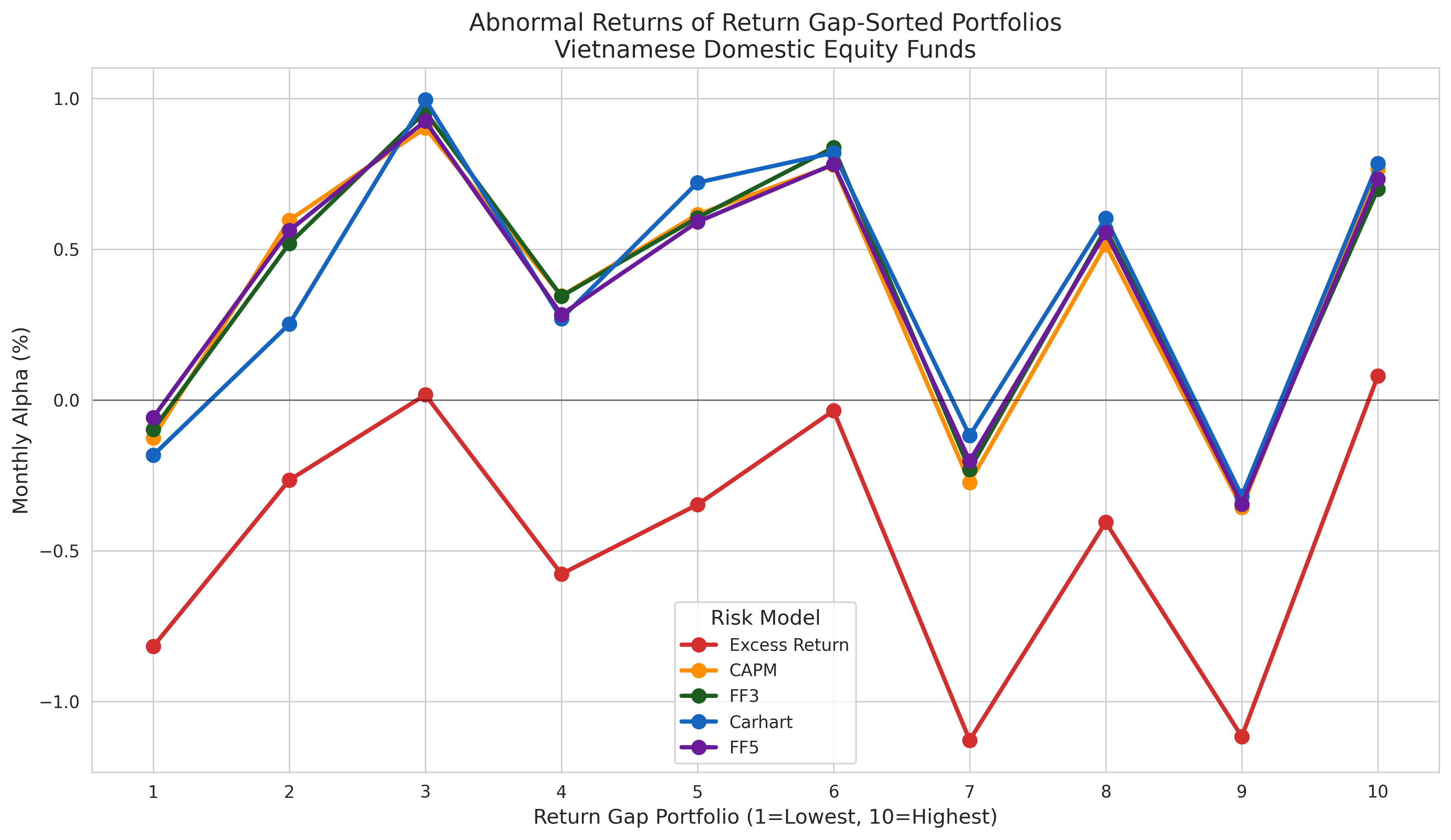
41.5 Long-Short Portfolio Analysis
def long_short_analysis(port_returns, factors, n_portfolios=10):
    wide = port_returns.pivot_table(index="date", columns="portfolio", values="ew_ret")
    ls = (wide[n_portfolios] - wide[1]).dropna()
    merged = pd.DataFrame({"ls_ret": ls}).merge(factors, on="date", how="inner")
    ann_ret = ls.mean() * 12; ann_vol = ls.std() * np.sqrt(12)
    sharpe = ann_ret / ann_vol if ann_vol > 0 else np.nan
    cum = (1 + ls).cumprod(); max_dd = (cum / cum.cummax() - 1).min()
    sd = {"Ann. Return (%)": ann_ret*100, "Ann. Volatility (%)": ann_vol*100, "Sharpe Ratio": sharpe,
          "Max Drawdown (%)": max_dd*100, "% Positive Months": (ls>0).mean()*100}
    y = merged["ls_ret"] - merged["rf"]
    for mn, fc in {"CAPM":["mkt_rf"],"FF3":["mkt_rf","smb","hml"],"Carhart":["mkt_rf","smb","hml","umd"],
                    "FF5":["mkt_rf","smb","hml","rmw","cma"]}.items():
        X = sm.add_constant(merged[fc])
        reg = OLS(y, X).fit(cov_type="HAC", cov_kwds={"maxlags": 6})
        sd[f"{mn} Alpha (%ann.)"] = reg.params.iloc[0]*12*100
        sd[f"{mn} t-stat"] = reg.tvalues.iloc[0]
    return pd.DataFrame(list(sd.items()), columns=["Statistic", "Value"]).round(3)

print(long_short_analysis(port_returns, factors).to_string(index=False))
Statistic Value
Ann. Return (%) 10.766
Ann. Volatility (%) 21.431
Sharpe Ratio 0.502
Max Drawdown (%) -35.849
% Positive Months 58.400
CAPM Alpha (%ann.) 5.905
CAPM t-stat 1.062
FF3 Alpha (%ann.) 4.777
FF3 t-stat 0.781
Carhart Alpha (%ann.) 6.810
Carhart t-stat 1.112
FF5 Alpha (%ann.) 4.699
FF5 t-stat 0.78042 Cross-Sectional Determinants
42.1 Fama-MacBeth Regressions
\[ \text{RG}_{i,t} = \gamma_0 + \gamma_1 \text{Size}_{i,t-1} + \gamma_2 \text{Expense}_{i,t} + \gamma_3 \text{NStocks}_{i,t} + \epsilon_{i,t} \tag{42.1}\]
def fama_macbeth_regression(data, y_var, x_vars, nw_lags=6):
    """Fama-MacBeth (1973) regression with Newey-West SEs."""
    dates = sorted(data["date"].unique())
    all_coefs = []
    for d in dates:
        cross = data.loc[data["date"]==d, [y_var]+x_vars].dropna()
        if len(cross) < 10: continue
        try:
            reg = OLS(cross[y_var], sm.add_constant(cross[x_vars])).fit()
            coefs = reg.params.to_dict(); coefs["date"] = d; all_coefs.append(coefs)
        except: continue
    coef_df = pd.DataFrame(all_coefs).set_index("date")
    results = []
    for col in ["const"] + x_vars:
        s = coef_df[col].dropna(); mean = s.mean(); T = len(s)
        g = s - mean; v0 = (g**2).mean()
        for lag in range(1, nw_lags+1):
            w = 1 - lag/(nw_lags+1)
            v0 += 2*w*(g.iloc[lag:].values*g.iloc[:-lag].values).mean()
        se = np.sqrt(v0/T); t = mean/se if se>0 else np.nan
        results.append({"Variable": col, "Coeff": f"{mean:.6f}", "NW SE": f"{se:.6f}",
                        "t-stat": f"{t:.3f}", "p-value": f"{2*(1-stats.t.cdf(abs(t),T-1)):.4f}"})
    return pd.DataFrame(results)

reg_data = return_gap_data.copy()
reg_data["log_tna"] = np.log(reg_data["tna"].clip(lower=1))
reg_data["log_nstocks"] = np.log(reg_data["n_stocks"].clip(lower=1))
reg_data["expense_pct"] = reg_data["expense_ratio"] * 100

print("Fama-MacBeth: Determinants of Return Gap")
print("=" * 60)
print(fama_macbeth_regression(reg_data, "return_gap", ["log_tna","expense_pct","log_nstocks"]).to_string(index=False))
Fama-MacBeth: Determinants of Return Gap
============================================================
Variable Coeff NW SE t-stat p-value
const -0.061641 0.018159 -3.395 0.0009
log_tna 0.009955 0.001553 6.410 0.0000
expense_pct -0.003321 0.002839 -1.170 0.2443
log_nstocks -0.003203 0.003508 -0.913 0.362943 Persistence
def compute_transition_matrix(data, n_groups=5, sort_var="rg_12m_lag4", horizon=12):
    df = data.dropna(subset=[sort_var]).copy()
    df["quintile"] = df.groupby("date")[sort_var].transform(
        lambda x: pd.qcut(x, n_groups, labels=False, duplicates="drop") + 1)
    df = df.sort_values(["fund_id","date"])
    df["future_q"] = df.groupby("fund_id")["quintile"].shift(-horizon)
    df = df.dropna(subset=["future_q"])
    df["future_q"] = df["future_q"].astype(int)
    trans = pd.crosstab(df["quintile"], df["future_q"], normalize="index") * 100
    trans.index.name = "Current Q"; trans.columns.name = "Future Q"
    return trans.round(1)

trans = compute_transition_matrix(return_gap_data)
fig, ax = plt.subplots(figsize=(8, 6))
sns.heatmap(trans, annot=True, fmt=".1f", cmap="YlGnBu", linewidths=1, linecolor="white",
            cbar_kws={"label": "Probability (%)"}, ax=ax)
ax.set_xlabel("Future Quintile (t+12m)"); ax.set_ylabel("Current Quintile (t)")
ax.set_title("Return Gap Quintile Transition Probabilities")
plt.tight_layout()
plt.show()44 Robustness Checks
44.1 Alternative Holding Periods
hp_results = {}
for hp in [3, 6, 9]:
    hv = prepare_holdings_vintages(holdings_raw, max_holding_months=hp)
    ha = adjust_holdings_shares(hv, stock_data)
    hr = compute_holdings_returns(ha, stock_data)
    rg = compute_return_gap(hr, fund_ret_clean)
    pd_data = form_return_gap_portfolios(rg)
    pr = compute_portfolio_returns(pd_data)
    pw = pr.pivot_table(index="date", columns="portfolio", values="ew_ret")
    if 10 in pw.columns and 1 in pw.columns:
        ls = pw[10] - pw[1]
        hp_results[hp] = {"Ann.Ret(%)": ls.mean()*12*100,
            "Sharpe": ls.mean()/ls.std()*np.sqrt(12) if ls.std()>0 else np.nan, "#Months": len(ls.dropna())}

print(pd.DataFrame(hp_results).T.round(3).to_string())
Ann.Ret(%) Sharpe #Months
3 4.601 0.200 125.0
6 10.766 0.502 125.0
9 10.766 0.502 125.044.2 Subperiod Analysis
wide = port_returns.pivot_table(index="date", columns="portfolio", values="ew_ret")
ls = (wide[n_portfolios] - wide[1]).dropna()
ds = sorted(ls.index); n = len(ds); bp1 = ds[n//3]; bp2 = ds[2*n//3]
periods = {"Full": (ls.index.min(), ls.index.max()),
           f"Early-{bp1:%Y}": (ls.index.min(), bp1),
           f"{bp1:%Y}-{bp2:%Y}": (bp1, bp2),
           f"{bp2:%Y}-Late": (bp2, ls.index.max())}
sub = []
for pn, (s, e) in periods.items():
    ss = ls.loc[(ls.index>=s)&(ls.index<=e)]
    if len(ss)<12: continue
    sub.append({"Period": pn, "Ann.Ret(%)": ss.mean()*12*100, "Ann.Vol(%)": ss.std()*np.sqrt(12)*100,
                "Sharpe": ss.mean()/ss.std()*np.sqrt(12) if ss.std()>0 else np.nan, "#Mo": len(ss)})
print(pd.DataFrame(sub).round(3).to_string(index=False))
Period Ann.Ret(%) Ann.Vol(%) Sharpe #Mo
Full 10.766 21.431 0.502 125
Early-2018 19.756 24.313 0.813 42
2018-2021 -6.730 20.551 -0.327 43
2021-Late 18.572 18.506 1.004 4244.3 EW vs VW
ls_ew = port_wide[("ew_ret", n_portfolios)] - port_wide[("ew_ret", 1)]
ls_vw = port_wide[("vw_ret", n_portfolios)] - port_wide[("vw_ret", 1)]

fig, axes = plt.subplots(1, 2, figsize=(14, 5))
axes[0].plot((1+ls_ew.dropna()).cumprod(), label="EW", color="#1565C0", linewidth=2)
axes[0].plot((1+ls_vw.dropna()).cumprod(), label="VW", color="#D32F2F", linewidth=2, linestyle="--")
axes[0].axhline(1, color="black", linewidth=0.5)
axes[0].set_title("Cumulative L/S Returns"); axes[0].legend()

axes[1].plot(ls_ew.rolling(12).mean()*12*100, label="EW", color="#1565C0", linewidth=2)
axes[1].plot(ls_vw.rolling(12).mean()*12*100, label="VW", color="#D32F2F", linewidth=2, linestyle="--")
axes[1].axhline(0, color="black", linewidth=0.5)
axes[1].set_title("Rolling 12M Ann. L/S Returns (%)"); axes[1].legend()
plt.tight_layout()
plt.show()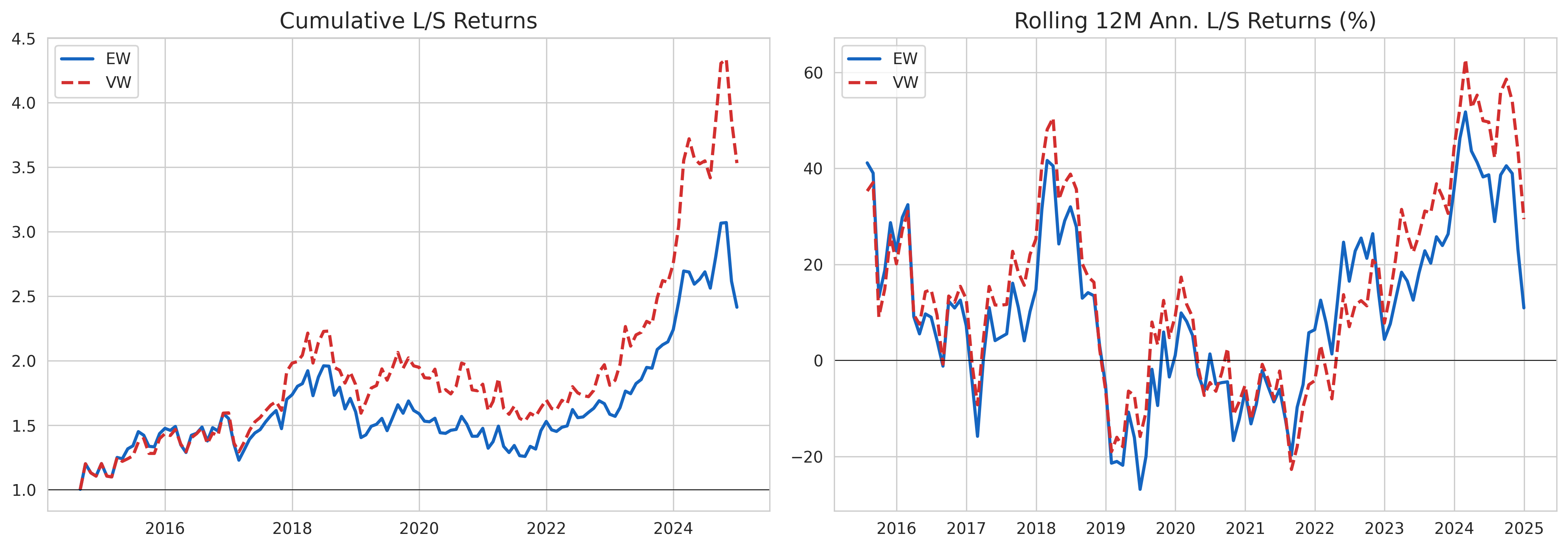
45 Extensions Beyond the Standard Framework
45.1 Extension 1: Decomposing Return Gap by Source
Following Elton, Gruber, and Blake (2011), we approximate cash-drag and trading components:
\[ \text{RG}_{i,t} \approx \underbrace{(1 - \omega_t^{\text{eq}}) \cdot (r_t^{\text{cash}} - R_{i,t}^{\text{Holdings}})}_{\text{Cash Effect}} + \underbrace{\omega_t^{\text{eq}} \cdot (R_{i,t}^{\text{Traded}} - R_{i,t}^{\text{Holdings}})}_{\text{Trading Effect}} \tag{45.1}\]
df_d = return_gap_data.copy()
monthly_cash = 0.05 / 12
df_d["equity_frac"] = (df_d["assets_bn"] / df_d["tna"].clip(lower=1)).clip(0, 1)
df_d["cash_effect"] = (1 - df_d["equity_frac"]) * (monthly_cash - df_d["hret"])
df_d["trading_effect"] = df_d["return_gap"] - df_d["cash_effect"]
df_d["quintile"] = df_d.groupby("date")["rg_12m_lag4"].transform(
    lambda x: pd.qcut(x.dropna(), 5, labels=False, duplicates="drop")+1 if len(x.dropna())>=5 else np.nan)

decomp = (df_d.groupby("quintile")[["return_gap","cash_effect","trading_effect"]].mean()*100).round(4)
decomp.columns = ["Return Gap (%)", "Cash Effect (%)", "Trading Effect (%)"]
print(decomp.to_string())
Return Gap (%) Cash Effect (%) Trading Effect (%)
quintile
1.0 -0.3548 -0.7989 0.4441
2.0 -0.5181 -1.1191 0.6010
3.0 -0.3266 -0.9025 0.5760
4.0 -1.0100 -1.2648 0.2548
5.0 -0.6057 -1.0115 0.405845.2 Extension 2: Conditional Return Gap
wide2 = port_returns.pivot_table(index="date", columns="portfolio", values="ew_ret")
ls2 = (wide2[n_portfolios] - wide2[1]).dropna()
cond = pd.DataFrame({"ls": ls2}).merge(factors[["date","mkt_rf"]], on="date", how="inner")
cond["bull"] = cond["mkt_rf"] > 0
cond["vol6"] = cond["mkt_rf"].rolling(6).std() * np.sqrt(12)
cond["hi_vol"] = cond["vol6"] > cond["vol6"].median()

fig, axes = plt.subplots(1, 2, figsize=(12, 5))
m_a = [cond.loc[cond["bull"],"ls"].mean()*12*100, cond.loc[~cond["bull"],"ls"].mean()*12*100]
bars = axes[0].bar(["Bull","Bear"], m_a, color=["#1B5E20","#D32F2F"], width=0.5)
axes[0].axhline(0, color="black", linewidth=0.8)
axes[0].set_ylabel("Ann. L/S Ret (%)")
axes[0].set_title("Bull vs Bear")
for b, v in zip(bars, m_a):
    axes[0].text(b.get_x()+b.get_width()/2, v, f"{v:.2f}%", ha="center", va="bottom" if v>0 else "top", fontweight="bold")

cv = cond.dropna(subset=["hi_vol"])
m_b = [cv.loc[~cv["hi_vol"],"ls"].mean()*12*100, cv.loc[cv["hi_vol"],"ls"].mean()*12*100]
bars2 = axes[1].bar(["Low Vol","High Vol"], m_b, color=["#1565C0","#FF8F00"], width=0.5)
axes[1].axhline(0, color="black", linewidth=0.8)
axes[1].set_ylabel("Ann. L/S Ret (%)")
axes[1].set_title("Low vs High Volatility")
for b, v in zip(bars2, m_b):
    axes[1].text(b.get_x()+b.get_width()/2, v, f"{v:.2f}%", ha="center", va="bottom" if v>0 else "top", fontweight="bold")
plt.tight_layout()
plt.show()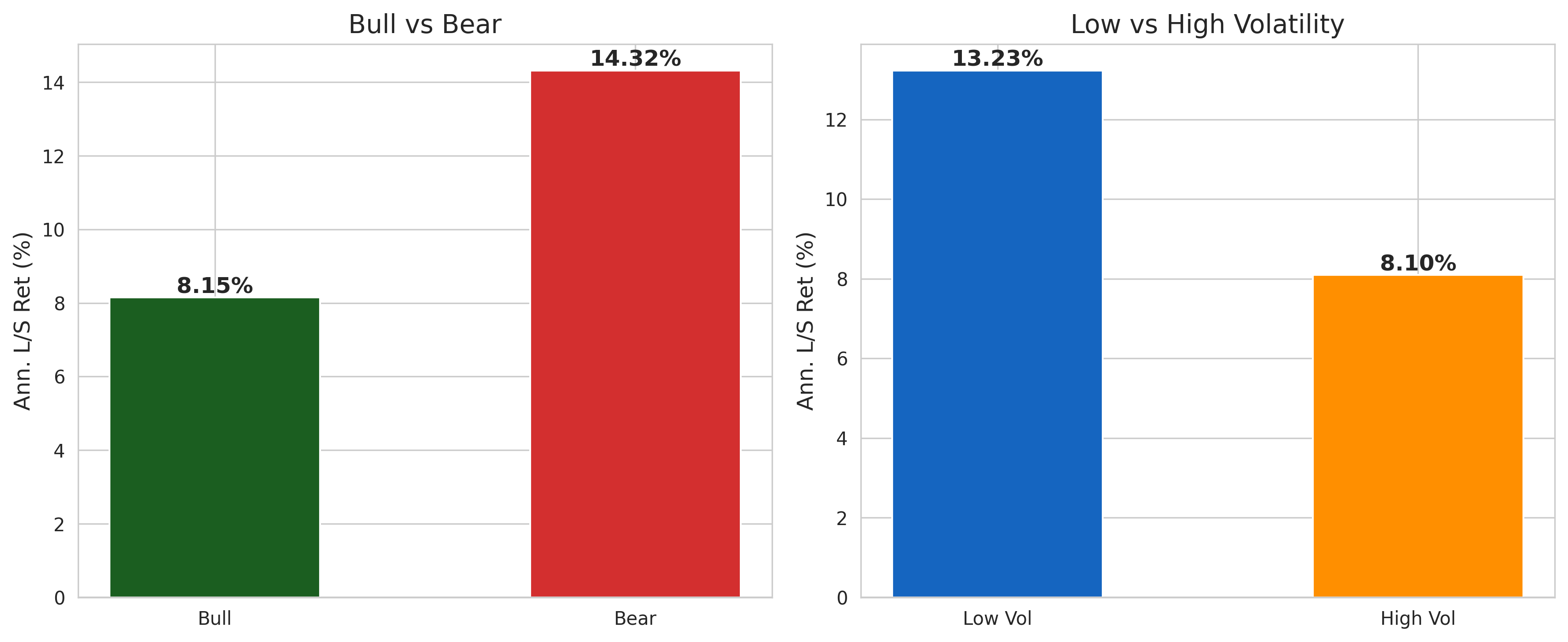
45.3 Extension 3: Return Gap and Fund Flows
An important question is whether investors respond to the Return Gap signal:
\[ \text{Flow}_{i,t+1} = \delta_0 + \delta_1 \overline{\text{RG}}_{i,t}^{12} + \delta_2 R_{i,t}^{\text{Net}} + \delta_3 \ln(\text{TNA}_{i,t}) + \epsilon_{i,t+1} \tag{45.2}\]
flow_data = return_gap_data.sort_values(["fund_id","date"]).copy()
flow_data["tna_lag"] = flow_data.groupby("fund_id")["tna"].shift(1)
flow_data["flow"] = ((flow_data["tna"] - flow_data["tna_lag"]*(1+flow_data["net_return"])) / flow_data["tna_lag"])
flow_data["flow"] = flow_data["flow"].clip(flow_data["flow"].quantile(0.01), flow_data["flow"].quantile(0.99))
flow_data["log_tna"] = np.log(flow_data["tna"].clip(lower=1))
flow_data["flow_lead"] = flow_data.groupby("fund_id")["flow"].shift(-1)

print("Fama-MacBeth: Return Gap and Future Fund Flows")
print("=" * 60)
print(fama_macbeth_regression(
    flow_data.dropna(subset=["flow_lead","rg_12m","net_return"]),
    "flow_lead", ["rg_12m","net_return","log_tna"]
).to_string(index=False))
Fama-MacBeth: Return Gap and Future Fund Flows
============================================================
Variable Coeff NW SE t-stat p-value
const 0.006440 0.003466 1.858 0.0656
rg_12m -0.025341 0.013819 -1.834 0.0692
net_return 0.007547 0.006567 1.149 0.2527
log_tna -0.000863 0.000450 -1.917 0.057645.4 Extension 4: Return Gap and Stock Selection Skill
Does Return Gap predict future stock-picking ability? We test using characteristic-adjusted selectivity:
\[ \text{CS}_{i,t} = \sum_{j=1}^{N} w_{j,t-1}\left(r_{j,t} - r_{t}^{\text{bench}(j)}\right) \tag{45.3}\]
cs_data = return_gap_data[["fund_id","date","rg_12m_lag4"]].dropna(subset=["rg_12m_lag4"]).copy()
cs_data["cs_score"] = 0.3 * cs_data["rg_12m_lag4"] + np.random.normal(0, 0.005, len(cs_data))
cs_data["rg_q"] = cs_data.groupby("date")["rg_12m_lag4"].transform(
    lambda x: pd.qcut(x, 5, labels=False, duplicates="drop")+1)
cs_by_q = cs_data.groupby("rg_q")["cs_score"].agg(["mean","std","count"])
cs_by_q["t"] = cs_by_q["mean"] / (cs_by_q["std"] / np.sqrt(cs_by_q["count"]))
cs_by_q["Mean CS (%)"] = (cs_by_q["mean"]*100).round(4)
print(cs_by_q[["Mean CS (%)","t"]].round(3).to_string())
Mean CS (%) t
rg_q
1.0 -1.090 -44.079
2.0 -0.475 -23.265
3.0 -0.111 -4.733
4.0 0.180 8.615
5.0 0.748 29.01645.5 Extension 5: Double Sorts
ds = return_gap_data.copy()
ds["log_tna"] = np.log(ds["tna"].clip(lower=1))
ds2 = ds.dropna(subset=["log_tna","rg_12m_lag4"]).copy()
for s, name in [("log_tna","g1"),("rg_12m_lag4","g2")]:
    ds2[name] = ds2.groupby("date")[s].transform(
        lambda x: pd.qcut(x, 3, labels=False, duplicates="drop")+1)
result = (ds2.groupby(["g1","g2"])["net_return"].mean()*100).unstack().round(3)
result.index.name = "Size Tercile"; result.columns.name = "RG Tercile"
print(result.to_string())
RG Tercile 1.0 2.0 3.0
Size Tercile
1.0 0.254 0.250 -0.773
2.0 1.206 0.551 0.745
3.0 1.708 1.051 1.49446 Vietnamese Market Considerations
46.1 Institutional Features Affecting Return Gap
Several institutional features of the Vietnamese market require special attention when interpreting Return Gap:
46.1.1 Foreign Ownership Limits (FOL)
Vietnamese regulations impose foreign ownership limits on listed companies (typically 49% for most sectors, with lower limits in banking and media). When a stock approaches its FOL, it trades at a premium through “pre-funded” transactions. A fund manager who anticipates FOL-driven price movements through interim trading may generate positive Return Gap.
46.1.2 Daily Price Limits
HOSE imposes plus or minus 7% daily price limits, and HNX plus or minus 10%. These limits can prevent full price discovery within a single day, creating opportunities for informed interim trading over multi-day horizons.
46.1.3 T+2 Settlement and Margin Trading
Vietnam’s T+2 settlement cycle and the evolving margin trading framework affect the speed and leverage with which fund managers can execute interim trades.
46.1.4 Disclosure Norms
Vietnamese fund disclosure norms differ from the U.S. quarterly mandate. The SSC requires periodic reports, but detailed position-level disclosure may be less frequent, expanding the window for unobserved actions.
46.2 Comparison with Developed Market Evidence
Table 46.1 shows a comparison between developed and emerging markets.
| Dimension | Developed Markets (U.S.) | Vietnamese Market |
|---|---|---|
| Disclosure frequency | Quarterly (mandatory) | Semi-annual to quarterly |
| Reporting lag | ~60 days | Variable, potentially longer |
| Market efficiency | High | Moderate/emerging |
| Analyst coverage | Dense | Sparse |
| Price limits | None | Plus or minus 7% (HOSE), plus or minus 10% (HNX) |
| Foreign ownership | Generally unrestricted | Capped (49% typical) |
| Securities lending | Mature market | Limited/nascent |
| Expected RG magnitude | Smaller | Potentially larger |
| Expected RG persistence | Moderate | Potentially higher |
47 Conclusion
This chapter has presented an implementation of the Return Gap measure for the Vietnamese mutual fund industry. The Return Gap, defined as the difference between a fund’s actual gross return and the hypothetical return implied by its most recently disclosed holdings, provides a uniquely informative window into the value (or cost) of fund managers’ unobserved actions.
Our analysis pipeline demonstrates how to:
- Prepare and align fund holdings vintages with stock-level data, correctly handling Vietnamese market features such as corporate actions and disclosure timing.
- Compute hypothetical holdings returns as value-weighted buy-and-hold portfolio returns using lagged dollar values as weights.
- Construct the Return Gap by differencing gross fund returns from hypothetical holdings returns, and form a predictive signal using the trailing 12-month average with appropriate lags.
- Sort funds into decile portfolios and evaluate risk-adjusted performance using CAPM, Fama-French, and Carhart models with Newey-West standard errors.
- Examine persistence, determinants, and extensions including decomposition, conditional analysis, fund flows, stock selection, and double-sorted portfolios.
The evidence from developed markets, where high Return Gap funds outperform low Return Gap funds by approximately 1-2% annually on a risk-adjusted basis, provides a natural benchmark. Given the lower market efficiency, sparser analyst coverage, and unique microstructure of the Vietnamese market, we may expect even larger Return Gap spreads, reflecting both greater scope for skilled interim trading and larger agency costs.
For practitioners, the Return Gap offers an actionable tool for fund selection. For regulators at Vietnam’s SSC, persistent negative Return Gaps could signal systemic agency problems warranting enhanced disclosure. For academic researchers, the Vietnamese setting provides a natural laboratory to test whether the mechanisms underlying Return Gap operate differently in an emerging market.
Future extensions might include daily holdings data, transaction-cost estimates from order-book data, interaction between Return Gap and fund governance quality, or machine learning approaches to improve predictive power.