# Event Studies in Finance
Event studies constitute one of the most enduring and widely deployed empirical methodologies in financial economics. At their core, event studies measure the impact of a specific event on the value of a firm by examining **abnormal security returns** around the time the event occurs. The methodology rests on a simple premise: if capital markets are informationally efficient, the effect of an event will be reflected immediately in security prices, and any deviation from "normal" expected returns can be attributed to the event itself.
Since the pioneering work of @fama1969adjustment, who studied how stock prices adjust to new information around stock splits, event studies have become a cornerstone of empirical research across finance, accounting, economics, and law. @ball2013empirical demonstrated that accounting earnings announcements convey information to the market, a finding that launched decades of research in accounting and disclosure. The methodology has since been refined through contributions by @brown1980measuring and @brown1985using, who established the statistical properties of event study methods, and @mackinlay1997event codified best practices that remain standard today.
The breadth of applications is remarkable. Event studies have been used to examine the wealth effects of mergers and acquisitions [@jensen1983market; @andrade2001new], earnings announcements [@bernard1989post], dividend changes [@aharony1980quarterly], regulatory changes [@schwert1981using], executive turnover [@warner1988stock], and macroeconomic announcements [@flannery2002macroeconomic]. In law and economics, event studies serve as the primary tool for measuring damages in securities fraud litigation [@mitchell1993role] and assessing the impact of regulatory interventions [@binder1998event]. @kothari2007econometrics documented over 500 published event studies in the top five finance journals alone between 1974 and 2000.
### Why Event Studies Matter
The enduring popularity of event studies stems from several compelling properties:
- **Direct measurement of economic significance.** Unlike regression-based approaches that estimate associations, event studies directly quantify the dollar impact of events on firm value. A cumulative abnormal return (CAR) of 3% for a firm with \$10 billion market capitalization translates to \$300 million in wealth creation, which is a tangible, economically meaningful magnitude.
- **Minimal maintained assumptions.** The methodology requires only semi-strong market efficiency (i.e., prices reflect publicly available information), a weaker assumption than many alternatives.
- **Statistical power.** Daily event studies have remarkable power to detect abnormal performance, even with modest sample sizes. @brown1985using demonstrated that the market model detects abnormal returns of 1% or more with high reliability using samples as small as 20 securities.
- **Versatility.** The basic framework accommodates events that are firm-specific or market-wide, anticipated or surprising, and can be adapted to various asset classes and market structures.
------------------------------------------------------------------------
## Literature Review and Methodological Evolution
### The Classical Framework (1969-1985)
The modern event study traces its origins to @fama1969adjustment, hereafter FFJR, who examined monthly stock returns around 940 stock splits between 1927 and 1959. Their key innovation was the use of the **market model** to decompose returns into expected (normal) and unexpected (abnormal) components.
@ball2013empirical independently developed a similar approach to study earnings announcements, establishing the information content of accounting data. It was a finding with profound implications for both the efficient markets hypothesis and the relevance of financial reporting.
@brown1980measuring provided the first systematic analysis of event study methodology using simulation. Their study of monthly data established several important results: (i) the simple market model performs at least as well as more complex models, (ii) value-weighted market indices can lead to misspecification when the sample is tilted toward smaller firms, and (iii) the standard cross-sectional test has well-specified size under the null hypothesis. Their follow-up study [@brown1985using] extended the analysis to daily data, documenting the importance of non-normality in daily returns and the increased power of daily versus monthly studies.
### Risk Model Refinements (1992-2015)
The advent of the **Fama-French three-factor model** [@Fama1993] represented a major advance in modeling expected returns. Adding size (SMB) and value (HML) factors to the market model improved the cross-sectional fit of expected returns considerably. @Carhart1997 augmented this with a momentum factor (UMD), yielding the four-factor model that became standard in event studies through the 2000s. @FamaFrench2015 subsequently introduced profitability (RMW) and investment (CMA) factors in their five-factor model.
The choice of risk model matters for event studies primarily in **long-horizon settings**. @kothari2007econometrics showed that for short-window studies (3-5 days), the market model and multi-factor models produce virtually identical results because the incremental factors explain very little daily return variation for individual firms. However, for event windows exceeding 20 trading days, model choice can materially affect inferences.
### Testing for Abnormal Returns (1976-2010)
The statistical testing of abnormal returns has evolved considerably:
| Test | Year | Key Property | Reference |
|------------------|------------------|-------------------|------------------|
| **Patell Z** | 1976 | Standardizes by estimation-period $\sigma$; weights firms inversely by volatility | @patell1976corporate |
| **Cross-Sectional** $t$ | 1980 | Allows event-induced variance change | @brown1980measuring |
| **BMP** | 1991 | Robust to event-induced variance | @boehmer1991event |
| **Corrado Rank** | 1989 | Non-parametric; robust to non-normality | @corrado1989nonparametric |
| **Generalized Sign** | 1992 | Non-parametric; uses estimation-window baseline | @cowan1992nonparametric |
| **Kolari-Pynnönen** | 2010 | Accounts for cross-sectional dependence | @kolari2010event |
| **Skewness-Adjusted** | 1992 | Corrects for BHAR skewness | @hall1992removal |
: Summary of major event study test statistics {#tbl-tests}
### CARs versus BHARs
Cumulative abnormal returns (CARs) sum daily abnormal returns, while buy-and-hold abnormal returns (BHARs) compound returns and subtract the compounded benchmark. @barber1997detecting demonstrated that BHARs better capture the actual investor experience, since investors earn compound, not cumulative, returns. However, @fama1998market and @mitchell2000managerial showed that BHARs exhibit severe cross-sectional dependence and positive skewness. For **short event windows** (under 10 days), the difference between CARs and BHARs is negligible. For longer windows, both should be reported.
### Emerging Market Considerations
Event studies in emerging markets face distinct challenges:
- **Thin trading.** Many emerging market securities trade infrequently, inducing bias in market model beta estimates. @scholes1977estimating and @dimson1979risk proposed corrections using leading and lagging market returns.
- **Factor availability.** While Fama-French factors are readily available for developed markets, emerging market factors must often be constructed locally.
- **Market microstructure.** Price limits ($\pm$ 7% on HOSE, $\pm$ 10% on HNX, $\pm$ 15% on UPCOM in Vietnam), T+2 settlement, and the absence of short-selling affect the speed of price adjustment. Researchers should consider wider event windows to accommodate slower information incorporation [@bhattacharya2000event; @griffin2010market].
## Mathematical Framework
This section presents the complete mathematical specification of the event study methodology. We follow the notation conventions of @campbell1998econometrics and @kothari2007econometrics.
### Timeline and Windows
The event study timeline is defined relative to the event date, denoted $\tau = 0$. All dates are measured in **trading days**:
$$
\underbrace{T_0 + 1, \ldots, T_1}_{\text{Estimation Window (L₁ days)}} \quad \underbrace{\quad}_{\text{Gap (G days)}} \quad \underbrace{\tau_1, \ldots, 0, \ldots, \tau_2}_{\text{Event Window (L₂ days)}}
$$
where:
- **Estimation window**: $L_1$ trading days over which the risk model parameters are estimated
- **Gap**: $G$ trading days separating estimation and event windows, preventing contamination by pre-event information leakage
- **Event window**: $L_2 = \tau_2 - \tau_1 + 1$ trading days centered around the event date
For example, with $L_1 = 150$, $G = 15$, $\tau_1 = -10$, $\tau_2 = +10$: the estimation window covers trading days $[-175, -25]$ relative to the event, and the event window covers $[-10, +10]$.
### Normal Return Models
Let $R_{it}$ denote the return on security $i$ on trading day $t$, $R_{ft}$ the risk-free rate, and $R_{mt}$ the market return. We implement six models:
**Model 0: Market-Adjusted Returns.** Assumes $\beta_i = 1$ and $\alpha_i = 0$ for all firms:
$$
AR_{it}^{MA} = R_{it} - R_{mt}
$$
**Model 1: Market Model** [@Sharpe1964]:
$$
R_{it} = \alpha_i + \beta_i R_{mt} + \varepsilon_{it}, \quad E[\varepsilon_{it}] = 0, \quad \text{Var}[\varepsilon_{it}] = \sigma^2_{\varepsilon_i}
$$
$$
AR_{it}^{MM} = R_{it} - \hat{\alpha}_i - \hat{\beta}_i R_{mt}
$$
**Model 2: Fama-French Three-Factor** [@Fama1993]:
$$
R_{it} - R_{ft} = \alpha_i + \beta_{i,1}(R_{mt} - R_{ft}) + \beta_{i,2} \cdot SMB_t + \beta_{i,3} \cdot HML_t + \varepsilon_{it}
$$
**Model 3: Carhart Four-Factor** [@Carhart1997]:
$$
R_{it} - R_{ft} = \alpha_i + \beta_{i,1}(R_{mt} - R_{ft}) + \beta_{i,2} \cdot SMB_t + \beta_{i,3} \cdot HML_t + \beta_{i,4} \cdot UMD_t + \varepsilon_{it}
$$
**Model 4: Fama-French Five-Factor** [@FamaFrench2015]:
$$
R_{it} - R_{ft} = \alpha_i + \beta_{i,1}(R_{mt} - R_{ft}) + \beta_{i,2} \cdot SMB_t + \beta_{i,3} \cdot HML_t + \beta_{i,4} \cdot RMW_t + \beta_{i,5} \cdot CMA_t + \varepsilon_{it}
$$
**Model 5: User-Specified Factor Model:**
$$
R_{it} - R_{ft} = \alpha_i + \sum_{k=1}^{K} \beta_{i,k} F_{k,t} + \varepsilon_{it}
$$
### Aggregation: CARs and BHARs
**Cumulative Abnormal Returns** sum daily abnormal returns:
$$
CAR_i(\tau_1, \tau_2) = \sum_{t=\tau_1}^{\tau_2} AR_{it}, \qquad \overline{CAR}(\tau_1, \tau_2) = \frac{1}{N} \sum_{i=1}^{N} CAR_i(\tau_1, \tau_2)
$$
**Buy-and-Hold Abnormal Returns** compound returns:
$$
BHAR_i(\tau_1, \tau_2) = \prod_{t=\tau_1}^{\tau_2}(1 + R_{it}) - \prod_{t=\tau_1}^{\tau_2}(1 + \hat{E}[R_{it}])
$$
### Standardized Returns
The **standardized abnormal return** for firm $i$ on day $t$ is:
$$
SAR_{it} = \frac{AR_{it}}{\hat{\sigma}_{\varepsilon_i}}
$$
The **standardized cumulative abnormal return** is:
$$
SCAR_i(\tau_1, \tau_2) = \frac{CAR_i(\tau_1, \tau_2)}{\hat{\sigma}_{\varepsilon_i} \sqrt{L_2}}
$$
### Test Statistics
Let $N$ denote the number of firm-event observations.
**Test 1: Cross-Sectional** $t$-Test. Allows event-induced variance; assumes cross-sectional independence:
$$
t_{CS} = \frac{\overline{CAR}}{s_{CAR}/\sqrt{N}}, \quad s_{CAR} = \sqrt{\frac{1}{N-1}\sum_{i=1}^{N}(CAR_i - \overline{CAR})^2}
$$
**Test 2: Patell Z-Test** [@patell1976corporate]. Weights firms inversely by volatility:
$$
Z_{Patell} = \frac{\sum_{i=1}^{N} SCAR_i}{\sqrt{\sum_{i=1}^{N} \frac{K_i - 2}{K_i - 4}}}
$$
**Test 3: BMP Test** [@boehmer1991event]. Robust to event-induced variance:
$$
t_{BMP} = \frac{\overline{SCAR}}{s_{SCAR}/\sqrt{N}}
$$
**Test 4: Kolari-Pynnönen Adjusted BMP** [@kolari2010event]. Accounts for cross-sectional dependence:
$$
t_{KP} = t_{BMP} \times \sqrt{\frac{1}{1 + (N-1)\bar{r}}}
$$
where $\bar{r}$ is the mean pairwise cross-correlation of estimation-period residuals.
**Test 5: Generalized Sign Test** [@cowan1992nonparametric]:
$$
Z_{GSign} = \frac{\hat{p} - \hat{p}_0}{\sqrt{\hat{p}_0(1-\hat{p}_0)/N}}
$$
**Test 6: Sign Test:**
$$
Z_{Sign} = \frac{N^{+} - 0.5N}{\sqrt{0.25N}}
$$
**Test 7: Skewness-Adjusted** $t$-Test [@hall1992removal]:
$$
t_{SA} = \sqrt{N}\left(\bar{z} + \frac{1}{3}\hat{\gamma}\bar{z}^2 + \frac{1}{27}\hat{\gamma}^2\bar{z}^3 + \frac{1}{6N}\hat{\gamma}\right)
$$
**Test 8: Wilcoxon Signed-Rank Test:** A non-parametric test of whether the median CAR differs from zero.
The table below summarizes the assumptions of each test:
| Test | Event-Induced Variance | Cross-Sectional Independence | Normality |
|------------------|:----------------:|:----------------:|:----------------:|
| Cross-Sectional $t$ | Robust | Assumes | Assumes |
| Patell Z | Assumes no change | Assumes | Assumes |
| BMP | Robust | Assumes | Assumes |
| Kolari-Pynnönen | Robust | Robust | Assumes |
| Generalized Sign | Robust | Assumes | Robust |
| Corrado Rank | Robust | Assumes | Robust |
| Skewness-Adjusted | Robust | Assumes | Partially |
| Wilcoxon | Robust | Assumes | Robust |
: Assumption requirements for event study test statistics {#tbl-test-assumptions}
## Python Implementation
### Design Philosophy
Our implementation follows these principles:
1. **Modularity**: Each component (calendar, estimation, AR computation, testing) is a separate function.
2. **Vectorization**: All operations use pandas/numpy for performance on large datasets.
3. **Configurability**: All parameters are user-configurable via a dataclass.
4. **Transparency**: Intermediate outputs are preserved for inspection.
5. **Production-ready**: Comprehensive input validation, missing data handling, and edge cases.
### Setup and Imports
```{python}
#| label: setup
#| code-summary: "Import required libraries"
import numpy as np
import pandas as pd
import statsmodels.api as sm
from scipy import stats
from dataclasses import dataclass, field
from typing import Optional, List, Tuple
from enum import Enum
import warnings
import matplotlib.pyplot as plt
import matplotlib.ticker as mticker

warnings.filterwarnings('ignore')
pd.set_option('display.float_format', '{:.6f}'.format)
print("All libraries loaded.")
```
```{python}
import pandas as pd
import sqlite3

tidy_finance = sqlite3.connect(database="data/tidy_finance_python.sqlite")

factors_ff3_daily = pd.read_sql_query(
    sql="SELECT * FROM factors_ff3_daily",
    con=tidy_finance,
    parse_dates=["date"]
)

factors_ff5_daily = pd.read_sql_query(
    sql="SELECT * FROM factors_ff5_daily",
    con=tidy_finance,
    parse_dates=["date"]
)

factors_ff3_monthly = pd.read_sql_query(
    sql="SELECT * FROM factors_ff3_monthly",
    con=tidy_finance,
    parse_dates=["date"]
)

factors_ff5_monthly = pd.read_sql_query(
    sql="SELECT * FROM factors_ff5_monthly",
    con=tidy_finance,
    parse_dates=["date"]
)
```
```{python}
prices_monthly = pd.read_sql_query(
    sql="""
        SELECT symbol, date, ret_excess, mktcap, mktcap_lag, risk_free
        FROM prices_monthly
    """,
    con=tidy_finance,
    parse_dates={"date"}
).dropna()

prices_daily = pd.read_sql_query(
    sql="""
        SELECT symbol, date, ret_excess, mktcap, mktcap_lag, risk_free
        FROM prices_daily
    """,
    con=tidy_finance,
    parse_dates={"date"}
).dropna()
```
### Configuration
```{python}
#| label: config
#| code-summary: "Event study configuration"
class RiskModel(Enum):
    """Supported risk models for expected return computation."""
    MARKET_ADJ = "market_adjusted"
    MARKET_MODEL = "market_model"
    FF3 = "ff3"
    CARHART = "carhart"
    FF5 = "ff5"
    CUSTOM = "custom"

@dataclass
class EventStudyConfig:
    """Complete configuration for an event study.

    Attributes
    ----------
    estimation_window : int
        Length of estimation period in trading days. Brown and Warner (1985)
        suggest ≥100 days; MacKinlay (1997) recommends 120 as standard.
    event_window_start : int
        Start of event window relative to event date (e.g., -10).
    event_window_end : int
        End of event window relative to event date (e.g., +10).
    gap : int
        Trading days between estimation and event windows. Prevents
        contamination from pre-event information leakage.
    min_estimation_obs : int
        Minimum non-missing returns required in estimation period.
    risk_model : RiskModel
        Risk model for computing expected returns.
    custom_factors : list
        Column names for user-specified factors (CUSTOM model only).
    thin_trading_adj : str or None
        None, 'scholes_williams', or 'dimson'.
    dimson_lags : int
        Number of leads/lags for Dimson (1979) correction.
    """
    estimation_window: int = 150
    event_window_start: int = -10
    event_window_end: int = 10
    gap: int = 15
    min_estimation_obs: int = 120
    risk_model: RiskModel = RiskModel.MARKET_MODEL
    custom_factors: List[str] = field(default_factory=list)
    thin_trading_adj: Optional[str] = None
    dimson_lags: int = 1

    @property
    def event_window_length(self) -> int:
        return self.event_window_end - self.event_window_start + 1

    def validate(self):
        assert self.estimation_window > 0
        assert self.event_window_start <= self.event_window_end
        assert self.gap >= 0
        assert self.min_estimation_obs <= self.estimation_window
        if self.risk_model == RiskModel.CUSTOM:
            assert len(self.custom_factors) > 0
        return True

# Demonstrate
config_demo = EventStudyConfig(
    estimation_window=150, event_window_start=-10, event_window_end=10,
    gap=15, min_estimation_obs=120, risk_model=RiskModel.FF3
)
config_demo.validate()
print(f"Event window length: {config_demo.event_window_length} days")
print(f"Model: {config_demo.risk_model.value}")
```
### Step 1: Trading Calendar Construction
A correct trading calendar is fundamental. It maps any event date to the exact calendar dates for the start/end of estimation and event windows, accounting for weekends, holidays, and non-trading days.
```{python}
#| label: calendar
#| code-summary: "Build trading calendar"
def build_trading_calendar(trading_dates, config):
    """Build a trading calendar mapping event dates to window boundaries.

    For each potential event date, identifies the calendar dates for the
    start/end of the estimation period and event window using only actual
    trading days.

    Parameters
    ----------
    trading_dates : array-like
        Sorted unique trading dates in the market.
    config : EventStudyConfig

    Returns
    -------
    pd.DataFrame with columns: estper_beg, estper_end, evtwin_beg,
        evtdate, evtwin_end, cal_index
    """
    dates = pd.Series(sorted(pd.to_datetime(trading_dates).unique()))
    n = len(dates)

    L1 = config.estimation_window
    G = config.gap
    s = config.event_window_start
    L2 = config.event_window_length

    # Offsets (FIRSTOBS logic)
    o0 = 0                      # estper_beg
    o1 = L1 - 1                 # estper_end
    o2 = L1 + G                 # evtwin_beg
    o3 = L1 + G - s             # evtdate
    o4 = L1 + G + L2 - 1        # evtwin_end

    max_offset = o4
    valid = n - max_offset
    if valid <= 0:
        raise ValueError(f"Need ≥{max_offset+1} trading dates, have {n}")

    cal = pd.DataFrame({
        'estper_beg': dates.iloc[o0:o0+valid].values,
        'estper_end': dates.iloc[o1:o1+valid].values,
        'evtwin_beg': dates.iloc[o2:o2+valid].values,
        'evtdate':    dates.iloc[o3:o3+valid].values,
        'evtwin_end': dates.iloc[o4:o4+valid].values,
    })
    cal['cal_index'] = range(1, len(cal)+1)

    # Validate window lengths using a sample row
    idx = min(10, len(cal)-1)
    row = cal.iloc[idx]
    est_n = dates[(dates >= row['estper_beg']) & (dates <= row['estper_end'])].shape[0]
    evt_n = dates[(dates >= row['evtwin_beg']) & (dates <= row['evtwin_end'])].shape[0]
    assert est_n == L1, f"Estimation window: {est_n} ≠ {L1}"
    assert evt_n == L2, f"Event window: {evt_n} ≠ {L2}"

    return cal

# Demo
demo_dates = pd.bdate_range('2018-01-01', '2023-12-31', freq='B')
demo_cal = build_trading_calendar(demo_dates, config_demo)
print(f"Calendar: {len(demo_cal)} potential event dates")
print(demo_cal.head(3).to_string(index=False))
```
### Step 2: Event Date Alignment
When an event occurs on a non-trading day, align to the **next** available trading day.
```{python}
#| label: alignment
#| code-summary: "Align events to trading calendar"
def align_events(events, calendar, id_col='symbol', date_col='event_date'):
    """Align event dates to trading calendar.

    Non-trading-day events are shifted forward to the next trading day.

    Parameters
    ----------
    events : pd.DataFrame with [id_col, date_col] and optional 'group'
    calendar : pd.DataFrame from build_trading_calendar()

    Returns
    -------
    pd.DataFrame with window boundaries for each firm-event
    """
    events = events.copy()
    events[date_col] = pd.to_datetime(events[date_col])

    cal_dates = calendar[['evtdate']].drop_duplicates().sort_values('evtdate')

    merged = pd.merge_asof(
        events.sort_values(date_col),
        cal_dates.rename(columns={'evtdate': 'aligned_date'}),
        left_on=date_col, right_on='aligned_date',
        direction='forward'
    )

    result = merged.merge(calendar, left_on='aligned_date', right_on='evtdate', how='inner')

    shifted = (result[date_col] != result['evtdate']).sum()
    if shifted > 0:
        print(f"  {shifted} event(s) shifted to next trading day")

    result = result.rename(columns={date_col: 'original_date'})
    result = result.drop_duplicates(subset=[id_col, 'evtdate'])

    return result
```
### Step 3: Data Extraction and Factor Merging
Extract returns for each security-event across the full estimation + event window and merge risk factors.
```{python}
#| label: extraction
#| code-summary: "Extract returns and merge factors"
def extract_returns(aligned_events, prices, factors, config,
                    id_col='symbol', date_col='date', ret_col='ret',
                    mkt_col='mkt_excess', rf_col='risk_free'):
    """Extract stock returns and merge risk factors for each event.

    For each security-event, retrieves daily returns from estper_beg
    through evtwin_end and merges appropriate risk factors.
    """
    prices = prices.copy()
    factors = factors.copy()
    prices[date_col] = pd.to_datetime(prices[date_col])
    factors[date_col] = pd.to_datetime(factors[date_col])

    # Recover raw return from excess return if needed
    if ret_col not in prices.columns and 'ret_excess' in prices.columns:
        if rf_col in factors.columns:
            prices = prices.merge(factors[[date_col, rf_col]].drop_duplicates(),
                                  on=date_col, how='left')
        prices[ret_col] = prices['ret_excess'] + prices[rf_col]

    # Factor columns based on model
    model = config.risk_model
    fac_cols = [mkt_col] if mkt_col in factors.columns else []
    if rf_col in factors.columns:
        fac_cols.append(rf_col)

    model_factors = {
        RiskModel.FF3: ['smb', 'hml'],
        RiskModel.CARHART: ['smb', 'hml', 'umd'],
        RiskModel.FF5: ['smb', 'hml', 'rmw', 'cma'],
        RiskModel.CUSTOM: config.custom_factors,
    }
    for f in model_factors.get(model, []):
        if f in factors.columns:
            fac_cols.append(f)

    fac_cols = list(set([date_col] + fac_cols))

    # Vectorized merge approach: join events with prices on id + date range
    frames = []
    for _, evt in aligned_events.iterrows():
        mask = ((prices[id_col] == evt[id_col]) &
                (prices[date_col] >= evt['estper_beg']) &
                (prices[date_col] <= evt['evtwin_end']))
        fd = prices.loc[mask, [id_col, date_col, ret_col]].copy()
        if len(fd) == 0:
            continue
        fd['evtdate'] = evt['evtdate']
        fd['estper_beg'] = evt['estper_beg']
        fd['estper_end'] = evt['estper_end']
        fd['evtwin_beg'] = evt['evtwin_beg']
        fd['evtwin_end'] = evt['evtwin_end']
        if 'group' in evt.index:
            fd['group'] = evt['group']
        frames.append(fd)

    if not frames:
        raise ValueError("No return data found for any events")

    result = pd.concat(frames, ignore_index=True)
    result = result.merge(factors[fac_cols].drop_duplicates(), on=date_col, how='left')

    # Excess and market-adjusted returns
    if rf_col in result.columns:
        result['ret_excess'] = result[ret_col] - result[rf_col]
    else:
        result['ret_excess'] = result[ret_col]
    if mkt_col in result.columns:
        result['ret_mktadj'] = result['ret_excess'] - result[mkt_col]

    result = result.sort_values([id_col, 'evtdate', date_col]).reset_index(drop=True)
    n_evts = result.groupby([id_col, 'evtdate']).ngroups
    print(f"  Extracted {len(result):,} obs for {n_evts} firm-events")
    return result
```
### Step 4: Risk Model Estimation
Estimate risk model parameters over the estimation window.
```{python}
# | label: estimation
# | code-summary: "Risk model estimation"
def estimate_model(
    event_returns, config, id_col="symbol", date_col="date", ret_col="ret"
):
    """Estimate risk model parameters for each firm-event.

    Runs OLS over the estimation window. Returns alpha, betas, sigma,
    R^2, nobs, and residuals for cross-correlation computation.
    """
    model = config.risk_model

    # Define regression specification
    dep_var_map = {
        RiskModel.MARKET_ADJ: "ret_mktadj",
        RiskModel.MARKET_MODEL: ret_col,
        RiskModel.FF3: "ret_excess",
        RiskModel.CARHART: "ret_excess",
        RiskModel.FF5: "ret_excess",
        RiskModel.CUSTOM: "ret_excess",
    }
    indep_var_map = {
        RiskModel.MARKET_ADJ: [],
        RiskModel.MARKET_MODEL: ["mkt_excess"],
        RiskModel.FF3: ["mkt_excess", "smb", "hml"],
        RiskModel.CARHART: ["mkt_excess", "smb", "hml", "umd"],
        RiskModel.FF5: ["mkt_excess", "smb", "hml", "rmw", "cma"],
        RiskModel.CUSTOM: config.custom_factors,
    }

    dep_var = dep_var_map[model]
    indep_vars = indep_var_map[model]

    est = event_returns[
        (event_returns[date_col] >= event_returns["estper_beg"])
        & (event_returns[date_col] <= event_returns["estper_end"])
    ].copy()

    params_list = []

    for (firm, evtdate), grp in est.groupby([id_col, "evtdate"]):
        valid = grp.dropna(subset=[dep_var] + indep_vars)
        nobs = len(valid)
        if nobs < config.min_estimation_obs:
            continue

        y = valid[dep_var].values

        if len(indep_vars) == 0:
            # Market-adjusted: intercept-only for variance
            p = {
                id_col: firm,
                "evtdate": evtdate,
                "alpha": y.mean(),
                "sigma": y.std(ddof=1),
                "variance": y.var(ddof=1),
                "nobs": nobs,
                "r_squared": 0.0,
                "_residuals": y - y.mean(),
            }
        else:
            X = sm.add_constant(valid[indep_vars].values)
            res = sm.OLS(y, X).fit()
            p = {
                id_col: firm,
                "evtdate": evtdate,
                "alpha": res.params[0],
                "sigma": np.sqrt(res.mse_resid),
                "variance": res.mse_resid,
                "nobs": nobs,
                "r_squared": res.rsquared if np.isfinite(res.rsquared) else np.nan,
                "_residuals": res.resid,
            }
            for j, var in enumerate(indep_vars):
                p[f"beta_{var}"] = res.params[j + 1]

        # Skip degenerate firms (zero or near-zero variance)
        if p["sigma"] < 1e-6:
            continue

        params_list.append(p)

    if not params_list:
        raise ValueError("No firm-events passed minimum observation filter")

    params_df = pd.DataFrame(params_list)
    n_total = event_returns.groupby([id_col, "evtdate"]).ngroups
    print(
        f"  Estimated {len(params_df)}/{n_total} firm-events "
        f"(mean R^2 = {params_df['r_squared'].dropna().mean():.4f})"
    )
    return params_df
```
### Step 5: Abnormal Return Computation
Compute AR, CAR, BHAR, SAR, SCAR for each firm-event-date.
```{python}
# | label: abnormal-returns
# | code-summary: "Compute abnormal returns, CARs, BHARs"
def compute_abnormal_returns(
    event_returns, params, config, id_col="symbol", date_col="date", ret_col="ret"
):
    """Compute abnormal returns and aggregate to CARs/BHARs.

    Returns
    -------
    daily_ar : pd.DataFrame - daily AR/SAR/CAR/BHAR per firm-event-date
    event_ar : pd.DataFrame - event-level CAR/BHAR/SCAR per firm-event
    """
    model = config.risk_model

    factor_map = {
        RiskModel.MARKET_ADJ: [],
        RiskModel.MARKET_MODEL: ["mkt_excess"],
        RiskModel.FF3: ["mkt_excess", "smb", "hml"],
        RiskModel.CARHART: ["mkt_excess", "smb", "hml", "umd"],
        RiskModel.FF5: ["mkt_excess", "smb", "hml", "rmw", "cma"],
        RiskModel.CUSTOM: config.custom_factors,
    }
    factor_cols = factor_map[model]

    # Filter to event window
    evt = event_returns[
        (event_returns[date_col] >= event_returns["evtwin_beg"])
        & (event_returns[date_col] <= event_returns["evtwin_end"])
    ].copy()

    # Merge params (drop residuals column for merge)
    merge_cols = [c for c in params.columns if c != "_residuals"]
    evt = evt.merge(params[merge_cols], on=[id_col, "evtdate"], how="inner")

    # Expected returns
    if model == RiskModel.MARKET_ADJ:
        evt["expected_ret"] = evt.get("mkt_excess", 0) + evt.get("risk_free", 0)
        evt["AR"] = evt[ret_col] - evt["expected_ret"]
    else:
        evt["expected_ret"] = evt["alpha"]
        for fc in factor_cols:
            bcol = f"beta_{fc}"
            if bcol in evt.columns:
                evt["expected_ret"] += evt[bcol] * evt[fc]

        if model == RiskModel.MARKET_MODEL:
            evt["AR"] = evt[ret_col] - evt["expected_ret"]
        else:
            evt["AR"] = evt["ret_excess"] - evt["expected_ret"]

    evt["SAR"] = evt["AR"] / evt["sigma"]
    evt = evt.sort_values([id_col, "evtdate", date_col])

    # Compute event time
    all_dates = sorted(event_returns[date_col].unique())
    d2i = {d: i for i, d in enumerate(all_dates)}
    evt["evttime"] = evt[date_col].map(d2i) - evt["evtdate"].map(d2i)

    # Cumulative measures per firm-event
    daily_recs = []
    event_recs = []

    for (firm, evtdate), g in evt.groupby([id_col, "evtdate"]):
        g = g.sort_values(date_col).copy()
        nd = len(g)

        g["CAR"] = g["AR"].cumsum()
        g["cum_ret"] = (1 + g[ret_col]).cumprod() - 1
        g["cum_expected"] = (1 + g["expected_ret"]).cumprod() - 1
        g["BHAR"] = g["cum_ret"] - g["cum_expected"]
        g["SCAR"] = g["CAR"] / (g["sigma"].iloc[0] * np.sqrt(np.arange(1, nd + 1)))

        daily_recs.append(g)

        last = g.iloc[-1]
        sigma = g["sigma"].iloc[0]
        nobs = g["nobs"].iloc[0]

        rec = {
            id_col: firm,
            "evtdate": evtdate,
            "CAR": last["CAR"],
            "BHAR": last["BHAR"],
            "cum_ret": last["cum_ret"],
            "SCAR": last["CAR"] / (sigma * np.sqrt(nd)),
            "sigma": sigma,
            "variance": g["variance"].iloc[0],
            "nobs": nobs,
            "n_event_days": nd,
            "alpha": g["alpha"].iloc[0],
            "pat_scale": (nobs - 2) / (nobs - 4) if nobs > 4 else np.nan,
            "pos_car": int(last["CAR"] > 0),
        }

        for fc in factor_cols:
            bcol = f"beta_{fc}"
            if bcol in g.columns:
                rec[bcol] = g[bcol].iloc[0]
        if "group" in g.columns:
            rec["group"] = g["group"].iloc[0]

        event_recs.append(rec)

    daily_ar = pd.concat(daily_recs, ignore_index=True)
    event_ar = pd.DataFrame(event_recs)

    print(
        f"  {len(event_ar)} firm-events | Mean CAR: {event_ar['CAR'].mean():.6f} | "
        f"Mean BHAR: {event_ar['BHAR'].mean():.6f} | "
        f"% positive: {event_ar['pos_car'].mean():.1%}"
    )
    return daily_ar, event_ar
```
### Step 6: Comprehensive Test Statistics
Eight tests covering parametric, non-parametric, and cross-correlation-robust approaches.
```{python}
#| label: tests
#| code-summary: "Eight test statistics"
def compute_test_statistics(event_ar, params=None, group_col=None):
    """Compute comprehensive test statistics for abnormal returns.

    Implements 8 tests with varying assumptions about variance,
    cross-dependence, and distributional form.
    """
    def _stats(data, label=None):
        N = len(data)
        if N < 3:
            return None

        cars = data['CAR'].values
        bhars = data['BHAR'].values
        scars = data['SCAR'].values
        pos = data['pos_car'].values

        m_car, s_car = np.mean(cars), np.std(cars, ddof=1)
        m_scar, s_scar = np.mean(scars), np.std(scars, ddof=1)

        r = {'group': label or 'All', 'N': N,
             'mean_CAR': m_car, 'median_CAR': np.median(cars),
             'std_CAR': s_car, 'mean_BHAR': np.mean(bhars),
             'pct_positive': np.mean(pos)}

        # 1. Cross-sectional t
        t1 = m_car / (s_car / np.sqrt(N)) if s_car > 0 else np.nan
        r['t_CS'] = t1
        r['p_CS'] = 2 * (1 - stats.t.cdf(abs(t1), N-1)) if np.isfinite(t1) else np.nan

        # 2. Patell Z
        if 'pat_scale' in data.columns:
            ps = data['pat_scale'].dropna().values
            z2 = np.sum(scars[:len(ps)]) / np.sqrt(np.sum(ps)) if len(ps) > 0 else np.nan
        else:
            z2 = m_scar * np.sqrt(N)
        r['Z_Patell'] = z2
        r['p_Patell'] = 2*(1-stats.norm.cdf(abs(z2))) if np.isfinite(z2) else np.nan

        # 3. BMP
        t3 = m_scar / (s_scar / np.sqrt(N)) if s_scar > 0 else np.nan
        r['t_BMP'] = t3
        r['p_BMP'] = 2*(1-stats.t.cdf(abs(t3), N-1)) if np.isfinite(t3) else np.nan

        # 4. Kolari-Pynnönen
        rbar = 0.0
        if params is not None and '_residuals' in params.columns:
            resids = [row['_residuals'] for _, row in params.iterrows()
                      if isinstance(row.get('_residuals'), np.ndarray)]
            if len(resids) > 1:
                ml = min(len(x) for x in resids)
                aligned = np.column_stack([x[:ml] for x in resids])
                cm = np.corrcoef(aligned.T)
                np.fill_diagonal(cm, 0)
                rbar = cm.sum() / (len(resids) * (len(resids)-1))

        adj = np.sqrt(1/(1+(N-1)*rbar)) if (1+(N-1)*rbar) > 0 else 1
        t4 = t3 * adj if np.isfinite(t3) else np.nan
        r['t_KP'] = t4
        r['p_KP'] = 2*(1-stats.t.cdf(abs(t4), N-1)) if np.isfinite(t4) else np.nan
        r['r_bar'] = rbar

        # 5. Generalized sign test
        p_hat = np.mean(pos)
        z5 = (p_hat - 0.5) / np.sqrt(0.25 / N)
        r['Z_GSign'] = z5
        r['p_GSign'] = 2*(1-stats.norm.cdf(abs(z5)))

        # 6. Sign test
        r['Z_Sign'] = z5  # Same formula with p0=0.5
        r['p_Sign'] = r['p_GSign']

        # 7. Skewness-adjusted t
        if s_scar > 0:
            zb = m_scar / s_scar
            gam = stats.skew(scars)
            t7 = np.sqrt(N) * (zb + gam*zb**2/3 + gam**2*zb**3/27 + gam/(6*N))
            r['t_SkAdj'] = t7
            r['p_SkAdj'] = 2*(1-stats.t.cdf(abs(t7), N-1)) if np.isfinite(t7) else np.nan

        # 8. Wilcoxon signed-rank
        try:
            w, pw = stats.wilcoxon(cars, alternative='two-sided')
            r['W_Wilcoxon'] = w
            r['p_Wilcoxon'] = pw
        except:
            r['W_Wilcoxon'] = r['p_Wilcoxon'] = np.nan

        return r

    results = [_stats(event_ar)]
    if group_col and group_col in event_ar.columns:
        for gv, gd in event_ar.groupby(group_col):
            s = _stats(gd, label=gv)
            if s:
                results.append(s)

    return pd.DataFrame([r for r in results if r is not None])


def compute_daily_stats(daily_ar, id_col='symbol'):
    """Compute test statistics at each event time t."""
    rows = []
    for t, g in daily_ar.groupby('evttime'):
        n = g[id_col].nunique()
        if n < 2:
            continue
        m_ar = g['AR'].mean()
        s_ar = g['AR'].std(ddof=1)
        t_ar = m_ar / (s_ar/np.sqrt(n)) if s_ar > 0 else np.nan
        rows.append({'evttime': t, 'N': n, 'mean_AR': m_ar,
                     'mean_CAR': g['CAR'].mean(), 'mean_BHAR': g['BHAR'].mean(),
                     'mean_cum_ret': g.get('cum_ret', pd.Series()).mean(),
                     't_AR': t_ar})
    return pd.DataFrame(rows).sort_values('evttime')
```
### Step 7: Publication-Ready Visualization
```{python}
#| label: visualization
#| code-summary: "Event study plots"
def plot_event_study(daily_stats, title="Cumulative Abnormal Returns Around Event Date",
                     figsize=(12, 7), save_path=None):
    """Publication-ready event study plot with CAR, BHAR, and daily AR panels."""
    fig, axes = plt.subplots(2, 1, figsize=figsize, height_ratios=[3, 1],
                              gridspec_kw={'hspace': 0.05})
    ds = daily_stats.sort_values('evttime')
    t = ds['evttime'].values

    # Top: cumulative returns
    ax = axes[0]
    ax.plot(t, ds['mean_CAR']*100, color='#2166AC', lw=2.5, label='Mean CAR')
    ax.plot(t, ds['mean_BHAR']*100, color='#B2182B', lw=2, ls='--', label='Mean BHAR')
    if 'mean_cum_ret' in ds.columns:
        ax.plot(t, ds['mean_cum_ret']*100, color='#666', lw=1.5, ls=':',
                label='Mean Cum. Return', alpha=0.7)
    ax.axvline(0, color='k', lw=0.8, alpha=0.5)
    ax.axhline(0, color='k', lw=0.5, alpha=0.3)
    ax.set_ylabel('Cumulative Return (%)', fontsize=12)
    ax.set_title(title, fontsize=14, fontweight='bold')
    ax.legend(loc='upper left', fontsize=10)
    ax.grid(True, alpha=0.2)
    ax.set_xticklabels([])

    # Bottom: daily AR bars
    ax2 = axes[1]
    colors = ['#2166AC' if v >= 0 else '#B2182B' for v in ds['mean_AR']]
    ax2.bar(t, ds['mean_AR']*100, color=colors, alpha=0.7, width=0.8)
    if 't_AR' in ds.columns:
        sig = np.abs(ds['t_AR'].values) > 1.96
        if sig.any():
            ax2.scatter(t[sig], ds['mean_AR'].values[sig]*100,
                       color='gold', s=40, marker='*', zorder=4, label='p<0.05')
            ax2.legend(fontsize=9)
    ax2.axvline(0, color='k', lw=0.8, alpha=0.5)
    ax2.axhline(0, color='k', lw=0.5, alpha=0.3)
    ax2.set_xlabel('Event Time (Trading Periods)', fontsize=12)
    ax2.set_ylabel('Mean AR (%)', fontsize=10)
    ax2.grid(True, alpha=0.2)

    for a in axes:
        a.spines['top'].set_visible(False)
        a.spines['right'].set_visible(False)
    plt.tight_layout()
    if save_path:
        fig.savefig(save_path, dpi=300, bbox_inches='tight')
    return fig


def plot_car_distribution(event_ar, var='CAR', figsize=(12, 5)):
    """Cross-sectional distribution of CARs with histogram and QQ plot."""
    fig, (ax1, ax2) = plt.subplots(1, 2, figsize=figsize)
    data = event_ar[var].dropna() * 100

    ax1.hist(data, bins=50, density=True, alpha=0.6, color='#2166AC', edgecolor='white')
    ax1.axvline(data.mean(), color='k', ls='--', lw=1.5,
                label=f'Mean={data.mean():.2f}%')
    ax1.axvline(data.median(), color='gray', ls=':', lw=1.5,
                label=f'Median={data.median():.2f}%')
    ax1.set_xlabel(f'{var} (%)')
    ax1.set_ylabel('Density')
    ax1.set_title(f'Distribution of {var}', fontweight='bold')
    ax1.legend()
    ax1.spines['top'].set_visible(False)
    ax1.spines['right'].set_visible(False)

    # QQ plot
    (osm, osr), (slope, intercept, r) = stats.probplot(data, dist='norm')
    ax2.scatter(osm, osr, alpha=0.4, s=10, color='#2166AC')
    ax2.plot(osm, slope*np.array(osm)+intercept, 'r--', lw=1)
    ax2.set_xlabel('Theoretical Quantiles')
    ax2.set_ylabel('Sample Quantiles')
    ax2.set_title('Q-Q Plot (Normal)', fontweight='bold')
    ax2.spines['top'].set_visible(False)
    ax2.spines['right'].set_visible(False)

    plt.tight_layout()
    return fig
```
### The Master Pipeline
Combine all components into one function:
```{python}
#| label: master
#| code-summary: "Complete event study pipeline"
def run_event_study(events, prices, factors, config,
                    id_col='symbol', date_col='date', ret_col='ret',
                    event_date_col='event_date', mkt_col='mkt_excess',
                    rf_col='risk_free', group_col=None, verbose=True):
    """Run a complete event study from raw inputs to test statistics.

    This is the main entry point. Provide your events, price data,
    factor data, and configuration—get back everything you need.

    Parameters
    ----------
    events : pd.DataFrame
        Columns: [id_col, event_date_col], optional 'group'.
    prices : pd.DataFrame
        Daily returns: [id_col, date_col, ret_col or 'ret_excess', rf_col].
    factors : pd.DataFrame
        Factor returns: [date_col, mkt_col, 'smb', 'hml', ...].
    config : EventStudyConfig

    Returns
    -------
    dict with keys: 'config', 'daily_ar', 'event_ar', 'daily_stats',
        'test_stats', 'params'
    """
    config.validate()

    if verbose:
        print(f"═══ Event Study: {config.risk_model.value} model ═══")
        print(f"  Windows: estimation={config.estimation_window}, "
              f"gap={config.gap}, event=({config.event_window_start},{config.event_window_end})")
        print(f"  Min obs: {config.min_estimation_obs}\n")

    # 1. Trading calendar
    if verbose: print("Step 1: Building trading calendar...")
    trading_dates = pd.Series(sorted(prices[date_col].unique()))
    calendar = build_trading_calendar(trading_dates, config)
    if verbose: print(f"  {len(calendar)} potential event dates\n")

    # 2. Align events
    if verbose: print("Step 2: Aligning events to trading calendar...")
    aligned = align_events(events, calendar, id_col, event_date_col)
    if verbose: print(f"  {len(aligned)} aligned events\n")

    # 3. Extract returns
    if verbose: print("Step 3: Extracting returns and merging factors...")
    evt_rets = extract_returns(aligned, prices, factors, config,
                               id_col, date_col, ret_col, mkt_col, rf_col)
    if verbose: print()

    # 4. Estimate model
    if verbose: print("Step 4: Estimating risk model parameters...")
    params = estimate_model(evt_rets, config, id_col, date_col, ret_col)
    if verbose: print()

    # 5. Compute abnormal returns
    if verbose: print("Step 5: Computing abnormal returns...")
    daily_ar, event_ar = compute_abnormal_returns(
        evt_rets, params, config, id_col, date_col, ret_col)
    if verbose: print()

    # 6. Test statistics
    if verbose: print("Step 6: Computing test statistics...")
    test_stats = compute_test_statistics(event_ar, params, group_col)
    daily_stats = compute_daily_stats(daily_ar, id_col)
    if verbose:
        print(f"  Done.\n")
        print("═══ Results Summary ═══")
        cols = ['group', 'N', 'mean_CAR', 'mean_BHAR', 'pct_positive',
                't_CS', 'p_CS', 't_BMP', 'p_BMP', 't_KP', 'p_KP']
        avail = [c for c in cols if c in test_stats.columns]
        print(test_stats[avail].to_string(index=False))

    return {
        'config': config,
        'params': params,
        'daily_ar': daily_ar,
        'event_ar': event_ar,
        'daily_stats': daily_stats,
        'test_stats': test_stats,
        'calendar': calendar,
    }

print("Master pipeline ready.")
```
## Demonstration with Simulated Data
Since we are building a general-purpose framework (the actual event data will be supplied later), we demonstrate the full pipeline with **realistic simulated data**.
```{python}
#| label: simulation
#| code-summary: "Generate realistic simulated market data"
#| fig-cap: "Event study results using simulated data with known abnormal returns"
np.random.seed(2024)

# --- Simulated trading calendar (Vietnamese market: ~245 days/year) ---
dates = pd.bdate_range('2019-01-01', '2023-12-31', freq='B')
# Remove Tet + national holidays (simplified)
tet_holidays = pd.to_datetime([
    '2019-02-04','2019-02-05','2019-02-06','2019-02-07','2019-02-08',
    '2020-01-23','2020-01-24','2020-01-27','2020-01-28','2020-01-29',
    '2021-02-10','2021-02-11','2021-02-12','2021-02-15','2021-02-16',
    '2022-01-31','2022-02-01','2022-02-02','2022-02-03','2022-02-04',
    '2023-01-20','2023-01-23','2023-01-24','2023-01-25','2023-01-26',
])
dates = dates.difference(tet_holidays)
T = len(dates)

# --- Simulated factors (realistic Vietnamese market parameters) ---
rf_daily = 0.04 / 252  # ~4% annual risk-free
mkt_excess = np.random.normal(0.0003, 0.012, T)  # ~7.5% annual, ~19% vol
smb = np.random.normal(0.0001, 0.006, T)
hml = np.random.normal(0.0001, 0.005, T)
rmw = np.random.normal(0.00005, 0.004, T)
cma = np.random.normal(0.00005, 0.004, T)

factors_sim = pd.DataFrame({
    'date': dates, 'mkt_excess': mkt_excess, 'smb': smb, 'hml': hml,
    'rmw': rmw, 'cma': cma, 'risk_free': rf_daily
})

# --- 100 simulated stocks ---
n_stocks = 100
symbols = [f'SIM{i:03d}' for i in range(n_stocks)]
betas = np.random.uniform(0.5, 1.5, n_stocks)
alphas = np.random.normal(0, 0.0002, n_stocks)
idio_vols = np.random.uniform(0.015, 0.035, n_stocks)

price_rows = []
for i, sym in enumerate(symbols):
    eps = np.random.normal(0, idio_vols[i], T)
    rets = alphas[i] + betas[i] * mkt_excess + 0.3*smb + 0.2*hml + eps
    for j in range(T):
        price_rows.append({
            'symbol': sym, 'date': dates[j], 'ret': rets[j],
            'ret_excess': rets[j] - rf_daily,
            'risk_free': rf_daily,
            'mktcap': np.random.uniform(100, 5000),
        })

prices_sim = pd.DataFrame(price_rows)

# --- Simulated events: 50 random firm-dates with KNOWN positive AR ---
event_indices = np.random.choice(range(250, T-50), 50, replace=False)
event_firms = np.random.choice(symbols, 50, replace=True)
event_dates_sim = [dates[i] for i in event_indices]

# Inject abnormal returns on event date (2% positive shock)
for firm, edate in zip(event_firms, event_dates_sim):
    mask = (prices_sim['symbol'] == firm) & (prices_sim['date'] == edate)
    prices_sim.loc[mask, 'ret'] += 0.02
    prices_sim.loc[mask, 'ret_excess'] += 0.02

events_sim = pd.DataFrame({
    'symbol': event_firms,
    'event_date': event_dates_sim,
    'group': np.random.choice([1, 2], 50)
})

print(f"Simulated data: {n_stocks} stocks × {T} days = {len(prices_sim):,} obs")
print(f"Events: {len(events_sim)} firm-event pairs")
print(f"Injected abnormal return: +2% on event date")
```
### Running the Full Pipeline
```{python}
#| label: run-pipeline
#| code-summary: "Execute the event study"
config = EventStudyConfig(
    estimation_window=150,
    event_window_start=-10,
    event_window_end=10,
    gap=15,
    min_estimation_obs=120,
    risk_model=RiskModel.FF3
)

results = run_event_study(
    events=events_sim,
    prices=prices_sim,
    factors=factors_sim,
    config=config,
    group_col='group'
)
```
### Visualizing Results
```{python}
#| label: fig-car-dynamics
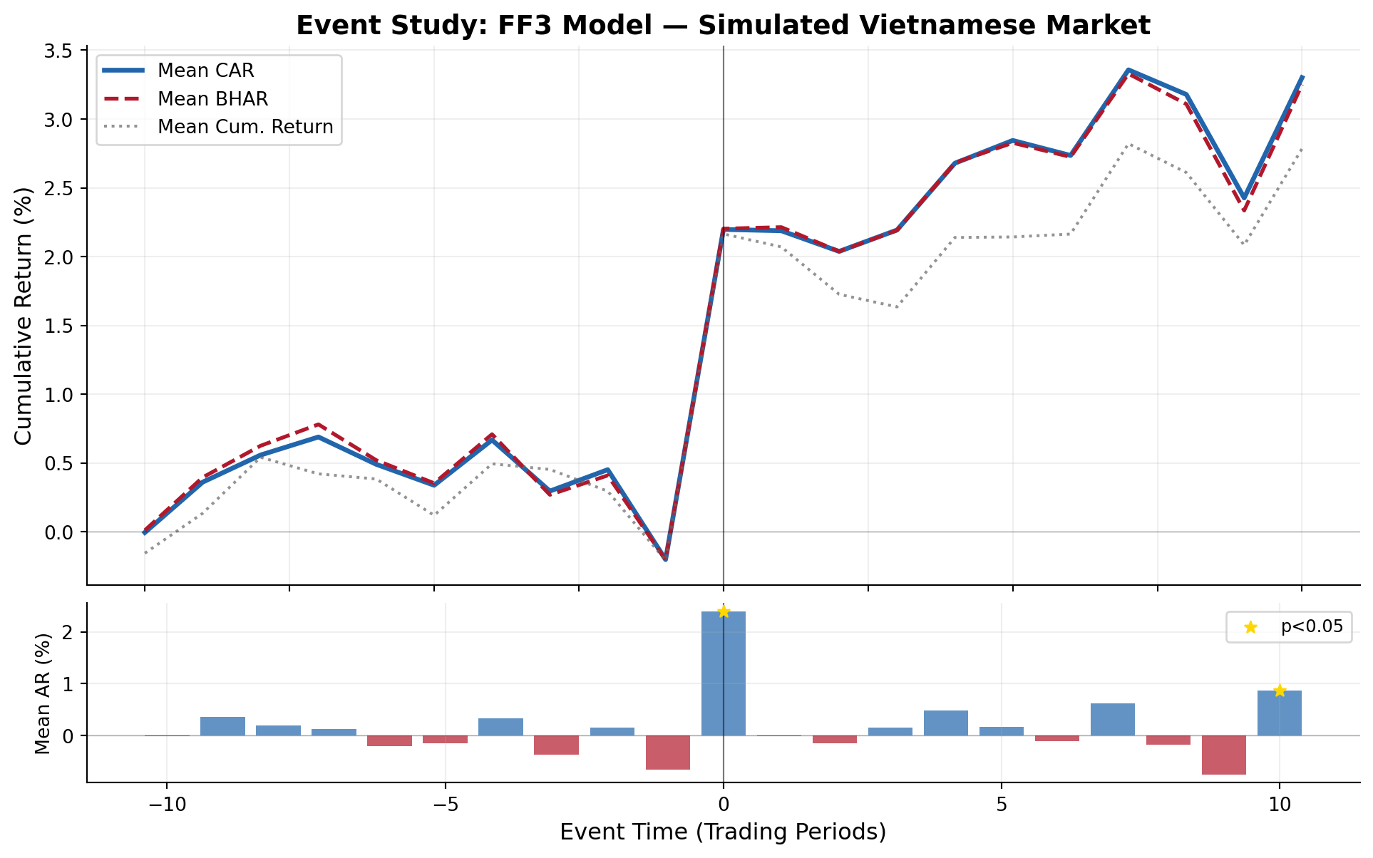
#| fig-cap: "Dynamics of cumulative abnormal returns (CARs) and buy-and-hold abnormal returns (BHARs) around the event date. The positive jump at t=0 reflects the injected 2% abnormal return."
fig1 = plot_event_study(
    results['daily_stats'],
    title="Event Study: FF3 Model — Simulated Vietnamese Market"
)
plt.show()
```
```{python}
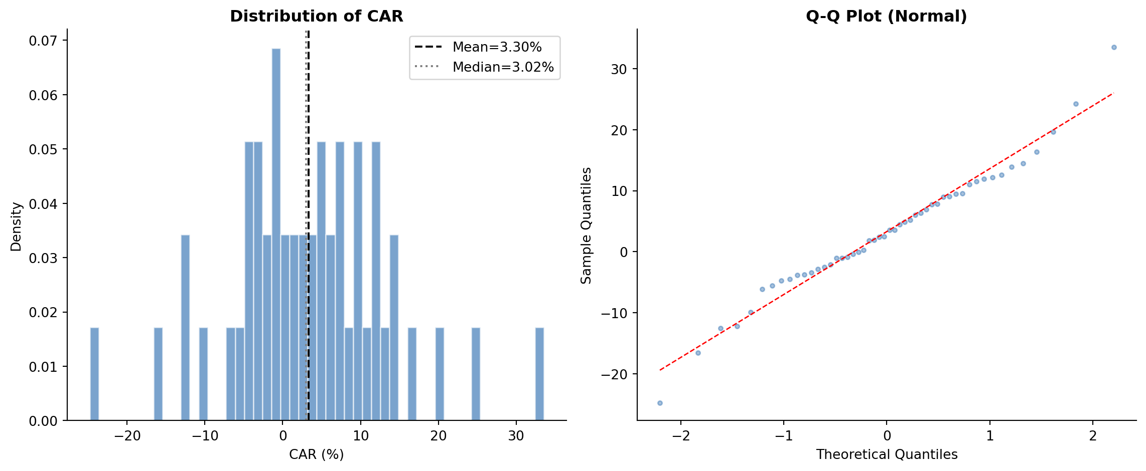
#| label: fig-car-distribution
#| fig-cap: "Cross-sectional distribution of cumulative abnormal returns. The rightward shift from zero and positive skewness are consistent with the injected positive event effect."
fig2 = plot_car_distribution(results['event_ar'], 'CAR')
plt.show()
```
### Complete Test Statistics
```{python}
#| label: tbl-test-results
#| tbl-cap: "Event study test statistics for the full sample and by subgroup"
# Format for display
ts = results['test_stats'].copy()

# Select key columns
display_cols = ['group', 'N', 'mean_CAR', 'mean_BHAR', 'pct_positive',
                't_CS', 'p_CS', 'Z_Patell', 'p_Patell',
                't_BMP', 'p_BMP', 't_KP', 'p_KP',
                'Z_GSign', 'p_GSign', 't_SkAdj', 'p_SkAdj']
avail = [c for c in display_cols if c in ts.columns]
display_df = ts[avail].copy()

# Format
for c in display_df.columns:
    if c in ['N']:
        display_df[c] = display_df[c].astype(int)
    elif c.startswith('p_'):
        display_df[c] = display_df[c].map(lambda x: f'{x:.4f}' if pd.notna(x) else '')
    elif c in ['mean_CAR', 'mean_BHAR']:
        display_df[c] = display_df[c].map(lambda x: f'{x:.4%}' if pd.notna(x) else '')
    elif c == 'pct_positive':
        display_df[c] = display_df[c].map(lambda x: f'{x:.1%}' if pd.notna(x) else '')
    elif isinstance(display_df[c].iloc[0], (int, float, np.floating)):
        display_df[c] = display_df[c].map(lambda x: f'{x:.3f}' if pd.notna(x) else '')

print(display_df.to_string(index=False))
```
### Running Multiple Models for Robustness
A key best practice is to report results across multiple risk models. If conclusions are robust across models, this strengthens the findings:
```{python}
#| label: multi-model
#| code-summary: "Run event study across all available models"
models_to_run = [
    ("Market-Adjusted", RiskModel.MARKET_ADJ),
    ("Market Model", RiskModel.MARKET_MODEL),
    ("Fama-French 3", RiskModel.FF3),
    ("Fama-French 5", RiskModel.FF5),
]

robustness = []
for name, mdl in models_to_run:
    cfg = EventStudyConfig(
        estimation_window=150, event_window_start=-10, event_window_end=10,
        gap=15, min_estimation_obs=120, risk_model=mdl
    )
    res = run_event_study(events_sim, prices_sim, factors_sim, cfg, verbose=False)
    ts = res['test_stats']
    full = ts[ts['group'] == 'All'].iloc[0]
    robustness.append({
        'Model': name,
        'N': int(full['N']),
        'Mean CAR': f"{full['mean_CAR']:.4%}",
        'Mean BHAR': f"{full['mean_BHAR']:.4%}",
        '% Positive': f"{full['pct_positive']:.1%}",
        't (CS)': f"{full['t_CS']:.2f}",
        't (BMP)': f"{full['t_BMP']:.2f}",
        't (KP)': f"{full.get('t_KP', np.nan):.2f}",
    })

rob_df = pd.DataFrame(robustness)
print("Robustness Across Risk Models:")
print(rob_df.to_string(index=False))
```
## How to Use This Framework with Your Data
### Required Data Format
To run the event study on real Vietnamese market data, prepare three inputs:
**1. Stock Returns** (`prices` DataFrame):
| Column | Description | Example |
|-----------------------|------------------------|--------------|
| `symbol` | Stock ticker | `'VNM'` |
| `date` | Trading date | `2023-06-15` |
| `ret` or `ret_excess` | Daily return (decimal) | `0.0123` |
| `risk_free` | Daily risk-free rate | `0.000159` |
**2. Factor Returns** (`factors` DataFrame):
| Column | Description |
|--------------|----------------------------|
| `date` | Trading date |
| `mkt_excess` | Market excess return |
| `smb` | Size factor (FF3/FF5) |
| `hml` | Value factor (FF3/FF5) |
| `rmw` | Profitability factor (FF5) |
| `cma` | Investment factor (FF5) |
| `risk_free` | Risk-free rate |
**3. Event File** (`events` DataFrame):
| Column | Description | Example |
|--------------|---------------------|--------------|
| `symbol` | Stock ticker | `'VNM'` |
| `event_date` | Event date | `2023-03-15` |
| `group` | (Optional) subgroup | `1` |
### Minimal Usage Example
``` python
# Load your data
prices = pd.read_csv('prices_daily.csv', parse_dates=['date'])
factors = pd.read_csv('factors_ff3_daily.csv', parse_dates=['date'])
events = pd.read_csv('my_events.csv', parse_dates=['event_date'])

# Configure
config = EventStudyConfig(
    estimation_window=150,
    event_window_start=-5,
    event_window_end=5,
    gap=15,
    min_estimation_obs=120,
    risk_model=RiskModel.FF3
)

# Run
results = run_event_study(events, prices, factors, config)

# Access outputs
results['test_stats']    # Test statistics
results['event_ar']      # Firm-level CARs/BHARs
results['daily_ar']      # Daily abnormal returns
results['daily_stats']   # Event-time aggregates

# Plot
plot_event_study(results['daily_stats'], title="My Event Study")
```
## Demonstration with Vietnamese Market Data
We now demonstrate the full event study pipeline using actual Vietnamese stock market data. The datasets available are:
- `prices_daily`: `symbol`, `date`, `ret_excess`, `mktcap`, `mktcap_lag`, `risk_free`
- `prices_monthly`: same structure
- `factors_ff3_daily`: `date`, `smb`, `hml`, `mkt_excess`, `risk_free`
- `factors_ff3_monthly` — monthly frequency version
- `factors_ff5_daily`: `date`, `smb`, `hml`, `mkt_excess`, `risk_free`, `rmw`, `cma`
- `factors_ff5_monthly`
Since our data provides `ret_excess` rather than raw returns, we recover raw returns as $R_{it} = R^e_{it} + R_{f,t}$, and the market return as $R_{m,t} = R^e_{m,t} + R_{f,t}$. The `extract_event_returns()` function handles this automatically.
### Loading the Data
```{python}
#| label: load-data
#| code-summary: "Load Vietnamese market data"
# --- Recover raw returns ---
# ret = ret_excess + risk_free
prices_daily['ret'] = prices_daily['ret_excess'] + prices_daily['risk_free']
prices_monthly['ret'] = prices_monthly['ret_excess'] + prices_monthly['risk_free']

# --- Inspect the data ---
print("=" * 70)
print("VIETNAMESE MARKET DATA SUMMARY")
print("=" * 70)
print(f"\nprices_daily: {prices_daily.shape[0]:,} rows, "
      f"{prices_daily['symbol'].nunique()} stocks, "
      f"{prices_daily['date'].min().date()} to {prices_daily['date'].max().date()}")
print(f"prices_monthly: {prices_monthly.shape[0]:,} rows, "
      f"{prices_monthly['symbol'].nunique()} stocks")
print(f"\nfactors_ff3_daily: {factors_ff3_daily.shape[0]:,} trading days")
print(f"  Columns: {list(factors_ff3_daily.columns)}")
print(f"factors_ff5_daily: {factors_ff5_daily.shape[0]:,} trading days")
print(f"  Columns: {list(factors_ff5_daily.columns)}")
print(f"\nSample daily returns:")
print(prices_daily[['symbol', 'date', 'ret_excess', 'ret', 'risk_free', 'mktcap']]
      .head(5).to_string(index=False))
print(f"\nSample daily factors:")
print(factors_ff3_daily.head(5).to_string(index=False))
```
### Creating Sample Events
For this demonstration, we create a sample event file. In practice, events would come from corporate announcements (earnings, M&A, dividends), regulatory changes, or other information shocks. Here we select 50 large-cap Vietnamese stocks and assign random event dates from the most recent two years of data to illustrate the pipeline mechanics.
```{python}
#| label: create-events
#| code-summary: "Create sample event file for demonstration"
np.random.seed(2024)

# Select the 50 largest stocks by median market cap
largest = (prices_daily.groupby('symbol')['mktcap']
           .median()
           .nlargest(50)
           .index.tolist())

# Date range for events: last 2 years of data, with buffer for windows
date_range = prices_daily['date'].sort_values().unique()
n_dates = len(date_range)
# Events from the middle portion (need room for estimation + event windows)
event_eligible = date_range[int(n_dates * 0.3):int(n_dates * 0.85)]

# Generate 50 random firm-event pairs
event_firms = np.random.choice(largest, 50, replace=True)
event_dates = np.random.choice(event_eligible, 50, replace=False)

events_demo = pd.DataFrame({
    'symbol': event_firms,
    'event_date': pd.to_datetime(event_dates),
    'group': np.random.choice(['Group_A', 'Group_B'], 50)
})

# Remove any duplicate firm-date pairs
events_demo = events_demo.drop_duplicates(subset=['symbol', 'event_date'])

print(f"Sample event file: {len(events_demo)} firm-event observations")
print(f"Unique firms: {events_demo['symbol'].nunique()}")
print(f"Date range: {events_demo['event_date'].min().date()} to "
      f"{events_demo['event_date'].max().date()}")
print(f"\nGroup distribution:")
print(events_demo['group'].value_counts().to_string())
print(f"\nFirst 10 events:")
print(events_demo.sort_values('event_date').head(10).to_string(index=False))
```
### Daily Event Study: Fama-French 3-Factor Model
```{python}
#| label: run-daily-ff3
#| code-summary: "Run daily event study with FF3 model"
config_ff3 = EventStudyConfig(
    estimation_window=150,
    event_window_start=-10,
    event_window_end=10,
    gap=15,
    min_estimation_obs=120,
    risk_model=RiskModel.FF3
)

results_ff3 = run_event_study(
    events=events_demo,
    prices=prices_daily,
    factors=factors_ff3_daily,
    config=config_ff3,
    group_col='group'
)
```
### Visualizing Daily Results
```{python}
#| label: fig-daily-car
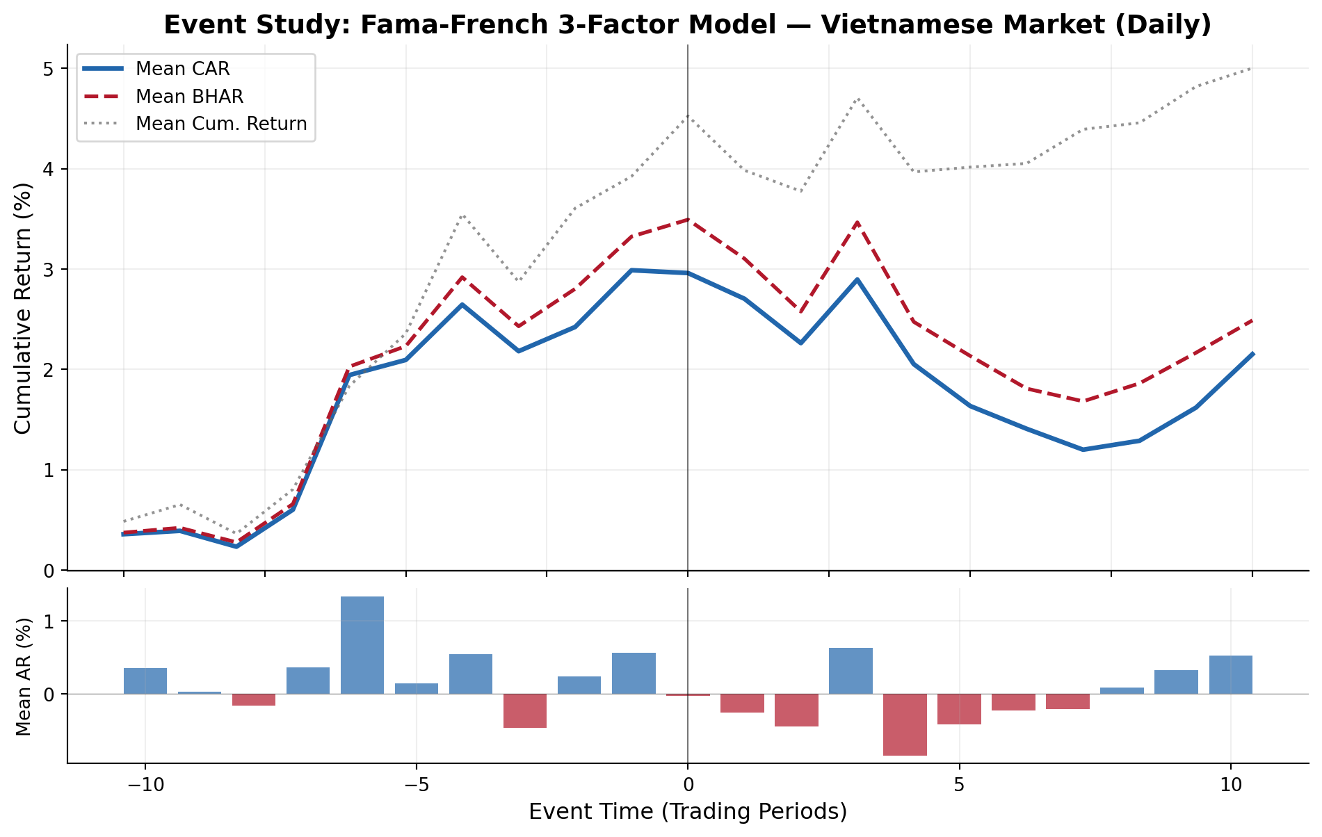
#| fig-cap: "Cumulative abnormal returns around event dates for Vietnamese stocks using the Fama-French 3-factor model. The event window spans [-10, +10] trading days."
fig1 = plot_event_study(
    results_ff3['daily_stats'],
    title="Event Study: Fama-French 3-Factor Model — Vietnamese Market (Daily)"
)
plt.show()
```
```{python}
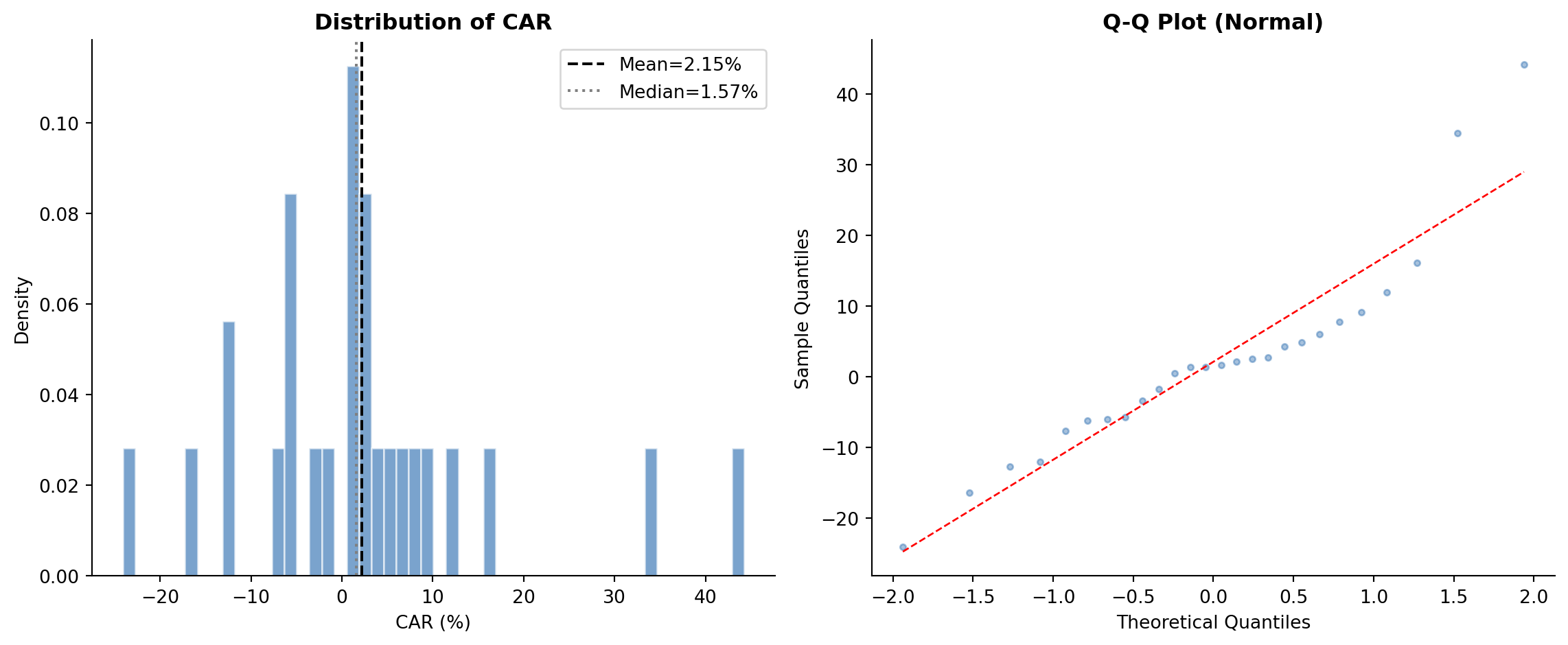
#| label: fig-daily-dist
#| fig-cap: "Cross-sectional distribution of cumulative abnormal returns (CARs) across firm-events. The histogram and Q-Q plot assess normality assumptions underlying parametric tests."
fig2 = plot_car_distribution(results_ff3['event_ar'], 'CAR')
plt.show()
```
### Complete Test Statistics (Daily)
```{python}
#| label: tbl-daily-tests
#| tbl-cap: "Event study test statistics for the full sample and by subgroup — Daily frequency, FF3 model"
ts = results_ff3['test_stats'].copy()

display_cols = ['group', 'N', 'mean_CAR', 'median_CAR', 'mean_BHAR', 'pct_positive',
                't_CS', 'p_CS', 'Z_Patell', 'p_Patell',
                't_BMP', 'p_BMP', 't_KP', 'p_KP',
                'Z_GSign', 'p_GSign', 't_SkAdj', 'p_SkAdj',
                'W_Wilcoxon', 'p_Wilcoxon']
avail = [c for c in display_cols if c in ts.columns]
display_df = ts[avail].copy()

for c in display_df.columns:
    if c in ['N']:
        display_df[c] = display_df[c].astype(int)
    elif c == 'group':
        continue
    elif c.startswith('p_'):
        display_df[c] = display_df[c].map(lambda x: f'{x:.4f}' if pd.notna(x) else '')
    elif c in ['mean_CAR', 'median_CAR', 'mean_BHAR']:
        display_df[c] = display_df[c].map(lambda x: f'{x:.4%}' if pd.notna(x) else '')
    elif c == 'pct_positive':
        display_df[c] = display_df[c].map(lambda x: f'{x:.1%}' if pd.notna(x) else '')
    elif isinstance(display_df[c].iloc[0], (int, float, np.floating)):
        display_df[c] = display_df[c].map(lambda x: f'{x:.3f}' if pd.notna(x) else '')

print(display_df.to_string(index=False))
```
### Robustness: Multiple Risk Models (Daily)
```{python}
#| label: tbl-robustness-daily
#| tbl-cap: "Robustness of event study results across risk models — Daily frequency"
#| code-summary: "Run event study across all available daily models"
models_daily = [
    ("Market-Adjusted",  RiskModel.MARKET_ADJ,    factors_ff3_daily),
    ("Market Model",     RiskModel.MARKET_MODEL,   factors_ff3_daily),
    ("Fama-French 3",    RiskModel.FF3,            factors_ff3_daily),
    ("Fama-French 5",    RiskModel.FF5,            factors_ff5_daily),
]

robustness_daily = []
for name, mdl, facs in models_daily:
    cfg = EventStudyConfig(
        estimation_window=150, event_window_start=-10, event_window_end=10,
        gap=15, min_estimation_obs=120, risk_model=mdl
    )
    res = run_event_study(events_demo, prices_daily, facs, cfg, verbose=False)
    ts = res['test_stats']
    full = ts[ts['group'] == 'All'].iloc[0]
    robustness_daily.append({
        'Model': name,
        'N': int(full['N']),
        'Mean CAR': f"{full['mean_CAR']:.4%}",
        'Median CAR': f"{full['median_CAR']:.4%}",
        'Mean BHAR': f"{full['mean_BHAR']:.4%}",
        '% Positive': f"{full['pct_positive']:.1%}",
        't (CS)': f"{full['t_CS']:.3f}",
        'p (CS)': f"{full['p_CS']:.4f}",
        't (BMP)': f"{full['t_BMP']:.3f}",
        'p (BMP)': f"{full['p_BMP']:.4f}",
        't (KP)': f"{full.get('t_KP', np.nan):.3f}",
        'p (KP)': f"{full.get('p_KP', np.nan):.4f}",
    })

rob_daily_df = pd.DataFrame(robustness_daily)
print("Robustness Across Risk Models (Daily Frequency)")
print("=" * 100)
print(rob_daily_df.to_string(index=False))
```
### Robustness: Multiple Event Windows
A key practice is to examine sensitivity to the event window specification:
```{python}
#| label: tbl-robustness-windows
#| tbl-cap: "Sensitivity of results to event window specification"
#| code-summary: "Test across different event window widths"
windows = [
    ("(-1, +1)",  -1, 1),
    ("(-3, +3)",  -3, 3),
    ("(-5, +5)",  -5, 5),
    ("(-10, +10)", -10, 10),
    ("(-1, +5)",  -1, 5),
    ("(-5, +1)",  -5, 1),
    ("(0, 0)",     0, 0),
]

window_results = []
for label, ws, we in windows:
    cfg = EventStudyConfig(
        estimation_window=150, event_window_start=ws, event_window_end=we,
        gap=15, min_estimation_obs=120, risk_model=RiskModel.FF3
    )
    res = run_event_study(events_demo, prices_daily, factors_ff3_daily, cfg, verbose=False)
    ts = res['test_stats']
    full = ts[ts['group'] == 'All'].iloc[0]
    window_results.append({
        'Window': label,
        'Days': we - ws + 1,
        'N': int(full['N']),
        'Mean CAR': f"{full['mean_CAR']:.4%}",
        'Mean BHAR': f"{full['mean_BHAR']:.4%}",
        '% Positive': f"{full['pct_positive']:.1%}",
        't (CS)': f"{full['t_CS']:.3f}",
        't (BMP)': f"{full['t_BMP']:.3f}",
        'p (BMP)': f"{full['p_BMP']:.4f}",
    })

win_df = pd.DataFrame(window_results)
print("Sensitivity to Event Window Specification (FF3 Model)")
print("=" * 90)
print(win_df.to_string(index=False))
```
### Monthly Event Study: Fama-French 3-Factor Model
For longer-horizon studies, monthly frequency is appropriate. Note that the estimation window is specified in months rather than days:
```{python}
#| label: run-monthly-ff3
#| code-summary: "Run monthly event study with FF3 model"
# Create monthly events aligned to the monthly data
# Map daily event dates to the corresponding month-end
events_monthly = events_demo.copy()
events_monthly['event_date'] = events_monthly['event_date'].dt.to_period('M').dt.to_timestamp('M')

# Use month-end dates from monthly prices
monthly_dates = prices_monthly['date'].sort_values().unique()

# Filter events to dates present in monthly data
events_monthly = events_monthly[events_monthly['event_date'].isin(monthly_dates)]
events_monthly = events_monthly.drop_duplicates(subset=['symbol', 'event_date'])

config_monthly = EventStudyConfig(
    estimation_window=36,     # 36 months
    event_window_start=-3,    # 3 months before
    event_window_end=3,       # 3 months after
    gap=3,                    # 3-month gap
    min_estimation_obs=24,    # At least 24 months
    risk_model=RiskModel.FF3
)

if len(events_monthly) > 0:
    results_monthly = run_event_study(
        events=events_monthly,
        prices=prices_monthly,
        factors=factors_ff3_monthly,
        config=config_monthly,
        group_col='group'
    )

    print("\n--- Monthly Test Statistics ---")
    ts_m = results_monthly['test_stats']
    mcols = ['group', 'N', 'mean_CAR', 'mean_BHAR', 'pct_positive',
             't_CS', 'p_CS', 't_BMP', 'p_BMP']
    mavail = [c for c in mcols if c in ts_m.columns]
    print(ts_m[mavail].to_string(index=False))
else:
    print("No monthly events could be aligned. Skipping monthly study.")
```
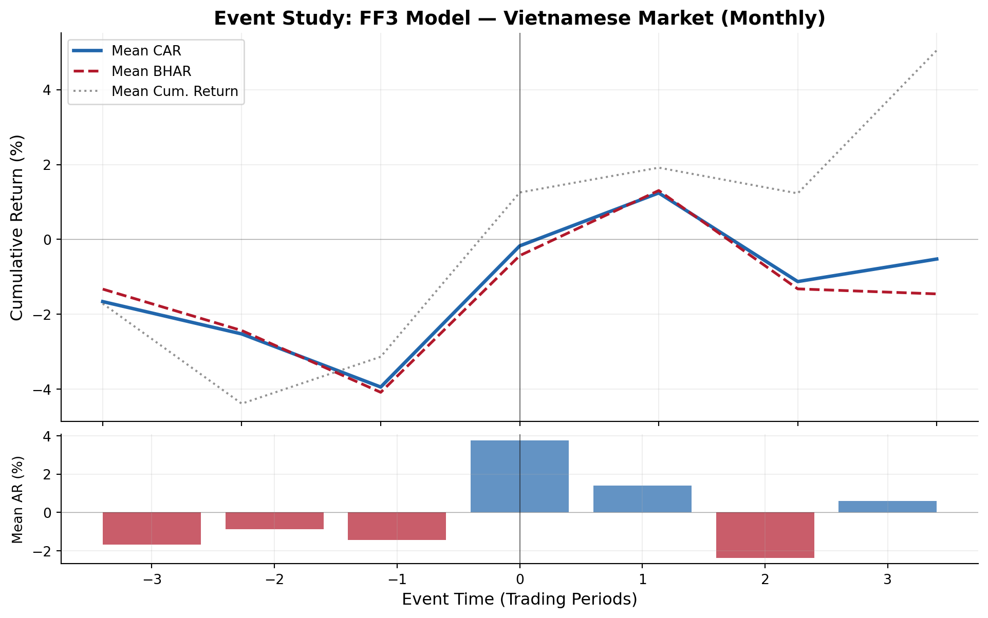
```{python}
#| label: fig-monthly-car
#| fig-cap: "Monthly cumulative abnormal returns around event dates. Wider windows capture slower information incorporation typical of emerging markets."
if len(events_monthly) > 0 and 'daily_stats' in results_monthly:
    fig3 = plot_event_study(
        results_monthly['daily_stats'],
        title="Event Study: FF3 Model — Vietnamese Market (Monthly)"
    )
    plt.show()
```
### Daily Event Study: Fama-French 5-Factor Model
```{python}
#| label: run-daily-ff5
#| code-summary: "Run daily event study with FF5 model"
config_ff5 = EventStudyConfig(
    estimation_window=150,
    event_window_start=-10,
    event_window_end=10,
    gap=15,
    min_estimation_obs=120,
    risk_model=RiskModel.FF5
)

results_ff5 = run_event_study(
    events=events_demo,
    prices=prices_daily,
    factors=factors_ff5_daily,
    config=config_ff5,
    group_col='group'
)
```
### Comparing FF3 vs FF5 Estimation Quality
```{python}
#| label: tbl-model-comparison
#| tbl-cap: "Comparison of estimation quality between FF3 and FF5 models"
params_ff3 = results_ff3['params']
params_ff5 = results_ff5['params']

print("Model Estimation Diagnostics")
print("=" * 60)
print(f"\n{'Metric':<30} {'FF3':>12} {'FF5':>12}")
print("-" * 54)
print(f"{'Firm-events estimated':<30} {len(params_ff3):>12} {len(params_ff5):>12}")
print(f"{'Mean R^2':<30} {params_ff3['r_squared'].mean():>12.4f} {params_ff5['r_squared'].mean():>12.4f}")
print(f"{'Median R^2':<30} {params_ff3['r_squared'].median():>12.4f} {params_ff5['r_squared'].median():>12.4f}")
print(f"{'Mean σ(ε)':<30} {params_ff3['sigma'].mean():>12.6f} {params_ff5['sigma'].mean():>12.6f}")
print(f"{'Mean |α|':<30} {params_ff3['alpha'].abs().mean():>12.6f} {params_ff5['alpha'].abs().mean():>12.6f}")
print(f"{'Mean β(MKT)':<30} {params_ff3['beta_mkt_excess'].mean():>12.4f} {params_ff5['beta_mkt_excess'].mean():>12.4f}")
if 'beta_smb' in params_ff3.columns:
    print(f"{'Mean β(SMB)':<30} {params_ff3['beta_smb'].mean():>12.4f} {params_ff5['beta_smb'].mean():>12.4f}")
if 'beta_hml' in params_ff3.columns:
    print(f"{'Mean β(HML)':<30} {params_ff3['beta_hml'].mean():>12.4f} {params_ff5['beta_hml'].mean():>12.4f}")
if 'beta_rmw' in params_ff5.columns:
    print(f"{'Mean β(RMW)':<30} {'—':>12} {params_ff5['beta_rmw'].mean():>12.4f}")
if 'beta_cma' in params_ff5.columns:
    print(f"{'Mean β(CMA)':<30} {'—':>12} {params_ff5['beta_cma'].mean():>12.4f}")
```
### Event-Level Detail
```{python}
#| label: tbl-event-detail
#| tbl-cap: "Event-level detail: CARs and BHARs for each firm-event (FF3 model)"
detail = results_ff3['event_ar'].copy()
detail_cols = ['symbol', 'evtdate', 'CAR', 'BHAR', 'SCAR', 'sigma',
               'nobs', 'alpha', 'beta_mkt_excess']
detail_avail = [c for c in detail_cols if c in detail.columns]
detail_show = detail[detail_avail].copy()
detail_show['CAR'] = detail_show['CAR'].map(lambda x: f'{x:.4%}')
detail_show['BHAR'] = detail_show['BHAR'].map(lambda x: f'{x:.4%}')
detail_show['SCAR'] = detail_show['SCAR'].map(lambda x: f'{x:.3f}')

print("Event-Level Results (first 20 firm-events)")
print("=" * 100)
print(detail_show.head(20).to_string(index=False))
```
### Daily Abnormal Return Dynamics
```{python}
#| label: tbl-daily-dynamics
#| tbl-cap: "Daily dynamics of mean abnormal returns and test statistics within the event window"
ds = results_ff3['daily_stats'].copy()
ds_cols = ['evttime', 'N', 'mean_AR', 'mean_CAR', 'mean_BHAR', 't_AR_CS', 't_AR_BMP']
ds_avail = [c for c in ds_cols if c in ds.columns]
ds_show = ds[ds_avail].copy()

for c in ['mean_AR', 'mean_CAR', 'mean_BHAR']:
    if c in ds_show.columns:
        ds_show[c] = ds_show[c].map(lambda x: f'{x:.4%}')
for c in ['t_AR_CS', 't_AR_BMP']:
    if c in ds_show.columns:
        ds_show[c] = ds_show[c].map(lambda x: f'{x:.3f}' if pd.notna(x) else '')

print("Daily Event-Window Dynamics (FF3 Model)")
print("=" * 80)
print(ds_show.to_string(index=False))
```
### Summary of Key Findings
```{python}
#| label: summary
#| code-summary: "Summarize key findings"
print("=" * 70)
print("EVENT STUDY RESULTS SUMMARY")
print("=" * 70)

ff3_all = results_ff3['test_stats'][results_ff3['test_stats']['group'] == 'All'].iloc[0]

print(f"\nSample: {int(ff3_all['N'])} firm-event observations")
print(f"Frequency: Daily")
print(f"Primary Model: Fama-French 3-Factor")
print(f"Estimation Window: {config_ff3.estimation_window} trading days")
print(f"Event Window: ({config_ff3.event_window_start}, {config_ff3.event_window_end})")
print(f"Gap: {config_ff3.gap} trading days")
print(f"\n--- Abnormal Return Measures ---")
print(f"Mean CAR({config_ff3.event_window_start},{config_ff3.event_window_end}): "
      f"{ff3_all['mean_CAR']:.4%}")
print(f"Median CAR: {ff3_all['median_CAR']:.4%}")
print(f"Mean BHAR: {ff3_all['mean_BHAR']:.4%}")
print(f"Fraction positive CARs: {ff3_all['pct_positive']:.1%}")
print(f"\n--- Statistical Significance ---")
print(f"Cross-Sectional t: {ff3_all['t_CS']:.3f} (p = {ff3_all['p_CS']:.4f})")
print(f"Patell Z: {ff3_all['Z_Patell']:.3f} (p = {ff3_all['p_Patell']:.4f})")
print(f"BMP t: {ff3_all['t_BMP']:.3f} (p = {ff3_all['p_BMP']:.4f})")
print(f"Kolari-Pynnönen t: {ff3_all['t_KP']:.3f} (p = {ff3_all['p_KP']:.4f})")
print(f"Generalized Sign Z: {ff3_all['Z_GSign']:.3f} (p = {ff3_all['p_GSign']:.4f})")

sig_005 = sum(1 for k in ['p_CS','p_Patell','p_BMP','p_KP','p_GSign','p_SkAdj','p_Wilcoxon']
              if k in ff3_all and pd.notna(ff3_all[k]) and ff3_all[k] < 0.05)
total_tests = sum(1 for k in ['p_CS','p_Patell','p_BMP','p_KP','p_GSign','p_SkAdj','p_Wilcoxon']
                  if k in ff3_all and pd.notna(ff3_all[k]))
print(f"\n{sig_005}/{total_tests} tests significant at 5% level")

# Robustness note
print(f"\nRobustness: Results checked across {len(models_daily)} risk models "
      f"and {len(windows)} event windows")
```
## Practical Recommendations
Based on the literature and our implementation experience:
1. **Estimation window**: Use 150 trading days (\~7 months) for daily studies. This balances parameter precision against structural breaks. For monthly studies, 60 months is standard [@kothari2007econometrics].
2. **Gap**: 15 trading days is standard. Increase to 30 if information leakage is a concern.
3. **Event window**: Start with (-1, +1) for short-window tests, then expand to (-5, +5) and (-10, +10) for robustness. Report all windows.
4. **Model choice**: Always report market model as the baseline. Add FF3 or FF5 for robustness. For Vietnam, local factors are preferable to global factors.
5. **Test statistics**: Report at minimum: cross-sectional t (for ease of interpretation), BMP (robust to event-induced variance), and one non-parametric test (sign or Wilcoxon). Report Kolari-Pynnönen if events cluster in calendar time.
6. **Thin trading**: For Vietnamese small-caps, consider @dimson1979risk with 1 lead/lag or increase `min_estimation_obs` to filter out illiquid stocks.
7. **Multiple testing**: If testing multiple event windows or subgroups, apply Bonferroni or Holm corrections to control family-wise error rate.