import pandas as pd
import numpy as np
import sqlite3
import statsmodels.formula.api as smf
from scipy.stats.mstats import winsorize
import matplotlib.pyplot as plt

from plotnine import *
from mizani.formatters import percent_format, comma_format17 Fama-French Factors
This chapter provides a replication of the Fama-French factor portfolios for the Vietnamese stock market. The Fama-French factor models represent a cornerstone of empirical asset pricing, originating from the seminal work of Fama and French (1992) and later extended in Fama and French (2015). These models have transformed how academics and practitioners understand the cross-section of expected stock returns, moving beyond the single-factor Capital Asset Pricing Model to incorporate multiple sources of systematic risk.
We construct both the three-factor and five-factor models at monthly and daily frequencies. The monthly factors serve as the foundation for most asset pricing tests and portfolio analyses, while the daily factors enable higher-frequency applications including short-horizon event studies, market microstructure research, and daily beta estimation. By constructing factors at both frequencies, we create a complete toolkit for empirical finance research in the Vietnamese market.
The chapter proceeds as follows. We first discuss the theoretical motivation for each factor and the economic intuition behind the Fama-French methodology. We then prepare the necessary data, merging stock returns with accounting characteristics. Next, we implement the portfolio sorting procedures that form the basis of factor construction, carefully following the original Fama-French protocols while adapting them for Vietnamese market characteristics. We construct the three-factor model (market, size, and value) before extending to the five-factor model (adding profitability and investment). Finally, we construct daily factors and validate our replicated factors through various diagnostic checks.
17.1 Theoretical Background
17.1.1 The Evolution from CAPM to Multi-Factor Models
The Capital Asset Pricing Model of Sharpe (1964) posits that a single factor—the market portfolio—should explain all cross-sectional variation in expected returns. However, decades of empirical research have documented persistent patterns that CAPM cannot explain. Fama and French (1992) demonstrated that two firm characteristics—size and book-to-market ratio—capture substantial variation in average returns that the market beta leaves unexplained.
Small firms tend to earn higher returns than large firms, a pattern known as the size effect. Similarly, firms with high book-to-market ratios (value stocks) tend to outperform firms with low book-to-market ratios (growth stocks), known as the value premium. The three-factor model formalizes these observations by constructing tradeable factor portfolios:
\[ r_{i,t} - r_{f,t} = \alpha_i + \beta_i^{MKT}(r_{m,t} - r_{f,t}) + \beta_i^{SMB} \cdot SMB_t + \beta_i^{HML} \cdot HML_t + \varepsilon_{i,t} \tag{17.1}\]
where:
- \(r_{i,t} - r_{f,t}\) is the excess return on asset \(i\)
- \(r_{m,t} - r_{f,t}\) is the market excess return
- \(SMB_t\) (Small Minus Big) is the size factor
- \(HML_t\) (High Minus Low) is the value factor
17.1.2 The Five-Factor Extension
Fama and French (2015) extended the model to include two additional factors motivated by the dividend discount model. Firms with higher profitability should have higher expected returns (all else equal), and firms with aggressive investment policies should have lower expected returns:
\[ r_{i,t} - r_{f,t} = \alpha_i + \beta_i^{MKT}MKT_t + \beta_i^{SMB}SMB_t + \beta_i^{HML}HML_t + \beta_i^{RMW}RMW_t + \beta_i^{CMA}CMA_t + \varepsilon_{i,t} \tag{17.2}\]
where:
- \(RMW_t\) (Robust Minus Weak) is the profitability factor
- \(CMA_t\) (Conservative Minus Aggressive) is the investment factor
17.1.3 Factor Construction Methodology
The Fama-French methodology constructs factors through double-sorted portfolios:
Size sorts: Stocks are divided into Small and Big groups based on median market capitalization.
Characteristic sorts: Within each size group, stocks are sorted into terciles based on book-to-market (for HML), operating profitability (for RMW), or investment (for CMA).
Factor returns: Factors are computed as the difference between average returns of portfolios with high versus low characteristic values, averaging across size groups to neutralize size effects.
Timing: Portfolios are formed at the end of June each year using accounting data from the prior fiscal year, ensuring all information was publicly available at formation.
17.2 Setting Up the Environment
We load the required Python packages for data manipulation, statistical analysis, and visualization.
We connect to our SQLite database containing the processed Vietnamese financial data.
tidy_finance = sqlite3.connect(database="data/tidy_finance_python.sqlite")17.3 Data Preparation
17.3.1 Loading Stock Returns
We load the monthly stock returns data, which includes excess returns, market capitalization, and the risk-free rate. These variables are essential for computing value-weighted portfolio returns and factor premiums.
prices_monthly = pd.read_sql_query(
    sql="""
        SELECT symbol, date, ret_excess, mktcap, mktcap_lag, risk_free
        FROM prices_monthly
    """,
    con=tidy_finance,
    parse_dates={"date"}
).dropna()

print(f"Monthly returns: {len(prices_monthly):,} observations")
print(f"Unique stocks: {prices_monthly['symbol'].nunique():,}")
print(f"Date range: {prices_monthly['date'].min():%Y-%m} to {prices_monthly['date'].max():%Y-%m}")
Monthly returns: 165,499 observations
Unique stocks: 1,457
Date range: 2010-02 to 2023-1217.3.2 Loading Company Fundamentals
We load the company fundamentals data containing book equity, operating profitability, and investment—the characteristics needed for constructing the Fama-French factors.
comp_vn = pd.read_sql_query(
    sql="""
        SELECT symbol, datadate, be, op, inv
        FROM comp_vn
    """,
    con=tidy_finance,
    parse_dates={"datadate"}
).dropna()

print(f"Fundamentals: {len(comp_vn):,} firm-year observations")
print(f"Unique firms: {comp_vn['symbol'].nunique():,}")
Fundamentals: 18,108 firm-year observations
Unique firms: 1,49617.3.3 Constructing Sorting Variables
Following Fama-French conventions, we construct the sorting variables with careful attention to timing. The key principles are:
Size (June Market Cap): We use market capitalization at the end of June of year \(t\) to sort stocks into size groups. This ensures we capture the firm’s size at the moment of portfolio formation.
Book-to-Market Ratio: We use book equity from fiscal year \(t-1\) divided by market equity at the end of December \(t-1\). This creates a six-month gap between the accounting data and portfolio formation, ensuring the information was publicly available.
Portfolio Formation Date: Portfolios are formed on July 1st and held for twelve months until the following June.
def construct_sorting_variables(prices_monthly, comp_vn):
    """
    Construct sorting variables following Fama-French methodology.

    Parameters
    ----------
    prices_monthly : pd.DataFrame
        Monthly stock returns with market cap
    comp_vn : pd.DataFrame
        Company fundamentals with book equity, profitability, investment

    Returns
    -------
    pd.DataFrame
        Sorting variables aligned with July 1st formation dates
    """

    # 1. Size: June market capitalization
    # Portfolio formation is July 1st, so we use June market cap
    size = (prices_monthly
        .query("date.dt.month == 6")
        .assign(
            sorting_date=lambda x: x["date"] + pd.offsets.MonthBegin(1)
        )
        [["symbol", "sorting_date", "mktcap"]]
        .rename(columns={"mktcap": "size"})
    )

    print(f"Size observations: {len(size):,}")

    # 2. Market Equity: December market cap for B/M calculation
    # December t-1 market cap is used with fiscal year t-1 book equity
    # This is then used for July t portfolio formation
    market_equity = (prices_monthly
        .query("date.dt.month == 12")
        .assign(
            # December year t-1 maps to July year t formation
            sorting_date=lambda x: x["date"] + pd.offsets.MonthBegin(7)
        )
        [["symbol", "sorting_date", "mktcap"]]
        .rename(columns={"mktcap": "me"})
    )

    print(f"Market equity observations: {len(market_equity):,}")

    # 3. Book-to-Market and other characteristics
    # Fiscal year t-1 data is used for July t portfolio formation
    book_to_market = (comp_vn
        .assign(
            # Fiscal year-end + 6 months = July formation
            sorting_date=lambda x: pd.to_datetime(
                (x["datadate"].dt.year + 1).astype(str) + "-07-01"
            )
        )
        .merge(market_equity, on=["symbol", "sorting_date"], how="inner")
        .assign(
            # Scale book equity to match market equity units
            # BE is in VND, ME is in millions VND
            bm=lambda x: x["be"] / (x["me"] * 1e9)
        )
        [["symbol", "sorting_date", "me", "bm", "op", "inv"]]
    )

    print(f"Book-to-market observations: {len(book_to_market):,}")

    # 4. Merge size with characteristics
    sorting_variables = (size
        .merge(book_to_market, on=["symbol", "sorting_date"], how="inner")
        .dropna()
        .drop_duplicates(subset=["symbol", "sorting_date"])
    )

    return sorting_variables

sorting_variables = construct_sorting_variables(prices_monthly, comp_vn)

print(f"\nFinal sorting variables: {len(sorting_variables):,} stock-years")
print(f"Sorting date range: {sorting_variables['sorting_date'].min():%Y-%m} to {sorting_variables['sorting_date'].max():%Y-%m}")
Size observations: 13,756
Market equity observations: 14,286
Book-to-market observations: 13,389
Final sorting variables: 12,046 stock-years
Sorting date range: 2011-07 to 2023-0717.3.4 Validating Sorting Variables
Before proceeding, we validate that our sorting variables have reasonable distributions. The book-to-market ratio should center around 1.0 for a typical market, though emerging markets may differ.
print("Sorting Variable Summary Statistics:")
print(sorting_variables[["size", "bm", "op", "inv"]].describe().round(4))

# Check for extreme values that might indicate data issues
print(f"\nB/M Median: {sorting_variables['bm'].median():.4f}")
print(f"B/M 1st percentile: {sorting_variables['bm'].quantile(0.01):.4f}")
print(f"B/M 99th percentile: {sorting_variables['bm'].quantile(0.99):.4f}")
Sorting Variable Summary Statistics:
size bm op inv
count 12046.0000 12046.0000 12046.0000 12046.0000
mean 2225.5648 1.7033 0.1852 0.1322
std 14680.4225 3.8683 0.2782 2.5410
min 0.4864 0.0014 -0.7529 -0.9569
25% 62.7556 0.7595 0.0309 -0.0495
50% 182.6410 1.1849 0.1367 0.0342
75% 641.8896 1.8853 0.2952 0.1582
max 426020.9817 272.1893 1.4256 261.3355
B/M Median: 1.1849
B/M 1st percentile: 0.1710
B/M 99th percentile: 8.026217.3.5 Handling Outliers
Extreme values in sorting characteristics can distort portfolio assignments and factor returns. We apply winsorization to limit the influence of outliers while preserving the general ranking of stocks.
# Check BEFORE winsorization
print("BEFORE Winsorization:")
print(sorting_variables[["size", "bm", "op", "inv"]].describe().round(4))

# Apply winsorization
def winsorize_characteristics(df, columns, limits=(0.01, 0.99)):
    """
    Apply winsorization using pandas clip.
    """
    df = df.copy()
    for col in columns:
        if col in df.columns:
            lower = df[col].quantile(limits[0])
            upper = df[col].quantile(limits[1])
            df[col] = df[col].clip(lower=lower, upper=upper)
            print(f"  {col}: clipped to [{lower:.4f}, {upper:.4f}]")
    return df

sorting_variables = winsorize_characteristics(
    sorting_variables,
    columns=["bm", "op", "inv"],  # Don't winsorize size
    limits=(0.01, 0.99)
)

# Check AFTER winsorization
print("\nAFTER Winsorization:")
print(sorting_variables[["size", "bm", "op", "inv"]].describe().round(4))
BEFORE Winsorization:
size bm op inv
count 12046.0000 12046.0000 12046.0000 12046.0000
mean 2225.5648 1.7033 0.1852 0.1322
std 14680.4225 3.8683 0.2782 2.5410
min 0.4864 0.0014 -0.7529 -0.9569
25% 62.7556 0.7595 0.0309 -0.0495
50% 182.6410 1.1849 0.1367 0.0342
75% 641.8896 1.8853 0.2952 0.1582
max 426020.9817 272.1893 1.4256 261.3355
bm: clipped to [0.1710, 8.0262]
op: clipped to [-0.7319, 1.2192]
inv: clipped to [-0.3990, 1.5195]
AFTER Winsorization:
size bm op inv
count 12046.0000 12046.0000 12046.0000 12046.0000
mean 2225.5648 1.5544 0.1837 0.0894
std 14680.4225 1.2843 0.2705 0.2721
min 0.4864 0.1710 -0.7319 -0.3990
25% 62.7556 0.7595 0.0309 -0.0495
50% 182.6410 1.1849 0.1367 0.0342
75% 641.8896 1.8853 0.2952 0.1582
max 426020.9817 8.0262 1.2192 1.519517.4 Portfolio Assignment Functions
17.4.1 The Portfolio Assignment Function
We create a flexible function for assigning stocks to portfolios based on quantile breakpoints. This function handles both independent sorts (where breakpoints are computed across all stocks) and dependent sorts (where breakpoints are computed within subgroups).
def assign_portfolio(data, sorting_variable, percentiles):
    """Assign portfolios to a bin according to a sorting variable."""

    # Get the values
    values = data[sorting_variable].dropna()

    if len(values) == 0:
        return pd.Series([np.nan] * len(data), index=data.index)

    # Calculate breakpoints
    breakpoints = values.quantile(percentiles, interpolation="linear")

    # Handle duplicate breakpoints by using unique values
    unique_breakpoints = np.unique(breakpoints)

    # If all values are the same, assign all to portfolio 1
    if len(unique_breakpoints) <= 1:
        return pd.Series([1] * len(data), index=data.index)

    # Set boundaries to -inf and +inf
    unique_breakpoints.iloc[0] = -np.inf
    unique_breakpoints.iloc[unique_breakpoints.size-1] = np.inf

    # Assign to bins
    assigned = pd.cut(
        data[sorting_variable],
        bins=unique_breakpoints,
        labels=pd.Series(range(1, breakpoints.size)),
        include_lowest=True,
        right=False
    )

    return assigned
# Check the distribution of characteristics BEFORE portfolio assignment
print("Operating Profitability Distribution:")
print(sorting_variables["op"].describe())
print(f"\nUnique OP values: {sorting_variables['op'].nunique()}")
print("\nInvestment Distribution:")
print(sorting_variables["inv"].describe())
print(f"\nUnique INV values: {sorting_variables['inv'].nunique()}")
# Check breakpoints for a specific date
test_date = sorting_variables["sorting_date"].iloc[0]
test_data = sorting_variables.query("sorting_date == @test_date")
print(f"\nBreakpoints for {test_date}:")
print(f"OP 30th percentile: {test_data['op'].quantile(0.3):.4f}")
print(f"OP 70th percentile: {test_data['op'].quantile(0.7):.4f}")
print(f"INV 30th percentile: {test_data['inv'].quantile(0.3):.4f}")
print(f"INV 70th percentile: {test_data['inv'].quantile(0.7):.4f}")Operating Profitability Distribution:
count 12046.000000
mean 0.183738
std 0.270509
min -0.731888
25% 0.030913
50% 0.136675
75% 0.295185
max 1.219223
Name: op, dtype: float64
Unique OP values: 11804
Investment Distribution:
count 12046.000000
mean 0.089388
std 0.272147
min -0.399042
25% -0.049497
50% 0.034157
75% 0.158155
max 1.519474
Name: inv, dtype: float64
Unique INV values: 11805
Breakpoints for 2019-07-01 00:00:00:
OP 30th percentile: 0.0541
OP 70th percentile: 0.2566
INV 30th percentile: -0.0343
INV 70th percentile: 0.111617.4.2 Assigning Portfolios for Three-Factor Model
For the three-factor model, we perform independent double sorts on size and book-to-market. Size is split at the median (2 groups), and book-to-market is split at the 30th and 70th percentiles (3 groups), creating 6 portfolios.
def assign_ff3_portfolios(sorting_variables):
    """
    Assign portfolios for Fama-French three-factor model.
    Independent 2x3 sort on size and book-to-market.
    """
    df = sorting_variables.copy()

    # Independent size sort (median split)
    df["portfolio_size"] = df.groupby("sorting_date")["size"].transform(
        lambda x: pd.qcut(x, q=[0, 0.5, 1], labels=[1, 2], duplicates='drop')
    )

    # Independent B/M sort (30/70 split)
    df["portfolio_bm"] = df.groupby("sorting_date")["bm"].transform(
        lambda x: pd.qcut(x, q=[0, 0.3, 0.7, 1], labels=[1, 2, 3], duplicates='drop')
    )

    return df

# Assign portfolios
portfolios_ff3 = assign_ff3_portfolios(sorting_variables)

# Validate
print("FF3 Book-to-Market by Portfolio (should be INCREASING):")
print(portfolios_ff3.groupby("portfolio_bm", observed=True)["bm"].median().round(4))


print("Three-Factor Portfolio Assignments:")
print(portfolios_ff3[["symbol", "sorting_date", "portfolio_size", "portfolio_bm"]].head(10))
FF3 Book-to-Market by Portfolio (should be INCREASING):
portfolio_bm
1 0.5836
2 1.1891
3 2.4552
Name: bm, dtype: float64
Three-Factor Portfolio Assignments:
symbol sorting_date portfolio_size portfolio_bm
0 A32 2019-07-01 1 2
1 A32 2020-07-01 1 2
2 A32 2021-07-01 1 2
3 A32 2022-07-01 1 3
4 A32 2023-07-01 1 2
5 AAA 2011-07-01 2 2
6 AAA 2012-07-01 2 3
7 AAA 2013-07-01 2 3
8 AAA 2014-07-01 2 2
9 AAA 2015-07-01 2 317.4.3 Validating Portfolio Assignments
We verify that the portfolio assignments create the expected 2×3 grid with reasonable stock counts in each cell.
# Check portfolio distribution for most recent year
latest_date = portfolios_ff3["sorting_date"].max()

portfolio_counts = (portfolios_ff3
    .query("sorting_date == @latest_date")
    .groupby(["portfolio_size", "portfolio_bm"], observed=True)
    .size()
    .unstack(fill_value=0)
)

print(f"Portfolio Counts for {latest_date:%Y-%m}:")
print(portfolio_counts)

# Verify characteristic monotonicity
print("\nBook-to-Market by Portfolio (should be increasing):")
print(portfolios_ff3.groupby("portfolio_bm", observed=True)["bm"].median().round(4))
Portfolio Counts for 2023-07:
portfolio_bm 1 2 3
portfolio_size
1 113 271 263
2 275 246 125
Book-to-Market by Portfolio (should be increasing):
portfolio_bm
1 0.5836
2 1.1891
3 2.4552
Name: bm, dtype: float64We verify that for a single stock, the portfolio assignment remains constant between July of one year and June of the next.
# Trace a single symbol (e.g., 'A32') across a formation window
persistence_check = (portfolios_ff3
    .query("symbol == 'A32' & sorting_date >= '2022-01-01' & sorting_date <= '2023-12-31'")
    .sort_values("sorting_date")
    [['symbol', 'sorting_date', 'portfolio_size', 'portfolio_bm']]
)
print("\nTemporal Persistence Check (Symbol A32):")
print(persistence_check.head(15))
Temporal Persistence Check (Symbol A32):
  symbol sorting_date portfolio_size portfolio_bm
3    A32   2022-07-01              1            3
4    A32   2023-07-01              1            2
17.5 Fama-French Three-Factor Model (Monthly)
17.5.1 Merging Portfolios with Returns
We merge the portfolio assignments with monthly returns. The key insight is that portfolios formed in July of year \(t\) are held through June of year \(t+1\). We implement this by computing a sorting_date for each monthly return observation.
def merge_portfolios_with_returns(prices_monthly, portfolio_assignments):
    """
    Merge portfolio assignments with monthly returns.

    Portfolios formed in July t are held through June t+1.

    Parameters
    ----------
    prices_monthly : pd.DataFrame
        Monthly stock returns
    portfolio_assignments : pd.DataFrame
        Portfolio assignments with sorting_date

    Returns
    -------
    pd.DataFrame
        Returns merged with portfolio assignments
    """
    portfolios = (prices_monthly
        .assign(
            # Map each return month to its portfolio formation date
            sorting_date=lambda x: pd.to_datetime(
                np.where(
                    x["date"].dt.month <= 6,
                    (x["date"].dt.year - 1).astype(str) + "-07-01",
                    x["date"].dt.year.astype(str) + "-07-01"
                )
            )
        )
        .merge(
            portfolio_assignments,
            on=["symbol", "sorting_date"],
            how="inner"
        )
    )

    return portfolios

portfolios_monthly_ff3 = merge_portfolios_with_returns(
    prices_monthly,
    portfolios_ff3[["symbol", "sorting_date", "portfolio_size", "portfolio_bm"]]
)


print(f"Merged observations: {len(portfolios_monthly_ff3):,}")
Merged observations: 136,44417.5.2 Computing Value-Weighted Portfolio Returns
We compute value-weighted returns for each of the six portfolios. Value-weighting uses lagged market capitalization to avoid look-ahead bias.
def compute_portfolio_returns(data, grouping_vars):
    """
    Compute value-weighted portfolio returns.

    Parameters
    ----------
    data : pd.DataFrame
        Returns data with portfolio assignments and mktcap_lag
    grouping_vars : list
        Variables defining portfolio groups

    Returns
    -------
    pd.DataFrame
        Value-weighted returns for each portfolio-date
    """
    portfolio_returns = (data
        .groupby(grouping_vars + ["date"], observed=True)
        .apply(lambda x: pd.Series({
            "ret": np.average(x["ret_excess"], weights=x["mktcap_lag"]),
            "n_stocks": len(x)
        }))
        .reset_index()
    )

    return portfolio_returns


# Compute portfolio returns
portfolio_returns_ff3 = compute_portfolio_returns(
    portfolios_monthly_ff3,
    ["portfolio_size", "portfolio_bm"]
)

print("Portfolio Returns Summary:")
print(portfolio_returns_ff3.groupby(["portfolio_size", "portfolio_bm"], observed=True)["ret"].describe().round(4))
Portfolio Returns Summary:
count mean std min 25% 50% \
portfolio_size portfolio_bm
1 1 150.0 -0.0052 0.0379 -0.1268 -0.0262 -0.0058
2 150.0 -0.0025 0.0414 -0.1080 -0.0236 -0.0053
3 150.0 0.0039 0.0601 -0.1612 -0.0269 -0.0004
2 1 150.0 -0.0124 0.0594 -0.2222 -0.0449 -0.0107
2 150.0 -0.0021 0.0671 -0.1701 -0.0403 -0.0046
3 150.0 0.0024 0.0879 -0.2359 -0.0527 -0.0012
75% max
portfolio_size portfolio_bm
1 1 0.0161 0.0849
2 0.0180 0.1195
3 0.0314 0.2015
2 1 0.0210 0.1741
2 0.0317 0.1770
3 0.0437 0.2124 17.5.3 Constructing SMB and HML Factors
We now construct the SMB and HML factors from the portfolio returns.
SMB (Small Minus Big): Average return of three small portfolios minus average return of three big portfolios.
HML (High Minus Low): Average return of two high B/M portfolios minus average return of two low B/M portfolios.
def construct_ff3_factors(portfolio_returns):
    """
    Construct Fama-French three factors from portfolio returns.

    Parameters
    ----------
    portfolio_returns : pd.DataFrame
        Value-weighted returns for 2x3 portfolios

    Returns
    -------
    pd.DataFrame
        Monthly SMB and HML factors
    """
    factors = (portfolio_returns
        .groupby("date")
        .apply(lambda x: pd.Series({
            # SMB: Small minus Big (average across B/M groups)
            "smb": (
                x.loc[x["portfolio_size"] == 1, "ret"].mean() -
                x.loc[x["portfolio_size"] == 2, "ret"].mean()
            ),
            # HML: High minus Low B/M (average across size groups)
            "hml": (
                x.loc[x["portfolio_bm"] == 3, "ret"].mean() -
                x.loc[x["portfolio_bm"] == 1, "ret"].mean()
            )
        }))
        .reset_index()
    )

    return factors

factors_smb_hml = construct_ff3_factors(portfolio_returns_ff3)

print("SMB and HML Factors:")
print(factors_smb_hml.head(10))
SMB and HML Factors:
date smb hml
0 2011-07-31 -0.007768 0.002754
1 2011-08-31 -0.067309 0.011474
2 2011-09-30 0.014884 0.022854
3 2011-10-31 -0.003743 0.001631
4 2011-11-30 0.063234 0.009103
5 2011-12-31 0.014571 0.015280
6 2012-01-31 -0.026080 0.009672
7 2012-02-29 -0.035721 0.005474
8 2012-03-31 -0.002344 0.032477
9 2012-04-30 -0.033391 0.07419117.5.4 Computing the Market Factor
The market factor is the value-weighted return of all stocks minus the risk-free rate. We compute this independently from the sorted portfolios.
def compute_market_factor(prices_monthly):
    """
    Compute value-weighted market excess return.

    Parameters
    ----------
    prices_monthly : pd.DataFrame
        Monthly stock returns with mktcap_lag

    Returns
    -------
    pd.DataFrame
        Monthly market excess return
    """
    market_factor = (prices_monthly
        .groupby("date")
        .apply(lambda x: pd.Series({
            "mkt_excess": np.average(x["ret_excess"], weights=x["mktcap_lag"]),
            "n_stocks": len(x)
        }), include_groups=False)
        .reset_index()
    )

    return market_factor

market_factor = compute_market_factor(prices_monthly)

print("Market Factor Summary:")
print(market_factor["mkt_excess"].describe().round(4))
Market Factor Summary:
count 167.0000
mean -0.0123
std 0.0595
min -0.2149
25% -0.0394
50% -0.0106
75% 0.0200
max 0.1677
Name: mkt_excess, dtype: float6417.5.5 Combining Three Factors
We combine SMB, HML, and the market factor into the complete three-factor dataset.
factors_ff3_monthly = (factors_smb_hml
    .merge(market_factor[["date", "mkt_excess"]], on="date", how="inner")
)

# Add risk-free rate for completeness
rf_monthly = (prices_monthly
    .groupby("date")["risk_free"]
    .first()
    .reset_index()
)

factors_ff3_monthly = factors_ff3_monthly.merge(rf_monthly, on="date", how="left")

print("Fama-French Three Factors (Monthly):")
print(factors_ff3_monthly.head(10))

print("\nFactor Summary Statistics:")
print(factors_ff3_monthly[["mkt_excess", "smb", "hml"]].describe().round(4))
Fama-French Three Factors (Monthly):
date smb hml mkt_excess risk_free
0 2011-07-31 -0.007768 0.002754 -0.078748 0.003333
1 2011-08-31 -0.067309 0.011474 0.029906 0.003333
2 2011-09-30 0.014884 0.022854 -0.002173 0.003333
3 2011-10-31 -0.003743 0.001631 -0.014005 0.003333
4 2011-11-30 0.063234 0.009103 -0.179410 0.003333
5 2011-12-31 0.014571 0.015280 -0.094802 0.003333
6 2012-01-31 -0.026080 0.009672 0.081273 0.003333
7 2012-02-29 -0.035721 0.005474 0.069655 0.003333
8 2012-03-31 -0.002344 0.032477 0.029005 0.003333
9 2012-04-30 -0.033391 0.074191 0.048791 0.003333
Factor Summary Statistics:
mkt_excess smb hml
count 150.0000 150.0000 150.0000
mean -0.0101 0.0027 0.0120
std 0.0586 0.0420 0.0535
min -0.2149 -0.1599 -0.1284
25% -0.0380 -0.0175 -0.0160
50% -0.0095 0.0070 0.0043
75% 0.0214 0.0261 0.0340
max 0.1677 0.1175 0.161817.5.6 Saving Three-Factor Data
factors_ff3_monthly.to_sql(
    name="factors_ff3_monthly",
    con=tidy_finance,
    if_exists="replace",
    index=False
)

print("Three-factor monthly data saved to database.")
Three-factor monthly data saved to database.17.6 Fama-French Five-Factor Model (Monthly)
17.6.1 Portfolio Assignments with Dependent Sorts
For the five-factor model, we use dependent sorts: size is sorted independently, but profitability and investment are sorted within size groups. This controls for the correlation between size and these characteristics.
def assign_ff5_portfolios(sorting_variables):
    """
    Assign portfolios for Fama-French five-factor model.
    """
    df = sorting_variables.copy()

    # Independent size sort
    df["portfolio_size"] = df.groupby("sorting_date")["size"].transform(
        lambda x: pd.qcut(x, q=[0, 0.5, 1], labels=[1, 2], duplicates='drop')
    )

    # Dependent sorts within size groups
    df["portfolio_bm"] = df.groupby(["sorting_date", "portfolio_size"])["bm"].transform(
        lambda x: pd.qcut(x, q=[0, 0.3, 0.7, 1], labels=[1, 2, 3], duplicates='drop')
    )

    df["portfolio_op"] = df.groupby(["sorting_date", "portfolio_size"])["op"].transform(
        lambda x: pd.qcut(x, q=[0, 0.3, 0.7, 1], labels=[1, 2, 3], duplicates='drop')
    )

    df["portfolio_inv"] = df.groupby(["sorting_date", "portfolio_size"])["inv"].transform(
        lambda x: pd.qcut(x, q=[0, 0.3, 0.7, 1], labels=[1, 2, 3], duplicates='drop')
    )

    return df

# Run
portfolios_ff5 = assign_ff5_portfolios(sorting_variables)
17.6.2 Validating Five-Factor Portfolios
# Check characteristic monotonicity for each dimension
print("Profitability by Portfolio (should be increasing):")
print(portfolios_ff5.groupby("portfolio_op", observed=True)["op"].median().round(4))

print("\nInvestment by Portfolio (should be increasing):")
print(portfolios_ff5.groupby("portfolio_inv", observed=True)["inv"].median().round(4))

# Check portfolio counts
print("\nStocks per Size/Profitability Bin:")
print(portfolios_ff5.groupby(["portfolio_size", "portfolio_op"], observed=True).size().unstack(fill_value=0))

# Check number of unique firms per year
(portfolios_ff5
 .groupby("sorting_date")["symbol"]
 .nunique())
Profitability by Portfolio (should be increasing):
portfolio_op
1 -0.0053
2 0.1366
3 0.4098
Name: op, dtype: float64
Investment by Portfolio (should be increasing):
portfolio_inv
1 -0.1012
2 0.0329
3 0.2568
Name: inv, dtype: float64
Stocks per Size/Profitability Bin:
portfolio_op 1 2 3
portfolio_size
1 1812 2403 1811
2 1811 2401 1808sorting_date
2011-07-01 556
2012-07-01 632
2013-07-01 643
2014-07-01 650
2015-07-01 669
2016-07-01 737
2017-07-01 842
2018-07-01 1073
2019-07-01 1183
2020-07-01 1224
2021-07-01 1258
2022-07-01 1286
2023-07-01 1293
Name: symbol, dtype: int6417.6.3 Merging and Computing Portfolio Returns
# Merge with returns
portfolios_monthly_ff5 = merge_portfolios_with_returns(
    prices_monthly,
    portfolios_ff5[["symbol", "sorting_date", "portfolio_size",
                    "portfolio_bm", "portfolio_op", "portfolio_inv"]]
)

print(f"Five-factor merged observations: {len(portfolios_monthly_ff5):,}")
Five-factor merged observations: 136,44417.6.4 Constructing All Five Factors
We construct each factor from the appropriate portfolio sorts.
def construct_ff5_factors(portfolios_monthly):
    """
    Construct Fama-French five factors from portfolio data.

    Parameters
    ----------
    portfolios_monthly : pd.DataFrame
        Monthly returns with all portfolio assignments

    Returns
    -------
    pd.DataFrame
        Monthly five-factor returns
    """

    # HML: Value factor from B/M sorts
    portfolios_bm = (portfolios_monthly
        .groupby(["portfolio_size", "portfolio_bm", "date"], observed=True)
        .apply(lambda x: pd.Series({
            "ret": np.average(x["ret_excess"], weights=x["mktcap_lag"])
        }))
        .reset_index()
    )

    factors_hml = (portfolios_bm
        .groupby("date")
        .apply(lambda x: pd.Series({
            "hml": (x.loc[x["portfolio_bm"] == 3, "ret"].mean() -
                   x.loc[x["portfolio_bm"] == 1, "ret"].mean())
        }))
        .reset_index()
    )

    # RMW: Profitability factor from OP sorts
    portfolios_op = (portfolios_monthly
        .groupby(["portfolio_size", "portfolio_op", "date"], observed=True)
        .apply(lambda x: pd.Series({
            "ret": np.average(x["ret_excess"], weights=x["mktcap_lag"])
        }))
        .reset_index()
    )

    factors_rmw = (portfolios_op
        .groupby("date")
        .apply(lambda x: pd.Series({
            "rmw": (x.loc[x["portfolio_op"] == 3, "ret"].mean() -
                   x.loc[x["portfolio_op"] == 1, "ret"].mean())
        }))
        .reset_index()
    )

    # CMA: Investment factor from INV sorts
    # Note: CMA is Conservative minus Aggressive (low inv - high inv)
    portfolios_inv = (portfolios_monthly
        .groupby(["portfolio_size", "portfolio_inv", "date"], observed=True)
        .apply(lambda x: pd.Series({
            "ret": np.average(x["ret_excess"], weights=x["mktcap_lag"])
        }))
        .reset_index()
    )

    factors_cma = (portfolios_inv
        .groupby("date")
        .apply(lambda x: pd.Series({
            "cma": (x.loc[x["portfolio_inv"] == 1, "ret"].mean() -
                   x.loc[x["portfolio_inv"] == 3, "ret"].mean())
        }))
        .reset_index()
    )

    # SMB: Size factor (average across all characteristic portfolios)
    all_portfolios = pd.concat([portfolios_bm, portfolios_op, portfolios_inv])

    factors_smb = (all_portfolios
        .groupby("date")
        .apply(lambda x: pd.Series({
            "smb": (x.loc[x["portfolio_size"] == 1, "ret"].mean() -
                   x.loc[x["portfolio_size"] == 2, "ret"].mean())
        }))
        .reset_index()
    )

    # Combine all factors
    factors = (factors_smb
        .merge(factors_hml, on="date", how="outer")
        .merge(factors_rmw, on="date", how="outer")
        .merge(factors_cma, on="date", how="outer")
    )

    return factors

factors_ff5 = construct_ff5_factors(portfolios_monthly_ff5)

# Add market factor
factors_ff5_monthly = (factors_ff5
    .merge(market_factor[["date", "mkt_excess"]], on="date", how="inner")
    .merge(rf_monthly, on="date", how="left")
)

print("Fama-French Five Factors (Monthly):")
print(factors_ff5_monthly.head(10))

print("\nFactor Summary Statistics:")
print(factors_ff5_monthly[["mkt_excess", "smb", "hml", "rmw", "cma"]].describe().round(4))
Fama-French Five Factors (Monthly):
date smb hml rmw cma mkt_excess risk_free
0 2011-07-31 -0.015907 -0.002812 0.060525 0.045291 -0.078748 0.003333
1 2011-08-31 -0.061842 0.006189 -0.022700 -0.023177 0.029906 0.003333
2 2011-09-30 0.014387 0.024301 -0.006005 0.003588 -0.002173 0.003333
3 2011-10-31 -0.006958 -0.006940 0.026694 0.003649 -0.014005 0.003333
4 2011-11-30 0.074369 0.015617 -0.058766 0.044214 -0.179410 0.003333
5 2011-12-31 0.006687 0.022494 0.062655 0.052444 -0.094802 0.003333
6 2012-01-31 -0.016254 0.010513 -0.042191 -0.067170 0.081273 0.003333
7 2012-02-29 -0.026606 0.024465 -0.030849 -0.036383 0.069655 0.003333
8 2012-03-31 0.005096 0.050930 -0.018441 0.043488 0.029005 0.003333
9 2012-04-30 0.000712 0.058214 -0.061434 0.009233 0.048791 0.003333
Factor Summary Statistics:
mkt_excess smb hml rmw cma
count 150.0000 150.0000 150.0000 150.0000 150.0000
mean -0.0101 0.0077 0.0115 -0.0047 0.0083
std 0.0586 0.0419 0.0518 0.0477 0.0335
min -0.2149 -0.1522 -0.1283 -0.2126 -0.0814
25% -0.0380 -0.0137 -0.0126 -0.0308 -0.0131
50% -0.0095 0.0104 0.0046 0.0010 0.0067
75% 0.0214 0.0316 0.0323 0.0178 0.0289
max 0.1677 0.1284 0.1510 0.1297 0.133117.6.5 Factor Correlations
We examine correlations between factors, which should generally be low for the factors to capture distinct sources of risk.
print("Factor Correlation Matrix:")
correlation_matrix = factors_ff5_monthly[["mkt_excess", "smb", "hml", "rmw", "cma"]].corr()
print(correlation_matrix.round(3))
Factor Correlation Matrix:
mkt_excess smb hml rmw cma
mkt_excess 1.000 -0.712 0.230 -0.006 -0.104
smb -0.712 1.000 0.256 -0.373 0.246
hml 0.230 0.256 1.000 -0.694 0.479
rmw -0.006 -0.373 -0.694 1.000 -0.352
cma -0.104 0.246 0.479 -0.352 1.00017.6.6 Saving Five-Factor Data
factors_ff5_monthly.to_sql(
    name="factors_ff5_monthly",
    con=tidy_finance,
    if_exists="replace",
    index=False
)

print("Five-factor monthly data saved to database.")
Five-factor monthly data saved to database.17.7 Daily Fama-French Factors
17.7.1 Motivation for Daily Factors
Daily factors are essential for several applications:
- Daily beta estimation: CAPM regressions using daily data require daily market excess returns.
- Event studies: Measuring abnormal returns around corporate events requires daily factor adjustments.
- High-frequency research: Market microstructure studies need daily or intraday factor data.
The construction methodology mirrors the monthly approach, but we compute portfolio returns at daily frequency while maintaining the same annual portfolio formation dates.
17.7.2 Loading Daily Returns
# Load daily price data
prices_daily = pd.read_sql_query(
    sql="""
        SELECT symbol, date, ret_excess
        FROM prices_daily
    """,
    con=tidy_finance,
    parse_dates={"date"}
)

print(f"Daily returns: {len(prices_daily):,} observations")
print(f"Date range: {prices_daily['date'].min():%Y-%m-%d} to {prices_daily['date'].max():%Y-%m-%d}")
Daily returns: 3,462,157 observations
Date range: 2010-01-05 to 2023-12-2917.7.3 Adding Market Cap for Daily Weighting
For value-weighted daily returns, we need market capitalization. We use the most recent monthly market cap as the weight for daily returns within that month.
# Get monthly market cap to use as weights for daily returns
mktcap_monthly = (prices_monthly
    [["symbol", "date", "mktcap_lag"]]
    .assign(year_month=lambda x: x["date"].dt.to_period("M"))
)

# Add year_month to daily data for merging
prices_daily = (prices_daily
    .assign(year_month=lambda x: x["date"].dt.to_period("M"))
    .merge(
        mktcap_monthly[["symbol", "year_month", "mktcap_lag"]],
        on=["symbol", "year_month"],
        how="left"
    )
    .dropna(subset=["ret_excess", "mktcap_lag"])
)

print(f"Daily returns with weights: {len(prices_daily):,} observations")
Daily returns with weights: 3,443,815 observations17.7.4 Merging Daily Returns with Portfolios
We use the same portfolio assignments (formed annually in July) for daily returns.
# Step 1: Ensure portfolios_ff3 has correct format
portfolios_ff3_clean = portfolios_ff3[["symbol", "sorting_date", "portfolio_size", "portfolio_bm"]].copy()
portfolios_ff3_clean["sorting_date"] = pd.to_datetime(portfolios_ff3_clean["sorting_date"])

print("Portfolio sorting dates:")
print(portfolios_ff3_clean["sorting_date"].unique()[:5])

# Step 2: Create sorting_date for daily data
prices_daily_with_sort = prices_daily.copy()
prices_daily_with_sort["sorting_date"] = prices_daily_with_sort["date"].apply(
    lambda x: pd.Timestamp(f"{x.year}-07-01") if x.month > 6 else pd.Timestamp(f"{x.year - 1}-07-01")
)

print("\nDaily sorting dates:")
print(prices_daily_with_sort["sorting_date"].unique()[:5])

# Step 3: Merge
portfolios_daily_ff3 = prices_daily_with_sort.merge(
    portfolios_ff3_clean,
    on=["symbol", "sorting_date"],
    how="inner"
)

print(f"\nMerged daily observations: {len(portfolios_daily_ff3):,}")
print(f"Unique dates: {portfolios_daily_ff3['date'].nunique():,}")

# Step 4: Verify portfolio distribution
print("\nPortfolio distribution in daily data:")
print(portfolios_daily_ff3.groupby(["portfolio_size", "portfolio_bm"], observed=True).size().unstack(fill_value=0))
Portfolio sorting dates:
<DatetimeArray>
['2019-07-01 00:00:00', '2020-07-01 00:00:00', '2021-07-01 00:00:00',
'2022-07-01 00:00:00', '2023-07-01 00:00:00']
Length: 5, dtype: datetime64[us]
Daily sorting dates:
<DatetimeArray>
['2018-07-01 00:00:00', '2019-07-01 00:00:00', '2020-07-01 00:00:00',
'2021-07-01 00:00:00', '2022-07-01 00:00:00']
Length: 5, dtype: datetime64[us]
Merged daily observations: 2,843,570
Unique dates: 3,126
Portfolio distribution in daily data:
portfolio_bm 1 2 3
portfolio_size
1 218040 585561 617327
2 636152 552114 234376# Diagnostic: Check the daily portfolio merge
print("="*50)
print("DIAGNOSTIC: Daily Portfolio Merge")
print("="*50)
print(f"\nDaily prices rows: {len(prices_daily):,}")
print(f"Daily FF3 portfolios rows: {len(portfolios_daily_ff3):,}")
print(f"Match rate: {len(portfolios_daily_ff3)/len(prices_daily)*100:.1f}%")
# Check portfolio distribution in daily data
print("\nDaily portfolio distribution:")
print(portfolios_daily_ff3.groupby(["portfolio_size", "portfolio_bm"], observed=True).size().unstack(fill_value=0))
# Check a specific date
test_date = portfolios_daily_ff3["date"].iloc[1000]
print(f"\nSample date: {test_date}")
print(portfolios_daily_ff3.query("date == @test_date").groupby(["portfolio_size", "portfolio_bm"], observed=True).size().unstack(fill_value=0))==================================================
DIAGNOSTIC: Daily Portfolio Merge
==================================================
Daily prices rows: 3,443,815
Daily FF3 portfolios rows: 2,843,570
Match rate: 82.6%
Daily portfolio distribution:
portfolio_bm 1 2 3
portfolio_size
1 218040 585561 617327
2 636152 552114 234376
Sample date: 2023-06-28 00:00:00
portfolio_bm 1 2 3
portfolio_size
1 93 232 312
2 291 280 6717.7.5 Computing Daily Three Factors
def compute_daily_ff3_factors(portfolios_daily):
    """
    Compute daily Fama-French three factors.

    Parameters
    ----------
    portfolios_daily : pd.DataFrame
        Daily returns with portfolio assignments

    Returns
    -------
    pd.DataFrame
        Daily SMB and HML factors
    """
    # Compute daily portfolio returns
    portfolio_returns = (portfolios_daily
        .groupby(["portfolio_size", "portfolio_bm", "date"], observed=True)
        .apply(lambda x: pd.Series({
            "ret": np.average(x["ret_excess"], weights=x["mktcap_lag"])
        }))
        .reset_index()
    )

    # Compute factors
    factors = (portfolio_returns
        .groupby("date")
        .apply(lambda x: pd.Series({
            "smb": (x.loc[x["portfolio_size"] == 1, "ret"].mean() -
                   x.loc[x["portfolio_size"] == 2, "ret"].mean()),
            "hml": (x.loc[x["portfolio_bm"] == 3, "ret"].mean() -
                   x.loc[x["portfolio_bm"] == 1, "ret"].mean())
        }))
        .reset_index()
    )

    return factors

factors_daily_smb_hml = compute_daily_ff3_factors(portfolios_daily_ff3)

print(f"Daily factor observations: {len(factors_daily_smb_hml):,}")
print(factors_daily_smb_hml.head(10))
Daily factor observations: 3,126
date smb hml
0 2011-07-01 0.008587 0.000967
1 2011-07-04 0.005099 -0.001099
2 2011-07-05 -0.009088 0.010152
3 2011-07-06 0.004875 -0.003918
4 2011-07-07 -0.011239 -0.000584
5 2011-07-08 0.005636 -0.008003
6 2011-07-11 0.003940 0.006172
7 2011-07-12 0.003205 0.006543
8 2011-07-13 -0.000097 -0.001134
9 2011-07-14 -0.001248 0.00166917.7.6 Computing Daily Market Factor
def compute_daily_market_factor(prices_daily):
    """
    Compute daily value-weighted market excess return.

    Parameters
    ----------
    prices_daily : pd.DataFrame
        Daily returns with mktcap_lag

    Returns
    -------
    pd.DataFrame
        Daily market excess return
    """
    market_daily = (prices_daily
        .groupby("date")
        .apply(lambda x: pd.Series({
            "mkt_excess": np.average(x["ret_excess"], weights=x["mktcap_lag"])
        }))
        .reset_index()
    )

    return market_daily

market_factor_daily = compute_daily_market_factor(prices_daily)

print(f"Daily market factor: {len(market_factor_daily):,} days")
Daily market factor: 3,474 days17.7.7 Combining Daily Three Factors
factors_ff3_daily = (factors_daily_smb_hml
    .merge(market_factor_daily, on="date", how="inner")
)

# Add risk-free rate (use monthly rate / 21 as daily approximation, or load actual daily rate)
factors_ff3_daily["risk_free"] = 0.04 / 252  # Approximate daily risk-free

print("Daily Fama-French Three Factors:")
print(factors_ff3_daily.head(10))

print("\nDaily Factor Summary Statistics:")
print(factors_ff3_daily[["mkt_excess", "smb", "hml"]].describe().round(6))
Daily Fama-French Three Factors:
date smb hml mkt_excess risk_free
0 2011-07-01 0.008587 0.000967 -0.019862 0.000159
1 2011-07-04 0.005099 -0.001099 -0.000633 0.000159
2 2011-07-05 -0.009088 0.010152 0.013314 0.000159
3 2011-07-06 0.004875 -0.003918 -0.008045 0.000159
4 2011-07-07 -0.011239 -0.000584 0.003391 0.000159
5 2011-07-08 0.005636 -0.008003 0.000218 0.000159
6 2011-07-11 0.003940 0.006172 -0.013393 0.000159
7 2011-07-12 0.003205 0.006543 -0.017505 0.000159
8 2011-07-13 -0.000097 -0.001134 0.000767 0.000159
9 2011-07-14 -0.001248 0.001669 -0.000695 0.000159
Daily Factor Summary Statistics:
mkt_excess smb hml
count 3126.000000 3126.000000 3126.000000
mean -0.000479 0.000236 0.000594
std 0.011269 0.008488 0.008585
min -0.070268 -0.032671 -0.039418
25% -0.005074 -0.004882 -0.003941
50% 0.000350 -0.000106 0.000522
75% 0.005531 0.004307 0.005233
max 0.043386 0.042686 0.08388917.7.8 Computing Daily Five Factors
# Step 1: Clean portfolios
portfolios_ff5_clean = portfolios_ff5[["symbol", "sorting_date", "portfolio_size",
                                        "portfolio_bm", "portfolio_op", "portfolio_inv"]].copy()
portfolios_ff5_clean["sorting_date"] = pd.to_datetime(portfolios_ff5_clean["sorting_date"])

# Step 2: Merge with daily prices
portfolios_daily_ff5 = prices_daily_with_sort.merge(
    portfolios_ff5_clean,
    on=["symbol", "sorting_date"],
    how="inner"
)

print(f"FF5 Daily merged observations: {len(portfolios_daily_ff5):,}")
FF5 Daily merged observations: 2,843,570def compute_daily_ff5_factors(portfolios_daily):
"""Compute daily Fama-French five factors."""
# HML from B/M sorts
portfolios_bm = (portfolios_daily
.groupby(["portfolio_size", "portfolio_bm", "date"], observed=True)
.apply(lambda x: pd.Series({
"ret": np.average(x["ret_excess"], weights=x["mktcap_lag"])
}))
.reset_index()
)
factors_hml = (portfolios_bm
.groupby("date")
.apply(lambda x: pd.Series({
"hml": (x.loc[x["portfolio_bm"] == 3, "ret"].mean() -
x.loc[x["portfolio_bm"] == 1, "ret"].mean())
}))
.reset_index()
)
# RMW from OP sorts
portfolios_op = (portfolios_daily
.groupby(["portfolio_size", "portfolio_op", "date"], observed=True)
.apply(lambda x: pd.Series({
"ret": np.average(x["ret_excess"], weights=x["mktcap_lag"])
}))
.reset_index()
)
factors_rmw = (portfolios_op
.groupby("date")
.apply(lambda x: pd.Series({
"rmw": (x.loc[x["portfolio_op"] == 3, "ret"].mean() -
x.loc[x["portfolio_op"] == 1, "ret"].mean())
}))
.reset_index()
)
# CMA from INV sorts (note: low minus high)
portfolios_inv = (portfolios_daily
.groupby(["portfolio_size", "portfolio_inv", "date"], observed=True)
.apply(lambda x: pd.Series({
"ret": np.average(x["ret_excess"], weights=x["mktcap_lag"])
}))
.reset_index()
)
factors_cma = (portfolios_inv
.groupby("date")
.apply(lambda x: pd.Series({
"cma": (x.loc[x["portfolio_inv"] == 1, "ret"].mean() -
x.loc[x["portfolio_inv"] == 3, "ret"].mean())
}))
.reset_index()
)
# SMB from all sorts
all_portfolios = pd.concat([portfolios_bm, portfolios_op, portfolios_inv])
factors_smb = (all_portfolios
.groupby("date")
.apply(lambda x: pd.Series({
"smb": (x.loc[x["portfolio_size"] == 1, "ret"].mean() -
x.loc[x["portfolio_size"] == 2, "ret"].mean())
}))
.reset_index()
)
# Combine
factors = (factors_smb
.merge(factors_hml, on="date", how="outer")
.merge(factors_rmw, on="date", how="outer")
.merge(factors_cma, on="date", how="outer")
)
return factors
# Compute daily FF5 factors
factors_daily_ff5 = compute_daily_ff5_factors(portfolios_daily_ff5)
# Add market factor
factors_ff5_daily = (factors_daily_ff5
.merge(market_factor_daily, on="date", how="inner")
)
factors_ff5_daily["risk_free"] = 0.04 / 252
print("Daily Fama-French Five Factors:")
print(factors_ff5_daily.head(10))
print("\nDaily Five-Factor Summary Statistics:")
print(factors_ff5_daily[["mkt_excess", "smb", "hml", "rmw", "cma"]].describe().round(6))Daily Fama-French Five Factors:
date smb hml rmw cma mkt_excess risk_free
0 2011-07-01 0.006295 0.002515 0.013140 0.007680 -0.019862 0.000159
1 2011-07-04 0.002880 -0.002875 0.006560 -0.004886 -0.000633 0.000159
2 2011-07-05 -0.004260 0.009864 -0.012158 -0.004470 0.013314 0.000159
3 2011-07-06 0.001544 -0.009847 0.012977 0.006286 -0.008045 0.000159
4 2011-07-07 -0.009789 -0.003988 -0.000197 -0.006995 0.003391 0.000159
5 2011-07-08 0.001537 -0.006700 0.010841 -0.007661 0.000218 0.000159
6 2011-07-11 0.005396 0.004747 0.000655 0.013375 -0.013393 0.000159
7 2011-07-12 0.004759 0.007367 0.001989 0.014669 -0.017505 0.000159
8 2011-07-13 -0.000009 0.001110 -0.002052 -0.001633 0.000767 0.000159
9 2011-07-14 -0.001668 0.002916 -0.005427 0.005388 -0.000695 0.000159
Daily Five-Factor Summary Statistics:
mkt_excess smb hml rmw cma
count 3126.000000 3126.000000 3126.000000 3126.000000 3126.000000
mean -0.000479 0.000484 0.000549 -0.000136 0.000413
std 0.011269 0.008033 0.008312 0.008538 0.006756
min -0.070268 -0.036283 -0.039155 -0.154013 -0.047698
25% -0.005074 -0.004122 -0.003681 -0.004212 -0.003364
50% 0.000350 0.000105 0.000384 0.000030 0.000162
75% 0.005531 0.004358 0.004819 0.004036 0.003800
max 0.043386 0.060307 0.086269 0.102001 0.08990717.7.9 Saving Daily Factors
factors_ff3_daily.to_sql(
    name="factors_ff3_daily",
    con=tidy_finance,
    if_exists="replace",
    index=False
)

factors_ff5_daily.to_sql(
    name="factors_ff5_daily",
    con=tidy_finance,
    if_exists="replace",
    index=False
)

print("Daily factor data saved to database.")
Daily factor data saved to database.17.8 Factor Validation and Diagnostics
# Verify all tables are in database
print("\n" + "="*50)
print("DATABASE SUMMARY")
print("="*50)

tables = ["factors_ff3_monthly", "factors_ff5_monthly",
          "factors_ff3_daily", "factors_ff5_daily"]

for table in tables:
    df = pd.read_sql_query(f"SELECT COUNT(*) as n FROM {table}", con=tidy_finance)
    print(f"{table}: {df['n'].iloc[0]:,} observations")

# Correlation check: Monthly vs Daily (aggregated)
print("\n" + "="*50)
print("MONTHLY VS DAILY CONSISTENCY CHECK")
print("="*50)

factors_daily_agg = (factors_ff3_daily
    .assign(year_month=lambda x: x["date"].dt.to_period("M"))
    .groupby("year_month")[["mkt_excess", "smb", "hml"]]
    .sum()
    .reset_index()
)

factors_monthly_check = (factors_ff3_monthly
    .assign(year_month=lambda x: x["date"].dt.to_period("M"))
)

comparison = factors_monthly_check.merge(
    factors_daily_agg, on="year_month", suffixes=("_monthly", "_daily")
)

for factor in ["mkt_excess", "smb", "hml"]:
    corr = comparison[f"{factor}_monthly"].corr(comparison[f"{factor}_daily"])
    print(f"{factor}: Monthly-Daily correlation = {corr:.4f}")
==================================================
DATABASE SUMMARY
==================================================
factors_ff3_monthly: 150 observations
factors_ff5_monthly: 150 observations
factors_ff3_daily: 3,126 observations
factors_ff5_daily: 3,126 observations

==================================================
MONTHLY VS DAILY CONSISTENCY CHECK
==================================================
mkt_excess: Monthly-Daily correlation = 0.9980
smb: Monthly-Daily correlation = 0.9953
hml: Monthly-Daily correlation = 0.9936
17.8.1 Cumulative Factor Returns
We visualize the cumulative performance of each factor to assess whether the factors generate meaningful premiums over time.
# Compute cumulative returns
factors_cumulative = (factors_ff5_monthly
    .set_index("date")
    [["mkt_excess", "smb", "hml", "rmw", "cma"]]
    .add(1)
    .cumprod()
)

# Plot
fig, ax = plt.subplots(figsize=(12, 6))
factors_cumulative.plot(ax=ax)
ax.set_title("Cumulative Factor Returns (Vietnam)")
ax.set_xlabel("")
ax.set_ylabel("Growth of $1")
ax.legend(title="Factor")
ax.axhline(y=1, color='gray', linestyle='--', alpha=0.5)
plt.tight_layout()
plt.show()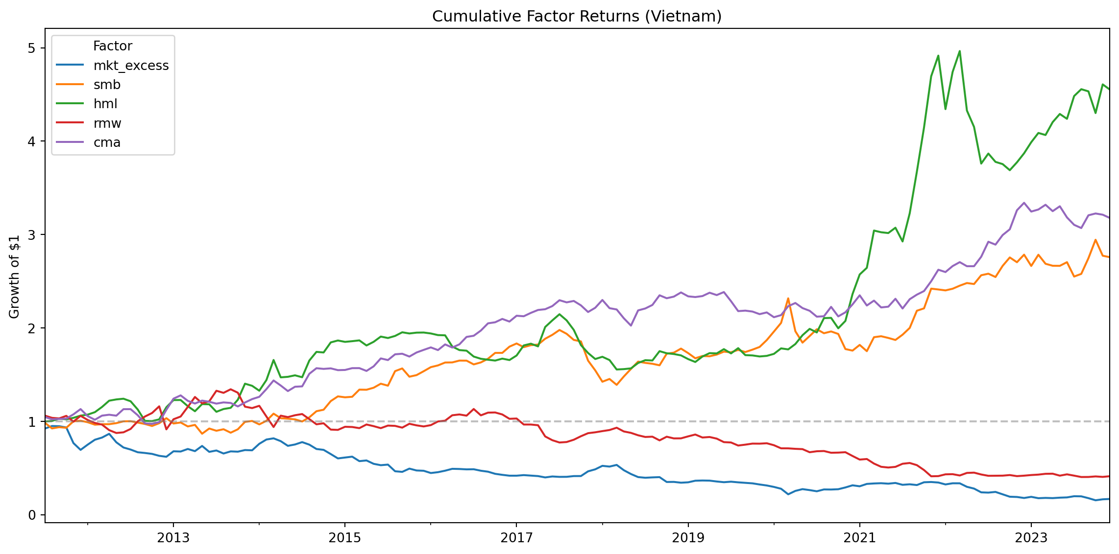
17.8.3 Comparing Monthly and Daily Factors
We verify consistency between monthly and daily factors by computing correlations.
# Aggregate daily factors to monthly for comparison
factors_daily_monthly = (factors_ff5_daily
    .assign(year_month=lambda x: x["date"].dt.to_period("M"))
    .groupby("year_month")
    [["mkt_excess", "smb", "hml", "rmw", "cma"]]
    .sum()  # Sum daily returns to get monthly
    .reset_index()
)

# Merge with actual monthly factors
comparison = (factors_ff5_monthly
    .assign(year_month=lambda x: x["date"].dt.to_period("M"))
    .merge(
        factors_daily_monthly,
        on="year_month",
        suffixes=("_monthly", "_daily")
    )
)

# Correlations
for factor in ["mkt_excess", "smb", "hml", "rmw", "cma"]:
    corr = comparison[f"{factor}_monthly"].corr(comparison[f"{factor}_daily"])
    print(f"{factor}: Monthly-Daily correlation = {corr:.4f}")
mkt_excess: Monthly-Daily correlation = 0.9980
smb: Monthly-Daily correlation = 0.9950
hml: Monthly-Daily correlation = 0.9948
rmw: Monthly-Daily correlation = 0.9929
cma: Monthly-Daily correlation = 0.988417.9 Key Takeaways
Factor Models Explained: The Fama-French three-factor model adds size (SMB) and value (HML) factors to the CAPM, while the five-factor model further includes profitability (RMW) and investment (CMA) factors.
Construction Methodology: Factors are constructed through double-sorted portfolios with careful attention to timing. Portfolios are formed in July using accounting data from the prior fiscal year to ensure information was publicly available.
Independent vs. Dependent Sorts: The three-factor model uses independent sorts on size and book-to-market, creating a 2×3 grid. The five-factor model uses dependent sorts where characteristics are sorted within size groups.
Value-Weighted Returns: Portfolio returns are computed using value-weighting with lagged market capitalization to avoid look-ahead bias.
Daily Factors: Daily factors use the same annual portfolio assignments but compute returns at daily frequency, enabling higher-frequency applications like daily beta estimation.
Market Factor: The market factor is computed independently as the value-weighted return of all stocks minus the risk-free rate.
Validation: Factor quality can be assessed through characteristic monotonicity, portfolio diversification, cumulative returns, and consistency between daily and monthly frequencies.
Vietnamese Market Adaptation: While following the original Fama-French methodology, we adapt for Vietnamese market characteristics including VAS accounting standards, reporting timelines, and currency units.