Reading the output: interpretation, edge cases and decisions

The tour vignette shows how to call the package. This one is about what comes back: what each number means, what to conclude from it, what to write in the paper, and what the output looks like in the situations that confuse people – an unbounded set, a breakdown point of zero or infinity, a large Oster $\delta$ next to a small sign-change $\delta$. It is written for the author who has to defend the analysis and for the referee who has to judge it.

Most examples use simulated data in which the omitted variable exists and is simply hidden from the analysis, so you can see the analysis get it right, and see what it looks like when a conclusion is genuinely fragile. One section uses the bundled BFG (2020) data for a real case.

# A world with six observed covariates w1..w6 and one omitted variable u.
# `beta` is the true effect of x; pi2 and g2 are u's effects on x and y.
# The seed is set by the caller rather than inside here, so that calling
# this does not reach into the session's random stream behind your back.
make_world <- function(beta, pi2, g2, pi1 = rep(0.6, 6), sy = 1,
                       n = 2000) {
    w <- matrix(rnorm(n * 6), n, 6, dimnames = list(NULL, paste0("w", 1:6)))
    u <- 0.3 * w[, 1] + rnorm(n)
    x <- w %*% pi1 + pi2 * u + rnorm(n)
    y <- beta * x + w %*% rep(c(0.4, -0.3), 3) + g2 * u + rnorm(n) * sy
    d <- data.frame(y = as.numeric(y), x = as.numeric(x), w)
    d$u <- u          # kept only so we can check the truth; never used
    d
}
w1   <- paste0("w", 1:6)
form <- y ~ x + w1 + w2 + w3 + w4 + w5 + w6
truth <- function(d) unname(coef(lm(update(form, . ~ . + u), d))["x"])

The numbers, and what each one means

Where it appears	Name	What it is	How to read it
header, $dgp$beta_med	$\beta_{\text{med}}$	the coefficient on $X$ from the regression you can run	the estimate under “no selection on unobservables”
header, $breakdown	breakdown point $\bar r_X^{bp}$	the smallest $\bar r_X$ at which the hypothesis (default: the sign of $\beta_{\text{med}}$) can fail	an unobservable would need to move $X$ at least this much, relative to the calibration covariates, to overturn the conclusion
calibrate_rho()	$\rho_k$	how much covariate $k$ moves $X$ relative to the other calibration covariates	a reference scale for $\bar r_X$: the breakdown point is judged against these
$results	identified set $[\beta_{\min}, \beta_{\max}]$	every $\beta_{\text{long}}$ consistent with the data and the sensitivity parameters	the range of effects you cannot rule out at that level of selection
-Inf, +Inf in $results	unbounded set	the sensitivity parameters no longer restrict $\beta_{\text{long}}$	beyond this $\bar r_X$ the data say nothing; see rmax below
direction = "rybar"	$\bar r_Y^{bp}(\bar r_X)$	the largest effect of the unobservable on $Y$ the conclusion survives, given its effect on $X$	the breakdown frontier; Inf means no outcome effect can overturn it at that $\bar r_X$
analysis = "oster"	$\delta^{bp}$	Oster’s relative-selection coefficient at which the hypothesis fails	$|\delta| = 1$ is “as much selection on unobservables as on observables”; the default sign-change value never exceeds 1 (Case 8)
regsen_boot()	confidence interval	sampling uncertainty in the breakdown point	the breakdown point is an estimate; report it with this

Two facts about the DMP scale that make reading easier:

1. $\bar r_X = 1$ means the omitted variable matters as much for the treatment as all the calibration covariates taken together. A breakdown point above 1 is therefore very robust; one near 0 is not.
2. With cbar = 1 and rybar = Inf, the identified set becomes unbounded at exactly $r_{\max} = \sqrt{1 - R^2(X \sim W_1 \mid W_0)}$. The breakdown point can never exceed $r_{\max}$ in that case, so the comparison “breakdown point versus $\rho_k$” is the informative one; do not read a breakdown point as robust just because it is a large fraction of $r_{\max}$.

The decision path

Having run regsen_bounds() and calibrate_rho(), the question is whether the breakdown point is large relative to what the observed covariates do. DMP’s proposal, and the one we recommend, is:

Breakdown point $\bar r_X^{bp}$	Reading	What to write
above every $\rho_k$	robust	“an unobservable would have to be more important for $X$ than any of the calibration covariates”
above most $\rho_k$, below the largest	moderately robust	name the covariates it does not beat; argue whether an unobservable that important is plausible
below most $\rho_k$	fragile	“an unobservable as important as [a minor covariate] would overturn the sign”
$0$	the hypothesis already fails at $\beta_{\text{med}}$	the point estimate is on the wrong side; sensitivity analysis is not the question
Inf (only with finite rybar)	robust to any selection on $X$	“no amount of selection on the treatment overturns the conclusion once the unobservable’s effect on the outcome is capped at $\bar r_Y$”

Then, in the paper, pair the breakdown point with (i) the $\rho_k$ it is compared to, (ii) its bootstrap interval, and (iii) the choice of calibration set. Those three are what a referee will ask about.

Case 1: a robust conclusion

The true effect is 1; the omitted variable is modest.

set.seed(11)
d <- make_world(beta = 1, pi2 = 0.2, g2 = 0.3, sy = 0.6)
res <- regsen_bounds(form, d, compare = w1, cbar = 1)
rho <- calibrate_rho(form, d, compare = w1)
res$breakdown
#> [1] 0.5135717
rho
#>   variable      rho
#> 1       w1 48.66144
#> 4       w4 46.23054
#> 5       w5 45.37811
#> 2       w2 43.34468
#> 6       w6 43.19672
#> 3       w3 39.38136

The breakdown point is 0.514, and every $\rho_k$ is below it: an unobservable would have to move $X$ more than any single observed covariate does, relative to the others, before the sign of the effect came into doubt. (Recall the $\rho_k$ are printed as percentages; 49% means $\rho_k = 0.49$.) The identified set stays on one side of zero all the way there:

plot(res, xline = res$breakdown)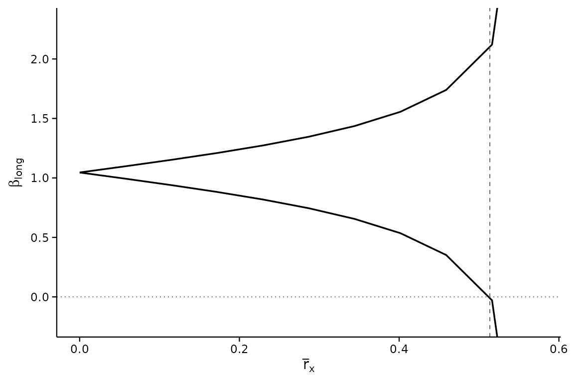

Whether that is “robust enough” is an argument, not a computation: the analysis says how important an omitted variable must be, and the author must say why one that important is implausible. Here we know the truth – the true $\beta$ is 0.985 – and the conclusion is right.

What to write. “The sign of the effect survives any omitted variable whose influence on the treatment, relative to the calibration covariates, is below $\bar r_X = 0.51$. For comparison, the most important calibration covariate has $\rho_k = 0.49$ (Table X); an unobservable would have to matter more for the treatment than any of them.”

Case 2: a fragile conclusion

Here the true effect is zero. The medium regression sees a positive coefficient only because the omitted variable pushes $X$ and $Y$ the same way.

set.seed(12)
d <- make_world(beta = 0, pi2 = 0.8, g2 = 0.8)
res <- regsen_bounds(form, d, compare = w1, cbar = 1)
rho <- calibrate_rho(form, d, compare = w1)
c(beta_med = res$dgp$beta_med, breakdown = res$breakdown)
#>  beta_med breakdown 
#> 0.4110880 0.3176581
range(rho$rho) / 100
#> [1] 0.3762124 0.6526950

The medium coefficient is 0.41 and the naive reading would call it a positive effect. But the breakdown point is 0.32, below every $\rho_k$: an omitted variable less important for the treatment than the least important observed covariate would already be enough to overturn the sign. That is the analysis working as intended – the true effect is 0.02.

plot(res, xline = res$breakdown)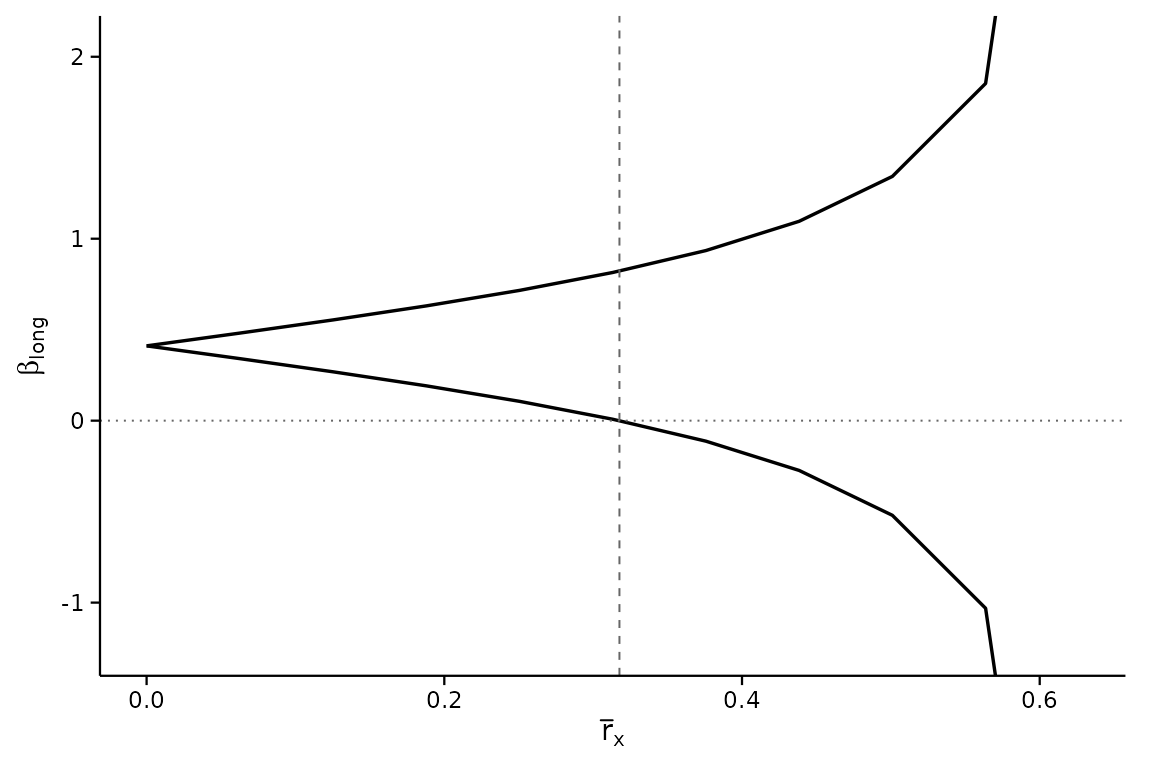

What to write. Do not write “the effect is robust to omitted variable bias.” Write what the number says: “the sign is overturned by an omitted variable with $\bar r_X = 0.32$, less than the contribution of any single calibration covariate,” and let the reader weigh it. If the paper’s claim depends on this coefficient, the honest conclusion is that the data do not establish its sign.

Case 3: a breakdown point of zero

A breakdown point of exactly 0 is not a computation failure. It says the hypothesis is already false at $\bar r_X = 0$, i.e. at $\beta_{\text{med}}$ itself.

set.seed(11)
d <- make_world(beta = 1, pi2 = 0.2, g2 = 0.3, sy = 0.6)
regsen_breakdown(form, d, compare = w1, beta = bnd_lb(2))$results
#>   index breakdown
#> 1     1         0

Testing “$\beta > 2$” when $\beta_{\text{med}} \approx 1$ gives 0: no sensitivity analysis is needed to reject a hypothesis the point estimate already contradicts. The same happens with the default sign hypothesis when the coefficient is on the “wrong” side. Check the Hypothesis: line of the print and res$dgp$beta_med before reading anything else.

Case 4: the set is unbounded early – a weak calibration set

DMP measure the omitted variable against the calibration covariates. If those covariates explain little of the treatment, the yardstick is short and the identified set blows up at a small $\bar r_X$.

set.seed(13)
d <- make_world(beta = 1, pi2 = 0.5, g2 = 0.5, pi1 = rep(0.08, 6))
res <- regsen_bounds(form, d, compare = w1, cbar = 1)
r2 <- res$dgp$covwx_norm_sq / res$dgp$var_x        # R2 of X on W1
c(R2_x_on_w1 = r2, rmax = sqrt(1 - r2), breakdown = res$breakdown)
#> R2_x_on_w1       rmax  breakdown 
#> 0.05820871 0.97045932 0.95321387
calibrate_rho(form, d, compare = w1)
#>   variable        rho
#> 1       w1 118.233328
#> 3       w3  43.504387
#> 5       w5  37.841128
#> 4       w4  32.835219
#> 6       w6  25.683294
#> 2       w2   7.117709

Two things to notice. $R^2(X \sim W_1)$ is only 0.06, so $r_{\max} = \sqrt{1 - 0.06} = 0.97$ and the breakdown point, 0.95, sits close to it. That looks impressive until you see the $\rho_k$: they are all over the place, because when the covariates barely move $X$ their relative contributions are dominated by noise. A breakdown point of 0.95 against a covariate with $\rho_k = 1.18$ is not robust.

What to do. This is the situation in which the choice of calibration set matters most. Move the covariates that genuinely predict the treatment into compare and leave nuisance controls in $W_0$ (see the next case). If nothing observed predicts the treatment, DMP’s analysis has little to calibrate against, and the paper should say so rather than report a breakdown point near $r_{\max}$.

Case 5: which covariates go in compare

The bundled BFG (2020) data has ten geographic covariates and state fixed effects. DMP calibrate against geography and partial out the fixed effects, and the difference is not cosmetic:

data(bfg2020)
bfg2020$statea <- factor(bfg2020$statea)
geo <- c("log_area_2010", "lat", "lon", "temp_mean", "rain_mean",
         "elev_mean", "d_coa", "d_riv", "d_lak", "ave_gyi")
bform <- reformulate(c("tye_tfe890_500kNI_100_l6", geo, "statea"),
                     response = "avgrep2000to2016")

bp_geo <- regsen_bounds(bform, bfg2020, compare = geo, cbar = 1)$breakdown
bp_all <- regsen_bounds(bform, bfg2020, cbar = 1)$breakdown  # FE in W1 too
c(geography_only = bp_geo, geography_and_state_FE = bp_all)
#>         geography_only geography_and_state_FE 
#>              0.8035643              0.2909420

With the fixed effects in the calibration set the breakdown point falls to 0.29. Fixed effects soak up a great deal of the variation in the treatment, so measuring an unobservable against “geography plus 48 state dummies” changes the meaning of $\bar r_X$ entirely – and the $\rho_k$ of a single dummy is not a quantity anyone can reason about. The rule: compare holds the covariates an omitted variable would plausibly resemble; everything else is a control.

A related mistake is to compare breakdown points across specifications with different calibration sets. $\bar r_X$ is relative to $W_1$; change $W_1$ and you have changed the unit.

Case 6: what cbar does, and when it matters

cbar caps how much of the omitted variable the calibration covariates already explain – how endogenous the controls are. The default cbar = 1 imposes nothing. Lowering it can only shrink the identified set, but it binds only once $\bar r_X$ exceeds it:

set.seed(11)
d <- make_world(beta = 1, pi2 = 0.2, g2 = 0.3, sy = 0.6)
regsen_breakdown(form, d, compare = w1, cbar = c(0, 0.25, 0.5, 0.75, 1))$results
#>   index breakdown
#> 1  0.00 0.5985359
#> 2  0.25 0.5354206
#> 3  0.50 0.5136354
#> 4  0.75 0.5135717
#> 5  1.00 0.5135717

The breakdown point is the same for every cbar at or above it. So if you report a breakdown point of, say, 0.5 under cbar = 1, an assertion that the controls are exogenous (cbar = 0) would raise it, but an assertion that they are “not more than 80% endogenous” (cbar = 0.8) would not change it at all. Report cbar = 1 unless you have an argument for less, and if you do, show the sweep so the reader sees whether it mattered.

clow is the other end of the same assumption: setting it above zero asserts the controls are at least that endogenous, which also narrows the set. Use it only when the paper’s own argument implies it.

Case 7: bounding the effect on the outcome too

With rybar = Inf the omitted variable may matter arbitrarily much for $Y$. Capping that with a finite rybar shrinks the set, and can make the breakdown point infinite: no amount of selection on the treatment overturns the sign once the outcome channel is capped tightly enough.

set.seed(11)
d <- make_world(beta = 1, pi2 = 0.2, g2 = 0.3, sy = 0.6)
sapply(c(Inf, 2, 1, 0.5), function(ry) {
    regsen_breakdown(form, d, compare = w1, cbar = 1, rybar = ry)$results$breakdown
})
#> [1] 0.5135717 0.5135895 0.5135895       Inf

Read Inf here as a statement about the frontier, not a bug: at rybar = 0.5 the conclusion survives every $\bar r_X$. The other direction of the same frontier reports, for each $\bar r_X$, how large $\bar r_Y$ may be:

fr <- regsen_breakdown(form, d, compare = w1, cbar = 1,
                       direction = "rybar", rxbar = c(0.25, 0.5, 1, 2))
fr$results
#>   index breakdown
#> 1  0.25       Inf
#> 2  0.50       Inf
#> 3  1.00 0.5099323
#> 4  2.00 0.5099323

What to write. The common-impact case rybar_expr = function(r) r (the unobservable matters equally for treatment and outcome) is the one-number summary DMP report alongside the rybar = Inf breakdown point; report both. Say explicitly which rybar a reported breakdown point assumes, since a finite rybar is an extra assumption and a referee will want it justified.

Case 8: Oster’s $\delta$, and why a large one is not enough

Oster’s $\delta$ is the ratio of selection on unobservables to selection on observables, and the convention treats $|\delta| \ge 1$ as implausible. Masten and Poirier (2026) show that “Oster’s $\delta$” names two different numbers, and give them names:

• the explain away breakdown point: the $\delta$ at which $\beta$ reaches zero. This is what psacalc computes and what published work reports.
• the sign change breakdown point: the smallest $|\delta|$ at which some value of the opposite sign enters the identified set.

The second is often far smaller. In the example Masten and Poirier open with, the explain away value is $-32$ and the sign change value is $0.586$; on the frontier data of this package it is $-23.3$ against $0.974$.

set.seed(12)
d <- make_world(beta = 0, pi2 = 0.8, g2 = 0.8)
d_eq   <- regsen_breakdown(form, d, compare = w1, analysis = "oster",
                           r2long = 1, beta = bnd_eq(0))$results$breakdown
d_sign <- regsen_breakdown(form, d, compare = w1, analysis = "oster",
                           r2long = 1)$results$breakdown
c(explain_away = d_eq, sign_change = d_sign)
#> explain_away  sign_change 
#>    0.8897076    0.6775042

Both are on the fragile world of Case 2. The sign change breakdown is the one that answers “could the conclusion be wrong?”, and it is the one to report; regsen_breakdown() computes it by default. The two coincide only when the identified set passes through zero as $|\delta|$ grows, which is not guaranteed – the set can jump across zero as a branch of Oster’s cubic diverges, which is exactly what happens near $\delta = 1$:

o <- regsen_bounds(form, d, compare = w1, analysis = "oster",
                   delta = seq(-2, 2, 0.02), r2long = 1)
plot(o, ylim = c(-3, 3))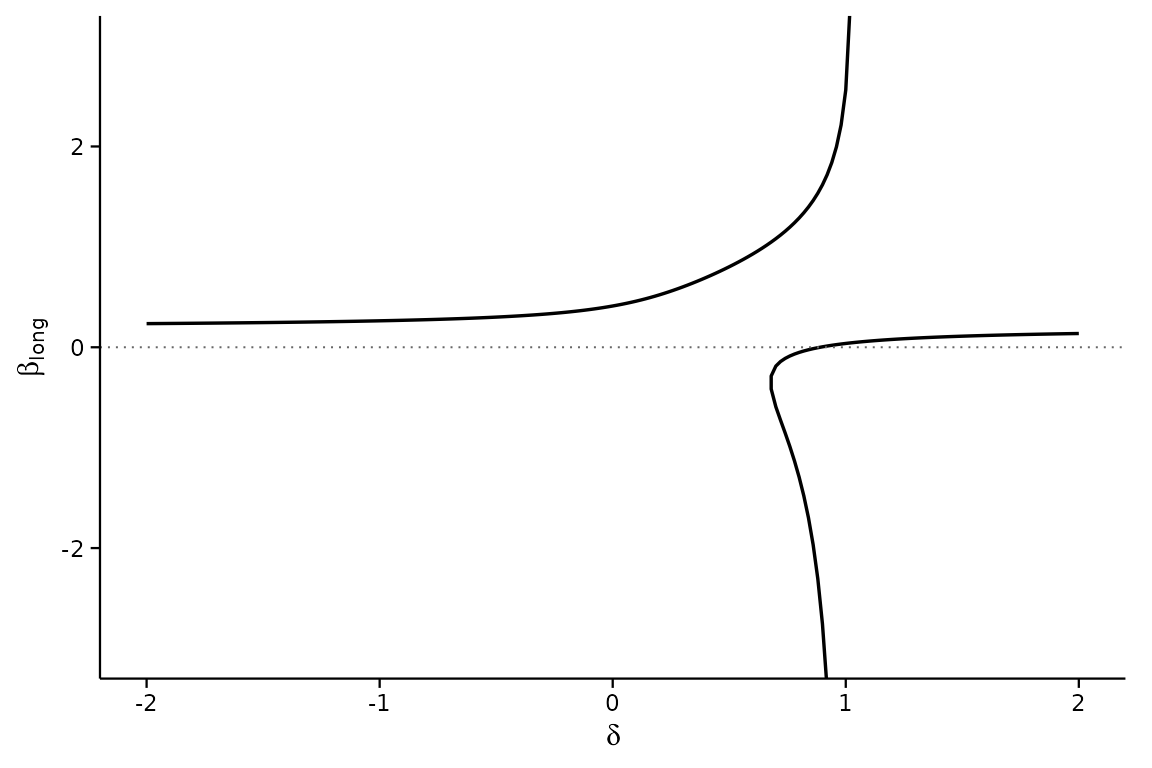

One consequence is a hard ceiling. Masten and Poirier’s Theorem 2 proves that the sign change breakdown point can never exceed one, so a sign conclusion is never “robust” by the $|\delta| > 1$ criterion, whatever the explain away number says. regsen_breakdown() reports the sign change value capped at one for that reason: a printed 1 means the sign survives every $|\delta|$ below the cutoff, not that a solution was found at exactly one. The only way past the ceiling is to add an assumption, which is what maxovb does (Section 3.2 of Masten and Poirier): a bound on how far the coefficient can move rules out the sign change the theorem otherwise guarantees, and the reported value can then exceed one.

Two further conventions to state in the paper: the value of r2long (Oster’s $R_{\max}$; 1 is the conservative choice, $1.3 \times R^2_{\text{med}}$ her rule of thumb), and whether maxovb was used to cap the bias.

Case 9: the bootstrap interval

The breakdown point is a statistic. Its bootstrap interval is what makes the comparison with $\rho_k$ honest:

bb <- regsen_boot(bform, bfg2020, compare = geo, cbar = 1,
                  R = 199, cluster = "km_grid_cel_code", seed = 1,
                  show_progress = FALSE)
bb
#> Bootstrap confidence interval for the breakdown point
#> ------------------------------------------------------------
#>   R                  : 199
#>   Cluster bootstrap  : km_grid_cel_code
#>   Interval           : BCa
#>   Bias corr. (z0)    : 1.1233
#>   Acceleration       : -0.0008
#>   Confidence level   : 95%
#>   Point estimate     : 0.8036
#>   95% CI            : [0.7465, 0.9025]
#>   (An endpoint is an extreme replicate; raise R)
#>   95% CI (percentile): [0.4997, 0.8612]

Read the BCa interval as the default; the percentile one is printed for comparison. Here the two differ a good deal: z0 is large, meaning most cluster resamples gave a breakdown point below the full-sample one, and BCa shifts the quantiles it reads to correct for that. Three things the print can add:

• “BCa unavailable; showing percentile” – the bias or acceleration constant was undefined (every replicate on one side of the estimate, or a degenerate jackknife). Raise R, or report the percentile interval.
• “An endpoint is an extreme replicate; raise R” – the adjusted quantile fell on the smallest or largest replicate. 199 is a small R for a paper; 999 or 1999 is usual.
• “Infinite replicates” – on some resamples the hypothesis survived every value of the parameter (this arises with finite rybar). They are counted as $+\infty$ in the interval, so an upper endpoint of Inf is a result, not an error.

Cluster at the level the paper’s standard errors are clustered at. The jackknife behind BCa then runs over clusters rather than rows.

What to write. “The breakdown point is 0.80 (95% cluster-bootstrap BCa interval [$\cdot$, $\cdot$], $R = 1999$).”

Case 10: several treatments at once

When the paper has several coefficients of interest, regsen_multi() gives each its breakdown point in the same specification, so they can be compared:

regsen_multi(bform, bfg2020,
             treatments = c("tye_tfe890_500kNI_100_l6", "lat", "temp_mean"),
             compare = geo, cbar = 1)
#> 
#> Sensitivity across treatments
#> ------------------------------------------------------------
#>                 treatment estimate breakdown     n
#>  tye_tfe890_500kNI_100_l6    2.055    0.8036  2036
#>                       lat    2.265   0.03622  2036
#>                 temp_mean    1.627   0.02502  2036

Each row promotes one variable to the treatment and keeps every other term as a control, so the rows are comparable. A row with a near-zero breakdown point is a coefficient whose sign the data do not establish.

Common mistakes

• Reading a breakdown point as a probability. It is a threshold on a relative magnitude, not a probability that the conclusion is wrong.
• Reporting the breakdown point without $\rho_k$. On its own the number has no scale. Always table the $\rho_k$ next to it.
• Reporting it without an interval. See Case 9.
• Putting fixed effects in compare. See Case 5.
• Comparing breakdown points across specifications with different calibration sets. The unit changes with $W_1$.
• Reading a plateau in the plot as “the bound levels off.” Bounds that leave the panel are unbounded; the package draws them exiting the plot rather than flat along the edge for this reason.
• Mixing up the two Oster breakdown points. The explain away value (reaches zero) is not the sign change value (flips the sign), and only the second bears on whether the sign could be wrong (Case 8).
• Treating rybar as free. A finite rybar is a substantive assumption about the outcome equation. State it.

A reporting checklist

For a sensitivity analysis a referee can evaluate, the paper needs:

1. The specification: outcome, treatment, which covariates are in the calibration set $W_1$ and which are controls $W_0$, and why.
2. The breakdown point under the default (cbar = 1, rybar = Inf) and under common impact (rybar = rxbar), with bootstrap intervals.
3. The calibration table: $\rho_k$ for every $W_1$ covariate (calibrate_rho()), and optionally their pairwise partial $R^2$ (calibrate_partial_r2()).
4. One figure: the identified set against $\bar r_X$ with the breakdown point marked (plot(res, xline = res$breakdown)), or the frontier.
5. If Oster’s $\delta$ is reported: the sign-change breakdown, the r2long used, and whether maxovb was imposed.
6. A sentence saying what magnitude of omitted variable the conclusion is robust to, in words a reader can weigh against the setting.

regsen_table(res, notes = TRUE) writes the specification note for a table; regsen_glance(res) collects the headline numbers in one row.

References

• Diegert, P., Masten, M., and Poirier, A. (2026). Assessing Omitted Variable Bias when the Controls are Endogenous. arXiv:2206.02303.
• Oster, E. (2019). Unobservable Selection and Coefficient Stability: Theory and Evidence. JBES 37(2), 187–204.
• Masten, M., and Poirier, A. (2026). The Effect of Omitted Variables on the Sign of Regression Coefficients. AER 116(7), 2685–2710.