
Side by side with the published figures
Source:vignettes/articles/figure-comparison.Rmd
figure-comparison.RmdA replication that only reports numbers asks you to trust that the figures line up too. This page puts them next to each other.
The published panels are reproduced from Diegert, Masten and
Poirier (2026), Assessing Omitted Variable
Bias when the Controls are Endogenous (arXiv:2206.02303v6) and
Masten and Poirier (2026), The Effect of Omitted
Variables on the Sign of Regression Coefficients
(arXiv:2208.00552v5), for the purpose of comparison. Copyright rests
with the authors. The panels beneath each one are produced by this
package from the bundled bfg2020 data, by the code shown
with them.
This page is part of the website only. It is excluded from the package tarball, so the reproduced figures are not redistributed on CRAN.
Figure 1, left panel
Bounds on against at . Solid lines leave unrestricted; dashed lines impose . The marks on the zero line are the Table 4 calibration values.

regsensitivity
rx <- seq(0, 1.4, length.out = 300)
solid  <- regsen_bounds(form, bfg2020, compare = w1, cbar = 1, rxbar = rx)
dashed <- regsen_bounds(form, bfg2020, compare = w1, cbar = 1, rxbar = rx,
                         rybar_expr = function(r) r)

a <- as.data.frame(solid);  a$spec <- "rybar = Inf"
b <- as.data.frame(dashed); b$spec <- "rybar = rxbar"
df <- rbind(a[, c("rxbar", "bmin", "bmax", "spec")],
            b[, c("rxbar", "bmin", "bmax", "spec")])
df$bmin[!is.finite(df$bmin)] <- NA
df$bmax[!is.finite(df$bmax)] <- NA
ticks <- calibrate_rho(form, bfg2020, compare = w1)$rho / 100

ggplot(df, aes(x = rxbar, linetype = spec)) +
    geom_hline(yintercept = 0, colour = "grey30", linewidth = 0.3,
                linetype = "dotted") +
    geom_line(aes(y = bmin), linewidth = 0.5, na.rm = TRUE) +
    geom_line(aes(y = bmax), linewidth = 0.5, na.rm = TRUE) +
    annotate("segment", x = ticks, xend = ticks, y = -0.25, yend = 0.25,
              linewidth = 0.35, colour = "black") +
    scale_linetype_manual(values = c("rybar = Inf"   = "solid",
                                     "rybar = rxbar" = "dashed")) +
    scale_x_continuous(breaks = seq(0, 1.4, 0.2)) +
    scale_y_continuous(breaks = seq(-2, 6, 2)) +
    coord_cartesian(xlim = c(0, 1.5), ylim = c(-3.2, 7.2)) +
    labs(x = expression(bar(r)[X]), y = expression(beta[long]),
         linetype = NULL) +
    theme_regsen(base_size = 10) +
    theme(legend.position = "none")
The two curves cross zero at the paper’s two breakdown points:
c(`rybar = Inf`   = abs(solid$breakdown),    # paper: 0.804
  `rybar = rxbar` = abs(dashed$breakdown))   # paper: 0.959 (96% in prose)
#>   rybar = Inf rybar = rxbar
#>     0.8035643     0.9583504
Both bounds go infinite at under the dashed specification, and just below 1 under the solid one, which is where both curves leave the panel in the published figure too.
Figure 1, right panel
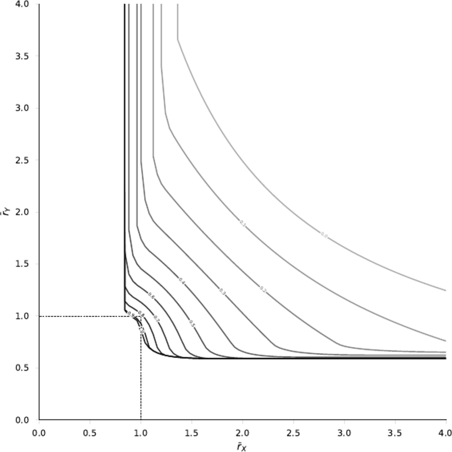
The breakdown frontier in space, one curve per .
regsensitivity
# The frontier in the rybar direction: one solve per rxbar, parallelised
# across the grid (forking is unavailable on Windows, hence the fallback).
frontier <- function(cbar, rxs, w = w1) {
    cores <- if (.Platform$OS.type == "windows") 1L else
        min(4L, max(1L, parallel::detectCores(), na.rm = TRUE))
    res <- parallel::mclapply(rxs, function(rx) {
        r <- regsen_breakdown(form, bfg2020, compare = w, cbar = cbar,
                               direction = "rybar", rxbar = rx)
        r$results$breakdown[1]
    }, mc.cores = cores)
    ry <- vapply(res, function(z) if (is.numeric(z)) z else NA_real_,
                 numeric(1))
    data.frame(rxbar = rxs, rybar = ry, cbar = factor(cbar))
}
# Dense through the bend; the flat arm to the right needs only anchors.
rxs <- c(seq(0.7, 2, by = 0.05), 2.25, 2.5, 3, 3.5, 4)
fr  <- do.call(rbind, lapply(c(1, 0.9, 0.75, 0.5), frontier, rxs = rxs))

# Below its breakdown point in rxbar the conclusion survives every rybar,
# so the frontier is +Inf there: send those points off the top of the
# panel and let coord_cartesian clip, which is the vertical arm.
fr$rybar[!is.finite(fr$rybar)] <- 40

# As in the paper: thick black is cbar = 1; the greys are 0.9, 0.75,
# and 0.5, moving outward. Dotted guides mark rxbar = rybar = 1.
frontier_plot <- function(fr) {
    ggplot(fr, aes(x = rxbar, y = rybar, group = cbar)) +
        geom_hline(yintercept = 1, colour = "grey60", linewidth = 0.3,
                    linetype = "dotted") +
        geom_vline(xintercept = 1, colour = "grey60", linewidth = 0.3,
                    linetype = "dotted") +
        geom_line(aes(linewidth = cbar == "1", colour = cbar == "1"),
                   na.rm = TRUE) +
        scale_linewidth_manual(values = c(`TRUE` = 0.9, `FALSE` = 0.4),
                                guide = "none") +
        scale_colour_manual(values = c(`TRUE` = "black",
                                        `FALSE` = "grey55"),
                             guide = "none") +
        scale_x_continuous(breaks = seq(0, 4, 0.5)) +
        scale_y_continuous(breaks = seq(0, 4, 0.5)) +
        coord_cartesian(xlim = c(0, 4), ylim = c(0, 4)) +
        labs(x = expression(bar(r)[X]), y = expression(bar(r)[Y])) +
        theme_regsen(base_size = 10)
}
frontier_plot(fr)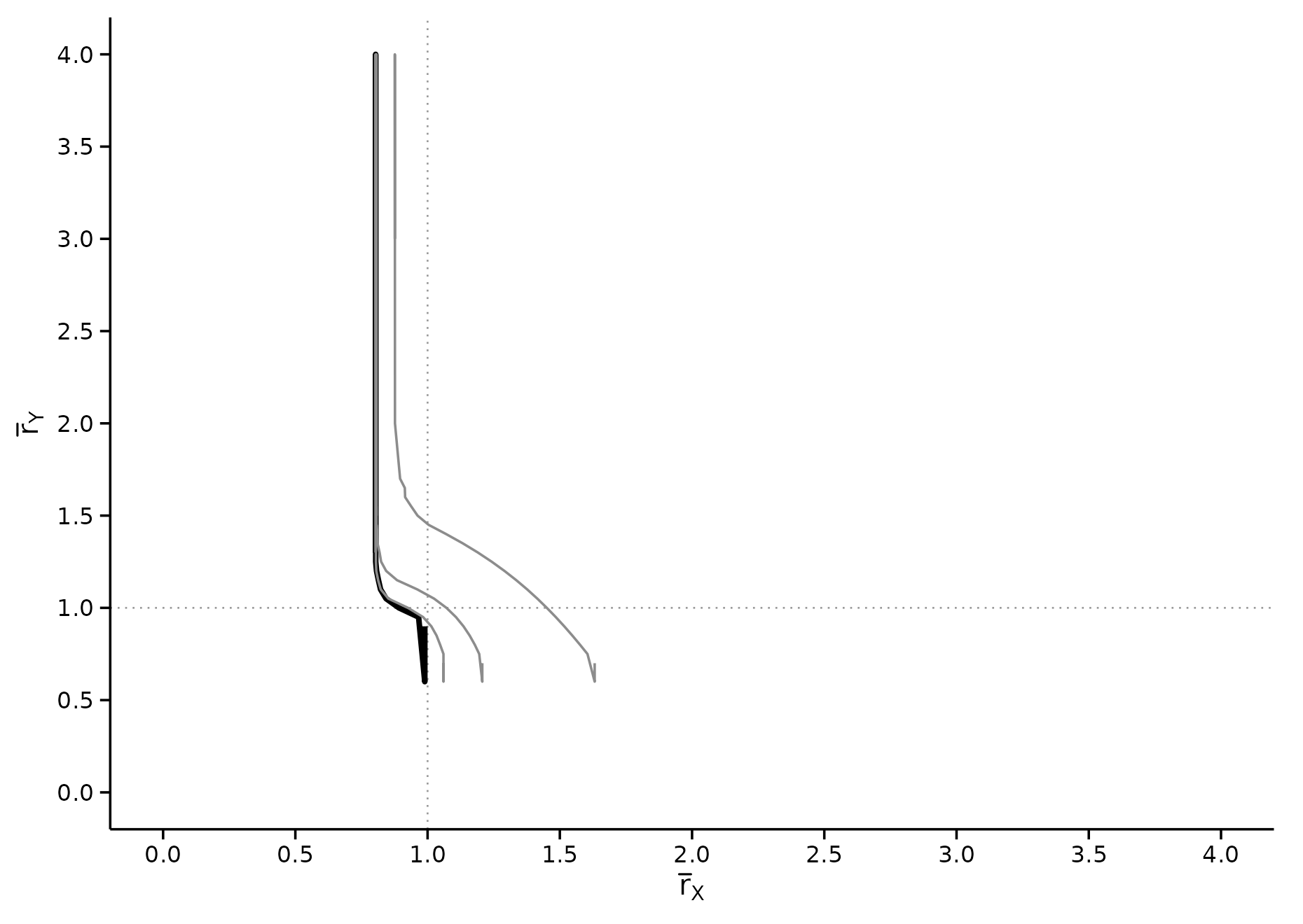
Both arms are here. The vertical one sits at the breakdown point of Table 1, Panel C – each curve approaches as grows – and the horizontal one is the level of below which no amount of selection on the treatment side overturns the sign, which is what the curve flattening onto it means.
The horizontal arm is the part that needed the frontier in the direction. Sweeping and solving for cannot draw it, because along that arm the answer is : every leaves the conclusion standing.
# Far out on the horizontal arm, where the identified set is still
# bounded because rybar is restricted even though rxbar is not.
regsen_bounds(form, bfg2020, compare = w1, cbar = 1,
              rxbar = 2, rybar = 0.6)$results
#>   rxbar rybar cbar        bmin    bmax
#> 1     2   0.6    1 -0.05202383 4.31302

# ... and the rybar frontier at the same rxbar, which is what the curve
# above plots.
regsen_breakdown(form, bfg2020, compare = w1, cbar = 1,
                 direction = "rybar", rxbar = 2)$results
#>   index breakdown
#> 1     2 0.5901671
Figure 3: calibrating with state fixed effects
Figure 3 repeats Figure 1 with the state fixed effects moved into the calibration set. The paper’s point is that is only meaningful relative to the covariates it calibrates against: adding controls with a lot of explanatory power raises selection on observables, so the same data yields a much smaller breakdown point – the paper says it drops from about 80% to about 30%.

regsensitivity
w1_fe <- c(w1, "statea")          # state fixed effects now calibrate too
s3 <- regsen_bounds(form, bfg2020, compare = w1_fe, cbar = 1, rxbar = rx)
d3 <- regsen_bounds(form, bfg2020, compare = w1_fe, cbar = 1, rxbar = rx,
                     rybar_expr = function(r) r)

a3 <- as.data.frame(s3); a3$spec <- "rybar = Inf"
b3 <- as.data.frame(d3); b3$spec <- "rybar = rxbar"
df3 <- rbind(a3[, c("rxbar", "bmin", "bmax", "spec")],
             b3[, c("rxbar", "bmin", "bmax", "spec")])
df3$bmin[!is.finite(df3$bmin)] <- NA
df3$bmax[!is.finite(df3$bmax)] <- NA

ggplot(df3, aes(x = rxbar, linetype = spec)) +
    geom_hline(yintercept = 0, colour = "grey30", linewidth = 0.3,
                linetype = "dotted") +
    geom_line(aes(y = bmin), linewidth = 0.5, na.rm = TRUE) +
    geom_line(aes(y = bmax), linewidth = 0.5, na.rm = TRUE) +
    scale_linetype_manual(values = c("rybar = Inf"   = "solid",
                                     "rybar = rxbar" = "dashed")) +
    # The published Figure 3 panel uses a wider y window than Figure 1,
    # so the reproduction adopts the same one.
    scale_y_continuous(breaks = seq(-5, 10, 5)) +
    coord_cartesian(xlim = c(0, 1.5), ylim = c(-8.5, 14)) +
    labs(x = expression(bar(r)[X]), y = expression(beta[long]),
         linetype = NULL) +
    theme_regsen(base_size = 10) +
    theme(legend.position = "none")
The published Figure 3 also has a right panel: the breakdown frontiers recomputed with the state fixed effects in the calibration set. All of them have shifted inward, the point the paper makes in the surrounding text.
rxs3 <- c(seq(0.25, 2, by = 0.05), 2.25, 2.5, 3, 3.5, 4)
fr3  <- do.call(rbind, lapply(c(1, 0.75), frontier, rxs = rxs3, w = w1_fe))
fr3$rybar[!is.finite(fr3$rybar)] <- 40
frontier_plot(fr3)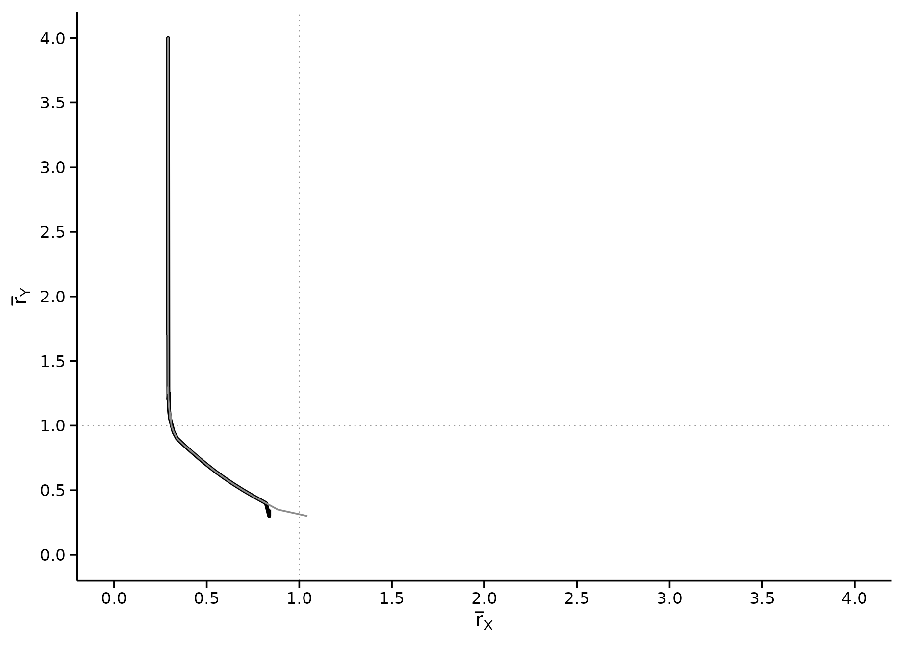
Both arms again, with the vertical one now near 0.29 instead of 0.80 – the inward shift the paper describes.
Masten and Poirier (2026), Figures 1 and 2
These two are built on the authors’ application to Satyanath et al. (2017), which is not bundled with this package, and the paper does not report the moments needed to rebuild the curves – it prints coefficients and breakdown points, but no R-squared values and no variances. A full numerical reproduction would require re-running the regressions on the Satyanath et al. microdata (Harvard Dataverse, doi:10.7910/DVN/EE6I7N). The figures are shown here for structure, next to the stylized illustration in the MP examples vignette.
This is not a numerical reproduction, and it should not be read as one. In the published figure the sign-change breakdown is 0.586 while the explain-away breakdown is – a separation of a factor of 55, which is precisely the asymmetry the figure exists to demonstrate. In constructed data the two quantities come out close together; reproducing the gap needs the actual Satyanath moments, not a plausible-looking substitute.

MP (2026) Figure 2, as published

The structural features do carry over to constructed data: the identified set has at most three solutions at any , and a solution escapes to infinity at , where a second branch enters from the other side and sweeps across zero. Both are visible in the stylized figures in that vignette.
Coverage: every figure in the three papers
| Figure | Status | Reason |
|---|---|---|
| DMP Fig 1 (left) | reproduced | matches on both specifications; crossings 0.8036 / 0.9584 |
| DMP Fig 1 (right) | reproduced | both arms match; the horizontal one is drawn in the rybar direction |
| DMP Fig 2 | not reproducible | outcome ‘Cut Spending on Poor’ is not in the bundled bfg2020 data |
| DMP Fig 3 (left) | reproduced | matches; breakdown falls to 0.2909 against the paper’s ‘about 30%’ |
| DMP Fig 3 (right) | reproduced | matches, shifted inward as in the paper |
| MP Fig 1 | structure only | built on Satyanath et al. (2017); moments not reported in full |
| MP Fig 2 | structure only | as Figure 1 |
| MP Fig S1 | not reproducible | Satyanath et al. (2017) data, not bundled |
| Oster Figs 1, 4-6 | out of scope | meta-analysis over Oster’s hand-collected samples of published papers (Figs 1, 4, 5: the 27-paper coefficient-stability sample; Fig 6: her randomized-trials sample) |
| Oster Fig 2 | out of scope | a Monte Carlo of the bias-adjusted estimator’s sampling distribution, a simulation study rather than an analysis the package performs |
| Oster Fig 3 | out of scope | NLSY-79 validation exercise with a bespoke data construction, not a package analysis |
Every panel this package’s methods can produce from the bundled data is reproduced above, in full: both bounds panels and both frontier panels, each frontier with both of its arms. The rest need data that is not distributed with the package – the full BFG outcome set, or the Satyanath et al. microdata – or, in Oster’s case, are simulation and literature meta-analysis exercises rather than sensitivity analyses of a dataset.