Coming from the Stata package

The reference implementation of these methods is Masten and Poirier’s Stata package, also called regsensitivity. This vignette maps its syntax onto this package, command by command, using the same BFG (2020) data that the Stata vignette uses.

It doubles as a coverage check. Every command in the Stata package’s own vignette (shipped here as inst/stata-reference/vignette.do) appears below with its R equivalent, so a gap would be visible rather than implicit.

data(bfg2020)
bfg2020$statea <- factor(bfg2020$statea)

w1 <- c("log_area_2010", "lat", "lon", "temp_mean", "rain_mean",
        "elev_mean", "d_coa", "d_riv", "d_lak", "ave_gyi")

form <- avgrep2000to2016 ~ tye_tfe890_500kNI_100_l6 +
    log_area_2010 + lat + lon + temp_mean + rain_mean + elev_mean +
    d_coa + d_riv + d_lak + ave_gyi + statea

In Stata the outcome, treatment and controls are positional and the comparison set is named separately:

local y avgrep2000to2016
local x tye_tfe890_500kNI_100_l6
local w1 log_area_2010 lat lon temp_mean rain_mean elev_mean d_coa d_riv d_lak ave_gyi
local w0 i.statea
regsensitivity `y' `x' `w1' `w0', compare(`w1')

In R the same information is a formula plus compare. The first term on the right-hand side is the treatment; everything else is a control.

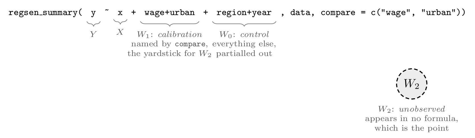
A regsen_summary call with braces under its parts: y is the outcome Y, x is the treatment X, the terms named by compare are the calibration covariates W1, and the remaining right-hand-side terms are the control covariates W0, which are partialled out. A dashed circle stands for the unobserved W2, which appears in no formula.

compare and nocompare are two ways of drawing the same line, and you may give at most one of them: compare names the calibration set $W_1$ , nocompare names its complement $W_0$ . Give neither and every control enters $W_1$ .

Command map

Stata	R
`regsensitivity y x w, compare(w1)`	`regsen_summary(form, data, compare = w1)`
`regsensitivity bounds ...`	`regsen_bounds(form, data, ...)`
`regsensitivity breakdown ...`	`regsen_breakdown(form, data, ...)`
`regsensitivity plot`	`plot(result)`
`compare(w1)`	`compare = w1`
`nocompare(w0)`	`nocompare = w0`
`cbar(0(.2)1)`	`cbar = seq(0, 1, 0.2)`
`rxbar(0 2)`	`rxbar = c(0, 2)`
`rybar(2)`	`rybar = 2`
`rybar(=rxbar)`	`rybar_expr = function(rx) rx`
`beta(0 eq)`	`beta = bnd_eq(0)`
`beta(4 ub)`	`beta = bnd_ub(4)`
`beta(-1(.2)1 lb)`	`beta = bnd_lb(seq(-1, 1, 0.2))`
`beta(sign)`	`beta = "sign"` (the default)
`oster`	`analysis = "oster"`
`delta(-3 3 eq)`	`delta = c(-3, 3)`, `delta_type = "eq"`
`delta(0(.001).999 bound)`	`delta = seq(0, .999, .001)`, `delta_type = "bound"`
`rmax(0(.1)1)`	`r2long = seq(0, 1, 0.1)`
`plot, nolegend`	`plot(res, show_legend = FALSE)`
`plot, yrange(0 6)`	`plot(res, ylim = c(0, 6))`
`plot, ywidth(4)`	`plot(res, ywidth = 4)`
`plot, xline(1)`	`plot(res, xline = 1)`
`e(idset_table)`	`as.data.frame(res)`
`cluster(v)` on the regression	`regsen_boot(..., cluster = "v")`

Two differences are worth flagging rather than burying in the table.

Stata’s numlist syntax 0(.2)1 means “from 0 to 1 in steps of .2”, which is seq(0, 1, 0.2). And Stata stores results in e() matrices retrieved with matrix subscripts; here the results are already a data frame, so as.data.frame(res) gives you the same content directly.

The Stata vignette, translated

Default summary

regsensitivity `y' `x' `w', compare(`w1')

summ <- regsen_summary(form, bfg2020, compare = w1)
summ
#> 
#> === DMP (2026) bounds ===
#> 
#> Regression Sensitivity Analysis ----- Bounds
#> ------------------------------------------------------------------------
#> Analysis:          DMP (2026)
#> Treatment:         tye_tfe890_500kNI_100_l6
#> Outcome:           avgrep2000to2016
#> N (obs):           2036
#> Hypothesis:        Beta > 0
#> Breakdown point:   0.8036
#> 
#> --- Summary statistics ----------------------------------
#>   Beta (short)                  1.9246
#>   Beta (medium)                 2.0548
#>   R2 (short)                    0.0328
#>   R2 (medium)                   0.1051
#>   Var(Y)                      101.7387
#>   Var(X)                        0.9014
#>   Var(X_Residual)               0.8823
#> 
#> --- Results ---------------------------------------------
#>     rxbar rybar   cbar     bmin   bmax
#>         0  +Inf      1   2.0548 2.0548
#>  0.098939  +Inf      1   1.9064 2.2031
#>   0.19788  +Inf      1   1.7535  2.356
#>   0.29682  +Inf      1   1.5906 2.5189
#>   0.39576  +Inf      1   1.4106 2.6989
#>   0.49469  +Inf      1   1.2026 2.9069
#>   0.59363  +Inf      1  0.94779 3.1617
#>   0.69257  +Inf      1  0.60803 3.5015
#>   0.79151  +Inf      1 0.086812 4.0227
#>   0.89045  +Inf      1 -0.99272 5.1022
#>   0.98939  +Inf      1     -Inf   +Inf
#> 
#> === Oster (2019) breakdown ===
#> 
#> Regression Sensitivity Analysis ----- Breakdown Frontier
#> ------------------------------------------------------------------------
#> Analysis:          Oster (2019)
#> Treatment:         tye_tfe890_500kNI_100_l6
#> Outcome:           avgrep2000to2016
#> N (obs):           2036
#> Hypothesis:        Beta > 0
#> 
#> --- Summary statistics ----------------------------------
#>   Beta (short)                  1.9246
#>   Beta (medium)                 2.0548
#>   R2 (short)                    0.0328
#>   R2 (medium)                   0.1051
#>   Var(Y)                      101.7387
#>   Var(X)                        0.9014
#>   Var(X_Residual)               0.8823
#> 
#> --- Results ---------------------------------------------
#>    index breakdown
#>  0.13667   0.97393
#>  0.23667   0.97315
#>  0.33667   0.97232
#>  0.43667   0.97145
#>  0.53667   0.97052
#>  0.63667   0.96954
#>  0.73667    0.9685
#>  0.83667   0.96739
#>  0.93667   0.96622
#>        1   0.96543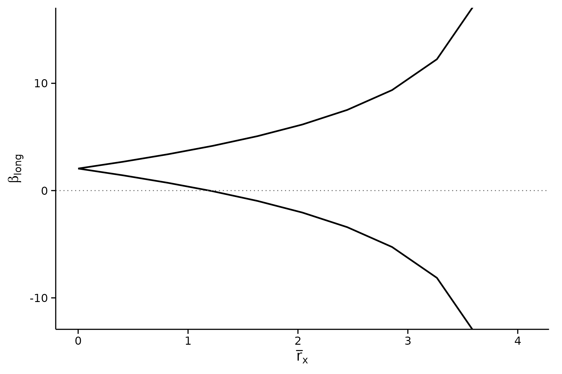

Bounds at a single `cbar`

regsensitivity bounds `y' `x' `w', compare(`w1') cbar(.1)
regsensitivity plot

b1 <- regsen_bounds(form, bfg2020, compare = w1, cbar = 0.1)
plot(b1)

Bounds over a grid of `cbar`

regsensitivity bounds `y' `x' `w', compare(`w1') cbar(0(.2)1)

b2 <- regsen_bounds(form, bfg2020, compare = w1,
                     cbar = seq(0, 1, 0.2))
plot(b2)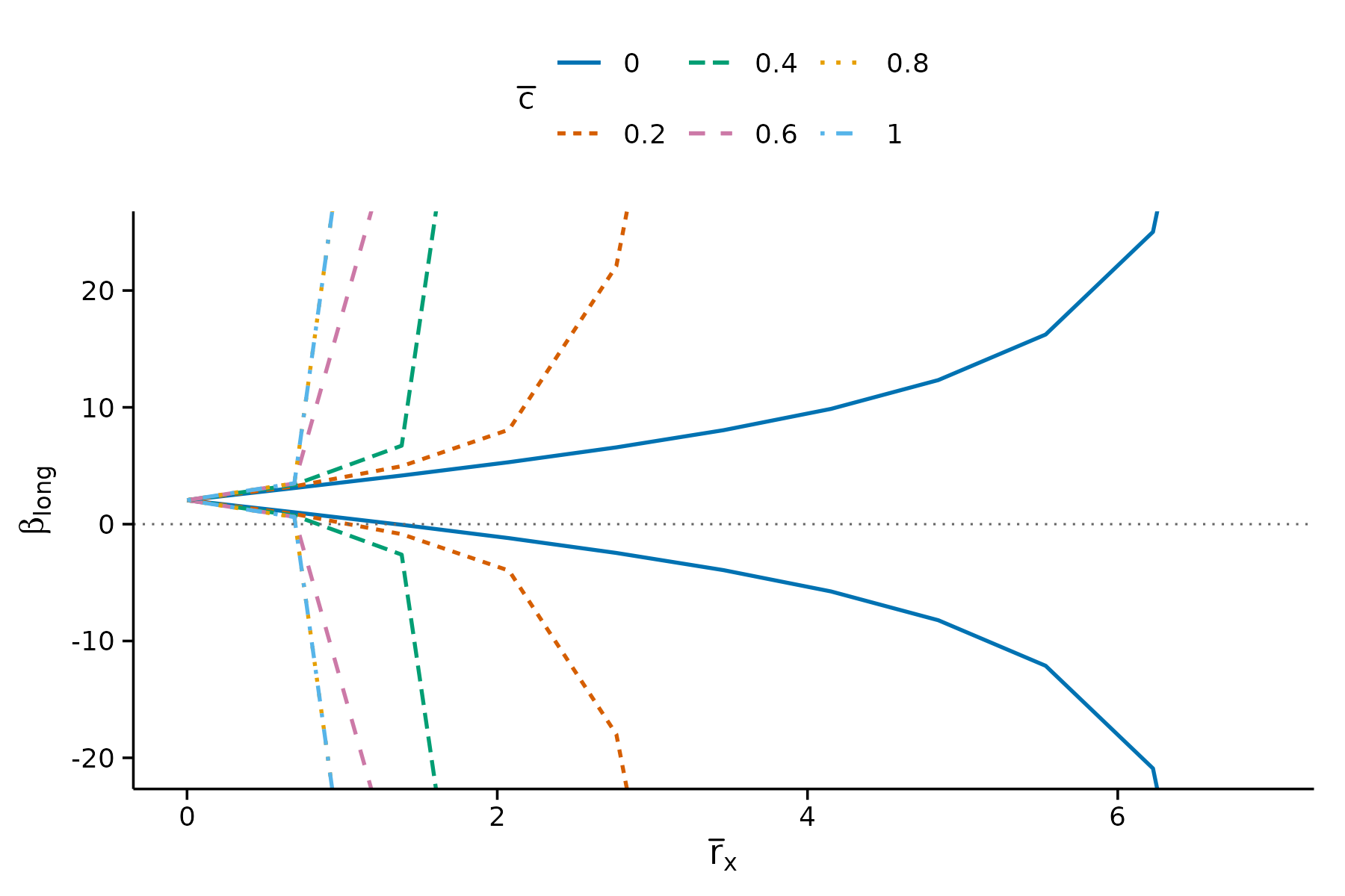

Restricting `rxbar` as well

regsensitivity bounds `y' `x' `w', compare(`w1') cbar(0(.2)1) rxbar(0 2) plot

b3 <- regsen_bounds(form, bfg2020, compare = w1,
                     cbar = seq(0, 1, 0.2), rxbar = c(0, 2))
plot(b3)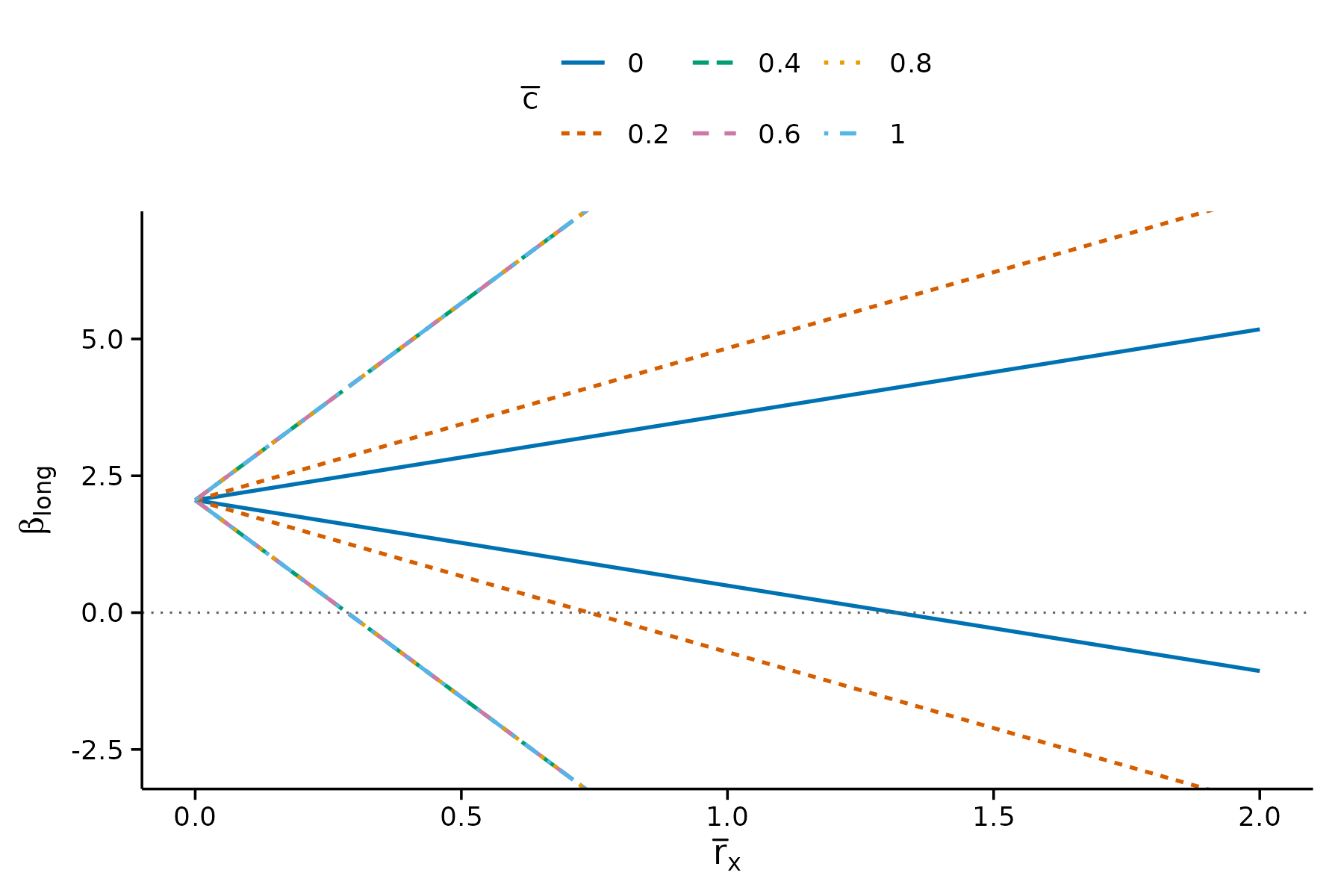

Breakdown frontier

regsensitivity breakdown `y' `x' `w', compare(`w1') cbar(0(.1)1)
regsensitivity plot

bd <- regsen_breakdown(form, bfg2020, compare = w1,
                        cbar = seq(0, 1, 0.1))
plot(bd)

Breakdown for a one-sided hypothesis

regsensitivity breakdown `y' `x' `w', compare(`w1') cbar(0(.1)1) beta(4 ub)

bd_ub <- regsen_breakdown(form, bfg2020, compare = w1,
                           cbar = seq(0, 1, 0.1), beta = bnd_ub(4))
bd_ub
#> 
#> Regression Sensitivity Analysis ----- Breakdown Frontier
#> ------------------------------------------------------------------------
#> Analysis:          DMP (2026)
#> Treatment:         tye_tfe890_500kNI_100_l6
#> Outcome:           avgrep2000to2016
#> N (obs):           2036
#> Hypothesis:        Beta < 4
#> 
#> --- Summary statistics ----------------------------------
#>   Beta (short)                  1.9246
#>   Beta (medium)                 2.0548
#>   R2 (short)                    0.0328
#>   R2 (medium)                   0.1051
#>   Var(Y)                      101.7387
#>   Var(X)                        0.9014
#>   Var(X_Residual)               0.8823
#> 
#> --- Results ---------------------------------------------
#>   index breakdown
#>       0    1.2807
#>     0.1    1.1404
#>     0.2    1.0362
#>     0.3   0.95706
#>     0.4   0.89635
#>     0.5   0.85018
#>     0.6   0.81655
#>     0.7   0.79515
#>     0.8   0.78819
#>     0.9   0.78819
#>       1   0.78819

Bounding the unobservable’s effect on the outcome

regsensitivity bounds `y' `x' `w', compare(`w1') rybar(2)
regsensitivity bounds `y' `x' `w', compare(`w1') rybar(=rxbar)

b_ry  <- regsen_bounds(form, bfg2020, compare = w1, rybar = 2)
b_eq  <- regsen_bounds(form, bfg2020, compare = w1,
                        rybar_expr = function(rx) rx)
c(rybar_2 = b_ry$breakdown, rybar_eq = b_eq$breakdown)
#>   rybar_2  rybar_eq 
#> 0.8035475 0.9583504

Oster (2019)

regsensitivity bounds `y' `x' `w', compare(`w1') oster
regsensitivity bounds `y' `x' `w', compare(`w1') oster delta(-3 3 eq) plot
regsensitivity plot, xline(1)

xline() marks a reference value on the x-axis; here it is $R^2_{max} = 1$ , the point past which the assumed long-regression fit would exceed a perfect one.

Stata’s delta(-3 3 eq) names the endpoints of a range and fills in the grid itself. delta here is the grid, so pass the whole sequence: delta = c(-3, 3) asks for the identified set at exactly two values of $\delta$ , and a curve through two points is not a curve.

os <- regsen_bounds(form, bfg2020, compare = w1,
                     analysis = "oster",
                     delta = seq(-3, 3, 0.05), delta_type = "eq")
plot(os, ylim = c(-5, 8), xline = 1)

Oster breakdown over `rmax`

regsensitivity breakdown `y' `x' `w', compare(`w1') oster rmax(0(.1)1) beta(0 eq)
regsensitivity breakdown `y' `x' `w', compare(`w1') oster rmax(0(.1)1) beta(sign)

os_bd <- regsen_breakdown(form, bfg2020, compare = w1,
                           analysis = "oster",
                           r2long = seq(0, 1, 0.1),
                           beta = bnd_eq(0))
os_sign <- regsen_breakdown(form, bfg2020, compare = w1,
                             analysis = "oster",
                             r2long = seq(0, 1, 0.1),
                             beta = "sign")
c(explain_away = os_bd$results$breakdown[1],
  sign_change  = os_sign$results$breakdown[1])
#> explain_away  sign_change 
#>          Inf          Inf
plot(os_sign)

Coverage

Every option exercised by the Stata vignette has an equivalent above. The one behaviour that is not carried over is Stata’s habit of leaving results in e() for the next command to pick up: regsensitivity plot with no arguments replots whatever ran last. Here each function returns its result and plot() takes it explicitly, which is what lets you keep several analyses side by side in one session.

Beyond the Stata package

Three things here have no Stata counterpart, so nothing in the table above maps onto them.

direction = "rybar" reports the breakdown point in rybar at a given rxbar rather than the other way round – the frontier of DMP Theorem 4, and the only direction that can describe the part of it where no rxbar overturns the conclusion.

regsen_breakdown(form, bfg2020, compare = w1, cbar = 1,
                  direction = "rybar",
                  rxbar = c(0.5, 1, 2, 4))$results
#>   index breakdown
#> 1   0.5       Inf
#> 2   1.0 0.8632973
#> 3   2.0 0.5901671
#> 4   4.0 0.5901671

clow is the lower end of Assumption A6, asserting that the controls are at least that endogenous, which narrows the identified set.

regsen_bounds(form, bfg2020, compare = w1, cbar = 1, clow = 0.99,
               rxbar = c(0.5, 0.9))$results
#>   rxbar rybar cbar      bmin     bmax
#> 1   0.5   Inf    1 1.8463561 2.263163
#> 2   0.9   Inf    1 0.2911616 3.818357

And the identified set is computed for every triple of sensitivity parameters, including rxbar > rmax(cbar) > rybar, where both packages previously stopped:

regsen_bounds(form, bfg2020, compare = w1, cbar = 1,
               rxbar = 2, rybar = 0.5)$results
#>   rxbar rybar cbar      bmin     bmax
#> 1     2   0.5    1 0.4241849 3.774923