regsensitivity: a tour

This vignette replicates the BFG2020 empirical application used in the Stata regsensitivity vignette, walking through the Diegert-Masten-Poirier (2026) and Oster (2019) / Masten-Poirier (2026) analyses. It shows how to call the package; for what the numbers mean, what to conclude from them and what to write in a paper, see vignette("interpreting-results").

The setup

Every analysis in this package concerns the same picture.

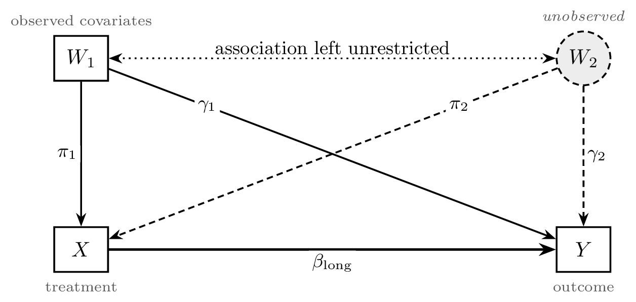
A diagram of the model. Boxes mark the observed variables W1, X and Y; a dashed circle marks the unobserved W2. Solid arrows pi-1 and gamma-1 run from W1 into X and Y, dashed arrows pi-2 and gamma-2 run from W2 into X and Y, and a heavy arrow labelled beta-long runs from X to Y. A dotted double-headed arrow between W1 and W2 is labelled association left unrestricted.

You want $\beta_{\text{long}}$ , the coefficient on the treatment $X$ in a regression that adjusts for everything relevant, observed or not. You can only run the medium regression, which adjusts for the observed covariates and returns $\beta_{\text{med}}$ . The two agree exactly when $\pi_2 = 0$ : no selection on unobservables, the dashed arrow into $X$ erased. Sensitivity analysis asks how far that can fail before your conclusion does.

Note what the baseline does not assume. It leaves $\gamma_2$ free – the unobservable may matter arbitrarily much for the outcome – and it leaves the $W_1$ – $W_2$ association free. That is why the observed controls being endogenous is not, on its own, fatal.

The observed covariates split in two. The ones you name in compare are the calibration covariates $W_1$ : the yardstick the unobservable is measured against. Everything else is a control covariate $W_0$ , adjusted for but never used as a yardstick – fixed effects and nuisance controls belong here. (Stata’s regsensitivity and this package’s argument names call $W_1$ the comparison set, which is where compare gets its name; the DMP paper calls it the calibration set. They are the same thing.)

library(regsensitivity)
library(ggplot2)
data(bfg2020)
bfg2020$statea <- factor(bfg2020$statea)

form <- avgrep2000to2016 ~ tye_tfe890_500kNI_100_l6 +
    log_area_2010 + lat + lon + temp_mean + rain_mean + elev_mean +
    d_coa + d_riv + d_lak + ave_gyi + statea
compare <- c("log_area_2010", "lat", "lon", "temp_mean", "rain_mean",
             "elev_mean", "d_coa", "d_riv", "d_lak", "ave_gyi")

So here the geographic and climate variables are $W_1$ and the state fixed effects statea are $W_0$ : the omitted variable’s importance is judged against geography and climate, never against state dummies. In general:

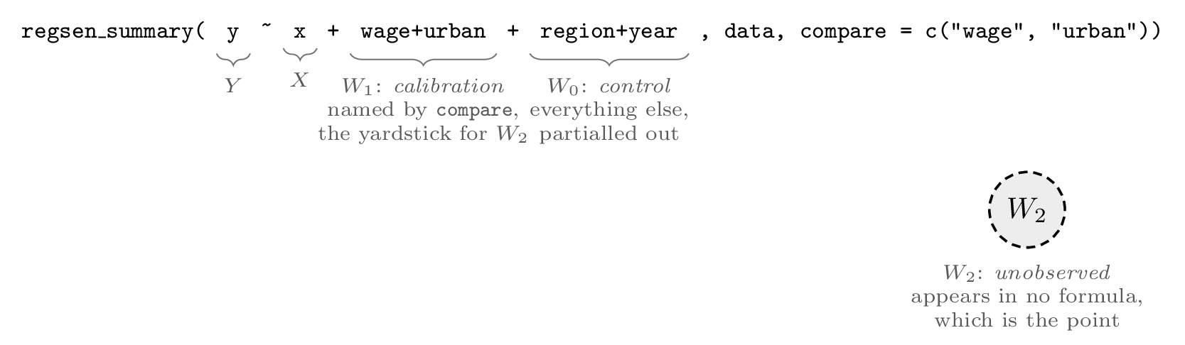
A regsen_summary call with braces under its parts: y is the outcome Y, x is the treatment X, the terms named by compare are the calibration covariates W1, and the remaining right-hand-side terms are the control covariates W0, which are partialled out. A dashed circle stands for the unobserved W2, which appears in no formula.

nocompare draws the same line from the other side, naming $W_0$ instead; give at most one of the two. If you give neither, every control enters $W_1$ .

The three sensitivity parameters

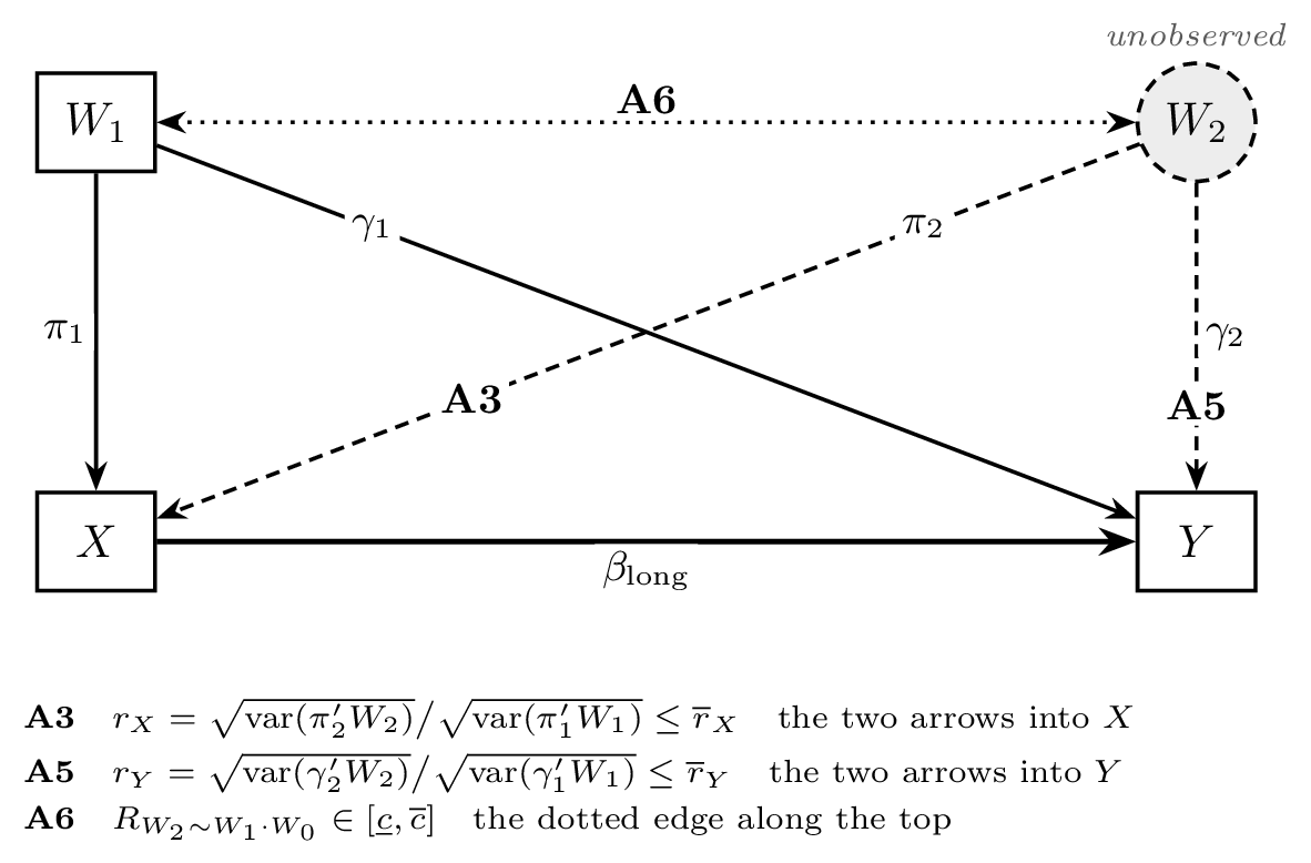
Rather than assume $\pi_2 = 0$ , DMP bound how large the unobservable’s role can be. Three parameters do the work, and each caps one feature of the picture above:

The same model diagram, with the dashed arrow from W2 into X tagged A3, the dashed arrow from W2 into Y tagged A5, and the dotted W1-W2 edge tagged A6. A key gives r-X as the ratio of the standard deviations of the two indices entering X, bounded by rxbar; r-Y likewise for Y, bounded by rybar; and the partial correlation of W2 with W1 given W0 lying in the interval from clow to cbar.

rxbar bounds $r_X$ : how much the unobservable moves the treatment, as a multiple of how much the calibration covariates do. rxbar = 1 says the unobservable is at most as important as $W_1$ taken together.
rybar bounds $r_Y$ : the same ratio for the outcome. Left at Inf by default, which assumes nothing about $\gamma_2$ .
cbar and clow bound how much of the unobservable the calibration covariates already explain. The default cbar = 1 imposes nothing, and is the case in which the controls may be arbitrarily endogenous.

Because $r_X$ and $r_Y$ are relative, their scale only means something against a reference; calibrate_rho() and calibrate_partial_r2() supply the point-identified reference values DMP propose.

The “short” regression coefficient (with no controls) and the “medium” regression coefficient (with state FE and the comparison controls) give a first sense of how much controls move the estimate:

short <- lm(avgrep2000to2016 ~ tye_tfe890_500kNI_100_l6, data = bfg2020)
med   <- lm(form, data = bfg2020)
coef(short)[2]
#> tye_tfe890_500kNI_100_l6 
#>                 1.707838
coef(med)["tye_tfe890_500kNI_100_l6"]
#> tye_tfe890_500kNI_100_l6 
#>                 2.054759

DMP (2026) bounds

regsen_bounds() is the workhorse. Out of the box it sweeps over a grid of rxbar from 0 to the threshold where the identified set first becomes $(-\infty,+\infty)$ , holding cbar fixed at the supplied value.

bnds <- regsen_bounds(form, bfg2020, compare = compare, cbar = 0.1)
print(bnds)
#> 
#> Regression Sensitivity Analysis ----- Bounds
#> ------------------------------------------------------------------------
#> Analysis:          DMP (2026)
#> Treatment:         tye_tfe890_500kNI_100_l6
#> Outcome:           avgrep2000to2016
#> N (obs):           2036
#> Hypothesis:        Beta > 0
#> Breakdown point:   1.1947
#> 
#> --- Summary statistics ----------------------------------
#>   Beta (short)                  1.9246
#>   Beta (medium)                 2.0548
#>   R2 (short)                    0.0328
#>   R2 (medium)                   0.1051
#>   Var(Y)                      101.7387
#>   Var(X)                        0.9014
#>   Var(X_Residual)               0.8823
#> 
#> --- Results ---------------------------------------------
#>   rxbar rybar   cbar     bmin   bmax
#>       0  +Inf    0.1   2.0548 2.0548
#>  0.4063  +Inf    0.1   1.4249 2.6846
#>  0.8126  +Inf    0.1  0.73082 3.3787
#>  1.2189  +Inf    0.1 -0.04935 4.1589
#>  1.6252  +Inf    0.1 -0.94897 5.0585
#>  2.0315  +Inf    0.1  -2.0229 6.1324
#>  2.4378  +Inf    0.1  -3.3697 7.4792
#>  2.8441  +Inf    0.1   -5.192 9.3015
#>  3.2504  +Inf    0.1  -8.0056 12.115
#>  3.6567  +Inf    0.1  -13.822 17.932
#>   4.063  +Inf    0.1     -Inf   +Inf

The bounds widen monotonically as rxbar (the strength of the unobservable’s effect on the treatment) grows. The breakdown point reported in the header is the rxbar value at which the hypothesis ( $\beta>0$ , in this case) first fails.

plot(bnds)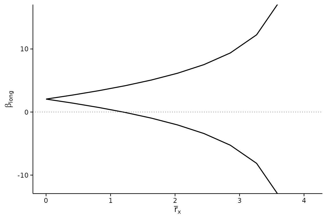

Sweeping over multiple cbar values lets you see how stronger correlations between the comparison controls and the unobservable affect the bounds:

multi <- regsen_bounds(form, bfg2020, compare = compare,
                        rxbar = seq(0, 2, length.out = 21),
                        cbar = c(0, 0.2, 0.4, 0.6, 0.8, 1.0))
plot(multi)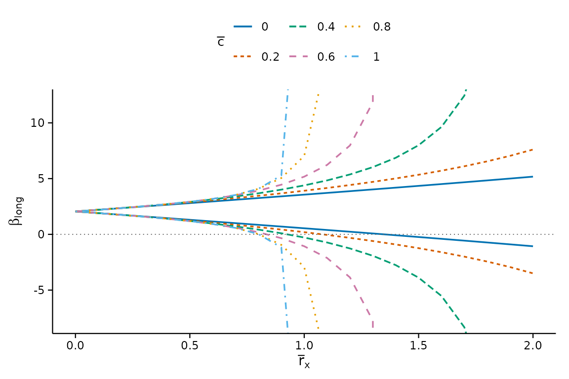

Constrained `rybar`

Setting rybar to a finite value adds a constraint on the unobservable’s effect on the outcome. When cbar > 0 this is a nonconvex problem and we solve it with a global optimizer (nloptr / DIRECT-L); when cbar = 0 it has a closed form. Both cases run through the same regsen_bounds() call:

fin <- regsen_bounds(form, bfg2020, compare = compare, rybar = 2)
print(fin)
#> 
#> Regression Sensitivity Analysis ----- Bounds
#> ------------------------------------------------------------------------
#> Analysis:          DMP (2026)
#> Treatment:         tye_tfe890_500kNI_100_l6
#> Outcome:           avgrep2000to2016
#> N (obs):           2036
#> Hypothesis:        Beta > 0
#> Breakdown point:   0.8035
#> 
#> --- Summary statistics ----------------------------------
#>   Beta (short)                  1.9246
#>   Beta (medium)                 2.0548
#>   R2 (short)                    0.0328
#>   R2 (medium)                   0.1051
#>   Var(Y)                      101.7387
#>   Var(X)                        0.9014
#>   Var(X_Residual)               0.8823
#> 
#> --- Results ---------------------------------------------
#>     rxbar  rybar   cbar     bmin   bmax
#>         0      2      1   2.0548 2.0548
#>  0.098939      2      1   1.9107 2.2007
#>   0.19788      2      1   1.7612 2.3539
#>   0.29682      2      1   1.5983 2.5185
#>   0.39576      2      1   1.4149 2.6989
#>   0.49469      2      1   1.2027 2.9069
#>   0.59363      2      1  0.94779 3.1617
#>   0.69257      2      1  0.60803 3.5015
#>   0.79151      2      1 0.086812 4.0227
#>   0.89045      2      1 -0.99272 5.1022
#>   0.98939      2      1     -Inf   +Inf

You can also express rybar as a function of rxbar, e.g. rybar = rxbar:

expr <- regsen_bounds(form, bfg2020, compare = compare,
                       rybar_expr = function(rx) rx,
                       rxbar = seq(0, 1, 0.1))
expr$results
#>    rxbar rybar cbar     bmin     bmax
#> 1    0.0   0.0    1 2.054759 2.054759
#> 2    0.1   0.1    1 2.050500 2.059033
#> 3    0.2   0.2    1 2.037541 2.072210
#> 4    0.3   0.3    1 2.015278 2.095477
#> 5    0.4   0.4    1 1.982458 2.131293
#> 6    0.5   0.5    1 1.936611 2.184491
#> 7    0.6   0.6    1 1.872585 2.265157
#> 8    0.7   0.7    1 1.778058 2.397467
#> 9    0.8   0.8    1 1.615327 2.656118
#> 10   0.9   0.9    1 1.189271 3.438830
#> 11   1.0   1.0    1     -Inf      Inf

DMP breakdown

regsen_breakdown() reports the breakdown point as a function of one of the sensitivity parameters, holding the others fixed:

bd <- regsen_breakdown(form, bfg2020, compare = compare,
                        cbar = seq(0, 1, 0.05))
plot(bd)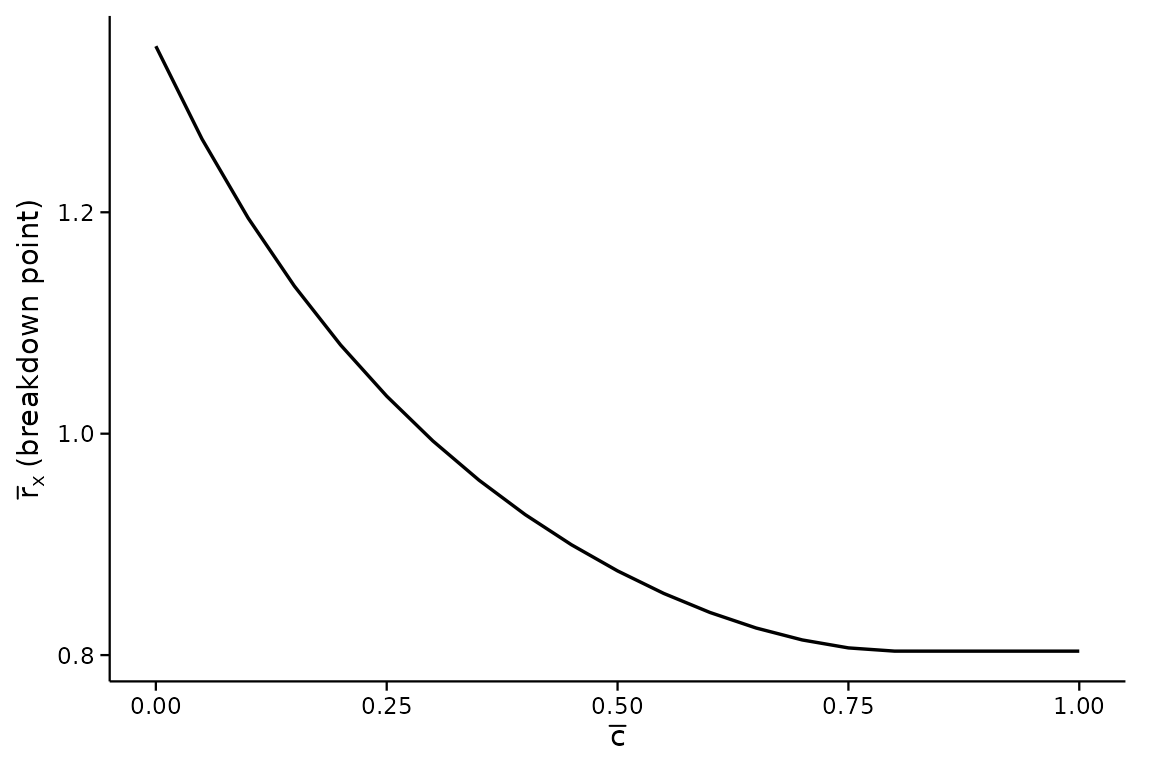

You can also sweep across hypothesis values:

hyp <- regsen_breakdown(form, bfg2020, compare = compare,
                         beta = bnd_lb(seq(-1, 1, 0.2)))
print(hyp)
#> 
#> Regression Sensitivity Analysis ----- Breakdown Frontier
#> ------------------------------------------------------------------------
#> Analysis:          DMP (2026)
#> Treatment:         tye_tfe890_500kNI_100_l6
#> Outcome:           avgrep2000to2016
#> N (obs):           2036
#> Hypothesis:        Beta > Beta(Hypothesis)
#> 
#> --- Summary statistics ----------------------------------
#>   Beta (short)                  1.9246
#>   Beta (medium)                 2.0548
#>   R2 (short)                    0.0328
#>   R2 (medium)                   0.1051
#>   Var(Y)                      101.7387
#>   Var(X)                        0.9014
#>   Var(X_Residual)               0.8823
#> 
#> --- Results ---------------------------------------------
#>   index breakdown
#>      -1   0.89085
#>    -0.8   0.87887
#>    -0.6   0.86473
#>    -0.4   0.84792
#>    -0.2    0.8278
#>       0   0.80356
#>     0.2   0.77418
#>     0.4   0.73835
#>     0.6   0.69452
#>     0.8   0.64083
#>       1   0.57525

The frontier in the other direction

direction = "rybar" reports the breakdown point in rybar at each rxbar instead: how much the unobservable may matter for the outcome before the conclusion fails, given how much it may matter for the treatment. This is the frontier of DMP Theorem 4, and the two directions trace the same curve in the $(\bar r_X, \bar r_Y)$ plane.

fr <- regsen_breakdown(form, bfg2020, compare = compare, cbar = 1,
                        direction = "rybar",
                        rxbar = c(0.5, 1, 2, 4))
fr$results
#>   index breakdown
#> 1   0.5       Inf
#> 2   1.0 0.8632973
#> 3   2.0 0.5901671
#> 4   4.0 0.5901671

An Inf says the conclusion survives every rybar at that rxbar; the mirror image, an Inf from the default direction, says it survives every rxbar at that rybar.

Asserting endogenous controls

cbar caps how much of the unobservable the comparison controls can explain. clow is the other end of DMP Assumption A6: setting it above zero asserts that the controls are at least that endogenous, which narrows the identified set rather than widening it.

vapply(c(0, 0.9, 0.99), function(cl) {
    regsen_breakdown(form, bfg2020, compare = compare,
                      cbar = 1, clow = cl)$results$breakdown
}, numeric(1))
#> [1] 0.8035643 0.8177462 0.9136661

Oster (2019) bounds

Switching to the Oster analysis with analysis = "oster":

o <- regsen_bounds(form, bfg2020, compare = compare,
                    analysis = "oster")
print(o)
#> 
#> Regression Sensitivity Analysis ----- Bounds
#> ------------------------------------------------------------------------
#> Analysis:          Oster (2019)
#> Treatment:         tye_tfe890_500kNI_100_l6
#> Outcome:           avgrep2000to2016
#> N (obs):           2036
#> Hypothesis:        Beta > 0
#> Breakdown point:   1.7039
#> 
#> --- Summary statistics ----------------------------------
#>   Beta (short)                  1.9246
#>   Beta (medium)                 2.0548
#>   R2 (short)                    0.0328
#>   R2 (medium)                   0.1051
#>   Var(Y)                      101.7387
#>   Var(X)                        0.9014
#>   Var(X_Residual)               0.8823
#> 
#> --- Results ---------------------------------------------
#>   delta r2long   beta1  beta2 beta3
#>      -1      1 0.69842             
#>    -0.8      1 0.93048             
#>    -0.6      1  1.1801             
#>    -0.4      1   1.449             
#>    -0.2      1  1.7396             
#>       0      1  2.0548             
#>     0.2      1  2.3981             
#>     0.4      1  2.7747             
#>     0.6      1  3.1917             
#>     0.8      1  3.6595             
#>       1      1 -46.171 4.1944

Plotting the equality identified set (rotated so that delta is on the x-axis and beta on the y-axis):

o2 <- regsen_bounds(form, bfg2020, compare = compare,
                     analysis = "oster",
                     delta = seq(-3, 3, 0.05))
plot(o2, ylim = c(-5, 8))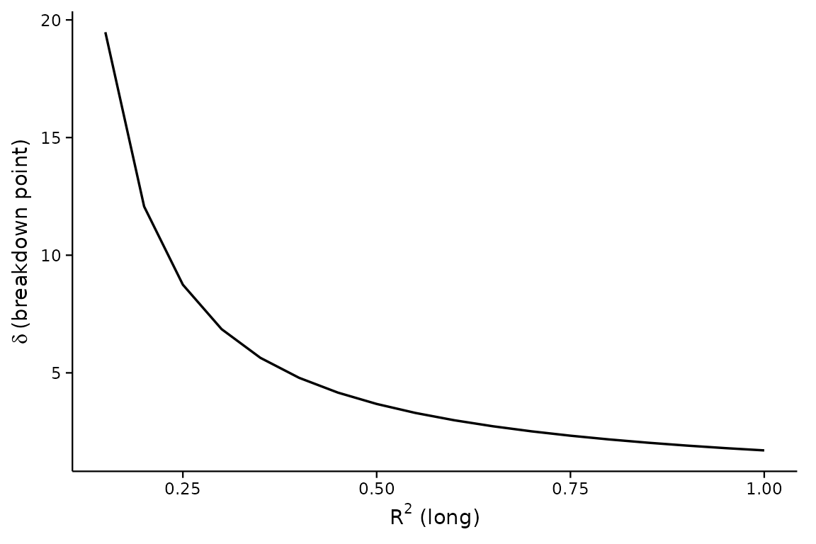

Oster, |delta| <= d (bound)

ob <- regsen_bounds(form, bfg2020, compare = compare,
                     analysis = "oster",
                     delta = seq(0, 0.999, 0.001),
                     delta_type = "bound")
plot(ob, ylim = c(-50, 50))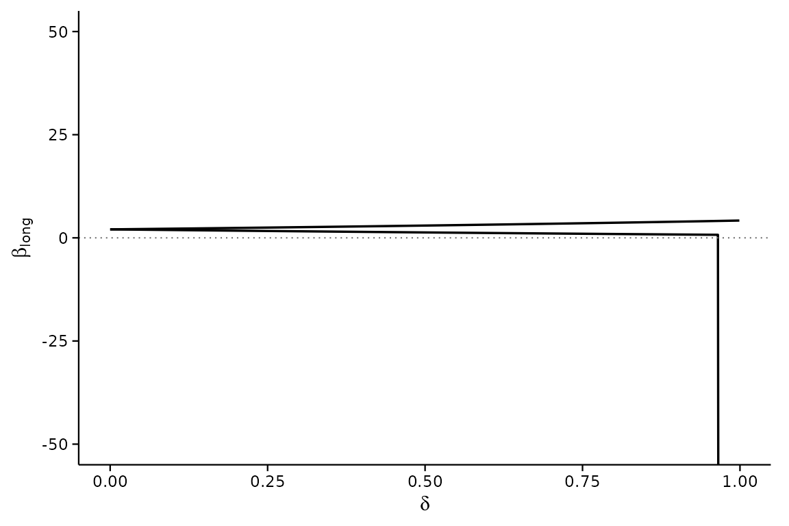

Oster breakdown

obd_eq <- regsen_breakdown(form, bfg2020, compare = compare,
                            analysis = "oster",
                            r2long = seq(0.15, 1, 0.05),
                            beta = bnd_eq(0))
plot(obd_eq)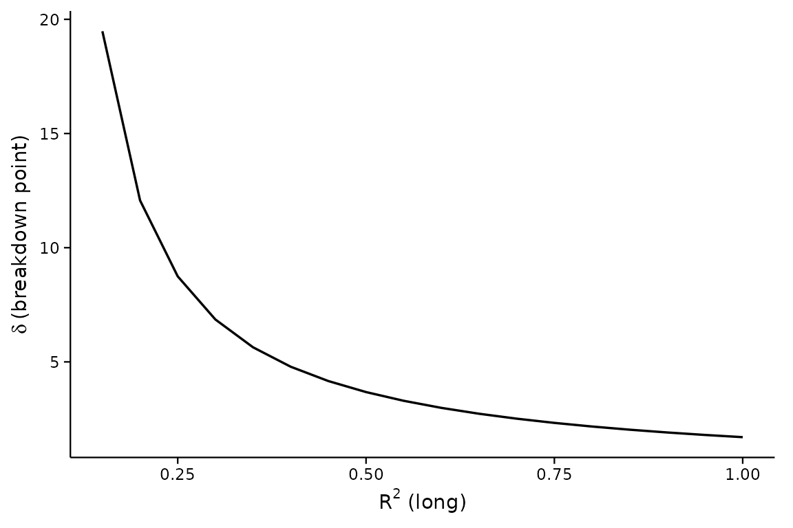


obd_sign <- regsen_breakdown(form, bfg2020, compare = compare,
                              analysis = "oster",
                              r2long = seq(0.15, 1, 0.05))
plot(obd_sign)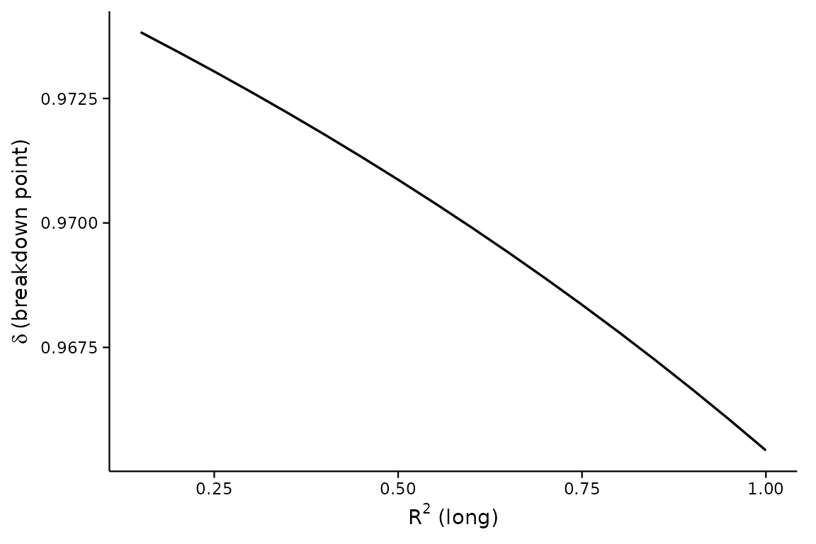

Using several cores

Everything above runs on one core by default. The finite-rybar sweeps and the breakdown frontiers are the slow parts – each grid point or frontier value is a global optimization – and they are independent, so they can be spread across cores. Set the session default once:

regsen_cores(2)        # a number of cores

regsen_cores("auto") takes every core but two, leaving the session and whatever else the machine is doing responsive. Whatever you set, at most two are used while R CMD check --as-cran runs, which forbids more.

or pass ncores to a single call of regsen_bounds(), regsen_breakdown(), regsen_multi() or regsen_boot(). Results are identical whatever the number of cores; the bootstrap seeds each replicate itself, and nothing else draws random numbers.

Summary call

When you don’t know where to start, regsen_summary() runs the default DMP bounds analysis plus an Oster breakdown sweep at a few standard r2long values, matching the behaviour of Stata’s regsensitivity with no subcommand.

s <- regsen_summary(form, bfg2020, compare = compare)
print(s)
#> 
#> === DMP (2026) bounds ===
#> 
#> Regression Sensitivity Analysis ----- Bounds
#> ------------------------------------------------------------------------
#> Analysis:          DMP (2026)
#> Treatment:         tye_tfe890_500kNI_100_l6
#> Outcome:           avgrep2000to2016
#> N (obs):           2036
#> Hypothesis:        Beta > 0
#> Breakdown point:   0.8036
#> 
#> --- Summary statistics ----------------------------------
#>   Beta (short)                  1.9246
#>   Beta (medium)                 2.0548
#>   R2 (short)                    0.0328
#>   R2 (medium)                   0.1051
#>   Var(Y)                      101.7387
#>   Var(X)                        0.9014
#>   Var(X_Residual)               0.8823
#> 
#> --- Results ---------------------------------------------
#>     rxbar rybar   cbar     bmin   bmax
#>         0  +Inf      1   2.0548 2.0548
#>  0.098939  +Inf      1   1.9064 2.2031
#>   0.19788  +Inf      1   1.7535  2.356
#>   0.29682  +Inf      1   1.5906 2.5189
#>   0.39576  +Inf      1   1.4106 2.6989
#>   0.49469  +Inf      1   1.2026 2.9069
#>   0.59363  +Inf      1  0.94779 3.1617
#>   0.69257  +Inf      1  0.60803 3.5015
#>   0.79151  +Inf      1 0.086812 4.0227
#>   0.89045  +Inf      1 -0.99272 5.1022
#>   0.98939  +Inf      1     -Inf   +Inf
#> 
#> === Oster (2019) breakdown ===
#> 
#> Regression Sensitivity Analysis ----- Breakdown Frontier
#> ------------------------------------------------------------------------
#> Analysis:          Oster (2019)
#> Treatment:         tye_tfe890_500kNI_100_l6
#> Outcome:           avgrep2000to2016
#> N (obs):           2036
#> Hypothesis:        Beta > 0
#> 
#> --- Summary statistics ----------------------------------
#>   Beta (short)                  1.9246
#>   Beta (medium)                 2.0548
#>   R2 (short)                    0.0328
#>   R2 (medium)                   0.1051
#>   Var(Y)                      101.7387
#>   Var(X)                        0.9014
#>   Var(X_Residual)               0.8823
#> 
#> --- Results ---------------------------------------------
#>    index breakdown
#>  0.13667   0.97393
#>  0.23667   0.97315
#>  0.33667   0.97232
#>  0.43667   0.97145
#>  0.53667   0.97052
#>  0.63667   0.96954
#>  0.73667    0.9685
#>  0.83667   0.96739
#>  0.93667   0.96622
#>        1   0.96543

References

Diegert, P., Masten, M., and Poirier, A. (2026). Assessing Omitted Variable Bias when the Controls are Endogenous. arXiv:2206.02303.
Oster, E. (2019). Unobservable Selection and Coefficient Stability: Theory and Evidence. JBES 37(2), 187–204.
Masten, M., and Poirier, A. (2026). The Effect of Omitted Variables on the Sign of Regression Coefficients. AER 116(7), 2685–2710.
Bazzi, S., Fiszbein, M., and Gebresilasse, M. (2020). Frontier Culture: The Roots and Persistence of “Rugged Individualism” in the United States. Econometrica 88(6), 2329–2368.