Stylized examples from Masten and Poirier (2026)

This vignette illustrates, on a stylized constructed example, the figures of Masten and Poirier (2026), The Effect of Omitted Variables on the Sign of Regression Coefficients. The paper’s Figures 1, 2, and S1 are built on its empirical application to Satyanath, Voigtländer and Voth (2017), whose microdata is distributed separately (Harvard Dataverse, doi:10.7910/DVN/EE6I7N) and is not bundled here; the paper itself does not print the moments needed to regenerate those curves. Its survey tables aggregate across many published studies. So this vignette exercises the machinery in regsensitivity end-to-end on a data-generating process we control, and the structural features of the published figures – at most three branches, the vertical asymptote at $\delta = 1$ – are what should carry over. The numerical values should not be compared.

A stylized data-generating process

We construct a small example where the medium-regression coefficient is positive but Oster’s identified set $\mathcal{B}_I(\delta, R_{long})$ crosses zero at moderate $\delta$.

library(regsensitivity)
library(ggplot2)

set.seed(2208)
n <- 5000
w1 <- rnorm(n)
w2 <- rnorm(n)
x  <- 0.3 * w1 + 0.5 * w2 + rnorm(n)
y  <- 0.8 * x + 0.4 * w1 + 0.6 * w2 + rnorm(n)
dat <- data.frame(y = y, x = x, w1 = w1)   # w2 is unobserved!

form <- y ~ x + w1

The “true” long-regression coefficient is 0.8; the medium regression sees an upward-biased estimate because w2 is correlated with x.

coef(lm(y ~ x + w1, data = dat))["x"]
#>        x 
#> 1.025787

Figure 1: Oster’s identified set $\mathcal{B}_I(\delta, R_{long})$

res <- regsen_bounds(form, dat,
                      analysis = "oster",
                      delta = seq(-2, 2, 0.02),
                      r2long = 1)
plot(res, ylim = c(-2, 4),
     title = "Figure 1 (stylized): Oster identified set vs delta")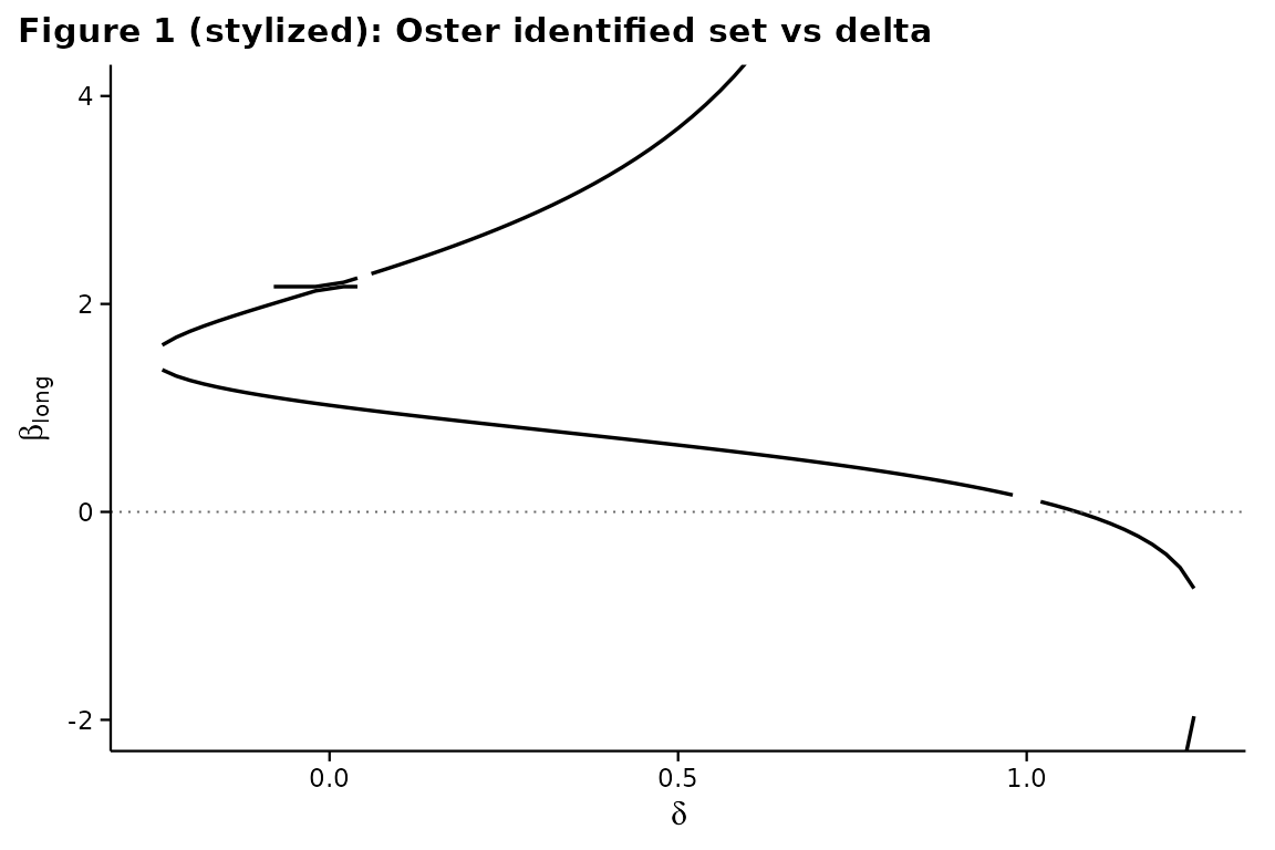

The branches of the cubic in $\beta$ that solve Oster’s equation give the identified set. As $\delta \to 1$ from either side, the branches diverge (asymptotes are roots of the cubic’s denominator).

Figure 2: cumulative identified set $\delta \le \bar d$

res2 <- regsen_bounds(form, dat,
                       analysis = "oster",
                       delta = seq(0, 0.99, 0.005),
                       delta_type = "bound",
                       r2long = 1)
plot(res2, ylim = c(-5, 5),
     title = "Figure 2 (stylized): cumulative identified set")

Table 1: breakdown points

Quantity	Value
oster_breakdown_eq, $\beta = 0$, $R_{long}=1$	1.0725
oster_breakdown_bound, $\beta > 0$, $R_{long}=1$	1
DMP $\bar r_X^{bp}$ at $\bar c = 1$	0.9424

Effect of a maxovb constraint

Masten-Poirier (2026) extend Oster by adding a maximum omitted variable bias constraint. We illustrate by varying maxovb:

ovbs <- seq(0.05, 0.5, 0.05)
out <- lapply(ovbs, function(M) {
    r <- regsen_breakdown(form, dat,
                           analysis = "oster",
                           r2long = 1, maxovb = M)
    data.frame(maxovb = M, breakdown = r$results$breakdown[1])
})
out <- do.call(rbind, out)
ggplot(out, aes(maxovb, breakdown)) +
    geom_line() + geom_point() +
    labs(x = "maxovb", y = "Delta (breakdown)",
         title = "Oster breakdown vs max OVB")

A tighter cap on the OVB magnitude lifts the breakdown delta.

Meta-analysis tables (paper Tables 3-4)

The paper’s Tables 3 and 4 aggregate breakdown-point statistics across many published studies. (Table 2 belongs to the Satyanath et al. application, not the survey.) The package contains the primitives needed to reproduce those tables (regsen_breakdown(... maxovb = ...)); plug your own meta-analysis data in and call:

results <- lapply(study_list, function(study) {
    out <- regsen_breakdown(study$formula, study$data,
                             analysis = "oster",
                             r2long = 1, maxovb = study$maxovb,
                             beta = bnd_eq(0))
    out$results$breakdown[1]
})