Financial Fraud Detection

Financial Fraud Detection#

Financial fraud is a pervasive and evolving threat that undermines the integrity of financial systems, erodes trust among stakeholders, and results in substantial economic losses worldwide. As financial transactions become increasingly digitized and complex, the methods employed by fraudsters continue to advance, necessitating sophisticated detection and prevention mechanisms. This chapter offers an in-depth exploration of financial fraud detection, encompassing a comprehensive classification of fraud types, detailed methodologies utilized in the literature, evaluation metrics, common challenges, innovative approaches, and a thorough Python-based data pipeline demonstration using synthetic data.

. References

1. Introduction#

Financial fraud encompasses a broad spectrum of illicit activities aimed at deceiving individuals, organizations, or institutions for financial gain. The proliferation of digital technologies, online banking, and e-commerce has significantly expanded the avenues through which fraudsters operate, making detection and prevention increasingly challenging. Effective fraud detection systems are critical for mitigating financial losses, maintaining stakeholder trust, and ensuring compliance with regulatory standards.

The dynamic and adaptive nature of financial fraud necessitates the continuous evolution of detection methodologies. Traditional rule-based systems are often insufficient in capturing the sophisticated and subtle patterns indicative of fraudulent behavior. Consequently, the integration of advanced machine learning (ML) and artificial intelligence (AI) techniques has become indispensable in developing robust and scalable fraud detection frameworks.

This chapter delves into the multifaceted domain of financial fraud detection, providing a detailed classification of fraud types, exploring a wide array of detection methodologies, discussing essential evaluation metrics, addressing common challenges, showcasing innovative approaches, and presenting a comprehensive Python-based data pipeline using synthetic data for practical understanding.

2. Types of Financial Fraud#

Financial fraud can be classified based on various dimensions, including the nature of the fraud, the target, the perpetrator, and the method of execution. A nuanced understanding of these categories is essential for developing targeted and effective detection strategies. Below is a comprehensive classification tailored to encompass a broad spectrum of fraudulent activities.

2.1. Transaction Fraud#

Transaction fraud involves deceitful activities aimed at manipulating financial transactions to illegitimately gain funds. This category includes:

Credit Card Fraud: Unauthorized use of credit card information to make purchases or withdraw cash. Subtypes include:
- Card Not Present (CNP) Fraud: Occurs in online or phone transactions where the physical card is not required.
- Card Present Fraud: Involves physical misuse of the card, such as cloning or skimming.
Wire Transfer Fraud: Unauthorized initiation of electronic funds transfers, often facilitated through phishing or malware attacks.
Account Takeover (ATO): Gaining unauthorized access to a legitimate user’s account to perform fraudulent transactions.

2.3. Internal Fraud#

Internal fraud refers to fraudulent activities perpetrated by individuals within an organization. Types include:

Embezzlement: Misappropriation of funds entrusted to an employee’s care.
Payroll Fraud: Manipulating payroll systems to receive unauthorized payments, such as ghost employees or inflated salaries.
Expense Reimbursement Fraud: Submitting false expense claims for personal gain.

2.4. Cyber-Fraud#

Cyber-fraud encompasses fraudulent activities executed through digital platforms and technologies. It includes:

Phishing: Deceptive attempts to obtain sensitive information by masquerading as a trustworthy entity.
Ransomware Attacks: Encrypting an organization’s data and demanding payment for its release.
Business Email Compromise (BEC): Targeting employees with access to company finances through deceptive emails to initiate unauthorized transactions.

2.5. Advanced and Emerging Fraud Types#

Beyond the primary categories, several advanced and emerging types of financial fraud have gained prominence:

Fraud Type	Description
Securities Fraud	Manipulation of stock prices, insider trading, or dissemination of false information to deceive investors.
Mortgage Fraud	Misrepresentation in mortgage applications, property valuations, or foreclosure processes.
Insurance Fraud	Filing false or exaggerated insurance claims to receive unwarranted payouts, including health, auto, and property.
Money Laundering	Concealing the origins of illicitly obtained money, typically by transferring through complex transactions.
Cryptocurrency Fraud	Scams involving digital currencies, such as fake ICOs (Initial Coin Offerings), exchange hacks, or Ponzi schemes.
Tax Fraud	Deliberate falsification of information on tax returns to reduce tax liability or avoid taxes.
Vendor Fraud	Manipulating vendor relationships to receive unauthorized payments or services.
Ponzi and Pyramid Schemes	Investment scams promising high returns with little risk, relying on new investors to pay returns to earlier ones.

Understanding these diverse types of financial fraud is crucial for developing comprehensive detection and prevention strategies tailored to each fraud’s unique characteristics.

3. Methods Used in Literature for Fraud Detection#

The landscape of financial fraud detection has been significantly shaped by advancements in machine learning, artificial intelligence, and statistical methodologies. Researchers and practitioners have developed and employed a myriad of techniques to identify and prevent fraudulent activities. This section categorizes these methods into supervised, unsupervised, semi-supervised, reinforcement learning, and hybrid approaches, providing a detailed overview of each.

3.1. Supervised Learning Methods#

Supervised learning involves training models on labeled datasets where the outcome (fraudulent or legitimate) is known. These methods are widely used due to their effectiveness in classification tasks.

Method	Description	Advantages	Disadvantages
Support Vector Machine (SVM)	Constructs hyperplanes in high-dimensional space to separate classes. Utilizes kernel functions to handle non-linear data.	Effective in high-dimensional spaces; Robust against overfitting with clear margin separation.	Computationally intensive with large datasets; Less effective with overlapping classes.
Decision Trees	Models decisions and their possible consequences as a tree-like structure. Splits data based on feature values to predict the target variable.	Easy to interpret and visualize; Handles both numerical and categorical data.	Prone to overfitting; Can become complex with large datasets.
Logistic Regression	Estimates the probability of a binary outcome using the logistic function based on input features.	Simple and interpretable; Efficient for linearly separable data.	Limited to linear decision boundaries; Less effective with complex relationships.
Naive Bayes	Probabilistic classifiers based on Bayes’ theorem, assuming feature independence.	Fast and efficient; Performs well with high-dimensional data.	Independence assumption may not hold; Less accurate when features are correlated.
Random Forest	An ensemble method that builds multiple decision trees and aggregates their predictions.	High accuracy and robustness; Handles large datasets with high dimensionality.	Less interpretable than single decision trees; Can be computationally intensive.
Gradient Boosting Machines (GBM)	Builds trees sequentially, where each tree attempts to correct the errors of the previous one. Examples include XGBoost, LightGBM, and CatBoost.	High predictive performance; Handles various data types and complexities.	Prone to overfitting if not properly tuned; Computationally intensive.
K-Nearest Neighbors (K-NN)	Classifies instances based on the majority class among the K nearest neighbors in the feature space.	Simple and easy to implement; No training phase required.	Computationally intensive during prediction; Sensitive to the choice of K and distance metric.
Neural Networks (ANN)	Composed of interconnected layers of neurons that can model complex, non-linear relationships in data.	Capable of capturing complex patterns; Highly flexible and adaptable.	Requires large amounts of data; Computationally intensive and less interpretable.

3.2. Unsupervised Learning Methods#

Unsupervised learning deals with unlabeled data, aiming to identify inherent structures or patterns. These methods are particularly useful for anomaly detection in fraud.

Method	Description	Advantages	Disadvantages
K-Means Clustering	Partitions data into K clusters based on distance metrics, grouping similar data points together.	Simple and scalable; Effective with well-separated clusters.	Requires specification of K; Sensitive to initial centroid placement and outliers.
DBSCAN (Density-Based Spatial Clustering of Applications with Noise)	Identifies clusters based on density, effectively detecting outliers and arbitrary-shaped clusters.	Does not require specifying the number of clusters; Effective at identifying outliers.	Struggles with varying density; Computationally intensive with large datasets.
Isolation Forest	An ensemble method that isolates anomalies by randomly partitioning the data.	Effective for high-dimensional data; Handles large datasets efficiently.	May struggle with data containing multiple types of anomalies; Parameter tuning required.
One-Class SVM	Learns a decision boundary around the majority class to identify outliers.	Effective for novelty detection; Can handle non-linear boundaries with kernel functions.	Sensitive to parameter selection; Less effective with high-dimensional data.
Principal Component Analysis (PCA)	Reduces dimensionality by transforming data into principal components, highlighting variance and potential anomalies.	Effective for dimensionality reduction; Enhances computational efficiency.	May not capture complex, non-linear relationships; Interpretation of components can be challenging.

3.3. Semi-Supervised and Reinforcement Learning Methods#

These methods leverage both labeled and unlabeled data or learn optimal actions through interaction with an environment.

Method	Description	Advantages	Disadvantages
Semi-Supervised Learning	Combines a small amount of labeled data with a large amount of unlabeled data during training.	Utilizes abundant unlabeled data; Can improve learning accuracy with limited labeled data.	Complexity in model training; Requires appropriate balance between labeled and unlabeled data.
Reinforcement Learning (RL)	Learns optimal actions through trial and error interactions with the environment, receiving rewards or penalties based on actions taken.	Capable of learning sequential decision-making processes; Adaptable to dynamic environments.	Requires significant computational resources; Challenges in defining appropriate reward structures.

3.4. Hybrid and Ensemble Methods#

Hybrid and ensemble methods combine multiple algorithms or techniques to enhance predictive performance and robustness.

Method	Description	Advantages	Disadvantages
Ensemble Learning	Combines the predictions of multiple models to improve overall performance. Techniques include Bagging, Boosting, and Stacking.	Enhances predictive accuracy; Reduces overfitting; Increases robustness against individual model weaknesses.	Increased computational complexity; Reduced interpretability.
Hybrid Models	Integrates different types of models or combines multiple methodologies (e.g., combining supervised and unsupervised learning) to leverage their complementary strengths.	Can capture a broader range of patterns and anomalies; Flexible in adapting to complex data structures.	Complexity in model integration; Potential challenges in parameter tuning and optimization.
Voting Classifiers	Aggregates predictions from multiple classifiers using majority voting or weighted voting schemes.	Simple to implement; Can improve overall classification performance.	Requires diverse base classifiers for maximum effectiveness; May still be biased towards majority classes.

3.5. Emerging and Advanced Methods#

Recent advancements have introduced novel methodologies to enhance fraud detection capabilities further.

Method	Description	Advantages	Disadvantages
Graph Neural Networks (GNNs)	Models relational data as graphs, capturing intricate relationships between entities (e.g., transactions, accounts) to detect fraud patterns.	Effective at modeling complex relational data; Can uncover hidden patterns and connections.	Computationally intensive; Requires appropriate graph structure and representation.
Deep Learning Architectures	Advanced neural network structures, including Convolutional Neural Networks (CNNs) and Long Short-Term Memory (LSTM) networks, capable of capturing spatial and temporal dependencies in data.	High capacity for learning complex, non-linear relationships; Suitable for large-scale data.	Requires large datasets and substantial computational resources; Less interpretable.
Quantum Machine Learning	Integrates quantum computing principles with machine learning algorithms to enhance processing capabilities and handle large, complex datasets more efficiently.	Potential for significant speedups in processing; Capable of handling high-dimensional data more effectively.	Currently in nascent stages; Requires specialized hardware and expertise.
Autoencoders for Anomaly Detection	Unsupervised neural networks that learn compressed representations of data, useful for reconstructing normal transactions and identifying anomalies based on reconstruction errors.	Effective for dimensionality reduction and anomaly detection; Can capture non-linear relationships.	Requires careful tuning; May not perform well with highly imbalanced data without modifications.
Transfer Learning	Utilizes knowledge gained from one domain or task to improve learning in another related domain or task, enhancing model performance with limited data.	Reduces training time; Can improve performance with limited labeled data.	May require substantial computational resources; Effectiveness depends on the similarity between domains.

4. Evaluation Metrics Used in Fraud Detection#

Evaluating the performance of fraud detection models is critical to ensure their effectiveness and reliability. Given the typically imbalanced nature of fraud datasets, where fraudulent instances are significantly rarer than legitimate ones, selecting appropriate evaluation metrics is essential.

4.1. Accuracy#

Accuracy measures the proportion of correctly classified instances out of the total instances.

\[ \text{Accuracy} = \frac{TP + TN}{TP + TN + FP + FN} \]

Pros: Simple to understand and compute.
Cons: Can be misleading in imbalanced datasets, as a model may achieve high accuracy by predominantly predicting the majority class.

4.2. Precision#

Precision (also known as Positive Predictive Value) measures the proportion of true positive predictions among all positive predictions made by the model.

\[ \text{Precision} = \frac{TP}{TP + FP} \]

Pros: Indicates the model’s ability to avoid false positives.
Cons: Does not account for false negatives, potentially overlooking undetected fraud cases.

4.3. Recall/Sensitivity/True Positive Rate (TPR)#

Recall (also known as Sensitivity or True Positive Rate) measures the proportion of actual positive instances correctly identified by the model.

\[ \text{Recall} = \frac{TP}{TP + FN} \]

Pros: Reflects the model’s ability to detect actual fraud cases.
Cons: Does not account for false positives, which can lead to unnecessary investigations.

4.4. F-measure (F1 Score)#

F1 Score is the harmonic mean of precision and recall, providing a balance between the two.

\[ F1 = 2 \times \frac{\text{Precision} \times \text{Recall}}{\text{Precision} + \text{Recall}} \]

Pros: Balances precision and recall, especially useful when seeking a trade-off between the two.
Cons: Does not consider true negatives, which might be relevant in certain contexts.

4.5. Specificity (True Negative Rate, TNR)#

Specificity measures the proportion of actual negative instances correctly identified by the model.

\[ \text{Specificity} = \frac{TN}{TN + FP} \]

Pros: Indicates the model’s ability to correctly identify legitimate transactions.
Cons: Does not account for false negatives, potentially missing fraudulent activities.

4.6. Area Under the Receiver Operating Characteristic Curve (AUC-ROC)#

AUC-ROC evaluates the model’s ability to distinguish between classes across various threshold settings.

Pros: Provides a single metric summarizing the model’s discriminative ability; Robust to class imbalance.
Cons: Does not provide information about the optimal threshold; Can be less informative for highly imbalanced datasets.

4.7. Matthews Correlation Coefficient (MCC)#

MCC is a metric that considers true and false positives and negatives, providing a balanced measure even with class imbalance.

\[ \text{MCC} = \frac{TP \times TN - FP \times FN}{\sqrt{(TP + FP)(TP + FN)(TN + FP)(TN + FN)}} \]

Pros: Produces a value between -1 and +1, where +1 indicates perfect prediction, 0 no better than random, and -1 indicates total disagreement between prediction and observation.
Cons: More complex to interpret compared to simpler metrics.

4.8. Cost-Based Metrics#

In real-world applications, the cost of different types of errors (false positives vs. false negatives) varies. Cost-based metrics incorporate the financial implications of these errors into the evaluation.

\[ \text{Cost} = FP \times \text{Cost}_{FP} + FN \times \text{Cost}_{FN} \]

Pros: Aligns model evaluation with business objectives and financial implications.
Cons: Requires accurate estimation of the costs associated with different types of errors.

4.9. Precision-Recall Curve#

A precision-recall curve plots precision against recall for different threshold values, providing insights into the trade-offs between the two metrics.

Pros: More informative than ROC curves for imbalanced datasets.
Cons: Does not account for true negatives.

5. Common Challenges in Financial Fraud Detection#

Detecting financial fraud is fraught with challenges that stem from the nature of fraudulent activities, data limitations, and evolving tactics of fraudsters. Understanding these challenges is crucial for developing effective detection systems.

5.1. Imbalanced Datasets#

Issue: In financial datasets, fraudulent instances are typically much rarer than legitimate ones, leading to class imbalance. This imbalance can bias models towards predicting the majority class, reducing their effectiveness in detecting fraud.

Solutions:

Oversampling Techniques: Methods like SMOTE (Synthetic Minority Over-sampling Technique) generate synthetic samples for the minority class to balance the dataset.
Undersampling Techniques: Reducing the number of majority class samples to balance the class distribution.
Cost-Sensitive Learning: Assigning higher misclassification costs to the minority class to penalize false negatives more severely.
Anomaly Detection Approaches: Focusing on identifying outliers rather than balancing classes.

5.2. Data/Concept Drift#

Issue: Fraud patterns evolve over time as fraudsters adapt their tactics, leading to changes in data distributions. This phenomenon, known as concept drift, can degrade model performance if not addressed.

Solutions:

Continuous Model Updating: Regularly retraining models with new data to capture evolving patterns.
Adaptive Learning Algorithms: Models that can dynamically adjust to new patterns without complete retraining.
Monitoring and Drift Detection: Implementing systems to detect when drift occurs and trigger model updates or alerts.

5.3. Feature Selection and Engineering#

Issue: Identifying relevant features that effectively capture fraud patterns is critical. Irrelevant or redundant features can degrade model performance and increase computational complexity.

Solutions:

Statistical Methods: Techniques like correlation analysis and mutual information to identify relevant features.
Dimensionality Reduction: Methods like PCA (Principal Component Analysis) to reduce feature space while retaining essential information.
Domain Expertise: Leveraging knowledge from financial experts to select and engineer meaningful features.

5.4. Scalability and Real-Time Detection#

Issue: Handling large volumes of transactions in real-time requires efficient algorithms and robust infrastructure, posing computational and scalability challenges.

Solutions:

Distributed Computing: Utilizing frameworks like Hadoop or Spark to process large datasets in parallel.
Efficient Algorithms: Employing lightweight models optimized for speed and low latency.
Incremental Learning: Updating models incrementally without retraining from scratch, enabling real-time adaptability.

5.5. Interpretability and Explainability#

Issue: Stakeholders often require explanations for fraud detection decisions to ensure trust, compliance, and actionable insights. Black-box models may hinder this transparency.

Solutions:

Model-Agnostic Methods: Techniques like SHAP (SHapley Additive exPlanations) and LIME (Local Interpretable Model-agnostic Explanations) provide explanations for complex models.
Interpretable Models: Choosing inherently interpretable models like decision trees or logistic regression when possible.
Hybrid Approaches: Combining complex models with simpler, interpretable models to balance performance and explainability.

5.6. Data Privacy and Security#

Issue: Handling sensitive financial data requires stringent adherence to data privacy laws and security standards. Ensuring data protection while enabling effective fraud detection is challenging.

Solutions:

Data Anonymization: Removing or obfuscating personally identifiable information (PII) to protect privacy.
Secure Data Storage and Transmission: Implementing encryption and secure protocols to safeguard data.
Compliance with Regulations: Adhering to standards like GDPR (General Data Protection Regulation) and PCI DSS (Payment Card Industry Data Security Standard).

5.7. High False Positive Rates#

Issue: High false positive rates can lead to unnecessary investigations, customer dissatisfaction, and increased operational costs.

Solutions:

Threshold Optimization: Adjusting classification thresholds to balance precision and recall.
Model Calibration: Ensuring predicted probabilities accurately reflect true likelihoods.
Post-Processing Techniques: Implementing additional verification steps for flagged transactions to reduce false positives.

6. Innovative Approaches: Financial Fraud Detection Using Quantum Graph Neural Networks#

As the field of financial fraud detection advances, integrating cutting-edge technologies promises to enhance detection capabilities beyond traditional methods. One such promising approach is the utilization of Quantum Graph Neural Networks (QGNNs), which combines the strengths of quantum computing with graph-based neural networks.

6.1. Overview#

Quantum computing leverages principles of quantum mechanics to perform computations at speeds unattainable by classical computers for certain tasks. When integrated with Graph Neural Networks (GNNs), which excel at modeling relational data, QGNNs offer a powerful framework for detecting complex fraud patterns in financial networks.

6.2. Key Contributions#

Quantum Enhancement: QGNNs utilize quantum algorithms to perform parallel computations, enabling the processing of large and complex graph-structured datasets more efficiently than classical counterparts.
Graph-Based Modeling: Financial transactions and entities (e.g., accounts, merchants) are represented as nodes and edges in a graph, capturing intricate relationships and dependencies that are indicative of fraudulent behavior.
Improved Accuracy: Empirical studies, such as the one by Innan et al. (2024), have demonstrated that QGNNs can achieve superior performance in fraud detection tasks compared to traditional machine learning models.

6.3. Implications and Future Directions#

The integration of quantum computing with GNNs heralds a new era in financial fraud detection, offering unprecedented computational capabilities and model exprp_y=0, class_sep=class_sep, random_state=42)

Create feature names#

feature_names = [f’Feature_{i}’ for i in range(1, n_features + 1)]

Create DataFrame#

data = pd.DataFrame(X, columns=feature_names) data[‘Class’] = y

Display class distribution#

print(data[‘Class’].value_counts())

}

import pandas as pd
import numpy as np
import random
from sklearn.datasets import make_classification

# Set random seed for reproducibility
np.random.seed(42)

# Parameters for synthetic data
n_samples = 1000  # Total number of transactions
n_features = 20     # Number of features
n_informative = 10  # Number of informative features
n_redundant = 5     # Number of redundant features
n_clusters_per_class = 2
class_sep = 1.5     # Separation between classes

# Generate synthetic dataset using make_classification
X, y = make_classification(n_samples=n_samples,
                           n_features=n_features,
                           n_informative=n_informative,
                           n_redundant=n_redundant,
                           n_clusters_per_class=n_clusters_per_class,
                           weights=[0.99],  # Imbalance: 1% fraud
                           flip_y=0,
                           class_sep=class_sep,
                           random_state=42)
# Create feature names
feature_names = [f'Feature_{i}' for i in range(1, n_features + 1)]

# Create DataFrame
data = pd.DataFrame(X, columns=feature_names)
data['Class'] = y


# Display class distribution
print(data['Class'].value_counts())

0    990
1     10
Name: Class, dtype: int64

from sklearn.preprocessing import StandardScaler

# Check for missing values
print(data.isnull().sum())

# Assuming no missing values, proceed to scaling
scaler = StandardScaler()

# Scale features
data_scaled = data.copy()
data_scaled[feature_names] = scaler.fit_transform(data_scaled[feature_names])

# Display scaled features
data_scaled.head()

Feature_1     0
Feature_2     0
Feature_3     0
Feature_4     0
Feature_5     0
Feature_6     0
Feature_7     0
Feature_8     0
Feature_9     0
Feature_10    0
Feature_11    0
Feature_12    0
Feature_13    0
Feature_14    0
Feature_15    0
Feature_16    0
Feature_17    0
Feature_18    0
Feature_19    0
Feature_20    0
Class         0
dtype: int64

	Feature_1	Feature_2	Feature_3	Feature_4	Feature_5	Feature_6	Feature_7	Feature_8	Feature_9	Feature_10	...	Feature_12	Feature_13	Feature_14	Feature_15	Feature_16	Feature_17	Feature_18	Feature_19	Feature_20
0	0.105607	-0.783826	1.203067	0.314324	0.548552	-2.297065	-0.350325	0.973582	-0.622701	-0.297700	...	0.223241	0.582408	0.458274	0.485744	-0.109906	0.350670	1.099691	0.575851	0.058040
1	-0.526478	0.660880	-1.653958	-0.123984	0.163485	0.184245	-1.610202	-1.564630	1.703904	-1.422734	...	1.184711	0.066779	0.839415	1.224582	-0.140908	-0.278888	-1.350465	-2.071507	-2.242089
2	0.777513	-0.890851	0.742163	0.079666	0.198336	-1.549060	0.952135	0.275218	-1.189706	0.224192	...	-0.175983	-0.029821	-0.845702	-0.065747	-0.532438	1.233912	0.789697	-0.047222	0.010995
3	-0.999119	-2.096719	1.395647	-0.910380	-1.603204	0.579091	0.299013	0.514536	-2.185686	0.515427	...	-1.335274	0.329072	-0.182691	0.577634	0.627886	-0.485171	-1.049490	0.017905	1.103530
4	1.455525	0.691483	1.382891	1.979137	0.266028	-1.085762	-0.744825	-0.674336	-0.566915	0.080263	...	-0.167413	1.279580	-1.101795	-1.621224	0.553198	-1.069132	0.504031	1.226638	0.013900

5 rows × 21 columns

# Example: Create interaction features
data_scaled['Feature_1_2'] = data_scaled['Feature_1'] * data_scaled['Feature_2']
data_scaled['Feature_3_4'] = data_scaled['Feature_3'] ** 2 - data_scaled['Feature_4']

# Example: Create polynomial features
from sklearn.preprocessing import PolynomialFeatures

poly = PolynomialFeatures(degree=2, include_bias=False, interaction_only=False)
poly_features = poly.fit_transform(data_scaled[feature_names])

# Create DataFrame for polynomial features
poly_feature_names = poly.get_feature_names_out(feature_names)
poly_df = pd.DataFrame(poly_features, columns=poly_feature_names)

# Concatenate with the original scaled data
data_final = pd.concat([data_scaled, poly_df], axis=1)

# Drop original features to reduce dimensionality for demonstration
data_final.drop(columns=feature_names, inplace=True)

# Display final features
data_final.head()

	Feature_1_2	Feature_3_4	Feature_1^2	Feature_1 Feature_2	Feature_1 Feature_3	Feature_1 Feature_4	Feature_1 Feature_5	Feature_1 Feature_6	Feature_1 Feature_7	...	Feature_17^2	Feature_17 Feature_18	Feature_17 Feature_19	Feature_17 Feature_20	Feature_18^2	Feature_18 Feature_19	Feature_18 Feature_20	Feature_19^2	Feature_19 Feature_20	Feature_20^2
0	-0.082778	1.133047	0.011153	-0.082778	0.127053	0.033195	0.057931	-0.242587	-0.036997	...	0.122970	0.385629	0.201934	0.020353	1.209320	0.633258	0.063826	0.331604	0.033422	0.003369
1	-0.347939	2.859562	0.277179	-0.347939	0.870773	0.065275	-0.086071	-0.097001	0.847736	...	0.077779	0.376629	0.577719	0.625293	1.823757	2.797499	3.027863	4.291142	4.644503	5.026962
2	-0.692648	0.471140	0.604526	-0.692648	0.577041	0.061941	0.154209	-1.204414	0.740297	...	1.522538	0.974417	-0.058267	0.013567	0.623622	-0.037291	0.008683	0.002230	-0.000519	0.000121
3	2.094872	2.858210	0.998239	2.094872	-1.394418	0.909578	1.601792	-0.578581	-0.298750	...	0.235391	0.509183	-0.008687	-0.535401	1.101430	-0.018791	-1.158144	0.000321	0.019759	1.217779
4	1.006471	-0.066750	2.118553	1.006471	2.012832	2.880683	0.387210	-1.580354	-1.084112	...	1.143043	-0.538875	-1.311438	-0.014861	0.254047	0.618263	0.007006	1.504640	0.017050	0.000193

5 rows × 213 columns

#!pip install imbalanced-learn

from imblearn.over_sampling import SMOTE

# Separate features and target
X = data_final.drop('Class', axis=1)
y = data_final['Class']

# Split data into training and testing sets with stratification
from sklearn.model_selection import train_test_split

X_train, X_test, y_train, y_test = train_test_split(X, y,
                                                    test_size=0.2,
                                                    random_state=42,
                                                    stratify=y)

# Apply SMOTE to training data
sm = SMOTE(random_state=42)
X_train_res, y_train_res = sm.fit_resample(X_train, y_train)

# Check new class distribution
print(y_train_res.value_counts())

---------------------------------------------------------------------------
ModuleNotFoundError                       Traceback (most recent call last)
Cell In[5], line 1
----> 1 from imblearn.over_sampling import SMOTE
      3 # Separate features and target
      4 X = data_final.drop('Class', axis=1)

ModuleNotFoundError: No module named 'imblearn'

from sklearn.ensemble import RandomForestClassifier

# Initialize Random Forest with hyperparameters
rf = RandomForestClassifier(n_estimators=100,
                            max_depth=10,
                            random_state=42,
                            class_weight='balanced')

# Train the model on resampled data
rf.fit(X_train_res, y_train_res)

RandomForestClassifier(class_weight='balanced', max_depth=10, random_state=42)

In a Jupyter environment, please rerun this cell to show the HTML representation or trust the notebook.
On GitHub, the HTML representation is unable to render, please try loading this page with nbviewer.org.

from sklearn.metrics import (accuracy_score, precision_score, recall_score,
                             f1_score, roc_auc_score, confusion_matrix,
                             classification_report)

# Predict on test set
y_pred = rf.predict(X_test)
y_proba = rf.predict_proba(X_test)[:, 1]

# Calculate evaluation metrics
accuracy = accuracy_score(y_test, y_pred)
precision = precision_score(y_test, y_pred)
recall = recall_score(y_test, y_pred)
f1 = f1_score(y_test, y_pred)
roc_auc = roc_auc_score(y_test, y_proba)
conf_matrix = confusion_matrix(y_test, y_pred)

# Display metrics
print(f'Accuracy: {accuracy:.4f}')
print(f'Precision: {precision:.4f}')
print(f'Recall (TPR): {recall:.4f}')
print(f'F1 Score: {f1:.4f}')
print(f'ROC AUC: {roc_auc:.4f}')
print('Confusion Matrix:')
print(conf_matrix)

Accuracy: 0.9900
Precision: 0.0000
Recall (TPR): 0.0000
F1 Score: 0.0000
ROC AUC: 0.9268
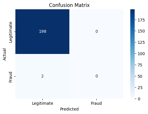
Confusion Matrix:
[[198   0]
 [  2   0]]

C:\ProgramData\anaconda3\envs\mlpy\lib\site-packages\sklearn\metrics\_classification.py:1334: UndefinedMetricWarning: Precision is ill-defined and being set to 0.0 due to no predicted samples. Use `zero_division` parameter to control this behavior.
  _warn_prf(average, modifier, msg_start, len(result))

#!pip install seaborn

import matplotlib.pyplot as plt
import seaborn as sns

# Plot confusion matrix
plt.figure(figsize=(6,4))
sns.heatmap(conf_matrix, annot=True, fmt='d', cmap='Blues',
            xticklabels=['Legitimate', 'Fraud'],
            yticklabels=['Legitimate', 'Fraud'])
plt.ylabel('Actual')
plt.xlabel('Predicted')
plt.title('Confusion Matrix')
plt.show()

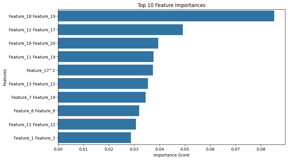
# Feature importance
importances = rf.feature_importances_
feature_names_final = X.columns
feature_importance = pd.Series(importances, index=feature_names_final).sort_values(ascending=False)

# Plot top 10 feature importances
plt.figure(figsize=(10,6))
sns.barplot(x=feature_importance[:10], y=feature_importance[:10].index)
plt.title('Top 10 Feature Importances')
plt.xlabel('Importance Score')
plt.ylabel('Features')
plt.show()

_images/461977e20a12c0de40a6d8e80217edf43a39acc57741630cd0e3070f144a820d.png

_images/b772e4784cb2814d245ecab6404e185f1ac46376482af425d5e6ce847ec3ad01.png

pip install docutils==0.18

pip uninstall docutils

Financial Fraud Detection

Contents

Financial Fraud Detection#

1. Introduction#

2. Types of Financial Fraud#

2.1. Transaction Fraud#

2.2. Identity-Related Fraud#

2.3. Internal Fraud#

2.4. Cyber-Fraud#

2.5. Advanced and Emerging Fraud Types#

3. Methods Used in Literature for Fraud Detection#

3.1. Supervised Learning Methods#

3.2. Unsupervised Learning Methods#

3.3. Semi-Supervised and Reinforcement Learning Methods#

3.4. Hybrid and Ensemble Methods#

3.5. Emerging and Advanced Methods#

4. Evaluation Metrics Used in Fraud Detection#

4.1. Accuracy#

4.2. Precision#

4.3. Recall/Sensitivity/True Positive Rate (TPR)#

4.4. F-measure (F1 Score)#

4.5. Specificity (True Negative Rate, TNR)#

4.6. Area Under the Receiver Operating Characteristic Curve (AUC-ROC)#

4.7. Matthews Correlation Coefficient (MCC)#

4.8. Cost-Based Metrics#

4.9. Precision-Recall Curve#

5. Common Challenges in Financial Fraud Detection#

5.1. Imbalanced Datasets#

5.2. Data/Concept Drift#

5.3. Feature Selection and Engineering#

5.4. Scalability and Real-Time Detection#

5.5. Interpretability and Explainability#

5.6. Data Privacy and Security#

5.7. High False Positive Rates#

6. Innovative Approaches: Financial Fraud Detection Using Quantum Graph Neural Networks#

6.1. Overview#

6.2. Key Contributions#

6.3. Implications and Future Directions#

Create feature names#

Create DataFrame#

Display class distribution#