Risk Minimization#
#!pip install numpy pandas scikit-learn xgboost matplotlib seaborn
import numpy as np
import pandas as pd

# Set a random seed for reproducibility
np.random.seed(42)

# Number of samples
n_samples = 1000

# Generate ovd_days (overdue days)
ovd_days = np.random.randint(0, 120, size=n_samples)

# Generate ovd30, ovd60, ovd90 based on ovd_days
ovd30 = np.where(ovd_days >= 30, np.random.uniform(100, 1000, size=n_samples), 0)
ovd60 = np.where(ovd_days >= 60, np.random.uniform(100, 1000, size=n_samples), 0)
ovd90 = np.where(ovd_days >= 90, np.random.uniform(100, 1000, size=n_samples), 0)

# Generate additional 16 features (e.g., income, age, credit score, etc.)
additional_features = {
    f'feature_{i}': np.random.uniform(0, 1, size=n_samples)
    for i in range(1, 17)
}

# Define the target variable 'default'
default = np.where(ovd_days >= 90, 1, 0)

# Create a DataFrame
data = pd.DataFrame({
    'ovd_days': ovd_days,
    'ovd30': ovd30,
    'ovd60': ovd60,
    'ovd90': ovd90,
    'default': default
})

# Add additional features to the DataFrame
for feature_name, values in additional_features.items():
    data[feature_name] = values

# Display the first few rows
print(data.head())
   ovd_days       ovd30       ovd60       ovd90  default  feature_1  \
0       102  347.258617  365.750460  828.264854        1   0.170115
1        51  286.504884    0.000000    0.000000        0   0.898238
2        92  890.398601  266.705602  730.030845        1   0.776803
3        14    0.000000    0.000000    0.000000        0   0.076480
4       106  142.206821  482.074683  459.190169        1   0.986729

   feature_2  feature_3  feature_4  feature_5  ...  feature_7  feature_8  \
0   0.772671   0.910665   0.970555   0.874897  ...   0.210387   0.825302
1   0.714900   0.435672   0.558953   0.771783  ...   0.290295   0.066410
2   0.578978   0.129086   0.336394   0.417907  ...   0.786544   0.170860
3   0.014609   0.742299   0.519022   0.748406  ...   0.159390   0.311121
4   0.360375   0.643104   0.979263   0.961335  ...   0.044092   0.320699

   feature_9  feature_10  feature_11  feature_12  feature_13  feature_14  \
0   0.452029    0.665473    0.268009    0.653720    0.697315    0.424151
1   0.101968    0.616738    0.053777    0.278180    0.597098    0.242181
2   0.073059    0.625900    0.924372    0.472927    0.488936    0.327334
3   0.462255    0.296270    0.661721    0.846581    0.665769    0.985358
4   0.301597    0.415145    0.886623    0.335464    0.371363    0.368168

   feature_15  feature_16
0    0.601807    0.902878
1    0.130799    0.234079
2    0.582533    0.547901
3    0.088851    0.707345
4    0.490584    0.271884

[5 rows x 21 columns]
import matplotlib.pyplot as plt
import seaborn as sns

# Check for missing values
print("Missing values in each column:")
print(data.isnull().sum())

# Distribution of the target variable
sns.countplot(x='default', data=data)
plt.title('Distribution of Default Variable')
plt.show()

# Correlation heatmap
plt.figure(figsize=(12, 10))
sns.heatmap(data.corr(), cmap='coolwarm', annot=False)
plt.title('Correlation Heatmap')
plt.show()
---------------------------------------------------------------------------
ModuleNotFoundError                       Traceback (most recent call last)
Cell In[3], line 2
      1 import matplotlib.pyplot as plt
----> 2 import seaborn as sns
      4 # Check for missing values
      5 print("Missing values in each column:")

ModuleNotFoundError: No module named 'seaborn'
# Data Pre-processing
from sklearn.preprocessing import StandardScaler

# Separate features and target
X = data.drop('default', axis=1)
y = data['default']

# Feature Scaling
scaler = StandardScaler()
X_scaled = scaler.fit_transform(X)
# Split the dataset into training and testing sets.
from sklearn.model_selection import train_test_split

# Split the data (80% training, 20% testing)
X_train, X_test, y_train, y_test = train_test_split(
    X_scaled, y, test_size=0.2, random_state=42
)
# !pip install xgboost
# building the model
import xgboost as xgb
from xgboost import XGBClassifier

# Initialize the model
model = XGBClassifier(
    n_estimators=100,
    learning_rate=0.1,
    max_depth=5,
    random_state=42,
    # use_label_encoder=False,
    eval_metric='logloss'
)

# Train the model
model.fit(X_train, y_train)
XGBClassifier(base_score=None, booster=None, callbacks=None,
              colsample_bylevel=None, colsample_bynode=None,
              colsample_bytree=None, device=None, early_stopping_rounds=None,
              enable_categorical=False, eval_metric='logloss',
              feature_types=None, gamma=None, grow_policy=None,
              importance_type=None, interaction_constraints=None,
              learning_rate=0.1, max_bin=None, max_cat_threshold=None,
              max_cat_to_onehot=None, max_delta_step=None, max_depth=5,
              max_leaves=None, min_child_weight=None, missing=nan,
              monotone_constraints=None, multi_strategy=None, n_estimators=100,
              n_jobs=None, num_parallel_tree=None, random_state=42, ...)
In a Jupyter environment, please rerun this cell to show the HTML representation or trust the notebook. On GitHub, the HTML representation is unable to render, please try loading this page with nbviewer.org.
XGBClassifier(base_score=None, booster=None, callbacks=None,
              colsample_bylevel=None, colsample_bynode=None,
              colsample_bytree=None, device=None, early_stopping_rounds=None,
              enable_categorical=False, eval_metric='logloss',
              feature_types=None, gamma=None, grow_policy=None,
              importance_type=None, interaction_constraints=None,
              learning_rate=0.1, max_bin=None, max_cat_threshold=None,
              max_cat_to_onehot=None, max_delta_step=None, max_depth=5,
              max_leaves=None, min_child_weight=None, missing=nan,
              monotone_constraints=None, multi_strategy=None, n_estimators=100,
              n_jobs=None, num_parallel_tree=None, random_state=42, ...)
from sklearn.metrics import (
accuracy_score, confusion_matrix, classification_report, roc_auc_score, roc_curve
)
# Predictions on the test set
y_pred = model.predict(X_test)
y_pred_proba = model.predict_proba(X_test)[:, 1]
# Accuracy
accuracy = accuracy_score(y_test, y_pred)
print(f'Accuracy: {accuracy:.2f}')
# Confusion Matrix
cm = confusion_matrix(y_test, y_pred)
sns.heatmap(cm, annot=True, fmt='d')
plt.title('Confusion Matrix')
plt.xlabel('Predicted')
plt.ylabel('Actual')
plt.show()
# Classification Report
print('Classification Report:')
print(classification_report(y_test, y_pred))
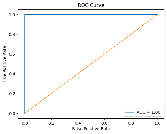
# ROC AUC Score
roc_auc = roc_auc_score(y_test, y_pred_proba)
print(f'ROC AUC Score: {roc_auc:.2f}')
# ROC Curve
fpr, tpr, thresholds = roc_curve(y_test, y_pred_proba)
plt.plot(fpr, tpr, label=f'AUC = {roc_auc:.2f}')
plt.plot([0, 1], [0, 1], linestyle='--')
plt.title('ROC Curve')
plt.xlabel('False Positive Rate')
plt.ylabel('True Positive Rate')
plt.legend()
plt.show()
Accuracy: 1.00
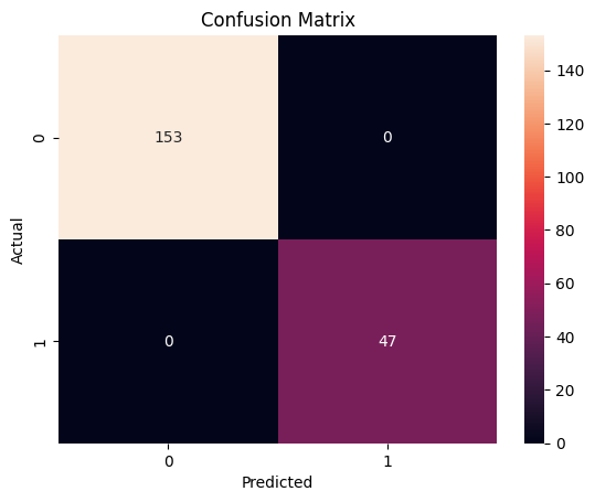
Classification Report:
              precision    recall  f1-score   support

           0       1.00      1.00      1.00       153
           1       1.00      1.00      1.00        47

    accuracy                           1.00       200
   macro avg       1.00      1.00      1.00       200
weighted avg       1.00      1.00      1.00       200

ROC AUC Score: 1.00
Model Comparisons#
import numpy as np
import pandas as pd
from sklearn.model_selection import train_test_split
import warnings
warnings.filterwarnings('ignore')

# Generate synthetic data
np.random.seed(42)
n_samples = 1000
ovd_days = np.random.randint(0, 120, size=n_samples)
ovd30 = np.where(ovd_days >= 30, np.random.uniform(100, 1000, size=n_samples), 0)
ovd60 = np.where(ovd_days >= 60, np.random.uniform(100, 1000, size=n_samples), 0)
ovd90 = np.where(ovd_days >= 90, np.random.uniform(100, 1000, size=n_samples), 0)
additional_features = {f'feature_{i}': np.random.uniform(0, 1, size=n_samples) for i in range(1, 17)}
default = np.where(ovd_days >= 90, 1, 0)

# Create DataFrame
data = pd.DataFrame({'ovd_days': ovd_days, 'ovd30': ovd30, 'ovd60': ovd60, 'ovd90': ovd90, 'default': default})
for feature_name, values in additional_features.items():
    data[feature_name] = values

# Splitting data into train, validation, and holdout sets
X = data.drop('default', axis=1)
y = data['default']

# Train-Validation-Holdout split (60-20-20)
X_train_full, X_holdout, y_train_full, y_holdout = train_test_split(X, y, test_size=0.2, random_state=42)
X_train, X_val, y_train, y_val = train_test_split(X_train_full, y_train_full, test_size=0.25, random_state=42)  # 0.25 x 0.8 = 0.2

print(f"Training set size: {X_train.shape[0]}")
print(f"Validation set size: {X_val.shape[0]}")
print(f"Holdout set size: {X_holdout.shape[0]}")
Training set size: 600
Validation set size: 200
Holdout set size: 200
#!pip install catboost
# Indivudal Models
from sklearn.linear_model import LogisticRegression
from sklearn.tree import DecisionTreeClassifier
from sklearn.ensemble import RandomForestClassifier
import xgboost as xgb
import lightgbm as lgb
from catboost import CatBoostClassifier

# Instantiate individual models
logistic_model = LogisticRegression(random_state=42)
decision_tree = DecisionTreeClassifier(random_state=42)
random_forest = RandomForestClassifier(n_estimators=100, random_state=42)
xgboost_model = xgb.XGBClassifier(n_estimators=100, learning_rate=0.1, max_depth=5, random_state=42, eval_metric='logloss')
lightgbm_model = lgb.LGBMClassifier(n_estimators=100, learning_rate=0.1, max_depth=5, random_state=42)
catboost_model = CatBoostClassifier(n_estimators=100, learning_rate=0.1, max_depth=5, random_state=42, verbose=0)
# Stacking
# For stacking, we will combine the predictions of individual models using a meta-model.
from sklearn.ensemble import StackingClassifier

# Define base models for stacking
base_models = [
    ('logistic', logistic_model),
    ('decision_tree', decision_tree),
    ('random_forest', random_forest),
    ('xgboost', xgboost_model),
    ('lightgbm', lightgbm_model),
    ('catboost', catboost_model)
]

# Meta-model: Logistic Regression
meta_model = LogisticRegression(random_state=42)

# Stacking Classifier
stacking_model = StackingClassifier(estimators=base_models, final_estimator=meta_model, cv=5)
# Training all models
models = {
    "Logistic Regression": logistic_model,
    "Decision Tree": decision_tree,
    "Random Forest": random_forest,
    "XGBoost": xgboost_model,
    "LightGBM": lightgbm_model.set_params(verbose=-1),  # Set verbose to -1 to silence output
    "CatBoost": catboost_model,
    "Stacking Model": stacking_model
}

# Train each model on the training set
for name, model in models.items():
    print(f"Training {name}...")
    model.fit(X_train, y_train)
Training Logistic Regression...
Training Decision Tree...
Training Random Forest...
Training XGBoost...
Training LightGBM...
Training CatBoost...
Training Stacking Model...
# !pip install ace_tools
from sklearn.metrics import accuracy_score, roc_auc_score, precision_score, recall_score

def evaluate_model(model, X, y):
    """
    Evaluate the model on the given dataset and return various performance metrics.

    Parameters:
    - model: Trained model to evaluate
    - X: Feature matrix
    - y: True labels

    Returns:
    - accuracy: Accuracy score of the model
    - roc_auc: ROC AUC score
    - precision: Precision score
    - recall: Recall score
    """
    predictions = model.predict(X)
    proba = model.predict_proba(X)[:, 1]  # Probability estimates for the positive class
    accuracy = accuracy_score(y, predictions)
    roc_auc = roc_auc_score(y, proba)
    precision = precision_score(y, predictions)
    recall = recall_score(y, predictions)
    return accuracy, roc_auc, precision, recall

# Evaluating models on the validation set
validation_results = pd.DataFrame(columns=["Model", "Accuracy", "ROC AUC", "Precision", "Recall"])

for name, model in models.items():
    accuracy, roc_auc, precision, recall = evaluate_model(model, X_val, y_val)
    result = pd.DataFrame({
        "Model": [name],
        "Accuracy": [accuracy],
        "ROC AUC": [roc_auc],
        "Precision": [precision],
        "Recall": [recall]
    })
    validation_results = pd.concat([validation_results, result], ignore_index=True)


# Evaluate each model on the holdout set
holdout_results = pd.DataFrame(columns=["Model", "Accuracy", "ROC AUC", "Precision", "Recall"])

for name, model in models.items():
    accuracy, roc_auc, precision, recall = evaluate_model(model, X_holdout, y_holdout)
    result = pd.DataFrame({
        "Model": [name],
        "Accuracy": [accuracy],
        "ROC AUC": [roc_auc],
        "Precision": [precision],
        "Recall": [recall]
    })
    holdout_results = pd.concat([holdout_results, result], ignore_index=True)

# Display holdout results
print(holdout_results)
                 Model  Accuracy  ROC AUC  Precision  Recall
0  Logistic Regression       1.0      1.0        1.0     1.0
1        Decision Tree       1.0      1.0        1.0     1.0
2        Random Forest       1.0      1.0        1.0     1.0
3              XGBoost       1.0      1.0        1.0     1.0
4             LightGBM       1.0      1.0        1.0     1.0
5             CatBoost       1.0      1.0        1.0     1.0
6       Stacking Model       1.0      1.0        1.0     1.0