flowchart TD
  I["Intervention on a choice from<br/>menu C with attributes x_j<br/>and prices p_j"] --> PC["Price cut or<br/>quality improvement"]
  I --> BN["Ban"]
  I --> ND["Nudge"]
  PC --> PC2["Changes V through<br/>p_j or x_j:<br/>economic incentives"]
  BN --> BN2["Deletes option j<br/>from the menu C"]
  ND --> ND2["Adds γ·d_j(a):<br/>default status, list rank,<br/>salience weight"]
  ND2 --> ND3["Menu and prices intact;<br/>under neoclassical axioms γ = 0"]
20 Nudges and Choice Architecture
Every choice a consumer faces arrives wrapped in a context: an order in which options appear, a pre-checked box, a number printed on a label, a sentence that frames the same outcome as a gain or a loss. None of these features alters the underlying options, yet each reliably moves what people choose. A choice architect is anyone who organizes the context in which decisions are made—the designer of an enrollment form, the merchandiser who sets a shelf, the platform engineer who selects a default. A nudge is any aspect of that architecture that predictably changes behavior without forbidding options or materially changing economic incentives. The defining feature is that the intervention is cheap to avoid: a true nudge leaves the menu and the prices intact and works through how the choice is presented, not through what is on offer.
This chapter treats choice architecture as both a scientific object and a managerial instrument. Scientifically, nudges are where the behavioral-economics account of the consumer—bounded rationality, reference dependence, present bias, sensitivity to social information—meets the firm’s ability to engineer the environment. Commercially, the same levers that a public-health agency uses to raise organ-donor registration are the levers a retailer uses to raise basket size, and the line between a welfare-improving nudge and an exploitative “dark pattern” is drawn by whose objective the architecture serves. We therefore give equal weight to mechanism (why defaults, framing, social proof, and salience work), to measurement (how field experiments identify a nudge effect and what breaks that identification), and to ethics and welfare (when steering a chooser is legitimate). By the end the reader should be able to formalize a nudge as a shift in a choice model, design a field test that recovers its causal effect, and reason explicitly about the welfare claim that justifies it.
The intellectual debt is to the heuristics-and-biases program—the systematic departures from expected-utility maximization catalogued by A. Tversky and Kahneman (1974) and A. Tversky and Kahneman (1981)—and to the reference-dependent account of value in R. Thaler (1985). The managerial program that builds on it, libertarian paternalism, holds that because choices are never presented context-free, the architect cannot avoid influencing behavior; the only question is whether that influence is exercised thoughtfully and in the chooser’s interest.1 We adopt that framing while treating the welfare claim as something to be argued, not assumed.
20.1 Theoretical Foundations
Choice architecture has no force of its own; it works only because human choice departs from the rational-agent benchmark in regular, theorized ways. The governing lens is behavioral economics, and each core lever in this chapter is a deployment of a specific behavioral-economic theory. Naming those theories makes the mechanism explicit and the welfare argument auditable.
The foundation is prospect theory (Kahneman and Tversky 1979; A. Tversky and Kahneman 1981). People evaluate outcomes as gains and losses relative to a reference point, with a value function that is steeper for losses than for equivalent gains. This single idea underwrites two levers at once. It explains framing: relabeling the reference point (the “90% lean” versus “10% fat” contrast) changes valuation even though the final state is identical, because the loss-averse chooser is not invariant to the reference the way a final-wealth maximizer would be. It also explains the stickiness of defaults through status-quo bias, the riskless-choice form of reference dependence in which moving away from the inherited option registers as a loss and is therefore resisted (Amos Tversky and Kahneman 1991). The endowment effect (willingness to accept exceeding willingness to pay) is the same asymmetry seen from the side of ownership, and it is why a default, once held, feels costly to surrender.
Three further behavioral-economic theories complete the account. Mental accounting (R. Thaler 1985) holds that consumers code outcomes into separate, non-fungible cognitive accounts, so the partitioning and framing of a cost (an installment versus a lump sum, a fee versus a base price) changes evaluation even when the net economics are unchanged. Salience theory (Bordalo, Gennaioli, and Shleifer 2013) formalizes limited attention: decision weights are distorted toward whatever stands out in the choice context, which is exactly the primitive a salience nudge perturbs (a calorie label, a conspicuous fee). And present bias, the hyperbolic-discounting result that near-term outcomes are over-weighted relative to the long term (Laibson 1997), explains why people under-save, procrastinate cancellation, and impulse-buy: it is the time-preference failure that automatic enrollment and commitment-style nudges are designed to correct. Social norms supply the final primitive: descriptive and injunctive norms move behavior, often more than people predict, which is the engine of every social-proof nudge (Cialdini, Reno, and Kallgren 1990; Goldstein, Cialdini, and Griskevicius 2008).
These theories are organized into a managerial program by libertarian paternalism, the framing introduced in Thaler and Sunstein’s Nudge: because choice is never presented context-free, the architect cannot avoid influencing behavior, so the only question is whether that influence is exercised thoughtfully and in the chooser’s interest. The program’s empirical credibility rests on field evidence that defaults and reminders change behavior cheaply at scale (Johnson and Goldstein 2003; Benartzi et al. 2017). Its critics press two objections. The first is normative: the paternalism is real, and the “libertarian” promise of a free opt-out is partly illusory wherever exiting carries even small friction, the concern formalized as sludge, the welfare-reducing mirror of a nudge (R. H. Thaler 2018). The second is empirical: meta-analytic re-readings argue that average nudge effects are smaller and more publication-biased than the headline cases suggest, so the intervention should be sized honestly rather than oversold. We adopt the libertarian-paternalism framing while treating both the welfare claim and the effect size as quantities to be argued and measured, not assumed; Section 20.5 and Section 20.7 take up each in turn.
20.2 What a Nudge Is, Formally
Intuitively, a nudge changes behavior without changing the rational consumer’s problem. To make this precise, consider a chooser selecting from a menu \(\mathcal{C} = \{1,\dots,J\}\) of options, each with attributes \(\mathbf{x}_j\) and price \(p_j\). In the standard random-utility model the chooser selects option \(j\) when its latent utility is largest, \[ U_j = V(\mathbf{x}_j, p_j) + \varepsilon_j, \qquad j^\star = \arg\max_{j \in \mathcal{C}} U_j , \tag{20.1}\] with \(V\) the deterministic (systematic) component and \(\varepsilon_j\) an idiosyncratic shock. A price cut or a quality improvement moves choices by changing \(V\) through \(p_j\) or \(\mathbf{x}_j\). A ban moves choices by deleting \(j\) from \(\mathcal{C}\). A nudge does neither. It is a feature \(a\) of the choice architecture that enters utility (or the choice rule) without changing the menu \(\mathcal{C}\) or the economic terms \((\mathbf{x}_j, p_j)\): \[ \tilde U_j = V(\mathbf{x}_j, p_j) + \gamma\, d_j(a) + \varepsilon_j , \tag{20.2}\] where \(d_j(a)\) encodes how architecture \(a\) touches option \(j\)—an indicator that \(j\) is the default, the rank of \(j\) in a list, the salience weight on \(j\)’s price—and \(\gamma\) is the behavioral sensitivity. Under the neoclassical axioms \(\gamma = 0\): presentation is irrelevant and choice is invariant to anything but \((\mathbf{x}_j, p_j)\). Every nudge is, in this notation, a claim that \(\gamma \neq 0\) for some architecture-dependent term that a fully rational agent would ignore. Figure 20.1 locates the nudge among the interventions available to anyone who shapes a choice: it alone moves behavior while leaving both the menu and the economic terms intact.
A nudge is any aspect of the choice architecture that alters people’s behavior in a predictable way without forbidding any options or significantly changing their economic incentives. To count as a mere nudge, the intervention must be easy and cheap to avoid.
— after the standard definition in the libertarian-paternalism literature
Two corollaries follow and discipline the rest of the chapter. First, because the nudge operates through \(\gamma\, d_j(a)\) rather than through preferences, its effect is a property of the interaction between the architecture and the population’s behavioral parameters—the same default can be inert in one segment and decisive in another (Section 20.4). Second, the welfare evaluation of a nudge cannot be read off revealed choice in the usual way: if \(\gamma \neq 0\), the option chosen under architecture \(a\) need not be the one that maximizes the chooser’s experienced utility, so the architect must invoke a welfare criterion external to the choice itself (Section 20.5).
It is useful to separate two channels by which \(d_j(a)\) can act, because they imply different robustness and different ethics. A nudge may supply information or structure that a rational but cognitively limited agent would want—reducing search cost, correcting a misperception, making a consequence vivid—in which case it moves choice toward what the agent would pick on reflection. Or it may exploit a bias—anchoring on an arbitrary number, triggering loss aversion, leveraging inertia—in which case it moves choice toward what the architect wants regardless of the chooser’s interest. The same formal object, \(\gamma\, d_j(a)\), covers both; the welfare sign is not in the math but in the mapping from the manipulated choice to the chooser’s own ends.
Even within the bias-exploiting channel, force is not guaranteed. The arbitrary-number anchoring that folklore treats as universal is, across fifty years of evidence, among the weakest forms: meta-analyzing more than 2,600 effect sizes, Schley and Weingarten (2026) find that incidental and random-number anchors show much smaller and sometimes null effects once incentives or debiasing enter, while informative anchors stay robust (Hedges’ \(g \approx 0.83\)). Naming a mechanism does not certify that a nudge will move anyone—an empirical caution the boundary-conditions discussion later in the chapter develops.
Controversy: how big is a nudge, really?
The aggregate effectiveness of choice architecture has been contested in print since 2022, and the dispute is as much about meta-analytic method as about nudges. It is a useful case precisely because all parties are looking at overlapping evidence.
2022 — the pooled estimate. Mertens et al. (2022) publish The Effectiveness of Nudging: A Meta-Analysis of Choice Architecture Interventions Across Behavioral Domains in PNAS, reporting a moderate positive average effect.
2022 — two reanalyses, same journal, same year. The replies do not bury their conclusions in the abstract. Maier et al. (2022) is titled No Evidence for Nudging After Adjusting for Publication Bias: reanalyzing the same evidence with bias corrections, they report an average effect not distinguishable from zero. Szaszi et al. (2022) is titled No Reason to Expect Large and Consistent Effects of Nudge Interventions, and raises a different objection—the heterogeneity across interventions is so large that a pooled average is not the right summary object at all.
Three papers, one journal, one year, and the disagreement stated in the titles. This is the fastest published exchange in the set of controversies this book documents, and the speed is a function of format: PNAS accommodates short letters, so a reanalysis can appear while the original is still news, rather than the decade-long lags typical of the marketing exchanges in Section 78.5.
Where it rests. These are not reconcilable by collecting more studies, because the disagreement is about what to do with the studies already collected—specifically, how aggressively to correct for the fact that null nudge results are less likely to be published, and whether averaging across heterogeneous interventions produces a number that means anything. Both are live methodological questions in every applied meta-analysis, not just this one.
The practical reading for someone designing a nudge is that neither “nudges work” nor “nudges do not work” is a claim the evidence supports at that level of generality. The useful questions are which lever, in which population, against which baseline—which is how the rest of this chapter is organized. Section 78.1 places this exchange within the broader credibility revolution, and Section 4.6.3 shows the same base-rate reasoning applied to a different literature.
20.3 The Core Levers
Four families of nudge recur across domains because each maps onto a robust regularity in how people depart from Equation 20.1. Table 20.1 organizes them by the behavioral primitive each exploits, the formal object it perturbs, and the canonical field application. We then treat each in turn.
| Lever | Behavioral primitive | What it perturbs in Equation 20.2 | Canonical application |
|---|---|---|---|
| Default | Status-quo bias, inertia, effort cost | Sets \(d_j(a)=1\) for the opt-out option | Auto-enrollment in retirement saving; organ donation |
| Framing | Reference dependence, loss aversion | Relabels the reference point in \(V\) | “90% lean” vs. “10% fat”; gain/loss appeals |
| Social proof | Conformity, descriptive norms | Adds a term in others’ choices to \(V\) | “Most guests reuse their towels”; energy reports |
| Salience | Limited attention, fluency | Reweights an attribute already in \(V\) | Calorie labels; “sale” tags; traffic-light nutrition |
20.3.1 Defaults
A default is the outcome that obtains when the chooser does nothing. Defaults are the most powerful nudge because doing nothing is the cheapest action: any positive cost of deliberation, comprehension, or execution makes the pre-set option disproportionately likely to stand. Formally, let the chooser realize the default \(j_0\) unless she pays an idiosyncratic switching cost \(c_i\) to move, choosing to switch only when the utility gain exceeds that cost, \[ \Pr(\text{switch from } j_0 \text{ to } j) = \Pr\!\big(U_{ij} - U_{ij_0} > c_i\big). \tag{20.3}\] When \(c_i\) is small the default barely matters; when \(c_i\) is large—or when the chooser never engages the comparison at all because attention is itself costly—the default captures nearly the whole market. Three forces inflate the effective \(c_i\): inertia (status-quo bias, an instance of loss aversion in which moving away from the reference point registers as a loss), implied endorsement (the chooser reads the default as the architect’s recommendation), and effort (comprehending and executing a change has real cognitive and procedural cost). The celebrated cross-country contrast in organ-donor rates—near universal registration under opt-out regimes, sparse registration under opt-in, holding stated attitudes roughly constant—is the limiting case in which \(c_i\) dominates the modest utility difference between registering and not (Johnson and Goldstein 2003). Figure 20.2 traces the process by which the pre-set option becomes the outcome.
flowchart TD
  J0["Default j0 pre-set:<br/>obtains if the chooser<br/>does nothing"] --> AT{"Does the chooser engage<br/>the comparison at all?<br/>(attention is costly)"}
  AT -->|"no"| ST["Default stands"]
  AT -->|"yes"| SW{"Utility gain from switching<br/>greater than cost c_i?"}
  SW -->|"no"| ST
  SW -->|"yes"| MV["Chooser switches to j"]
  F1["Inertia:<br/>status-quo bias,<br/>loss aversion"] --> CI["Forces that inflate c_i"]
  F2["Implied endorsement:<br/>default read as the<br/>architect's recommendation"] --> CI
  F3["Effort:<br/>cognitive and<br/>procedural cost"] --> CI
  CI -.-> SW
The same mechanism drives the marquee result in household finance: automatic enrollment in defined-contribution retirement plans raises participation sharply and persistently, because the inattentive employee inherits the saving rate and fund the plan sets rather than the one she would choose on reflection. Madrian and Shea (2001) document the magnitude: switching a plan default from opt-in to opt-out raised participation from roughly half to more than four-fifths, with most enrollees then anchored on the default contribution rate and fund. R. H. Thaler and Benartzi (2004) turn the same insight into a designed instrument, pre-committing employees to raise contributions out of future raises. That defaults can remedy under-saving is non-trivial precisely because under-saving is itself partly a behavioral failure: Garbinsky, Mead, and Gregg (2020) show that many people save too little not from rational impatience but from a positive illusion of financial responsibility—they believe themselves more financially responsible than the average person, and that flattering self-view dampens the felt need to save. A default that raises the saving rate works with the grain of what these consumers would, on reflection, endorse, which is part of why it is defensible on welfare grounds.
Defaults are not uniformly benign. The identical inertia that lifts retirement saving also sustains negative-option marketing: a free trial that silently converts to a paid subscription, or a pre-checked add-on at checkout, harvests the same \(c_i\) for the firm’s benefit rather than the chooser’s. The welfare sign of a default thus depends entirely on whether the pre-set option is the one the chooser would choose with full attention—a question the architecture is designed to prevent her from confronting.
20.3.2 Framing
A frame is a description of options that is logically equivalent across versions but psychologically distinct. Framing effects are the direct empirical signature of the reference dependence in prospect theory: because the value function is defined over gains and losses relative to a reference point rather than over final states, and is steeper for losses than for equivalent gains, the same outcome described as a loss looms larger than when described as a gain (A. Tversky and Kahneman 1981; R. Thaler 1985). Write the chooser’s valuation as reference-dependent, \[ V_j = v\!\big(\mathbf{x}_j - \mathbf{r}\big), \qquad v'(z) > 0,\quad v''(z) < 0 \text{ for } z>0,\quad v'(0^-) > v'(0^+), \tag{20.4}\] where \(\mathbf{r}\) is the reference point and the last inequality—the kink at zero—is loss aversion. A frame is an intervention on \(\mathbf{r}\): describing ground beef as “90% lean” sets the reference at the favorable attribute, while “10% fat” sets it at the unfavorable one, even though the product is identical. The neoclassical chooser, valuing final states, is invariant to \(\mathbf{r}\) and hence to the frame; the loss-averse chooser is not.
Framing pervades marketing communication. Attribute frames recolor evaluation of a fixed product; goal frames cast the same action as avoiding a loss or securing a gain, with loss frames typically more motivating for prevention behaviors. The “buy now, pay later” (BNPL) instrument studied by Maesen and Ang (2024) is, in part, a framing device: splitting a price into interest-free installments reframes the reference point for the expenditure, and the authors show with retailer transaction data (in a difference-in-differences design around BNPL introduction) and three preregistered experiments that the installment frame reduces perceived financial constraint and perceived cost and improves felt budget control, raising both purchase incidence and basket size relative to lump-sum payment. The effect is concentrated among smaller-basket and credit-reliant shoppers—evidence that the frame bites hardest where the behavioral primitive (here, narrow bracketing of the payment) is strongest, and a reminder that a frame that “helps” budget control can simultaneously raise spending in a way the chooser may not, on reflection, endorse.
20.3.4 Salience
A salience nudge changes which attribute the chooser attends to, without changing the attribute set or the prices. Limited attention means the chooser behaves as if maximizing a distorted utility that overweights whatever is perceptually or cognitively prominent. Let attention weights \(\omega_k \ge 0\) multiply the attributes, \[ \hat V_j = \sum_{k} \omega_k\, \beta_k\, x_{jk}, \qquad \omega_k = \omega_k(\text{salience of attribute } k), \tag{20.6}\] so that a fully attentive chooser has \(\omega_k \equiv 1\) and recovers Equation 20.1, while an inattentive one sets \(\omega_k\) near zero on neglected attributes (a tax not shown at the shelf, a shrouded fee) and above one on prominent ones (a bold “sale” tag, a traffic-light nutrition label). A salience nudge is an intervention on \(\omega_k\): posting calorie counts raises the weight on the health attribute; displaying tax-inclusive prices raises the weight on the true price. Crucially—and unlike framing—a salience nudge can be welfare-improving precisely because it pushes \(\omega_k\) back toward one, undoing a distortion the chooser would not endorse, rather than introducing a new one.
The clean identification of salience effects comes from settings where the information is unchanged but its prominence varies: making an already-disclosed fee conspicuous, or an already-available calorie figure visible at the point of choice, changes behavior even though a rational agent had access to the number all along. Payment form is the canonical demonstration: holding the amount fixed, Soman (2003) shows that more transparent payment mechanisms — those that make the outflow perceptually vivid — depress subsequent spending, which is a pure \(\omega_k\) intervention on an unchanged budget constraint. The same machinery explains why a cost labelled a tax is resisted more than an identical cost labelled a fee or a price (Sussman and Olivola 2011): the label changes the weight, not the arithmetic, which makes it a framing effect with genuine distributional consequences for policy design. Salience is also the lens through which to read “decoy” and assortment effects in Chapter 21 and Chapter 45: adding a dominated option or reordering a shelf reweights attention across an unchanged menu.
Regulators facing shrouded fees have two tools: a salience intervention that raises \(\omega_k\) on the fee (disclosure), and a restriction that removes the fee from the menu (a standardized product). Chile’s consumer-credit reforms let Kulkarni, Truffa, and Iberti (2026) separate them, because standardization and disclosure reached small loans together in 2011 and disclosure alone reached all loans a year later (Section 44.7.1). Disclosure cut delinquency by 13.7 percentage points (40%) and default by 98%; standardization had no effect. Disclosure did not change the terms of the loans borrowers took, so the salience gain showed up after purchase, in repayment, rather than in the choice. An evaluation of a disclosure nudge that looks only at the choice it was meant to inform can therefore miss most of what it does.
20.4 Heterogeneity, Distribution, and the Equity of Nudging
Because a nudge acts through \(\gamma\, d_j(a)\) rather than through preferences, its effect is intrinsically heterogeneous: it is largest for the choosers whose behavioral parameters make them most susceptible and smallest for those who would choose deliberately regardless. This is not a nuisance to be averaged away; it is the policy-relevant heart of the matter, because it determines who a nudge moves and therefore its distributional consequences.
Mrkva et al. (2021) establish this directly: choice-architecture interventions—defaults, attribute ordering, partitioning—have systematically larger effects on consumers with lower socioeconomic status, lower numeracy, and lower domain knowledge. The mechanism is the susceptibility logic above: those with less knowledge or numerical fluency engage the deliberate comparison less and so inherit the architecture more. The distributional implication cuts two ways. A welfare-improving default (auto-enrollment in saving, a healthier cafeteria arrangement) disproportionately helps the disadvantaged and can narrow the gap that arises when the savvy navigate complex choices and the rest default into bad ones. The very same asymmetry means an exploitative architecture disproportionately harms the disadvantaged. Heterogeneity is thus an amplifier whose sign is set by the architect’s objective, and a nudge’s equity case rests on aligning that objective with the interests of the most susceptible.
This connects to the welfare argument that follows: the standard libertarian defense—“opting out is free, so no one is worse off”—is weakest exactly where the nudge is strongest, because the populations least likely to opt out are the least-resourced. The freedom to opt out is not equally distributed.
Heterogeneity can also split which benefits reach whom. Breza, Kanz, and Klapper (2026) ran a field experiment with largely unbanked garment workers in Bangladesh. Wages that had been paid in cash were instead deposited automatically into a bank or mobile-money account, an arrangement that works much like a default: the money arrives in the account unless the worker takes it out. A comparison group received an account but continued to be paid in cash. Exposure to payroll accounts raised account use and sped up learning. Workers built trust in the technology, learned to transact without an agent’s help, and avoided the illicit fees that agents commonly charge inexperienced customers. The effects were concentrated in mobile-money accounts, the newer, more complex, and less trusted of the two technologies. In the working-paper version (Breza, Kanz, and Klapper 2020), a machine-learning search for heterogeneous effects found that the savings gains were broad, but the learning-by-doing gains that protect consumers went mostly to men, to more educated workers, and to those with prior financial access. The same intervention can therefore be progressive in its direct effect and regressive in the learning it induces, and an evaluation that reports only the average savings effect would miss the second distribution entirely.
20.5 Welfare and Ethics
Evaluating a nudge requires a welfare criterion, and revealed preference cannot supply one when \(\gamma \neq 0\). If the architecture itself moves choice, then the chosen option is no longer a clean signal of what the chooser values, and the analyst cannot infer “she chose it, therefore it made her better off.” The behavioral-welfare-economics response is to define welfare relative to the chooser’s preferences as they would be absent the manipulating frame—what she would choose with full attention, no inertia, and a neutral reference point—and to judge a nudge by whether it moves actual choice toward that as-if-rational benchmark. A nudge that closes the gap between distorted and undistorted choice is welfare-improving; one that opens it is not. The difficulty, and it is genuine, is that the undistorted benchmark is partly a construct of the analyst, not an observable.
Three principles operationalize the criterion and double as design tests. First, preserve and cheapen opt-out: the libertarian half of the program is honored only if exiting the default carries trivial cost, and—per Section 20.4—trivial for the least-resourced chooser, not merely for the analyst. Second, publicity: a nudge is more likely legitimate if the architect would be willing to defend it openly to those nudged; covert exploitation of a bias fails this test where transparent information provision passes it. Third, interest alignment: ask whether \(d_j(a)\) steers toward the chooser’s own ends (saving, health, accurate prices) or the architect’s (subscription revenue, larger baskets). The BNPL frame in Maesen and Ang (2024) is instructive here—it improves felt budget control while raising spending, so its welfare sign depends on whether the additional purchases are ones the consumer would endorse on reflection or ones the frame extracts by narrowing attention to the installment.
The adversarial twin of the nudge is the dark pattern: a choice-architecture device engineered to serve the firm at the chooser’s expense—pre-checked add-ons, buried unsubscribe links, drip-priced fees, confirmshaming, manufactured scarcity. Dark patterns are nudges that fail all three tests at once: opt-out is made costly, the design would not survive disclosure, and it steers against the chooser’s interest. The privacy literature documents the analogous machinery in data collection. Adjerid, Acquisti, and Loewenstein (2019) show that consumers’ privacy choices are malleable to framing and to subtle changes in how options are presented, and that the same misdirection that depresses privacy-protective choice can be reversed; Acquisti, John, and Loewenstein (2012) demonstrate that the control a platform appears to grant over disclosure is itself a lever—paradoxically, giving people more nominal control over publication can increase their willingness to disclose sensitive information, a control-as-nudge that benefits the data collector. These are the welfare hard cases: architecture that feels empowering while steering against the chooser’s privacy interest.
Figure 20.3 summarizes the decision the architect actually faces: not whether to architect—context is unavoidable—but whether the architecture they cannot help imposing is aimed at the chooser’s ends or their own.
flowchart TD
    A[Choice architecture<br/>γ·d_j a ≠ 0] --> B{Is opt-out cheap<br/>for the least-resourced chooser?}
    B -- No --> D[Dark pattern]
    B -- Yes --> C{Would the design<br/>survive public disclosure?}
    C -- No --> D
    C -- Yes --> E{Does it steer toward the<br/>chooser's ends or the architect's?}
    E -- Architect's --> D
    E -- Chooser's --> F[Welfare-improving nudge]
    D --> G[Reject / regulate]
    F --> H[Deploy and audit]
20.6 Case: Tip Requests and the Tipping-Culture Debate
Few pieces of choice architecture draw as much public complaint as the tip prompt. Card readers, self-checkout kiosks, delivery apps, and freelance marketplaces now ask for a gratuity where none used to be customary, usually with preset buttons between 15% and 30%, and press coverage has reported customers calling the screens coercive (Kim, Amir, and Wilbur 2026). Critics see the prompt as the dark pattern of Section 20.5: a price increase in disguise, which shifts wage costs onto customers and collects payment through guilt rather than value. Defenders reply that a tip is the one charge only willing buyers pay. On that view it is self-selected price discrimination that keeps posted prices low and rewards effort, and for many gig workers it is a material share of pay (Azar 2020; Kim, Amir, and Wilbur 2026).
Underneath the rhetoric the debate turns on two empirical questions, and both map onto levers from this chapter. Does the wording of the request move behavior, or only the preset amounts (a default)? And when a prompt raises tips, does the platform lose future business, so that a tip behaves like a price increase?
What the default evidence already showed. Haggag and Paci (2014) use a regression discontinuity in New York City taxi payment screens covering more than 13 million rides. Suggested tip defaults have a large effect on tip amounts, but higher suggestions also raise the share of riders who leave no card tip at all. That is the default lever’s opt-out cost made visible. Alexander, Boone, and Lynn (2021) randomize tip recommendations across 94,571 orders from 24,637 customers of an app-based laundry service. The recommendations shift tip amounts but leave satisfaction ratings, return frequency, and bill size unchanged. Interface order matters as well: asking for a rating before the tip lowers tips, because customers feel the rating already rewarded the provider (Chen et al. 2022). None of this work varied the message itself.
The experiment. Kim, Amir, and Wilbur (2026) ran the first large field experiments on tip-request wording, on Fiverr, a global freelance-services marketplace where buyer and seller never meet or speak. After a buyer confirms delivery and rates the gig, the platform shows a tip request with preset amounts. Before the experiment 8% of transactions were tipped, and 70% of tips used a preset button. The web experiment (four weeks from June 10, 2019, persistent randomization at the buyer level) tested four messages:
- Control: “Would you like to leave a tip to [seller name]?”
- Impersonal reciprocity: “Show your appreciation to your seller by giving a tip.”
- Personalized reciprocity: “Leave [seller name] a tip to show your appreciation for a job well done.”
- Injunctive norm: “It’s customary to leave a tip for the seller’s service.”
The norm message is injunctive in the sense of Cialdini, Reno, and Kallgren (1990). It states what buyers ought to do and reports nothing about what most buyers actually do, which would be a descriptive norm and, since actual tipping was rare, would risk the boomerang effect described under Social Proof above.
A confound, and how the authors broke it. The platform’s testing tool allowed only four cells, and management bundled the two stronger messages with a new three-default menu ($5/$10/$15 below a $35 order price, 15%/20%/25% above, versus the old $5/$10 and 20%/30%). As run, the test confounds message with menu. The way out came from what happened afterwards: when the test ended, every arm reverted to the control message but kept the three-default menu. Pooling test and posttest periods gives eight cells, and each message effect is a within-menu contrast. The norm effect compares norm-plus-three-defaults during the test with the control-plus-three-defaults cell that the same arm moved into afterwards, and the menu effect compares the control arm before and after. The design is a regression discontinuity in time layered on a randomized trial. It requires that tipping respond only to the current treatment, that the test dates were set by the firm’s testing calendar rather than by expected business, and that nothing else jumps at the boundary. A donut check that drops the last test week and first posttest week leaves the estimates essentially unchanged. The authors then ran a clean A/B test of the norm message in the mobile app (October 17 to December 10, 2019, 61,705 transactions), with the same three-default menu in both arms. Table 20.2 collects the main estimates.
| Effect on tipping rate (percentage points) | All buyers, first exposure | New buyers, first exposure | Repeat buyers, first exposure | All buyers, all exposures |
|---|---|---|---|---|
| Control tipping rate (web) | 14.8% | 14.6% | 14.9% | 10.6% |
| Impersonal reciprocity | +0.4 (n.s.) | +0.8 (n.s.) | +0.3 (n.s.) | 0.0 (n.s.) |
| Personalized reciprocity | +4.6 | +5.3 | +4.4 | +1.5 |
| Injunctive norm | +7.6 | +11.8 | +6.8 | +3.0 |
| Three-default menu (vs. two) | −4.4 | −4.7 | −4.3 | −1.5 |
| App A/B test: control rate | 8.4% | 9.5% | 8.0% | 7.5% |
| App A/B test: injunctive norm | +1.7 | +2.5 | +1.4 | +1.1 |
Four results bear on the debate. First, wording matters, and the ordering follows theory. The injunctive norm beat personalized reciprocity, and impersonal reciprocity did nothing. Naming the seller seems to be what makes a gratitude appeal work, since it reminds the buyer who earned the thanks. Second, the norm effect is largest for new buyers, who have the least idea what is customary on the platform. Third, the menu change lowered tipping. Adding a $15 button and replacing the 30% option with 15% and 25% pulled tips down, so more options are not automatically a stronger nudge. Fourth, effects grow with order price. In the web test the norm raised first-exposure tipping by 4.6 points on gigs of $10 or less and by 10.9 points above $60; in the app the only large effect was above $60. One reading is that a percentage default loses its pull at high prices, where the tip is expensive enough to be thought through, and an explicit norm takes over that work.
Did tips cost the platform demand? Not detectably, and this is the result that speaks most directly to the “tips are a price increase” side. In the web experiment, buyers assigned the norm message placed about 1.5 more orders and spent about $46 more over the period than control buyers, against a base of roughly 4 orders and $141. The three-default menu reduced orders and spending by similar amounts. In the cleaner app A/B test the norm message had no significant effect on orders or spending in either direction. Readers should hold the web demand numbers loosely. A 36% lift in orders from one sentence on a post-purchase screen is very large, it rests on the pooled test-posttest identification rather than on the randomized contrast alone, and the app test did not reproduce it. The defensible conclusion is the weaker one in the paper’s title: raising tips did not reduce demand. That matches what Alexander, Boone, and Lynn (2021) found for tip recommendations.
What the case does not settle. Even the best arm left most transactions untipped (about 22% of new buyers tipped on first exposure), so one sentence does not create a tipping norm on its own. Only one injunctive message was tested, and the data are from 2019, four years before the 2023 wave of complaints about tip screens that the paper cites. The study observes untipped transactions and repeat purchases but not irritation, guilt, or reactance, so a buyer who kept buying while resenting the prompt counts as no harm. The second author worked part time for Fiverr as a behavioral scientist from 2018 to 2026. The paper discloses this and states that the firm had no right to censor findings. Earlier restaurant studies reviewed in the paper point the other way: an explicit request lowered tips relative to no request, and surveyed customers reported irritation and lower intent to return (Kim, Amir, and Wilbur 2026). Those studies changed whether a request appears; this one changes only its wording once a request is already there.
Running the three welfare tests. The tests from Section 20.5 sort the debate better than the shouting does. Cheap opt-out: declining is one click, and the authors urge platforms to keep tipping fully discretionary; a screen that makes “no tip” hard to find fails here, whatever its wording. Publicity: “It’s customary to leave a tip” states its appeal openly, whereas a pre-selected tip or a guilt-inducing layout would not survive disclosure. Interest alignment is the hard test. Fiverr keeps 20% of seller revenue, tips included, so the platform shares in whatever the prompt raises, and nontippers’ welfare is not measured. The absence of a demand penalty is what separates this prompt from a pure transfer engineered for the architect. Regulation is already in play. New York City requires delivery apps to request tips at or before checkout with a default of at least 10%, and the authors warn that mandating specific defaults or wording without testing could lower workers’ tip income. Given the price-dependent and channel-dependent effects in Table 20.2, that warning is well grounded.
20.7 Identifying a Nudge Effect in the Field
A nudge is a causal claim—\(\gamma \neq 0\) for a specific \(d_j(a)\)—and the gold standard for recovering \(\gamma\) is the randomized field experiment, because laboratory framing effects routinely shrink or vanish under real stakes, deliberation, and repetition. The estimand is the average treatment effect of architecture \(a\) on the choice of interest. With chooser \(i\) randomized to the nudge (\(T_i=1\)) or the status-quo architecture (\(T_i=0\)), and outcome \(Y_i\) (e.g., enrollment, basket size, the share choosing the target option), \[ \tau = \mathbb{E}[Y_i \mid T_i = 1] - \mathbb{E}[Y_i \mid T_i = 0], \tag{20.7}\] identified under randomization by the independence of \(T_i\) from potential outcomes. The estimator is the difference in means (or a regression of \(Y_i\) on \(T_i\) with pre-treatment covariates to soak up residual variance); its assumptions are (i) successful randomization, so treatment is orthogonal to potential outcomes; (ii) the stable-unit-treatment-value assumption (SUTVA)—no interference between units—which a social-proof nudge can threaten precisely because it operates through peers; and (iii) no differential attrition between arms. What breaks identification: spillovers (the nudged and un-nudged talk, or share a shelf), non-compliance (the default is overridden administratively), and outcome measures that capture short-run novelty rather than persistent behavior. The persistence question is first-order for defaults, whose entire value rests on inertia lasting; a one-week bump that decays is not the same asset as auto-enrollment that compounds for decades.
Persistence matters for nudges other than defaults too. A real-time prompt is a salience nudge (Equation 20.6) aimed at one decision, and the obvious worry is that its effect ends with the basket. Gonzálvez et al. (2026) test this with “swap and save” buttons on an online grocery price-comparison platform. The buttons flag a cheaper alternative while the shopper is choosing, and the authors study the mineral water category. Shoppers who switched after a prompt were 23.7 percentage points more likely to choose the alternative again on later visits, and the effect lasted for up to 10 shopping trips. The authors attribute the persistence to product discovery rather than to long-run cost savings: the prompt introduced shoppers to a product they went on to keep buying. This is the state-dependence problem of Section 36.8.9 in nudge form. A shopper who keeps buying the swapped product may have learned something from the prompt, or may be the kind of shopper who would have drifted to it anyway, and a persistence estimate is only as credible as the design that separates the two.
The paper’s online appendix shows how the authors separate them. (The main text was paywalled when this was written, so the 23.7-point headline comes from the abstract and everything below from the appendix.) The data are a year (2015) of item-level purchases on an Israeli price-comparison platform that sits on top of five online supermarkets, merged with a log of every interaction with the swap prompt. In mineral water that is 71,433 purchases by 11,337 shoppers across 38 products. Three layers of evidence follow.
- Matched event study. Each shopper who swapped is matched to a shopper who bought the same initial product at the same supermarket within 30 days and was plausibly never shown the button. That leaves 1,343 treated and 1,762 control shoppers, compared trip by trip around the swap with what the appendix calls a CS DiD, the usual shorthand for Callaway and Sant’Anna (2021). The estimate stays between 20.8 and 27.1 points when the controls are restricted to not-yet-treated shoppers, the matching window shrinks to two days, the sample is cut to infrequent shoppers, or retailer-by-day fixed effects are added. Two placebos come back flat: a fake event three trips before the real one, and a swap in cleaning products as the “treatment” for water.
- Exposure as an instrument. Swappers chose to swap, so the authors widen the sample to everyone who was shown the button, including shoppers who clicked and kept their product and shoppers who never clicked, and instrument swapping with exposure (Section 44.6.4 works through both instruments). Exposure raises the probability of a swap by 36.9 points (first-stage \(F = 890\)), and the IV estimate of the swap’s effect on later purchases of the alternative is 21.4 points, close to the matched estimate. The exclusion restriction is the weak point, because a prompt could work as an advertisement even for shoppers who decline it. The authors check this directly. Exposed shoppers who did not swap are no more likely than controls to buy the alternative later (coefficient \(-0.010\), not significant).
- Stock-outs as a second instrument. When a shopper’s regular water is out of stock, the same button offers in-stock substitutes regardless of price. About half of the shoppers who hit a stock-out swap (first stage 53.5 points, \(F = 136\)), and the forced trial raises later purchases of the substitute by 31.8 points. A trial that has nothing to do with saving money persists at least as strongly as one prompted by a lower price.
The third result, together with the appendix’s price series, is what supports “discovery, not savings.” Price gaps between the commonly swapped pairs move around zero through the year, so the alternative is not reliably cheaper on the next trip, yet shoppers keep buying it. Two measurement choices deserve a reader’s attention. Exposure is inferred for non-clickers (the button was “likely displayed” if someone else triggered a swap on that product, store, and day), and the alternative product for anyone who did not swap is imputed as the most common swap target. Both could blur the instrument, though the first stage is strong enough that weak identification is not the concern. The design is also observational throughout: the platform never randomized the button, so the independence of exposure rests on the argument that day-to-day price movements make the prompt arrive as good as randomly for a given shopper.
When randomization is infeasible because the nudge is rolled out to everyone at once, the workhorse is difference-in-differences (DiD), exactly the design Maesen and Ang (2024) use around the introduction of BNPL. For unit \(i\) in period \(t\), \[ Y_{it} = \alpha_i + \delta_t + \beta\, (\text{Post}_t \times \text{Treated}_i) + \mathbf{z}_{it}^\top\boldsymbol{\gamma} + \varepsilon_{it}, \tag{20.8}\] where \(\alpha_i\) are unit fixed effects, \(\delta_t\) time fixed effects, and \(\beta\) the nudge effect. DiD identifies \(\beta\) under parallel trends: absent the nudge, treated and control units would have moved in parallel. That assumption fails if the nudge is rolled out because the treated group was already trending differently (selection on trends), if a contemporaneous shock hits one group only, or if treatment timing is staggered and effects are heterogeneous across cohorts—the last a now-well-understood pitfall in two-way-fixed-effects estimation. The credible applications buttress parallel trends with pre-period event-study coefficients (flat pre-trends) and placebo outcomes that the nudge should not move. Figure 20.4 summarizes the two identification paths and the assumptions each must defend.
flowchart TD
  CL["Causal claim: γ ≠ 0 for<br/>a specific architecture d_j(a)"] --> RQ{"Can assignment to the<br/>architecture be randomized?"}
  RQ -->|"yes"| RCT["Randomized field experiment:<br/>ATE by difference in means"]
  RQ -->|"no: rolled out to<br/>everyone at once"| DID["Difference-in-differences<br/>around the rollout"]
  RCT --> RA["Must hold: randomization,<br/>SUTVA, no differential attrition"]
  RA --> RB["Breaks: spillovers (social proof),<br/>overridden defaults,<br/>novelty-only outcomes"]
  DID --> PA["Must hold: parallel trends"]
  PA --> PB["Defend with flat pre-trends<br/>(event study) and<br/>placebo outcomes"]
  RB --> PS["Measure persistence:<br/>a default's value pays<br/>only if inertia endures"]
  PB --> PS
The simulation below makes the design concrete and reproducible. We generate a default nudge with a known true effect, embed realistic heterogeneity (the nudge bites harder on low-knowledge choosers, per Mrkva et al. (2021)), and recover the treatment effect by the Equation 20.7 estimator. Figure 20.5 reports the resulting enrollment rates and the sampling distribution of the estimated effect.
Code
set.seed(16)

simulate_nudge_trial <- function(n = 4000,
                                 base_enroll = 0.30,   # opt-in baseline take-up
                                 tau_low = 0.45,       # nudge effect, low-knowledge
                                 tau_high = 0.15) {    # nudge effect, high-knowledge
  # Half the sample is low domain knowledge (more susceptible per Mrkva 2021).
  low_knowledge <- rbinom(n, 1, 0.5)
  treat <- rbinom(n, 1, 0.5)                      # randomized opt-out default
  tau_i <- ifelse(low_knowledge == 1, tau_low, tau_high)
  # Enrollment probability is the baseline plus the (heterogeneous) nudge bump.
  p <- pmin(base_enroll + treat * tau_i, 0.99)
  enroll <- rbinom(n, 1, p)
  data.frame(enroll, treat, low_knowledge)
}

dat <- simulate_nudge_trial()

# Difference-in-means estimator of the ATE (eq-ate).
ate_hat <- mean(dat$enroll[dat$treat == 1]) - mean(dat$enroll[dat$treat == 0])

# Subgroup effects to expose heterogeneity.
sub <- aggregate(enroll ~ treat + low_knowledge, dat, mean)

# Sampling distribution of the estimator across replications.
reps <- replicate(2000, {
  d <- simulate_nudge_trial()
  mean(d$enroll[d$treat == 1]) - mean(d$enroll[d$treat == 0])
})

true_ate <- 0.5 * 0.45 + 0.5 * 0.15   # population-average true effect

op <- par(mfrow = c(1, 2), mar = c(4, 4, 3, 1))

# Panel 1: enrollment by architecture and knowledge.
bar_mat <- matrix(sub$enroll[order(sub$low_knowledge, sub$treat)],
                  nrow = 2,
                  dimnames = list(c("opt-in", "opt-out"),
                                  c("high know.", "low know.")))
barplot(bar_mat, beside = TRUE, ylim = c(0, 1),
        col = c("grey70", "steelblue"),
        ylab = "enrollment rate", main = "Take-up by architecture")
legend("topleft", c("opt-in (status quo)", "opt-out (nudge)"),
       fill = c("grey70", "steelblue"), bty = "n", cex = 0.8)

# Panel 2: sampling distribution of the estimated ATE.
hist(reps, breaks = 30, col = "grey85", border = "white",
     xlab = expression(hat(tau)), main = "Estimated treatment effect")
abline(v = true_ate, lty = 2, lwd = 2)

par(op)

cat("Estimated ATE (single trial): ", round(ate_hat, 3), "\n")
#> Estimated ATE (single trial):  0.292
cat("True population ATE:          ", round(true_ate, 3), "\n")
#> True population ATE:           0.3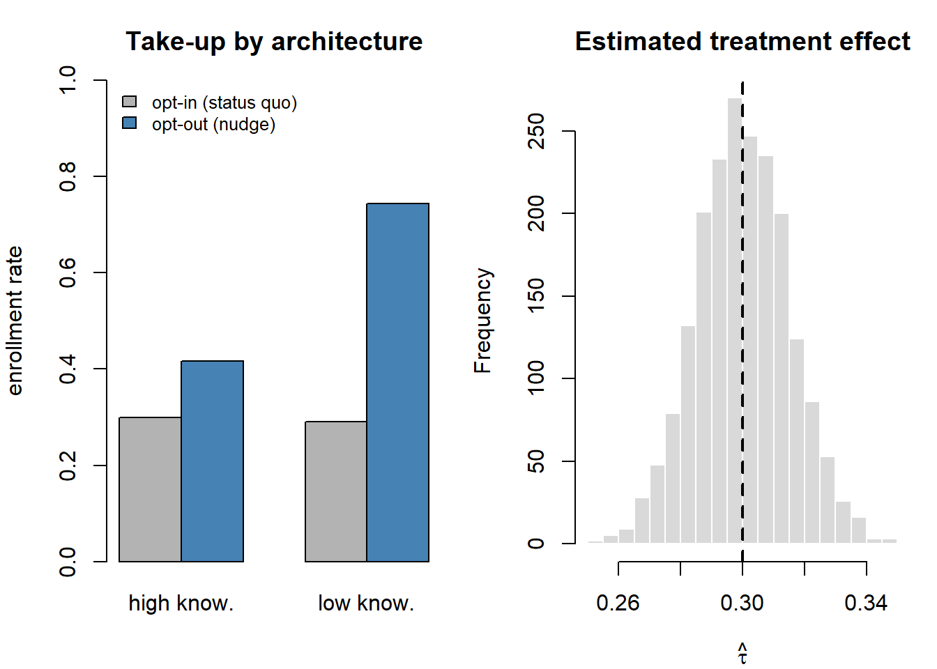
The recovered effect lands on the true population average, and the subgroup panel reproduces the Mrkva et al. (2021) pattern: the same default moves low-knowledge choosers roughly three times as much as high-knowledge ones, the heterogeneity that drives both the equity case and the exploitation risk. Two practical lessons generalize. First, power the experiment for the subgroups that motivate the policy, not just the pooled effect, because the distributional claim is usually the point. Second, measure persistence: re-run the outcome at a horizon long enough to distinguish a durable behavior change from a novelty response, since a default’s value is an annuity that only pays if the inertia endures.
20.8 Pitfalls and Boundary Conditions
Nudges are neither free nor reliably small, and a disciplined account closes with where they fail. Effects decay and are context-bound. A frame that works in one population, at one stake level, with one reference point, often shrinks under real consequences or familiarity; the field-versus-lab gap is the single most common reason a promising laboratory nudge disappoints at scale, which is why Section 20.7 insists on field randomization and persistence measurement rather than one-shot lab demonstrations.
Nudges interact, sometimes destructively. Stacking a default, a social-proof message, and a salience cue is not additive: a descriptive norm can boomerang against above-average performers even as it lifts the rest (Cialdini, Reno, and Kallgren 1990), and a salience nudge that raises attention to one attribute necessarily lowers the relative weight on others (Equation 20.6), so “more salient labels” can crowd out the very dimension a second nudge was meant to promote. The architect optimizes a system of weights, not a list of independent levers.
Reactance and distrust. A nudge perceived as manipulation can trigger reactance, reversing the intended effect and eroding trust in the architect—a risk that scales with how covert the steering is and that the publicity test in Section 20.5 is designed to forestall. Crowding-out of intrinsic motivation is the subtler cousin: a nudge that does the deliberating for the chooser may atrophy the capacity to choose well unaided, a cost invisible in the short-run outcome metric but real over a consumer’s lifetime of decisions. The same reversal reaches explicit incentives, not just presentation: in a natural field experiment, surprise bonuses lowered subsequent effort, the payment read as a signal that the employer was already satisfied rather than a gift to be reciprocated (Bogliacino, Grimalda, and Pipke 2026)—a reminder that an intervention’s effect turns on the meaning the recipient assigns it, not on its size or sign alone.
A long field test shows what separates a small reward that helps from one that backfires. Theory allows either: a token payment can lower effort below no payment at all (Gneezy and Rustichini 2000). Bruers, Ooghe, and Schokkaert (2026) randomized twelve Red Cross-Flanders donation centers to three arms. In the control arm nothing changed. In the second, the monthly newsletter stated the thank-you coupons donors already received: one coupon, worth about €1.50, for a blood donation and two for plasma. The third arm got the same newsletter and, for six months, a third coupon for plasma. The reminder alone raised plasma donations by 4.6% over nine months, but it faded as it was repeated, a decay that a one-shot measurement would miss (Section 20.7). The extra coupon raised plasma donations by a further 7.1%. That effect grew while the coupon was offered and disappeared once it was withdrawn. The dissertation chapter that first reported the experiment finds no drop below the pre-reward level, which is the backlash crowding-out would predict (Bruers 2024). The reward also lowered blood donations at the same centers by 3.3%, so part of the gain was donors switching between two prosocial acts. Earlier work on blood drives found incentives pulling donors away from nearby drives that offered none (Lacetera, Macis, and Slonim 2012). Here the displacement runs across products, which an evaluation that counts only the rewarded behavior cannot see. Survey evidence in the paper suggests that small rewards act as signals of increased need or as gifts that call for reciprocity. That is the same channel as the surprise bonus above: the effect depends on what recipients take the reward to mean, but here the sign is positive. A non-cash gift may also avoid the exchange norms that monetary tokens activate (Yin, Li, and Singh 2020), although the experiment does not compare coupons with cash. Section 76.6.5 reads the paper as a model for framing a simple field experiment.
Removing friction is not always the right move. Sludge analysis treats each added step as a cost (R. H. Thaler 2018), which is correct when the goal is uptake. Dykstra, O’Flaherty, and Whillans (2026) test the case where the goal is use. When the Oregon Department of Transportation moved its carpool platform to a new vendor in 2019, they randomized 27,227 users who had been inactive for six months to two migration emails. In the low-effort arm the account had already been moved and the user only reset a password. In the high-effort arm the user rebuilt the account over three pages, re-entering name, home and work zip codes, and employer (Dykstra, Whillans, and O’Flaherty 2024). Nothing else differed: both arms then had to search for matches and log trips the same way. The harder path lowered sign-ups from 5.1% to 3.8% (694 against 511 people), a 25% drop. Over four months, though, the high-effort arm logged 0.057 more carpool trips per week per person assigned, on a low-effort mean of 0.034, and 5,106 trips in total against 4,311.
The design point is why an intent-to-treat (ITT) gain rules out pure selection. Assignment to the hard path can only remove the “complacent” users who would have signed up only if it were easy, and a removed user contributes zero trips, never a negative number. If the hard path merely filtered out less committed people, total trips in that arm could only stay the same or fall. They rose, so the users who signed up anyway must have carpooled more than they would have after an easy sign-up. A worst-case bound points the same way. Dropping the 25% least active low-effort sign-ups, the share the hard path screened out, shrinks the effect among sign-ups from 1.73 to 1.51 extra trips per week, so selection accounts for some of the effect but not most of it. The effect has limits. At eight months it was about a fifth of its four-month size, and the effect on miles was no longer significant. The October wave alone (10,191 users) was not significant. And the AEA registration was filed after data collection, with the hypotheses fixed earlier in the IRB protocol.
A second experiment, preregistered on Amazon Mechanical Turk with 496 workers (O’Flaherty, Dykstra, and Whillans 2025), made workers who wanted a next-day round of an unpleasant transcription task first answer a 15-question survey about that kind of work. Sign-ups fell only slightly (80.8% to 76.8%, not significant), returns rose from 36.4% to 50.0%, and the effortful arm transcribed 8,438 letters correctly against 5,598. Cross-randomized arms suggest where the effect comes from. A next-day reminder email neither raised returns nor reduced the effort effect, which counts against a memory channel and leaves perceived value as the authors’ preferred reading, though they do not isolate it. Donating the earnings to charity lowered returns by 23 points without changing the effort effect, so the effect does not depend on the task being prosocial.
Three lessons follow for the architect. First, the outcome decides the sign of the effect. A team that scored the carpool test on sign-ups would have dropped the arm that produced the most trips, the same uptake-versus-persistence gap that Section 20.7 warns about. Second, friction is not one quantity with a fixed welfare sign: the authors expect a gain only when the follow-through behavior is voluntary and ongoing and the added step is modest and tied to the goal. Paperwork that only filters people out is the sludge case. Third, the net effect depends on the population. The hard path cost 25% of sign-ups in the field and 5% online, and a population with more complacent users could lose more participation than the remaining users’ extra effort makes up.
Finally, the measurement of welfare remains the binding constraint. Because the undistorted benchmark in Section 20.5 is partly constructed by the analyst, two honest researchers can disagree about a nudge’s sign even given the same effect estimate. The responsible posture is to make the welfare model explicit—state the assumed reference preference, justify it, and report the effect on the susceptible subgroups separately—rather than to let an impressive average treatment effect stand in for a welfare argument it cannot make.
20.9 Key Takeaways
- A nudge changes behavior through the choice architecture (\(\gamma\, d_j(a)\) in Equation 20.2) without altering the menu or the economic terms; under the neoclassical axioms \(\gamma = 0\), so every nudge is a claim that presentation matters where a rational agent would ignore it.
- The four core levers map onto distinct behavioral primitives: defaults exploit inertia (Equation 20.3), framing exploits reference dependence and loss aversion (Equation 20.4), social proof exploits descriptive norms (Equation 20.5), and salience exploits limited attention (Equation 20.6).
- Nudge effects are intrinsically heterogeneous and largest for low-SES, low-numeracy, low-knowledge choosers (Mrkva et al. 2021), so a nudge’s distributional sign is set by the architect’s objective—amplifying help or harm alike.
- Welfare cannot be read off revealed choice when \(\gamma \neq 0\); legitimacy turns on cheap opt-out, surviving public disclosure, and alignment with the chooser’s own ends. Dark patterns are nudges that fail all three.
- Identifying \(\gamma\) in the field means a randomized experiment (Equation 20.7) or a parallel-trends DiD (Equation 20.8), powered for the susceptible subgroups and measured for persistence, not novelty.
20.10 Further Reading
The reference-dependence and heuristics foundations are Kahneman and Tversky (1979), A. Tversky and Kahneman (1974), A. Tversky and Kahneman (1981), Amos Tversky and Kahneman (1991), and R. Thaler (1985); salience and present bias are Bordalo, Gennaioli, and Shleifer (2013) and Laibson (1997); the normative social-influence machinery is Cialdini, Reno, and Kallgren (1990) and Goldstein, Cialdini, and Griskevicius (2008). The choice-architecture program rests on the default evidence of Johnson and Goldstein (2003), the scale evidence of Benartzi et al. (2017), and the sludge counterpoint of R. H. Thaler (2018) (the Nudge monograph of Thaler and Sunstein states the libertarian-paternalism framing in full). For frontier field and behavioral evidence weave the saving-illusion result of Garbinsky, Mead, and Gregg (2020), the choice-architecture-and-inequity result of Mrkva et al. (2021), the BNPL framing evidence of Maesen and Ang (2024), and the privacy choice-architecture work of Adjerid, Acquisti, and Loewenstein (2019) and Acquisti, John, and Loewenstein (2012). For tipping as choice architecture, read Azar (2020) for the economics, Haggag and Paci (2014) and Alexander, Boone, and Lynn (2021) on preset tips, and Kim, Amir, and Wilbur (2026) on request wording (Section 20.6). The construct connects forward to assortment and decoy effects in Chapter 45, price framing in Chapter 21, and the social-evaluation evidence in Chapter 12.
Acquisti, Alessandro, Leslie K John, and George Loewenstein. 2012. “The Impact of Relative Standards on the Propensity to Disclose.” Journal of Marketing Research 49 (2): 160–74.
Adjerid, Idris, Alessandro Acquisti, and George Loewenstein. 2019. “Choice Architecture, Framing, and Cascaded Privacy Choices.” Management Science 65 (5): 2267–90.
Alexander, Damon, Christopher Boone, and Michael Lynn. 2021. “The Effects of Tip Recommendations on Customer Tipping, Satisfaction, Repatronage, and Spending.” Management Science 67 (1): 146–65. https://doi.org/10.1287/mnsc.2019.3541.
Azar, Ofer H. 2020. “The Economics of Tipping.” Journal of Economic Perspectives 34 (2): 215–36. https://doi.org/10.1257/jep.34.2.215.
Benartzi, Shlomo, John Beshears, Katherine L. Milkman, Cass R. Sunstein, Richard H. Thaler, Maya Shankar, Will Tucker-Ray, William J. Congdon, and Steven Galing. 2017. “Should Governments Invest More in Nudging?” Psychological Science 28 (8): 1041–55. https://doi.org/10.1177/0956797617702501.
Bogliacino, Francesco, Gianluca Grimalda, and David Pipke. 2026. “No Gifts Returned: Surprise Bonuses Reduce Productivity in a Natural Field Experiment.” Management Science 72 (7): 5528–43. https://doi.org/10.1287/mnsc.2022.04085.
Bordalo, Pedro, Nicola Gennaioli, and Andrei Shleifer. 2013. “Salience and Consumer Choice.” Journal of Political Economy 121 (5): 803–43. https://doi.org/10.1086/673885.
Bruers, Stijn. 2024. “Selling the Gift of Life? Altruistic Motivation and Monetary Incentives for Blood and Plasma Donations.” {PhD} dissertation, KU Leuven, Faculty of Economics; Business. https://lirias.kuleuven.be/handle/20.500.12942/741809.
Bruers, Stijn, Erwin Ooghe, and Erik Schokkaert. 2026. “The Effect of Small Quasi-Cash Rewards on Prosocial Behavior: The Case of Voluntary Plasma Donations.” Management Science. https://doi.org/10.1287/mnsc.2024.08081.
Callaway, Brantly, and Pedro H. C. Sant’Anna. 2021. “Difference-in-Differences with Multiple Time Periods.” Journal of Econometrics 225 (2): 200–230. https://doi.org/10.1016/j.jeconom.2020.12.001.
Chen, Jinjie, Alison Jing Xu, Maria A. Rodas, and Xuefeng Liu. 2022. “EXPRESS: Order Matters: Rating Service Professionals Reduces Tipping Amount.” Journal of Marketing, April, 002224292210986. https://doi.org/10.1177/00222429221098698.
Cialdini, Robert B., Raymond R. Reno, and Carl A. Kallgren. 1990. “A Focus Theory of Normative Conduct: Recycling the Concept of Norms to Reduce Littering in Public Places.” Journal of Personality and Social Psychology 58 (6): 1015–26. https://doi.org/10.1037/0022-3514.58.6.1015.
Dykstra, Holly, Shibeal O’Flaherty, and Ashley Whillans. 2026. “The Buy-in Effect: When Increasing Initial Effort Encourages Follow-Through.” Management Science. https://doi.org/10.1287/mnsc.2023.03600.
Dykstra, Holly, Ashley Whillans, and Shibeal O’Flaherty. 2024. “The Buy-in Effect: When Increasing Initial Effort Motivates Behavioral Follow-Through.” AEA RCT Registry, AEARCTR-0013133. https://doi.org/10.1257/rct.13133-1.0.
Garbinsky, Emily N., Nicole L. Mead, and Daniel Gregg. 2020. “EXPRESS: Popping the Positive Illusion of Financial Responsibility Can Increase Personal Savings: Applications in Emerging and Western Markets.” Journal of Marketing, November, 002224292097964. https://doi.org/10.1177/0022242920979647.
Gneezy, Uri, and Aldo Rustichini. 2000. “Pay Enough or Don’t Pay at All.” Quarterly Journal of Economics 115 (3): 791–810. https://doi.org/10.1162/003355300554917.
Goldstein, Noah J., Robert B. Cialdini, and Vladas Griskevicius. 2008. “A Room with a Viewpoint: Using Social Norms to Motivate Environmental Conservation in Hotels.” Journal of Consumer Research 35 (3): 472–82. https://doi.org/10.1086/586910.
Gonzálvez, Rubén, Xiaolin Li, Sarit Weisburd, and Xinrong Zhu. 2026. “Swap and Save: How a Button Shapes Lasting Online Grocery Shopping Behavior.” Marketing Science. https://doi.org/10.1287/mksc.2025.0541.
Haggag, Kareem, and Giovanni Paci. 2014. “Default Tips.” American Economic Journal: Applied Economics 6 (3): 1–19. https://doi.org/10.1257/app.6.3.1.
Johnson, Eric J., and Daniel Goldstein. 2003. “Do Defaults Save Lives?” Science 302 (5649): 1338–39. https://doi.org/10.1126/science.1091721.
Kahneman, Daniel, and Amos Tversky. 1979. “Prospect Theory: An Analysis of Decision Under Risk.” Econometrica 47 (2): 263–91. https://doi.org/10.2307/1914185.
Kim, Seung Hyun, On Amir, and Kenneth C. Wilbur. 2026. “Injunctive Norms Outperform Reciprocity: Tip Request Messages Can Increase Tipping Without Reducing Demand.” Marketing Science. https://doi.org/10.1287/mksc.2025.0392.
Kulkarni, Sheisha, Santiago Truffa, and Gonzalo Iberti. 2026. “Removing the Fine Print: Disclosure, Standardized Products, and Consumer Outcomes.” Journal of Financial Economics 185: 104353. https://doi.org/10.1016/j.jfineco.2026.104353.
Lacetera, Nicola, Mario Macis, and Robert Slonim. 2012. “Will There Be Blood? Incentives and Displacement Effects in Pro-Social Behavior.” American Economic Journal: Economic Policy 4 (1): 186–223. https://doi.org/10.1257/pol.4.1.186.
Laibson, David. 1997. “Golden Eggs and Hyperbolic Discounting.” The Quarterly Journal of Economics 112 (2): 443–78. https://doi.org/10.1162/003355397555253.
Madrian, B. C., and D. F. Shea. 2001. “The Power of Suggestion: Inertia in 401(k) Participation and Savings Behavior.” The Quarterly Journal of Economics 116 (4): 1149–87. https://doi.org/10.1162/003355301753265543.
Maesen, S, and D Ang. 2024. “Buy Now Pay Later: Impact of Installment Payments on Customer Purchases.” Journal of Marketing.
Maier, Maximilian, František Bartoš, T. D. Stanley, David R. Shanks, Adam J. L. Harris, and Eric-Jan Wagenmakers. 2022. “No Evidence for Nudging After Adjusting for Publication Bias.” Proceedings of the National Academy of Sciences 119 (31): e2200300119. https://doi.org/10.1073/pnas.2200300119.
Mertens, Stephanie, Mario Herberz, Ulf J. J. Hahnel, and Tobias Brosch. 2022. “The Effectiveness of Nudging: A Meta-Analysis of Choice Architecture Interventions Across Behavioral Domains.” Proceedings of the National Academy of Sciences 119 (1): e2107346118. https://doi.org/10.1073/pnas.2107346118.
Mrkva, Kellen, Nathaniel A. Posner, Crystal Reeck, and Eric J. Johnson. 2021. “EXPRESS: Do Nudges Reduce Disparities? Choice Architecture Compensates for Low Consumer Knowledge.” Journal of Marketing, January, 002224292199318. https://doi.org/10.1177/0022242921993186.
O’Flaherty, Shibeal, Holly Dykstra, and Ashley Whillans. 2025. “The Buy-in Effect: When Increasing Initial Effort Motivates Behavioral Follow-Through – Online Study.” AEA RCT Registry, AEARCTR-0015492. https://doi.org/10.1257/rct.15492-1.0.
Schley, Dan R., and Evan Weingarten. 2026. “Fifty Years of Anchoring Effects: A Theoretical Reintegration and Meta-Analysis.” Management Science. https://doi.org/10.1287/mnsc.2023.03238.
Schultz, P. Wesley, Jessica M. Nolan, Robert B. Cialdini, Noah J. Goldstein, and Vladas Griskevicius. 2007. “The Constructive, Destructive, and Reconstructive Power of Social Norms.” Psychological Science 18 (5): 429–34. https://doi.org/10.1111/j.1467-9280.2007.01917.x.
Soman, Dilip. 2003. “The Effect of Payment Transparency on Consumption: Quasi-Experiments from the Field.” Marketing Letters 14 (3): 173–83. https://doi.org/10.1023/a:1027444717586.
Sussman, Abigail B., and Christopher Y. Olivola. 2011. “Axe the Tax: Taxes Are Disliked More Than Equivalent Costs.” Journal of Marketing Research 48 (SPL): S91–101. https://doi.org/10.1509/jmkr.48.spl.s91.
Szaszi, Barnabas, Anthony Higney, Aaron Charlton, Andrew Gelman, Ignazio Ziano, Balazs Aczel, Daniel G. Goldstein, David S. Yeager, and Elizabeth Tipton. 2022. “No Reason to Expect Large and Consistent Effects of Nudge Interventions.” Proceedings of the National Academy of Sciences 119 (31): e2200732119. https://doi.org/10.1073/pnas.2200732119.
Thaler, Richard. 1985. “Mental Accounting and Consumer Choice.” Marketing Science 4 (3): 199–214. https://doi.org/10.1287/mksc.4.3.199.
Thaler, Richard H. 2018. “Nudge, Not Sludge.” Science 361 (6401): 431. https://doi.org/10.1126/science.aau9241.
Thaler, Richard H., and Shlomo Benartzi. 2004. “Save More Tomorrow: Using Behavioral Economics to Increase Employee Saving.” Journal of Political Economy 112 (S1): S164–87. https://doi.org/10.1086/380085.
Tversky, A., and D. Kahneman. 1974. “Judgment Under Uncertainty: Heuristics and Biases.” Science 185 (4157): 1124–31. https://doi.org/10.1126/science.185.4157.1124.
Tversky, A, and D Kahneman. 1981. “The Framing of Decisions and the Psychology of Choice.” Science 211 (4481): 453–58. https://doi.org/10.1126/science.7455683.
Tversky, Amos, and Daniel Kahneman. 1991. “Loss Aversion in Riskless Choice: A Reference-Dependent Model.” The Quarterly Journal of Economics 106 (4): 1039–61. https://doi.org/10.2307/2937956.
Yin, Bingqing (Miranda), Yexin Jessica Li, and Surendra Singh. 2020. “Coins Are Cold and Cards Are Caring: The Effect of Pregiving Incentives on Charity Perceptions, Relationship Norms, and Donation Behavior.” Journal of Marketing 84 (6): 57–73. https://doi.org/10.1177/0022242920931451.
Cite this section
Nguyen, M. (2026). Nudges and Choice Architecture. In Marketing research: A technical and academic treatment. https://mikenguyen13.github.io/marketing_research/16-nudges.html
BibTeX
@inbook{Nguyen2026Marketing-16-nudges,
  author    = {Nguyen, Mike},
  title     = {Marketing Research: A Technical and Academic Treatment},
  chapter   = {Nudges and Choice Architecture},
  year      = {2026},
  url       = {https://mikenguyen13.github.io/marketing_research/16-nudges.html}
}
Use this book with your AI assistant
Ask questions about this book in Claude, Cursor, VS Code, or ChatGPT, with answers that cite the section.
https://research-methods-mcp.vercel.app/mcp?src=book-marketing-research


The phrase is deliberately paradoxical: libertarian because options are preserved and opting out is free; paternalistic because the architect arranges the default to steer the inattentive chooser toward what the architect judges better for them. Critics argue the paternalism is real and the libertarianism partly illusory whenever opting out carries even small frictions—a tension we return to in Section 20.5.↩︎
20.3.3 Social Proof
A social-proof nudge supplies information about what others do, exploiting the human tendency to treat peers’ behavior as evidence about the correct or acceptable action—a descriptive norm. The mechanism adds a term in others’ choices to systematic utility, \[ V_{ij} = V_0(\mathbf{x}_j, p_j) + \theta\, s_{j} , \tag{20.5}\] where \(s_{j}\) is the (perceived) share of relevant others choosing \(j\) and \(\theta\) the conformity weight. Two cautions are built into the construct. First, the reference group matters: norms move behavior most when the comparison others are similar or proximate, so a generic “most people” appeal is weaker than one keyed to the chooser’s own group (Cialdini, Reno, and Kallgren 1990). Second, a descriptive norm can backfire. Telling people that an undesirable behavior is common normalizes it, dragging the below-average performer up but pulling the above-average performer down toward the mean—the boomerang effect—which is why effective normative interventions pair the descriptive norm with an injunctive cue (social approval or disapproval) that protects already-good performers (Cialdini, Reno, and Kallgren 1990). The household energy reports that print a neighbor comparison alongside a smiley face for low users are the canonical field deployment of exactly this descriptive-plus-injunctive design. Schultz et al. (2007) first showed why the injunctive component is not decorative: a purely descriptive norm pulls below-average households down as well as above-average households up, and only the added approval signal prevents that boomerang. Allcott (2011) replicates the design at scale across 600,000 households and finds durable reductions of about two percent.
Social proof also operates through observation of others in the moment of consumption rather than through reported statistics: the mere revealed presence of other consumers, and the composition of that crowd, shifts evaluations and choices, a continuity with the brand-evaluation evidence on virtual supporters discussed in Chapter 12. The lever’s power and its fragility share a root: because it works by transmitting what is normal, it is only as good as the honesty and relevance of the norm it transmits.