flowchart LR
  A[Raw corpus<br/>reviews, posts, calls] --> B[Preprocess<br/>tokenize, normalize,<br/>filter]
  B --> C[Represent<br/>BoW / TF-IDF /<br/>embeddings]
  C --> D{Modeling goal}
  D -->|discover| E[Topic models<br/>LDA, STM]
  D -->|measure| F[Sentiment /<br/>stance]
  D -->|classify| G[Supervised<br/>classifier]
  D -->|extract| H[LLM<br/>extraction]
  E --> V[Validate vs.<br/>human labels]
  F --> V
  G --> V
  H --> V
  V -->|downstream| I[Regression /<br/>causal model]
47 Text as Data
Most of what consumers tell firms is now written down. Product reviews, social-media posts, search queries, customer-service chats, call-center transcripts, open-ended survey responses, and the firm’s own filings constitute a stream of unstructured text that dwarfs the structured panels marketing science was built on. Text as data is the program of turning that stream into quantities a model can ingest: counts, vectors, topic loadings, sentiment scores, extracted entities. The premise is that language carries measurable information about constructs marketers care about—product quality, brand sentiment, unmet needs, persuasion, emotion—and that this information can be recovered at scale, cheaply, and in near real time (Netzer and Srinivasan 2011; Hartmann et al. 2023). Text is the most developed branch of the broader unstructured-data program in marketing (Balducci and Marinova 2018), and three methodological reviews now anchor it: Berger et al. (2020) survey how text becomes marketing insight across the field’s subdisciplines, Humphreys and Wang (2018) lay out automated text analysis as a measurement workflow for consumer research, and Hartmann et al. (2023) carry the program into the era of large language models. This chapter follows the capture–represent–analyze–validate spine those reviews share, laid out in this part’s introduction.
The promise is genuine but the discipline is unforgiving. Text is high-dimensional, sparse, and context-dependent; the same word means different things in different sentences, and the same meaning is expressed in countless surface forms. Every step of a text pipeline—how a document is represented, which model maps that representation to a target, how the output is validated—embeds assumptions that can quietly determine the answer. A sentiment lexicon that scores tokens at face value will misread sarcasm (Chapter 48); a topic model with the wrong number of topics will split or merge constructs; a classifier trained on one platform will degrade on another. Treating text as data therefore means treating measurement seriously: defining the construct first, choosing a representation whose assumptions are defensible for that construct, and validating against ground truth before any downstream regression is run.
This chapter develops the pipeline in the order a working researcher confronts it. It begins with representation—how to turn a document into a vector, from the bag-of-words and its term-weighting refinements through dense neural embeddings. It then covers unsupervised discovery via topic models, the marketing workhorse being latent Dirichlet allocation and its supervised and structural descendants. From there it turns to measurement of attitudes—sentiment, emotion, and the harder problem of stance—and to supervised text classification, where a labeled sample trains a map from text to category. It closes with large-language-model (LLM) extraction, the current frontier, in which a general-purpose model is prompted to read documents and emit structured fields, and with the validation and identification problems that recur across all of these methods. Throughout, the marketing applications are concrete: mining reviews for quality and demand signals, listening to social media for brand health, and extracting structure from sales and service calls.
47.1 The Text-as-Data Pipeline
Before any method, it helps to fix the shape of the problem. A corpus is a collection of \(N\) documents \(\{d_1,\dots,d_N\}\); a document is a sequence of tokens drawn from a vocabulary \(V\) of size \(|V|\). The analyst’s job is to map each document to a representation \(\mathbf{x}_i \in \mathbb{R}^p\) and then to a target—a topic distribution, a sentiment score, a category label, or an extracted field. The generic pipeline runs in four stages (Figure 47.1), and most of the consequential modeling choices are made in the first two, not the last.
Preprocessing is the unglamorous step that fixes the unit of analysis: lowercasing, tokenization, removal of stop words (high-frequency function words such as the, of, and that carry little topical content), stemming or lemmatization (collapsing inflected forms to a root), and pruning rare tokens. Each choice trades information against noise and is not innocuous—stemming running, runs, and ran to run helps a topic model but destroys tense information a stance model might need. The guiding principle is that preprocessing should be chosen to preserve the signal for the specific construct being measured, not applied as a reflex.
47.2 Representing Text
A model cannot consume words; it consumes vectors. How a document becomes a vector is the first and most consequential modeling decision, because the representation fixes what the model can possibly learn. Three families dominate, in increasing order of expressiveness and opacity: the bag-of-words, term-weighted variants such as TF-IDF, and dense embeddings.
47.2.1 The Bag-of-Words
The bag-of-words (BoW) representation discards word order and records only which terms appear and how often. Document \(d_i\) becomes a vector of term counts over the vocabulary, \[ \mathbf{x}_i = (c_{i1}, c_{i2}, \dots, c_{i|V|}), \qquad c_{ij} = \#\{\text{occurrences of term } j \text{ in } d_i\}, \tag{47.1}\] and the corpus becomes a sparse \(N \times |V|\) document–term matrix (DTM). The modeling assumption is exchangeability: a document is treated as an unordered multiset of words, so “service slow but food great” and “food slow but service great” map to the same vector even though they say opposite things. This is plainly false about language, yet it is a workable approximation for tasks that depend on topical composition rather than syntax, and it underpins the entire family of count-based topic models in Section 47.3.
The BoW’s virtues are transparency and tractability: every dimension corresponds to a human-readable term, and the resulting matrix, though wide, is sparse and amenable to linear methods. Its costs are equally clear. Word order is gone, so negation (“not good”) and figurative inversion (Chapter 48) are invisible. Dimensionality equals vocabulary size, which grows with corpus size, producing the curse of dimensionality: in \(\mathbb{R}^{|V|}\) almost every pair of documents is nearly orthogonal, and naive distances become uninformative. And the representation is context-free—bank (river) and bank (finance) collapse to one dimension. Partial remedies include \(n\)-grams (contiguous token sequences of length \(n\), so bigrams recover local phrases like “not good”) and collocation detection, but these inflate dimensionality further without solving the underlying context problem.
47.2.2 Term Weighting and TF-IDF
Raw counts overweight ubiquitous words. A term appearing in every document discriminates between none of them, however frequent. Term frequency–inverse document frequency (TF-IDF) corrects this by reweighting each count by how distinctive the term is across the corpus. Let \(\mathrm{tf}_{ij}\) be the frequency of term \(j\) in document \(i\) and let \(\mathrm{df}_j = \#\{i : c_{ij} > 0\}\) be the number of documents containing term \(j\). The TF-IDF weight is \[ w_{ij} \;=\; \mathrm{tf}_{ij} \times \log\!\frac{N}{\mathrm{df}_j}, \tag{47.2}\] where the second factor, the inverse document frequency, is large for rare terms and approaches zero for terms appearing in every document. The construction has an information-theoretic reading: \(\log(N/\mathrm{df}_j)\) is, up to a constant, the self-information of observing term \(j\) under a uniform document-occurrence model, so TF-IDF upweights surprising terms (Shannon 1948; Weaver, Shannon, et al. 1963). In practice term frequency is often dampened (e.g., \(1 + \log \mathrm{tf}_{ij}\)) to keep a term that appears fifty times from counting fifty times as much as one appearing once, and the resulting document vectors are length-normalized so that comparisons do not merely reflect document length.
The natural similarity measure on TF-IDF vectors is the cosine similarity, \[ \mathrm{sim}(d_i, d_k) = \frac{\mathbf{w}_i^{\top} \mathbf{w}_k} {\lVert \mathbf{w}_i \rVert \, \lVert \mathbf{w}_k \rVert}, \tag{47.3}\] which measures the angle between document vectors and is invariant to length. Cosine similarity over TF-IDF is the backbone of information retrieval and of marketing applications that need a map of how products, brands, or texts relate—Netzer and Srinivasan (2011) build exactly such a similarity structure from online forum text to recover a market’s competitive map, inferring which brands consumers mention together and how the perceptual structure of a category is organized. The following code builds a DTM, applies TF-IDF weighting, and computes the pairwise cosine similarity of a small set of reviews.
Code
set.seed(49)
reviews <- c(
  "battery life is short the phone dies fast and charging is slow",
  "great camera the photos are sharp and the screen is bright",
  "the battery drains quickly and charging takes forever",
  "excellent screen and the camera takes beautiful sharp photos"
)

# 1. Tokenize and build a document-term matrix (bag-of-words counts)
stop_words <- c("is", "the", "and", "are", "a", "of")
tokens <- lapply(strsplit(tolower(reviews), "\\s+"),
                 function(w) w[!w %in% stop_words])
vocab  <- sort(unique(unlist(tokens)))
dtm <- t(sapply(tokens, function(w)
  as.integer(table(factor(w, levels = vocab)))))
colnames(dtm) <- vocab

# 2. TF-IDF weighting  (eq-tfidf): tf * log(N / df)
N  <- nrow(dtm)
df <- colSums(dtm > 0)
idf <- log(N / df)
tfidf <- sweep(dtm, 2, idf, `*`)

# 3. Cosine similarity (eq-cosine) between documents
norms <- sqrt(rowSums(tfidf^2))
cosine <- (tfidf %*% t(tfidf)) / outer(norms, norms)
round(cosine, 2)
#>      [,1] [,2] [,3] [,4]
#> [1,]  1.0 0.00 0.10 0.00
#> [2,]  0.0 1.00 0.00 0.32
#> [3,]  0.1 0.00 1.00 0.07
#> [4,]  0.0 0.32 0.07 1.00
The similarity matrix recovers the latent structure a human would: reviews 1 and 3 (both about battery and charging) are close, as are reviews 2 and 4 (both about camera and screen), while across-theme pairs are nearly orthogonal—exactly the perceptual map logic at scale.
TF-IDF is not a model of language; it is a model of distinctiveness. It will rank a term as informative whenever it is rare in the corpus, regardless of whether rarity tracks meaning. In a corpus of camera reviews, “camera” carries near-zero IDF and disappears—useful for retrieval, fatal if “camera” is the construct of interest. The corpus defines the contrast; choose it deliberately.
47.2.3 Dimensionality Reduction
Even weighted, the DTM is wide and collinear: synonyms (“photo”, “picture”, “image”) load on separate dimensions that mean the same thing. Latent semantic analysis (LSA) compresses the DTM by a truncated singular value decomposition, \(\mathbf{X} \approx \mathbf{U}_k \boldsymbol{\Sigma}_k \mathbf{V}_k^{\top}\), projecting documents into a \(k\)-dimensional semantic space in which synonymous terms collapse onto shared directions. LSA is the linear-algebraic ancestor of the topic models in Section 47.3 and of the embeddings in Section 47.2.4: all three answer the same complaint—that the BoW’s dimensions are too many, too sparse, and too literal—but they differ in whether the latent dimensions are interpretable (topics) or merely predictive (embeddings).
47.2.4 Word and Document Embeddings
The deepest limitation of count representations is that they are one-hot at the term level: every word is a distinct dimension, equidistant from every other, so the model has no prior that excellent is closer to great than to battery. Embeddings replace this with distributed representations in which each term is a dense vector \(\mathbf{v}_w \in \mathbb{R}^d\) (\(d\) typically 50–1000) learned so that geometric proximity encodes semantic similarity. The learning principle is the distributional hypothesis—words appearing in similar contexts have similar meanings—operationalized by training a model to predict a word from its neighbors (or vice versa) across a large corpus. Static word embeddings such as those of the word2vec and GloVe families (Pennington, Socher, and Manning 2014) famously place synonyms near one another and encode analogies as vector offsets, and they enter marketing as a way to measure semantic constructs: Hartmann et al. (2021) use the geometry of language to study how powerful versus powerless brand communication is perceived, and embedding-based features improve the prediction of consumer response over BoW baselines (Hartmann et al. 2023).
Two limitations of static embeddings motivate the modern default. First, they assign one vector per word type, so the two senses of bank still collapse. Second, a document is more than its words. Contextual embeddings from transformer models (the BERT and GPT families (Devlin et al. 2019)) solve the first by producing token vectors that depend on the surrounding sentence, so bank by a river and bank with interest receive different representations. Sentence and document embeddings solve the second by pooling token representations into a single vector \(\mathbf{e}_i\) for the whole document, which can then be fed to any downstream model exactly where a TF-IDF vector would go—but carrying word order, negation, and context that the BoW threw away. This is the representation underneath most current sentiment, classification, and retrieval systems, and it is what makes LLM-based extraction (Section 47.6) possible.
Table 47.1 summarizes the trade-offs. The progression is monotone in expressiveness and in opacity: each step captures more of language and explains less of itself.
Code
library(knitr)
repr <- data.frame(
  Representation = c("Bag-of-words", "TF-IDF", "Static embedding",
                     "Contextual embedding"),
  `Captures order` = c("No", "No", "No", "Yes"),
  `Captures context` = c("No", "No", "Partly", "Yes"),
  Interpretable = c("High", "High", "Low", "Low"),
  `Dimensionality` = c("|V| (sparse)", "|V| (sparse)", "d ~ 300", "d ~ 768+"),
  check.names = FALSE
)
kable(repr)| Representation | Captures order | Captures context | Interpretable | Dimensionality |
|---|---|---|---|---|
| Bag-of-words | No | No | High | |V| (sparse) |
| TF-IDF | No | No | High | |V| (sparse) |
| Static embedding | No | Partly | Low | d ~ 300 |
| Contextual embedding | Yes | Yes | Low | d ~ 768+ |
47.3 Topic Models
Often the goal is not to predict a known label but to discover the latent themes a corpus is about—the dimensions of quality consumers discuss, the issues a brand’s mentions cluster into, the topics a thousand call transcripts span. Topic models are unsupervised generative models that posit a small set of latent topics, each a probability distribution over the vocabulary, and explain each document as a mixture of those topics. They turn a wide, sparse DTM into a narrow, interpretable document–topic matrix, and they have become a marketing workhorse for reviews, social media, and open-ended text (Tirunillai and Tellis 2014; Büschken and Allenby 2016).
47.3.1 Latent Dirichlet Allocation
Latent Dirichlet allocation (LDA) is the canonical topic model (Blei, Ng, and Jordan 2002). Its generative story is the source of both its power and its assumptions. Fix \(K\) topics. Each topic \(k\) is a distribution \(\boldsymbol{\beta}_k\) over the \(|V|\) vocabulary terms, drawn from a Dirichlet prior. Each document \(i\) has its own distribution \(\boldsymbol{\theta}_i\) over the \(K\) topics, also Dirichlet. Then every word in the document is generated by first drawing a topic and then drawing a term from that topic’s vocabulary distribution:
\[ \begin{aligned} \boldsymbol{\theta}_i &\sim \mathrm{Dirichlet}(\alpha), & \boldsymbol{\beta}_k &\sim \mathrm{Dirichlet}(\eta), \\ z_{in} \mid \boldsymbol{\theta}_i &\sim \mathrm{Categorical}(\boldsymbol{\theta}_i), & w_{in} \mid z_{in}, \boldsymbol{\beta} &\sim \mathrm{Categorical}(\boldsymbol{\beta}_{z_{in}}), \end{aligned} \tag{47.4}\]
for word positions \(n = 1,\dots,N_i\), where \(z_{in}\) is the (latent) topic assignment of word \(n\) and \(w_{in}\) the observed term. Three assumptions are doing the work, and each is a place identification can break. (i) Bag-of-words: words are exchangeable within a document, so LDA inherits the BoW’s blindness to order and negation. (ii) The Dirichlet prior on \(\boldsymbol{\theta}_i\) controls how concentrated documents are on few topics; its hyperparameter \(\alpha\) is a researcher choice that shapes the solution. (iii) The number of topics \(K\) is fixed in advance and is not identified by the model—too few topics merge distinct themes, too many shatter one theme across several, and there is no purely statistical oracle for the right \(K\).
Estimation targets the posterior over the latent quantities \(p(\boldsymbol{\theta}, \boldsymbol{\beta}, \mathbf{z} \mid \mathbf{w})\), which is intractable in closed form. Two estimators dominate. Collapsed Gibbs sampling integrates out \(\boldsymbol{\theta}\) and \(\boldsymbol{\beta}\) and samples each word’s topic assignment \(z_{in}\) conditional on all others, with the update probability proportional to how often topic \(k\) is used in document \(i\) times how strongly topic \(k\) favors term \(w_{in}\). Variational inference instead replaces the posterior with a tractable factorized family and optimizes it to be as close as possible, trading exactness for speed at scale. Both recover, for each document, an estimated topic mixture \(\hat{\boldsymbol{\theta}}_i\)—a \(K\)-vector that is the document’s reduced representation—and, for each topic, its top-weighted terms, which the analyst reads to name the topic.
That last step is where rigor is won or lost. Topics are not labels; they are distributions an analyst must interpret and validate. A topic is identified only up to the researcher’s willingness to call its high-probability terms a coherent theme, and two failure modes recur: a junk topic dominated by corpus-specific boilerplate, and a blended topic mixing two themes that better \(K\) or better priors would separate. The honest practice is to choose \(K\) by a combination of held-out perplexity (predictive fit on unseen documents), topic coherence (whether a topic’s top terms co-occur in the corpus more than chance), and human inspection—and to report sensitivity to that choice rather than presenting a single \(K\) as given.
Code
set.seed(49)
# Small synthetic corpus with two latent themes: "battery/charging" and "camera/screen"
docs <- c(
  "battery charging power drain battery slow charging",
  "camera photo screen bright sharp camera photo",
  "battery power slow charging drain battery",
  "screen camera sharp photo bright screen camera",
  "battery charging drain power slow battery charging",
  "photo camera screen sharp bright camera photo"
)
corp  <- strsplit(docs, "\\s+")
vocab <- sort(unique(unlist(corp)))
dtm <- t(sapply(corp, function(w)
  as.integer(table(factor(w, levels = vocab)))))
colnames(dtm) <- vocab

if (requireNamespace("topicmodels", quietly = TRUE)) {
  library(topicmodels)
  lda <- LDA(dtm, k = 2, control = list(seed = 49))
  # Top terms per topic (beta): what each topic is "about"
  terms_by_topic <- terms(lda, 4)
  print(terms_by_topic)
  # Document-topic mixtures (theta): the reduced representation
  print(round(posterior(lda)$topics, 2))
} else {
  message("Install 'topicmodels' to run this example.")
}
#>      Topic 1    Topic 2
#> [1,] "battery"  "photo"
#> [2,] "camera"   "drain"
#> [3,] "charging" "camera"
#> [4,] "sharp"    "battery"
#>        1   2
#> [1,] 0.5 0.5
#> [2,] 0.5 0.5
#> [3,] 0.5 0.5
#> [4,] 0.5 0.5
#> [5,] 0.5 0.5
#> [6,] 0.5 0.5
The estimated topics separate the battery/charging theme from the camera/screen theme, and each document’s \(\hat{\boldsymbol{\theta}}_i\) places it on the corresponding mixture—an interpretable, low-dimensional summary that a downstream regression can use.
47.3.2 Extensions: Supervised and Structural Topic Models
Plain LDA is unsupervised and unconditioned: it ignores any document metadata and any outcome. Two extensions matter for marketing. Supervised topic models attach a response variable—a star rating, a sales figure—to each document and estimate topics that are predictive of that response, so the discovered themes are the ones that move the outcome rather than merely the ones that are frequent. Structural topic models (STM) let topic prevalence and topic content depend on observed covariates—brand, date, reviewer type—so the model can estimate, for example, how the share of discussion devoted to “battery” shifts across product generations or differs between verified and unverified reviewers. The marketing payoff is direct: Büschken and Allenby (2016) build a sentence-level topic model for product reviews that respects the fact that a single review discusses several attributes with different valence, recovering a more faithful attribute-level structure than a document-level bag-of-words allows, and Tirunillai and Tellis (2014) use latent-topic structure on user-generated content to extract the dimensions of brand perception consumers actually talk about. The general lesson is that conditioning the topic model on the structure of the marketing problem—attributes, metadata, outcomes—buys both interpretability and downstream validity.
47.3.3 Topic Models for Market Structure: Joining Behavior and Text
A topic model need not be fed words. If each user’s set of considered products is a “document” and each product a “word”, LDA’s topics become submarkets, groups of products that the same people look at together. That is the logic behind mapping competition from co-mentions in reviews (Netzer et al. 2012). Its weak point is sparsity: Qian et al. (2026) collected reviews from edmunds.com and autohome.com and found that only 1.1% and 0.13% of them, respectively, mention more than one car. Most competitive information never appears in a single review.
Their answer, published in Production and Operations Management, is to stop relying on one trace. On autohome.com.cn they observe three for each user: the cars the user saves to a favorites list, the cars whose forums the user comments in, and the comment text. The data cover 434,258 users, 324,641 favorites lists, and 354,703 commented products across 2,330 car models, from September 2017 to December 2021. The model, which they call HLDA, combines the three in three steps.
- Favorites become embeddings. Word2Vec treats each favorites list as a sentence and each car as a word. Cars saved together get nearby vectors \(\boldsymbol{\varpi}_e\) (200 dimensions, window 5), which are then held fixed.
- Commented products are generated by a two-component mixture. User \(u\) has submarket weights \(\boldsymbol{\theta}_u \sim \mathrm{Dirichlet}(\alpha)\). Each commented product \(e_{un}\) gets a submarket \(f_{un} \sim \mathrm{Categorical}(\boldsymbol{\theta}_u)\) and a switch \(s_{un} \sim \mathrm{Bernoulli}(\lambda)\): \[ e_{un} \sim \begin{cases} \mathrm{Categorical}(\boldsymbol{\phi}_{f_{un}}) & s_{un} = 0,\\[2pt] \mathrm{softmax}_e\!\left(\boldsymbol{\tau}_{f_{un}}^{\top}\boldsymbol{\varpi}_e\right) & s_{un} = 1. \end{cases} \tag{47.5}\] The first branch is ordinary LDA. The second scores every car by how close its favorites embedding sits to a submarket vector \(\boldsymbol{\tau}_k\) in the same space. This is the latent-feature topic model of Nguyen et al. (2015), with the softmax of Dieng, Ruiz, and Blei (2020). A rarely commented car can still join a submarket if people save it alongside that submarket’s members.
- Text is tied to submarkets. Following Correspondence LDA (Blei and Jordan 2003), each word picks one of the user’s commented products uniformly and is drawn from the topic \(\boldsymbol{\psi}_k\) of that product’s submarket. Topics and submarkets are matched one to one, so a topic’s words describe what people discuss when they compare cars in that submarket.
Estimation alternates collapsed Gibbs sampling for the assignments \((f, s, z)\) with a penalized maximum-likelihood update of \(\boldsymbol{\tau}\). The paper fixes \(\lambda = 0.7\) (tuned by Newton–Raphson), selects \(K = 60\) by perplexity, and runs 5,000 sweeps, the first 4,500 as burn-in. A product’s competitive strength in submarket \(k\) mixes the two branches, \[ \Phi_{ke} = (1-\lambda)\,\hat\phi_{ke} + \lambda\, \mathrm{softmax}_e\!\left(\hat{\boldsymbol{\tau}}_k^{\top}\boldsymbol{\varpi}_e\right), \tag{47.6}\] and a submarket’s popularity is the average of \(\hat\theta_{uk}\) over users.
The results read as a competitive map. Of the 720 cars that rank among the top 20 of some submarket, 319 (44.3%) appear in two or more submarkets, so a partition into segments would misstate the market. Tesla’s Model 3 has strength 0.287 in a premium-EV submarket but 0.115 in a traditional-luxury submarket where it meets the Audi A4L and BMW 3 Series. The text topics separate the submarkets by tone: the topic linked to the premium-EV submarket centers on intelligent and automated features with a sentiment polarity of 0.43, while a European premium-EV submarket scores −0.13 on interface and software complaints. Battery, range, and charging appear in all three EV submarkets. For new entrants, the authors approximate a car’s embedding by vector arithmetic on existing cars (the Mercedes EQC as Audi e-tron − Audi Q7 + Mercedes GLC), following Gabel, Guhl, and Klapper (2019), and assign it to the submarkets with the closest \(\boldsymbol{\tau}_k\).
| Variant | Data sources | Coherence | Perplexity |
|---|---|---|---|
| HLDA-F | Favorites | −519.3 | 1,682.9 |
| HLDA-C | Comments | −521.4 | 1,687.8 |
| HLDA-noLF | Comments + text | −531.4 | 1,718.5 |
| HLDA-noTC | Comments + favorites | −506.7 | 1,679.5 |
| HLDA | All three | −491.8 | 1,617.8 |
Table 47.2 shows the full model winning, by about 5% in coherence over either single source. It also shows an ordering the story does not predict. Adding text to comments, without favorites, makes both metrics worse than comments alone. Text pays off only once the favorites embedding has anchored the submarkets. Two further cautions apply. Both metrics are computed from the model’s own likelihood, so the external checks in the online appendix (sales, consumer reports, human ratings) carry the validity claim. And competitive strength measures shared attention, which is related to substitution in demand but is not the same thing (Ringel and Skiera 2016). Section 76.10 reads the paper as a template for writing this kind of study.
A toy reimplementation. No code or data were released, so the script below simulates the structure instead. Six submarkets hold ten cars each, with Zipf popularity within each submarket. Each of 1,200 users saves four cars from a home submarket, with a mild tilt toward popular cars, so niche cars do get saved. Each user comments on four cars, and 40% of those comments are exploratory, drawn from the whole market and weighted heavily toward its stars. Comment words come from vocabulary blocks that adjacent submarkets share, as battery talk spans all EV submarkets. The four estimators correspond to four rows of the ablation, and each is scored by the adjusted Rand index between its assignment of cars to submarkets and the truth (1 is perfect recovery, 0 is chance).
Code
# Adjusted Rand index between estimated and true submarkets, mean (SD) over five
# simulated markets; computed offline by the script below (about 15 minutes).
toy <- data.frame(
  estimator = c("C: comments only", "C+T: comments + text",
                "C+F: comments + favorites", "C+F+T: all three"),
  all     = c("0.09 (0.03)", "0.91 (0.06)", "0.58 (0.10)", "0.82 (0.11)"),
  popular = c("0.22 (0.16)", "0.97 (0.05)", "0.42 (0.08)", "0.77 (0.16)"),
  niche   = c("0.01 (0.05)", "0.84 (0.10)", "0.71 (0.11)", "0.86 (0.13)")
)
knitr::kable(toy, col.names = c("Estimator", "All cars", "Popular half", "Niche half"))| Estimator | All cars | Popular half | Niche half |
|---|---|---|---|
| C: comments only | 0.09 (0.03) | 0.22 (0.16) | 0.01 (0.05) |
| C+T: comments + text | 0.91 (0.06) | 0.97 (0.05) | 0.84 (0.10) |
| C+F: comments + favorites | 0.58 (0.10) | 0.42 (0.08) | 0.71 (0.11) |
| C+F+T: all three | 0.82 (0.11) | 0.77 (0.16) | 0.86 (0.13) |
Comments alone barely beat chance. Exploratory comments pile onto the market’s stars, so co-occurrence ties each star to every submarket, and niche cars are mentioned too rarely to place (ARI 0.01). Adding the favorites embedding is what rescues the niche cars, lifting their ARI to 0.71. This is the paper’s central argument in miniature: favorites reach products that comments miss. Two results differ from the paper, and both come from the simulation’s design. First, text alone does better here than favorites alone, and the full model does no better than comments plus text overall. The simulated words are drawn from each car’s true submarket, so text is cleaner than real forum chatter, and the fixed \(\lambda = 0.7\) puts most of each product’s weight on an embedding that is noisier for popular cars. The paper’s ablation, where text without favorites hurts, suggests real text is far less informative than this. Second, the variation across simulated markets is large relative to some of the gaps. Ten runs and a paired test, as the paper uses, are the minimum for ablations like these. The exercise shows where each source should help, but not how much in any real market.
Code
# replication/hlda-market-structure/hlda_toy.R, with its comments shortened
# Base R. Four estimators share one Gibbs sampler; switches turn the favorites
# mixture (use_F) and the Correspondence-LDA text link (use_T) on or off.
run_once <- function(seed, U = 1200, K = 6, per_k = 10, n_fav = 4, n_com = 4,
                     n_words = 6, p_text = 0.3, p_explore = 0.4, iters = 200,
                     burn = 150, lambda = 0.7, d = 10) {
  set.seed(seed)
  E <- K * per_k; truth <- rep(1:K, each = per_k)
  rank_in_k <- rep(1:per_k, K); pop <- 1 / rank_in_k; niche <- rank_in_k > per_k / 2
  V_k <- 8; V_bg <- 20; V <- K * V_k + V_bg
  main <- sample(K, U, replace = TRUE)
  second <- ifelse(runif(U) < 0.3, sample(K, U, replace = TRUE), main)
  fav <- com <- words <- slot <- vector("list", U)
  for (u in 1:U) {                                   # simulate the three traces
    ks <- unique(c(main[u], second[u])); cand <- which(truth %in% main[u])
    fav[[u]] <- sample(cand, n_fav, prob = sqrt(pop[cand]))
    cand2 <- which(truth %in% ks); c_u <- integer(n_com)
    for (n in 1:n_com) c_u[n] <- if (runif(1) < p_explore) sample(E, 1, prob = pop^2)
      else cand2[sample(length(cand2), 1, prob = pop[cand2]^1.5)]
    com[[u]] <- c_u
    sl <- sample(n_com, n_words, replace = TRUE); kk <- truth[c_u[sl]]
    blk <- ifelse(runif(n_words) < 0.5, kk, kk %% K + 1)   # neighbours share words
    words[[u]] <- ifelse(runif(n_words) < p_text,
                         (blk - 1) * V_k + sample(V_k, n_words, replace = TRUE),
                         K * V_k + sample(V_bg, n_words, replace = TRUE))
    slot[[u]] <- sl
  }
  # Step 1: favorites embedding by PPMI + SVD (closed-form cousin of word2vec)
  C <- matrix(0, E, E); for (u in 1:U) { f <- fav[[u]]; C[f, f] <- C[f, f] + 1 }
  diag(C) <- 0; tot <- sum(C); rs <- rowSums(C)
  pmi <- log((C * tot) / outer(rs, rs) + 1e-12); pmi[!is.finite(pmi) | pmi < 0] <- 0
  sv <- svd(pmi, nu = d, nv = 0); W <- sv$u %*% diag(sqrt(sv$d[1:d]))
  W <- W / sqrt(rowSums(W^2) + 1e-12)
  softmax_rows <- function(M) { M <- M - apply(M, 1, max); P <- exp(M); P / rowSums(P) }
  # Steps 2-3: Gibbs over (submarket f, switch s) per commented product, times the
  # likelihood of the words linked to that product (psi drawn blockwise each sweep);
  # then penalized gradient steps on tau. Returns each car's most probable submarket.
  fit <- function(use_F, use_T, alpha = 50 / K, beta = 0.01, beta_t = 0.01) {
    uid <- rep(1:U, each = n_com); e <- unlist(com); N <- length(e)
    f <- sample(K, N, replace = TRUE)
    s <- if (use_F) rbinom(N, 1, lambda) else integer(N)
    nuk <- matrix(0, U, K); nke <- matrix(0, K, E); nk <- numeric(K)
    for (i in 1:N) { nuk[uid[i], f[i]] <- nuk[uid[i], f[i]] + 1
      if (s[i] == 0) { nke[f[i], e[i]] <- nke[f[i], e[i]] + 1; nk[f[i]] <- nk[f[i]] + 1 } }
    tau <- matrix(rnorm(K * d, sd = 0.1), K, d)
    wtok <- unlist(lapply(1:U, function(u) (u - 1) * n_com + slot[[u]]))
    wv <- unlist(words); tok_words <- split(seq_along(wv), factor(wtok, levels = 1:N))
    keep_phi <- keep_sm <- matrix(0, K, E); keep_rho <- numeric(K); nkeep <- 0
    for (it in 1:iters) {
      SM <- softmax_rows(tau %*% t(W)); logpsi <- NULL
      if (use_T) {
        Nkv <- as.matrix(table(factor(f[wtok], 1:K), factor(wv, 1:V)))
        G <- matrix(rgamma(K * V, Nkv + beta_t), K, V); logpsi <- log(G / rowSums(G))
      }
      for (i in 1:N) {
        u <- uid[i]; k0 <- f[i]; ei <- e[i]
        nuk[u, k0] <- nuk[u, k0] - 1
        if (s[i] == 0) { nke[k0, ei] <- nke[k0, ei] - 1; nk[k0] <- nk[k0] - 1 }
        p0 <- (1 - if (use_F) lambda else 0) * (nke[, ei] + beta) / (nk + E * beta)
        p1 <- if (use_F) lambda * SM[, ei] else 0 * p0
        lik_t <- 1
        if (use_T && length(tok_words[[i]])) {
          ll <- rowSums(logpsi[, wv[tok_words[[i]]], drop = FALSE]); lik_t <- exp(ll - max(ll))
        }
        prior <- nuk[u, ] + alpha
        j <- sample.int(2 * K, 1, prob = c(prior * p0 * lik_t, prior * p1 * lik_t))
        k1 <- if (j > K) j - K else j; s[i] <- as.integer(j > K); f[i] <- k1
        nuk[u, k1] <- nuk[u, k1] + 1
        if (s[i] == 0) { nke[k1, ei] <- nke[k1, ei] + 1; nk[k1] <- nk[k1] + 1 }
      }
      if (use_F) {
        idx <- which(s == 1)
        cnt <- as.matrix(table(factor(f[idx], 1:K), factor(e[idx], 1:E)))
        for (g in 1:5) {
          SM <- softmax_rows(tau %*% t(W))
          grad <- cnt %*% W - rowSums(cnt) * (SM %*% W) - 0.1 * tau
          tau <- tau + 0.05 * grad / pmax(1, rowSums(cnt))
        }
      }
      if (it > burn) {
        keep_phi <- keep_phi + (nke + beta) / (nk + E * beta)
        keep_sm  <- keep_sm + softmax_rows(tau %*% t(W))
        keep_rho <- keep_rho + colSums((nuk + alpha) / rowSums(nuk + alpha))
        nkeep <- nkeep + 1
      }
    }
    lam <- if (use_F) lambda else 0
    Phi <- (1 - lam) * keep_phi / nkeep + lam * keep_sm / nkeep   # competitive strength
    rho <- keep_rho / sum(keep_rho)                                # submarket popularity
    apply(Phi * rho, 2, which.max)                                 # p(k | e) up to scale
  }
  ari <- function(a, b) {
    tab <- table(a, b); n <- sum(tab); c2 <- function(x) sum(x * (x - 1) / 2)
    ix <- c2(tab); ai <- c2(rowSums(tab)); bj <- c2(colSums(tab))
    ex <- ai * bj / (n * (n - 1) / 2); (ix - ex) / ((ai + bj) / 2 - ex)
  }
  res <- list()
  for (m in list(c("C", 0, 0), c("C+T", 0, 1), c("C+F", 1, 0), c("C+F+T", 1, 1))) {
    a <- fit(as.logical(as.integer(m[2])), as.logical(as.integer(m[3])))
    res[[m[1]]] <- c(all = ari(a, truth), popular = ari(a[!niche], truth[!niche]),
                     niche = ari(a[niche], truth[niche]))
  }
  do.call(rbind, res)
}
reps <- lapply(1:5, function(r) run_once(seed = 2026 + r))
arr  <- simplify2array(reps)
round(apply(arr, c(1, 2), mean), 3); round(apply(arr, c(1, 2), sd), 3)
47.4 Sentiment, Emotion, and Stance
A large share of text analytics in marketing reduces to one question: how does the writer feel? The answer is layered. Sentiment (or valence) is the positive– negative polarity of a text. Emotion is the finer affective state—joy, anger, fear, sadness—often modeled as discrete categories or as continuous arousal and dominance dimensions (Hartmann et al. 2021). Stance is the writer’s position toward a target (for or against a brand, a policy, a claim), which is distinct from sentiment: “I’m furious that they discontinued it” is negative in valence but pro-brand in stance. Conflating these three is a common and consequential error.
47.4.1 Lexicon Methods
The simplest sentiment estimator is a lexicon (or dictionary): a list of words with pre-assigned valence scores. The document score is an aggregation—typically the sum or mean of its tokens’ scores, \[ s_i = \frac{1}{N_i} \sum_{n=1}^{N_i} \mathrm{val}(w_{in}), \tag{47.7}\] where \(\mathrm{val}(\cdot)\) looks each token up in the lexicon and unscored tokens contribute zero. Lexicon scoring is transparent, fast, reproducible, and requires no training data, which is why it remains the default for large-scale “social listening” and for studies that need an auditable measure (Schweidel and Moe 2014). Its assumptions are also its weaknesses, and they are severe. Scoring is compositional in the wrong way: it sums token valences and so cannot represent negation (“not good” scores positive), intensification (“extremely good” scores like “good”), or figurative inversion—sarcasm and irony flip the intended meaning while leaving the tokens positive, biasing the estimate in a signed, construct-correlated way rather than merely adding noise (Chapter 48). The lexicon is also domain-blind: “unpredictable” is praise for a thriller and damnation for a car. The defensible use of a lexicon is as a transparent, validated baseline whose biases are bounded, not as a black box whose output is taken at face value.
A lexicon can also measure a topic instead of a valence, and the same cautions apply with one more added. Boustanifar and Verriest (2026) measure firms’ off-balance-sheet obligations (pending lawsuits, product liability, environmental claims, false advertising) by counting 569 words and phrases in annual reports. Three of their choices are general lessons in dictionary building. First, they prune by reading context. Their starting point is the 904-word litigious list of Loughran and McDonald (2011), from which they delete 407 entries after checking how each is used in filings. Interrogate turns out to describe laboratory methods in biotech filings, and designator is an airline code. Second, they add bigrams. Liability is neutral in a financial statement and stays out, while product liability and environmental liability go in. Third, they do not divide by document length as Equation 47.7 does. A share is natural when every token can be scored, as in sentiment. When the dictionary looks for one kind of content inside a long document about other things, the share is driven largely by how long the document is. They use the log of the raw count and enter log length as a control, and in their data the count rises more than proportionally with length, so the share would not have removed length in any case. The justification for equal weights is a comparison of tone measures that finds domain-specific word counts about as powerful as more elaborate weighting, provided words with other common uses are removed first (Henry and Leone 2016). The paper validates the count only against outcomes (future lawsuits, media coverage, returns), with no human-coded benchmark, which is the gap a marketing application should close (Section 47.5.2). Section 76.14 takes the paper apart as a template for measurement papers and simulates the scaling choice.
47.4.2 From Seed Words to a Domain Dictionary: Culture in Job Postings
Domain-blindness has a standard remedy: build the dictionary from the corpus being measured. K. Li et al. (2021) did this for corporate culture in earnings calls. They start from a few seed words for each of the five values firms most often list on their websites (Guiso, Sapienza, and Zingales 2015)—innovation, integrity, quality, respect, and teamwork—train word embeddings on the calls (Section 47.2.4), and add the words whose vectors lie closest to each value’s seeds. Huang et al. (2026) take the method into the labor market, where culture is something job seekers care about and can rarely observe before they join. In the working-paper version (Pacelli, Shi, and Zou 2023), the corpus is about 25 million U.S. job postings from 4,911 firms over 2010–2020. The seeds are adapted to the setting. “Diversity” stays under respect because in a job ad it almost always refers to inclusion programs, whereas Li et al. dropped it because in an earnings call it usually means a diversification strategy. The authors then train word2vec on a stratified sample of one million postings, take the 500 words and phrases nearest each value, and prune the lists by hand.
Each posting \(i\) is then scored on each value \(v\) by the TF-IDF weight of Equation 47.2, summed over the value’s dictionary \(D_v\) and divided by the posting’s length \(L_i\): \[ c_{iv} \;=\; \frac{1}{L_i} \sum_{w \in D_v} \mathrm{tf}_{iw} \log\frac{N}{\mathrm{df}_w}. \tag{47.8}\] Each value is standardized, and the composite Job Culture is the sum of the five standardized scores, standardized again. Two threshold versions count the values on which a posting falls in the top 30% (Count High) or require all five (All High). The chunk below scores six job ads written for this illustration, using the thirty most representative words per value that the working paper lists in its Appendix A. The original pipeline also lemmatizes with Stanford CoreNLP; the toy version joins dictionary phrases and strips plural endings, which is enough to see how the measure behaves.
Code
# --- The five culture dictionaries (Appendix A of the working paper) ---------
# Underscores join phrases that the original pipeline detected and lemmatized.
culture_dict <- list(
  Integrity = c("integrity", "accountability", "transparency", "accountable",
    "ethical", "organization", "consistent", "trust", "continuous_improvement",
    "core_value", "transparent", "ethic", "reinforce", "responsibility",
    "stewardship", "role_model", "hold_accountable", "governance", "fairness",
    "honesty", "governance_process", "guide_principle", "highest_standard",
    "steward", "honest", "governance_framework", "credibility",
    "compliance_program", "responsible", "oversight"),
  Teamwork = c("teamwork", "collaboration", "collaborate", "partnership",
    "collaborative", "cooperation", "relationship", "peer", "cross-functional",
    "interaction", "leadership", "interact", "closely", "foster", "influence",
    "cross-functionally", "collaborative_relationship", "partner", "interface",
    "partnering", "build_relationship", "contribute", "liaise",
    "cross-functional_team", "cohesive", "communicate", "synergy", "alliance",
    "works_closely", "works_collaboratively"),
  Innovation = c("innovation", "innovative", "innovate", "passion", "creative",
    "creativity", "excellence", "passionate", "inspire", "idea", "mindset",
    "sustainable", "best-in-class", "data-driven", "world-class", "empower",
    "learning", "enthusiasm", "product_innovation", "thought_leadership",
    "technology", "operational_excellence", "know-how", "agility", "enable",
    "evolution", "cutting-edge", "entrepreneurial", "innovative_thinking"),
  Respect = c("respect", "team", "talent", "leader", "commitment", "team_member",
    "colleague", "diverse", "people", "inclusion", "diversity", "embrace",
    "share", "teammate", "inclusive", "coaching", "coach", "collective",
    "leadership_team", "community", "recognition", "recognize",
    "employee_engagement", "thoughtful", "talented", "mentoring", "team_player",
    "workforce", "staff"),
  Quality = c("quality", "customer_service", "customer", "engage", "client",
    "focus", "engagement", "deliver", "mission", "effort", "resource", "advocate",
    "stakeholder", "supplier", "customer_experience", "proactive", "support",
    "vendor", "customer_satisfaction", "service", "internal_stakeholder",
    "key_stakeholder", "support_team", "business_team", "communication",
    "solution", "dedication", "high_quality", "service_delivery",
    "operation_team")
)
dict_terms <- unique(unlist(culture_dict))

# --- Six illustrative postings (written for this example, not real ads) ------
postings <- c(
  `Software engineer` = "Join a collaborative product team where creativity and
    innovation drive everything we build. You will collaborate with designers in a
    cross-functional team, share ideas openly, and bring a data-driven mindset to
    cutting-edge technology. We value learning and empower engineers to experiment.",
  `Compliance analyst` = "The analyst supports our compliance program and reports
    to the governance committee. We hold ourselves to the highest standard of
    integrity and transparency, and every team member is accountable for ethical
    conduct. Responsibilities include oversight of controls and continuous
    improvement of policies.",
  `Registered nurse` = "Our nurses are the heart of a diverse and inclusive
    community. We respect every colleague, invest in coaching and mentoring, and
    recognize the commitment of our people. Join a workforce where diversity and
    inclusion are lived every shift.",
  `Customer support rep` = "Deliver high quality service to every customer. You
    will engage with clients by phone and chat, resolve issues with a proactive
    focus on customer satisfaction, and work with the support team to improve the
    customer experience.",
  `Warehouse associate` = "Load and unload trucks, scan inventory, and operate a
    forklift safely. Must lift 50 pounds and stand for long periods. Day and night
    shifts available. Forklift certification preferred.",
  `Regional sales manager` = "Lead a team of account executives, build
    relationships with key clients, and partner with marketing to deliver revenue.
    The manager will coach and develop talent and foster a culture of
    accountability."
)

# --- Tokenize: join dictionary phrases, then a crude plural lemmatization ----
tokenize_posting <- function(x, terms) {
  x <- tolower(gsub("\\s+", " ", x))
  phrases <- terms[grepl("_", terms)]
  for (p in phrases[order(-nchar(phrases))]) {
    x <- gsub(gsub("_", " ", p, fixed = TRUE), p, x, fixed = TRUE)
  }
  tok <- unlist(strsplit(x, "[^a-z_-]+"))
  tok <- tok[nchar(tok) > 0]
  singular <- sub("s$", "", tok)
  ifelse(!(tok %in% terms) & singular %in% terms, singular, tok)
}
tokens <- lapply(postings, tokenize_posting, terms = dict_terms)

# --- Score each value (eq-tad-culture-score) ---------------------------------
N   <- length(tokens)
df  <- sapply(dict_terms, function(w) sum(sapply(tokens, function(t) w %in% t)))
idf <- log(N / pmax(df, 1))
score_value <- function(tok, words) {
  tf <- table(factor(tok[tok %in% words], levels = words))
  sum(as.numeric(tf) * idf[words]) / length(tok)
}
raw <- sapply(culture_dict, function(words)
  sapply(tokens, score_value, words = words))

# --- Standardize, then build the composite and the two threshold measures ----
z <- scale(raw)
top30 <- apply(raw, 2, function(s) s > 0 & s >= quantile(s, 0.7))
result <- data.frame(
  round(z, 2),
  `Job Culture` = round(as.numeric(scale(rowSums(z))), 2),
  `Count High`  = rowSums(top30),
  `All High`    = as.integer(rowSums(top30) == 5),
  check.names = FALSE
)
knitr::kable(result[order(-result$`Job Culture`), ],
caption = "Culture scores for six illustrative job postings. Value columns are standardized across postings; Job Culture is the standardized sum.")| Integrity | Teamwork | Innovation | Respect | Quality | Job Culture | Count High | All High | |
|---|---|---|---|---|---|---|---|---|
| Software engineer | -0.47 | 1.00 | 2.04 | -0.32 | -0.51 | 1.17 | 2 | 0 |
| Regional sales manager | -0.12 | 1.54 | -0.41 | 0.03 | -0.19 | 0.58 | 4 | 0 |
| Compliance analyst | 2.02 | -0.64 | -0.41 | -0.43 | -0.30 | 0.17 | 1 | 0 |
| Registered nurse | -0.47 | -0.64 | -0.41 | 1.98 | -0.51 | -0.03 | 1 | 0 |
| Customer support rep | -0.47 | -0.64 | -0.41 | -0.63 | 2.02 | -0.09 | 1 | 0 |
| Warehouse associate | -0.47 | -0.64 | -0.41 | -0.63 | -0.51 | -1.80 | 0 | 0 |
The ranking is sensible: the software-engineering ad leads the composite, the warehouse ad, which contains no culture language at all, comes last, and each specialist ad peaks on its own value. The table also exposes the measure’s main validity risk. Embedding neighbors include the vocabulary of the jobs in which a value is usually mentioned, so “customer,” “service,” and “support” sit in the quality dictionary and “team,” “people,” and “staff” in respect. The customer-support ad therefore scores as a quality culture partly because it describes customer support. Comparisons are only safe within an occupation, and the paper’s designs respect that. In the working paper, firm fixed effects explain 29% of the variation in Job Culture, while firm-by-occupation fixed effects explain 52%. The language therefore varies across jobs within a firm, which is evidence against boilerplate and also a reason never to rank firms on raw scores pooled across occupations.
The substantive results follow the sorting logic of a signal that job seekers value and cannot easily get elsewhere. In the working paper’s most demanding specification (firm-by-metro-area and metro-area-by-quarter fixed effects), a one-standard-deviation increase in Job Culture is associated with about 0.20 percentage points more quarterly worker inflow, 16% of the sample median. The association is weaker where outside information about culture is plentiful: at large establishments and at firms with many, or more helpful, employer reviews. After the 2020 Black Lives Matter protests, respect language specifically gained attracting power (0.06 points of inflow per standard deviation, 29% of that subsample’s median) while the other four values did not, which is what a sorting account predicts when one value becomes more salient to job seekers. Postings with more culture language also had higher interview offer rates (4.8% per standard deviation) and offer acceptance rates (5.3%). The published abstract reports the same pattern: higher inflows, stronger effects when job seekers value culture and face information frictions, value-specific salience, and more offers and acceptances. The magnitudes quoted here are the working paper’s.
Inflows show that the signal attracts workers, but not what the attraction costs the firm. Lee (2026) supplies the price side for start-ups. Rather than scoring postings against five values fixed in advance, the paper reports two culture types emerging from start-up postings on an online job board: a worker-centered type about employee well-being, close in content to the respect dictionary above, and a firm-centered type about customers, firms, and markets. Because the paper also observes salaries, the measure can be set against pay. Worker-centered postings draw 20% more applications and pay 5% less than measurably similar jobs, which makes the text measure a route to a compensating differential, a quantity rather than a correlate. The paper’s next step, an equilibrium model that asks whether firms adopt the culture to save on labor or to raise productivity, is discussed in Section 76.3.4 as an example of a measurement paper that needed a model to say what its facts meant. (Only the published abstract of Lee’s paper was accessible, so the text method behind the two types is not described here.)
For marketing measurement, the transferable part is the pipeline. A job ad is firm-authored persuasive text aimed at one market, and the same seed-and-expand construction applies to any value-laden construct in text a firm writes for another market, such as advertising copy, product descriptions, or sales proposals. The expansion step needs a large in-domain corpus; the sketch below does it with GloVe from text2vec in place of word2vec. Its output is a candidate list, not a dictionary. The manual pruning that follows is where the researcher decides what the construct is, and that step should be documented as carefully as the model.
Code
library(text2vec)

# Expand seed words into candidate dictionaries with GloVe embeddings.
# `postings` is a character vector of job-posting texts (in practice a stratified
# sample in the hundreds of thousands); `seeds` is a named list of seed words.
expand_dictionary <- function(postings, seeds, top_n = 500, dim = 100) {
  it    <- itoken(tolower(postings), tokenizer = word_tokenizer)
  vocab <- prune_vocabulary(create_vocabulary(it, ngram = c(1, 2), sep_ngram = "_"),
                            term_count_min = 5)
  vect  <- vocab_vectorizer(vocab)
  tcm   <- create_tcm(itoken(tolower(postings), tokenizer = word_tokenizer),
                      vect, skip_grams_window = 5)
  glove <- GlobalVectors$new(rank = dim, x_max = 10)
  wv    <- glove$fit_transform(tcm, n_iter = 20)
  wv    <- wv + t(glove$components)          # sum of main and context vectors
  lapply(seeds, function(s) {
    s   <- intersect(s, rownames(wv))
    ctr <- colMeans(wv[s, , drop = FALSE])   # the value's centroid
    sim <- sim2(wv, matrix(ctr, nrow = 1), method = "cosine", norm = "l2")[, 1]
    head(sort(sim, decreasing = TRUE), top_n) # candidates for manual review
  })
}

# Illustrative seeds only; the authors adapt the seed lists of Guiso et al. (2015)
# and Li et al. (2021) to the job-posting context.
seeds <- list(
  Integrity  = c("integrity", "ethical", "accountability", "transparency", "honesty"),
  Teamwork   = c("teamwork", "collaboration", "collaborate", "cooperation"),
  Innovation = c("innovation", "innovative", "creativity", "creative"),
  Respect    = c("respect", "diversity", "inclusion", "inclusive"),
  Quality    = c("quality", "customer", "service", "dedication")
)
# candidates <- expand_dictionary(my_postings, seeds)
# Then prune by hand: drop generic words and proper nouns before scoring.
47.4.3 Tone Is Not the Measure: Weighting by Attention
A subtler design error than any of the lexicon’s compositional failures is treating the tone of a corpus as the construct of interest. Tone is an intensity, not a quantity: coverage that is uniformly damning about a subject nobody is reading moves nothing. The construct that acts on behavior is closer to tone weighted by how much was said.
B. Liu and Ma (2026) make this concrete and show what it buys. They ask whether U.S. media sentiment about foreign countries shapes domestic investors’ international asset allocation, using flows into country-specific mutual funds as the demand proxy. Their sentiment measure is explicitly the interaction of negative tone with media attention, and it is that interaction—not tone alone—that predicts reduced flows into funds targeting the covered country. The measurement decision is the finding’s precondition: a country can be written about harshly and rarely, or neutrally and constantly, and only the product distinguishes the cases that matter.
Two further moves are worth copying. First, they separate the part of sentiment that tracks the target country’s economic fundamentals from the part that does not, and show the relationship survives on the residual—which is what converts “media covary with flows” into “media narratives shape flows,” since fundamentals would otherwise drive both. This is the text-as-data version of the confound problem raised in Section 47.4: a sentiment score computed from news is downstream of the world the news describes, and a design that does not partial out the world is measuring the world. Second, for the causal claim they use The Wall Street Journal’s acquisition by News Corp as a shock to editorial tone that is plausibly unrelated to the fundamentals of any particular covered country. An ownership change is a useful class of instrument for text-based measures generally: it moves the generating process for the text while leaving the underlying phenomenon alone.
47.4.4 Structure Is Signal: Earnings Calls as Conversational Graphs
Every method so far treats a document as a bag, or at best a sequence, of words. Some of the constructs that matter live in the relations between utterances. An earnings call is a natural case: a prepared presentation followed by a question-and-answer session in which analysts press executives. Whether an analyst returns to a point the CEO made, or opens a topic nobody had raised, is information that a pooled representation of the transcript cannot contain, because pooling discards which utterance said what, and when.
Yang et al. (2026) build the model around exactly that observation. Their starting problem is that transcripts are long and the risk-relevant signal is sparse and scattered across sections, so off-the-shelf encoders miss it. Their design, as stated in the author abstract, represents each transcript as a conversational graph whose nodes are the topics discussed and whose edges encode similarity between topics, so that the graph makes three things explicit: what is discussed (topical content), how it is discussed (cross-referencing back to earlier points, or newly introduced topics), and in what manner (sentiment and other linguistic features). A graph neural network (Section 52.7) then learns a transcript-level representation used to forecast financial risk. The abstract reports four results: forecasting error falls significantly relative to the baselines, including deep-learning and large-language-model approaches in the practice summary; the gain holds after controlling for the firm’s fundamentals; the advantage over baselines grows with transcript length; and the interpretability analysis singles out cross-referencing and newly introduced topics as influential. Transcripts with more new topics in the Q&A, more cross-referencing, and a more positive tone are associated with lower predicted risk. (Only the abstracts were accessible when this section was written, so edge construction, the network architecture, the risk target, and the effect sizes are not reported here; consult the paper for them.)
A transparent predecessor. The closest published relative with open code and data is Sang and Bao (2022), from a different group. It builds a graph over utterances and speakers, links each utterance to its neighbors in the dialogue and to its speaker, runs a graph attention network over it, and predicts stock-return volatility over the next 3, 7, and 15 days for S&P 1500 firms, using an extension of the MAEC call dataset (J. Li et al. 2020) with speaker identities added. Volatility is the standard risk target in this literature (Kogan et al. 2009), and the evaluation splits train, validation, and test by calendar year, so the model never sees the future. Three of their findings travel to other settings. In the 2015 test year, the speaker-aware graph model reaches a mean squared error of \(0.4530\) at the 3-day horizon, against \(0.5174\) for the best dialogue-structured baseline they run and \(1.0905\) for last period’s volatility alone. Removing the speaker nodes, the model’s key structural ingredient, raises the error to \(0.5493\), worse than replacing the learned speaker vectors with random ones (\(0.5036\)). And adding position embeddings, which encode where each utterance falls in the sequence, hurts (\(0.4894\)); the authors call sequential information unnecessary and even harmful for this task. The structure that helps is who talks to whom and about what, not the clock.
Why pooling cannot see it. The toy below makes the representation point concrete. Two calls contain the same eight utterances, so any bag-of-words, TF-IDF, or mean-embedding summary of the two transcripts is identical (cosine similarity of exactly 1). They differ only in who said what: in call A the analysts raise two topics management never mentioned; in call B every analyst question returns to something management already said. The graph features separate them completely; the pooled vector cannot. The second half simulates 1,500 calls in which, by construction of the data-generating process, echoing lowers later volatility and new Q&A topics raise it, then compares out-of-sample fit. This is a demonstration that a representation can only use what it can see, not evidence about real calls, and the similarity threshold and every coefficient are ours, not the paper’s.
Code
set.seed(2026)
K <- 6
unit <- function(v) v / sqrt(sum(v^2))
# An utterance embedding is its topic's basis vector plus noise
embed <- function(topics, noise = 0.25)
  t(sapply(topics, function(k) { e <- rep(0, K); e[k] <- 1; unit(e + rnorm(K, 0, noise)) }))

# Conversational graph: one node per utterance, an edge when cosine similarity >= tau.
# seg marks prepared remarks "P" versus Q&A "Q".
conv_features <- function(U, seg, tau = 0.6) {
  A <- (U %*% t(U) >= tau) * 1; diag(A) <- 0; n <- nrow(U)
  # new topic: a Q&A utterance with no similar utterance anywhere earlier in the call
  new_q <- sapply(seq_len(n), function(i) seg[i] == "Q" && !any(A[i, seq_len(i - 1)] == 1))
  # cross-reference: a Q&A utterance tied to some prepared-remarks utterance
  xref  <- sapply(seq_len(n), function(i) seg[i] == "Q" && any(A[i, seg == "P"] == 1))
  c(edges = sum(A) / 2, new_topics_qa = sum(new_q), cross_refs = sum(xref))
}

# --- Part 1: identical utterances, different structure ---
utt <- embed(c(1, 1, 2, 2, 3, 3, 4, 4))            # the eight utterances
seg <- c(rep("P", 4), rep("Q", 4))
UA  <- utt                                          # A: remarks cover 1,2; Q&A raises 3,4
UB  <- utt[c(1, 3, 5, 7, 2, 4, 6, 8), ]             # B: remarks cover 1-4; Q&A echoes 1-4
print(rbind(`A: Q&A raises new topics` = conv_features(UA, seg),
            `B: Q&A echoes remarks`    = conv_features(UB, seg)))
#>                          edges new_topics_qa cross_refs
#> A: Q&A raises new topics     4             2          0
#> B: Q&A echoes remarks        4             0          4
bagA <- colMeans(UA); bagB <- colMeans(UB)
cat("cosine between pooled vectors:", round(sum(bagA * bagB) / sqrt(sum(bagA^2) * sum(bagB^2)), 4), "\n")
#> cosine between pooled vectors: 1

# --- Part 2: what a pooled representation cannot see ---
# Each call's prepared remarks draw from its own random 3-topic subset; analysts echo one
# of those topics with probability e, else raise a topic outside it. Novelty is relative.
sim_call <- function(n_p = 6, n_q = 8) {
  home <- sample(1:K, 3); away <- setdiff(1:K, home); e <- runif(1)
  tp <- sample(home, n_p, TRUE)
  tq <- sapply(seq_len(n_q), function(i) if (runif(1) < e) sample(home, 1) else sample(away, 1))
  U <- embed(c(tp, tq))
  c(conv_features(U, c(rep("P", n_p), rep("Q", n_q))), bag = colMeans(U))
}
N <- 1500
X <- as.data.frame(t(replicate(N, sim_call())))
X$vol <- 0.40 - 0.030 * X$cross_refs + 0.045 * X$new_topics_qa + rnorm(N, 0, 0.10)
tr <- 1:1000; te <- 1001:N
oos_r2 <- function(f) {
  m <- lm(f, X[tr, ])
  1 - sum((X$vol[te] - predict(m, X[te, ]))^2) / sum((X$vol[te] - mean(X$vol[tr]))^2)
}
cat("out-of-sample R2, pooled bag vector :", round(oos_r2(reformulate(paste0("bag", 1:K), "vol")), 3), "\n")
#> out-of-sample R2, pooled bag vector : 0.016
cat("out-of-sample R2, graph features    :", round(oos_r2(vol ~ cross_refs + new_topics_qa), 3), "\n")
#> out-of-sample R2, graph features    : 0.59
Both calls have four edges, so graph density does not separate them either; it is the segment-tagged structure, which edges run from Q&A back to the remarks, that carries the difference. The pooled vector explains almost nothing of the simulated outcome, and the two graph features recover a large share of it.
What to take from this for marketing text.
- Encode the construct, not just the content. The authors did not ask a bigger encoder to find risk; they decided that cross-referencing and topic novelty are the constructs from the accounting literature on managerial communication, and built them into the graph. That is the same discipline as Section 47.1: the representation is a measurement choice, and the measurement should follow theory.
- Expect the gain to concentrate in long, sparse documents. Their advantage grows with transcript length, which is the regime where pooling dilutes a few decisive passages. The same logic applies to support-chat logs, sales-call recordings transcribed to text, focus groups, and long review threads: a speaker-aware, topic-linked representation is a candidate wherever two parties talk and the question is who responded to whom.
- Speakers are features. In the predecessor, deleting the speaker nodes cost more than scrambling them, so the speaker identity (executive or analyst, agent or customer) is informative in itself, not merely a label to strip before analysis.
- Order is not automatically information. Position embeddings did not help; test whether your sequence model is buying anything the graph links do not already supply.
- Hold out the future and control for the obvious predictor. The predecessor trains on earlier years and tests on later ones, and gives every baseline last period’s volatility so that all models start from the same footing; the ISR abstract reports that its gain survives controlling for the firm’s fundamentals. A text model that only restates last quarter’s risk has not learned from the text.
- Interpretation is a hypothesis, not an estimate. That new Q&A topics, cross-references, and positive tone go with lower predicted risk is what the fitted model reports; it is not a causal effect of an executive’s phrasing, and the tone result should be read with the caution of Section 47.4.3. For the dictionary route to the same transcripts, which scores focus rather than structure, see Section 26.3.
47.4.5 Supervised and Model-Based Sentiment
When labeled data exist—star ratings as a proxy, or human-coded sentiment—a supervised model learns the mapping from representation to valence directly, absorbing negation, intensification, and domain-specific usage from the data rather than from a fixed list. This is simply the supervised-classification problem of Section 47.5 with a sentiment target, and contextual embeddings (Section 47.2.4) are what let modern sentiment models read “not good” correctly. The marketing literature has repeatedly shown that the dimensions of consumer affect—not just polarity—predict outcomes: Tirunillai and Tellis (2012) link the valence and volume of user-generated content to abnormal stock returns and trading volume, finding that negative word of mouth is the part that moves firm value, and review-level valence correlates with sales (Chevalier and Goolsbee 2003). Word-of-mouth research further distinguishes what is said from how it is said: emotional and self-referential language travels differently from neutral description (Packard, Gershoff, and Wooten 2016), and the linguistic features of a message—not only its sentiment—shape its persuasive and diagnostic value (Packard and Wooten 2013; Melumad and Pham 2020).
Sentiment is a construct, not a number. Before scoring a corpus, the analyst must decide whether the target is valence, emotion, or stance; whether it is measured at the document, sentence, or aspect level; and against what human ground truth the measure will be validated. A pipeline that skips these decisions produces a column of numbers with no defensible interpretation.
47.4.6 Aspect-Based Sentiment
A single review rarely has one sentiment. “The camera is superb but the battery is hopeless” is positive about one attribute and negative about another, and a document-level score averages the signal away. Aspect-based sentiment analysis (ABSA) decomposes a document into (aspect, sentiment) pairs, asking not “is this review positive?” but “what does it say, and how does it feel, about each attribute?” This is the natural marriage of the topic models of Section 47.3 with the sentiment models of this section, and it is where the marketing value concentrates: aspect-level structure tells a firm which attribute to fix, maps to the product’s feature hierarchy, and supports the perceptual maps of Section 47.2.2. Sentence-level and aspect-level models are precisely the response to document-level averaging (Büschken and Allenby 2016).
47.5 Supervised Text Classification
When the categories are known in advance—spam vs. ham, complaint vs. compliment, on- vs. off-topic, fake vs. genuine review—the problem is supervised classification: learn a function \(f: \mathbf{x}_i \mapsto y_i\) from a labeled training sample \(\{(\mathbf{x}_i, y_i)\}_{i=1}^{n}\) and apply it to unlabeled documents. The representation \(\mathbf{x}_i\) is any of those in Section 47.2; the estimator can be as simple as a linear model or as expressive as a fine-tuned transformer. What makes text classification its own subject is the combination of high dimensionality, sparse labels, and the need to validate against human judgment.
47.5.1 From Naive Bayes to Regularized Logistic Regression
The classical baseline is multinomial naive Bayes, which models the probability of a class given a document by assuming words are conditionally independent given the class: \[ p(y = c \mid d_i) \;\propto\; p(c) \prod_{j=1}^{|V|} p(\text{term}_j \mid c)^{\,c_{ij}}. \tag{47.9}\] The independence assumption is false—words are correlated—but naive Bayes is fast, needs little data, and is a stubbornly strong baseline. Its successor in most pipelines is \(\ell_1\)- or \(\ell_2\)-regularized logistic regression on TF-IDF features, which relaxes independence, handles correlated terms, and—through the penalty—survives the high-dimensional regime where \(|V|\) exceeds \(n\). The regularizer is not optional hygiene here; without it a model with more features than documents will fit the training noise perfectly and generalize not at all. At the frontier, fine-tuned contextual embeddings replace the linear model when enough labeled data exist and word order matters, but the regularized linear baseline remains the right first model: it is transparent, calibratable, and hard to beat on topical classification.
47.5.2 Training, Evaluation, and the Threats to Validity
The discipline of supervised text classification is mostly the discipline of honest evaluation. Three threats recur. First, leakage: any preprocessing fit on the full corpus—vocabulary selection, TF-IDF IDF weights, embeddings—must be learned on the training fold only, or the held-out estimate of accuracy is optimistic. Second, class imbalance: when one class is rare (fake reviews, churners, fraud), raw accuracy is useless—a model that always predicts the majority class scores well and detects nothing. The relevant metrics are precision (of the items flagged, how many are truly positive), recall (of the truly positive items, how many are flagged), and their harmonic mean the F1 score, reported per class. Third, distribution shift: a classifier trained on one platform, product category, or time period degrades on another, because the joint distribution of language and label is not stable. The only defense is out-of-distribution validation and periodic re-labeling—an estimate of accuracy on data drawn like the deployment data, not like the training data.
Code
# Confusion matrix and the metrics that matter under class imbalance.
# 1000 reviews, 5% genuinely fake; a model flags some as fake.
set.seed(49)
truth <- factor(c(rep("fake", 50), rep("genuine", 950)))
# Simulated classifier: catches 35 of 50 fakes, falsely flags 40 genuine
pred <- truth
pred[sample(which(truth == "fake"), 15)]    <- "genuine"  # missed fakes
pred[sample(which(truth == "genuine"), 40)] <- "fake"     # false alarms

cm <- table(Predicted = pred, Actual = truth)
tp <- cm["fake", "fake"]; fp <- cm["fake", "genuine"]
fn <- cm["genuine", "fake"]
precision <- tp / (tp + fp)
recall    <- tp / (tp + fn)
f1 <- 2 * precision * recall / (precision + recall)
accuracy  <- sum(diag(cm)) / sum(cm)

cat("Accuracy :", round(accuracy, 3),
    " (a 'predict genuine always' model scores", round(950/1000, 3), ")\n")
#> Accuracy : 0.945  (a 'predict genuine always' model scores 0.95 )
cat("Precision:", round(precision, 3),
    " Recall:", round(recall, 3),
    " F1:", round(f1, 3), "\n")
#> Precision: 0.467  Recall: 0.7  F1: 0.56
Accuracy of 0.945 looks excellent yet conceals that the model misses a third of the fakes—exactly the diagnosis precision, recall, and F1 are designed to surface and that raw accuracy hides. A worked application of human-coded annotation as the ground truth for such a classifier is developed in Section 48.5.
47.6 LLM-Based Extraction
The newest tool collapses much of the pipeline. A large language model (LLM) is a transformer trained on web-scale text to predict the next token; the surprising consequence is that, suitably prompted, it performs many text tasks—classification, sentiment, summarization, entity and attribute extraction—with little or no task-specific training data (Hartmann et al. 2023). The marketing use that matters most is structured extraction: prompting the model to read an unstructured document (a review, a call transcript, a complaint) and emit a structured record—attributes mentioned, their sentiment, the customer’s stated intent, whether a competitor was named—directly usable in a downstream model. Where supervised classification needs a labeled training set per task, an LLM can often produce a usable first pass zero-shot (from instructions alone) or few-shot (from a handful of in-context examples), which is transforming the cost structure of coding large corpora. Figure 47.2 sketches this schema-bearing prompt-to-record workflow.
flowchart LR
  A[Unstructured doc<br/>review / call / post] --> C[LLM]
  B[Prompt:<br/>schema + instructions<br/>+ few-shot examples] --> C
  C --> D[Structured record<br/>aspect, sentiment,<br/>intent, entities]
  D --> E{Validate vs.<br/>human labels}
  E -->|adequate| F[Downstream<br/>analysis]
  E -->|inadequate| B
The capability is real, but treating LLM output as data demands more discipline, not less, because the failure modes are different and less visible than a misfit regression. Four cautions are first-order. (i) Hallucination: an LLM can emit confident, well-formed fields that are not supported by the document; extracted values must be checked against the source, not trusted because they parse. (ii) Non-determinism and prompt sensitivity: the same document under a slightly different prompt, or the same prompt on a different day, can yield different output, so the prompt and model version are part of the measurement instrument and must be fixed and reported. (iii) Train–test contamination and circularity: if the construct being measured is itself derived from the kind of text the model was trained on, the “measurement” may be recovering the model’s priors rather than the document’s content. (iv) Validation remains mandatory: an LLM extractor is an unvalidated classifier until its output has been compared, on a held-out human-labeled sample, against the ground truth—the same precision/recall/F1 discipline of Section 47.5.2 applies unchanged. Marketing research using LLMs and machine learning on consumer text is accelerating (Hartmann et al. 2023; Ananthakrishnan et al. 2025; Gao, Wang, and Yu 2024), and the methodological center of gravity is precisely this: the model is a powerful, cheap annotator whose output must still earn its place in a regression by being validated like any other measure. (For the LLM/API specifics—model selection, prompting, and structured-output mechanics—the appropriate provider documentation should be consulted; this chapter treats LLMs as measurement instruments, not as an engineering topic.)
47.6.1 Validating an LLM Coder: Gender Portrayals in Film
A study of #MeToo and Hollywood shows what the cautions above look like when the construct is cultural rather than commercial. Chi P. Tran, Warren, and Beck (2026) needed film-level measures of sexual misconduct, female objectification, and stereotypical and counter-stereotypical gender roles for 1,523 top-grossing U.S. films released from 2010 to 2023 (Chapter 28). No coding team could watch that many films against a common rubric, so the measures come from AI-assisted content analysis validated by human coders, supplemented by text analysis of 334,917 crowdsourced movie keywords. According to the University of Arizona’s press release, the model was ChatGPT. It was given written definitions of sexual violence, harassment, and exploitation and of gender characteristics such as agency and strength, and it rated each film on a five-point scale. The press release also says the ratings drew on reviews, plot summaries, and online discussion of each film, and that IMDb keywords were then used to review, verify, and supplement them.
Three features of the design generalize. First, the construct definitions are the instrument. A five-point rating of “counter-stereotypical male portrayal” is only as stable as the written definition behind it, so the definition, the prompt, and the model version belong in the paper on the same footing as a survey item. Second, when the model rates a film from what it knows or can retrieve about that film, rather than from a document the researcher supplies, caution (iii) bites hardest. The model’s view of a well-known film is partly a summary of the critical conversation about it, and that conversation may itself have changed after #MeToo. A human-coded validation sample is the check on that drift, and it should be drawn from films released both before and after the event (Section 48.5). Third, the keywords are a second channel with different errors. IMDb keywords are contributed by viewers and reviewed by IMDb editors. They arrive already tokenized, and they record what audiences noticed in a film, not what the studio’s synopsis emphasized (Chi Phuong Tran 2023). Their errors come from who tags and which films attract tags, not from a model’s training corpus. Agreement between two measures whose errors are plausibly independent is stronger evidence than either measure alone. This is the multitrait–multimethod logic of Chapter 3 applied to text.
The study’s history adds a cautionary note. An earlier version, in Tran’s 2023 dissertation (Chi Phuong Tran 2023), covered 1,326 films released through 2019. It measured portrayals with a three-topic LDA model (Section 47.3.1) fitted to 54,725 unique IMDb keywords and labeled the topics after the fact; one of them, “Relational”, grouped family and relationship themes with gentle, non-violent male leads. In that version, male-led films in the relational topic gained about $12 million at the box office after #MeToo, and the essay read this as audiences rewarding counter-stereotypical men. The published version, with a longer window, construct-specific AI coding, and keywords in a supporting role, reports the opposite: resistance to counter-stereotypical male portrayals. The two versions differ in sample, window, and instrument at once, so this comparison cannot say which change moved the result. The general point stands regardless. A topic labeled after estimation is an interpretation of a word cluster, not a measure of the construct the label names, and when the instrument changes a substantive conclusion, the instrument is part of the finding. (Only the published abstract and the press release were accessible for the 2026 article when this section was written, so its model version, prompts, and human–AI agreement statistics are not reported here.)
47.7 Text as Treatment: Causal Prediction for Novel Content
Everything so far has treated text as a measurement of something—sentiment, topic, intent. A different and harder use treats text as the treatment: the subject line, the ad copy, the product description is the intervention whose effect on behavior the firm wants to know. Generative models make this problem acute rather than easier. When a team can produce two thousand candidate subject lines in an afternoon, creation stops being the bottleneck and selection becomes the managerial problem: which of these should be sent, given that only a handful can be tested?
Ellickson et al. (2026) formalize the task as causal prediction. The object to be learned is a response surface mapping a representation of content to an outcome, estimated so that it carries a causal interpretation for content that has never been deployed. Their framework has three moving parts, and each answers a distinct failure mode.
Representation. Previously deployed content is embedded with a pretrained large language model, so that the treatment lives in a continuous space in which “similar copy” means “nearby vector” rather than “shares keywords.” This is the same move as Section 47.2, but the embedding now indexes a treatment arm rather than a document to be classified. The lineage runs through Ellickson, Kar, and Reeder (2023), who use double machine learning to recover the effects of individual components of targeted digital promotions rather than of a campaign as a whole.
Identification. Historical campaigns were not randomly assigned to customers: better copy tends to have been sent to better-responding segments, and content choices correlate with season, product, and targeting rules. A response surface fit to raw historical outcomes therefore inherits that confounding. The framework’s estimation stage is built to recover the causal relation between content features and outcomes given the observed assignment process, not the raw conditional mean.
Extrapolation control. This is the part with no counterpart in ordinary predictive modeling. A fitted surface will happily score a candidate that looks nothing like anything the firm has ever sent; the number it returns is an extrapolation dressed as a prediction. The authors screen candidates with a rejection-sampling procedure: proposals from the generative model are accepted only when they are close enough to the historical content distribution for the surface to be informative, and the acceptance threshold is explicitly a statement about how much resemblance to past campaigns is enough. Content that fails the screen is not condemned as bad—it is routed to direct experimentation, because that is the only instrument that can evaluate it. In a large-scale email application (3.3 million observations across 34 campaigns), the framework improved both out-of-sample prediction and realized deployment performance relative to standard approaches, and supported outcome-guided generation: generating candidates, scoring them, and keeping the ones the data can vouch for.
The mechanics are worth seeing in miniature. Below, content lives in a two-dimensional embedding space; the true causal response surface is nonlinear; the historical deployment log covers only part of the space (a firm that has always written in one voice); and a generative model proposes candidates drawn from a much wider region. We fit the surface on history, then compare prediction error for accepted versus rejected proposals under a simple support screen (distance to the \(k\) nearest historical embeddings).
Code
set.seed(11)

# --- True causal response surface over a 2-D "embedding" of copy ---------------
# Dimension 1 ~ concreteness, dimension 2 ~ urgency; the truth is nonlinear and
# interactive, which is why a locally fit surface cannot be trusted far from data.
truth <- function(z1, z2) 0.9 * z1 - 0.4 * z1^2 + 0.6 * z2 * z1 - 0.3 * z2

# --- Historical deployment log: the firm has only ever written in one register --
n_hist <- 400
deployed <- data.frame(z1 = rnorm(n_hist, 0.3, 0.45),
                   z2 = rnorm(n_hist, 0.2, 0.40))
deployed$y <- truth(deployed$z1, deployed$z2) + rnorm(n_hist, 0, 0.25)

# --- Response surface fit on history (quadratic; a stand-in for the ML stage) ---
surface <- lm(y ~ poly(z1, 2, raw = TRUE) * poly(z2, 2, raw = TRUE), data = deployed)

# --- Generative proposals: far wider than anything the firm has sent ------------
n_new <- 600
prop <- data.frame(z1 = runif(n_new, -2.5, 2.5), z2 = runif(n_new, -2.5, 2.5))

# --- Support screen: mean distance to the k nearest historical embeddings -------
k <- 10
knn_dist <- function(pt, ref, k) {
  d <- sqrt((ref$z1 - pt[1])^2 + (ref$z2 - pt[2])^2)
  mean(sort(d)[1:k])
}
prop$support <- apply(prop[, c("z1", "z2")], 1, knn_dist, ref = deployed, k = k)

# Accept a proposal only if it is no further from the historical cloud than the
# historical points are from each other (the 95th percentile of within-sample
# k-NN distance is the acceptance threshold).
hist_support <- apply(deployed[, c("z1", "z2")], 1, knn_dist, ref = deployed, k = k + 1)
threshold    <- quantile(hist_support, 0.95)
prop$accept  <- prop$support <= threshold

# --- How wrong is the surface, inside vs. outside its support? ------------------
prop$yhat <- predict(surface, newdata = prop)
prop$ytrue <- truth(prop$z1, prop$z2)
prop$abserr <- abs(prop$yhat - prop$ytrue)

rmse <- function(x) sqrt(mean(x^2))
cat(sprintf("Accepted %d of %d proposals (%.0f%%)\n",
            sum(prop$accept), n_new, 100 * mean(prop$accept)))
#> Accepted 102 of 600 proposals (17%)
cat(sprintf("RMSE, accepted proposals : %.3f\n",
            rmse(prop$yhat[prop$accept] - prop$ytrue[prop$accept])))
#> RMSE, accepted proposals : 0.050
cat(sprintf("RMSE, rejected proposals : %.3f\n",
            rmse(prop$yhat[!prop$accept] - prop$ytrue[!prop$accept])))
#> RMSE, rejected proposals : 1.762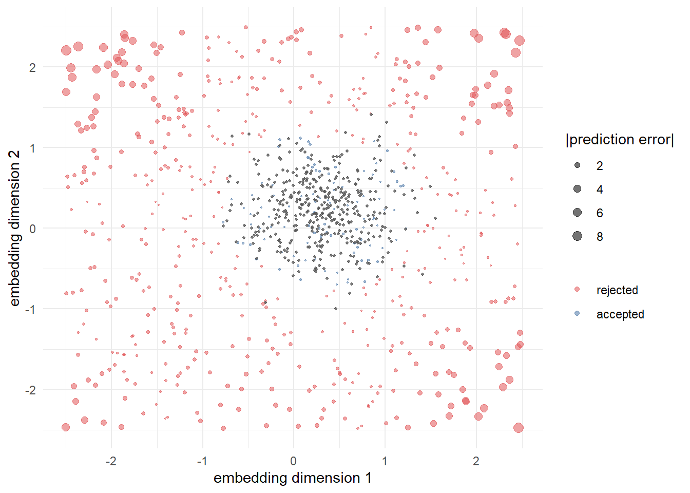
The simulation reproduces the framework’s central claim in the cheapest possible setting: error inside the support is small and roughly homoskedastic, while error outside it is several times larger and grows with distance, even though the fitted model reports no distress in either region. Figure 47.3 makes the geography visible. The managerial reading is that a content-scoring model should return one of two answers—a prediction, or a referral to experimentation—and that the boundary between them is an estimable quantity rather than a matter of taste.
Two caveats travel with this class of method. The support screen protects against extrapolation in the representation, not against a change in the world: a surface fit on last year’s campaigns can be well-supported and still stale if seasonality, competition, or the audience has moved. And embedding-space proximity is a proxy for “similar treatment,” so the screen inherits whatever the embedding model does and does not encode—two subject lines with identical embeddings but different offer terms are not interchangeable treatments. Section 47.9 develops the general version of this warning; Chapter 69 places the framework in the wider generative-AI stack.
47.7.1 Text as Treatment Without an Experiment: Does Puffery Sell?
The causal-prediction framework above assumes the firm can eventually run an experiment. Much marketing text cannot be randomized: a researcher who wants to know whether vague praise in a product description moves demand has only the descriptions that sellers chose to write. Thomas (2026) takes on that problem for puffery, the legal term for exaggerated, unverifiable praise (“luxurious”, “cozy”, “beautiful”). U.S. advertising law tolerates puffery on the premise that consumers discount it, so it cannot mislead. The paper’s own review of the literature finds 13 lab studies of puffery since 1977 and none that observes field purchases. The data are monthly InsideAirbnb scrapes from 2015 to 2019 in 27 cities: 219,335 distinct property descriptions, with nightly calendars that show when each future night was booked. The paper is worth studying for its design as much as for its answer, because nearly every step is a reusable move for anyone who treats observational text as a treatment.
Operationalizing a legal construct with an LLM. Puffery is defined by courts, not by linguists: a claim is puffery when it is too general or subjective to be proven true or false. The paper turns that legal test into a measurement instrument in two steps. First, an LLM (ChatGPT-4o) decomposes each description into its individual claims. Second, it rates each claim on the likelihood, from 0 to 1, that a court would consider it puffery. The ratings are not used as a continuous score. Their histogram is multimodal, and the modes define the categories: objective claims rated 0, weakly subjective claims rated about 0.1 to 0.3 (“near downtown”, “ocean view”), and puffery rated about 0.7 to 0.9. Letting the data’s own gaps set the cutoffs, rather than choosing cutoffs that maximize a booking effect, keeps the outcome out of the measurement. The same logic explains the choice of a pre-existing model. Egami et al. (2022) show that when a text measure is discovered on the same data used to estimate its effect, the discovery step overfits and the resulting inference is invalid; their remedy is a train/test split. A model that was fixed before it saw these listings or their bookings meets the same requirement without spending half the sample. The paper also counts features that need no model: exclamation points, words in all caps, emojis, and stop words. The stop words matter most for identification, as shown below.
The validation follows the discipline of Section 47.5.2, adapted to a construct with no human-labeled corpus of Airbnb text behind it. The LLM’s ratings are checked against claims from legal cases, where courts have already ruled. The main estimate is re-run under alternative cutoffs, under a continuous subjectivity score, and under a transparent bag-of-words measure built from the subjectivity lexicon of Wilson, Wiebe, and Hoffmann (2005) (Section 47.4.1). Agreement across instruments whose errors come from different places is the argument that the category measures puffery and not an artifact of one prompt.
The design. Identification comes from within-listing change. The sample is restricted to description edits that left the photos unchanged: 118,646 changes on 97,185 properties, each new description in place for at least 20 days (90 days in a robustness check). Edits that mention events such as Christmas, or the word “renovated”, are dropped because they signal a change in the product rather than in how it is described. The outcome is not monthly bookings but a booking hazard, estimated as a linear probability model:
\[ y_{idk} = h_{ipk} + g(X_{idk}) + \theta_\tau + \beta' w_{it} + \varepsilon_{idk}, \tag{47.10}\]
where \(y_{idk}\) indicates that night \(d\) of property \(i\) is booked during 30-day lead period \(k\) (six periods cover the 180 days before the stay), \(w_{it}\) counts each claim type in the description shown at scrape date \(t\), and \(h_{ipk}\) are fixed effects for each combination of property, photo set, and lead period (633,920 of them). The hazard framing is what makes the design work. A single description is shown to shoppers for many different future nights at once, and from the point of view of any one stay date, whether the new description arrived early or late in its booking window is close to arbitrary. Each description change is therefore evaluated against many stay dates, which is far more informative than relating a change to aggregate monthly bookings, the outcome used by earlier Airbnb demand work such as Zhang et al. (2022). The regression has 167,637,110 night-by-period observations, with standard errors clustered on the 219,335 descriptions.
Everything else on the page that a host might change at the same time enters through \(g(X_{idk})\): 466 low-dimensional variables, a 384-dimensional text embedding (e5-small) of the rest of the listing page (Section 47.2.4), the number of competitors within half a mile, and a local price index fit with LightGBM. Because \(g\) is high-dimensional, it is estimated by cross-fitting in the style of double machine learning (Chernozhukov et al. 2018): predictions for each observation come from a model fit on other folds, and the adjustment is estimated once and then reused across every specification, which keeps a regression of this size tractable. A fully nonparametric LightGBM version of \(g\) serves as a robustness check.
The update reward. The single most instructive result is a confound that no amount of text control could have caught. In the month of any page update, including new photos, a new host blurb, or a changed amenity list, the booking hazard jumps. The likely cause is the platform’s ranking algorithm rewarding fresh listings (blocked calendar dates may also play a part). Since every description change is also a page update, a within-listing comparison credits that bump to whatever words the host happened to write. The fix is \(\theta_\tau\), fixed effects for months relative to the latest update of any kind, and Table 47.3 shows what it does. The stop words are the giveaway. They carry no meaning a shopper could respond to, yet before \(\theta_\tau\) is added they appear to raise bookings. Once it is added they fall to zero, as a placebo should, and the puffery and objective-claim estimates drop by roughly half or more.
| Feature (one extra) | (1) Property FE | (4) + \(g(X)\) | (6) + months-since-update FE |
|---|---|---|---|
| Puffery claim | 1.88 | 1.28 | 0.65 (0.18) |
| Weakly subjective claim | 2.18 | 1.78 | 1.00 (0.16) |
| Objective claim | 1.87 | 1.42 | 0.52 (0.14) |
| Stop word (placebo) | 0.89 | 0.47 | 0.13 (0.23) |
| Exclamation point | 1.32 | 1.14 | 1.02 (0.41) |
The mechanism is easy to reproduce. In the simulation below, hosts who rewrite a description tend to add claims and words, and the platform rewards any update for a couple of months. Puffery has a true effect of 0.30 and stop words have none.
Code
set.seed(2026)
n <- 4000; n_mon <- 36                       # listings x months
# --- Page updates: ~10% of listing-months; 60% of updates rewrite the text ------
U  <- matrix(runif(n * n_mon) < 0.10, n, n_mon); U[, 1] <- FALSE
Rw <- U & matrix(runif(n * n_mon) < 0.60, n, n_mon)
# Hosts who rewrite tend to ADD claims and words (net drift is positive)
dp <- Rw * matrix(sample(c(-1, 0, 1, 2), n * n_mon, TRUE), n, n_mon)
ds <- Rw * matrix(sample(-2:4,          n * n_mon, TRUE), n, n_mon)
puff <- rpois(n, 3)  + t(apply(dp, 1, cumsum))
stopw <- rpois(n, 20) + t(apply(ds, 1, cumsum))
# Months since the last update of ANY kind (photos too), capped at 6; 99 = none yet
since <- matrix(99L, n, n_mon); last <- rep(NA_integer_, n)
for (m in 1:n_mon) {
  last[U[, m]] <- m
  since[, m] <- ifelse(is.na(last), 99L, pmin(m - last, 6L))
}
# --- Bookings: puffery truly worth 0.30, stop words worth 0, and every update ---
#     earns a transient "update reward" from the platform's ranking
reward <- ifelse(since == 0, 4, ifelse(since == 1, 2, ifelse(since == 2, 1, 0)))
y <- rnorm(n, 0, 2) + 0.30 * puff + 0 * stopw + reward +
  matrix(rnorm(n * n_mon, 0, 1.5), n, n_mon)
# --- Within-listing estimates by demeaning (Frisch-Waugh-Lovell) ----------------
dm <- function(M) as.vector(M - rowMeans(M))           # listing x month matrix
S  <- sapply(0:6, function(k) dm((since == k) * 1))    # 99 (no update yet) = base
est <- function(fit) {                                 # naive (unclustered) SEs
  co <- summary(fit)$coefficients[1:2, 1:2]
  sprintf("%.3f (%.3f)", co[, 1], co[, 2])
}
out <- rbind(est(lm(dm(y) ~ dm(puff) + dm(stopw) - 1)),
             est(lm(dm(y) ~ dm(puff) + dm(stopw) + S - 1)),
             c("0.300", "0.000"))
dimnames(out) <- list(c("Listing FE only", "+ months-since-update FE", "Truth"),
                      c("Puffery claim", "Stop word (placebo)"))
noquote(out)
#>                          Puffery claim Stop word (placebo)
#> Listing FE only          0.385 (0.007) 0.068 (0.004)
#> + months-since-update FE 0.293 (0.005) -0.002 (0.003)
#> Truth                    0.300         0.000
With listing fixed effects alone, puffery is overstated by about 28% and the stop words show a precisely estimated “effect” that cannot be real. Adding fixed effects for months since the last update recovers both truths. The general lesson is that on a platform, the act of editing is itself a treatment. Any study that relates seller-written content to demand through within-listing changes needs a placebo feature that should do nothing, and a control for the editing event itself.
What survives. In the preferred specification, one more puffery claim adds 0.65 booked days per year (95% CI 0.29 to 1.00), about 0.22% over a baseline booking rate of 80%. That is statistically indistinguishable from an objective claim (0.52; \(p = .57\) for the difference). Consumers do not discount puffery to zero, which is the premise of the law, but they do not reward it more than plain facts either. The best-performing category is the weakly subjective claim (1.00, CI 0.68 to 1.32), which beats objective claims (\(p = .019\)) and, less firmly, puffery (\(p = .100\)). Its point estimate is about 55% larger than puffery’s, with a wide interval (−7.9% to 228%). An exclamation point adds 1.02 days (CI 0.22 to 1.83), while all caps and emojis are not significant. Moving from a description at the 25th percentile to one at the 75th adds about 1.35 booked days and $143 in revenue per year. The puffery estimate holds at a cutoff of 0.3 (0.65) and 0.8 (0.55), under the continuous subjectivity score (0.66), and in weaker form under the bag-of-words lexicon (0.40, \(p = .083\)). At the strictest cutoff of 0.9, it vanishes (0.05, SE 0.33), so the most extreme superlatives may do nothing at all. Controlling for sentiment (with the sentimentr lexicon) changes little. Because several claim types change at once, the two-way fixed-effects estimates may be contaminated by heterogeneous effects across treatments (Section 44.1.6). The multi-treatment check of Chaisemartin and D’Haultfœuille (2023) was run, but it is too imprecise to be conclusive either way.
The paper then asks whether puffery leaves guests feeling misled, which is the harm the law’s premise assumes away. It does not appear to. Measured in thousandths of a standard deviation, the effect of a puffery claim on the month-to-month change in a listing’s running average rating is −1.07 (SE 13.11), which rules out effects outside roughly −0.027 to 0.025 SD. Its effect on review sentiment is 7.92 (SE 6.34), with an interval of about −0.005 to 0.020 SD. The all-caps effect is the exception. It lowers ratings (−77.10, SE 34.18, \(p = .024\)) and is associated with lower trust, while objective claims carry a small positive coefficient on ratings (26.32, \(p = .011\)). The paper is explicit about what this cannot show. A booking effect could come from persuasion, where the words change a given shopper’s choice, or from selection, where the words attract shoppers already inclined to like the place. Observational booking data cannot separate the two. A null average effect on satisfaction can also hide offsetting effects across guests.
Three moves transfer directly. A construct defined by an outside authority, such as a court, a regulator, or a professional code, can be measured by asking an LLM to apply that authority’s test claim by claim, provided the cutoffs come from the rating distribution and the model was not tuned on the outcome data. A placebo text feature, like stop words here, is a cheap and sharp falsification test for any within-unit text design. And on a platform, the timing of edits needs its own fixed effects, because the algorithm may be reacting to the edit rather than to what it says. Section 14.3.8 takes up what the finding means for advertising regulation.
47.8 Marketing Applications
The methods above are general; their value is in what they let a marketer measure. Three settings dominate.
Online reviews are the most-mined consumer text, because they pair language with a star rating and often with sales. Review volume and valence track product quality and demand and move firm value, with negative content the most diagnostic (Tirunillai and Tellis 2012; Chevalier and Goolsbee 2003; Godes and Mayzlin 2004). Aspect-based sentiment turns the review corpus into an attribute-level scorecard that tells the firm which feature to fix (Büschken and Allenby 2016), and topic models recover the dimensions of brand perception consumers actually discuss (Tirunillai and Tellis 2014). Reviews also raise their own measurement hazards: figurative language biases naive sentiment (Chapter 48), and the threat of fake reviews makes the classification machinery of Section 47.5 a quality- control necessity rather than an academic exercise.
Social media supplies a continuous, unsolicited signal of brand health that firms mine for “social listening” (Schweidel and Moe 2014). The text is short, noisy, and laden with slang, sarcasm, and emoji, which strains lexicon methods and rewards context-aware representations. The constructs of interest go beyond valence to emotion and stance—how aroused, how powerful, how aligned the writer is toward the brand (Hartmann et al. 2021)—and to network-mediated diffusion, where what and how something is said shapes whether it spreads (Chapter 31; Packard, Gershoff, and Wooten (2016)). Social text also feeds back into measurement of constructs treated elsewhere: blog and post text predict and explain marketing outcomes (Gopinath, Chintagunta, and Venkataraman 2013; Gopinath, Thomas, and Krishnamurthi 2014), and user-generated images extend text measurement into the visual channel (L. Liu, Dzyabura, and Mizik 2020).
Calls and conversations—sales calls, service interactions, support chats—are the frontier, because they are long, dyadic, and rich in the dynamics of persuasion and emotion that static reviews lack. Transcribed and analyzed at scale, they let a firm measure how a frontline agent’s language drives outcomes, where in a conversation sentiment turns, and which conversational moves resolve a complaint—linking directly to the frontline-service and salesperson-value constructs of Chapter 22 and Chapter 15. This is the natural home of LLM extraction (Section 47.6): a transcript is exactly the kind of long, unstructured document from which a prompted model can pull a structured record—intent, objections raised, resolution, sentiment trajectory—that no fixed lexicon or bag-of-words could recover.
Cutting across all three settings is a use of text that deserves separating out: the text measure as a dependent variable in a causal design. When Borwankar et al. (2026) ask what happened to Stack Overflow after it banned ChatGPT-generated content, the outcomes are NLP-derived properties of the posts themselves—length, linguistic complexity, positivity—differenced against a control subreddit (Section 70.6). The design is standard; what is not standard is that the outcome is estimated rather than observed, and that changes the threat model. A generated outcome inherits every bias of the instrument that produced it, and the bias only needs to move with the treatment timing to masquerade as an effect: a lexicon that scores newer slang differently, a hosted classifier silently revised mid-panel, a tokenizer that handles code blocks differently as posts get longer. The discipline is to freeze the measurement pipeline over the full study window, version and log it, and validate it on a hand-coded sample drawn from both the pre and post periods—so that any drift in the instrument is measured rather than absorbed into the treatment effect.
The outcome can also be defined relative to another text. Wang et al. (2026) ask what customers write after a retailer places an AI-generated summary above its reviews (Section 13.5.1). Their content result is stated against the summary. After the summary appears, reviews discuss fewer of the product attributes it already covers and more of the attributes it omits. When they take up a covered attribute, they elaborate on it rather than restate the summary. That is a three-part coding scheme built on the aspect machinery of Section 47.4.6, and each part needs its own instrument. Coverage needs one attribute vocabulary applied identically to the summary and to every review, whether a topic model, a dictionary, or an LLM extractor (Section 47.6). An attribute counts as covered only if the same extractor finds it in both texts. Elaboration versus restatement is a similarity question about the sentences that mention a covered attribute: does the review paraphrase the summary’s sentence, or add a reason, a use case, or a qualification?
The authors’ online appendix documents their pipeline, and it is a good template (Wang et al. 2026, Online Appendices B and O). On the summary side no extraction is needed, because Amazon lists the summary’s attribute keywords under the paragraph and tags each one as positive or negative. On the review side, GPT-4.1 at temperature zero reads one review at a time and returns the attributes it explicitly discusses. The prompt fixes the level of detail with examples (“lasts all day” → “Battery life”, “does not smudge” → “Smudge resistance”) and excludes bare opinions, brands, and delivery complaints. A second LLM pass merges surface variants (“battery”, “how long the charge lasts”) into canonical labels. A review attribute counts as covered when its canonical label matches a summary keyword or one of that keyword’s top-five WordNet synonyms. Elaboration has two measures: the character length of review sentences that mention a covered attribute, and their semantic similarity to the summary’s sentence on the same attribute. Agreement with the summary compares a RoBERTa sentiment classifier’s reading of each attribute sentence with the summary’s tag. For validation, two research assistants hand-coded 200 random reviews. They agreed with each other at Cohen’s \(\kappa = .90\), and the LLM agreed with their consensus at \(\kappa = .86\). Read the raw agreement rates (99.75% and 99.70%) with care. Almost every review-by-attribute cell is a “no”, so percent agreement is close to 100% even for a weak coder. Kappa is the number that carries information here.
A reference text brings hazards that a stand-alone outcome does not. The pipeline above handles some of them and leaves others open.
- A before-and-after comparison needs a counterfactual summary. “Fewer covered attributes after the summary” requires some definition of “covered” for reviews written before any summary existed. One option is to apply the attribute set of the first summary to the pre-period reviews. The authors take this route when they ask which pre-rollout reviews the summary reflects.
- The summary is a moving target. Platforms regenerate summaries as reviews arrive. Coding against the current summary can therefore misclassify the very reviews that changed it: an attribute a reviewer introduced is later absorbed into the summary and then counted as covered. Coverage has to be fixed by the version the reviewer could have seen, which means archiving timestamped snapshots of the summary alongside the reviews. The authors observe that Amazon’s summaries typically update within a week of new reviews, and they code against the updated text. In a weekly panel, that leaves a misclassification window of up to a week.
- The extractor’s recall differs by genre. Fluent, model-written summary prose and terse customer reviews are different genres, and an extractor that finds attributes more reliably in one than in the other shifts the covered/uncovered split mechanically. Validate it on a hand-coded sample of each genre, in the spirit of the pre- and post-period validation above. Using the platform’s own keyword list removes the extractor from the summary side. The risk then moves to vocabulary matching: an LLM label that names the same concept as Amazon’s keyword but is not among its WordNet synonyms counts as uncovered. A constant mismatch rate inflates the uncovered counts but cancels in a before-and-after comparison. It biases that comparison only if the mismatch rate changes once the summary appears. Post-period reviews that borrow the summary’s wording would match more easily, which works against the paper’s finding rather than for it. Spot-check matched and unmatched pairs by hand in both periods.
- Normalization depends on the batch. The list of attribute expressions was too long for one prompt, so it was normalized in batches of 300, followed by a consolidation pass. Batching can give the same concept different labels in different batches. Any residual split inflates attribute counts. Report how many labels the consolidation pass merged, and check that coverage results survive a different batch order.
A second cross-cutting use runs the other way, treating the black-box representation as a yardstick for theory rather than as a substitute for it. Aka and McCoy (2026) predict the memorability of brand slogans—separately for recognition and for cued brand recall—from two competing feature sets: the memorability factors a systematic review extracts from the published literature, operationalized with NLP and human ratings, and raw text embeddings of the slogans themselves. The comparison is the design. Whatever accuracy the embeddings buy beyond the literature-derived factors estimates how much of the phenomenon the accumulated theory has failed to name, converting an uninterpretable representation into a measurement of a literature’s incompleteness. The same audit is available anywhere a research stream has produced a list of proposed textual drivers—ad copy, review helpfulness, email subject lines, headline virality—and never established that the list is exhaustive. Two conditions make it credible: the embedding and the theory-derived features must be evaluated on the same held-out data with the same target, and the gap must be interpreted as an upper bound on what is missing rather than as a discovery, since an embedding that outperforms will not say what it knows. Naming the residual is a separate act of theorizing, and one this design sets up rather than performs.
47.8.1 Auditing a Literature: The Slogan Case Worked
The design is worth running rather than only describing, and Aka and McCoy (2026) make that possible: their replication materials at github.com/adaaka/SloganMemorability post the feature matrix for all 929 slogans—the 25 literature-derived factors, the binomial recognition and cued-recall counts, and 1,536-dimensional embeddings of both the slogan and its brand—alongside the fitted models. Refitting the comparison as ridge-regularized binomial models under ten-fold cross-validation reproduces the design on its own data and returns something a one-line summary of it hides: the audit delivers a different verdict for each outcome.
Code
# Out-of-sample R^2 (squared correlation between predicted and observed rates)
# from a ridge-regularized binomial refit of the posted Aka-McCoy data:
# 929 slogans, 10-fold cross-validation, glmnet with alpha = 0.
cv <- data.frame(
  feature_set = c("Theory factors (25)", "Slogan embedding (1536)",
                  "Slogan + brand embedding (3072)", "Theory + slogan embedding"),
  recognition = c(0.464, 0.499, 0.432, 0.540),
  recall      = c(0.290, 0.148, 0.298, 0.224)
)
print(cv, row.names = FALSE)
#>                      feature_set recognition recall
#>              Theory factors (25)       0.464  0.290
#>          Slogan embedding (1536)       0.499  0.148
#>  Slogan + brand embedding (3072)       0.432  0.298
#>        Theory + slogan embedding       0.540  0.224

# The audit quantity: what does the black box buy beyond the named literature?
emb <- cv$feature_set == "Slogan embedding (1536)"
thy <- cv$feature_set == "Theory factors (25)"
cat(sprintf("\nEmbedding margin over theory-derived factors:\n  recognition %+.3f\n  recall      %+.3f\n",
            cv$recognition[emb] - cv$recognition[thy],
            cv$recall[emb]      - cv$recall[thy]))
#>
#> Embedding margin over theory-derived factors:
#>   recognition +0.035
#>   recall      -0.142
Read the recognition column first, because it is the case the design was built for. The slogan embedding beats the literature’s own factors by \(0.035\)—a real margin, and a modest one. Something about what makes a slogan feel previously seen is carried in the text and not named by the published drivers, but it is a residual rather than a reproach; the factors recover most of what the embedding recovers. That the two feature sets combined outperform either alone (\(0.540\)) settles the more useful question: they are not redundant, so the unnamed component is genuinely additional rather than a re-encoding of the named one.
The recall column inverts the result. Here the theory-derived factors (\(0.290\)) beat the slogan embedding (\(0.148\)) by a wide margin, and the audit’s usual reading—that a literature has failed to name something—is simply wrong. The third row says why: adding the brand’s embedding to the slogan’s lifts recall to \(0.298\), recovering the gap almost exactly. Cued brand recall is a property of the slogan–brand relation, not of the slogan’s text, and slogan text alone cannot encode it; the theory-derived set has it all along through rated brand fit. The general lesson is a constraint on the method: an embedding audit interrogates only the representation it is handed, so a null or negative margin is evidence about that representation’s coverage before it is evidence about the theory’s.
The fourth row carries the estimation caveat. Stacking the 25 factors with the 1,536 embedding dimensions lowers recall accuracy to \(0.224\), below the factors alone, because a single ridge penalty applied across heterogeneous blocks shrinks 25 informative columns toward the scale appropriate for 1,536 weakly informative ones. That is an artifact of the estimator, not a finding about the features—the fix is block-specific penalties (group ridge, or a two-stage fit)—and it is the reason an audit of this kind has to report the comparison it actually ran rather than an abstract contest between “theory” and “embeddings.”
The table is reproducible end to end from the posted files. The script below is the one that produced it; it is not executed when the book is rendered because it downloads a 39 MB feature matrix and refits eight penalized models, but it runs unmodified.
Code
# Reproduces the table above from the Aka-McCoy replication data.
library(glmnet)
base <- "https://raw.githubusercontent.com/adaaka/SloganMemorability/main/dataset/"
d  <- read.csv(paste0(base, "final_dataset_imputed_z_and_embeddings.csv"), check.names = FALSE)
l1 <- read.csv(paste0(base, "level1_mean_z.csv"), check.names = FALSE)

X_fac <- as.matrix(l1[, !(names(l1) %in% c("", "X"))])          # 25 factors
X_sl  <- as.matrix(d[, grep("^ada_embedding_no_", names(d))])   # slogan, 1536 dims
X_br  <- as.matrix(d[, grep("^brand_embeddings_", names(d))])   # brand,  1536 dims

# Binomial outcomes: successes and failures per slogan.
Y <- list(recognition = cbind(d$miss_count,           d$hit_count),
          recall      = cbind(d$sum_incorrect_recall, d$sum_correct_recall))

# Out-of-sample R^2 under 10-fold CV, ridge (alpha = 0) with an inner CV for lambda.
cv_r2 <- function(X, y, nfold = 10, seed = 1) {
  set.seed(seed)
  fold <- sample(rep(1:nfold, length.out = nrow(X)))
  p <- rep(NA_real_, nrow(X))
  for (k in 1:nfold) {
    tr <- fold != k
    fit <- cv.glmnet(X[tr, , drop = FALSE], y[tr, ], family = "binomial",
                     alpha = 0, nfolds = 5)
    p[!tr] <- predict(fit, newx = X[!tr, , drop = FALSE],
                      s = "lambda.min", type = "response")
  }
  cor(p, y[, 2] / rowSums(y))^2
}

sets <- list("Theory factors (25)"             = X_fac,
             "Slogan embedding (1536)"         = X_sl,
             "Slogan + brand embedding (3072)" = cbind(X_sl, X_br),
             "Theory + slogan embedding"       = cbind(X_fac, X_sl))
sapply(Y, function(y) sapply(sets, cv_r2, y = y))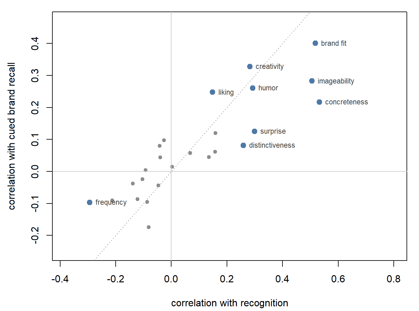
Figure 47.4 makes the split visible in the factors themselves. The drivers that matter for both outcomes are relational and imagistic—rated brand fit (\(r = 0.52\) with recognition, \(0.40\) with recall), concreteness (\(0.53\), \(0.22\)), imageability (\(0.51\), \(0.28\))—while the devices a copywriter reaches for first sit near the origin: alliteration (\(0.14\), \(0.05\)), wordplay (\(0.16\), \(0.06\)), metaphor (\(0.00\), \(0.02\)), hyperbole (\(0.07\), \(0.06\)). Word frequency is the one clearly negative driver for recognition (\(-0.29\)), which is what a recognition test should do—common vocabulary is precisely what a memory probe cannot discriminate. Points fall well off the diagonal, and the two outcomes correlate only \(0.46\) across slogans, which is the empirical warrant for the paper’s decision to model them separately rather than to average them into one memorability score.
47.9 Pitfalls and Identification
Text-as-data inherits every threat to validity that afflicts measurement, plus several of its own. Naming them is the precondition for credible inference.
The deepest is that the representation is an identifying assumption. A bag-of-words cannot represent negation or sarcasm, so any inference from it about valence is conditional on those phenomena being rare or randomly distributed—an assumption that is often false and rarely tested (Chapter 48). The choice of representation is therefore not a tuning detail but a substantive claim about what the text means.
A second hazard is selection in who writes. The corpus is generated by people who chose to review, post, or call, and that selection is correlated with the outcome: reviewers are disproportionately the delighted and the furious, producing the well-known J-shaped ratings distribution, and social-media posters are not a random sample of customers. Text measured on a selected sample estimates the sentiment of writers, not of customers, and the gap is a bias, not noise. Methods that debias the poster population are the appropriate response, not a larger but equally selected corpus.
A third is endogeneity in downstream regressions. When a text-derived measure—topic share, sentiment, an LLM-extracted field—is used as a regressor explaining sales or firm value, it is a generated regressor measured with error and often correlated with omitted drivers. Plugging \(\hat{s}_i\) into a regression as if it were observed understates standard errors and can bias coefficients; the measurement model and the outcome model should be treated as one system, and the error in the text measure propagated. The marketing-finance and metrics chapters (Chapter 26, Chapter 32) develop the downstream inference that text measures feed.
Finally, validation is not optional and is not a formality. Every text measure— lexicon score, topic label, classifier output, LLM extraction—is a claim about an unobserved construct and must be validated against human-coded ground truth on a sample, with an explicit reliability statistic, before it enters an analysis (Section 48.5). A pipeline that reports its accuracy on the data it was tuned on, or that never compares its output to human judgment at all, has produced numbers, not measurements. The discipline that distinguishes text-as-data from text mining is precisely this insistence that a column of model output earn the status of data.
47.10 Key Takeaways
- An embedding can audit a literature, not just beat it. Scoring theory-derived features against raw embeddings on the same held-out target turns the accuracy gap into an estimate of how much of a phenomenon the published drivers fail to name—demonstrated for slogan memorability across recognition and cued brand recall (Aka and McCoy 2026). The gap is an upper bound on what is missing, not a discovery: the embedding will not say what it knows. The verdict is also outcome-specific. Refit on the posted data (Section 47.8.1), embeddings beat the named factors on recognition by \(0.035\) but lose to them on cued brand recall by \(0.142\), because recall depends on the slogan–brand relation that slogan text alone cannot encode. An audit interrogates only the representation it is handed.
- Representation is the first and most consequential choice. Bag-of-words and TF-IDF are transparent but order- and context-blind (Equation 47.1, Equation 47.2); embeddings capture context at the cost of interpretability (Section 47.2.4). Match the representation to the construct, not to fashion.
- Topic models discover structure but do not name it. LDA’s outputs are distributions an analyst must interpret and validate; \(K\) and the priors are researcher choices, not data, and the solution is sensitive to them (Section 47.3.1).
- Sentiment, emotion, and stance are distinct constructs. Lexicons are auditable but cannot represent negation or sarcasm, biasing estimates in a signed way (Section 47.4.1, Chapter 48); decide which construct, at which level, validated how, before scoring.
- A domain dictionary can be grown from seed words with embeddings, but it inherits the corpus’s vocabulary. Culture dictionaries expanded from job postings pick up occupation words (“customer” for quality, “team” for respect), so scores are comparable only within occupation. Within that limit, culture language in job ads predicts worker inflows, offers, and acceptances (Huang et al. 2026; K. Li et al. 2021) (Section 47.4.2).
- Supervised classification lives or dies by honest evaluation. Under class imbalance, report precision, recall, and F1, guard against leakage, and validate out-of-distribution (Section 47.5.2).
- LLMs are powerful, cheap annotators—and unvalidated classifiers until proven otherwise. Hallucination, prompt sensitivity, and contamination make validation more necessary, not less (Section 47.6).
- Selection, generated-regressor error, and validation against ground truth are the identification frontier; text measured on who chose to write estimates writers, not customers (Section 47.9).
Aka, Ada, and John McCoy. 2026. “Predicting the Memorability of Brand Slogans.” Journal of Marketing Research. https://doi.org/10.1177/00222437261481110.
Ananthakrishnan, Uttara M, Naveen Basavaraj, Sabari Rajan Karmegam, Ananya Sen, and Michael D Smith. 2025. “Book Bans in American Libraries: Impact of Politics on Inclusive Content Consumption.” Marketing Science.
Balducci, Bitty, and Detelina Marinova. 2018. “Unstructured Data in Marketing.” Journal of the Academy of Marketing Science 46 (4): 557–90. https://doi.org/10.1007/s11747-018-0581-x.
Berger, Jonah, Ashlee Humphreys, Stephan Ludwig, Wendy W. Moe, Oded Netzer, and David A. Schweidel. 2020. “Uniting the Tribes: Using Text for Marketing Insight.” Journal of Marketing 84 (1): 1–25. https://doi.org/10.1177/0022242919873106.
Blei, David M., and Michael I. Jordan. 2003. “Modeling Annotated Data.” In Proceedings of the 26th Annual International ACM SIGIR Conference on Research and Development in Information Retrieval, 127–34. https://doi.org/10.1145/860435.860460.
Blei, David M., Andrew Y. Ng, and Michael I. Jordan. 2002. “Latent Dirichlet Allocation.” In Advances in Neural Information Processing Systems 14 (NIPS 2001), 601–8. MIT Press. https://doi.org/10.7551/mitpress/1120.003.0082.
Borwankar, Sameer, Warut Khern-am-nuai, Anastasiya Ghosh, and Karthik Kannan. 2026. “Unraveling the Impact: An Empirical Investigation of ChatGPT’s Exclusion from Stack Overflow.” Information Systems Research. https://doi.org/10.1287/isre.2024.1235.
Boustanifar, Hamid, and Arnt Verriest. 2026. “Intangible Liabilities.” Management Science 72 (11): 9990–10019. https://doi.org/10.1287/mnsc.2023.03619.
Büschken, Joachim, and Greg M Allenby. 2016. “Sentence-Based Text Analysis for Customer Reviews.” Marketing Science 35 (6): 953–75.
Chaisemartin, Clément de, and Xavier D’Haultfœuille. 2023. “Two-Way Fixed Effects and Differences-in-Differences Estimators with Several Treatments.” Journal of Econometrics 236 (2): 105480. https://doi.org/10.1016/j.jeconom.2023.105480.
Chernozhukov, Victor, Denis Chetverikov, Mert Demirer, Esther Duflo, Christian Hansen, Whitney Newey, and James Robins. 2018. “Double/Debiased Machine Learning for Treatment and Structural Parameters.” The Econometrics Journal 21 (1): C1–68. https://doi.org/10.1111/ectj.12097.
Chevalier, Judith, and Austan Goolsbee. 2003. “Measuring Prices and Price Competition Online: Amazon. Com and BarnesandNoble. Com.” Quantitative Marketing and Economics 1 (2): 203–22.
Devlin, Jacob, Ming-Wei Chang, Kenton Lee, and Kristina Toutanova. 2019. “BERT: Pre-Training of Deep Bidirectional Transformers for Language Understanding.” In Proceedings of the 2019 Conference of the North American Chapter of the Association for Computational Linguistics (NAACL-HLT), 4171–86. https://doi.org/10.18653/v1/n19-1423.
Dieng, Adji B., Francisco J. R. Ruiz, and David M. Blei. 2020. “Topic Modeling in Embedding Spaces.” Transactions of the Association for Computational Linguistics 8: 439–53. https://doi.org/10.1162/tacl_a_00325.
Egami, Naoki, Christian J. Fong, Justin Grimmer, Margaret E. Roberts, and Brandon M. Stewart. 2022. “How to Make Causal Inferences Using Texts.” Science Advances 8 (42): eabg2652. https://doi.org/10.1126/sciadv.abg2652.
Ellickson, Paul B., Wreetabrata Kar, and James C. Reeder. 2023. “Estimating Marketing Component Effects: Double Machine Learning from Targeted Digital Promotions.” Marketing Science 42 (4): 704–28. https://doi.org/10.1287/mksc.2022.1401.
Ellickson, Paul B., Wreetabrata Kar, James C. Reeder, and Guang Zeng. 2026. “Evaluating Novel Unstructured Treatments with Generative AI: A Causal Prediction Framework.” Journal of Marketing Research. https://doi.org/10.1177/00222437261476639.
Gabel, Sebastian, Daniel Guhl, and Daniel Klapper. 2019. “P2V-MAP: Mapping Market Structures for Large Retail Assortments.” Journal of Marketing Research 56 (4): 557–80. https://doi.org/10.1177/0022243719833631.
Gao, Janet, Wenyu Wang, and Xiaoyun Yu. 2024. “Big Fish in Small Ponds: Human Capital Migration and the Rise of Boutique Banks.” Management Science.
Godes, David, and Dina Mayzlin. 2004. “Using Online Conversations to Study Word-of-Mouth Communication.” Marketing Science 23 (4): 545–60. https://doi.org/10.1287/mksc.1040.0071.
Gopinath, Shyam, Pradeep K Chintagunta, and Sriram Venkataraman. 2013. “Blogs, Advertising, and Local-Market Movie Box Office Performance.” Management Science 59 (12): 2635–54.
Gopinath, Shyam, Jacquelyn S Thomas, and Lakshman Krishnamurthi. 2014. “Investigating the Relationship Between the Content of Online Word of Mouth, Advertising, and Brand Performance.” Marketing Science 33 (2): 241–58.
Guiso, Luigi, Paola Sapienza, and Luigi Zingales. 2015. “The Value of Corporate Culture.” Journal of Financial Economics 117 (1): 60–76. https://doi.org/10.1016/j.jfineco.2014.05.010.
Hartmann, Jochen, Mark Heitmann, Christina Schamp, and Oded Netzer. 2021. “The Power of Brand Selfies.” Journal of Marketing Research 58 (6): 1159–77.
Hartmann, Jochen, Mark Heitmann, Christian Siebert, and Christina Schamp. 2023. “More Than a Feeling: Accuracy and Application of Sentiment Analysis.” International Journal of Research in Marketing 40 (1): 75–87.
Henry, Elaine, and Andrew J. Leone. 2016. “Measuring Qualitative Information in Capital Markets Research: Comparison of Alternative Methodologies to Measure Disclosure Tone.” The Accounting Review 91 (1): 153–78. https://doi.org/10.2308/accr-51161.
Huang, Allen H., Joseph Pacelli, Terrence Tianshuo Shi, and Yuan Zou. 2026. “Communicating Corporate Culture in Labor Markets: Evidence from Job Postings.” Management Science. https://doi.org/10.1287/mnsc.2024.07272.
Humphreys, Ashlee, and Rebecca Jen-Hui Wang. 2018. “Automated Text Analysis for Consumer Research.” Journal of Consumer Research 44 (6): 1274–1306. https://doi.org/10.1093/jcr/ucx104.
Kogan, Shimon, Dimitry Levin, Bryan R. Routledge, Jacob S. Sagi, and Noah A. Smith. 2009. “Predicting Risk from Financial Reports with Regression.” In Proceedings of Human Language Technologies: The 2009 Annual Conference of the North American Chapter of the Association for Computational Linguistics. Association for Computational Linguistics. https://doi.org/10.3115/1620754.1620794.
Lee, Jungho. 2026. “Start-up Firms and Corporate Culture: Evidence from Advertised Corporate Culture.” Management Science 72 (10): 9237–53. https://doi.org/10.1287/mnsc.2023.00254.
Li, Jiazheng, Linyi Yang, Barry Smyth, and Ruihai Dong. 2020. “MAEC: A Multimodal Aligned Earnings Conference Call Dataset for Financial Risk Prediction.” In Proceedings of the 29th ACM International Conference on Information & Knowledge Management, 3063–70. ACM. https://doi.org/10.1145/3340531.3412879.
Li, Kai, Feng Mai, Rui Shen, and Xinyan Yan. 2021. “Measuring Corporate Culture Using Machine Learning.” The Review of Financial Studies 34 (7): 3265–315. https://doi.org/10.1093/rfs/hhaa079.
Liu, Baixiao, and Linlin Ma. 2026. “Media Sentiment on Foreign Countries and International Asset Allocation.” Management Science. https://doi.org/10.1287/mnsc.2024.05504.
Liu, Liu, Daria Dzyabura, and Natalie Mizik. 2020. “Visual Listening In: Extracting Brand Image Portrayed on Social Media.” Marketing Science 39 (4): 669–86. https://doi.org/10.1287/mksc.2020.1226.
Loughran, Tim, and Bill McDonald. 2011. “When Is a Liability Not a Liability? Textual Analysis, Dictionaries, and 10-Ks.” The Journal of Finance 66 (1): 35–65. https://doi.org/10.1111/j.1540-6261.2010.01625.x.
Melumad, Shiri, and Michel Tuan Pham. 2020. “The Smartphone as a Pacifying Technology.” Edited by Darren W Dahl, Amna Kirmani, and Peter R Darke. Journal of Consumer Research 47 (2): 237–55. https://doi.org/10.1093/jcr/ucaa005.
Netzer, Oded, Ronen Feldman, Jacob Goldenberg, and Moshe Fresko. 2012. “Mine Your Own Business: Market-Structure Surveillance Through Text Mining.” Marketing Science 31 (3): 521–43. https://doi.org/10.1287/mksc.1120.0713.
Netzer, Oded, and V. Srinivasan. 2011. “Adaptive Self-Explication of Multiattribute Preferences.” Journal of Marketing Research 48 (1): 140–56. https://doi.org/10.1509/jmkr.48.1.140.
Nguyen, Dat Quoc, Richard Billingsley, Lan Du, and Mark Johnson. 2015. “Improving Topic Models with Latent Feature Word Representations.” Transactions of the Association for Computational Linguistics 3: 299–313. https://doi.org/10.1162/tacl_a_00140.
Pacelli, Joseph, Tianshuo Shi, and Yuan Zou. 2023. “Communicating Corporate Culture in Labor Markets: Evidence from Job Postings.” Working paper. Harvard Business School. https://www.anderson.ucla.edu/sites/default/files/document/2023-03/Pacelli-Paper.pdf.
Packard, Grant, Andrew D. Gershoff, and David B. Wooten. 2016. “When Boastful Word of Mouth Helps Versus Hurts Social Perceptions and Persuasion.” Journal of Consumer Research 43 (1): 26–43. https://doi.org/10.1093/jcr/ucw009.
Packard, Grant, and David B. Wooten. 2013. “Compensatory Knowledge Signaling in Consumer Word-of-Mouth.” Journal of Consumer Psychology 23 (4): 434–50. https://doi.org/10.1016/j.jcps.2013.05.002.
Pennington, Jeffrey, Richard Socher, and Christopher D. Manning. 2014. “GloVe: Global Vectors for Word Representation.” In Proceedings of the 2014 Conference on Empirical Methods in Natural Language Processing (EMNLP), 1532–43. https://doi.org/10.3115/v1/d14-1162.
Qian, Yang, Hai Che, Yezheng Liu, Yuanchun Jiang, and Jennifer Shang. 2026. “Deriving Competitive Intelligence from Multifaceted User Behavior Data: An Interpretable Machine Learning Framework.” Production and Operations Management 35 (12): 4447–63. https://doi.org/10.1177/10591478261457235.
Ringel, Daniel M., and Bernd Skiera. 2016. “Visualizing Asymmetric Competition Among More Than 1,000 Products Using Big Search Data.” Marketing Science 35 (3): 511–34. https://doi.org/10.1287/mksc.2015.0950.
Sang, Yunxin, and Yang Bao. 2022. “DialogueGAT: A Graph Attention Network for Financial Risk Prediction by Modeling the Dialogues in Earnings Conference Calls.” In Findings of the Association for Computational Linguistics: EMNLP 2022, 1623–33. Association for Computational Linguistics. https://doi.org/10.18653/v1/2022.findings-emnlp.117.
Schweidel, David A, and Wendy W Moe. 2014. “Listening in on Social Media: A Joint Model of Sentiment and Venue Format Choice.” Journal of Marketing Research 51 (4): 387–402.
Shannon, C. E. 1948. “A Mathematical Theory of Communication.” Bell System Technical Journal 27 (3): 379–423. https://doi.org/10.1002/j.1538-7305.1948.tb01338.x.
Thomas, Michael. 2026. “Does Puffery Sell? Evidence from Airbnb.” Journal of Marketing Research 63 (6): 1074–94. https://doi.org/10.1177/00222437261444259.
Tirunillai, Seshadri, and Gerard J. Tellis. 2012. “Does Chatter Really Matter? Dynamics of User-Generated Content and Stock Performance.” Marketing Science 31 (2): 198–215. https://doi.org/10.1287/mksc.1110.0682.
———. 2014. “Mining Marketing Meaning from Online Chatter: Strategic Brand Analysis of Big Data Using Latent Dirichlet Allocation.” Journal of Marketing Research 51 (4): 463–79. https://doi.org/10.1509/jmr.12.0106.
Tran, Chi Phuong. 2023. “Consumer Engagement in the Digital Era.” PhD thesis, University of Oregon. https://hdl.handle.net/1794/29217.
Tran, Chi P., Nooshin L. Warren, and Joshua T. Beck. 2026. “How the #MeToo Movement Has Reshaped Gender Dynamics in the Marketplace: Evidence from the Entertainment Industry.” Journal of Marketing. https://doi.org/10.1177/00222429261464934.
Wang, Qili, Yi Su, Liangfei Qiu, and Runyu Chen. 2026. “Navigating the Sea of Reviews: Unveiling the Effects of Introducing AI-Generated Summaries in e-Commerce.” Information Systems Research. https://doi.org/10.1287/isre.2024.1282.
Weaver, Warren, Claude E Shannon, et al. 1963. The Mathematical Theory of Communication. Vol. 517. University of Illinois Press Champaign, IL.
Wilson, Theresa, Janyce Wiebe, and Paul Hoffmann. 2005. “Recognizing Contextual Polarity in Phrase-Level Sentiment Analysis.” In Proceedings of the Conference on Human Language Technology and Empirical Methods in Natural Language Processing (HLT/EMNLP 2005), 347–54. https://doi.org/10.3115/1220575.1220619.
Yang, Yi, Yixuan Tang, Yangyang Fan, and Kunpeng Zhang. 2026. “Learning from Earnings Calls: Graph-Based Conversational Modeling for Financial Prediction.” Information Systems Research 37 (3): 1681–1705. https://doi.org/10.1287/isre.2023.0519.
Zhang, Shunyuan, Dokyun Lee, Param Vir Singh, and Kannan Srinivasan. 2022. “What Makes a Good Image? Airbnb Demand Analytics Leveraging Interpretable Image Features.” Management Science 68 (8): 5644–66. https://doi.org/10.1287/mnsc.2021.4175.
Cite this section
Nguyen, M. (2026). Text as Data. In Marketing research: A technical and academic treatment. https://mikenguyen13.github.io/marketing_research/49-text-as-data.html
BibTeX
@inbook{Nguyen2026Marketing-49-text-as-data,
  author    = {Nguyen, Mike},
  title     = {Marketing Research: A Technical and Academic Treatment},
  chapter   = {Text as Data},
  year      = {2026},
  url       = {https://mikenguyen13.github.io/marketing_research/49-text-as-data.html}
}
Use this book with your AI assistant
Ask questions about this book in Claude, Cursor, VS Code, or ChatGPT, with answers that cite the section.
https://research-methods-mcp.vercel.app/mcp?src=book-marketing-research

