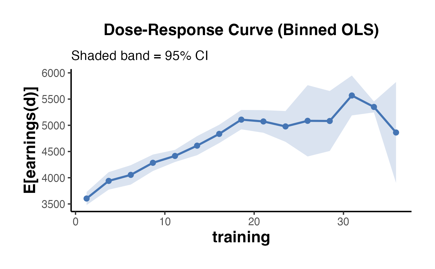
Dose-Response Curve for Continuous Treatment

Estimates the dose-response function for a continuous treatment using one of three methods and plots the resulting curve with a shaded 95% CI ribbon. The IPW approach follows Hirano & Imbens (2004).

Usage

dose_response_curve(
  data,
  outcome,
  treatment,
  covariates = NULL,
  n_bins = 20,
  method = c("ipw", "ols", "gam"),
  plot = TRUE
)

Arguments

data

A data frame.

outcome

Character. Name of the continuous outcome variable.

treatment

Character. Name of the continuous treatment variable.

covariates

Character vector. Names of pre-treatment covariates to adjust for. NULL for unadjusted estimates.

n_bins

Integer. Number of bins for the treatment axis. Default 20.

method

Character. Estimation method: "ipw" (generalised propensity score weighting), "ols" (binned local means), or "gam" (GAM via mgcv, if available). Default "ipw".

plot

Logical. Whether to print and return the plot. Default TRUE.

Value

A named list:

curve_df

Data frame with columns dose_mid, estimate, ci_lo, ci_hi, n (observations in each bin).

plot

A ggplot2 object, or NULL if plot = FALSE.

Details

Dose-Response Curve Estimation for Continuous Treatments

Estimates and visualises the average potential outcome E[Y(d)] as a function of a continuous treatment dose d. Three estimation strategies are available: inverse-probability weighting with a generalised propensity score (IPW), binned OLS, and a generalised additive model (GAM). Returns the estimated curve with 95% confidence intervals and a ggplot2 object.

References

Hirano, K., & Imbens, G. W. (2004). The propensity score with continuous treatments. In A. Gelman & X.-L. Meng (Eds.), Applied Bayesian Modeling and Causal Inference from Incomplete-Data Perspectives. Wiley.

Examples

set.seed(123)
n   <- 600
age <- rnorm(n, 35, 10)
# Continuous dose: hours of training (0-40)
dose <- pmax(0, 10 + 3 * (age - 35) / 10 + rnorm(n, 0, 8))
y    <- 2000 + 80 * dose - 1.5 * dose^2 + 50 * age + rnorm(n, 0, 500)
df   <- data.frame(earnings = y, training = dose, age = age)

result <- dose_response_curve(
  data       = df,
  outcome    = "earnings",
  treatment  = "training",
  covariates = "age",
  n_bins     = 15,
  method     = "ols"
)
result$plot