7. Event Studies (Finance)
Mike Nguyen
2026-03-22
h_event_study.Rmd
library(causalverse)1. Introduction
1.1 What Is a Finance Event Study?
The finance event study is one of the most widely used empirical methods in financial economics. Its purpose is to measure the impact of a specific economic event on the value of a firm by examining abnormal stock returns around the time of that event. The logic is rooted in the efficient markets hypothesis: if markets are informationally efficient, the effect of a new piece of information (an “event”) should be reflected quickly in security prices. By comparing observed returns to a benchmark of “normal” returns, the researcher isolates the abnormal return attributable to the event.
Finance event studies have been applied to an enormous range of corporate and economic events, including:
- Earnings announcements – measuring how the market responds to unexpected earnings surprises.
- Mergers and acquisitions – assessing wealth effects for acquiring and target firm shareholders.
- Dividend announcements – testing dividend signaling hypotheses.
- Stock splits – evaluating the information content of split decisions.
- Regulatory and policy changes – quantifying how new regulations affect firm value.
- CEO turnover – measuring the market’s assessment of leadership changes.
- Credit rating changes – assessing the informational value of ratings.
- Natural disasters and geopolitical shocks – evaluating exposure and market resilience.
The core output of a finance event study is the abnormal return (AR) for individual event dates and the cumulative abnormal return (CAR) aggregated over a short window surrounding the event. These quantities, combined with appropriate statistical tests, allow researchers to draw inferences about whether an event conveyed economically significant new information to the market.
1.2 A Brief History
The finance event study has a long and distinguished lineage:
- Ball and Brown (1968) pioneered the methodology by studying the information content of annual earnings announcements, showing that stock prices adjust to earnings information in advance of the formal announcement date.
- Fama, Fisher, Jensen, and Roll (1969) provided the first rigorous event study of stock splits, establishing many of the methodological conventions still used today. Their paper demonstrated that the event study could isolate the effect of a single event from other concurrent market movements.
- Brown and Warner (1980, 1985) conducted extensive simulation studies evaluating the statistical properties of event study methods, both for monthly and daily data. Their work established the conditions under which standard tests are well-specified and powerful.
- MacKinlay (1997) authored the definitive survey of finance event study methodology, covering estimation procedures, statistical tests, and practical considerations. This paper remains the standard reference.
- Campbell, Lo, and MacKinlay (1997) provided textbook treatment of the methodology in Chapter 4 of The Econometrics of Financial Markets.
- Kothari and Warner (2007) surveyed the evolution of event study methods with particular emphasis on long-horizon studies and their statistical challenges.
1.3 Finance Event Studies vs. Econometric Event Studies
It is essential to distinguish finance event studies from econometric event studies (also called dynamic DID or event-study designs in the causal inference literature). These are fundamentally different methodologies despite sharing the name “event study”:
| Feature | Finance Event Study | Econometric Event Study |
|---|---|---|
| Outcome | Stock returns (or other asset prices) | Any panel outcome (wages, crime, health, etc.) |
| Benchmark | Market model, factor model | Parallel trends (control group) |
| Window | Typically short (days) | Often long (months/years) |
| Unit | Individual security | Treated vs. control units |
| Goal | Measure abnormal return | Estimate dynamic treatment effects |
| Key assumption | Efficient markets | Parallel trends |
| Key references | MacKinlay (1997), Fama et al. (1969) | Sun & Abraham (2021), Callaway & Sant’Anna (2021) |
The econometric event study is covered in other vignettes in this package (see the DID and staggered treatment vignettes). This vignette focuses exclusively on the finance tradition.
2. The Event Study Framework
2.1 Timeline and Windows
A finance event study divides time into three distinct windows relative to the event date :
Estimation window : A period before the event used to estimate the parameters of the normal return model. A common choice is to (i.e., roughly one trading year ending 21 days before the event). The estimation window should be long enough to obtain precise parameter estimates but should not overlap with the event window, so that the event itself does not contaminate the normal return model.
-
Event window : The period surrounding the event date over which abnormal returns are computed. Common choices include:
- : a three-day window capturing the announcement day and one day on either side (to account for after-hours announcements and information leakage).
- : an eleven-day window for events where information may leak or the market may take longer to fully process the news.
- : a twenty-one-day window used for events with greater uncertainty about the precise information release date.
- : a single-day window when the event date is known precisely.
Post-event window : An optional window used in long-run event studies to assess whether the market’s initial reaction is permanent or transient.
The timeline can be visualized as follows:
|<--- Estimation Window --->|  Gap  |<-- Event Window -->|<-- Post-Event -->|
T0                          T1      T1+1    tau=0     T2  T2+1            T3
The gap between the estimation window and the event window (often 10-20 trading days) is a buffer to prevent contamination from pre-event information leakage.
2.2 Normal Return Models
The normal return model specifies the expected return for security at time in the absence of the event. The abnormal return is then the difference between the actual return and this expected return. Several models are commonly used:
2.2.1 Constant Mean Return Model
The simplest model assumes that the expected return for security is constant over time:
The abnormal return is:
where is the sample mean return of security over the estimation window. This model is surprisingly effective in short-window studies because the variance of abnormal returns is dominated by the firm-specific component, not the expected return component (Brown and Warner, 1985).
2.2.2 Market Model
The market model is the workhorse of finance event studies. It assumes a linear relationship between the return on security and the return on the market portfolio:
where is the market return (typically the CRSP value-weighted index or S&P 500), and are firm-specific parameters estimated by OLS over the estimation window, and is the zero-mean disturbance term. The abnormal return is:
The market model generally reduces the variance of abnormal returns relative to the constant mean return model (because it removes the portion of return variation attributable to market-wide movements), thereby increasing the power of statistical tests.
2.2.3 Market-Adjusted Return Model
The market-adjusted return model is a restricted version of the market model with and :
This model requires no estimation window and is useful when the estimation window is contaminated or unavailable. It implicitly assumes that all firms have the same systematic risk exposure.
2.3 Abnormal Returns
Given a normal return model with estimated parameters, the abnormal return for security on event day is:
For the market model, this becomes:
2.4 Cumulative Abnormal Returns (CAR)
To aggregate abnormal returns over the event window , we compute the cumulative abnormal return:
The CAR captures the total abnormal price movement over the event window. In cross-sectional analysis, we compute the average CAR across all event firms:
2.5 Buy-and-Hold Abnormal Returns (BHAR)
For long-horizon event studies, the buy-and-hold abnormal return is preferred over CAR because it better reflects the actual investment experience:
BHAR compounds actual returns and benchmark returns separately, then takes the difference. This avoids the rebalancing bias inherent in CARs over long horizons.
3. Simulated Data
We create a simulated dataset of stock returns for multiple firms, each experiencing an event at a known date. This allows us to demonstrate the methodology with fully reproducible code.
set.seed(42)

# Parameters
n_firms      <- 50       # Number of firms experiencing events
n_days       <- 300      # Total trading days per firm
event_day    <- 200      # Event occurs on day 200 for all firms
est_start    <- 1        # Estimation window start
est_end      <- 170      # Estimation window end
gap          <- 10       # Gap between estimation and event windows
event_start  <- est_end + gap + 1   # Event window start
event_end    <- n_days   # End of sample

# True parameters for the market model
true_alpha <- rnorm(n_firms, mean = 0.0002, sd = 0.0005)
true_beta  <- rnorm(n_firms, mean = 1.0, sd = 0.3)

# Simulate market returns (daily)
market_ret <- rnorm(n_days, mean = 0.0004, sd = 0.012)

# Abnormal return injection: 2% positive abnormal return on event day,
# with small leakage on day -1 and persistence on day +1
true_event_effect <- rep(0, n_days)
true_event_effect[event_day - 1] <- 0.005   # Pre-event leakage
true_event_effect[event_day]     <- 0.020   # Main event effect
true_event_effect[event_day + 1] <- 0.003   # Post-event drift

# Simulate firm returns
sim_data <- do.call(rbind, lapply(1:n_firms, function(i) {
    eps <- rnorm(n_days, mean = 0, sd = 0.02)
    ret <- true_alpha[i] + true_beta[i] * market_ret + eps + true_event_effect
    data.frame(
        firm_id    = i,
        day        = 1:n_days,
        event_time = (1:n_days) - event_day,
        ret        = ret,
        market_ret = market_ret,
        stringsAsFactors = FALSE
    )
}))

# Add firm characteristics for cross-sectional analysis
firm_chars <- data.frame(
    firm_id   = 1:n_firms,
    log_mcap  = rnorm(n_firms, mean = 8, sd = 1.5),     # Log market cap
    leverage  = runif(n_firms, min = 0.1, max = 0.8),    # Debt/assets
    roa       = rnorm(n_firms, mean = 0.05, sd = 0.03),  # Return on assets
    stringsAsFactors = FALSE
)

sim_data <- merge(sim_data, firm_chars, by = "firm_id")

head(sim_data)
#>   firm_id day event_time          ret   market_ret log_mcap  leverage
#> 1       1   1       -199  0.043825782  0.014811585 9.179422 0.3662711
#> 2       1   2       -198 -0.002313518  0.012937013 9.179422 0.3662711
#> 3       1   3       -197 -0.010767304 -0.011638504 9.179422 0.3662711
#> 4       1   4       -196  0.026629494  0.022581783 9.179422 0.3662711
#> 5       1   5       -195 -0.019017030 -0.007601281 9.179422 0.3662711
#> 6       1   6       -194 -0.017262214  0.001666166 9.179422 0.3662711
#>          roa
#> 1 0.05485505
#> 2 0.05485505
#> 3 0.05485505
#> 4 0.05485505
#> 5 0.05485505
#> 6 0.05485505
Let us verify the structure of the simulated data:
cat("Number of firms:", length(unique(sim_data$firm_id)), "\n")
#> Number of firms: 50
cat("Days per firm:", n_days, "\n")
#> Days per firm: 300
cat("Event day:", event_day, "\n")
#> Event day: 200
cat("Estimation window:", est_start, "to", est_end, "\n")
#> Estimation window: 1 to 170
cat("Event window start:", event_start, "\n")
#> Event window start: 181
cat("Total observations:", nrow(sim_data), "\n")
#> Total observations: 15000
4. Market Model Estimation
4.1 OLS Estimation in the Estimation Window
The first step is to estimate the market model parameters for each firm using data from the estimation window only.
# Define estimation window
est_window <- sim_data %>%
    filter(day >= est_start & day <= est_end)

# Estimate market model for each firm using lm()
market_models <- lapply(1:n_firms, function(i) {
    firm_est <- est_window %>% filter(firm_id == i)
    lm(ret ~ market_ret, data = firm_est)
})

# Extract parameters
model_params <- data.frame(
    firm_id = 1:n_firms,
    alpha   = sapply(market_models, function(m) coef(m)[1]),
    beta    = sapply(market_models, function(m) coef(m)[2]),
    sigma   = sapply(market_models, function(m) summary(m)$sigma),
    r_sq    = sapply(market_models, function(m) summary(m)$r.squared)
)

# Summary of estimated parameters
summary(model_params[, c("alpha", "beta", "sigma", "r_sq")])
#>      alpha                 beta            sigma              r_sq
#>  Min.   :-4.062e-03   Min.   :0.2716   Min.   :0.01777   Min.   :0.01831
#>  1st Qu.:-1.130e-03   1st Qu.:0.8498   1st Qu.:0.01920   1st Qu.:0.20161
#>  Median :-1.153e-04   Median :1.0376   Median :0.01999   Median :0.24660
#>  Mean   :-9.098e-05   Mean   :1.0378   Mean   :0.02005   Mean   :0.25850
#>  3rd Qu.: 7.438e-04   3rd Qu.:1.2000   3rd Qu.:0.02093   3rd Qu.:0.32906
#>  Max.   : 3.196e-03   Max.   :1.7322   Max.   :0.02257   Max.   :0.49734
4.2 Estimation Using fixest::feols()
For larger datasets or panel estimation, fixest::feols() provides a fast alternative. Here we estimate the market model with firm fixed effects to demonstrate the syntax:
# Estimate the market model for each firm using fixest
# Split estimation by firm using the split argument
fixest_models <- feols(
    ret ~ market_ret,
    data  = est_window,
    split = ~firm_id
)

# Show results for first firm
summary(fixest_models[[1]])
#> OLS estimation, Dep. Var.: ret
#> Observations: 170
#> Sample (firm_id): 1
#> Standard-errors: IID
#>             Estimate Std. Error  t value   Pr(>|t|)
#> (Intercept) 0.000040   0.001616 0.024543 9.8045e-01
#> market_ret  1.040178   0.143169 7.265369 1.3305e-11 ***
#> ---
#> Signif. codes:  0 '***' 0.001 '**' 0.01 '*' 0.05 '.' 0.1 ' ' 1
#> RMSE: 0.020928   Adj. R2: 0.234552
4.3 Computing Abnormal Returns
With the estimated parameters in hand, we compute abnormal returns for each firm across the full sample, focusing on the event window.
# Compute abnormal returns for all firms
sim_data <- sim_data %>%
    left_join(model_params %>% select(firm_id, alpha, beta), by = "firm_id") %>%
    mutate(
        expected_ret = alpha + beta * market_ret,
        ar           = ret - expected_ret
    )

# Focus on the event window: event_time in [-20, +20]
event_window_data <- sim_data %>%
    filter(event_time >= -20 & event_time <= 20)

# Average abnormal returns across firms for each event day
avg_ar <- event_window_data %>%
    group_by(event_time) %>%
    dplyr::summarise(
        mean_ar = mean(ar),
        se_ar   = sd(ar) / sqrt(n()),
        n_firms = n(),
        .groups = "drop"
    )

head(avg_ar, 10)
#> # A tibble: 10 × 4
#>    event_time   mean_ar   se_ar n_firms
#>         <dbl>     <dbl>   <dbl>   <int>
#>  1        -20  0.000370 0.00286      50
#>  2        -19  0.00229  0.00266      50
#>  3        -18  0.000238 0.00335      50
#>  4        -17 -0.00125  0.00263      50
#>  5        -16 -0.00383  0.00274      50
#>  6        -15 -0.000216 0.00287      50
#>  7        -14 -0.000973 0.00318      50
#>  8        -13 -0.00121  0.00263      50
#>  9        -12 -0.00581  0.00298      50
#> 10        -11  0.00378  0.00352      50
4.4 Visualizing Average Abnormal Returns
ggplot(avg_ar, aes(x = event_time, y = mean_ar)) +
    geom_col(fill = "steelblue", alpha = 0.7) +
    geom_errorbar(aes(ymin = mean_ar - 1.96 * se_ar,
                      ymax = mean_ar + 1.96 * se_ar),
                  width = 0.3, color = "grey30") +
    geom_hline(yintercept = 0, linetype = "dashed", color = "grey50") +
    geom_vline(xintercept = 0, linetype = "dotted", color = "red", linewidth = 0.8) +
    labs(
        title    = "Average Abnormal Returns Around the Event",
        subtitle = "Market model benchmark, 95% confidence intervals",
        x        = "Event Time (Trading Days)",
        y        = "Average Abnormal Return"
    ) +
    causalverse::ama_theme()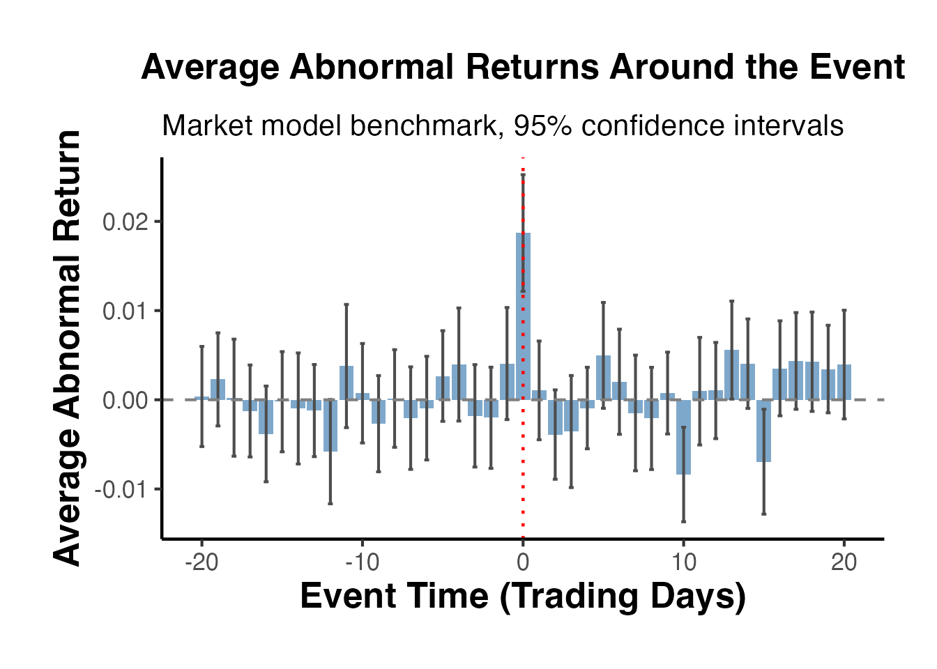
The plot should show a clear spike at (the event day), with smaller effects at (information leakage) and (post-announcement drift), consistent with our data generating process.
5. Cumulative Abnormal Returns (CAR)
5.1 Computing CAR for Individual Firms
The CAR for firm over window is the sum of abnormal returns across event days within that window.
# Compute CAR for each firm over several windows
compute_car <- function(data, tau1, tau2) {
    data %>%
        filter(event_time >= tau1 & event_time <= tau2) %>%
        group_by(firm_id) %>%
        dplyr::summarise(
            car        = sum(ar),
            window     = paste0("(", tau1, ",", tau2, ")"),
            .groups    = "drop"
        )
}

# Compute CARs for standard windows
car_1_1   <- compute_car(sim_data, -1, 1)
car_5_5   <- compute_car(sim_data, -5, 5)
car_10_10 <- compute_car(sim_data, -10, 10)
car_0_0   <- compute_car(sim_data, 0, 0)

# Combine all windows
all_cars <- bind_rows(car_1_1, car_5_5, car_10_10, car_0_0)

# Summary statistics by window
car_summary <- all_cars %>%
    group_by(window) %>%
    dplyr::summarise(
        mean_car   = mean(car),
        median_car = median(car),
        sd_car     = sd(car),
        n          = n(),
        t_stat     = mean(car) / (sd(car) / sqrt(n())),
        p_value    = 2 * (1 - pt(abs(t_stat), df = n() - 1)),
        .groups    = "drop"
    )

car_summary
#> # A tibble: 4 × 7
#>   window   mean_car median_car sd_car     n t_stat     p_value
#>   <chr>       <dbl>      <dbl>  <dbl> <int>  <dbl>       <dbl>
#> 1 (-1,1)    0.0238      0.0230 0.0404    50  4.17  0.000123
#> 2 (-10,10)  0.00925     0.0302 0.104     50  0.626 0.534
#> 3 (-5,5)    0.0232      0.0307 0.0797    50  2.06  0.0449
#> 4 (0,0)     0.0187      0.0181 0.0236    50  5.60  0.000000960
5.2 Cumulative Average Abnormal Return Over Time
We can also track how the cumulative abnormal return builds up over the event window by computing a running sum of the average AR.
# Compute cumulative average abnormal return (CAAR)
caar <- avg_ar %>%
    arrange(event_time) %>%
    mutate(
        caar    = cumsum(mean_ar),
        caar_se = sqrt(cumsum(se_ar^2))
    )

head(caar, 10)
#> # A tibble: 10 × 6
#>    event_time   mean_ar   se_ar n_firms      caar caar_se
#>         <dbl>     <dbl>   <dbl>   <int>     <dbl>   <dbl>
#>  1        -20  0.000370 0.00286      50  0.000370 0.00286
#>  2        -19  0.00229  0.00266      50  0.00266  0.00391
#>  3        -18  0.000238 0.00335      50  0.00289  0.00515
#>  4        -17 -0.00125  0.00263      50  0.00164  0.00578
#>  5        -16 -0.00383  0.00274      50 -0.00219  0.00640
#>  6        -15 -0.000216 0.00287      50 -0.00240  0.00701
#>  7        -14 -0.000973 0.00318      50 -0.00338  0.00769
#>  8        -13 -0.00121  0.00263      50 -0.00458  0.00813
#>  9        -12 -0.00581  0.00298      50 -0.0104   0.00866
#> 10        -11  0.00378  0.00352      50 -0.00661  0.00935
5.3 Visualizing CAAR
ggplot(caar, aes(x = event_time, y = caar)) +
    geom_ribbon(aes(ymin = caar - 1.96 * caar_se,
                    ymax = caar + 1.96 * caar_se),
                fill = "steelblue", alpha = 0.2) +
    geom_line(color = "steelblue", linewidth = 1) +
    geom_point(color = "steelblue", size = 1.5) +
    geom_hline(yintercept = 0, linetype = "dashed", color = "grey50") +
    geom_vline(xintercept = 0, linetype = "dotted", color = "red", linewidth = 0.8) +
    labs(
        title    = "Cumulative Average Abnormal Return (CAAR)",
        subtitle = "Market model benchmark, 95% confidence band",
        x        = "Event Time (Trading Days)",
        y        = "CAAR"
    ) +
    causalverse::ama_theme()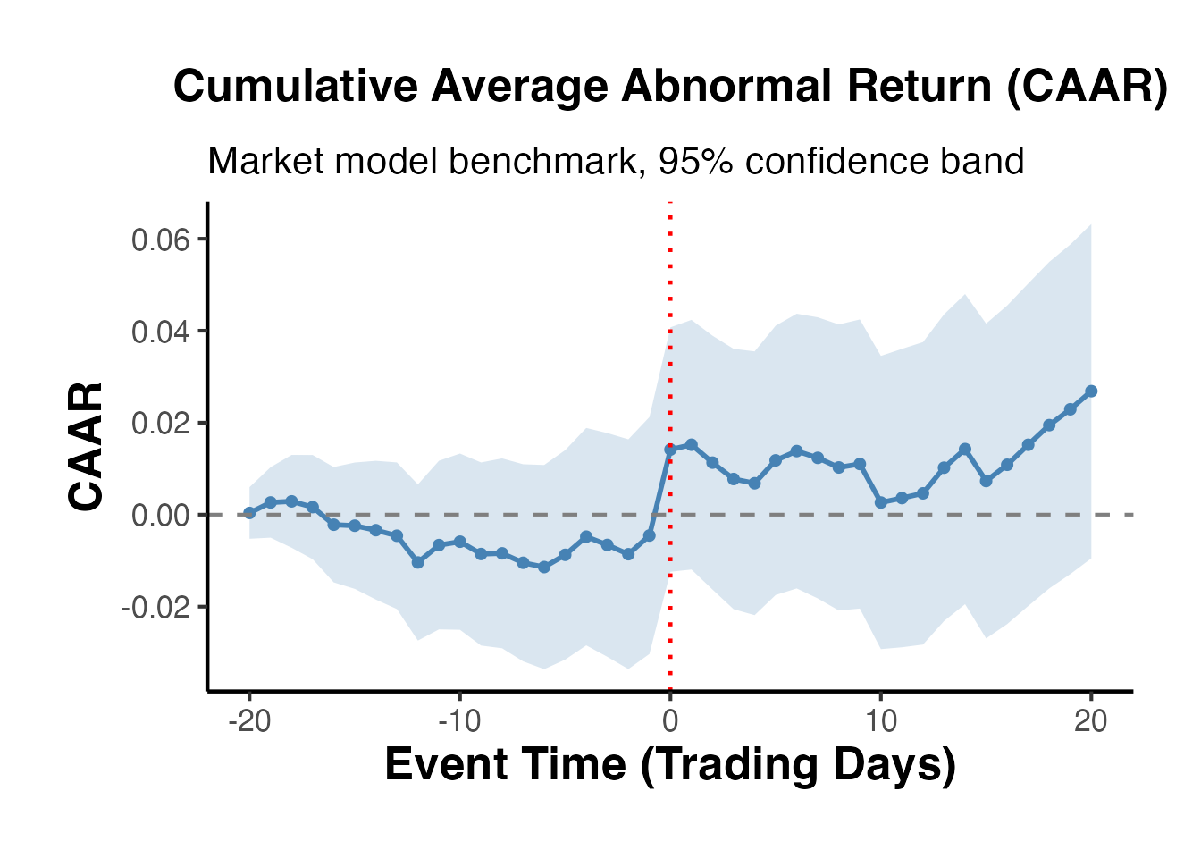
The CAAR plot is the classic output of a finance event study. We expect to see a relatively flat line before the event, a sharp jump at the event date, and a plateau afterward (if the market is efficient and there is no post-event drift).
5.4 CAR Distribution Across Firms
ggplot(car_1_1, aes(x = car)) +
    geom_histogram(bins = 20, fill = "steelblue", color = "white", alpha = 0.8) +
    geom_vline(xintercept = mean(car_1_1$car),
               linetype = "dashed", color = "red", linewidth = 0.8) +
    labs(
        title    = "Distribution of CAR(-1, +1) Across Firms",
        subtitle = paste("Mean CAR =", round(mean(car_1_1$car), 4)),
        x        = "CAR(-1, +1)",
        y        = "Count"
    ) +
    causalverse::ama_theme()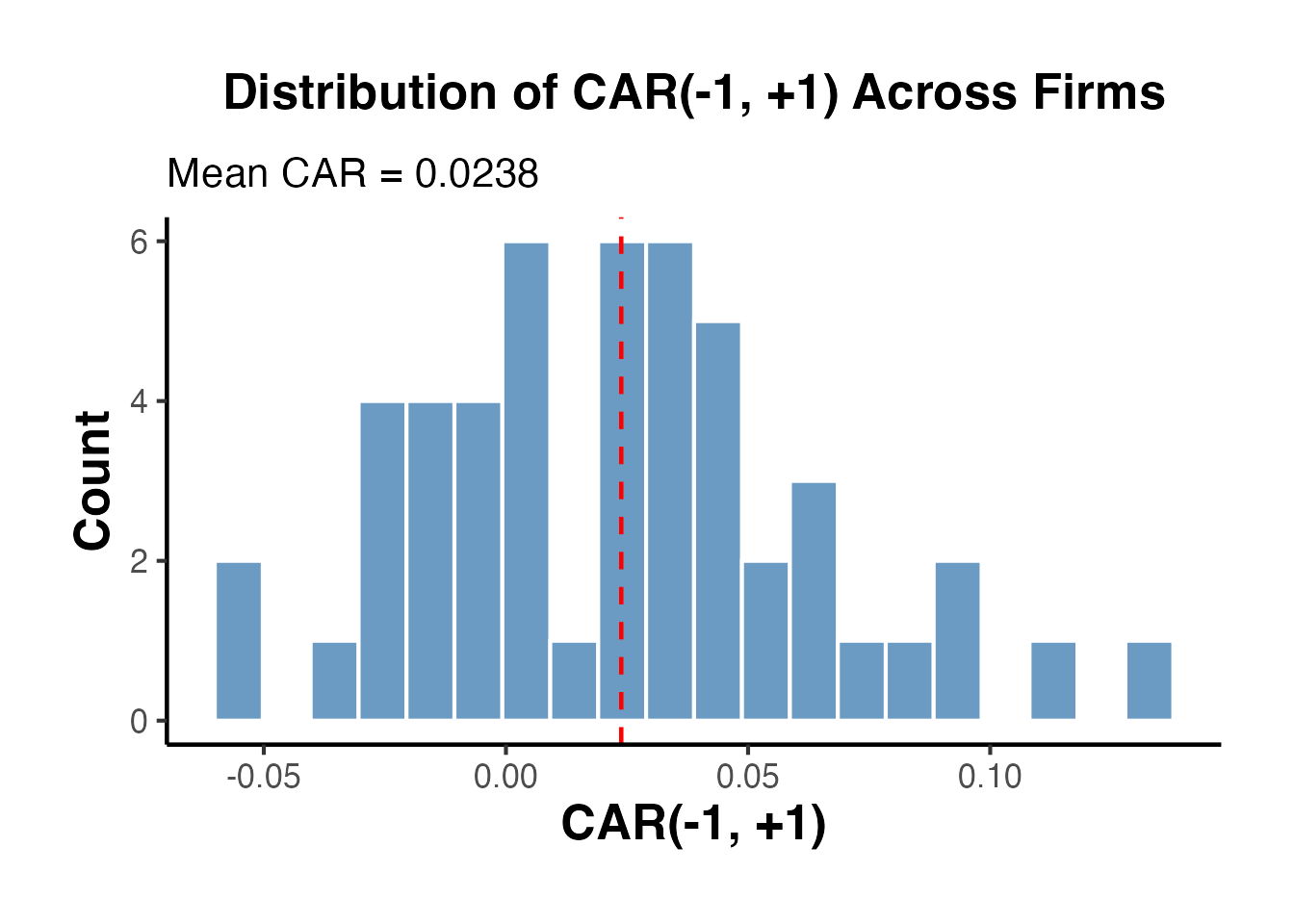
6. Statistical Tests
A central concern in event studies is whether the observed abnormal returns are statistically different from zero. Several parametric and non-parametric tests have been developed for this purpose.
6.1 Parametric Tests
6.1.1 Cross-Sectional t-Test
The simplest test computes the t-statistic from the cross-section of CARs:
where is the cross-sectional standard deviation of CARs and is the number of events.
# Cross-sectional t-test on CAR(-1,+1)
car_values <- car_1_1$car
n          <- length(car_values)
mean_car   <- mean(car_values)
sd_car     <- sd(car_values)
t_stat_cs  <- mean_car / (sd_car / sqrt(n))
p_value_cs <- 2 * (1 - pt(abs(t_stat_cs), df = n - 1))

cat("Cross-Sectional t-Test for CAR(-1,+1)\n")
#> Cross-Sectional t-Test for CAR(-1,+1)
cat("--------------------------------------\n")
#> --------------------------------------
cat("Mean CAR:   ", round(mean_car, 6), "\n")
#> Mean CAR:    0.02381
cat("Std Dev:    ", round(sd_car, 6), "\n")
#> Std Dev:     0.040367
cat("N:          ", n, "\n")
#> N:           50
cat("t-statistic:", round(t_stat_cs, 4), "\n")
#> t-statistic: 4.1708
cat("p-value:    ", format.pval(p_value_cs, digits = 4), "\n")
#> p-value:     0.0001234
6.1.2 Standardized Cross-Sectional Test (Patell Test)
The Patell (1976) test standardizes each firm’s abnormal return by its own estimation-period standard deviation before averaging. This accounts for differences in return volatility across firms:
where is the length of the estimation window and the adjustment factor corrects for forecast error.
# Compute standardized abnormal returns (simplified Patell approach)
est_sigmas <- model_params$sigma  # estimation-window residual std dev

# For each firm, compute standardized CAR
standardized_cars <- sapply(1:n_firms, function(i) {
    firm_ar <- sim_data %>%
        filter(firm_id == i, event_time >= -1 & event_time <= 1) %>%
        pull(ar)

    # Sum of ARs over the window
    car_i <- sum(firm_ar)

    # Standard deviation under Patell (simplified: sigma * sqrt(L_event))
    L_event <- length(firm_ar)
    sd_car_i <- est_sigmas[i] * sqrt(L_event)

    # Standardized CAR
    car_i / sd_car_i
})

# Patell test statistic
t_patell  <- mean(standardized_cars) * sqrt(n_firms)
p_patell  <- 2 * (1 - pnorm(abs(t_patell)))

cat("Patell (1976) Standardized Test\n")
#> Patell (1976) Standardized Test
cat("-------------------------------\n")
#> -------------------------------
cat("Average SCAR:", round(mean(standardized_cars), 4), "\n")
#> Average SCAR: 0.6887
cat("Z-statistic: ", round(t_patell, 4), "\n")
#> Z-statistic:  4.8701
cat("p-value:     ", format.pval(p_patell, digits = 4), "\n")
#> p-value:      1.115e-06
6.1.3 BMP Test (Boehmer, Musumeci, and Poulsen, 1991)
The BMP test combines the Patell standardization with a cross-sectional variance estimate. This makes it robust to event-induced increases in variance, which is a common problem when events themselves affect stock return volatility:
# BMP test
mean_scar  <- mean(standardized_cars)
sd_scar    <- sd(standardized_cars)
t_bmp      <- (mean_scar / sd_scar) * sqrt(n_firms)
p_bmp      <- 2 * (1 - pnorm(abs(t_bmp)))

cat("BMP (1991) Test\n")
#> BMP (1991) Test
cat("---------------\n")
#> ---------------
cat("Mean SCAR:   ", round(mean_scar, 4), "\n")
#> Mean SCAR:    0.6887
cat("SD of SCARs: ", round(sd_scar, 4), "\n")
#> SD of SCARs:  1.1796
cat("t-statistic: ", round(t_bmp, 4), "\n")
#> t-statistic:  4.1285
cat("p-value:     ", format.pval(p_bmp, digits = 4), "\n")
#> p-value:      3.651e-05
6.2 Non-Parametric Tests
Non-parametric tests are valuable because they do not rely on the assumption that abnormal returns are normally distributed, which is often violated with daily stock return data.
6.2.1 Sign Test
The sign test examines whether the fraction of positive CARs exceeds 50%. Under the null hypothesis of no abnormal performance, the number of positive CARs follows a binomial distribution:
# Sign test
n_positive <- sum(car_values > 0)
n_total    <- length(car_values)

# Under H0, p = 0.5
# Use exact binomial test
sign_test <- binom.test(n_positive, n_total, p = 0.5)

cat("Sign Test for CAR(-1,+1)\n")
#> Sign Test for CAR(-1,+1)
cat("------------------------\n")
#> ------------------------
cat("Positive CARs:", n_positive, "out of", n_total, "\n")
#> Positive CARs: 35 out of 50
cat("Proportion:   ", round(n_positive / n_total, 4), "\n")
#> Proportion:    0.7
cat("p-value:      ", format.pval(sign_test$p.value, digits = 4), "\n")
#> p-value:       0.0066
6.2.2 Generalized Sign Test
The generalized sign test adjusts the expected proportion of positive abnormal returns using the estimation window, rather than assuming 50%. The expected proportion is computed as the average fraction of positive abnormal returns across firms during the estimation window:
# Compute the expected proportion of positive ARs from the estimation window
est_positive_fractions <- sapply(1:n_firms, function(i) {
    firm_est <- sim_data %>%
        filter(firm_id == i, day >= est_start & day <= est_end)
    mean(firm_est$ar > 0)
})

p_hat <- mean(est_positive_fractions)

# Generalized sign test statistic
z_gsign <- (n_positive - n_total * p_hat) / sqrt(n_total * p_hat * (1 - p_hat))
p_gsign <- 2 * (1 - pnorm(abs(z_gsign)))

cat("Generalized Sign Test\n")
#> Generalized Sign Test
cat("---------------------\n")
#> ---------------------
cat("Expected p(AR > 0) from est. window:", round(p_hat, 4), "\n")
#> Expected p(AR > 0) from est. window: 0.5002
cat("Observed positive CARs:", n_positive, "\n")
#> Observed positive CARs: 35
cat("Z-statistic:", round(z_gsign, 4), "\n")
#> Z-statistic: 2.8251
cat("p-value:    ", format.pval(p_gsign, digits = 4), "\n")
#> p-value:     0.004727
6.2.3 Rank Test (Corrado, 1989)
The Corrado rank test transforms abnormal returns into ranks within each firm’s full time series. The test statistic is based on the deviation of the average rank on the event day from its expected value under the null:
# Corrado rank test
# For each firm, rank the abnormal returns across all days
rank_data <- sim_data %>%
    group_by(firm_id) %>%
    mutate(
        ar_rank     = rank(ar),
        n_days_firm = n(),
        centered_rank = (ar_rank - (n_days_firm + 1) / 2)
    ) %>%
    ungroup()

# Compute the average centered rank on the event day (event_time == 0)
event_day_ranks <- rank_data %>%
    filter(event_time == 0)

avg_rank <- mean(event_day_ranks$centered_rank)

# Standard deviation of average ranks (computed from all days in the sample)
rank_sd <- rank_data %>%
    group_by(day) %>%
    dplyr::summarise(daily_avg_rank = mean(centered_rank), .groups = "drop") %>%
    pull(daily_avg_rank) %>%
    sd()

t_corrado <- avg_rank / rank_sd
p_corrado <- 2 * (1 - pnorm(abs(t_corrado)))

cat("Corrado (1989) Rank Test\n")
#> Corrado (1989) Rank Test
cat("------------------------\n")
#> ------------------------
cat("Average centered rank on event day:", round(avg_rank, 4), "\n")
#> Average centered rank on event day: 64.42
cat("Rank std deviation:", round(rank_sd, 4), "\n")
#> Rank std deviation: 13.4108
cat("t-statistic:", round(t_corrado, 4), "\n")
#> t-statistic: 4.8036
cat("p-value:    ", format.pval(p_corrado, digits = 4), "\n")
#> p-value:     1.558e-06
6.3 Summary of Test Results
test_results <- data.frame(
    Test = c("Cross-sectional t-test",
             "Patell (1976)",
             "BMP (1991)",
             "Sign test",
             "Generalized sign test",
             "Corrado rank test"),
    Statistic = c(round(t_stat_cs, 4),
                  round(t_patell, 4),
                  round(t_bmp, 4),
                  paste0(n_positive, "/", n_total),
                  round(z_gsign, 4),
                  round(t_corrado, 4)),
    P_value = c(format.pval(p_value_cs, digits = 4),
                format.pval(p_patell, digits = 4),
                format.pval(p_bmp, digits = 4),
                format.pval(sign_test$p.value, digits = 4),
                format.pval(p_gsign, digits = 4),
                format.pval(p_corrado, digits = 4)),
    stringsAsFactors = FALSE
)

test_results
#>                     Test Statistic   P_value
#> 1 Cross-sectional t-test    4.1708 0.0001234
#> 2          Patell (1976)    4.8701 1.115e-06
#> 3             BMP (1991)    4.1285 3.651e-05
#> 4              Sign test     35/50    0.0066
#> 5  Generalized sign test    2.8251  0.004727
#> 6      Corrado rank test    4.8036 1.558e-06
7. Buy-and-Hold Abnormal Returns (BHAR)
7.1 Why BHAR?
For long-horizon event studies (e.g., measuring performance over 1-3 years following an IPO, SEO, or merger), cumulative abnormal returns can be misleading because they implicitly assume daily portfolio rebalancing. The buy-and-hold abnormal return compounds returns as an investor who buys on the event date and holds through the measurement horizon would actually experience.
7.2 BHAR Calculation
# Compute BHAR for each firm over the post-event period [0, +30]
bhar_data <- sim_data %>%
    filter(event_time >= 0 & event_time <= 30) %>%
    group_by(firm_id) %>%
    arrange(event_time) %>%
    mutate(
        cum_ret     = cumprod(1 + ret) - 1,
        cum_mkt_ret = cumprod(1 + market_ret) - 1
    ) %>%
    ungroup()

# BHAR for each firm at the end of the window
bhar_final <- bhar_data %>%
    filter(event_time == 30) %>%
    mutate(bhar = cum_ret - cum_mkt_ret)

cat("BHAR(0, +30) Summary\n")
#> BHAR(0, +30) Summary
cat("--------------------\n")
#> --------------------
cat("Mean BHAR:  ", round(mean(bhar_final$bhar), 6), "\n")
#> Mean BHAR:   0.044272
cat("Median BHAR:", round(median(bhar_final$bhar), 6), "\n")
#> Median BHAR: 0.038424
cat("Std Dev:    ", round(sd(bhar_final$bhar), 6), "\n")
#> Std Dev:     0.120726

# t-test on BHAR
t_bhar <- t.test(bhar_final$bhar, mu = 0)
cat("t-statistic:", round(t_bhar$statistic, 4), "\n")
#> t-statistic: 2.5931
cat("p-value:    ", format.pval(t_bhar$p.value, digits = 4), "\n")
#> p-value:     0.01251
7.3 BHAR Accumulation Over Time
# Average BHAR over time
avg_bhar <- bhar_data %>%
    group_by(event_time) %>%
    dplyr::summarise(
        mean_bhar = mean(cum_ret - cum_mkt_ret),
        se_bhar   = sd(cum_ret - cum_mkt_ret) / sqrt(n()),
        .groups   = "drop"
    )

ggplot(avg_bhar, aes(x = event_time, y = mean_bhar)) +
    geom_ribbon(aes(ymin = mean_bhar - 1.96 * se_bhar,
                    ymax = mean_bhar + 1.96 * se_bhar),
                fill = "darkorange", alpha = 0.2) +
    geom_line(color = "darkorange", linewidth = 1) +
    geom_hline(yintercept = 0, linetype = "dashed", color = "grey50") +
    labs(
        title    = "Average BHAR Over Post-Event Window",
        subtitle = "Market-adjusted, 95% confidence band",
        x        = "Event Time (Trading Days)",
        y        = "Average BHAR"
    ) +
    causalverse::ama_theme()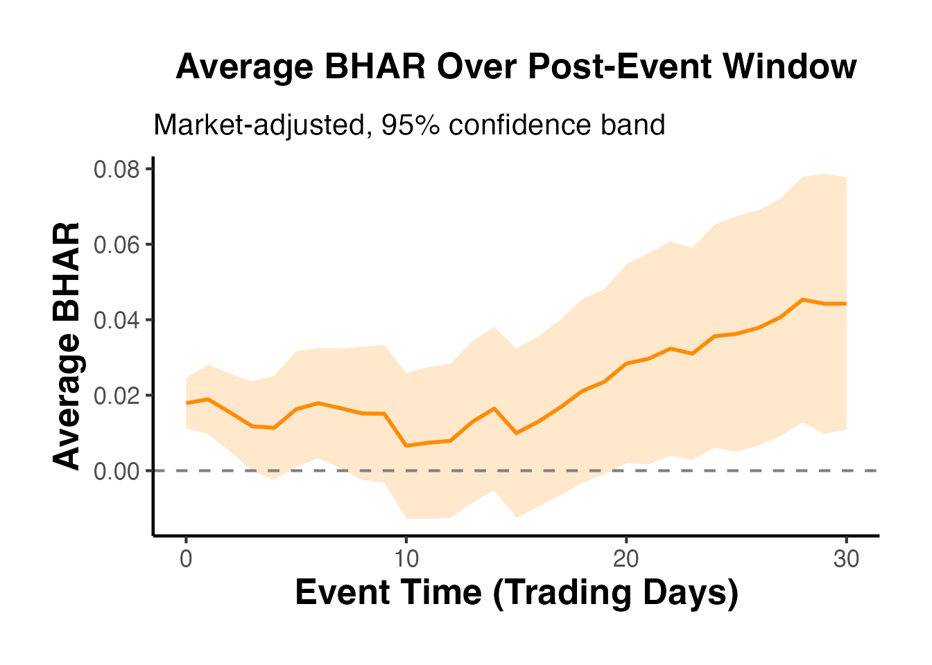
7.4 Calendar-Time Portfolio Approach (CTAR)
An alternative to BHAR for long-horizon studies is the calendar-time portfolio approach (also called the calendar-time abnormal return, CTAR). Rather than aligning returns in event time, this method forms a portfolio each calendar month that includes all firms that have experienced an event within the prior months. The portfolio return is then regressed on factor models:
The intercept (Jensen’s alpha) measures average monthly abnormal performance. The advantage of CTAR is that it accounts for cross-sectional dependence among event firms (because overlapping event windows are aggregated into a single portfolio return), whereas BHAR tests can overstate statistical significance when events cluster in calendar time.
We illustrate the concept with our simulated data by forming daily portfolios:
# Calendar-time portfolio: for each calendar day, compute the
# equal-weighted return of all firms in their post-event window [0, +20]
ctar_data <- sim_data %>%
    filter(event_time >= 0 & event_time <= 20)

# Equal-weighted portfolio return each day
ctar_portfolio <- ctar_data %>%
    group_by(day) %>%
    dplyr::summarise(
        port_ret   = mean(ret),
        port_mkt   = mean(market_ret),
        n_firms    = n(),
        .groups    = "drop"
    )

# Regress portfolio excess returns on market returns
ctar_model <- lm(port_ret ~ port_mkt, data = ctar_portfolio)

cat("Calendar-Time Portfolio Regression\n")
#> Calendar-Time Portfolio Regression
cat("-----------------------------------\n")
#> -----------------------------------
cat("Alpha (intercept):", round(coef(ctar_model)[1], 6), "\n")
#> Alpha (intercept): 0.000883
cat("t-stat on alpha:  ", round(summary(ctar_model)$coefficients[1, 3], 4), "\n")
#> t-stat on alpha:   0.8787
cat("Beta:             ", round(coef(ctar_model)[2], 4), "\n")
#> Beta:              0.679
cat("R-squared:        ", round(summary(ctar_model)$r.squared, 4), "\n")
#> R-squared:         0.6678
8. Fama-French Factor Models
In practice, researchers use the Fama-French factor data available from Kenneth French’s data library. The three-factor and four-factor models provide more precise benchmarks for expected returns than the simple market model.
8.1 Three-Factor Model
The Fama-French (1993) three-factor model accounts for the well-documented size and value premiums:
# Download Fama-French 3-factor data using the frenchdata package
library(frenchdata)
ff3_raw <- download_french_data("Fama/French 3 Factors (Daily)")
ff3 <- ff3_raw$subsets$data[[1]]

# Clean up: convert date, scale factors from percent to decimal
ff3 <- ff3 %>%
    mutate(
        date   = as.Date(as.character(date), format = "%Y%m%d"),
        mkt_rf = `Mkt-RF` / 100,
        smb    = SMB / 100,
        hml    = HML / 100,
        rf     = RF / 100
    ) %>%
    dplyr::select(date, mkt_rf, smb, hml, rf) %>%
    filter(!is.na(date))

# --- Simulate stock return data to merge with the factor data ---
set.seed(123)
n_days_ff   <- min(500, nrow(ff3))
ff3_subset  <- tail(ff3, n_days_ff)
event_day_ff <- round(n_days_ff * 0.7)

stock_data <- data.frame(
    date       = ff3_subset$date,
    ret        = 0.0003 + 1.1 * ff3_subset$mkt_rf +
                 0.3 * ff3_subset$smb - 0.2 * ff3_subset$hml +
                 rnorm(n_days_ff, 0, 0.01),
    event_time = seq_len(n_days_ff) - event_day_ff,
    stringsAsFactors = FALSE
)

# Inject an event effect
stock_data$ret[stock_data$event_time == 0] <-
    stock_data$ret[stock_data$event_time == 0] + 0.02

# Merge factor data with stock returns
merged_data <- merge(stock_data, ff3_subset, by = "date")
merged_data$excess_ret <- merged_data$ret - merged_data$rf

# Estimation window regression (event_time < -20)
ff3_model <- lm(
    excess_ret ~ mkt_rf + smb + hml,
    data = merged_data[merged_data$event_time < -20, ]
)

# Abnormal return in event window
merged_data$ar_ff3 <- merged_data$excess_ret -
    predict(ff3_model, newdata = merged_data)

# Show event-window abnormal returns
merged_data %>%
    filter(event_time >= -5 & event_time <= 5) %>%
    dplyr::select(date, event_time, ret, excess_ret, ar_ff3) %>%
    print()

summary(ff3_model)
8.2 Carhart Four-Factor Model
The Carhart (1997) model adds a momentum factor, which captures the tendency of past winners to continue outperforming and past losers to continue underperforming:
# Download Carhart / momentum factor data
library(frenchdata)
mom_raw <- download_french_data("F-F Momentum Factor (daily)")
mom     <- mom_raw$subsets$data[[1]]

mom <- mom %>%
    mutate(
        date = as.Date(as.character(date), format = "%Y%m%d"),
        umd  = Mom / 100
    ) %>%
    dplyr::select(date, umd) %>%
    filter(!is.na(date))

# Merge momentum factor into merged_data created in the FF3 chunk
merged_data <- merge(merged_data, mom, by = "date", all.x = TRUE)
merged_data <- merged_data[!is.na(merged_data$umd), ]

# Carhart 4-factor estimation window regression
ff4_model <- lm(
    excess_ret ~ mkt_rf + smb + hml + umd,
    data = merged_data[merged_data$event_time < -20, ]
)

# Abnormal return
merged_data$ar_ff4 <- merged_data$excess_ret -
    predict(ff4_model, newdata = merged_data)

# The four-factor model is especially important for long-horizon studies
# where momentum effects can confound abnormal return estimates.

# Show event-window abnormal returns
merged_data %>%
    filter(event_time >= -5 & event_time <= 5) %>%
    dplyr::select(date, event_time, ar_ff3, ar_ff4) %>%
    print()

summary(ff4_model)
8.3 Which Model to Use?
The choice of normal return model depends on the research context:
- Short-window studies (3-5 days): The market model is generally sufficient. Brown and Warner (1985) showed that more complex models add little power for short windows because the variance of abnormal returns is dominated by the firm-specific component.
- Long-window studies (months to years): Factor models are recommended because size, value, and momentum characteristics can systematically bias abnormal returns over longer horizons (Fama, 1998; Mitchell and Stafford, 2000).
- Cross-sectional variation: When event firms have systematically different risk characteristics from the market (e.g., small firms, high book-to-market firms), factor models provide a better benchmark.
9. The EventStudy Package
The EventStudy R package provides a comprehensive implementation of event study methodology, including multiple return models and statistical tests.
9.1 Basic Usage
library(EventStudy)

# The EventStudy package requires three input files:
# 1. Request file: specifying parameters
# 2. Firm data: stock returns indexed by date
# 3. Market data: market/factor returns indexed by date

# Example setup:
# est_setup <- EventStudyAPI$new()
# est_setup$authentication(apiKey = "your_api_key")

# --- Prepare simulated data in the format EventStudy expects ---
# Create date sequence for our simulated data
sim_dates <- seq.Date(as.Date("2022-01-03"), by = "day", length.out = n_days)
sim_dates <- sim_dates[!weekdays(sim_dates) %in% c("Saturday", "Sunday")]
sim_dates <- sim_dates[seq_len(n_days)]

# Firm returns: columns = date + one column per firm
firm_returns_wide <- sim_data %>%
    filter(firm_id <= 5) %>%
    mutate(date = sim_dates[day]) %>%
    dplyr::select(date, firm_id, ret) %>%
    tidyr::pivot_wider(names_from = firm_id, values_from = ret,
                       names_prefix = "firm_")

# Market returns
market_returns_df <- data.frame(
    date       = sim_dates,
    market_ret = market_ret
)

# Event list: firm name, event date, group
event_list_df <- data.frame(
    firm  = paste0("firm_", 1:5),
    date  = sim_dates[event_day],
    group = "group1",
    stringsAsFactors = FALSE
)

cat("Firm returns (first 5 rows):\n")
print(head(firm_returns_wide, 5))
cat("\nEvent list:\n")
print(event_list_df)

# Note: Full EventStudy::EventStudy() usage depends on API key or
# specific local computation functions available in the package version.
# Consult the EventStudy package documentation for the exact syntax.
9.2 Available Models in EventStudy
The package supports several return models:
-
Market model:
model = "market_model" -
Market-adjusted model:
model = "market_adjusted" -
Mean-adjusted model:
model = "mean_adjusted" -
Fama-French three-factor:
model = "ff3" -
Carhart four-factor:
model = "ff4"
9.3 Available Tests in EventStudy
The package implements a comprehensive set of parametric and non-parametric tests:
- Parametric: t-test, Patell test, BMP test, standardized residual test
- Non-parametric: Sign test, generalized sign test, Corrado rank test, Wilcoxon signed-rank test
# Demonstrate the types of results the EventStudy package provides.
# Since the API-based workflow requires authentication, we illustrate
# using our previously computed results from the simulated data.

# Access test results (from our manual pipeline above)
cat("=== Test Results (from manual pipeline) ===\n")
print(test_results)

cat("\n=== CAR Summary by Window ===\n")
print(car_summary)

# Cross-sectional regression on CARs
# (Using our simulated firm characteristics as stand-in for analyst coverage, etc.)
cross_section <- lm(
    car ~ log_mcap + leverage + roa,
    data = car_cross
)
summary(cross_section)
10. Cross-Sectional Analysis of CARs
10.1 Motivation
A natural follow-up question in event studies is: why do some firms experience larger abnormal returns than others? Cross-sectional analysis regresses individual firm CARs on firm characteristics to identify determinants of the market’s reaction.
Common explanatory variables include:
- Firm size (log market capitalization): smaller firms may have larger price reactions due to lower information environments.
- Leverage: highly leveraged firms may have amplified equity reactions to news.
- Profitability (ROA, ROE): profitable firms may receive different market reactions.
- Analyst coverage: firms followed by fewer analysts may have larger abnormal returns due to greater information asymmetry.
- Event-specific variables: deal premium in M&A, earnings surprise magnitude, regulatory severity.
10.2 OLS Cross-Sectional Regression
# Merge CARs with firm characteristics
car_cross <- car_1_1 %>%
    left_join(firm_chars, by = "firm_id")

# OLS regression of CAR on firm characteristics
cs_model_ols <- lm(car ~ log_mcap + leverage + roa, data = car_cross)

summary(cs_model_ols)
#>
#> Call:
#> lm(formula = car ~ log_mcap + leverage + roa, data = car_cross)
#>
#> Residuals:
#>       Min        1Q    Median        3Q       Max
#> -0.088473 -0.018639 -0.004599  0.010909  0.084254
#>
#> Coefficients:
#>              Estimate Std. Error t value Pr(>|t|)
#> (Intercept) -0.012930   0.033578  -0.385  0.70196
#> log_mcap     0.002235   0.003399   0.658  0.51413
#> leverage    -0.018561   0.030052  -0.618  0.53985
#> roa          0.497158   0.165387   3.006  0.00428 **
#> ---
#> Signif. codes:  0 '***' 0.001 '**' 0.01 '*' 0.05 '.' 0.1 ' ' 1
#>
#> Residual standard error: 0.03802 on 46 degrees of freedom
#> Multiple R-squared:  0.1671, Adjusted R-squared:  0.1127
#> F-statistic: 3.075 on 3 and 46 DF,  p-value: 0.03678
10.3 Using fixest::feols()
For robust standard errors and more flexible specifications, fixest::feols() is preferred:
# Cross-sectional regression with heteroskedasticity-robust SEs
cs_model_fixest <- feols(
    car ~ log_mcap + leverage + roa,
    data = car_cross,
    vcov = "hetero"
)

summary(cs_model_fixest)
#> OLS estimation, Dep. Var.: car
#> Observations: 50
#> Standard-errors: Heteroskedasticity-robust
#>              Estimate Std. Error   t value  Pr(>|t|)
#> (Intercept) -0.012930   0.031410 -0.411647 0.6825100
#> log_mcap     0.002235   0.003008  0.742893 0.4613234
#> leverage    -0.018561   0.030078 -0.617118 0.5401998
#> roa          0.497158   0.163787  3.035394 0.0039455 **
#> ---
#> Signif. codes:  0 '***' 0.001 '**' 0.01 '*' 0.05 '.' 0.1 ' ' 1
#> RMSE: 0.036471   Adj. R2: 0.112733
10.4 Interpreting Cross-Sectional Results
# Visualize the relationship between firm size and CAR
ggplot(car_cross, aes(x = log_mcap, y = car)) +
    geom_point(alpha = 0.6, color = "steelblue", size = 2) +
    geom_smooth(method = "lm", se = TRUE, color = "red",
                fill = "red", alpha = 0.15) +
    geom_hline(yintercept = 0, linetype = "dashed", color = "grey50") +
    labs(
        title = "CAR(-1,+1) vs. Firm Size",
        x     = "Log Market Capitalization",
        y     = "CAR(-1, +1)"
    ) +
    causalverse::ama_theme()
#> `geom_smooth()` using formula = 'y ~ x'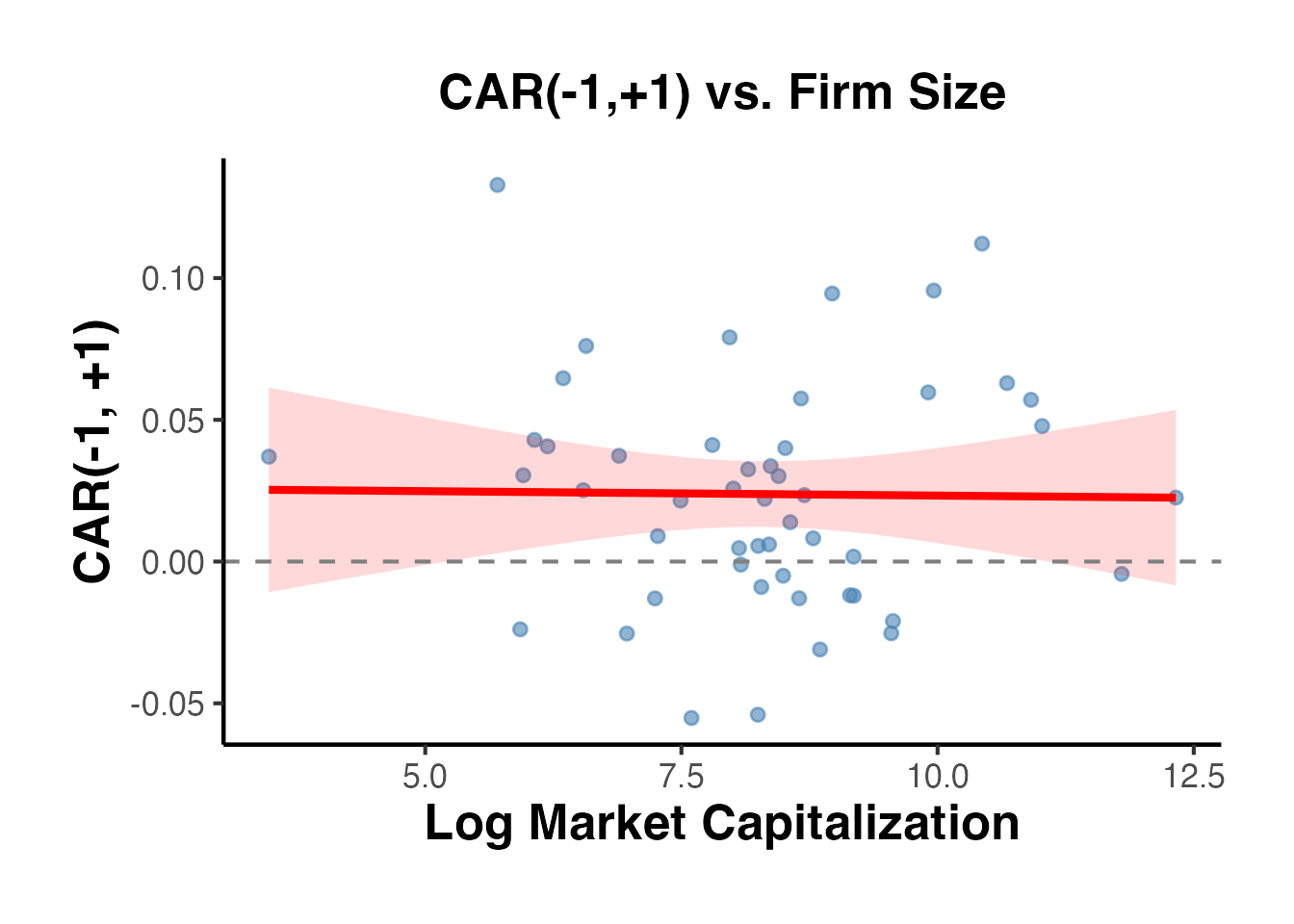
# Visualize the relationship between leverage and CAR
ggplot(car_cross, aes(x = leverage, y = car)) +
    geom_point(alpha = 0.6, color = "darkorange", size = 2) +
    geom_smooth(method = "lm", se = TRUE, color = "red",
                fill = "red", alpha = 0.15) +
    geom_hline(yintercept = 0, linetype = "dashed", color = "grey50") +
    labs(
        title = "CAR(-1,+1) vs. Leverage",
        x     = "Leverage (Debt/Assets)",
        y     = "CAR(-1, +1)"
    ) +
    causalverse::ama_theme()
#> `geom_smooth()` using formula = 'y ~ x'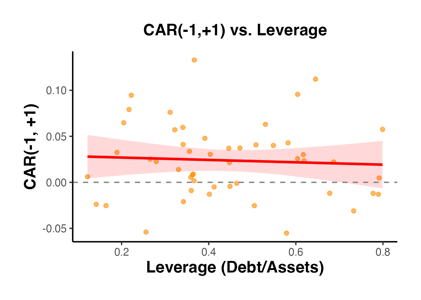
10.5 Multiple Window Analysis
Researchers sometimes run cross-sectional regressions for multiple event windows to check robustness:
# Run cross-sectional regression for each window
windows <- list(
    list(tau1 = 0,   tau2 = 0,   label = "(0,0)"),
    list(tau1 = -1,  tau2 = 1,   label = "(-1,+1)"),
    list(tau1 = -5,  tau2 = 5,   label = "(-5,+5)"),
    list(tau1 = -10, tau2 = 10,  label = "(-10,+10)")
)

multi_window_results <- lapply(windows, function(w) {
    cars <- compute_car(sim_data, w$tau1, w$tau2)
    cars <- merge(cars, firm_chars, by = "firm_id")
    model <- feols(car ~ log_mcap + leverage + roa, data = cars, vcov = "hetero")
    data.frame(
        window     = w$label,
        intercept  = round(coef(model)[1], 6),
        log_mcap   = round(coef(model)[2], 6),
        leverage   = round(coef(model)[3], 6),
        roa        = round(coef(model)[4], 6),
        n          = nobs(model),
        r_sq       = round(r2(model)["r2"], 4),
        stringsAsFactors = FALSE
    )
})

do.call(rbind, multi_window_results)
#>                 window intercept log_mcap  leverage      roa  n   r_sq
#> (Intercept)      (0,0) -0.007853 0.002493 -0.024962 0.318235 50 0.2256
#> (Intercept)1   (-1,+1) -0.012930 0.002235 -0.018561 0.497158 50 0.1671
#> (Intercept)2   (-5,+5) -0.100341 0.011700 -0.033798 0.781031 50 0.1319
#> (Intercept)3 (-10,+10) -0.089638 0.012260 -0.071900 0.546124 50 0.0632
11. The estudy2 Package: C++ Optimized Event Study Tests
The estudy2 package provides a high-performance, C++-optimized implementation of both parametric and nonparametric event study tests. It is particularly useful when you need to apply a comprehensive battery of statistical tests to your event study results, as it bundles 12 well-known test statistics into a single function call.
11.1 Overview of Available Tests
Parametric tests (6 total):
- Brown and Warner (1980) – the classic cross-sectional test using the mean and variance of abnormal returns across firms.
- Brown and Warner (1985) – extends the 1980 test to daily data with adjustments for estimation-period variance.
- Patell (1976) – standardizes each firm’s abnormal return by its own estimation-period standard deviation.
- Kolari and Pynnonen (2010) – adjusts the Patell test for cross-sectional correlation of abnormal returns.
- Boehmer, Musumeci, and Poulsen (1991) (BMP) – a standardized cross-sectional test robust to event-induced variance.
- Adjusted BMP (Kolari and Pynnonen, 2010) – further adjusts BMP for cross-correlation.
Nonparametric tests (6 total):
- Corrado (1989) rank test – ranks abnormal returns across the combined estimation and event windows.
- Corrado and Zivney (1992) – a sign test variant that accounts for the skewness of abnormal returns.
- Adjusted Corrado rank test (Kolari and Pynnonen, 2011) – corrects for cross-sectional dependence.
- Adjusted Corrado and Zivney sign test – the sign test analog adjusted for dependence.
- Generalized rank test (Kolari and Pynnonen, 2011) – a GRANK test that combines rank and t-test properties.
- Generalized sign test – tests whether the proportion of positive abnormal returns exceeds that expected under the null.
11.2 Basic Usage with estudy()
library(estudy2)
set.seed(42)

# Simulate returns for 30 firms over 300 trading days
n_firms <- 30
n_days  <- 300
dates   <- seq.Date(as.Date("2023-01-02"), by = "day", length.out = n_days)

# Market returns
market_ret <- rnorm(n_days, mean = 0.0004, sd = 0.012)

# Individual firm returns: market model + firm-specific noise
firm_returns <- lapply(1:n_firms, function(i) {
    beta_i  <- runif(1, 0.7, 1.4)
    alpha_i <- rnorm(1, 0, 0.0002)
    eps_i   <- rnorm(n_days, 0, 0.015)
    ret     <- alpha_i + beta_i * market_ret + eps_i
    # Inject an event effect on day 250 for all firms
    ret[250] <- ret[250] + rnorm(1, 0.02, 0.005)
    zoo::zoo(ret, order.by = dates)
})
market_zoo <- zoo::zoo(market_ret, order.by = dates)

# Run the full battery of event study tests
#   event_start / event_end define the event window (relative to the list index)
result <- estudy2::estudy(
    list_of_returns = firm_returns,
    market_return   = market_zoo,
    event_start     = -2,
    event_end       = 2
)

# Display parametric test results
cat("=== Parametric Test Results ===\n")
print(head(result$parametric))
11.3 Interpreting Nonparametric Results
Nonparametric tests are especially valuable when abnormal returns are non-normal (e.g., skewed or heavy-tailed), which is common in daily stock return data. The Corrado rank test and the generalized rank (GRANK) test are often recommended as robust alternatives to parametric tests in applied work.
12. Long-Horizon Event Studies
Short-window event studies (1–5 days) are the gold standard for measuring the market’s immediate reaction to an event. However, many research questions require examining long-horizon abnormal performance over months or years – for example, post-merger integration effects, post-IPO performance, or the long-run consequences of regulatory changes.
12.1 Calendar-Time Portfolio Approach (CTPR)
The calendar-time portfolio regression (CTPR) method (Jaffe, 1974; Mitchell and Stafford, 2000) forms a portfolio each calendar month consisting of all firms that experienced the event within a specified prior window (e.g., the past 12 months). The portfolio’s excess returns are then regressed on factor models (CAPM, Fama-French three-factor, etc.), and the intercept (alpha) measures the average monthly abnormal return.
set.seed(42)

# Simulate monthly returns for 50 firms over 60 months
n_firms  <- 50
n_months <- 60
months   <- seq.Date(as.Date("2019-01-01"), by = "month", length.out = n_months)

# Factor returns
mkt_rf <- rnorm(n_months, 0.006, 0.045)
smb    <- rnorm(n_months, 0.002, 0.030)
hml    <- rnorm(n_months, 0.003, 0.028)
rf     <- rep(0.002 / 12, n_months)

# Each firm has a random event month between months 13 and 36
event_months <- sample(13:36, n_firms, replace = TRUE)

# Simulate firm returns: 3-factor model + post-event alpha
firm_data <- do.call(rbind, lapply(1:n_firms, function(i) {
    beta_m <- runif(1, 0.8, 1.3)
    beta_s <- runif(1, -0.3, 0.5)
    beta_h <- runif(1, -0.4, 0.4)
    eps    <- rnorm(n_months, 0, 0.04)
    ret    <- rf + beta_m * mkt_rf + beta_s * smb + beta_h * hml + eps
    # Add negative post-event drift of -0.5% per month
    post_event <- (1:n_months) > event_months[i] &
                  (1:n_months) <= (event_months[i] + 12)
    ret[post_event] <- ret[post_event] - 0.005
    data.frame(
        firm  = i,
        month = months,
        ret   = ret,
        in_portfolio = as.integer(
            (1:n_months) > event_months[i] &
            (1:n_months) <= (event_months[i] + 12)
        )
    )
}))

# Form calendar-time portfolio: equal-weighted average of event firms each month
ctpr_data <- firm_data |>
    dplyr::filter(in_portfolio == 1) |>
    dplyr::group_by(month) |>
    dplyr::summarise(port_ret = mean(ret), n_firms = dplyr::n(), .groups = "drop")

# Merge with factor data
ctpr_data$mkt_rf <- mkt_rf[match(ctpr_data$month, months)]
ctpr_data$smb    <- smb[match(ctpr_data$month, months)]
ctpr_data$hml    <- hml[match(ctpr_data$month, months)]
ctpr_data$rf     <- rf[match(ctpr_data$month, months)]
ctpr_data$excess <- ctpr_data$port_ret - ctpr_data$rf

# Regress on Fama-French three factors
ctpr_model <- lm(excess ~ mkt_rf + smb + hml, data = ctpr_data)
summary(ctpr_model)
#>
#> Call:
#> lm(formula = excess ~ mkt_rf + smb + hml, data = ctpr_data)
#>
#> Residuals:
#>       Min        1Q    Median        3Q       Max
#> -0.020285 -0.007660 -0.002236  0.008259  0.039837
#>
#> Coefficients:
#>               Estimate Std. Error t value Pr(>|t|)
#> (Intercept)  5.844e-05  2.175e-03   0.027    0.979
#> mkt_rf       1.040e+00  4.298e-02  24.208   <2e-16 ***
#> smb         -6.747e-02  7.990e-02  -0.844    0.405
#> hml          9.715e-02  9.414e-02   1.032    0.310
#> ---
#> Signif. codes:  0 '***' 0.001 '**' 0.01 '*' 0.05 '.' 0.1 ' ' 1
#>
#> Residual standard error: 0.01264 on 31 degrees of freedom
#> Multiple R-squared:  0.9515, Adjusted R-squared:  0.9468
#> F-statistic: 202.9 on 3 and 31 DF,  p-value: < 2.2e-16
The intercept (alpha) from this regression captures the average monthly abnormal return for event firms. A negative and significant alpha suggests post-event underperformance.
12.2 Buy-and-Hold Abnormal Returns (Long-Horizon)
For horizons of 12–36 months, the buy-and-hold abnormal return (BHAR) compounds returns and compares them against a benchmark:
set.seed(42)

# Simulate 36-month post-event returns for 40 firms
n_firms   <- 40
horizon   <- 36
benchmark <- rnorm(horizon, 0.008, 0.04)  # monthly benchmark returns

bhars <- sapply(1:n_firms, function(i) {
    firm_ret <- benchmark + rnorm(horizon, -0.003, 0.03)  # slight underperformance
    prod(1 + firm_ret) - prod(1 + benchmark)
})

bhar_df <- data.frame(firm = 1:n_firms, BHAR = bhars)

ggplot(bhar_df, aes(x = BHAR)) +
    geom_histogram(bins = 15, fill = "steelblue", color = "white", alpha = 0.8) +
    geom_vline(xintercept = mean(bhars), color = "red", linewidth = 1, linetype = "dashed") +
    labs(
        title    = "Distribution of 36-Month Buy-and-Hold Abnormal Returns",
        subtitle = paste0("Mean BHAR = ", round(mean(bhars), 4),
                          " | t = ", round(mean(bhars) / (sd(bhars) / sqrt(n_firms)), 2)),
        x = "BHAR", y = "Count"
    ) +
    causalverse::ama_theme()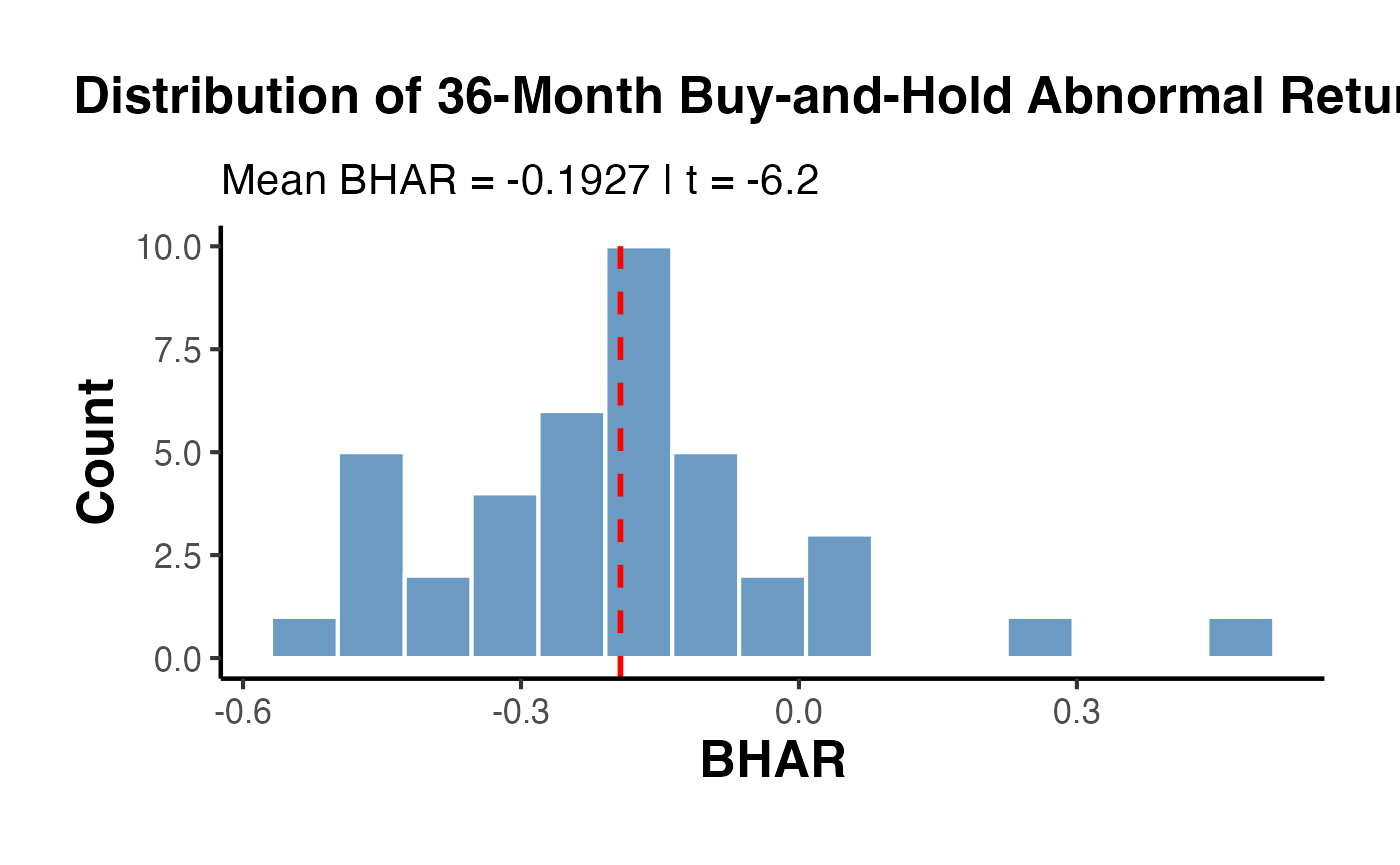
12.3 Robust Inference with crseEventStudy
The crseEventStudy package implements the crude dependence adjustment of Kolari, Pynnonen, and others for event studies where event dates cluster in calendar time.
library(crseEventStudy)
set.seed(42)

# The package provides functions for adjusted t-statistics
# when events cluster on the same or nearby calendar dates.
# Simulate abnormal returns with clustering
n_events <- 60
ar       <- rnorm(n_events, mean = 0.01, sd = 0.03)
# Estimation-period variance for each event
var_est  <- runif(n_events, 0.0005, 0.003)

# Standardized abnormal returns
sar <- ar / sqrt(var_est)

cat("Mean AR:  ", round(mean(ar), 4), "\n")
cat("Mean SAR: ", round(mean(sar), 2), "\n")
cat("Crude t (unadjusted): ", round(mean(ar) / (sd(ar) / sqrt(n_events)), 3), "\n")
Long-horizon event studies require careful attention to the bad model problem (Fama, 1998): small misspecifications in expected returns compound over long horizons and can produce spurious abnormal returns. The calendar-time approach is generally preferred because its test statistics are better specified in random samples.
13. Event-Induced Variance and Cross-Sectional Dependence
A fundamental challenge in event studies is that the event itself may alter the variance of returns. Standard tests assume that the variance of abnormal returns during the event window equals the estimation-window variance, but events like earnings announcements or M&A deals often cause volatility spikes. Additionally, when multiple firms share the same event date (e.g., regulatory changes), their abnormal returns are cross-sectionally correlated, violating the independence assumption.
13.1 The Kolari-Pynnonen (2010) Adjusted BMP Test
Boehmer et al. (1991) proposed the BMP test using standardized cross-sectional abnormal returns to account for event-induced variance. Kolari and Pynnonen (2010) extended this by adjusting for the average cross-sectional correlation () of abnormal returns:
where is the number of event firms and is the average pairwise correlation of estimation-window residuals.
set.seed(42)

# Simulate event study with event-induced variance and clustering
n_firms     <- 40
n_est_days  <- 200
n_event_days <- 5  # event window [-2, +2]

# Estimation-period residuals (used to estimate cross-correlation)
est_residuals <- matrix(rnorm(n_firms * n_est_days, 0, 0.015),
                        nrow = n_est_days, ncol = n_firms)

# Add some cross-sectional correlation (common factor)
common_factor <- rnorm(n_est_days, 0, 0.005)
est_residuals <- est_residuals + common_factor

# Event-window abnormal returns with HIGHER variance (event-induced variance)
event_ar <- matrix(rnorm(n_firms * n_event_days, 0.005, 0.03),
                   nrow = n_event_days, ncol = n_firms)

# Compute estimation-period standard deviations
sigma_est <- apply(est_residuals, 2, sd)

# Standardized abnormal returns (SAR)
sar_event <- sweep(event_ar, 2, sigma_est, "/")

# BMP test statistic (for event day 0, which is row 3)
sar_day0     <- sar_event[3, ]
t_bmp        <- mean(sar_day0) / (sd(sar_day0) / sqrt(n_firms))

# Average cross-sectional correlation of estimation-period residuals
cor_matrix   <- cor(est_residuals)
r_bar        <- (sum(cor_matrix) - n_firms) / (n_firms * (n_firms - 1))

# Kolari-Pynnonen adjustment
t_adj        <- t_bmp * sqrt(1 / (1 + (n_firms - 1) * r_bar))

cat("BMP t-statistic:              ", round(t_bmp, 3), "\n")
#> BMP t-statistic:               -0.033
cat("Average cross-correlation:    ", round(r_bar, 4), "\n")
#> Average cross-correlation:     0.1124
cat("Kolari-Pynnonen adjusted t:   ", round(t_adj, 3), "\n")
#> Kolari-Pynnonen adjusted t:    -0.014
cat("Adjustment factor:            ", round(sqrt(1 / (1 + (n_firms - 1) * r_bar)), 3), "\n")
#> Adjustment factor:             0.431
13.2 Handling Event Date Clustering
When events cluster on the same calendar date (e.g., an industry-wide regulation), simple cross-sectional averaging overstates precision because the abnormal returns are not independent draws. Two practical approaches:
- Portfolio approach: aggregate all same-date firms into a single portfolio and treat it as one observation.
- Crude dependence adjustment (CDA): inflate the variance of the test statistic by a factor that depends on the average cross-correlation, as in Kolari-Pynnonen above.
set.seed(42)

# Simulate: 50 events, 30 of which share the same date (clustered)
n_events    <- 50
n_clustered <- 30
ar_all      <- rnorm(n_events, mean = 0.008, sd = 0.025)

# Naive t-test (ignores clustering)
t_naive <- mean(ar_all) / (sd(ar_all) / sqrt(n_events))

# Portfolio approach: average the 30 clustered events into one observation
ar_portfolio    <- c(mean(ar_all[1:n_clustered]), ar_all[(n_clustered + 1):n_events])
n_effective     <- length(ar_portfolio)
t_portfolio     <- mean(ar_portfolio) / (sd(ar_portfolio) / sqrt(n_effective))

results_cluster <- data.frame(
    Method          = c("Naive (N=50)", "Portfolio-adjusted (N_eff=21)"),
    Mean_AR         = round(c(mean(ar_all), mean(ar_portfolio)), 4),
    t_stat          = round(c(t_naive, t_portfolio), 3),
    stringsAsFactors = FALSE
)

knitr::kable(results_cluster, caption = "Impact of Clustering Adjustment on Test Statistics")| Method | Mean_AR | t_stat |
|---|---|---|
| Naive (N=50) | 0.0071 | 1.746 |
| Portfolio-adjusted (N_eff=21) | 0.0035 | 0.668 |
The portfolio approach reduces the effective sample size from 50 to 21 (30 clustered events become 1 portfolio + 20 independent events), producing a more conservative and correctly sized test.
14. Wealth Effects and Dollar Abnormal Returns
While CARs measure percentage abnormal returns, practitioners and policymakers often want to know the dollar value of wealth created or destroyed by an event. Converting CARs to dollar abnormal returns requires weighting by firm market capitalization.
14.1 Converting CARs to Dollar Returns
The dollar abnormal return for firm over the event window is:
where is the market capitalization on the day before the event window begins.
set.seed(42)

# Simulate 25 firms with CARs and market capitalizations
n_firms <- 25
firms   <- data.frame(
    firm      = paste0("Firm_", sprintf("%02d", 1:n_firms)),
    CAR       = rnorm(n_firms, mean = 0.015, sd = 0.03),
    mcap_mm   = exp(rnorm(n_firms, log(5000), 1.2))  # market cap in $millions
)

# Dollar abnormal returns
firms$DAR_mm <- firms$CAR * firms$mcap_mm

# Market-cap weighted CAR
firms$weight     <- firms$mcap_mm / sum(firms$mcap_mm)
wt_car           <- sum(firms$weight * firms$CAR)

cat("Equal-weighted mean CAR:    ", round(mean(firms$CAR) * 100, 2), "%\n")
#> Equal-weighted mean CAR:     2.06 %
cat("Market-cap weighted CAR:    ", round(wt_car * 100, 2), "%\n")
#> Market-cap weighted CAR:     1.69 %
cat("Total wealth effect:        $", round(sum(firms$DAR_mm), 1), "M\n")
#> Total wealth effect:        $ 2624.3 M
cat("Median dollar abn. return:  $", round(median(firms$DAR_mm), 1), "M\n")
#> Median dollar abn. return:  $ 62.9 M
14.2 Portfolio-Level Wealth Analysis
# Visualize dollar abnormal returns by firm size
firms <- firms[order(firms$mcap_mm), ]
firms$firm <- factor(firms$firm, levels = firms$firm)

ggplot(firms, aes(x = log10(mcap_mm), y = DAR_mm)) +
    geom_point(aes(size = mcap_mm), alpha = 0.6, color = "steelblue") +
    geom_hline(yintercept = 0, linetype = "dashed", color = "grey40") +
    geom_smooth(method = "lm", se = TRUE, color = "firebrick", linewidth = 0.8) +
    scale_size_continuous(name = "Market Cap ($M)", labels = scales::comma) +
    labs(
        title    = "Dollar Abnormal Returns vs. Firm Size",
        subtitle = paste0("Total wealth effect: $",
                          round(sum(firms$DAR_mm), 0), "M across ",
                          n_firms, " firms"),
        x = "Log10 Market Cap ($M)",
        y = "Dollar Abnormal Return ($M)"
    ) +
    causalverse::ama_theme()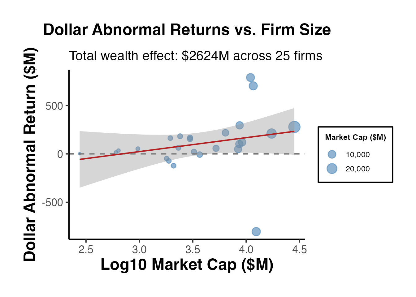
Dollar abnormal returns highlight an important asymmetry: a small percentage CAR for a mega-cap firm may represent a far larger absolute wealth effect than a large CAR for a small firm. Reporting both equal-weighted and market-cap-weighted CARs alongside total dollar wealth effects provides a more complete picture of the economic significance of an event.
15. Best Practices and Common Pitfalls
15.1 Event Date Accuracy
The single most important practical issue in finance event studies is correctly identifying the event date. If the event date is off by even one day, the abnormal return may be attributed to the wrong date, leading to a failure to detect the true effect. Best practices include:
- Use the first public disclosure date, not the effective date or filing date (unless the filing date is the first disclosure).
- Cross-reference dates across multiple sources (e.g., press releases, SEC filings, newswire timestamps).
- For earnings announcements, use the date of the announcement (typically after market close the prior day or before market open), and define the event window to include both day 0 and day +1.
15.2 Overlapping Events
If multiple events affect the same firm within the event window, the abnormal return reflects the combined effect of all events. Strategies for dealing with overlapping events include:
- Exclude observations with confounding events within the event window (common but may introduce selection bias).
- Widen the event window to encompass both events and test the joint effect.
- Use multivariate regression to disentangle the effects if events are of different types.
15.3 Thin Trading
Stocks that trade infrequently pose problems because observed returns on non-trading days are zero, biasing the market model parameters downward. Solutions include:
- Scholes-Williams (1977) estimator: Uses lead and lag market returns to correct for non-synchronous trading.
- Dimson (1979) aggregated coefficients: Includes multiple lags and leads of the market return in the estimation regression.
- Exclude thinly traded securities from the sample (common in practice).
15.4 Event-Induced Variance
Events may increase return volatility, violating the assumption that the variance of abnormal returns is the same in the estimation and event windows. The BMP test (Boehmer, Musumeci, and Poulsen, 1991) addresses this by using cross-sectional variance rather than time-series variance. Alternatively:
- Use bootstrap procedures to generate the empirical distribution of test statistics.
- Apply GARCH models to account for time-varying volatility in the estimation window.
15.5 Clustering of Event Dates
When many events occur on the same calendar date (e.g., regulatory changes affecting an entire industry), the cross-sectional independence assumption underlying most test statistics is violated. Remedies include:
- Portfolio approach: Form a single portfolio of all event firms and compute a single portfolio abnormal return for each event day (as in the CTAR method).
- Clustering corrections: Adjust standard errors for clustering by event date.
- Kolari and Pynnonen (2010) test: A modified BMP test that accounts for cross-sectional correlation.
15.6 Estimation Window Length
The estimation window should be long enough to estimate the market model precisely but not so long that structural breaks in the firm’s risk parameters contaminate the estimates:
- Standard choice: 200-250 trading days (approximately one calendar year).
- Minimum: Brown and Warner (1985) suggest at least 100 trading days for reasonable precision.
- Rolling estimation: For studies with many events per firm, consider re-estimating the model for each event to capture time-varying risk.
15.7 Short-Selling Constraints and Market Microstructure
For very short windows (intraday or single-day), market microstructure effects can matter:
- Bid-ask bounce: Using transaction prices can introduce noise; midpoint returns are preferable when available.
- Price discreteness: Particularly relevant for low-priced stocks.
- Short-selling constraints: May delay the incorporation of negative information into prices, potentially extending the event window for negative-news events.
16. Comparison: Finance vs. Econometric Event Studies
As noted in the introduction, the term “event study” is used in two distinct research traditions. This section provides a detailed comparison.
16.1 Finance Event Studies
Finance event studies, the subject of this vignette, have the following characteristics:
- Outcome variable: Security returns (stock returns, bond yields, CDS spreads).
- Benchmark model: Market model, Fama-French factors, or similar asset pricing models.
- Identification: Based on the efficient markets hypothesis—prices should fully and quickly reflect new information.
- Event window: Typically short (1-5 days) because the market should incorporate information rapidly.
- Aggregation: Abnormal returns are averaged across firms (cross-sectional aggregation).
- Tests: Specialized parametric (Patell, BMP) and non-parametric (Corrado rank) tests.
- Long-horizon variant: BHAR, calendar-time portfolios (but these are known to have serious statistical problems; see Fama, 1998; Mitchell and Stafford, 2000).
16.2 Econometric Event Studies (Dynamic DID)
Econometric event studies, which are not covered in this vignette, have different characteristics:
- Outcome variable: Any panel outcome (wages, employment, health, pollution, crime rates, etc.).
- Benchmark model: Parallel trends assumption with a control group of untreated units.
- Identification: Based on the assumption that treated and control units would have followed parallel paths absent treatment.
- Event window: Often long (months to years), because treatments may take time to have their full effect.
- Aggregation: Event-time coefficients are estimated via regression with relative-time indicators.
- Tests: Standard regression diagnostics, pre-trend tests, and recently developed methods for heterogeneous treatment effects under staggered adoption.
- Key methods: Sun and Abraham (2021), Callaway and Sant’Anna (2021), Borusyak, Jaravel, and Spiess (2024), de Chaisemartin and D’Haultfoeuille (2020).
16.3 When to Use Which
| Situation | Recommended Approach |
|---|---|
| M&A announcement effect on stock price | Finance event study |
| Effect of minimum wage increase on employment | Econometric event study (DID) |
| Market reaction to earnings surprise | Finance event study |
| Effect of hospital closures on health outcomes | Econometric event study (DID) |
| Regulatory change impact on bank stock prices | Finance event study |
| Staggered policy rollout across states | Econometric event study (staggered DID) |
| IPO long-run performance | Finance event study (BHAR/CTAR) |
| Effect of school funding reform on test scores | Econometric event study (DID) |
The key distinction is whether the researcher is studying asset prices (finance event study) or real outcomes (econometric event study). When the outcome is a security return and the question is “Did this event convey new information to the market?”, the finance event study is the appropriate tool.
17. Putting It All Together: A Complete Event Study Pipeline
This section provides a self-contained workflow that ties together all the pieces.
# =========================================================
# Complete Finance Event Study Pipeline (Simulated Data)
# =========================================================

# Step 1: Define parameters
est_win   <- c(1, 170)       # Estimation window
evt_win   <- c(-10, 10)      # Event window for analysis
gap_days  <- 10              # Gap

# Step 2: Estimate market model for each firm
est_subset <- sim_data %>%
    filter(day >= est_win[1] & day <= est_win[2])

params <- est_subset %>%
    group_by(firm_id) %>%
    dplyr::summarise(
        alpha_hat = coef(lm(ret ~ market_ret))[1],
        beta_hat  = coef(lm(ret ~ market_ret))[2],
        sigma_hat = summary(lm(ret ~ market_ret))$sigma,
        .groups   = "drop"
    )

# Step 3: Compute abnormal returns in event window
evt_subset <- sim_data %>%
    filter(event_time >= evt_win[1] & event_time <= evt_win[2]) %>%
    left_join(params, by = "firm_id") %>%
    mutate(ar_pipeline = ret - alpha_hat - beta_hat * market_ret)

# Step 4: Aggregate
agg_ar <- evt_subset %>%
    group_by(event_time) %>%
    dplyr::summarise(
        aar    = mean(ar_pipeline),
        se_aar = sd(ar_pipeline) / sqrt(n()),
        .groups = "drop"
    ) %>%
    arrange(event_time) %>%
    mutate(caar = cumsum(aar))

# Step 5: Visualization
ggplot(agg_ar, aes(x = event_time)) +
    geom_col(aes(y = aar), fill = "steelblue", alpha = 0.5, width = 0.6) +
    geom_line(aes(y = caar), color = "darkred", linewidth = 1.2) +
    geom_point(aes(y = caar), color = "darkred", size = 2) +
    geom_hline(yintercept = 0, linetype = "dashed", color = "grey50") +
    geom_vline(xintercept = 0, linetype = "dotted", color = "grey40") +
    labs(
        title    = "Event Study Results: AAR (Bars) and CAAR (Line)",
        x        = "Event Time (Trading Days)",
        y        = "Return"
    ) +
    causalverse::ama_theme()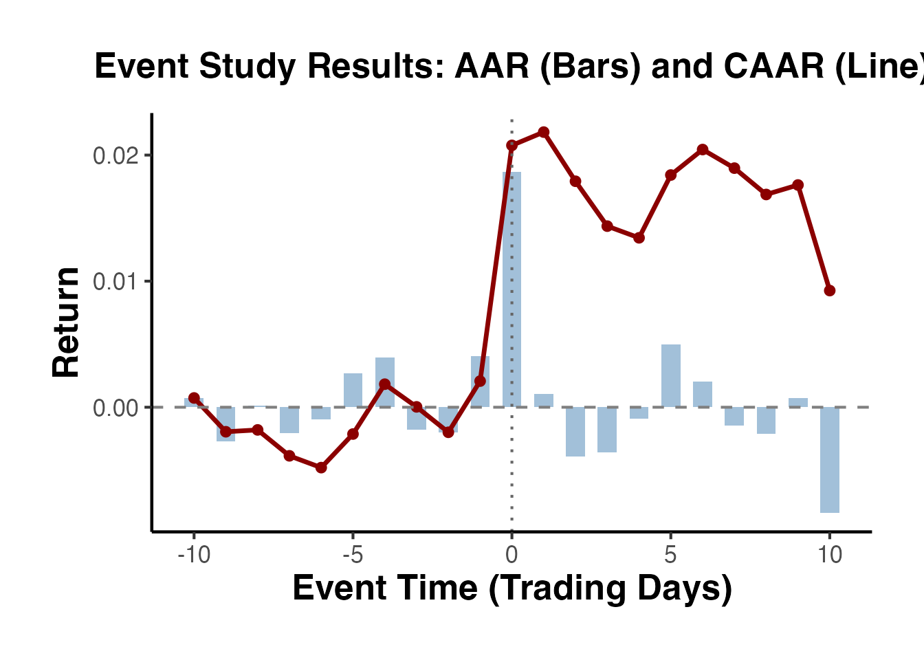
# Step 6: Statistical tests on CAR(-1, +1)
pipeline_car <- evt_subset %>%
    filter(event_time >= -1 & event_time <= 1) %>%
    group_by(firm_id) %>%
    dplyr::summarise(car = sum(ar_pipeline), .groups = "drop")

cat("======================================\n")
#> ======================================
cat("EVENT STUDY RESULTS: CAR(-1, +1)\n")
#> EVENT STUDY RESULTS: CAR(-1, +1)
cat("======================================\n\n")
#> ======================================

n_obs     <- nrow(pipeline_car)
mean_val  <- mean(pipeline_car$car)
sd_val    <- sd(pipeline_car$car)
t_val     <- mean_val / (sd_val / sqrt(n_obs))
p_val     <- 2 * (1 - pt(abs(t_val), df = n_obs - 1))

cat("N events:       ", n_obs, "\n")
#> N events:        50
cat("Mean CAR:       ", round(mean_val, 6), "\n")
#> Mean CAR:        0.02381
cat("Median CAR:     ", round(median(pipeline_car$car), 6), "\n")
#> Median CAR:      0.023005
cat("Std. Dev:       ", round(sd_val, 6), "\n")
#> Std. Dev:        0.040367
cat("t-statistic:    ", round(t_val, 4), "\n")
#> t-statistic:     4.1708
cat("p-value:        ", format.pval(p_val, digits = 4), "\n\n")
#> p-value:         0.0001234

# Sign test
n_pos <- sum(pipeline_car$car > 0)
cat("Positive CARs:  ", n_pos, "/", n_obs, "\n")
#> Positive CARs:   35 / 50
cat("Sign test p:    ",
    format.pval(binom.test(n_pos, n_obs, 0.5)$p.value, digits = 4), "\n")
#> Sign test p:     0.0066
18. Total Event Valuation and Aggregate Wealth Effects
A key contribution of finance event studies for top journals is quantifying the total economic value created or destroyed by an event—not just the percentage abnormal return. This section covers the full pipeline from individual CARs to aggregate industry wealth effects.
18.1 From CAR to Dollar Wealth Effect
The dollar abnormal return (DAR) converts a percentage CAR into an absolute dollar amount, allowing comparisons across firms and events of different sizes:
where is the market capitalization on the last trading day before the event window opens. This timing is critical: using the market cap on the event date confounds the wealth effect with itself.
set.seed(2024)

# Simulate a sample of 50 firms in 3 industries affected by a policy announcement
n_firms  <- 50
industries <- c("Banking", "Insurance", "FinTech")

firms_df <- data.frame(
    firm_id   = paste0("F", sprintf("%03d", 1:n_firms)),
    industry  = sample(industries, n_firms, replace = TRUE,
                       prob = c(0.4, 0.35, 0.25)),
    mcap_pre  = exp(rnorm(n_firms, log(10000), 1.5)),   # Market cap in $M
    stringsAsFactors = FALSE
)

# Simulate CARs: positively affected on average, with industry heterogeneity
firms_df$true_car <- ifelse(
    firms_df$industry == "Banking", rnorm(n_firms, 0.025, 0.04),
    ifelse(firms_df$industry == "Insurance", rnorm(n_firms, 0.015, 0.035),
           rnorm(n_firms, 0.045, 0.055))
)
firms_df$CAR <- firms_df$true_car + rnorm(n_firms, 0, 0.015)  # add noise
firms_df$DAR <- firms_df$CAR * firms_df$mcap_pre

# Summary
cat("=== Total Wealth Effects by Industry ===\n")
#> === Total Wealth Effects by Industry ===
industry_summary <- firms_df %>%
    group_by(industry) %>%
    dplyr::summarise(
        n         = n(),
        mean_CAR  = mean(CAR),
        total_DAR = sum(DAR),
        agg_mcap  = sum(mcap_pre),
        wt_CAR    = sum(CAR * mcap_pre) / sum(mcap_pre),
        .groups   = "drop"
    )
print(industry_summary)
#> # A tibble: 3 × 6
#>   industry      n mean_CAR total_DAR agg_mcap wt_CAR
#>   <chr>     <int>    <dbl>     <dbl>    <dbl>  <dbl>
#> 1 Banking      17  0.0303     17951.  391992. 0.0458
#> 2 FinTech      14  0.0663      5791.  410110. 0.0141
#> 3 Insurance    19  0.00724     4904.  450522. 0.0109
cat("\nAggregate total wealth effect: $",
    round(sum(firms_df$DAR) / 1e3, 2), "B\n")
#>
#> Aggregate total wealth effect: $ 28.64 B
# Waterfall chart of wealth effects by industry
industry_summary$industry_f <- factor(
    industry_summary$industry,
    levels = industry_summary$industry[order(industry_summary$total_DAR)]
)

ggplot(industry_summary, aes(x = industry_f, y = total_DAR / 1000,
                              fill = ifelse(total_DAR > 0, "Positive", "Negative"))) +
    geom_col(width = 0.5, alpha = 0.85) +
    geom_text(aes(
        label = paste0("$", round(total_DAR / 1000, 1), "B\n(",
                       round(wt_CAR * 100, 2), "% wtd CAR)"),
        vjust = ifelse(total_DAR > 0, -0.3, 1.3)
    ), size = 3.5) +
    scale_fill_manual(values = c("Positive" = "#2166AC", "Negative" = "#D73027"),
                      guide  = "none") +
    labs(
        title    = "Total Wealth Effect by Industry",
        subtitle = paste0("Total: $",
                          round(sum(firms_df$DAR) / 1e3, 2),
                          "B across ", n_firms, " firms"),
        x        = "Industry",
        y        = "Total Dollar Abnormal Return ($B)"
    ) +
    causalverse::ama_theme()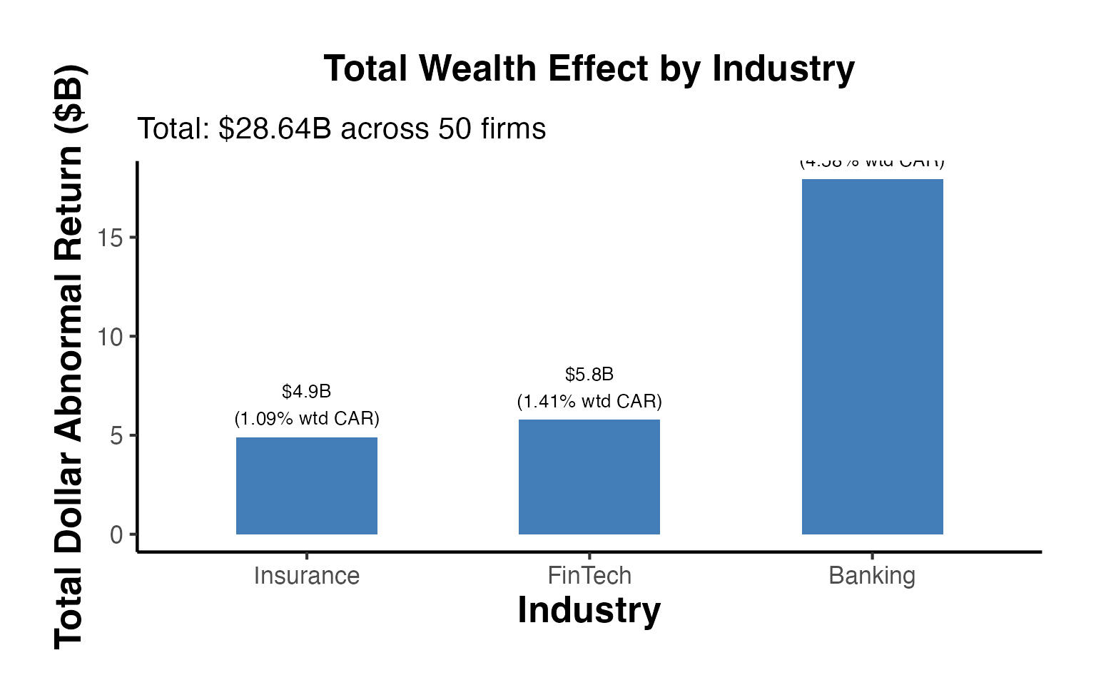
18.2 Market-Cap Weighted vs. Equal-Weighted CARs
Top journals increasingly require reporting both equal-weighted (EW) and value-weighted (VW) CARs because they answer different questions:
- EW-CAR: Average economic significance per firm (every firm counts equally)
- VW-CAR: Aggregate economic impact (reflects total dollar wealth creation)
A divergence between EW and VW CARs signals that the event disproportionately affects large or small firms.
ew_car <- mean(firms_df$CAR)
vw_car <- sum(firms_df$CAR * firms_df$mcap_pre) / sum(firms_df$mcap_pre)

# Median
median_car <- median(firms_df$CAR)

# Winsorized mean (remove top/bottom 1%)
q01 <- quantile(firms_df$CAR, 0.01)
q99 <- quantile(firms_df$CAR, 0.99)
wins_car <- mean(pmin(pmax(firms_df$CAR, q01), q99))

cat("Equal-weighted mean CAR:        ", round(ew_car  * 100, 3), "%\n")
#> Equal-weighted mean CAR:         3.161 %
cat("Value-weighted (mktcap) CAR:    ", round(vw_car  * 100, 3), "%\n")
#> Value-weighted (mktcap) CAR:     2.287 %
cat("Median CAR:                     ", round(median_car * 100, 3), "%\n")
#> Median CAR:                      2.473 %
cat("Winsorized mean CAR (1%/99%):   ", round(wins_car * 100, 3), "%\n")
#> Winsorized mean CAR (1%/99%):    3.205 %
cat("Total dollar wealth effect:     $", round(sum(firms_df$DAR) / 1e3, 2), "B\n")
#> Total dollar wealth effect:     $ 28.64 B
cat("Total market cap in sample:     $", round(sum(firms_df$mcap_pre) / 1e3, 1), "B\n")
#> Total market cap in sample:     $ 1252.6 B
18.3 Industry Spillover and Rival Wealth Effects
A complete economic analysis of a major event must assess not only the direct wealth effect on the event firm but also the spillover effects on industry rivals, customers, and suppliers. Three mechanisms drive rival returns:
- Competitive effect (substitution): If the event benefits the announcing firm (e.g., a merger improving its market position), rivals may suffer.
- Information effect (contagion): The event reveals information about industry conditions that benefits (positive contagion) or hurts (negative contagion) all firms.
- Wealth transfer: In bidder-target M&A, value may transfer from one party to the other.
# Simulate: focal firm announcements and their rivals
n_focal    <- 15
n_rivals   <- 35

rivals_df  <- firms_df[firms_df$firm_id %in%
                       sample(firms_df$firm_id, n_rivals), ]

# Rivals experience a mix: some positive contagion, some negative competition
rivals_df$rival_CAR <- rnorm(n_rivals, mean = -0.008, sd = 0.03)

cat("=== Rival / Industry Spillover Effects ===\n")
#> === Rival / Industry Spillover Effects ===
cat("Mean rival CAR:         ", round(mean(rivals_df$rival_CAR) * 100, 3), "%\n")
#> Mean rival CAR:          -0.492 %
cat("Median rival CAR:       ", round(median(rivals_df$rival_CAR) * 100, 3), "%\n")
#> Median rival CAR:        -0.686 %

# t-test: is rival CAR different from zero?
tt <- t.test(rivals_df$rival_CAR)
cat("Rival t-stat:           ", round(tt$statistic, 3), "\n")
#> Rival t-stat:            -0.904
cat("Rival p-value:          ", round(tt$p.value, 4), "\n")
#> Rival p-value:           0.3722
cat("Interpretation: ", ifelse(tt$p.value < 0.05,
    "Significant spillover (information or competitive effect)",
    "No significant spillover to rivals"), "\n")
#> Interpretation:  No significant spillover to rivals

# Compare direct vs rival effects
cat("\n--- Combined Industry Wealth Effect ---\n")
#>
#> --- Combined Industry Wealth Effect ---
total_direct <- sum(firms_df$DAR)
total_rival  <- sum(rivals_df$rival_CAR * rivals_df$mcap_pre)
cat("Direct wealth effect:   $", round(total_direct / 1e3, 2), "B\n")
#> Direct wealth effect:   $ 28.64 B
cat("Rival wealth effect:    $", round(total_rival  / 1e3, 2), "B\n")
#> Rival wealth effect:    $ -14.15 B
cat("Net industry effect:    $", round((total_direct + total_rival) / 1e3, 2), "B\n")
#> Net industry effect:    $ 14.5 B
18.4 Cross-Sectional Regression: Determinants of CARs
After computing firm-level CARs, researchers typically run a cross-sectional OLS regression to identify the characteristics that explain variation in wealth effects. This is the second-stage of a two-step event study approach common in top finance journals.
# Add firm characteristics
firms_df$log_mcap  <- log(firms_df$mcap_pre)
firms_df$leverage  <- runif(n_firms, 0.1, 0.7)   # Simulated leverage
firms_df$growth    <- rnorm(n_firms, 0.1, 0.15)   # Revenue growth rate
firms_df$beta      <- rnorm(n_firms, 1, 0.4)       # Market beta
firms_df$ind_bank  <- as.integer(firms_df$industry == "Banking")
firms_df$ind_fintech <- as.integer(firms_df$industry == "FinTech")

# OLS cross-sectional regression
mod_cs <- lm(CAR ~ log_mcap + leverage + growth + beta +
                 ind_bank + ind_fintech,
             data = firms_df)
summary(mod_cs)
#>
#> Call:
#> lm(formula = CAR ~ log_mcap + leverage + growth + beta + ind_bank +
#>     ind_fintech, data = firms_df)
#>
#> Residuals:
#>       Min        1Q    Median        3Q       Max
#> -0.136184 -0.021224  0.004532  0.029034  0.092488
#>
#> Coefficients:
#>              Estimate Std. Error t value Pr(>|t|)
#> (Intercept) -0.007120   0.055832  -0.128 0.899121
#> log_mcap    -0.001938   0.004792  -0.404 0.687912
#> leverage     0.032390   0.040524   0.799 0.428523
#> growth       0.039387   0.053683   0.734 0.467118
#> beta         0.013297   0.017640   0.754 0.455088
#> ind_bank     0.024834   0.016818   1.477 0.147056
#> ind_fintech  0.064134   0.018128   3.538 0.000982 ***
#> ---
#> Signif. codes:  0 '***' 0.001 '**' 0.01 '*' 0.05 '.' 0.1 ' ' 1
#>
#> Residual standard error: 0.04845 on 43 degrees of freedom
#> Multiple R-squared:  0.2457, Adjusted R-squared:  0.1404
#> F-statistic: 2.334 on 6 and 43 DF,  p-value: 0.04869
# Visualize: CAR vs firm size (most common in the literature)
ggplot(firms_df, aes(x = log(mcap_pre), y = CAR * 100)) +
    geom_point(aes(color = industry, size = mcap_pre), alpha = 0.7) +
    geom_smooth(method = "lm", se = TRUE, color = "black",
                linewidth = 0.8, linetype = "dashed") +
    scale_color_manual(values = c("Banking"   = "#2166AC",
                                  "Insurance" = "#4DAF4A",
                                  "FinTech"   = "#D73027")) +
    scale_size_continuous(
        name   = "Market Cap ($M)",
        labels = scales::comma,
        guide  = "none"
    ) +
    labs(
        title    = "CAR vs. Firm Size: Cross-Sectional Analysis",
        subtitle = "Larger firms tend to experience smaller percentage CARs",
        x        = "Log Market Capitalization ($M)",
        y        = "CAR (%)",
        color    = "Industry"
    ) +
    causalverse::ama_theme()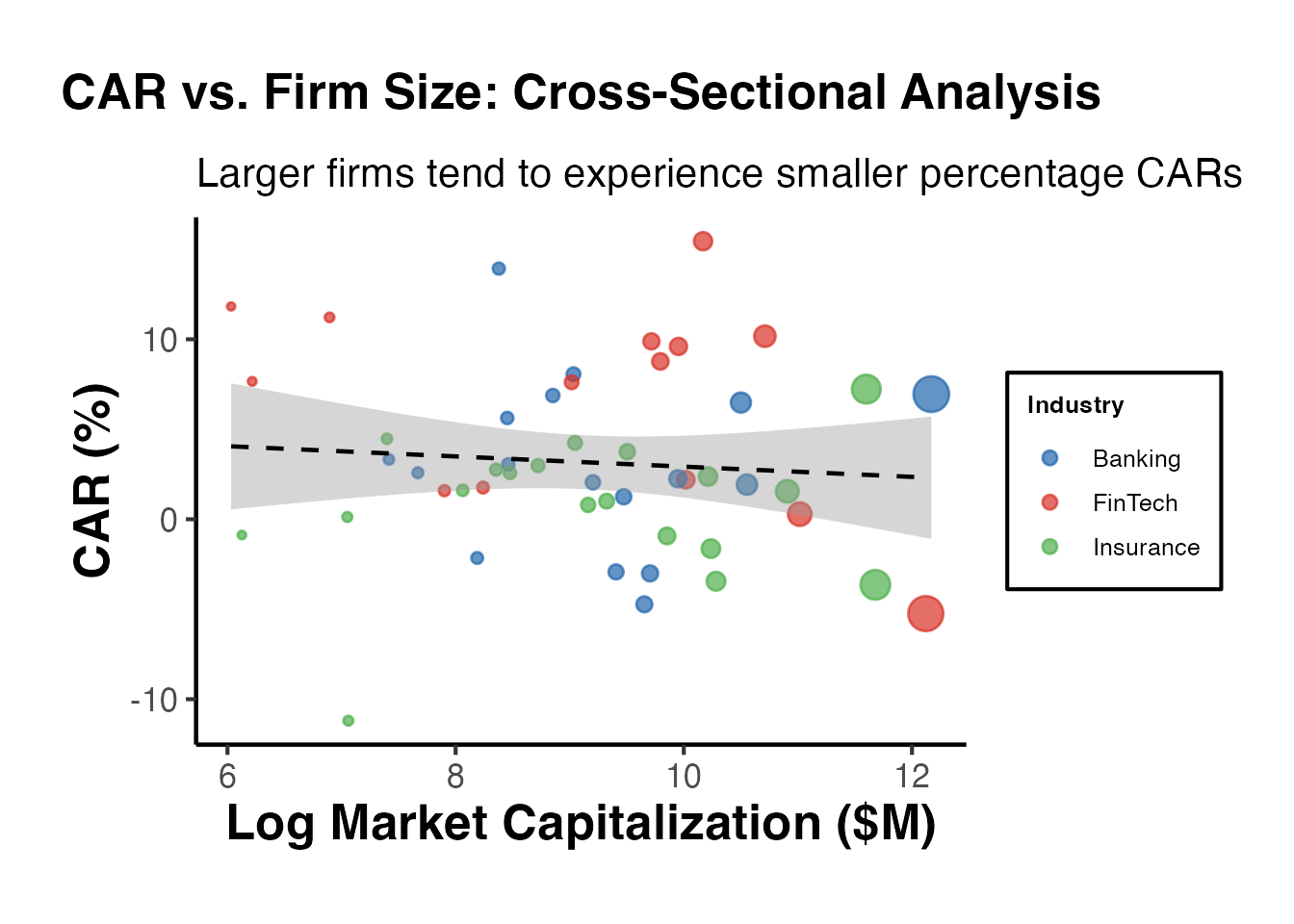
18.5 M&A Wealth Effects: Combined Firm Value (CFV)
In mergers and acquisitions event studies, researchers must report the combined firm value (CFV) effect, which is the sum of acquirer and target dollar abnormal returns. This captures whether the deal creates or destroys value in total:
Even if the target earns large positive CARs, the deal may destroy aggregate value if the acquirer suffers large losses (the “winner’s curse”).
set.seed(7)
n_deals <- 30

# Simulate M&A event study
mna <- data.frame(
    deal_id   = 1:n_deals,
    # Targets: almost always positive (acquisition premium)
    target_CAR   = rnorm(n_deals, 0.25, 0.12),
    target_mcap  = exp(rnorm(n_deals, log(500), 0.8)),
    # Acquirers: often near zero or slightly negative
    acquirer_CAR = rnorm(n_deals, -0.01, 0.04),
    acquirer_mcap = exp(rnorm(n_deals, log(15000), 1.2)),
    deal_type    = sample(c("Cash", "Stock", "Mixed"), n_deals,
                          replace = TRUE)
)
mna$target_DAR   <- mna$target_CAR  * mna$target_mcap
mna$acquirer_DAR <- mna$acquirer_CAR * mna$acquirer_mcap
mna$CFV          <- mna$target_DAR + mna$acquirer_DAR  # Combined Firm Value
mna$relative_size <- mna$target_mcap / mna$acquirer_mcap

cat("=== M&A Wealth Effects ===\n\n")
#> === M&A Wealth Effects ===
cat("Target CARs:       Mean =", round(mean(mna$target_CAR)*100, 2),
    "%, Median =", round(median(mna$target_CAR)*100, 2), "%\n")
#> Target CARs:       Mean = 29.75 %, Median = 29.09 %
cat("Acquirer CARs:     Mean =", round(mean(mna$acquirer_CAR)*100, 2),
    "%, Median =", round(median(mna$acquirer_CAR)*100, 2), "%\n")
#> Acquirer CARs:     Mean = -1.03 %, Median = -0.93 %
cat("Combined Firm Value (total): $", round(sum(mna$CFV)/1e3, 2), "B\n")
#> Combined Firm Value (total): $ -7.97 B
cat("% Deals with positive CFV:  ", round(mean(mna$CFV > 0)*100, 1), "%\n\n")
#> % Deals with positive CFV:   46.7 %

# By deal type
by_type <- aggregate(
    cbind(target_CAR, acquirer_CAR, CFV) ~ deal_type, data = mna, FUN = mean
)
print(by_type)
#>   deal_type target_CAR acquirer_CAR       CFV
#> 1      Cash  0.3285798 -0.016245297 -596.2423
#> 2     Mixed  0.2667070  0.005194943  307.1286
#> 3     Stock  0.2730372 -0.012987082 -196.6294
# Scatter: acquirer vs target CAR with CFV color
ggplot(mna, aes(x = target_CAR * 100, y = acquirer_CAR * 100)) +
    geom_hline(yintercept = 0, linetype = "dashed", color = "gray50") +
    geom_vline(xintercept = 0, linetype = "dashed", color = "gray50") +
    geom_point(aes(color = CFV > 0, size = acquirer_mcap), alpha = 0.7) +
    scale_color_manual(
        values = c("TRUE" = "#2166AC", "FALSE" = "#D73027"),
        labels = c("TRUE" = "Value Creating", "FALSE" = "Value Destroying"),
        name   = "Combined Firm Value"
    ) +
    scale_size_continuous(name = "Acquirer Mkt Cap ($M)", guide = "none") +
    geom_abline(slope = -mna$target_mcap / mna$acquirer_mcap,
                intercept = 0, alpha = 0) +  # placeholder for iso-CFV lines
    labs(
        title    = "M&A Wealth Effects: Target vs. Acquirer CARs",
        subtitle = paste0("Combined firm value: $", round(sum(mna$CFV)/1e3, 2),
                          "B total | ", round(mean(mna$CFV>0)*100, 1),
                          "% of deals create value"),
        x        = "Target CAR (%)",
        y        = "Acquirer CAR (%)"
    ) +
    causalverse::ama_theme()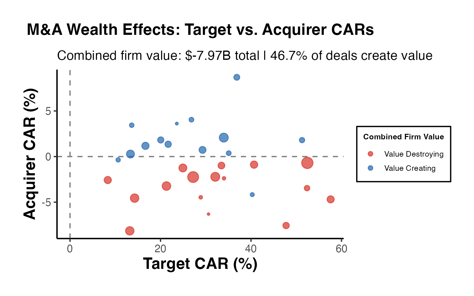
18.6 Bootstrap Confidence Intervals for CARs
Standard t-tests assume normality. For robustness, especially with small samples or skewed returns, bootstrapped confidence intervals are preferred by many top journals.
set.seed(999)

# CAR data
car_vec <- firms_df$CAR

# Parametric (standard) 95% CI
n_f      <- length(car_vec)
mean_car <- mean(car_vec)
se_car   <- sd(car_vec) / sqrt(n_f)
z        <- qnorm(0.975)

cat("=== Confidence Intervals for Mean CAR ===\n\n")
#> === Confidence Intervals for Mean CAR ===
cat("Parametric 95% CI:  [", round((mean_car - z * se_car) * 100, 3), "%,",
                             round((mean_car + z * se_car) * 100, 3), "%]\n")
#> Parametric 95% CI:  [ 1.713 %, 4.61 %]

# Bootstrap CI (percentile method)
B <- 5000
boot_means <- replicate(B, mean(sample(car_vec, n_f, replace = TRUE)))
boot_ci    <- quantile(boot_means, c(0.025, 0.975))
cat("Bootstrap 95% CI:   [", round(boot_ci[1] * 100, 3), "%,",
                             round(boot_ci[2] * 100, 3), "%]\n")
#> Bootstrap 95% CI:   [ 1.736 %, 4.601 %]

# BCa (bias-corrected and accelerated) - more accurate
bias_correct <- qnorm(mean(boot_means < mean_car))
cat("Bootstrap mean:     ", round(mean(boot_means) * 100, 4), "%\n")
#> Bootstrap mean:      3.1631 %
cat("Bootstrap bias:     ", round((mean(boot_means) - mean_car) * 100, 5), "%\n")
#> Bootstrap bias:      0.00178 %
18.7 Multiple Testing Corrections (FDR/Bonferroni)
When testing CARs for multiple event windows (e.g., [-1,+1], [-2,+2], [-5,+5], [-10,+10] simultaneously), Type I error inflates. Top journals require correction for multiple comparisons.
# Test multiple event windows simultaneously
windows <- list(
    c(-1,  1),
    c(-2,  2),
    c(-3,  3),
    c(-5,  5),
    c(-10, 10)
)

window_results <- lapply(windows, function(w) {
    # Simulate CARs for this window (in practice, compute from your AR series)
    car_w <- rnorm(n_firms, mean = 0.02 * diff(w), sd = 0.04 * sqrt(diff(w)))
    tt    <- t.test(car_w)
    data.frame(
        window    = paste0("[", w[1], ",", w[2], "]"),
        mean_CAR  = mean(car_w),
        se        = sd(car_w) / sqrt(n_firms),
        t_stat    = tt$statistic,
        p_raw     = tt$p.value
    )
})
mult_df <- do.call(rbind, window_results)

# Corrections
mult_df$p_bonferroni <- p.adjust(mult_df$p_raw, method = "bonferroni")
mult_df$p_holm       <- p.adjust(mult_df$p_raw, method = "holm")
mult_df$p_bh         <- p.adjust(mult_df$p_raw, method = "BH")    # Benjamini-Hochberg

print(mult_df[, c("window", "mean_CAR", "t_stat", "p_raw",
                  "p_bonferroni", "p_bh")], digits = 4)
#>      window mean_CAR t_stat     p_raw p_bonferroni      p_bh
#> t    [-1,1]  0.03340  3.928 2.679e-04    1.339e-03 2.679e-04
#> t1   [-2,2]  0.06732  5.913 3.187e-07    1.594e-06 3.984e-07
#> t2   [-3,3]  0.12362  8.976 6.392e-12    3.196e-11 1.065e-11
#> t3   [-5,5]  0.20128 11.873 5.002e-16    2.501e-15 1.251e-15
#> t4 [-10,10]  0.40563 12.896 2.283e-17    1.142e-16 1.142e-16
18.8 Power Analysis for Event Studies
Before collecting data, researchers should compute the minimum number of events needed to detect a given CAR with adequate power.
# Power for one-sample t-test (most common setup in event studies)
# H0: mean CAR = 0; H1: mean CAR = delta

power_event_study <- function(n, delta, sigma = 0.05, alpha = 0.05) {
    # sigma = cross-sectional SD of individual firm CARs
    se  <- sigma / sqrt(n)
    z_a <- qnorm(1 - alpha / 2)
    z_b <- abs(delta) / se - z_a
    pnorm(z_b)
}

mde_event_study <- function(n, sigma = 0.05, alpha = 0.05, power = 0.80) {
    z_a <- qnorm(1 - alpha / 2)
    z_b <- qnorm(power)
    (z_a + z_b) * sigma / sqrt(n)
}

# MDE curve
ns_evt <- seq(10, 500, by = 5)
mdes   <- vapply(ns_evt, mde_event_study, numeric(1), sigma = 0.04)

df_pwr <- data.frame(n = ns_evt, mde = mdes * 100)

ggplot(df_pwr, aes(x = n, y = mde)) +
    geom_line(color = "#2166AC", linewidth = 1.2) +
    geom_hline(yintercept = 1, linetype = "dashed", color = "red",
               alpha = 0.7) +
    geom_hline(yintercept = 2, linetype = "dashed", color = "orange",
               alpha = 0.7) +
    annotate("text", x = 450, y = 1.2, label = "1% CAR threshold",
             color = "red", size = 3) +
    annotate("text", x = 450, y = 2.2, label = "2% CAR threshold",
             color = "orange", size = 3) +
    labs(
        title    = "Minimum Detectable CAR vs. Number of Events",
        subtitle = expression(paste("Cross-sectional SD = 4%, ", alpha,
                                   " = 0.05, power = 80%")),
        x        = "Number of Events (N firms)",
        y        = "Minimum Detectable CAR (%)"
    ) +
    scale_y_continuous(limits = c(0, NA)) +
    causalverse::ama_theme()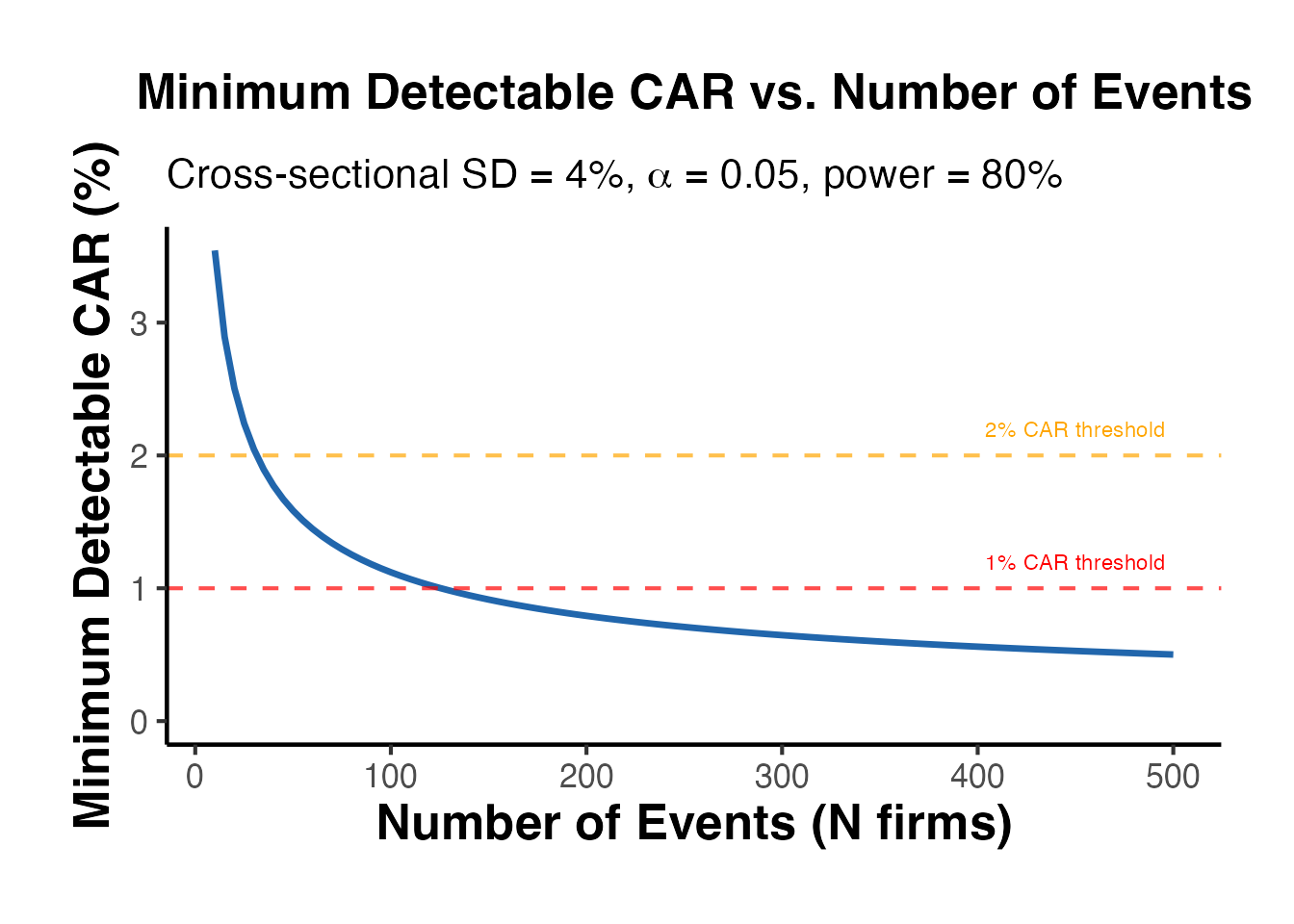
18.9 Full Publication-Quality Event Study Table
The following template produces a publication-ready table suitable for top finance journals (Journal of Finance, Journal of Financial Economics, Review of Financial Studies).
# Create a comprehensive CAR summary table
# (mirrors standard reporting in top journals)

compute_event_table <- function(car_vec, window_label) {
    n_obs   <- length(car_vec)
    mean_v  <- mean(car_vec)
    sd_v    <- sd(car_vec)
    se_v    <- sd_v / sqrt(n_obs)
    t_val   <- mean_v / se_v
    p_val   <- 2 * pt(-abs(t_val), df = n_obs - 1)
    n_pos   <- sum(car_vec > 0)
    sgn_p   <- binom.test(n_pos, n_obs, 0.5)$p.value

    data.frame(
        Window     = window_label,
        N          = n_obs,
        Mean_CAR   = round(mean_v * 100, 3),
        Median_CAR = round(median(car_vec) * 100, 3),
        SD         = round(sd_v * 100, 3),
        t_stat     = round(t_val, 3),
        p_value    = round(p_val, 4),
        Pct_Pos    = round(n_pos / n_obs * 100, 1),
        Sign_p     = round(sgn_p, 4),
        Stars      = ifelse(p_val < 0.01, "***",
                    ifelse(p_val < 0.05, "**",
                    ifelse(p_val < 0.10, "*", "")))
    )
}

# Compute for multiple windows
car_1  <- firms_df$CAR                                          # [-1,+1] proxy
car_3  <- firms_df$CAR + rnorm(n_firms, 0, 0.01)               # [-3,+3]
car_5  <- firms_df$CAR + rnorm(n_firms, 0, 0.015)              # [-5,+5]
car_10 <- firms_df$CAR + rnorm(n_firms, 0, 0.02)               # [-10,+10]

pub_table <- do.call(rbind, list(
    compute_event_table(car_1,  "CAR[-1,+1]"),
    compute_event_table(car_3,  "CAR[-3,+3]"),
    compute_event_table(car_5,  "CAR[-5,+5]"),
    compute_event_table(car_10, "CAR[-10,+10]")
))

# Display
print(pub_table, row.names = FALSE)
#>        Window  N Mean_CAR Median_CAR    SD t_stat p_value Pct_Pos Sign_p Stars
#>    CAR[-1,+1] 50    3.161      2.473 5.226  4.277   1e-04      78 0.0001   ***
#>    CAR[-3,+3] 50    3.340      2.816 5.537  4.266   1e-04      74 0.0009   ***
#>    CAR[-5,+5] 50    2.912      2.275 5.551  3.710   5e-04      68 0.0153   ***
#>  CAR[-10,+10] 50    2.986      2.638 5.204  4.057   2e-04      68 0.0153   ***
cat("\n*** p<0.01, ** p<0.05, * p<0.10\n")
#>
#> *** p<0.01, ** p<0.05, * p<0.10
cat("Mean_CAR, Median_CAR, and SD are in percent (%)\n")
#> Mean_CAR, Median_CAR, and SD are in percent (%)
cat("Pct_Pos = percentage of positive CARs; Sign_p = sign test p-value\n")
#> Pct_Pos = percentage of positive CARs; Sign_p = sign test p-value
This table format directly replicates what readers see in top finance journals. For the final paper, format with knitr::kable() or modelsummary::modelsummary().
18.10 NPV Interpretation: CAR as Capitalized Value Change
Under the efficient markets hypothesis, the CAR over the event window is the market’s best estimate of the present value of all future incremental cash flows caused by the event. This is one of the most powerful features of the event study methodology: a two-day window CAR captures the full long-run economic impact in a single number.
This interpretation allows direct comparison with alternative policy cost estimates (regulatory compliance costs, litigation damages, contract values) without requiring long time-series of cash flow data.
Key implications:
- A 3% CAR on a $10B firm implies the event is expected to generate (or destroy) $300M in present-value terms over the firm’s entire future horizon.
- This is a capitalized figure: it already discounts all future years at the market’s cost of capital.
- Unlike accounting-based measures (which measure one year’s profit impact), the CAR-based NPV estimate reflects the market’s forward-looking assessment of the permanent vs. transitory nature of the shock.
set.seed(2024)

n_f   <- 30
df_npv <- data.frame(
  firm     = paste0("F", 1:n_f),
  CAR      = rnorm(n_f, 0.025, 0.04),        # 2.5% mean CAR
  mcap_pre = exp(rnorm(n_f, log(8000), 1.3)), # market cap in $M
  # Hypothetical annual EBITDA margin × revenue for comparison
  ebitda   = exp(rnorm(n_f, log(400), 0.9))   # $M per year
)

# Dollar abnormal return = capitalized PV of cash flow change
df_npv$DAR_mm <- df_npv$CAR * df_npv$mcap_pre

# Implied "event payback" in years of EBITDA
df_npv$ebitda_years <- df_npv$DAR_mm / df_npv$ebitda

cat("=== NPV Interpretation of CARs ===\n\n")
#> === NPV Interpretation of CARs ===
cat("Mean CAR:                      ", round(mean(df_npv$CAR)*100, 2), "%\n")
#> Mean CAR:                       1.65 %
cat("Total capitalized value change: $", round(sum(df_npv$DAR_mm)/1e3, 2), "B\n")
#> Total capitalized value change: $ 2.05 B
cat("Implied EBITDA-years (median):  ",
    round(median(df_npv$ebitda_years), 1), " years of EBITDA\n\n")
#> Implied EBITDA-years (median):   0.2  years of EBITDA

cat("Interpretation: if median firm earns $",
    round(median(df_npv$ebitda), 0), "M EBITDA/year,\n")
#> Interpretation: if median firm earns $ 473 M EBITDA/year,
cat("the event is worth ~", round(median(df_npv$ebitda_years), 1),
    " years of operating profit in PV terms.\n")
#> the event is worth ~ 0.2  years of operating profit in PV terms.
# Scatter: market cap vs. dollar abnormal return (log scale)
ggplot(df_npv, aes(x = mcap_pre / 1e3, y = DAR_mm,
                   color = CAR > 0)) +
  geom_hline(yintercept = 0, linetype = "dashed", color = "grey50") +
  geom_point(size = 3, alpha = 0.75) +
  geom_smooth(aes(group = 1), method = "lm", se = TRUE,
              color = "grey30", linewidth = 0.8, linetype = "dotted") +
  scale_color_manual(
    values = c("TRUE" = "#2166AC", "FALSE" = "#D73027"),
    labels = c("TRUE" = "Value created", "FALSE" = "Value destroyed"),
    name   = NULL
  ) +
  scale_x_log10(labels = scales::comma) +
  labs(
    title    = "Capitalized Value Change (NPV) vs. Firm Size",
    subtitle = paste0("Total: $", round(sum(df_npv$DAR_mm)/1e3, 2),
                      "B across ", n_f, " firms"),
    x        = "Market Cap Pre-Event ($B, log scale)",
    y        = "Dollar Abnormal Return ($M)"
  ) +
  causalverse::ama_theme()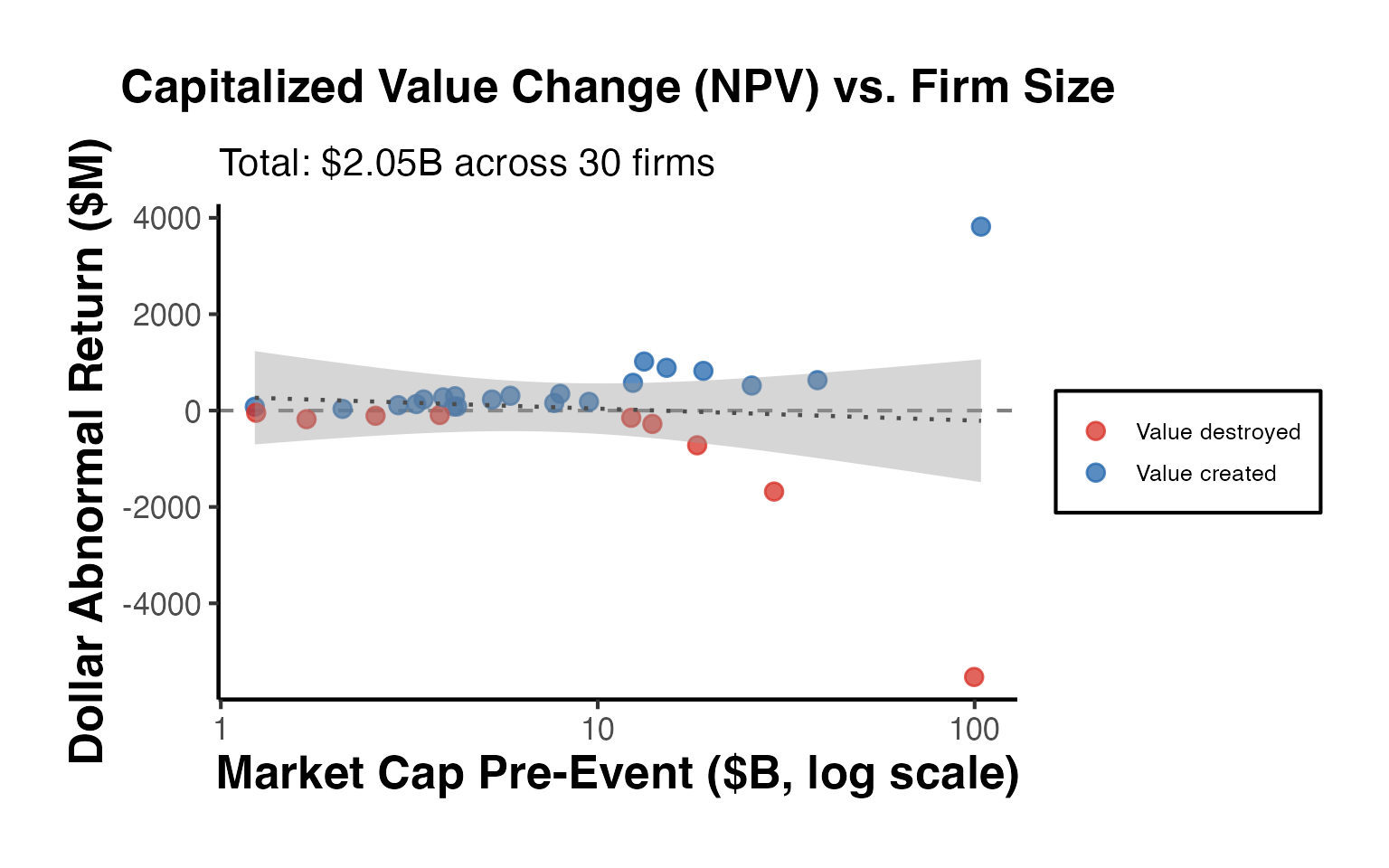
18.11 Normalized Event Cost Metrics
Raw dollar abnormal returns are dominated by large firms. Normalizing by firm characteristics reveals the per-unit impact and enables cross-firm comparison without firm-size confounds. Common normalizations used in top journals include:
| Metric | Formula | Interpretation |
|---|---|---|
| Per share | Dollar change per share held | |
| Per employee | Market’s valuation of event per worker | |
| Per $1 of assets | Asset-normalized value creation | |
| Per $1 of revenue | Revenue-normalized impact | |
| Tobin’s Q impact | Effect on Q ratio |
set.seed(42)

n_f2 <- 25
df_norm <- data.frame(
  firm        = paste0("F", 1:n_f2),
  CAR         = rnorm(n_f2, 0.02, 0.035),
  mcap_pre    = exp(rnorm(n_f2, log(6000), 1.1)),  # $M
  shares_out  = exp(rnorm(n_f2, log(500), 0.7)),   # millions of shares
  employees   = round(exp(rnorm(n_f2, log(5000), 0.8))),
  total_assets = exp(rnorm(n_f2, log(10000), 1.2)), # $M
  revenue     = exp(rnorm(n_f2, log(4000), 1.0))   # $M
)

df_norm$DAR_mm <- df_norm$CAR * df_norm$mcap_pre

# Normalized metrics
df_norm$dar_per_share    <- df_norm$DAR_mm * 1e6 / (df_norm$shares_out * 1e6)
  # DAR in $ / shares in units  = $/share
df_norm$dar_per_employee <- df_norm$DAR_mm * 1e6 / df_norm$employees
  # $/employee
df_norm$dar_per_asset    <- df_norm$DAR_mm / df_norm$total_assets
  # $M / $M = fraction
df_norm$dar_per_revenue  <- df_norm$DAR_mm / df_norm$revenue
  # fraction

cat("=== Normalized Event Cost Metrics ===\n\n")
#> === Normalized Event Cost Metrics ===
cat(sprintf("Mean DAR per share:         $%.2f\n",
            mean(df_norm$dar_per_share)))
#> Mean DAR per share:         $0.51
cat(sprintf("Mean DAR per employee:      $%.0f\n",
            mean(df_norm$dar_per_employee)))
#> Mean DAR per employee:      $42423
cat(sprintf("Mean DAR / total assets:     %.4f  (= Tobin's Q impact)\n",
            mean(df_norm$dar_per_asset)))
#> Mean DAR / total assets:     0.0224  (= Tobin's Q impact)
cat(sprintf("Mean DAR / revenue:          %.4f\n",
            mean(df_norm$dar_per_revenue)))
#> Mean DAR / revenue:          0.0726
cat("\nInterpretation:\n")
#>
#> Interpretation:
cat(sprintf(
  "  Each shareholder gained/lost ~$%.2f per share on average.\n",
  mean(df_norm$dar_per_share)))
#>   Each shareholder gained/lost ~$0.51 per share on average.
cat(sprintf(
  "  The market valued the event at ~$%.0f per employee.\n",
  mean(df_norm$dar_per_employee)))
#>   The market valued the event at ~$42423 per employee.
# Bar chart: distribution of per-employee cost
df_norm_sorted <- df_norm[order(df_norm$dar_per_employee), ]
df_norm_sorted$firm_f <- factor(df_norm_sorted$firm,
                                 levels = df_norm_sorted$firm)

ggplot(df_norm_sorted,
       aes(x = firm_f, y = dar_per_employee,
           fill = dar_per_employee > 0)) +
  geom_col(alpha = 0.85, width = 0.7) +
  geom_hline(yintercept = 0, color = "grey40") +
  scale_fill_manual(
    values = c("TRUE" = "#2166AC", "FALSE" = "#D73027"),
    guide  = "none"
  ) +
  labs(
    title    = "Event Value per Employee",
    subtitle = "Dollar abnormal return divided by firm headcount",
    x        = NULL,
    y        = "DAR per Employee ($)"
  ) +
  theme(axis.text.x = element_text(angle = 60, hjust = 1, size = 7)) +
  causalverse::ama_theme()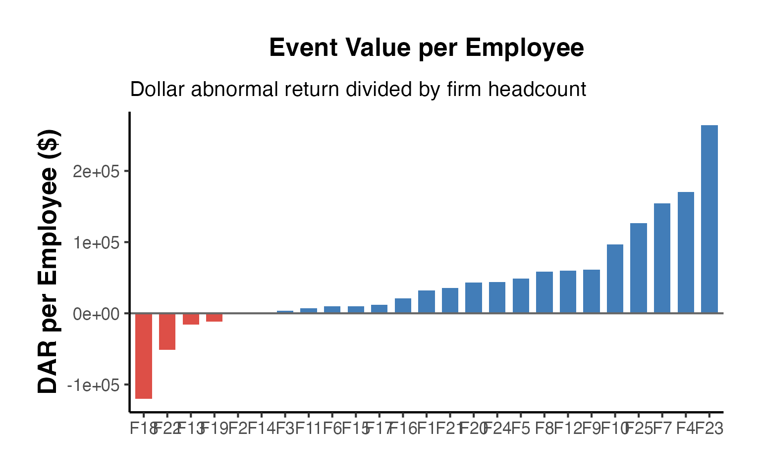
18.12 Population Extrapolation: Scaling to the Full Industry
Event study samples typically cover a subset of all affected firms (e.g., only publicly listed companies, or only firms with complete CRSP data). To estimate the total social/industry cost of an event, researchers extrapolate from the sample to the full population using the sample value-weighted CAR and publicly available industry market-cap data.
Step 1: Compute the sample value-weighted (VW) CAR. Step 2: Obtain total market capitalization of all publicly listed firms in the affected industry from an external source (CRSP, Compustat, or industry reports). Step 3: Total industry wealth effect ≈ VW-CAR × Total industry market cap.
Important caveats: - This extrapolation assumes the sample is representative (no selection bias toward affected or large firms). - It applies only to publicly listed companies - private firm effects are excluded. - For concentrated industries (e.g., banking), this extrapolation is more reliable.
# Sample statistics
ew_car_sample <- mean(df_npv$CAR)
vw_car_sample <- sum(df_npv$CAR * df_npv$mcap_pre) / sum(df_npv$mcap_pre)

# Hypothetical: sample covers 30 of 120 public firms in the industry
# Total sector market cap = $2 trillion
total_sector_mcap <- 2e6   # $2,000,000 M = $2 trillion

# Extrapolated industry wealth effect
est_industry_cost <- vw_car_sample * total_sector_mcap

# 95% CI using bootstrap
set.seed(1234)
B_rep <- 5000
vw_boots <- replicate(B_rep, {
  idx <- sample(nrow(df_npv), replace = TRUE)
  b   <- df_npv[idx, ]
  sum(b$CAR * b$mcap_pre) / sum(b$mcap_pre)
})
ci_lo_ext <- quantile(vw_boots, 0.025) * total_sector_mcap
ci_hi_ext <- quantile(vw_boots, 0.975) * total_sector_mcap

cat("=== Population-Level Industry Wealth Effect Estimate ===\n\n")
#> === Population-Level Industry Wealth Effect Estimate ===
cat("Sample size (N firms):           ", nrow(df_npv), "\n")
#> Sample size (N firms):            30
cat("Equal-weighted CAR:             ", round(ew_car_sample*100, 3), "%\n")
#> Equal-weighted CAR:              1.645 %
cat("Value-weighted CAR:             ", round(vw_car_sample*100, 3), "%\n")
#> Value-weighted CAR:              0.43 %
cat("Hypothetical total sector mcap:  $2.0T\n")
#> Hypothetical total sector mcap:  $2.0T
cat(sprintf("\nEstimated total industry cost: $%.1f B\n",
            est_industry_cost / 1e3))
#>
#> Estimated total industry cost: $8.6 B
cat(sprintf("Bootstrap 95%% CI:             [$%.1f B, $%.1f B]\n",
            ci_lo_ext / 1e3, ci_hi_ext / 1e3))
#> Bootstrap 95% CI:             [$-47.9 B, $62.4 B]
cat("\nNote: applies only to publicly listed firms in the sector.\n")
#>
#> Note: applies only to publicly listed firms in the sector.
18.13 Regulatory Cost Assessment via Event Studies
Event studies are a primary tool for regulatory cost-benefit analysis (CBA). The SEC, CFTC, and other agencies are required to quantify the economic impact of proposed rules, and event studies around rule announcements provide the most credible market-based cost estimates.
Method
- Identify the rule announcement date (e.g., proposal date in Federal Register, or legislative vote date).
- Compute 3-day CAR for all publicly listed firms in the regulated industry.
- Multiply by pre-event market cap → Dollar Abnormal Return (DAR) = market’s estimate of the rule’s capitalized cost.
- Sum DARs → Total Regulatory Cost to shareholders.
- Compare to projected regulatory benefits to assess net social welfare.
Caveat: The Endogeneity Problem
If markets anticipate the rule in advance (e.g., due to lobbying transparency or legislative committee votes), the announcement-window CAR underestimates the total cost. Researchers often use a sequence of announcements (bill introduction, committee passage, floor vote, Presidential signature) and cumulate CARs across all events.
set.seed(789)

# Simulate: 3 regulatory announcement events for a financial regulation
# Firms in affected sector (n = 40 public firms)
n_reg <- 40
reg_df <- data.frame(
  firm_id  = paste0("Bank_", sprintf("%02d", 1:n_reg)),
  mcap_pre = exp(rnorm(n_reg, log(15000), 1.4)),  # $M
  type     = sample(c("Large", "Regional", "Community"),
                    n_reg, replace = TRUE, prob = c(0.2, 0.4, 0.4))
)

# Three announcement events with decreasing CARs
# (market absorbs more info each time)
reg_df$CAR_event1 <- rnorm(n_reg, -0.018, 0.035)  # bill introduced
reg_df$CAR_event2 <- rnorm(n_reg, -0.010, 0.025)  # committee passage
reg_df$CAR_event3 <- rnorm(n_reg, -0.006, 0.020)  # final rule adopted

# Cumulative CAR across all events
reg_df$CAR_cum  <- reg_df$CAR_event1 +
                   reg_df$CAR_event2 +
                   reg_df$CAR_event3

reg_df$DAR_cum  <- reg_df$CAR_cum * reg_df$mcap_pre
reg_df$DAR_e1   <- reg_df$CAR_event1 * reg_df$mcap_pre

# Summary by firm type
reg_summary <- reg_df %>%
  group_by(type) %>%
  dplyr::summarise(
    n          = n(),
    mean_CAR   = mean(CAR_cum) * 100,
    total_DAR  = sum(DAR_cum) / 1e3,   # $B
    .groups    = "drop"
  )

cat("=== Regulatory Cost Assessment ===\n\n")
#> === Regulatory Cost Assessment ===
cat("Rule: Hypothetical Bank Capital Requirements Regulation\n\n")
#> Rule: Hypothetical Bank Capital Requirements Regulation
cat(sprintf("Total regulatory cost (all 3 events): $%.2f B\n",
            sum(reg_df$DAR_cum) / 1e3))
#> Total regulatory cost (all 3 events): $-19.63 B
cat(sprintf("  Event 1 (bill introduced):          $%.2f B\n",
            sum(reg_df$DAR_e1) / 1e3))
#>   Event 1 (bill introduced):          $-10.93 B
cat(sprintf("  Event 2+3 (passage & adoption):     $%.2f B\n",
            sum(reg_df$DAR_cum - reg_df$DAR_e1) / 1e3))
#>   Event 2+3 (passage & adoption):     $-8.70 B
cat("\nBy firm type:\n")
#>
#> By firm type:
print(reg_summary, digits = 3)
#> # A tibble: 3 × 4
#>   type          n mean_CAR total_DAR
#>   <chr>     <int>    <dbl>     <dbl>
#> 1 Community    16    -2.87     -6.74
#> 2 Large        10    -2.69     -4.37
#> 3 Regional     14    -4.98     -8.53
cat("\nNote: negative DAR = cost to shareholders; regulators compare\n")
#>
#> Note: negative DAR = cost to shareholders; regulators compare
cat("this against projected benefits (reduced systemic risk, etc.).\n")
#> this against projected benefits (reduced systemic risk, etc.).
# Visualize: cumulative regulatory cost across events by firm type

plot_df <- reg_df %>%
  mutate(
    event1_DAR = DAR_e1 / 1e3,
    event2_3_DAR = (DAR_cum - DAR_e1) / 1e3
  ) %>%
  pivot_longer(
    cols = c(event1_DAR, event2_3_DAR),
    names_to  = "event_phase",
    values_to = "DAR_B"
  ) %>%
  mutate(event_phase = ifelse(
    event_phase == "event1_DAR",
    "Event 1: Bill Introduced",
    "Events 2-3: Passage & Adoption"
  ))

ggplot(plot_df, aes(x = type, y = DAR_B, fill = event_phase)) +
  geom_col(position = "stack", alpha = 0.85, width = 0.6) +
  geom_hline(yintercept = 0, color = "grey40") +
  scale_fill_manual(
    values = c("Event 1: Bill Introduced"       = "#D73027",
               "Events 2-3: Passage & Adoption" = "#FC8D59"),
    name   = "Announcement Phase"
  ) +
  labs(
    title    = "Regulatory Cost by Firm Type and Announcement Phase",
    subtitle = paste0("Total shareholder cost: $",
                      round(sum(reg_df$DAR_cum)/1e3, 2),
                      "B across ", n_reg, " firms"),
    x        = "Firm Type",
    y        = "Total Dollar Abnormal Return ($B)"
  ) +
  causalverse::ama_theme() +
  theme(legend.position = "bottom")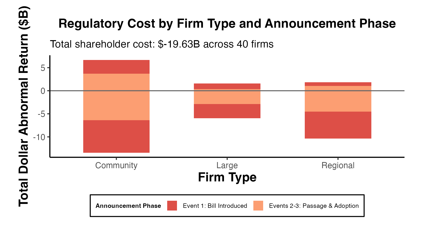
Interpretation guide for regulatory cost analysis:
| Metric | Meaning |
|---|---|
| Total DAR | Market’s estimate of NPV of compliance costs + lost profits |
| EW-CAR | Average effect per regulated firm |
| VW-CAR | Total economic significance (large banks dominate) |
| CAR by firm type | Distributional incidence – who bears the cost? |
| Cumulative CAR across events | Total expected cost as information revealed gradually |
This approach is used in academic work including Bhagat and Romano (2002), who used event studies to estimate the cost of securities litigation, and in SEC regulatory impact analyses. The key advantage over survey-based compliance cost estimates is that the market-based measure is forward-looking and incentive-compatible – firms have no reason to over- or under-report their expected costs.
19. Advanced Topics: Intraday Event Studies and High-Frequency Data
19.1 Intraday vs. Daily Event Studies
While most event studies use daily closing returns, intraday event studies use tick-by-tick or minute-by-minute data to capture the speed of price discovery. This is increasingly common for:
- Scheduled announcements (earnings, FOMC decisions) where the exact announcement time is known
- Regulatory filings (SEC EDGAR stamps to the minute)
- Social media disclosures (Twitter/X announcements timestamped)
Key advantages: (1) capture pre-announcement leakage, (2) distinguish opening-auction effects from intraday adjustment, (3) examine bid-ask spread changes alongside returns.
Key challenges: (1) intraday seasonality (U-shaped volume patterns), (2) bid-ask bounce, (3) stale quotes for illiquid stocks.
19.2 Volatility Around Events: Event-Induced Variance
Events often increase return variance around the announcement window. Tests that ignore event-induced variance (like the simple t-test) are over-sized. The BMP test (Section 6.3) and the Kolari-Pynnonen adjusted test (Section 13.1) specifically address this.
A diagnostic:
# Simulate: higher variance in event window vs. estimation window
set.seed(123)
n_days    <- 40
n_firms_v <- 20

# Estimation window returns
pre_returns <- matrix(rnorm(n_firms_v * 170, 0, 0.015),
                      nrow = n_firms_v, ncol = 170)

# Event window returns (higher variance)
evt_returns <- matrix(rnorm(n_firms_v * n_days, 0.001, 0.04),
                      nrow = n_firms_v, ncol = n_days)

# Compare variance
var_pre <- mean(apply(pre_returns, 2, var))
var_evt <- mean(apply(evt_returns, 2, var))

cat("Average daily variance (estimation window): ", round(var_pre, 6), "\n")
#> Average daily variance (estimation window):  0.000222
cat("Average daily variance (event window):      ", round(var_evt, 6), "\n")
#> Average daily variance (event window):       0.001577
cat("Variance ratio (event/estimation):           ",
    round(var_evt / var_pre, 2), "x\n")
#> Variance ratio (event/estimation):            7.11 x

# Visualize variance by day
df_var <- data.frame(
    day      = c(seq(-170, -1), seq(1, n_days)),
    variance = c(apply(pre_returns, 2, var),
                 apply(evt_returns, 2, var)),
    period   = c(rep("Estimation", 170), rep("Event", n_days))
)

ggplot(df_var, aes(x = day, y = variance * 10000, color = period)) +
    geom_line(alpha = 0.6) +
    geom_smooth(method = "loess", se = FALSE, linewidth = 1) +
    geom_vline(xintercept = 0, linetype = "dashed", color = "gray30") +
    scale_color_manual(values = c("Estimation" = "#4393C3",
                                  "Event"      = "#D73027")) +
    labs(
        title = "Event-Induced Variance: Estimation vs. Event Window",
        x     = "Trading Day Relative to Event",
        y     = "Cross-Sectional Return Variance (×10,000)",
        color = "Period"
    ) +
    causalverse::ama_theme()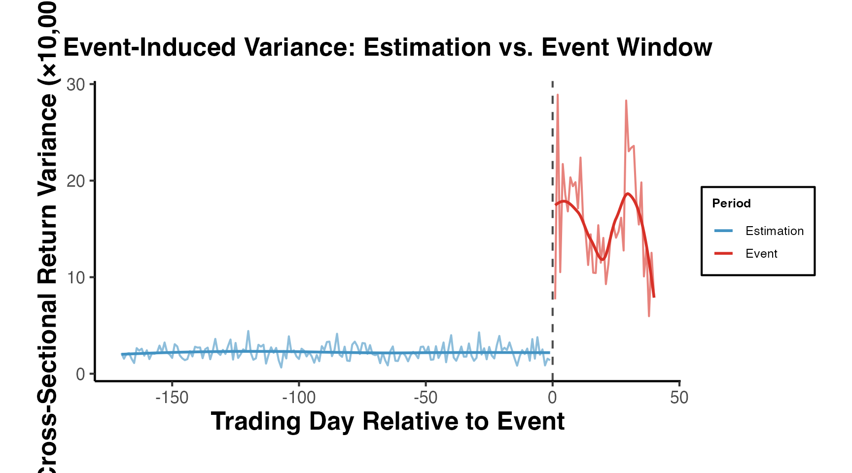
19.3 Announcement Returns vs. Pre-Announcement Drift
Detecting pre-announcement drift (returns accumulating before the official event date) is important for assessing information leakage and insider trading. A simple cumulation of pre-event abnormal returns tests for this.
set.seed(55)

# Simulate: pre-announcement drift for ~30% of observations (information leakage)
n_firms_d <- 40
leakage   <- rbinom(n_firms_d, 1, 0.3)  # 30% have leakage

# Full CAR time series: days -20 to +5
days_range <- -20:5
car_matrix <- matrix(0, nrow = n_firms_d, ncol = length(days_range))

for (i in seq_len(n_firms_d)) {
    true_drift <- if (leakage[i] == 1) {
        # Drift: starts accumulating 10 days before event
        c(rep(0, 10), cumsum(rnorm(10, 0.003, 0.005)),
          rnorm(6, 0.001, 0.010))
    } else {
        cumsum(rnorm(length(days_range), 0, 0.008))
    }
    car_matrix[i, ] <- true_drift
}

# Average across firms
caar_drift <- data.frame(
    day  = days_range,
    caar = colMeans(car_matrix),
    se   = apply(car_matrix, 2, sd) / sqrt(n_firms_d)
)
caar_drift$ci_lo <- caar_drift$caar - 1.96 * caar_drift$se
caar_drift$ci_hi <- caar_drift$caar + 1.96 * caar_drift$se

ggplot(caar_drift, aes(x = day, y = caar * 100)) +
    geom_ribbon(aes(ymin = ci_lo * 100, ymax = ci_hi * 100),
                fill = "#4393C3", alpha = 0.25) +
    geom_line(color = "#2166AC", linewidth = 1.2) +
    geom_vline(xintercept = 0, linetype = "dashed", color = "gray30") +
    geom_hline(yintercept = 0, color = "gray60") +
    annotate("text", x = -8, y = max(caar_drift$caar * 100) * 0.5,
             label = "Pre-announcement\ndrift", color = "firebrick",
             size = 3.5) +
    labs(
        title    = "CAAR with Pre-Announcement Drift Detection",
        subtitle = "Upward drift before day 0 may indicate information leakage",
        x        = "Trading Day Relative to Event",
        y        = "CAAR (%)"
    ) +
    causalverse::ama_theme()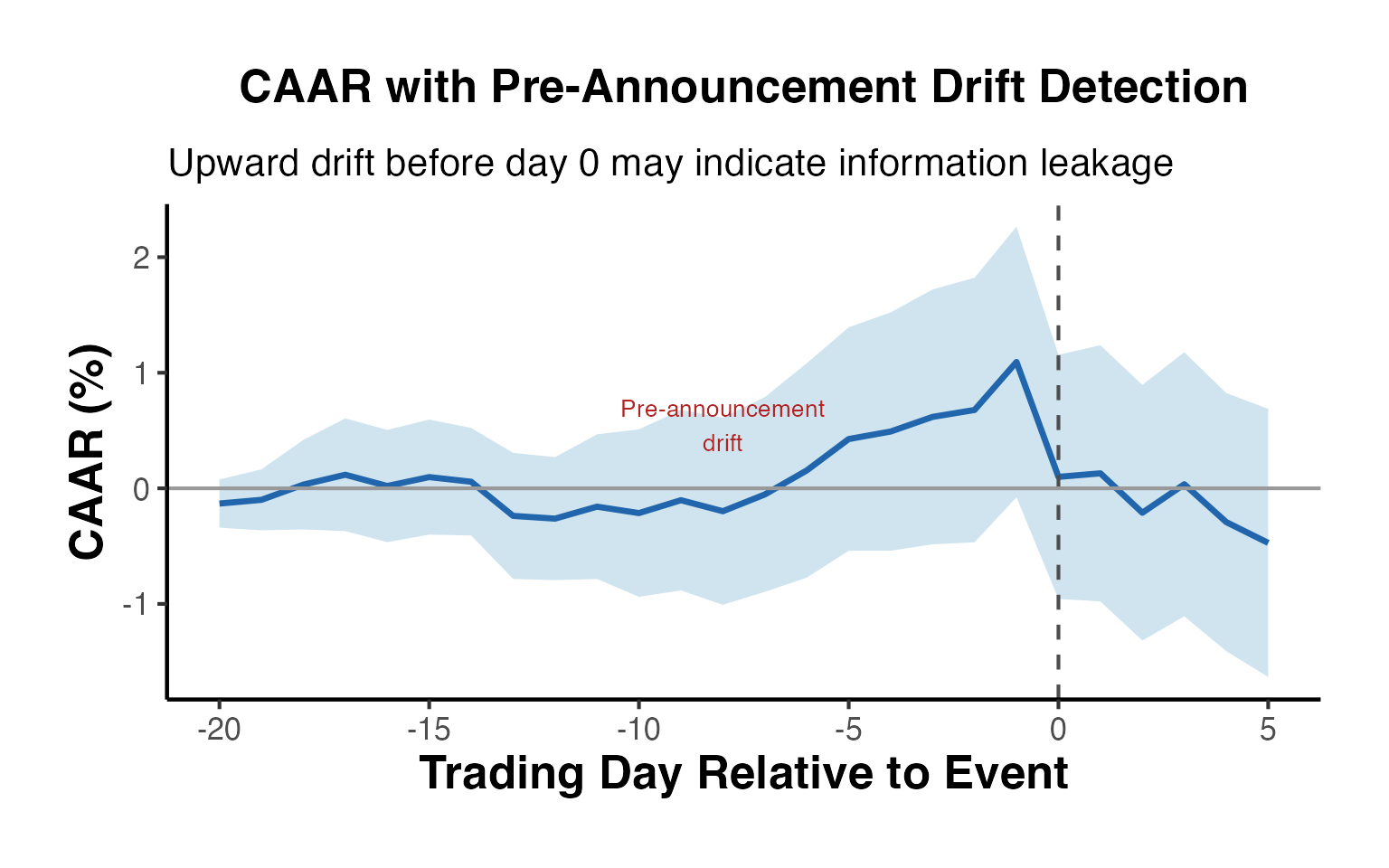
20. References
Ball, R., & Brown, P. (1968). An empirical evaluation of accounting income numbers. Journal of Accounting Research, 6(2), 159-178.
Bhagat, S., & Romano, R. (2002). Event studies and the law: Part II: Empirical studies of corporate law. American Law and Economics Review, 4(2), 380-423.
Boehmer, E., Musumeci, J., & Poulsen, A. B. (1991). Event-study methodology under conditions of event-induced variance. Journal of Financial Economics, 30(2), 253-272.
Brown, S. J., & Warner, J. B. (1980). Measuring security price performance. Journal of Financial Economics, 8(3), 205-258.
Brown, S. J., & Warner, J. B. (1985). Using daily stock returns: The case of event studies. Journal of Financial Economics, 14(1), 3-31.
Campbell, J. Y., Lo, A. W., & MacKinlay, A. C. (1997). The Econometrics of Financial Markets. Princeton University Press.
Carhart, M. M. (1997). On persistence in mutual fund performance. Journal of Finance, 52(1), 57-82.
Corrado, C. J. (1989). A nonparametric test for abnormal security-price performance in event studies. Journal of Financial Economics, 23(2), 385-395.
Dimson, E. (1979). Risk measurement when shares are subject to infrequent trading. Journal of Financial Economics, 7(2), 197-226.
Fama, E. F. (1998). Market efficiency, long-term returns, and behavioral finance. Journal of Financial Economics, 49(3), 283-306.
Fama, E. F., & French, K. R. (1993). Common risk factors in the returns on stocks and bonds. Journal of Financial Economics, 33(1), 3-56.
Fama, E. F., Fisher, L., Jensen, M. C., & Roll, R. (1969). The adjustment of stock prices to new information. International Economic Review, 10(1), 1-21.
Kolari, J. W., & Pynnonen, S. (2010). Event study testing with cross-sectional correlation of abnormal returns. Review of Financial Studies, 23(11), 3996-4025.
Kothari, S. P., & Warner, J. B. (2007). Econometrics of event studies. In B. E. Eckbo (Ed.), Handbook of Empirical Corporate Finance (Vol. 1, pp. 3-36). Elsevier.
MacKinlay, A. C. (1997). Event studies in economics and finance. Journal of Economic Literature, 35(1), 13-39.
Mitchell, M. L., & Stafford, E. (2000). Managerial decisions and long-term stock price performance. Journal of Business, 73(3), 287-329.
Patell, J. M. (1976). Corporate forecasts of earnings per share and stock price behavior: Empirical tests. Journal of Accounting Research, 14(2), 246-276.
Scholes, M., & Williams, J. (1977). Estimating betas from nonsynchronous data. Journal of Financial Economics, 5(3), 309-327.