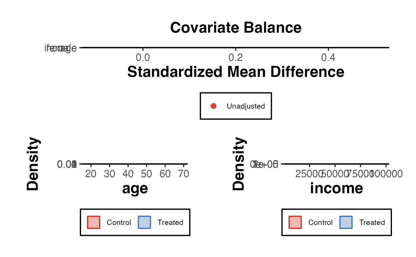
Comprehensive Balance Plot Suite — balance

Produces a multi-panel diagnostic figure comparing covariate distributions between treatment and control groups. Combines a standardized mean difference (SMD) dot plot, density overlays, and (optionally) a variance ratio panel. Useful for assessing balance before and after matching or weighting.

Usage

balance_plot(
  data,
  treatment,
  covariates = NULL,
  data_adj = NULL,
  weights = NULL,
  threshold = 0.1,
  var_labels = NULL,
  show_density = TRUE,
  show_variance_ratio = FALSE,
  title = "Covariate Balance"
)

Arguments

data: A data frame.
treatment: Character. Name of the binary treatment variable (0/1).
covariates: Character vector. Names of covariates to plot. Defaults to all numeric variables except treatment.
data_adj: A second data frame (e.g., post-matching) to overlay as "adjusted" estimates. Optional.
weights: Numeric vector. Case weights for the adjusted sample (alternative to data_adj). Length must equal nrow(data).
threshold: Numeric. SMD threshold line. Default 0.1.
var_labels: Named character vector. Display names for covariates.
show_density: Logical. Add density overlay panels. Default TRUE.
show_variance_ratio: Logical. Add variance ratio panel. Default FALSE.
title: Character. Overall plot title.

Value

A ggplot2 object (or patchwork figure if multiple panels).

Examples

set.seed(42)
n <- 300
df <- data.frame(
  treat  = rbinom(n, 1, 0.5),
  age    = rnorm(n, 40, 10),
  income = rnorm(n, 50000, 15000),
  female = rbinom(n, 1, 0.5)
)
# Introduce imbalance
df$age[df$treat == 1] <- df$age[df$treat == 1] + 5

balance_plot(df, treatment = "treat",
             covariates = c("age", "income", "female"))